Tina Memo No. 2002-005

Report sponsored by BAe Systems, Bristol.

Tutorial at BMVC, Manchester, 2001.

Tutorial at EUTIST IMV Pisa, 2001.

Tutorial at ECCV, Copenhagen, 2002.

Tutorial at Intelligent Vehicles Workshop, Paris, 2002.

Lectures at EPSRC Machine Vision Summer School, Surrey 2002-05, Kingston 2006, East Anglia 2007, Essex 2008.

Now including comments from prominent researchers in the field of computer and machine vision.

An Empirical Design Methodology for the Construction of

Machine Vision Systems.N.A.Thacker, A.J.Lacey, P.Courtney and G. S. Rees1

Last updated9/10/2005

Imaging Science and 1 Informatics Group,Biomedical Engineering Division, Advanced Information Processing Dept,

Medical School, University of Manchester, BAE Systems Ltd.,Stopford Building, Oxford Road, Advanced Technology Centre - Sowerby,

Manchester, M13 9PT. Filton, Bristol BS34 7QW.

Abstract

This document presents a design methodology the aim of which is to provide a framework forconstructing machine vision systems. Central to this approach is the use of empirical design techniquesand in particular quantitative statistics. The methodology described herein underpins the developmentof the TINA [26] open source image analysis environment which in turn provides practical instantiationsof the ideas presented.

The appendices form the larger part of this document, providing mathematical explanations of thetechniques which are regarded as of importance. A summary of these appendices is given below;

Appendix Title

A Maximum LikelihoodB Common Likelihood FormulationsC Covariance EstimationD Error PropagationE Transforms to Equal VarianceF Correlation and IndependenceG Modal ArithmeticH Monte-Carlo TechniquesI Hypothesis TestingJ Honest ProbabilitiesK Data FusionL Receiver Operator Curves

Comments on this document from prominent computer vision researchers and our responses to them are alsoprovided so that this work can be set in the context of current attitudes in the field of computer vision.

Acknowledgements

The authors would like to acknowledge the support of the EU PCCV (Performance Characterisation of ComputerVision Techniques) IST-1999-14159 grant. The authors are also grateful to the numerous people who have reviewedand commented on both this paper and the ideas behind it. These include Adrian Clarke, Paul Whelan, JohnBarron, Emanuel Truecco and Mike Brady. Finally the authors would like to acknowledge Ross Beveridge, KevinBowyer, Henrik Christensen, Wolfgang Foerstner, Robert Haralick and Jonathan Phillips for their contributionsto the area and whose work has inspired this paper.

An Empirical Design Methodology for the Construction of

Machine Vision Systems

N. A. Thacker, A. J. Lacey, P. Courtney 1G. ReesImaging Science and 1 Infomatics Group,

Biomedical Engineering Division, Advanced Information Processing Dept,Medical School, University of Manchester, BAE Systems Ltd.,

Stopford Building, Oxford Road, Advanced Technology Centre - Sowerby,Manchester, M13 9PT. Filton, Bristol BS34 7QW.

email: [neil.thacker],[a.lacey]@man.ac.uk

1 Background

Our approach to the construction and evaluation of systems is based upon what could be regarded as a set of selfevident propositions.

• Vision algorithms must deliver information allowing practical decisions regarding interpretation of an image.

• Probability is the only self-consistent computational framework for data analysis, and so must form the basisof all algorithmic analysis processes.

• The most effective and robust algorithms will be those that match most closely the statistical properties ofthe data.

• A statistically based algorithm which takes correct account of all available data will yield an optimal result1.

Attempting to solve vision problems of any real complexity necessitates, as in other engineering disciplines, amodular approach (a viewpoint popularised as a model for the human vision system by David Marr [16]). Thereforemost algorithms published in the machine vision literature attend to only one small part of the “vision” problem,with the implicit intention that the algorithm could form part of a larger system2. What follows from this is thatbringing these together as components in a system requires that the statistical characteristics of the data generatedby one module match the assumptions underpinning the next.

In many practical situations problems cannot be easily formulated to correspond exactly to a particular compu-tation. Compromises have to be made, generally in assumptions regarding the statistical form of the data to beprocessed, and it is the adequacy of these compromises which will ultimately determine the success or failure ofa particular algorithm. Thus, understanding the assumptions and compromises of a particular algorithm is anessential part of the development process. The best algorithms not only model the underlying statistics of themeasurement process but also propagate these effects through to the output. Only if this process is performedcorrectly will algorithms form robust components in vision systems.

The evaluation of vision systems cannot be separated from the design process. Indeed it is important that the systemis designed for test by adopting a methodology within which performance criteria can adequately be defined. Whena modular strategy is adopted, system testing can be usefully considered as a two stage process [19] (summarisedin figure 1);

• the evaluation of the statistical distributions of the data and comparison with algorithmic assumptions inindividual modules; technology evaluation,

• the evaluation of the suitability of the entire system for the solution of a particular type of task; scenario

evaluation.

The process of scenario evaluation is often time consuming and not reusable. The process of technology evaluationis complex and involves multiple objectives, however the results are reusable for a range of applications. It therefore

1Where the definition of optimal can be unambiguously defined by the statistical specification of the problem.2Though it could be argued that many researchers have lost focus on the bigger problem and thus the true motivations of a modular

approach.

3

distributions assumptions. distributions assumptions. distributions

data datadata module module

algorithm 1 algorithm 2

scenario evaluation

technology evaluation

outputinput

Figure 1: Scenario and Technology evaluation in a two stage statistical data analysis system.

merits effort and should be attempted. Ideally, we would like to be able to specify a limited set of summary variableswhich define the requirements of the input data and the main characteristics of the output data, in a manner similarto an electronic component databook [25]. However, it must be remembered that it is the suitability of the outputdata for use in later modules which defines performance, and in some circumstances it may not be easy (or evenpossible) to define performance independent of practical use of the data. For instance, problems can arise whenthe output data of one algorithm is to be fed into several subsequent algorithms, each having different or evenconflicting requirements. The most extreme example of this is perhaps scene segmentation where, in the absenceof a definite goal, a concise method for the evaluation of such algorithms is likely to continue to be a challenge [22].

Machine vision research has not emphasised the need for (or necessary methods of) algorithm characterisation.This is rather unfortunate, as the subject cannot advance without a sound empirical base [11]. In our opinion thisproblem can generally be attributed to one of two main factors; a poor understanding of the role of assumptionsand statistics; and a lack of appreciation of what is to be done with the generated data. The assumptions behindmany algorithms are rarely clearly stated and it is often left to the reader to infer them3. The failure to presentclearly the assumptions of an algorithm often leaves the reader confused as to the novel or valid aspects of thepublished research and can give the impression that it is possible to create good algorithms by accident ratherthan design. In addition, the inability to match algorithms to tasks may lead those who require practical solutionsto real problems to conclude that little (if anything) published in this area really works. When in fact, virtuallyall published algorithms can be expected to work, provided that the input data satisfy the assumptions implicit inthe technique. It is the unrealistic nature of these assumptions (e.g. noise free data) which is more likely to renderalgorithms useless.

The following is a description of a methodology for the design of vision module components. This methodologyfocuses on identifying the statistical characteristics of the data and matching these to the assumptions of particulartechniques. The methods given in the appendices have been drawn from over a decade of vision system designand testing, which has culminated in the construction of the TINA machine vision system [26]. These includea combination of standard techniques and less standard ones which we have been developed to address specificproblems in algorithm design.

2 Technology and Scenario Evaluation

There are several common models for statistical data analysis, all of which can be related at some stage tothe principle of maximum likelihood (appendix A). This framework provides methods for the estimation andpropagation of errors, which are essential for characterising data at all stages in a system. Likelihood basedapproaches begin by assuming that the data under analysis conforms to a particular distribution. This distributionis used to define the probability of the data given an assumed model (appendix B).

3A process we have previously called “inverse statistical identification” an allusion to the analogous problem of system identificationin control theory.

4

Example Task Data Error Assumption

Basic Data Images Uniform random GaussianStatistical Analysis Histograms Poisson sampling statisticsShape Analysis Edge location Gaussian perpendicular to edge

Line fits Uniform Gaussian on end-pointsMotion Corner features Circular (Elliptical) Gaussian3D Objection Location Stereo data Uniform in disparity space

Table 1: Standard error model assumptions.

2.1 Input data

The first step in evaluating an algorithmic module is identification of the appropriate model and empirical con-firmation of the distribution with sample data. Appropriate methods for this task include; correlation analysis,histogram fitting and the Kolmogorov-Smirnov test [24]. The interpretation of the results from such processes re-quire knowledge of the consequences of deviation from the expected distribution. In general, the greatest problemsare caused by outliers (see below) although, the closer the data distributions conform to the assumed model, thebetter the expected results. Assumptions which prove valid for one algorithm, can often prove useful in the designof new algorithms. Some distributions commonly used in the machine vision literature are listed in table 1.

Although there are no general restrictions on the shape of these distributions the most common are Gaussian,Binomial, Multinomial and Poisson. These correspond to commonly occurring data generation processes. Thecentral limit process ensures that the assumption of Gaussian distributed data forms the basis of many algorithms.This leads to tractable algorithms as the log-likelihood formulation of a Gaussian assumed model often takesthe particularly simple form of a least-squares statistic, which can often be formulated as a closed form solution(appendix B). It is therefore useful to know that certain non-linear functions will transform the other commondistributions to a form which approximates a Gaussian with sufficient accuracy to enable least-squares solutionsto be employed.

Unfortunately, most practical situations generate data with long tailed distributions (outliers). The problemsassociated with outliers in data analysis are well known. However, what appears less well understood is thereason for the complete lack of closed form solutions based upon a long tailed distribution. By definition only asimple quadratic form (or monotonic mapping thereof) for the log-likelihood, can be guaranteed to have a uniqueminimum. Long tailed (non-Gaussian) likelihood distributions inevitably result in multiple local minima whichcan only be located by explicit search (e.g. the Hough transform) or optimisation (e.g. gradient descent).

Other assumptions in the likelihood formulation generally include those of data independence. Independence canbe confirmed by plotting joint distributions. Uncorrelated data will produce joint distributions which are entirelypredicted by the outer product of the marginal distributions (appendix F). Correlations (the lack of independence)in data can have several consequences. Strong correlations may produce suboptimal estimates from the algorithmand covariances may not concisely describe the error distribution.

2.2 Output data

The next step in module analysis is to estimate the errors on the output data. If the output is the result of a log-likelihood measure then errors can be computed using covariance estimation (appendix C). Covariance estimationis possible even in the presence of outliers, provided that a robust kernel is used [17]. If the output quantitiesfrom a module are computed from noisy data the errors on the results can be calculated using error propagation(appendix D). Both of these theoretical techniques assume Gaussian distributed errors and locally linear behaviourof the algorithmic function.

These assumptions require validation (i.e. checks to ensure that the theory is an accurate representation of reality),which can be achieved using Monte-Carlo approaches (appendix H). Once again, techniques such as histogramming,fitting and Kolmogorov-Smirnov tests are useful. High degrees of non-linear behaviour can be addressed using atechnique we call modal arithmetic [30] (appendix G). Non-linear transformation of estimated variables may benecessary in order to make better approximations to Gaussian distributions. It may also be necessary to combinevariables in order to eliminate data correlation. The definition of the parameters passed between algorithmscan be substantially different to naive expectation e.g. 3D data from a stereo algorithm is best represented indisparity space (appendix E). Selecting data representations which provide appropriate descriptions of statistical

5

distributions is of fundamental importance 4. Notice, the evaluation process has a direct influence on the processof system design, under-scoring the earlier statements that system design and performance evaluation cannot (andshould not) be treated separately.

In many cases the division of tasks into modules will be driven by the statistical characteristics of the processed dataand cannot be specified a priori without a very clear understanding of the expected characteristics of all systemmodules. Given the source of data typical of machine vision applications it is also very likely that algorithms willproduce outlier data which cannot be eliminated by transformation or algorithmic improvement and will thereforerequire appropriate (robust) statistical treatment in later modules (see appendix L).

A rigid application of the above design and test process (see figure 2) will produce verifiable optimal outputs fromeach module. Ultimately however, we will need to know if this data is of sufficient quality to achieve a particulartask, a process we will call scenario evaluation. Under many circumstances it should be sufficient to determinethe required accuracy of the output data in order to achieve this task. Alternatively, the covariance estimates fromthe technology evaluation could be used to quantify the expected performance of the system on a per-case basis.

Statistical measures of performance can be obtained by testing on a representative set of data. We would anticipatethe need to compute the probability of a particular hypothesis, either as a direct interpretation of scene contentsor as the likely outcome of an action (appendix I). Such probabilities are directly testable by virtue of beinghonest probabilities (appendix J). The term honest simply means the computed probability values should directlyreflect the relative frequency of occurrence of the hypothesis in sample data (classification probabilities P (C|data)should be wrong 1 − P (C|data) of the time). Tested hypotheses, such as a particular set of data being generatedby a particular model, should have a uniform probability distribution. Direct confirmation of such characteristicsprovide powerful tools for the quantitative validation of systems and provide mechanisms for self test during use.

Often, we will need to construct systems which are not simply a series of sequential operations. It is quite likelythat vision modules might provide evidence from several independent sources. Under these conditions we will needto perform a data fusion operation. Within the probabilistic framework described above there are three ways ofachieving this; combination of probability (using a learning technique such as a neural network), combination oflikelihoods (using covariances), and combination of hypothesis tests. All three of these are described in greaterdetail in appendix K.

3 Identifying Candidate Modules from the Literature

Armed with the above methodology we are in a position to evaluate work in the machine vision literature in termsof its likely suitability for use in a vision system. In fact we can generate a short list of questions which exemplifythose we should attempt to answer when evaluating a module for inclusion in a system.

• Does the paper make clear the task of the module?

• Are the assumptions used in algorithm design stated?

• Is the work based upon (or related to) a quantitative statistical framework?

• Are the assumed data distributions realistic i.e. representative of the data available in the considered situa-tion?

• Has the computation of covariances been derived and tested?

• Does the theoretical prediction of performance match practical reality?

• Is the output data in a suitable form for use in any subsequent system?

The poor intersection between this list and general academic interests in this area (such as novelty and mathematicalsophistication) underscores the main problems faced by those attempting to construct practical systems.

Notice that this list does not include system testing on typical image datasets, as that would be regarded asscenario rather than technology evaluation. Scenario evaluation, without considering the statistical characteristicsof the data, is likely to be of much less value in the development of re-usable modules as the results will be taskspecific. Unfortunately, when performance characterisation is carried out in the literature it is very often a scenarioevaluation. This goes against the implied assumption that most vision research is ultimately intended for use in alarger system.

4yet is often overridden by preconceived ideas of algorithm design.

6

Test DataAvailable?

Failure

StandardDistribution?

Yes

No

Transformation

Yes

No

Approx.Gaussian?

Yes

DirectComputation?

Yes

StatisticalStability?

Yes

Independence?No

DecorrelationNo

Log−Likelihood

Outliers?

Robust Statistics

Covariance Estimation

IterativeLeast Squares

Error Propagation

Yes

Yes

ValidCovariances?

Closed FormSolution?

No

Yes

Modal Arithmetic

Yes

Equal Variance Transform

No

No

No

No

Success

Yes

Subsequent module path

BootstrapTechniques

Figure 2: Technology evaluation flow chart. This diagram identifies the major design decisions which must beaddressed in order to deliver quantified outputs from an algorithm. Transforms are suggested at various stagesin order to solve problems associated with non-Gaussian behaviour. The label Bootstrap is intended to refer tocustom made statistical measures constructed from sample data.

4 Summary and Conclusions

This document suggests a quantitative statistical approach to the design and testing of machine vision systemswhich could be considered as an extension of methodologies suggested by other authors [3, 12]. We have focused

7

on the use of likelihood and hypothesis testing paradigms and it would be natural for a reader familiar with themachine vision literature to feel that we have missed out other approaches which have (or have had) a higherprofile in the literature (e.g. computational geometry and image analysis as inverse optics). However, we wouldargue that for the modular approach to system building to succeed we must have appropriate control over thestatistical distributions generated during analysis. This is possible with likelihood based techniques because theyenable the construction of measures to determine the best interpretation of the data (such as least squares) andalso allow quantitative predictions to be made of the stability of estimated parameters (such as covariances). Themachine vision problem, therefore, does not stop once a closed form solution is found (see [13] for a discussion ofthe use of statistics in closed form solutions). Inevitably, to acquire quantitative data for use in a system, erroranalysis will be required. This difficult step is often missing in the work found in the literature, yet attempting todo it can completely alter our understanding of the apparent value or even validity of the approach. The work ofMaybank [15] demonstrated exactly this point with regard to the use of affine invariants for object recognition.

The reader may at this point feel that there is a broader context for probability theory than likelihoods andhypothesis testing. In particular likelihood based techniques have well known limitations, such as bias in finitesamples [8]. The problem of model selection [28] is endemic in the machine vision area and likelihoods cannotbe directly compared between two different model hypotheses. Approaches which aim to directly address theseissues are thus acceptable extensions to the above methodology. However, some popular areas of probability theorydo not (at least yet) have comparable quantitative capabilities (e.g. Bayesian approaches) and may therefore beunsuitable for system building. We have made an attempt to summarise these issues in [5]. It remains to be seenwhether advocates of these approaches and others (such as Dempster-Schafer theory) are able to address theseissues.

Other approaches to algorithm design use methods which are based upon apparently different principles, such asentropy and mutual information [31]. However, we regard these as only alternative ways to formulate problems andbelieve that most experienced researchers would accept that all approaches should be reconcilable with probabilitytheory. Thus if there already exists a likelihood based formulation of the technique, this should be taken asthe preferred approach. Obviously, if the research community as a whole accepted this viewpoint many paperswould already have been written and presented differently. As the construction of systems from likelihood basedformulations is generally likely to require optimisation of robust statistics, generic algorithms for the location ofmultiple local optima should be regarded as a fundamental research issue. So too should the problem of covarianceestimation from common optimisation tasks and popular algorithmic constructs, (such as Hough transforms), whichhave already been shown to be consistent with likelihood approaches [23, 1].

Many attempts at algorithmic evaluation in the literature focus on the specification of particular performancemetrics. Although these metrics may give some indication as to the basic workings of an algorithm, quantitativeevaluation should set as the ultimate goal an understanding of the performance of the system. Performance metricsfor modules should therefore be specified with this in mind.

Non-quantitative evaluation is probably of more use in the early stages of algorithm construction than duringthe final integration into a system. However, in the methodology described a key aspect is the identificationof assumptions. Knowledge of these assumptions (and suitable methods for determining their validity) allowscomparisons of algorithms to be carried out at the theoretical level. Also, we should not be surprised whenalgorithms which are built upon the same set of founding assumptions within a sensible probabilistic framework,give near identical performance. This has been well illustrated in several pieces of work including that by Fisheret al. [10], where alternative techniques for location of 3D models in 3D range data were found to give equivalentresults to within floating point accuracy. If careful statistical analysis of data did not give this result then itwould be an indication that probability theory itself was not self-consistent. Also, when performing comparativetesting of modules we should be aware that algorithmic scope, as determined by the restrictions imposed by theassumptions, should be taken into account in the final interpretation of results. Algorithms which give apparentlyweaker performance on the basis of performance metrics may still be more applicable for some tasks. A simpleexample of this is that least squares fitting will generally give a better bounded estimate of a set of parametersthan robust techniques, yet robust techniques are essential in the presence of outliers. An evaluation of thesetwo techniques in the absence of outliers would incorrectly conclude that least-squares was always more accurate.Clearly this result is of limited use when building practical systems.

8

A Maximum Likelihood

A more detailed treatment of the theory and techniques of Maximum Likelihood statistics can be found in [8]. Asummary of the theory is presented here for completeness.

For n events with probabilities computed assuming a particular interpretation of the data Y (for example a model)

P (X0X1X2...Xn|Y )P (Y ) = P (X0|X1X2...XnY )P (X1|X2...XnY )......P (Xn|Y )P (Y )

Maximum Likelihood statistics involves the identification of the event Y which maximises such a probability. Inthe absence of any other information the prior probability P (Y ) is assumed to be constant for all Y . For largenumbers of variables this is an impractical method for probability estimation. Even if the events were simple binaryvariables there are clearly an exponential number of possible values for even the first term in P (XY ) requiringa prohibitive amount of data storage. In the case where each observed event is independent of all others we canwrite

P (X |Y ) = P (X0|Y )P (X1|Y )P (X2|Y )...P (Xn|Y )

This is a more practical definition of joint probability but the requirement of independence is quite a severerestriction. However, in some cases data can be analysed to remove these correlations, in particular the use ofan appropriate data model (such as in least squares fitting) and processes for data orthogonalisation (includingprinciple component analysis). For these reasons all common forms of maximum likelihood definitions assume dataindependence.

Probability independence is such an important concept it is worth defining carefully. If knowledge of the probabilityof one variable A allows us to gain knowledge about another event B then these variables are not independent.Put in a way which is easily visualised, if the distribution of P (B|A) over all possible values of B is constant forall A then the two variables are independent. Assumptions of independence of data can be tested graphically byplotting P (A) against P (B) or A against B if the variables are directly monotonically related to their respectiveprobabilities.

On a final point. We have derived maximum-likelihood here as a subset of Bayes theory. This may lead to thenatural assumption that re-inclusion of the prior probabilities (as a function of parameter value) is an appropriatething to do. However, one of the advantages of the likelihood formulation is that the optimum interpretation isinvariant to the choice of equivalent parameterisation of the problem (though not invariant to choice of measurementsystem see appendix E). For example we can represent a rotation matrix as a quaternion or as rotation angles,the optimum representation (and therefore the equivalent rotation matrix) will always be defined at an equivalent(statistical) location. If however we re-introduce the Bayes priors we have the problem of specifying a distribution,and this is equivalent to saying that there is a natural representation for the model. From a quantitative perspectivesuch an approach can only be justified in circumstances where there is a deterministic generator of the model (suchas a fixed physical system). Following this line of reasoning one can come to the conclusion that although Bayestheory is suitable for determining the probability associated with an optimal interpretation of the data it shouldnot be used for quantification unless the penalties of bias are fully understood and accounted for. Maximumlikelihood is the only way of getting an (largely) un-biased estimate of the parameters. It is reasonable to assessthe interpretation of a model choice on the basis of a set of parameters determined using the likelihood, it isgenerally not reasonable to directly bias the parameter estimates using the prior probabilities if they are requiredfor a quantitative purpose.

9

B Common Likelihood Formulations

Dealing with Binary Evidence

The simplest likelihood model is for binary observations of a set of variables with known probabilities. If wemake the assumption that the event Xi is binary with probability P (Xi) then we can construct the probability ofobserving a particular binary vector X as:

P (X) = Πi(P (Xi)Xi (1 − P (Xi))

(1−Xi)

The log likelihood function is therefore

log(P ) =∑

i

Xilog(P (Xi)) + (1 − Xi)log(1 − P (Xi))

This quantity can be minimised or directly evaluated in order to form a statistical decision regarding the likelygenerator of X . This is therefore a useful equation for methods of statistical pattern recognition.

If we now average many binary measures of X into the vector O we can compute the mean probability of observingthe distribution O generated from P (X) as;

< log(P ) >=∑

i

O(Xi)logP (Xi) + (1 − O(Xi))log((1 − P (Xi))

It should be noted that this is not the log probability that O is the same distribution as P as it is asymmetricunder interchange of O and P. To form this probability we would also have to test for P being drawn from thedistribution O. The resulting form of this comparison metric is often referred to as the log entropy measure as themathematical form (and statistical derivation) is analogous to some parts of statistical mechanics in physics.

Poisson and Gaussian Data Distributions

A very common problem in machine vision is that of determining a set of parameters in a model. Take for examplea set of data described by the function f(a, Yi) where a defines the set of free parameters defining f and Yi is thegenerating data set. If we now define the variation of the observed measurements Xi about the generating functionwith some random error we can see that the probability P (X0|X1X2...XNaY0) will be equivalent to P (X0|aY0) asthe model and generation point completely define all but the random error.

Choosing Gaussian random errors with a standard deviation of σi gives;

P (Xi) = Aiexp(−(Xi − f(a, Yi))

2

2σ2i

)

where Ai is a normalisation constant. We can now construct the maximum likelihood function;

P (X) = ΠiAiexp(−(Xi − f(a, Yi))

2

2σ2i

)

which leads to the χ2 definition of log likelihood;

log(P ) =−1

2

∑

i

(Xi − f(a, Yi))2

σ2i

+ const

This expression can be maximised as a function of the parameters a and this process is generally called a leastsquares fit. Whenever least squares is encountered there is an implicit assumption of independence and of aGaussian distribution. In practical situations the validity of these assumptions should be checked by plotting thedistribution of Xi − f(a, Yi) to make sure that it is Gaussian.

Often when working with measured data we need to interpret frequency distributions of continuous variables, forexample in the form of frequency histograms. In order to do this we must know the statistical behaviour of these

10

measured quantities. The generation process for a histogram bin quantity (making an entry at random accordingto a fixed probability) is strictly a multi- distribution, however for large numbers of data bins this rapidly becomeswell described by the Poisson distribution. The probability of observing a particular number of hi for an expectedprobability of pi is given by;

P (hi) = exp(−pi)pk

i

hi!

For large expected numbers of entries this distribution approximates a Gaussian with σ =√

hi. The limit ofa frequency distribution for an infinite number of samples and bins of infinitesimal width defines a probabilitydensity distribution. These two facts allow us to see that the standard χ2 statistic is appropriate for comparingtwo frequency distributions hi and ji for equal sized samples;

χ2 =∑

i

(hi − ji)2/(hi + ji)

This equation has the restriction that it is not defined in the region where hi + ji = 0. We can overcome thisproblem by transforming the data to a domain where the errors are uniform by taking square roots. This processnot only reduces the Gaussian approximation error but also removes the denominator. The common form of thisis the probability comparison metric known as the Matusita distance measure LM ;

LM =∑

i

(√

P1(Xi) −√

P2(Xi))2

This can be rewritten in a second form;

= 2 − 2∑

i

√

(P1(Xi)P2(Xi))

Where the second term defines the Bhattacharyya distance metric LB;

LB =∑

i

√

P1(Xi)√

P2(Xi)

For discrete signals [28];

χ2 = 4 − 4∑

i

√

hiji

11

C Covariance Estimation

The concept of error covariance is very important in statistics as it allows us to model linear correlations betweenparameters. For locally linear fit functions f we can approximate the variation in a χ2 metric about the minimumvalue as a quadratic. We will examine the two dimensional case first where the quadratic formula is;

z = a + bx + cy + dxy + ex2 + fy2

This can be re-written in matrix algebra as;

χ2 = χ20 + ∆XT C−1

x ∆X

where C−1x is defined as the inverse covariance matrix thus;

C−1x =

u vw s

Comparing this with the original quadratic equation gives;

χ2 = χ20 + ∆X2u + ∆Y ∆Xw + ∆X∆Y v + ∆Y 2s

where;

a = χ20, b = 0, c = 0, d = w + v, e = u, f = s

Notice that the b and c coefficients are zero as required if the χ2 is at the minimum. In the general case we needa method for determining the covariance matrix for model fits with an arbitrary number of parameters. Startingfrom the χ2 definition using the same notation as previously;

χ2 =1

2

N∑

i

(Xi − f(Yi, a))2

σ2i

We can compute the first and second order derivatives as follows;

∂χ2

∂an

=

N∑

i

(Xi − f(Yi, a))

σ2i

∂f

∂an

∂2χ2

∂an∂am

=N

∑

i

1

σ2i

(∂f

∂an

∂f

∂am

− (Xi − f(yi, a))∂2f

∂an∂am

)

The second term in this equation is expected to be negligible compared to the first and with an expected value ofzero if the model is a good fit. Thus the cross derivatives can be approximated to a good accuracy by;

=

N∑

i

1

σ2i

(∂f

∂an

∂f

∂am

)

The following quantities are often defined;

βn =1

2

∂χ2

∂an

αnm =1

2

∂2χ2

∂an∂am

As these derivatives must correspond to the first coefficients in a polynomial (Taylor) expansion of the χ2;

C = α−1 where α =α11 α12 . . .α21 α22 . . .. . . . . . αnm

And the expected change in χ2 for a small change in model parameters can be written as;

∆χ2 = ∆aT α∆a

12

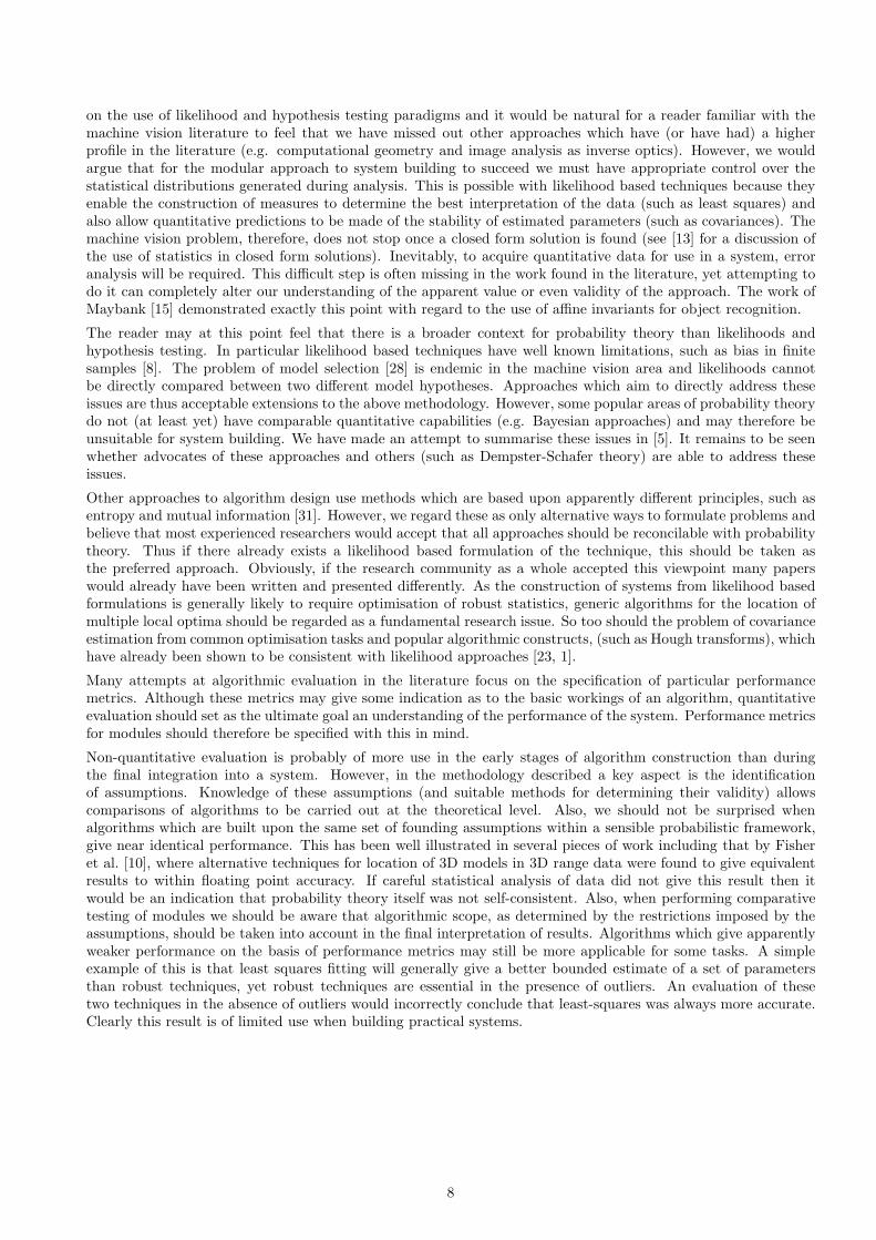
Process Calculation Theoretical ErrorAddition O = I1 + I2 ∆O2 = σ2

1 + σ22

Division O = I1I2

∆O2 =σ21

I22

+I21σ2

2

I42

Multiplication O = I1 . I2 ∆O2 = I22σ2

1 + I21σ2

2

Square-root O =√

(I1) ∆O2 =σ21

I1

Logarithm O = log(I1) ∆O2 =σ21

I21

Polynomial Term O = In1 ∆O2 = (nIn−1

1 )2σ21

Table 2: Error Propagation in Image Processing Operations

D Error Propagation

In order to use a piece of information f(X) derived from a set of measures X we must have information regardingits likely variation. If X has been obtained using a measurement system then we must be able to quantify theprecision of this system. Therefore, we require a method for propagating likely errors on measurements throughto f(X). Assuming knowledge of error covariance this can be done as follows;

∆f(X) = ∇fT CX∇f

The method simply uses the derivative of the function f as a linear approximation to that function. This issufficient provided that the expected variation in parameters ∆X is small compared to the range of linearity ofthe function. Application of this technique to even simple image processing functions gives useful informationregarding the expected stability of each method (Table 2) [7].

When the problem does not permit algebraic manipulation in this form (due to significant non-linear behaviourin the range of ∆f(X) or functional discontinuities) then numerical (Monte-Carlo) approaches may be helpful inobtaining the required estimates of precision (appendix H).

13

E Transforms to Equal Variance

The choice of a least squares error metric gives many advantages in terms of computational simplicity and isalso used extensively for definitions of error covariance and optimal combination of data (Appendices C and K). However, the distribution of random variation on the observed data X is something that generally we have noinitial control over and could well be arbitrary and so we have the problem of adjusting the measurements in orderto account for this. In addition, we have the problem that different choices for the way we represent the data willproduce different likelihood measures. Take for example a set of measurements made from a circle, we can chooseto measure the size of a circle as a radius or as an area. However, it can be easily shown that constructing alikelihood technique based upon sampled distributions will produce different (inconsistent) formulations for thesetwo representations of the same underlying data. Transferring the likelihood from a distribution of radial errorswill not produce the empirically observed distribution for area due the non-linear transformation between thesevariables. Which should we choose as correct (or are both wrong)? Initially these may be seen as separate problems,but in fact they are related and may have one common solution. To understand this we need to consider non-lineardata transformations and the reasons for applying them.

In many circumstances it is possible to make distributions more suitable for use of standard ML formulations (eg:least squares) by transformation g(Xi) and g(f(a, Yi)), where g is chosen so that the initial distribution of Xi mapsto an equal variance distribution (near Gaussian) in g. Examples of this for statistical distributions are the useof the square-root transform for Poisson distributed variables (appendix B) and the asin mapping for binomialdistributed data []. However, this problem can occur more generally due to the need to have to work with quantitieswhich are not measured directly.

One good example of this is in the location of a known object in 3D data derived from a stereo vision system.In the coordinate system where the viewing direction corresponds to the z axis, x and y measures have errorsdetermined by image plane measurement. However, the depth zi for a given point is given by;

zi = fI/(Xli − Xri)

where I is the interocular separation, f is the focal length and Xli and Xri are image plane measurements. Attemptsto perform a least squares fit directly in (x, y, z) space results in instability due to the non-Gaussian nature ofthe zi distribution. However, transformation to (x, y, 1/

√2z) yields Gaussian distributions and good results. In

general, observation of a dependency of the error distribution of a derived variable with that variable (in the abovecase the dependency of σz on z), is very often a sign that the likelihood distribution is skewed.

Any functional dependency of the errors on a measurement is a potential source of problem for subsequent algo-rithms. Building error estimates into the model is one possible way of attempting to solve this. This is the reasonthat in the standard statistical chi-squared test for comparing observed frequencies to a model estimates it is rec-ommended to estimate the data variance terms from theory rather than the data. In the context of an optimisationtask this is imperfect as such a process can introduce instabilities, bias and computational complexity. Ultimately,if the errors var(Xi) have function dependences h(f(a, Yi)) then we never really know the correct distribution for agiven measurement. The only way to avoid this is to work with data which have variances which are independentof the data value (i.e.: equal variances). For a known functional dependency h the transformation g which mapsthe variable Xi to one with equal variance follows directly from the method of error propagation and is given by;

g =

∫

1

h(X)dX

All of the transformations mentioned above can be generated from this process, including those which map standardstatistical distributions to more Gaussian ones, though the extent to which this is a general property of this methodis unclear. Ultimately the results of such transforms will need to be assessed on a case by case basis.

We are now also in a position to answer our questions regarding data representation in ML. The selection ofmeasured variables from the equal variance domain provides a unique solution to the problem of identification ofthe source data space. Such ideas deal directly with the key problem of applying probability (which is strictly onlydefined for binary events) to continuous variables by defining an effective quantisation of the problem accordingto measurable difference. In addition to the numerical issues involved it may also be reasonable to conclude thatthis is the only valid way of applying probability theory to continuous distributions. If this is true then it must besaid that it represents a considerable theoretical departure from commonly accepted use of these methods.

14

F Correlation and Independence

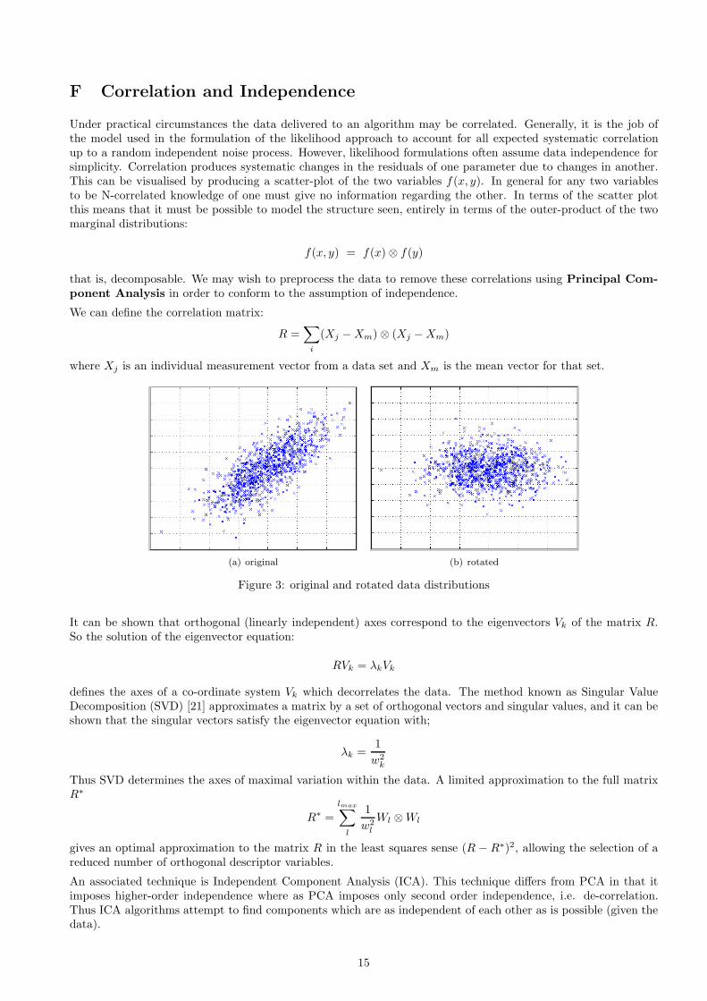
Under practical circumstances the data delivered to an algorithm may be correlated. Generally, it is the job ofthe model used in the formulation of the likelihood approach to account for all expected systematic correlationup to a random independent noise process. However, likelihood formulations often assume data independence forsimplicity. Correlation produces systematic changes in the residuals of one parameter due to changes in another.This can be visualised by producing a scatter-plot of the two variables f(x, y). In general for any two variablesto be N-correlated knowledge of one must give no information regarding the other. In terms of the scatter plotthis means that it must be possible to model the structure seen, entirely in terms of the outer-product of the twomarginal distributions:

f(x, y) = f(x) ⊗ f(y)

that is, decomposable. We may wish to preprocess the data to remove these correlations using Principal Com-

ponent Analysis in order to conform to the assumption of independence.

We can define the correlation matrix:

R =∑

i

(Xj − Xm) ⊗ (Xj − Xm)

where Xj is an individual measurement vector from a data set and Xm is the mean vector for that set.

(a) original (b) rotated

Figure 3: original and rotated data distributions

It can be shown that orthogonal (linearly independent) axes correspond to the eigenvectors Vk of the matrix R.So the solution of the eigenvector equation:

RVk = λkVk

defines the axes of a co-ordinate system Vk which decorrelates the data. The method known as Singular ValueDecomposition (SVD) [21] approximates a matrix by a set of orthogonal vectors and singular values, and it can beshown that the singular vectors satisfy the eigenvector equation with;

λk =1

w2k

Thus SVD determines the axes of maximal variation within the data. A limited approximation to the full matrixR∗

R∗ =

lmax∑

l

1

w2l

Wl ⊗ Wl

gives an optimal approximation to the matrix R in the least squares sense (R − R∗)2, allowing the selection of areduced number of orthogonal descriptor variables.

An associated technique is Independent Component Analysis (ICA). This technique differs from PCA in that itimposes higher-order independence where as PCA imposes only second order independence, i.e. de-correlation.Thus ICA algorithms attempt to find components which are as independent of each other as is possible (given thedata).

15

G Modal Arithmetic

Sometimes the effects of non-linear calculations on data with a noise distribution affects not only the variance ofthe computed quantity but also the mean value. From a likelihood point of view we can define the ideal resultfrom a computation as the most frequent (or modal) value that would have resulted from data drawn from theexpected noise distribution. We can find such values directly, via the process of Monte-Carlo (appendix H), butwe can also predict these values analytically. We have termed the algorithm design technique which addressed thisissue modal arithmetic.

The general method of modal arithmetic for a measured value with distribution D(x) and a non-linear functionf(x) would be to find the solution xmax of

∂[D(x)

∂f(x)/∂x]/∂x = 0

with the modal solution of f(xmax). Modal arithmetic is unconditionally stable, as peaks in probability distri-butions cannot occur at infinity. It also has much similarity with some approaches in statistics which advocatethe use of the mode rather than the mean as the most robust indicator of a distributed variable. The simplestexample of this is for image division where small errors on the data produce instabilities in computations involvinglarge quantities of data. Error propagation shows that a small change in the input quantity ∆x will give an erroron the corresponding output of

∆y =∆x

x2

which is clearly unstable for values of x which are comparable to its error. This problem can be understoodbetter by considering the distribution of computed values from the range of those available for input. We start byassuming a Gaussian distribution for the denominator.

Px = A exp(−(x − x0)2/2σ2)∆x

Where x0 is the central value of x with a standard deviation of σ. If we take a small area of data from theprobability distribution for x (i.e. Px = D(x)∆x), we can associate this with an equal number of solutions in theoutput space y (i.e. Py = D(y)∆y) (figure 4 (i) and (ii)) giving:

D(y) = A x2exp(−(x − x0)2/2σ2)

��������

��������

������������

������������

y

0

y

(b)

y= 1/x

x0

(c)

y

X

X max +

max -

x

x

0

x

(a)

area = P area = P

D D

D

Figure 4: Probability Distributions for a noisy denominator.

This expected probability distribution for y as a function of x (figure 4 (iii)) can be differentiated to find itsmaxima.

∂D(y)/∂x = 2A exp(−(x − x0)2/2σ2)(x − x2(x − x0)/2σ2)

Setting this to zero we can determine the modal values of this distribution:

x2 − x0x − 2σ2 = 0 with xmax =x0 ±

√

x20 + 8σ2

2

16

which correspond to the positive and negative peaks due to the distribution of x spanning zero (figure 4 (i)). Ifwe were to ask which value of y would be most likely to result from the division then the answer would be 1/xmax

selected with the same sign as the input value x0. Taking this value as a replacement for the denominator providesa maximum likelihood technique of stabilising the process of division using knowledge of measurement accuracy andcould best be described as modal division. Modal division can be used with impunity for calculations involvinglarge quantities of noisy data without instability problems for values around zero, with the minimum denominatorlimited to a value of

√2σ. In previous work we were able to show that the application of modal arithmetic to

image deconvolution regenerated the standard likelihood based technique of Wiener filtering [32].

17

H Monte-Carlo Techniques

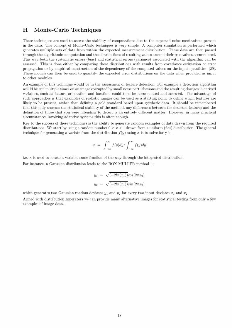
These techniques are used to assess the stability of computations due to the expected noise mechanisms presentin the data. The concept of Monte-Carlo techniques is very simple. A computer simulation is performed whichgenerates multiple sets of data from within the expected measurement distribution. These data are then passedthrough the algorithmic computation and the distributions of resulting values around their true values accumulated.This way both the systematic errors (bias) and statistical errors (variance) associated with the algorithm can beassessed. This is done either by comparing these distributions with results from covariance estimation or errorpropagation or by empirical construction of the dependency of the computed values on the input quantities [29].These models can then be used to quantify the expected error distributions on the data when provided as inputto other modules.

An example of this technique would be in the assessment of feature detection. For example a detection algorithmwould be run multiple times on an image corrupted by small noise perturbations and the resulting changes in derivedvariables, such as feature orientation and location, could then be accumulated and assessed. The advantage ofsuch approaches is that examples of realistic images can be used as a starting point to define which features arelikely to be present, rather than defining a gold standard based upon synthetic data. It should be rememberedthat this only assesses the statistical stability of the method, any differences between the detected features and thedefinition of those that you were intending to detect is an entirely different matter. However, in many practicalcircumstances involving adaptive systems this is often enough.

Key to the success of these techniques is the ability to generate random examples of data drawn from the requireddistributions. We start by using a random number 0 < x < 1 drawn from a uniform (flat) distribution. The generaltechnique for generating a variate from the distribution f(y) using x is to solve for y in

x =

∫ y0

−∞

f(y)dy/

∫

∞

−∞

f(y)dy

i.e. x is used to locate a variable some fraction of the way through the integrated distribution.

For instance, a Gaussian distribution leads to the BOX MULLER method [];

y1 =√

(−2ln(x1))cos(2πx2)

y2 =√

(−2ln(x1))sin(2πx2)

which generates two Gaussian random deviates y1 and y2 for every two input deviates x1 and x2.

Armed with distribution generators we can provide many alternative images for statistical testing from only a fewexamples of image data.

18

I Hypothesis Testing

Having made quantitative measurements from our system we will ultimately need to make decisions based uponthose measurements in comparison to some predefined model. For example, do not attempt to move the mobilevehicle through a doorway unless the vision system estimates that it will pass. Many statistical tests are based onthe idea of generating the probability that data drawn from the expected test distribution would be more frequentthan the example under test. This approach leads to the common statistical techniques of z-scores, T tests, andChi-squared tests to name a few. This follows directly from the original definition of a confidence interval, due toNeyman [18].

Such an approach to statistical analysis allows hypotheses to be tested (i.e. does the data conform to the assumedmodel?) on the basis of one model at a time, in contrast to Bayesian approaches which require all possiblegenerators (models) of the data. In addition, such statistical tests are fully quantitative. Probabilities computedfrom such statistics have the characteristic that the distribution of values drawn from the assumed model will beflat. This is useful as a mechanism for self test. The most common form of this statistic is that for a Gaussian andis known as the error function which is provided as a mathematical function in most languages (e.g. the erf()library function). The Normal Distribution (see Fig. 5) is described by the probability density function:

f(x) =1

σ√

2πe−

(x−µ)2

(2σ2) (1)

where mean = µ and variance = σ2.

Mean

2 sd’s

Figure 5: The Normal Distribution

the single sided error function is defined as

erf(x) = 2

∫ x

0

f(x) dx

However, such statistics can be generated for any model for which the expected data distribution is known, usingthe ordering principle. This states that the ordering of integration along the measurement axis should be definedso that the probability density is monotonically decreasing. For the Gaussian case shown above this gives therather trivial result that we integrate along the standard measurement axis x away from the peak, as the functionis monotonically decreasing from x = 0. We therefore use the distribution itself to define which parameter valuesare more likely to have been drawn from the model. Although this is not the only way to order the data (there arepotentially infinite numbers of equivalent possible ordering schemes depending upon how we define our variablese.g. x2) this is the one which gives confidence limits which are maximally compact in the chosen parameter domain.Generally, the preferred parameter domain would be selected as the space in which x was uniformly accurate, sothat this compactness has meaning from the point of view of measurable localisation. This is sometimes referredto as a “natural” parameterisation and is related to the concept of the equal variance transform (appendix E).

In image processing the required distributions can often be bootstrapped directly from the image (e.g. as in [6].Under these circumstances the possibility of multi-modal density functions makes the application of the orderingprinciple slightly less straightforward [5].

Finally, as the only requirement for the use of such probabilities is that they have a uniform distribution, empiricalapproaches can be used to re-flatten distributions which result from imprecise analysis. Such hypothesis tests arealso easily combined using standard statistical approaches (See appendix K).

19

J Honest Probabilities

The correct use of statistics in algorithm design should be fully quantitative. Probabilities should correspondto a genuine prediction of data frequency. From the point of view of algorithmic evaluation, if an algorithmdoes not make quantitative predictions then it is by definition untestable in any meaningful manner. Thus aclassifier giving a probability of a particular class as P should be wrong 1 − P of the time. Probabilities withthese characteristics have previously been referred to in the literature as honest [9]. The importance of this featurein relation to the work presented here is that knowledge of the expected distribution for the output provides amechanism for self-test. For example classifier error rates can be assessed as a function of probability to confirm theexpected correlation. Some approaches to pattern recognition, such as k-nearest neighbours, are almost guaranteedto be honest by construction. In addition the concept of honesty provides a very powerful way of assessing thevalidity of probabilistic approaches. In [20] it was shown that iterative probabilistic update schemes which driveprobability estimates to converge to 0 or 1 cannot be honest and are therefore also not optimal. In fact such schemesdemonstrate the common lack of quantitative rigour associated with use of psuedo-statistical methodology commonin this area. Unless computed probabilities can be shown to correspond to genuine frequencies of occurrence thenthey are of no quantitative value.

Supervised classification performance, for example object recognition, can be specified in terms of the confusionmatrix. This is table that describes the probabilities that an item of class i will be misclassified as an item of classj for each of a set of classes. The sum of each of the rows and columns should add up to 1.0.

class 1 class 2 class 3 class 4class 1 1.0 0.0 0.0 0.0class 2 0.0 0.8 0.15 0.05class 3 0.0 0.15 0.35 0.5class 4 0.0 0.05 0.5 0.45

Table 1: Confusion Matrix

A perfect classifier would have value of 1.0 along the diagonal where i = j and zero elsewhere. However, areal classifier would have some off-diagonal elements, as in this example. Note that the table is not necessarilysymmetrical. The classification algorithm might also specify a rejection rate at which it will refuse to produce avalid class output. For the probabilities delivered by a classification system to be honest, the mean probabilitygenerated for each position in the confusion matrix should agree with the relative frequency of the sampled data.For example in the table given above class 1 should always be identified with 100% classification probability.

A technology evaluation would provide an unweighted table, but a scenario evaluation would weight the entries totake account of the prior probabilities of the various objects, according to a particular application and the cost ofvarious types of error, to produce an overall number for ranking.

20

K Data Fusion

An algorithm which makes use of all available data in the correct manner must deliver an optimal result. This isnot as uncommon occurrence in computer vision as may be assumed and many problems (camera calibration forexample) do have optimal solutions [27]. If this can be established for an algorithm then extensive evaluation (e.g.on a large number of images) can be expected to prove only one thing, that the algorithm can only be betteredby one which takes account of more data or assumes a more restricted model. Use of a more restricted model willof course limit use of the algorithm, and any assumption which prevents the generic use of an algorithm needs tobe considered very carefully. It is all to easy to design algorithms which work (at least qualitatively) on a verylimited subset of images and this is a criticism which is often made of work in this area. Using more informationrather than assumptions to solve the problem might therefore be the preferred option. In a modular system, whereinput data has been separated in order to make data processing more manageable, use of more data correspondsto fusion of output data. For this reason quantitative methods of optimal data combination are of fundamentalimportance.

Optimal Combination using Covariances

Given two estimates of a set of parameters a1 and a2 and their covariances (α1 and α2) we can combine the twosets of data as follows;

aT = α−1T (α1a1 + α2a2)

with;

α−1T = α−1

1 + α−12

This method combines the data in the least squares sense, that is the approximation to the χ2 stored in thecovariance matrices has been combined directly to give the minimum of the quadratic form. The method can berewritten slightly giving

aT = a1 + α−1T α2∆a

where ∆a = a2 − a1. In this form the method is directly comparable to the information filter form of the Kalmanfilter.

Optimal Combination of Hypothesis Tests

Hypothesis test probabilities should have uniform distributions (if they are honest see appendix H). Given nquantities each having a uniform probability distribution pi=1,n, the product p =

∏n

i=1 pi can be renormalised tohave a uniform probability distribution Fn(p) using;

Fn(p) = p

n−1∑

i=0

(− ln p)i

i!(2)

Proof of this relationship can be generated in the following manner. The quantities pi can be plotted on the axes ofan n dimensional sample space, bounded by the unit hypercube. Since they are uniform, and assuming no spatialcorrelation, the sample space will be uniformly populated. Therefore, the transformation to Fn(p) such that thisquantity has a uniform probability distribution can be achieved using the probability integral transform, replacingany point in the sample space p with the integral of the volume under the contour of constant p passing throughthis point, which obeys

∏n

i=1 pi = constant. Generalisation of this process to non-integer numbers (which is usefulfor cases where we have an effective number of degrees of freedom) and other useful results are presented in [4].

Optimal Combination from Example Data

When the area of neural networks re-emerged as a popular topic in the mid 80’s much was claimed about theexpected capabilities regarding flexibility, suitability for system identification and robustness. Most of these claims

21

were subsequently shown to be optimistic. However, one problem that neural networks are relatively good at isnon-linear data fusion. A neural network when trained on an appropriate form of data with the correct algorithmwill approximate Bayes probabilities as outputs.

The mathematics describing this process is given in [14] but a more intuitive argument is as follows. Each inputvector pattern X defines a unique point in input space. Associated with each data point is the ideal requiredoutput, for example a binary output classification. As the number of samples grows large the number of examplesof data in the region of each point also grows large. If training with a least squares error function the target outputfor each point in pattern space will be the mean of local values. For a binary coding problem the mean value isthe Bayes probability of the model given the data.

Thus when using a least squares training function and training with binary class examples in the limit of an infiniteamount of data and complete freedom in the network to map any function, the network will approximate Bayesprobabilities as outputs.

Given P (A|B) and P (A|C) can we compute P (A|BC)? We can clearly solve this problem provided these prob-abilities are independent by simple multiplication. If however the measures are correlated there is no standardstatistical method for this process. This is unfortunate as we would expect a modular (AI) decision system to needto solve this task. Standard neural network architectures trained in the standard way will however approximateP (A|P (A|B)P (A|C)) for the reasons described above [2]. Provided that there is enough information in the set ofprobabilities being fused to regenerate the original data the fusion process will be able to achieve optimality.

22

L Receiver Operator Curves

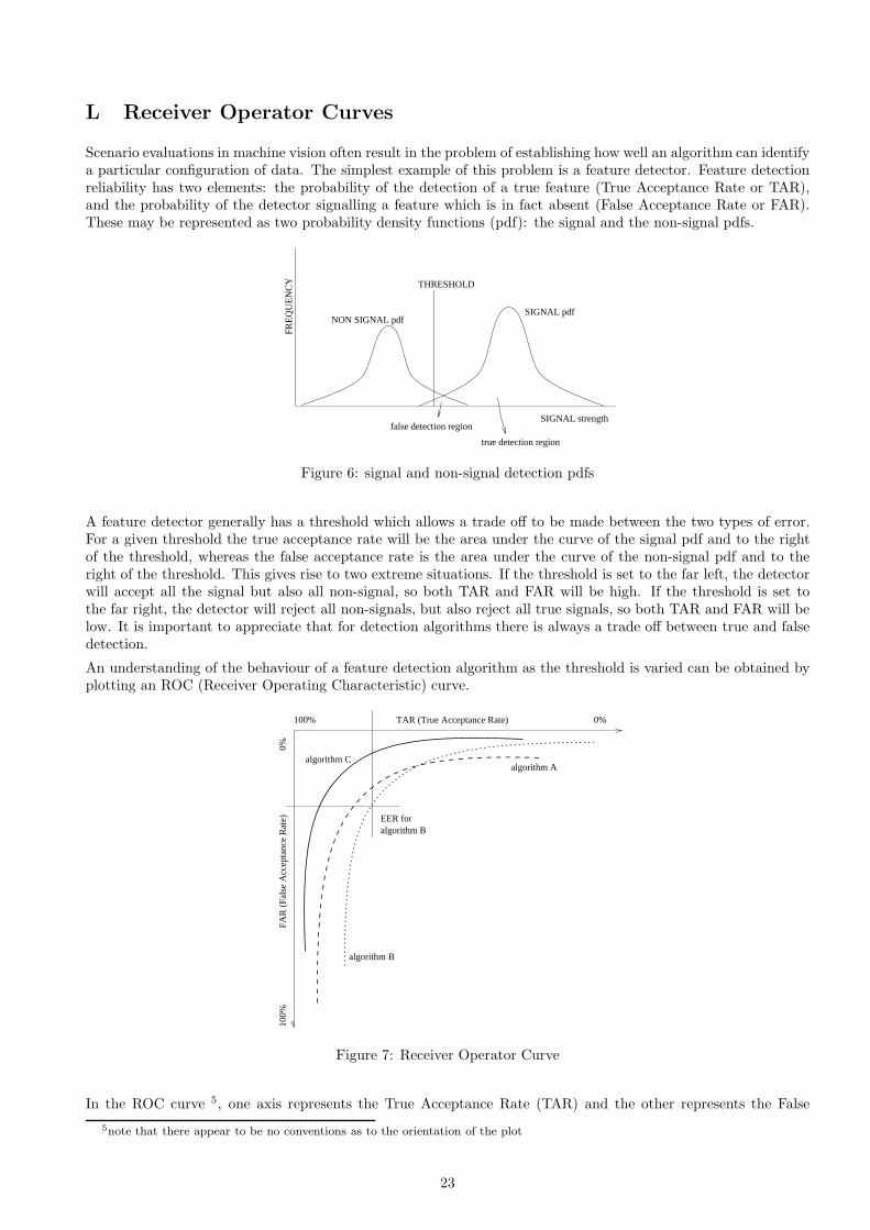
Scenario evaluations in machine vision often result in the problem of establishing how well an algorithm can identifya particular configuration of data. The simplest example of this problem is a feature detector. Feature detectionreliability has two elements: the probability of the detection of a true feature (True Acceptance Rate or TAR),and the probability of the detector signalling a feature which is in fact absent (False Acceptance Rate or FAR).These may be represented as two probability density functions (pdf): the signal and the non-signal pdfs.

THRESHOLD

NON SIGNAL pdf

SIGNAL strength

SIGNAL pdf

FRE

QU

EN

CY

true detection region

false detection region

Figure 6: signal and non-signal detection pdfs

A feature detector generally has a threshold which allows a trade off to be made between the two types of error.For a given threshold the true acceptance rate will be the area under the curve of the signal pdf and to the rightof the threshold, whereas the false acceptance rate is the area under the curve of the non-signal pdf and to theright of the threshold. This gives rise to two extreme situations. If the threshold is set to the far left, the detectorwill accept all the signal but also all non-signal, so both TAR and FAR will be high. If the threshold is set tothe far right, the detector will reject all non-signals, but also reject all true signals, so both TAR and FAR will below. It is important to appreciate that for detection algorithms there is always a trade off between true and falsedetection.

An understanding of the behaviour of a feature detection algorithm as the threshold is varied can be obtained byplotting an ROC (Receiver Operating Characteristic) curve.

TAR (True Acceptance Rate) 0%100%

FAR

(Fa

lse

Acc

epta

nce

Rat

e)0%

100%

algorithm Calgorithm A

algorithm B

EER for algorithm B

Figure 7: Receiver Operator Curve

In the ROC curve 5, one axis represents the True Acceptance Rate (TAR) and the other represents the False

5note that there appear to be no conventions as to the orientation of the plot

23

Acceptance Rate (FAR) 6. Each runs from 0% to 100%. The performance of a given detection algorithm may bedescribed in terms of a line passing through various combinations of TAR and FAR. The ideal algorithm would beone with a line that passes as close as possible to the point TAR=100% and FAR=0%. The operating point of thealgorithm along the line is determined by the setting of the threshold parameter described earlier. The setting ofthe threshold is made on the basis of the consequence of each type of error (Bayes risk), and this will depend onthe use of the results and thus the application, subject to prior probabilities of the signal and non-signal.

The performance of detection algorithms is sometimes quoted in terms of the Equal Error Rate (EER). This isthe point at which the FAR is equal to the True Reject Rate (TRR=1-TAR). This may be appropriate for someapplications in which the cost of each type of error is equal. However this is not generally the case so access to theentire ROC curve is preferred.

In contrast to the earlier pdf diagram, on an ROC diagram the performance of different algorithms may be presentedon the same plot and thus compared. In fact algorithms with completely different threshold processes may alsobe compared. For a given application (and thus TAR/FAR trade off) one algorithm may be superior to anotheraccording to the desired position along the ROC curve. For instance algorithm B may be superior to algorithm Awhen a low FAR is required. Conversely algorithm A will be preferred when a high TAR is required. AlgorithmC on the other hand provides superior performance to both algorithm A and algorithm B since for each value ofFAR, algorithm C will have a higher level of TAR.

Notice the difference between the ROC plot that presents the performance characteristics of a number of algorithms(the result of a technology evaluation), and the decision as to which is the best and how it should be tuned, whichis based on the use of this information (scenario evaluation). Of course the ROC curve is only as good as the dataused to generate it, and a curve produced using unrepresentative data can only be misleading.

There are variants of the ROC curve. If the task is to identify the features in an image, and it is possible thatthere will be more than one, then a fractional ROC (FROC) is more appropriate. This plots the total number offalse detections (since there may be more than one) against the probability of a true detection as before.

The fact that every detection algorithm involves a trade off between true and false detections has the consequencethat false detections must be tolerated by the subsequent processing stages if any reasonable level of truedetection is to be expected.

6a number of alternative forms are used such as reject rate which is (1 - acceptance rate)

24

References

1. A.P.Ashbrook, N.A.Thacker and P.I.Rockett, Pairwise Geometric Histograms. A Scaling Solution for the

Recognition of 2D Rigid Shape., Proc. for SCIA95, Uppsala, Sweden, pp271, 1995.

2. D.Booth, N.A.Thacker, M.K.Pidock and J.E.W.Mayhew. Combining the Opinions of Several Early Vision

Modules Using a Multi-Layered Perceptron. Int.Journal of Neural Networks, 2, 2/3/4, June-December, 75-79, 1991.

3. K. W. Bowyer and P. J. Phillips Empirical Evaluation Techniques in Computer Vision edited by K.W. Bowyerand P.J. Phillips, IEEE press, ISBN 0-8186-8401-1, 2000

4. P. A. Bromiley, T.F. Cootes and N.A. Thacker, Derivation of the Renormalisation Formula for the Product of

Uniform Probability Distributions and Extension to Non-Integer Dimensionality. Tina memo 2001-008.

5. P.A. Bromiley, M.L.J. Scott, M. Pokric, A.J. Lacey and N.A. Thacker, Bayesian and Non-Bayesian Proba-

bilistic Models for Magnetic Resonance Image Analysis, Submitted to Image and Vision Computing, Special Edition;The use of Probabilistic Models in Computer Vision.

6. P.A.Bromiley, N.A.Thacker and P.Courtney, Non-Parametric Subtraction Using Grey Level Scattergrams,BMVC 2000, Bristol, pp 795-804, Sept. 2000.

7. P. Courtney and N.A. Thacker, i Performance Characterisation in Computer Vision: The Role of Statistics in

Testing and Design, ”Imaging and Vision Systems: Theory, Assessment and Applications”, Jacques Blanc-Talon andDan Popescu (Eds.), NOVA Science Books, 2001, ISBN 1-59033-033-1.

8. G. Cowan Statistical Data Analysis, Oxford University Press, ISBN 0-19-850156-0, 1998.

9. A.P. Dawid, Probability Forecasting, Encyclopedia of Statistical Science 7, pp 210-218. Wiley, 1986.

10. A. Lorusso, D.W. Eggert, and R.B. Fisher, Estimating 3D Rigid Body Transformations: A Comparison of Four

Algorithms, Machine Vision Applications, 9 (5/6), 1997, pp.272-290.

11. W. Foerstner, 10 Pros and Cons Against Performance Characterisation of Vision Algorithms, Proceedings of ECCVWorkshop on Performance Characteristics of Vision Algorithms, Cambridge, UK, April 1996. Also in Machine VisionApplications, 9 (5/6), 1997, pp.215-218.

12. R.M. Haralick, Performance Characterization in Computer Vision, CVGIP-IE, 60, 1994, pp.245-249.

13. R.M. Haralick, C.N. Lee, K. Ottenberg and M. Noelle, Review and Analysis of Solutions to the Three Point

Perspective Pose Estimation Problem, Intl. J. Computer Vision, 13(3), 1994, pp.331-356.

14. M.D.Richard and R.P.Lippmann, Neural Network Classifiers Estimate Bayesian a Posterioi Probabilities, NeuralComputation,3,461-483,1991.

15. S.J. Maybank, Probabilistic Analysis of the Application of the Cross Ratio to Model Based Vision, Intl. J. ComputerVision, 16, 1995, pp.5-33.

16. D. Marr, Vision: A Computational Investigation into the Human Representation and Processing of Visual Informa-

tion Publisher W. H. Freeman Company, NY 1982.

17. P. Meer, D. Mintz, A. Rosenfield and Dong Yoom Kim Robust Regression Methods for Coputer Vision: A

Review Intl. J. Computer Vision, 6:1, 1991, pp. 59-70.

18. J. Neyman, X-Outline of a Theory of Statistical Estimation Based on the Classical Theory of Probability, Phil. Trans.Royal Soc. London, A236, pp. 333-380, 1937.

19. P. J. Phillips, A. Martin, C. L. Wilson and M. Przybocki, An Introduction to Evaluating Biometric Systems

IEEE Computer Special Issue on Biometrics, pp. 56-63, Feb. 2000.

20. I. Poole, Optimal Probabilistic Relaxation Labeling, Proc. BMVC 1990, BMVA, 1990.

21. W. H. Press, B. P., Flannery, S. A. Teukolsky and W. T. Vetterling, Numerical Recipes in C CambridgeUniversity Press., 1991

22. G. Rees, P. Greenway and D. Morray, Metrics for Image Segmentation, Proceedings of ICVS Workshop onPerformance Characterisation and Benchmarking of Vision Systems, Gran Canaria, January 1999.

23. R.S. Stephens, A Probabilistic Approach to the Hough Transform, British Machine Vision Conference BMVC90,1990.

24. A. Stuart, K. Ord and S. Arnold Kendall’s Advanced Theory of Statistics Vol. 2A, Classical Inference and theLinear Model, Sixth Edition, Arnold Publishers, 1999.

25. http://www.ti.com/sc/docs/products/index.htm Texas Instruments Semiconductor Product Datasheets TexasInstruments Incorporated.

26. http://www.tina-vision.net/ TINA: Open Source Image Analysis Environment ISBE, University of Manchester,UK

27. N A Thacker and J E W Mayhew, Optimal Combination of Stereo Camera Calibration from Arbitrary Stereo

Images Image and Vision Computing, Vol. 9 No. 1, pp. 27-32, 1991.

25

28. N. A. Thacker, F. J. Aherne and P. I. Rockett, The Bhattacharyya Metric as an Absolute Similarity Measure

for Frequency Coded Data, Kybernetika, Vol. 32 No. 4, pp. 1-7, 1997

29. P. Courtney, N.A.Thacker and A.Clark, Algorithmic Modelling for Performance Evaluation, Machine Visionand Applications, 9, 219-288, 1997.

30. N.A.Thacker and A.J.Reader, Modal Division and its Application to Medical Image Analysis, Proc. MIUA, pp7-10, London. 10th-11th July, 2000.

31. P. Viola, Alignment by Maximisation of Mutual Information M.I.T. PhD Thesis, 1995.

32. N. Wiener, Extrapolation, Interpolation and Smoothing of Stationary Time Series with an Appendix by N. Levinson

Technology Press of the MIT and J. Wiley, New York, 1949.

Questions and Answers

Comments and questions on the document accumulated following tutorials and discussions over the last two years.

Chris Taylor: Don’t you think that your methodology is too prescriptive and might stifle originality

in research?

We hope not, we are not saying anything about how people design their algorithms, only how to interpret themfrom a statistical viewpoint, and what is needed to make them useful to others. Hopefully this will just mean thatany ideas researchers have will be better developed. We would like to eliminate the cycle of people believing theyhave invented another substitute for statistics and probability, only to find later that they haven’t. Understandingconventional approaches to begin with should help researchers to identify genuine novelty.

Chris Taylor and Tim Cootes: Wouldn’t this tutorial document be easier to understand if you

included examples?

Yes it would. But as there are many possible design paths for statistical testing and we would need many examplesto demonstrate all of it. The document would get very long and people probably wouldn’t find time to read it. Wehave cited relevant papers for all aspects of the methodology and intend to produce two detailed studies, one onthe use of “mutual information” for medical image co-registration and the other on location of 3D objects usingimage features (Tina memos 2003-005 and 2005-006). Both take the approach of explicitly relating the theoreticalconstruction to likelihood and estimating covariances, followed by quantitative testing. These look like they willbe sizeable documents in themselves.

Adrian Clarke: Is it right to say that all algorithms can be related to the limited number of theo-

retical statistical methods that you suggest? This wouldn’t seem to be obvious from the literature.

As far as we can see they can, it’s just that people don’t do it. You can take any algorithm which has a definedoptimisation measure and relate the computational form to likelihood, and you can take any algorithm that appliesa threshold and relate it to hypothesis tests or Bayes theory. In the process you will find the assumptions necessaryin order to achieve this and you are then faced with a harsh choice. Do you accept that these are the assumptionsyou are making, or have you just invented a new form of data analysis? We have only ever seen one outcome tothis.

Tim Cootes: You seem to have dismissed Bayesian approaches rather abruptly without much jus-

tification.

There seems to be an attitude among those working in our area that provided a paper has the word “Bayes” inthe title then it is beyond reproach. We thought it was important to explain to people that our methodology didnot follow from Bayesian methods. The use of likelihood and hypothesis tests for quantitative analysis of data is aproven self standing theoretical framework. Allowing people to think that using Bayes fixes everything might allowpeople with this view to be dismissive of the methodology. The reasons why we say that it is difficult to makeBayes approaches quantitative are explained in detail with worked examples in a paper in the references (also Tinamemo 2001-014) but we really didn’t want to get into all of that here.

E. Roy Davies: You do not address the creative aspect of algorithm design at all in your methodology.

That is correct. Researchers will still need to define the problem they wish to solve and decide how they may wishto extract salient information from images in order to solve the task. This methodology just provides guidelinesfor how to identify and test the assumptions being made in a specific approach.

Paul Whelan: The methodology doesn’t address any of the broader aspects of machine vision system

construction, such as hardware, lighting and mechanical handling. All of these are important

in practical systems. What you have outlined might be better described as a methodology for

‘computer’ vision.

26

Yes. We have only concerned ourselves with the academic problem of designing computational modules whichextract useful information from images. Clearly a methodology document could also be written which coverspractical aspects of physical systems too. We hope someone takes the time to do this. We would however suggestthat what we suggest here should be the precursor to the process of hardware or system design. There is littlepoint buying (or building) acceleration hardware and then finding that it cannot do the computations necessary tosolve the processing task. In the meantime we will be more careful to use “machine vision” and “computer vision”at relevant places in the document to reflect your comment.

Henrik Christensen: Do you feel that academics will have any interest in this methodology? Isn’t

it really intended mainly for industrialists?

Although the methodology has as its primary purpose explaining what is necessary to make vision systems thatwork, and that may be seen as a leaning toward the more practical side, the main thrust of the paper is a theoreticalanalysis of the approach we should take to our research, therefore we believe that academics should be interested.An understanding of the ideas involved could improve the academic quality and value of work in the area. Thecurrent mantra of novelty and mathematical sophistication, as far as we can see, is never going to make consistentprogress (see the discussion of novelty vs. validity on our web pages). The task of building computer vision systemsis vast and will require that we can build on each other’s work.

Jim Crowley: Isn’t this just a statistics tutorial which could have been found in any statistical text

book?

Vision research is a forcing domain for statistics, many of the ideas presented here are not found easily in thestatistical literature, some of them have also been invented by us to solve specific problems. Also, you will notfind a case for the quantitative use of statistics in vision research in any text book. Most sciences already acceptthat this is the correct way to do research, only computer vision seems to take the attitude that it is acceptable toignore established analysis techniques. This was another reason for writing the document.

Alberto Broggi: Could this methodology be automated?

You may be able to procedurise some of the tests and data transformations, but the problems still need to beformulated and structured to begin with. Also, we are not suggesting that this methodology is complete, far fromit, it cannot be. There will be problems with data which we have not even encountered that will need to beaddressed. However, we believe that the appropriate route to developing solutions is quantitative statistics andtesting. Our methodology cannot eliminate the role of the vision researcher and we would not wish to.

27