AN EMPIRICAL ANALYSIS OF THE INTERACTIONS BETWEEN

ENVIRONMENTAL REGULATIONS AND ECONOMIC GROWTH

Chali Nondo1

Peter V. Schaeffer2

Tesfa G. Gebremedhin2

Jerald J. Fletcher2

RESEARCH PAPER 2010-13

Abstract:

The purpose of this research is to examine the relationship between environmental regulation and

economic growth. A four-equation regional growth model is used to analyze the simultaneous

relationships among changes in population, employment, per capita income, and

environmental regulations for the 410 counties in Appalachia. Our results reveal that initial

conditions for environmental regulation are negatively related to regional growth factors of

change in population, per capita income, and total employment. From this, we infer that the

diversion of resources from production and investment activities to pollution abatement is

inadvertently transmitted to other sectors of the economy—thereby resulting in a slow-down of

regional growth. We also find robust evidence that show that changes in environmental

regulations positively influence changes in population, total employment, and per capita income.

Thus, we parsimoniously conclude that in the long-run, environmental regulations are not

detrimental to economic growth.

Key Words: Environmental regulations, economic growth, regional growth model, Appalachia

1 Assistant Professor, College of Business Albany State University, 504 College Drive, Albany GA 31705;

cnondo@asurams.edu

2 Professors, Division of Resource Management, Davis College of Agriculture, Natural Resources and Design, West

Virginia University, P O Box 6108, Morgantown West Virginia

The authors acknowledge and appreciate the review comments of Alan Collins, Dale Colyer and Donald Lacombe .

1

1. Introduction

Following the passage of the Clean Air Act [CAA] in 19703, there have been heated

debates on the economic impacts of U.S. air quality regulations (Denison, 1979; Portney, 1981;

Bartik, 1985; Barbera and McConnell, 1986; Christainsen and Haveman, 1981). Despite

extensive study and debate, the relationship between environmental regulations and economic

growth is still not well understood. While several researchers including, List and Co (1999),

Gray and Shadbegian (1993), and Fredriksson and Millimet (2002a) find evidence that

environmental regulations negatively affect economic growth, Porter (1991) and Porter and van

der Linde (1995) argue that environmental regulations stimulate technological innovation and

this, subsequently leads to industrial growth. This view is known as the Porter hypothesis.4

Moreover, the focus of earlier studies has been exclusively on affected industries in the

manufacturing sector (Duffy-Deno, 1992; Jaffe and Palmer, 1996; List and Co, 1999). The

justification for this is that many of the environmental policies are directed at manufacturing

industries, and therefore, aggregate changes in employment, firm expansion or contraction will

directly affect polluting firms (Bartik, 1985). However, manufacturing is not isolated from the

rest of the national economy and as such, the effects of environmental regulations on

manufacturing industries may have spin-off effects on other sectors of the economy which

supply goods and services to the manufacturing sector, and consequently affect the pattern of

regional growth. To reinforce this view, Yandle (1985, p. 39) points out that the ―effects of

3 The 1970 Clean Air Act set National Ambient Air Quality Standards [NAAQS] for six major air pollutants:

tropospheric ozone (O3), total suspended particulates (TSP), carbon monoxide (CO), sulfur dioxide (SO2), nitrogen

dioxide (NO2), and lead (Pb). The CAA was first amended in 1977 and later in 1990.

4 The Porter hypothesis could work because firms complying with state and local environmental regulations will

invest in new capital equipment that improve productivity and at the same time help reduce emissions of pollutants. An improvement in air quality has an amenity value and that may also affect the pattern of economic growth (Van,

2002; Grossman and Krueger, 1995).

2

environmental regulations go far beyond the physical plant closings and worker layoffs" and that

the regional concentration of polluting industries may affect regional development.

From the foregoing discussion, it is clear that the impact of environmental regulation on

economic growth remains an open question. Cole et al. (2006) assert that this is because

environmental regulations have been treated as exogenous. In the same breath, Fredriksson and

Millimet (2002b) and Condliffe and Morgan (2009) note that the variables used as proxies for

environmental regulations introduce endogeneity bias in the estimation. This is because

environmental regulations can be endogenously determined by a number of factors such as

income, population, and employment change, including other socio-economic factors. This

suggests that an accurate representation in an econometric model must account for simultaneity

between environmental regulation and economic growth.

To this end, one unexplored area in the empirical literature is the use of structural

equations in estimating the environmental regulations-economic growth relationship. The

analyses presented in this study assume that environmental regulations are endogenous and are

jointly determined with per capita income, population, and total employment. Specifically, the

purpose of this research is to address a number of questions that have arisen concerning the

relationship between environmental regulation and economic growth. The questions are: to what

extent does environmental regulation influence regional growth patterns, and conversely, to what

extent do regional factors influence environmental regulations?

To address these questions, unlike in previous research, we assume that simultaneous

interactions exist among county changes in environmental regulations, per capita income,

population, and total employment. Thus, total employment, per capita income, population, and

environmental regulations are treated as endogenous variables and are specified in a four-

3

equation regional growth simultaneous model. We employ county attainment status of the

National Ambient Air Quality Standards [NAAQS]i as a proxy for environmental regulations,

and allow the cross-sectional variation of the attainment variable.

The motivation for specifying a four-equation simultaneous model is straightforward: 1)

assuming that environmental quality is a normal good, ceteris paribus, individuals with higher

incomes will support more stringent environmental regulations—thus, we hypothesize that

higher incomes positively influence environmental regulations; 2) changes in population and

industry concentration, including other firms‘ rent seeking activities will result in changes in

environmental quality. Thus, it is reasonable to conclude that changes in population and total

employment will positively influence the stringency of environmental regulations; and 3)

enforcement of environmental regulations will result in improved environmental quality and

make a location more attractive for households and businesses. This means that environmental

regulations may positively influence population growth, income growth, and employment growth

and vice versa.

This study contributes to the current discussion on economic impacts of environmental

regulation by using a regional growth model that takes into account the interdependences among

changes in environmental regulations, population, total employment, and per capita income at

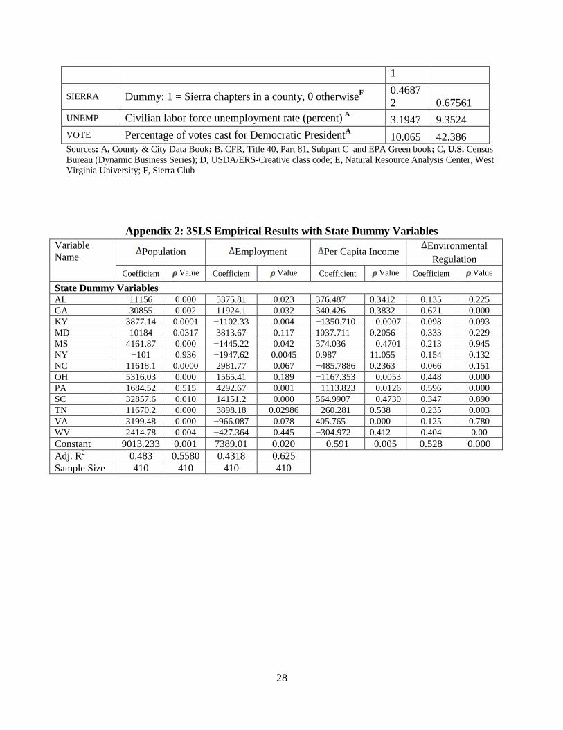
the county-level in the Appalachian Region. In order to account for state differences in growth

patterns and environmental regulation implementation, we include state dummy variables in our

empirical model. The second contribution of this study is that the empirical analyses are

extended beyond firms and industries affected by environmental regulations.

The remainder of the paper is organized as follows. Section 2 provides the analytical

framework for modeling the relationship between environmental regulations and growth, while

4

section 3 presents data sources and types. Finally, sections 4 and 5 present the results and

conclusions, respectively.

2. Analytical Framework

Within the context of the environmental Kuznets curve literature, factors such as

population density, income, industrial composition, and other socio-economic indicators have

been found to be influence the level of environmental pollution. This argument implies that

factors that influence the level of pollution also have a bearing on environmental regulation

stringency. From the concepts of utility and profit maximization, it is conceivable that consumers

and firms will respond to spatial variations in environmental quality5 (due to differences in

environmental regulation stringency) and this may consequently affect the equilibrium levels of

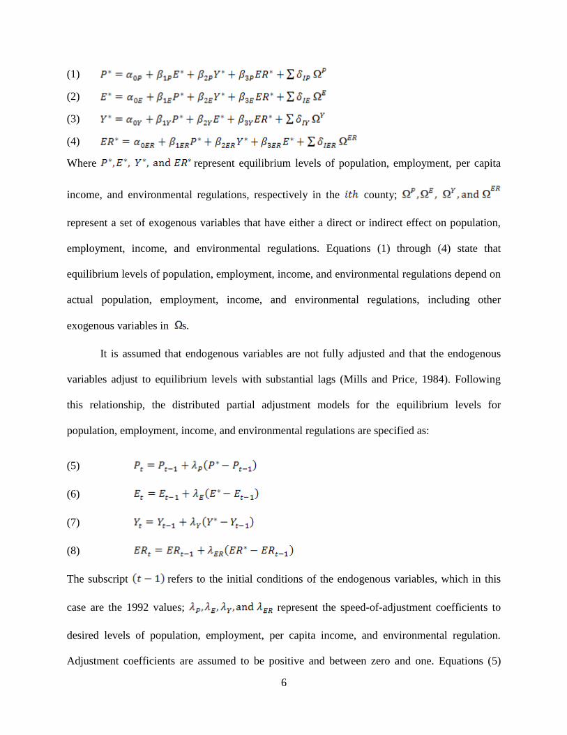
population, employment, and income growth rates across regions. These stylized facts are shown

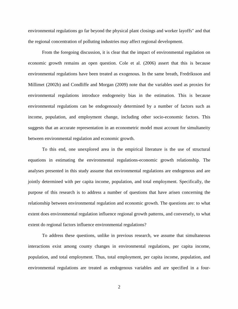
in figure 1.

According to figure 1, when environmental regulations are imposed, firms in the short-

run will incur higher production costs due to investments in abatement technologies.

Accordingly, the diversion of resources from production and investment activities will lead to

slower economic growth in terms of per capita income and employment growth. Another fact

underlying figure 1 is that in the long-run, environmental regulations enable firms to improve a

jurisdiction‘s air quality and allow firms to reduce the marginal cost of pollution control and

production, respectively. Therefore, we parsimoniously infer that the long-run gain of

environmental regulations is reduced production cost for regulated firms and improved

environmental quality. In the aggregate, environmental regulations have multiplier effects in

5 Hosoe and Naito (2006) find evidence that variations in environmental regulation implementation among and

within states have significant impacts on the mobility of capital and other resources across local jurisdictions.

Similarly, the amenities literature show that an improvement in environmental has amenity value, which in turn

helps to attract workers, businesses and wealthy retirees (Van, 2002; Grossman and Krueger, 1995; Goetz, 1996).

5

terms of attracting new firms, skilled workers, and wealthy retirees—and this also translates into

increased per capita income for a given jurisdiction.

Figure 1: Long-Run Relationship between Environmental Regulations and Regional Growth

Modified version of Goetz et al. (p. 99, 1996)

To understand the above economic impacts of environmental regulations from a regional

perspective, we extend Deller et al.‘s (2001) model by specifying a four-equation simultaneous

regional growth model. We assume that there is a lag-adjustment process between a change in

one of the endogenous variables and the other endogenous variables. In a general equilibrium

framework, population, employment, income, and environmental regulations are not only

interdependent, but will also interact with exogenous factors, including the lagged values of the

other endogenous variables.

The general form of the four-equation simultaneous model representing the interactions

among population (P), employment (E), income (Y), and environmental regulations (ER) are

specified as:

Stricter Environmental

Regulations

Better Environmental

Quality

Net Attraction of Firms

Attraction of Skilled

Workers

Increased Productivity

Attraction of Wealthy

Retirees

Higher cost/lower

output

Per capita income

[+]

Lower Production

Cost/Higher output

[+] [-]

[+]

6

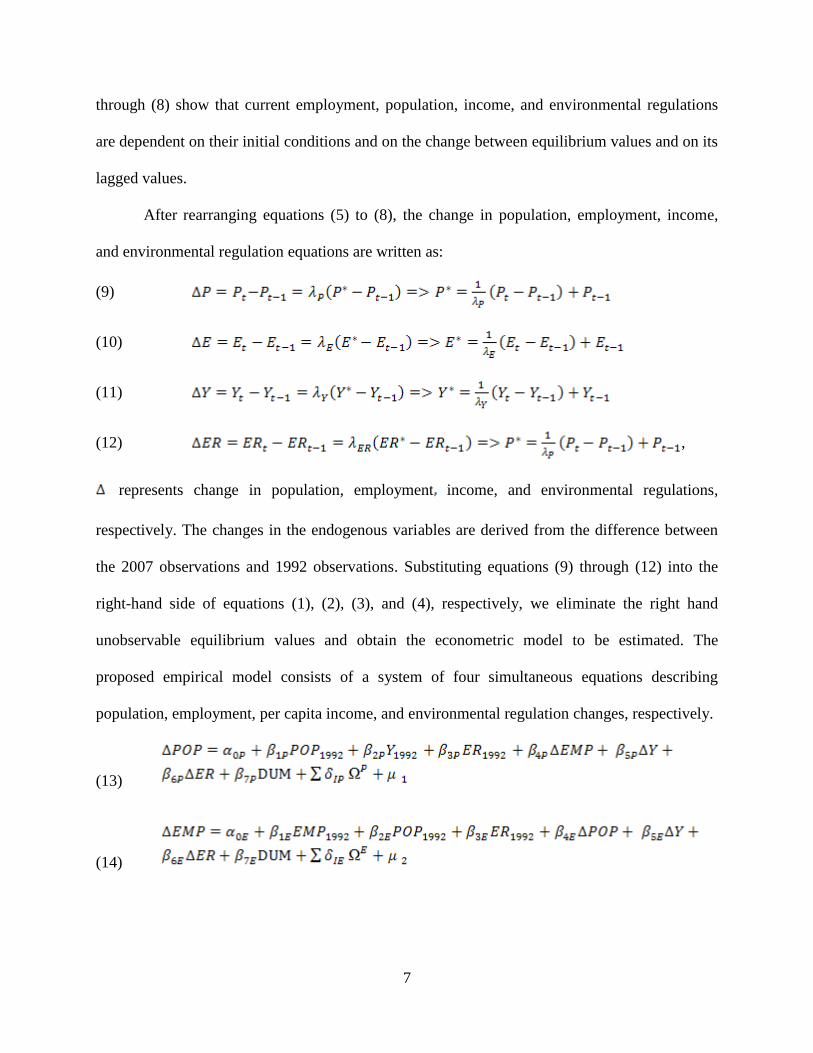
(1)

(2)

(3)

(4)

Where represent equilibrium levels of population, employment, per capita

income, and environmental regulations, respectively in the county;

represent a set of exogenous variables that have either a direct or indirect effect on population,

employment, income, and environmental regulations. Equations (1) through (4) state that

equilibrium levels of population, employment, income, and environmental regulations depend on

actual population, employment, income, and environmental regulations, including other

exogenous variables in s.

It is assumed that endogenous variables are not fully adjusted and that the endogenous

variables adjust to equilibrium levels with substantial lags (Mills and Price, 1984). Following

this relationship, the distributed partial adjustment models for the equilibrium levels for

population, employment, income, and environmental regulations are specified as:

(5)

(6)

(7)

(8)

The subscript refers to the initial conditions of the endogenous variables, which in this

case are the 1992 values; represent the speed-of-adjustment coefficients to

desired levels of population, employment, per capita income, and environmental regulation.

Adjustment coefficients are assumed to be positive and between zero and one. Equations (5)

7

through (8) show that current employment, population, income, and environmental regulations

are dependent on their initial conditions and on the change between equilibrium values and on its

lagged values.

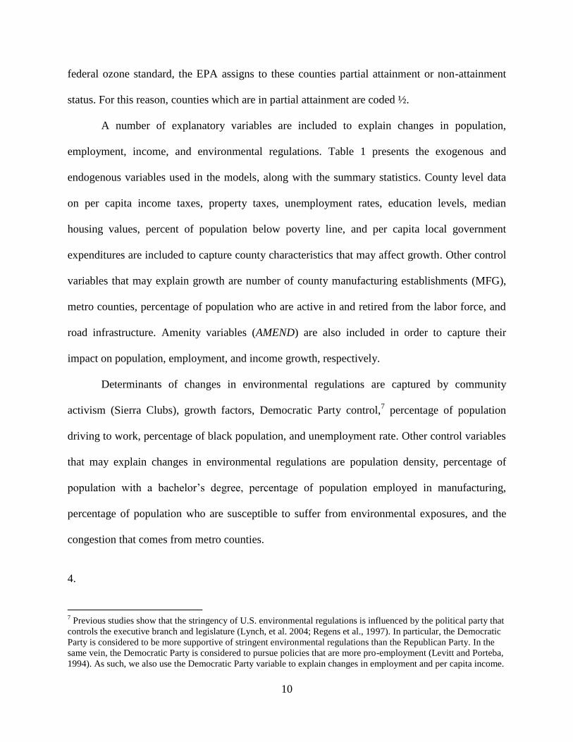
After rearranging equations (5) to (8), the change in population, employment, income,

and environmental regulation equations are written as:

(9)

(10)

(11)

(12) ,

represents change in population, employment income, and environmental regulations,

respectively. The changes in the endogenous variables are derived from the difference between

the 2007 observations and 1992 observations. Substituting equations (9) through (12) into the

right-hand side of equations (1), (2), (3), and (4), respectively, we eliminate the right hand

unobservable equilibrium values and obtain the econometric model to be estimated. The

proposed empirical model consists of a system of four simultaneous equations describing

population, employment, per capita income, and environmental regulation changes, respectively.

(13)

(14)

8

(15)

(16)

The dependent variables ∆POP, ∆EMP, ∆Y, and ∆ER denote county changes in population,

employment, per capita income, and environmental regulation, respectively; where

represent the structural error terms, is a vector of exogenous variables,

and DUM is a vector of 13 state dummy variables. 6

As already discussed, the lag adjustment

models assume that the endogenous variables do not adjust instantaneously to their equilibrium

levels but rather over a period of time. Deller et al. (2001) point out that the speed of adjustment

to equilibrium levels is embedded in the coefficients α, β, and δ. Therefore, equations (13) to

(16) estimate the short-term adjustments of population, employment, income, and environmental

regulations to their long-term equilibrium levels of (P*, E

*, Y

*, and ER

*).

3. Data

The study area is confined to the 410 counties of the Appalachian Region, which includes

all of West Virginia and parts of Alabama, Georgia, Kentucky, Maryland, Mississippi, New

York, North Carolina, Ohio, Pennsylvania, South Carolina, Tennessee, and Virginia. The data

covers the years 1992 to 2007 (Appendix 1). The dependent variables used in the models are

measured as absolute changes in population, employment, income, and environmental

regulations (1992-2007). County-level data for population, employment, and income are

obtained from the Bureau of Economic Analysis, Regional Economic Information System

6 13 state dummy variables are included as explanatory variables to capture the effect of state differences in

environmental regulation implementation and to capture the state influence on economic growth.

9

(REIS) and County and City Data Book (C&CDB) covering the years 1992 to 2007. County

attainment status is used as a proxy for environmental regulation stringency and the data is

obtained from the Federal Code of Regulations, Title 40, part 81, subpart C, covering the years

1992 to 2007.

Attainment status of a county is an appealing proxy for environmental regulation

stringency because air quality problems result from stationary pollution sources such as power

plants, factories, farming, heating of buildings, as well as cars, buses, and other mobile sources.

Together, these sources represent production and consumption activities that contribute to

environmental degradation. It can also be argued that county attainment status is an appropriate

measure for environmental regulation stringency because its enforcement is felt by the county‘s

households and firms; therefore, the analysis of such impacts must be made at county-level

(Greenstone, 2002).

Given that a county can be out-of-attainment with respect to several air pollutants, the

environmental regulation variable is an index of the total number of pollutants for which a

county is out-of-attainment. The environmental regulation index is constructed using

Henderson‘s (1997) methodology of summing the number of criteria pollutants a county is out-

of-attainment. The criteria pollutants considered are ozone (O3), sulfur dioxide (SO2), carbon

monoxide (CO), lead (Pb), and total suspended particulates (TSP). Following Henderson (1997)

and List (2001), the attainment variable takes on values from 0 (cleanest county and least

regulated) to 5 (dirtiest and most regulated)—and generally depends on the number of pollutants

the county is out-of-attainment. For example, a county in attainment for five criteria pollutants

takes on a value of 0, whereas a county out-of-attainment in all five criteria pollutants will be

coded 5. With regard to the ozone standard, when part of the county has not met the complete

10

federal ozone standard, the EPA assigns to these counties partial attainment or non-attainment

status. For this reason, counties which are in partial attainment are coded ½.

A number of explanatory variables are included to explain changes in population,

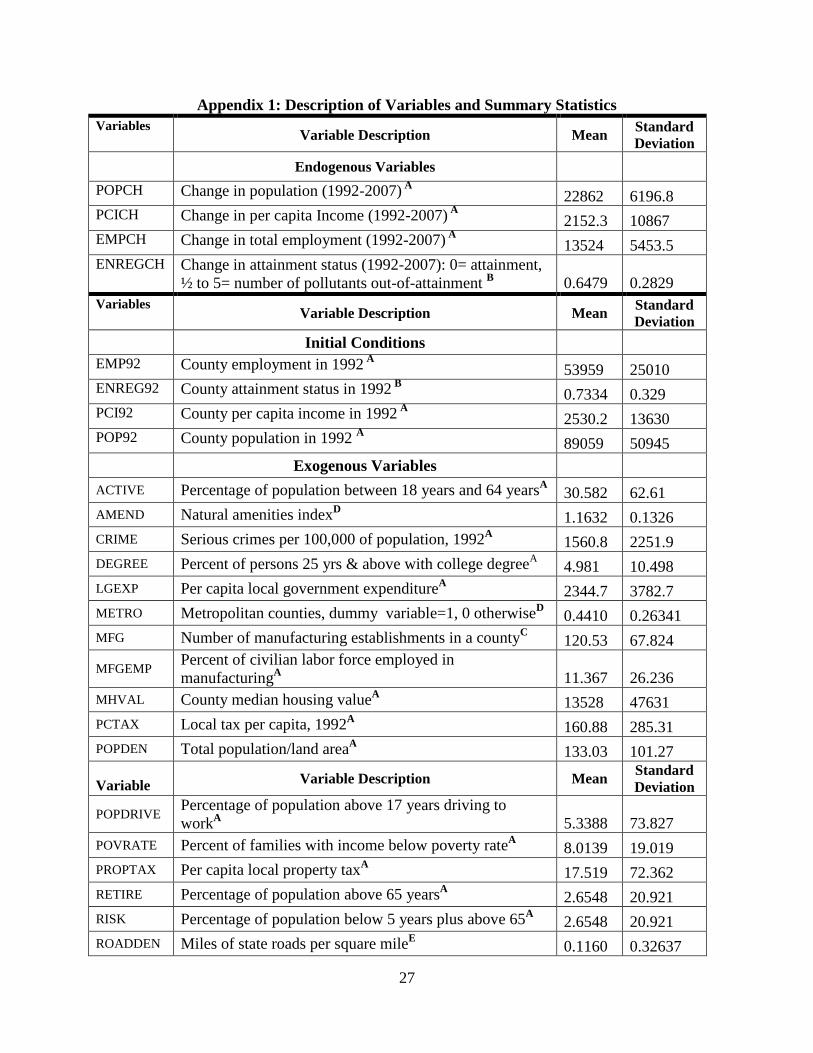
employment, income, and environmental regulations. Table 1 presents the exogenous and

endogenous variables used in the models, along with the summary statistics. County level data

on per capita income taxes, property taxes, unemployment rates, education levels, median

housing values, percent of population below poverty line, and per capita local government

expenditures are included to capture county characteristics that may affect growth. Other control

variables that may explain growth are number of county manufacturing establishments (MFG),

metro counties, percentage of population who are active in and retired from the labor force, and

road infrastructure. Amenity variables (AMEND) are also included in order to capture their

impact on population, employment, and income growth, respectively.

Determinants of changes in environmental regulations are captured by community

activism (Sierra Clubs), growth factors, Democratic Party control,7 percentage of population

driving to work, percentage of black population, and unemployment rate. Other control variables

that may explain changes in environmental regulations are population density, percentage of

population with a bachelor‘s degree, percentage of population employed in manufacturing,

percentage of population who are susceptible to suffer from environmental exposures, and the

congestion that comes from metro counties.

4.

7 Previous studies show that the stringency of U.S. environmental regulations is influenced by the political party that

controls the executive branch and legislature (Lynch, et al. 2004; Regens et al., 1997). In particular, the Democratic

Party is considered to be more supportive of stringent environmental regulations than the Republican Party. In the

same vein, the Democratic Party is considered to pursue policies that are more pro-employment (Levitt and Porteba,

1994). As such, we also use the Democratic Party variable to explain changes in employment and per capita income.

11

5. Empirical Results and Analyses

The focus of this study is on the relationship between environmental regulations and

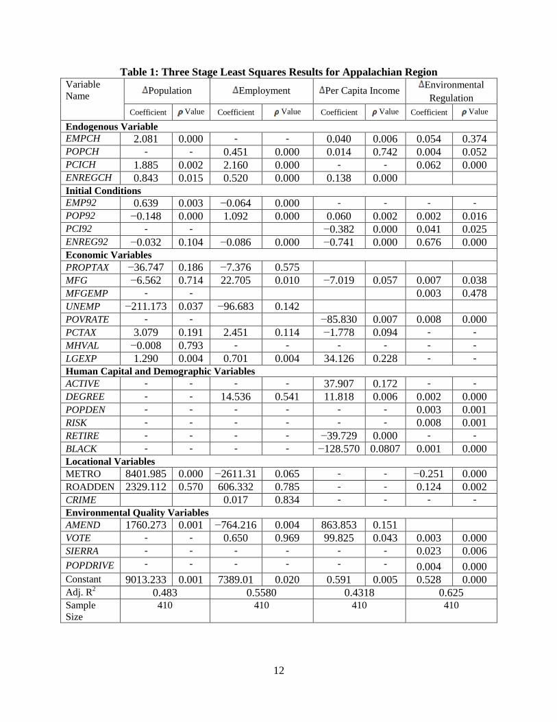
economic growth. Table 1 presents estimated coefficients of the equations based on three-stage

least squares (3SLS) estimation. The regression results reported exclude state dummy variables.8

Based on the adjusted R2 statistics, the estimated models explain 48 percent, 55 percent, 43

percent, and 62 percent of variations in changes in population, employment, per capita income,

and environmental regulations, respectively.

4.1 Change in Population Equation

Except for environmental regulations, all the initial conditions have a strong effect on

population growth and have the expected signs. Consistent with theory, results indicate that

initial conditions of population, employment and income play an important role in determining

population growth in the Appalachia. Notably, the coefficient estimate for the initial condition of

population (POP92) has a negative sign and is significant at 1 percent level. This finding

confirms the convergence hypothesis—which suggests that Appalachian counties which had

initial high levels of population tend to experience a lower absolute growth rate than counties

which had low levels of population in the initial period.

Another important variable that deserves attention is the change in environmental

regulations. Table 1. shows that the coefficient estimate for change in environmental regulations

(ENREGCH) has a positive impact on change in population and is statistically significant at the

10 percent level. One possible explanation may be that stringent environmental regulations result

8 Complete results with state dummy variables are shown in appendix 2. Overall, results indicate that interstate

differences in environmental regulation implementation and economic policies differentially and systematically

influence environmental regulation outcomes and the pattern of regional growth, respectively.

12

Table 1: Three Stage Least Squares Results for Appalachian Region Variable

Name Population Employment Per Capita Income

Environmental

Regulation

Coefficient Value Coefficient Value Coefficient Value Coefficient Value

Endogenous Variable

EMPCH 2.081 0.000 - - 0.040 0.006 0.054 0.374 POPCH - - 0.451 0.000 0.014 0.742 0.004 0.052 PCICH 1.885 0.002 2.160 0.000 - - 0.062 0.000 ENREGCH 0.843 0.015 0.520 0.000 0.138 0.000

Initial Conditions

EMP92 0.639 0.003 −0.064 0.000 - - - -

POP92 −0.148 0.000 1.092 0.000 0.060 0.002 0.002 0.016 PCI92 - - −0.382 0.000 0.041 0.025 ENREG92 −0.032 0.104 −0.086 0.000 −0.741 0.000 0.676 0.000

Economic Variables

PROPTAX −36.747 0.186 −7.376 0.575

MFG −6.562 0.714 22.705 0.010 −7.019 0.057 0.007 0.038

MFGEMP - - 0.003 0.478

UNEMP −211.173 0.037 −96.683 0.142

POVRATE - - −85.830 0.007 0.008 0.000

PCTAX 3.079 0.191 2.451 0.114 −1.778 0.094 - -

MHVAL −0.008 0.793 - - - - - -

LGEXP 1.290 0.004 0.701 0.004 34.126 0.228 - -

Human Capital and Demographic Variables

ACTIVE - - - - 37.907 0.172 - -

DEGREE - - 14.536 0.541 11.818 0.006 0.002 0.000

POPDEN - - - - - - 0.003 0.001

RISK - - - - - - 0.008 0.001

RETIRE - - - - −39.729 0.000 - -

BLACK - - - - −128.570 0.0807 0.001 0.000

Locational Variables

METRO 8401.985 0.000 −2611.31 0.065 - - −0.251 0.000

ROADDEN 2329.112 0.570 606.332 0.785 - - 0.124 0.002

CRIME 0.017 0.834 - - - -

Environmental Quality Variables

AMEND 1760.273 0.001 −764.216 0.004 863.853 0.151

VOTE - - 0.650 0.969 99.825 0.043 0.003 0.000

SIERRA - - - - - - 0.023 0.006

POPDRIVE - - - - - - 0.004 0.000 Constant 9013.233 0.001 7389.01 0.020 0.591 0.005 0.528 0.000 Adj. R

2 0.483 0.5580 0.4318 0.625

Sample

Size

410 410 410 410

13

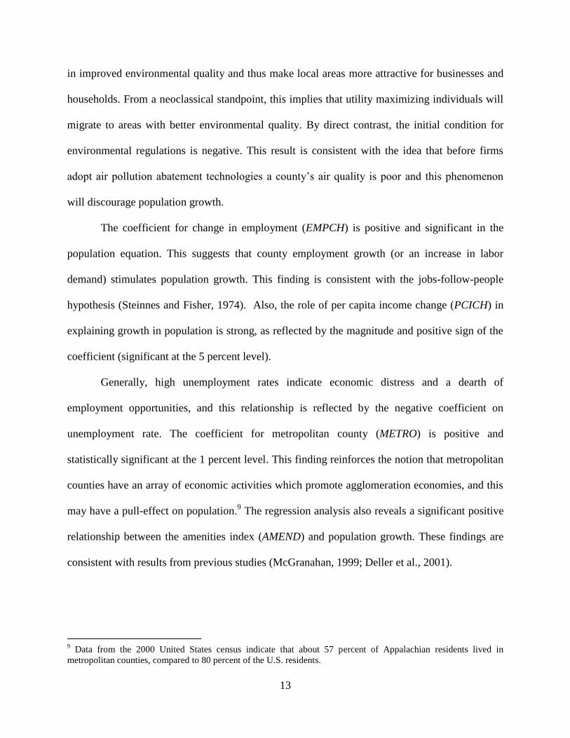
in improved environmental quality and thus make local areas more attractive for businesses and

households. From a neoclassical standpoint, this implies that utility maximizing individuals will

migrate to areas with better environmental quality. By direct contrast, the initial condition for

environmental regulations is negative. This result is consistent with the idea that before firms

adopt air pollution abatement technologies a county‘s air quality is poor and this phenomenon

will discourage population growth.

The coefficient for change in employment (EMPCH) is positive and significant in the

population equation. This suggests that county employment growth (or an increase in labor

demand) stimulates population growth. This finding is consistent with the jobs-follow-people

hypothesis (Steinnes and Fisher, 1974). Also, the role of per capita income change (PCICH) in

explaining growth in population is strong, as reflected by the magnitude and positive sign of the

coefficient (significant at the 5 percent level).

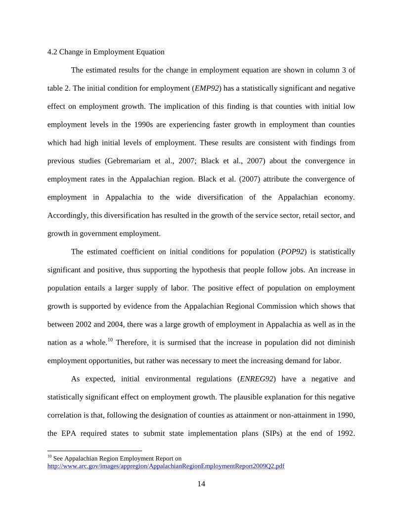
Generally, high unemployment rates indicate economic distress and a dearth of

employment opportunities, and this relationship is reflected by the negative coefficient on

unemployment rate. The coefficient for metropolitan county (METRO) is positive and

statistically significant at the 1 percent level. This finding reinforces the notion that metropolitan

counties have an array of economic activities which promote agglomeration economies, and this

may have a pull-effect on population.9 The regression analysis also reveals a significant positive

relationship between the amenities index (AMEND) and population growth. These findings are

consistent with results from previous studies (McGranahan, 1999; Deller et al., 2001).

9 Data from the 2000 United States census indicate that about 57 percent of Appalachian residents lived in

metropolitan counties, compared to 80 percent of the U.S. residents.

14

4.2 Change in Employment Equation

The estimated results for the change in employment equation are shown in column 3 of

table 2. The initial condition for employment (EMP92) has a statistically significant and negative

effect on employment growth. The implication of this finding is that counties with initial low

employment levels in the 1990s are experiencing faster growth in employment than counties

which had high initial levels of employment. These results are consistent with findings from

previous studies (Gebremariam et al., 2007; Black et al., 2007) about the convergence in

employment rates in the Appalachian region. Black et al. (2007) attribute the convergence of

employment in Appalachia to the wide diversification of the Appalachian economy.

Accordingly, this diversification has resulted in the growth of the service sector, retail sector, and

growth in government employment.

The estimated coefficient on initial conditions for population (POP92) is statistically

significant and positive, thus supporting the hypothesis that people follow jobs. An increase in

population entails a larger supply of labor. The positive effect of population on employment

growth is supported by evidence from the Appalachian Regional Commission which shows that

between 2002 and 2004, there was a large growth of employment in Appalachia as well as in the

nation as a whole.10

Therefore, it is surmised that the increase in population did not diminish

employment opportunities, but rather was necessary to meet the increasing demand for labor.

As expected, initial environmental regulations (ENREG92) have a negative and

statistically significant effect on employment growth. The plausible explanation for this negative

correlation is that, following the designation of counties as attainment or non-attainment in 1990,

the EPA required states to submit state implementation plans (SIPs) at the end of 1992.

10

See Appalachian Region Employment Report on

http://www.arc.gov/images/appregion/AppalachianRegionEmploymentReport2009Q2.pdf

15

Therefore, between 1990 and 1992 polluting firms faced stringent standards with regard to

pollution control and thus shows that stringent environmental regulations negatively affect

employment growth in the initial years of implementation due to the fact that polluting firms

have to install expensive pollution abatement control equipment. The effect of this may

inadvertently be transmitted to other sectors of the economy, thereby resulting in the overall

slow-down of total employment growth.

On the other hand, the coefficient on the change in environmental regulations

(ENREGCH) is positive and statistically significant at the 1 percent level. These results

underscore the Porter hypothesis by indicating that firms‘ marginal costs of abatement and

production may decrease over time as firms invest in efficient technology. The efficient

technology firms invest in serves the dual role of improving productivity and enhancing

environmental quality, such that areas with better environmental quality become important

locations for business investment.11

These finding are consistent with previous studies (Goetz et

al. 1996; Porter and van der Linde, 1995; Ringquist, 1993) in revealing that the short-run effects

of environmental regulation are reduced employment growth, but in the long-run environmental

regulation positively influences employment growth.

Also, the coefficient on the change in population (POPCH) is statistically significant at

the 1 percent level and is positively related to employment growth. This finding, again, confirms

the ―people-follow-jobs‖ hypothesis of Steinnes and Fisher (1974). Similarly, a change in per

capita income (PCICH) is statistically significant at the 1 percent level and is positively related

to employment growth. This means that Appalachian counties with high income experienced

11

If we assume that an improvement in environmental quality has an amenity value, it is expected that firms and

individuals will migrate to these regions, thereby stimulate growth in employment.

16

increased growth in employment. This could be attributed to the economy-wide diversification

that has taken place in the Appalachia.

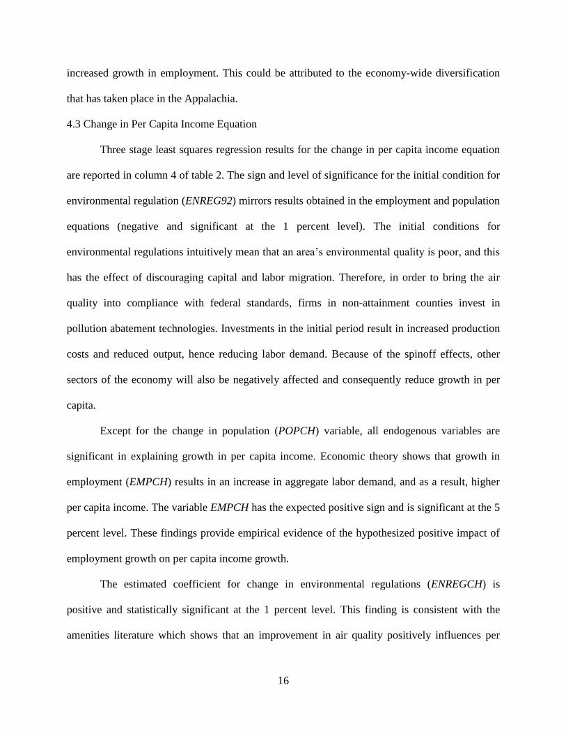
4.3 Change in Per Capita Income Equation

Three stage least squares regression results for the change in per capita income equation

are reported in column 4 of table 2. The sign and level of significance for the initial condition for

environmental regulation (ENREG92) mirrors results obtained in the employment and population

equations (negative and significant at the 1 percent level). The initial conditions for

environmental regulations intuitively mean that an area‘s environmental quality is poor, and this

has the effect of discouraging capital and labor migration. Therefore, in order to bring the air

quality into compliance with federal standards, firms in non-attainment counties invest in

pollution abatement technologies. Investments in the initial period result in increased production

costs and reduced output, hence reducing labor demand. Because of the spinoff effects, other

sectors of the economy will also be negatively affected and consequently reduce growth in per

capita.

Except for the change in population (POPCH) variable, all endogenous variables are

significant in explaining growth in per capita income. Economic theory shows that growth in

employment (EMPCH) results in an increase in aggregate labor demand, and as a result, higher

per capita income. The variable EMPCH has the expected positive sign and is significant at the 5

percent level. These findings provide empirical evidence of the hypothesized positive impact of

employment growth on per capita income growth.

The estimated coefficient for change in environmental regulations (ENREGCH) is

positive and statistically significant at the 1 percent level. This finding is consistent with the

amenities literature which shows that an improvement in air quality positively influences per

17

capita income growth (Grossman and Krueger, 1995; Goetz et al., 1996). To this end, we

parsimoniously interpret the initial conditions of environmental regulations as the short-run

effects of environmental regulations due to the fact that in the initial period, firms in non-

attainment regions invest in pollution abatement technologies. By contrast, we interpret the

change in environmental regulations as long-run effects.

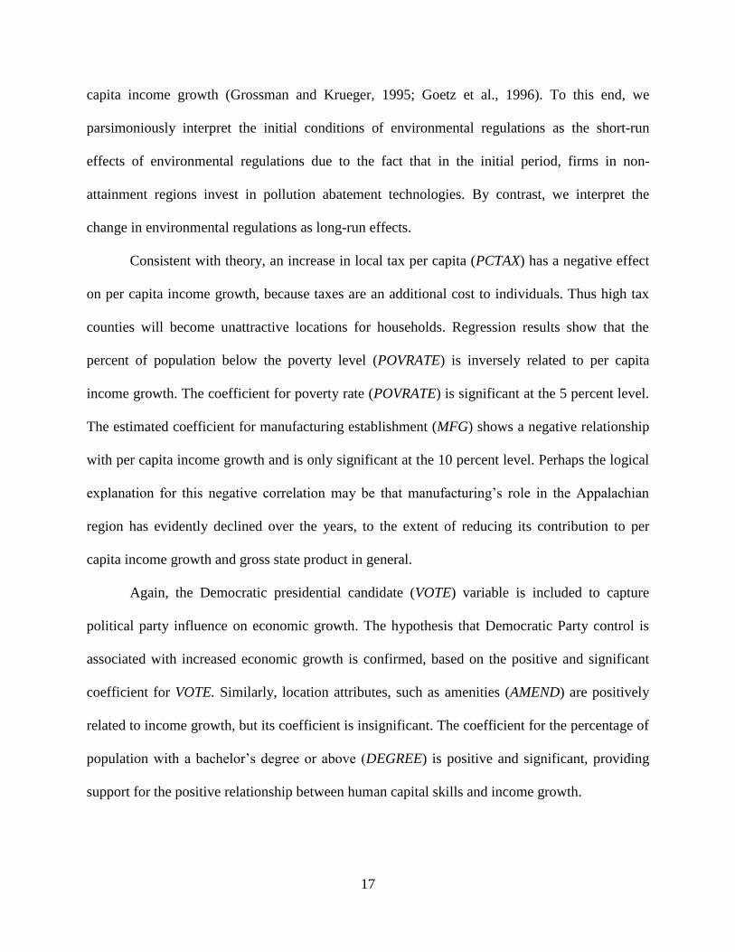
Consistent with theory, an increase in local tax per capita (PCTAX) has a negative effect

on per capita income growth, because taxes are an additional cost to individuals. Thus high tax

counties will become unattractive locations for households. Regression results show that the

percent of population below the poverty level (POVRATE) is inversely related to per capita

income growth. The coefficient for poverty rate (POVRATE) is significant at the 5 percent level.

The estimated coefficient for manufacturing establishment (MFG) shows a negative relationship

with per capita income growth and is only significant at the 10 percent level. Perhaps the logical

explanation for this negative correlation may be that manufacturing‘s role in the Appalachian

region has evidently declined over the years, to the extent of reducing its contribution to per

capita income growth and gross state product in general.

Again, the Democratic presidential candidate (VOTE) variable is included to capture

political party influence on economic growth. The hypothesis that Democratic Party control is

associated with increased economic growth is confirmed, based on the positive and significant

coefficient for VOTE. Similarly, location attributes, such as amenities (AMEND) are positively

related to income growth, but its coefficient is insignificant. The coefficient for the percentage of

population with a bachelor‘s degree or above (DEGREE) is positive and significant, providing

support for the positive relationship between human capital skills and income growth.

18

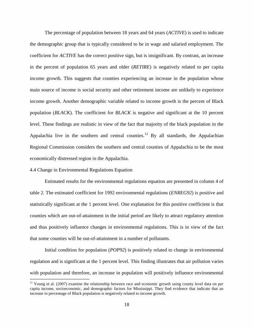
The percentage of population between 18 years and 64 years (ACTIVE) is used to indicate

the demographic group that is typically considered to be in wage and salaried employment. The

coefficient for ACTIVE has the correct positive sign, but is insignificant. By contrast, an increase

in the percent of population 65 years and older (RETIRE) is negatively related to per capita

income growth. This suggests that counties experiencing an increase in the population whose

main source of income is social security and other retirement income are unlikely to experience

income growth. Another demographic variable related to income growth is the percent of Black

population (BLACK). The coefficient for BLACK is negative and significant at the 10 percent

level. These findings are realistic in view of the fact that majority of the black population in the

Appalachia live in the southern and central counties.12

By all standards, the Appalachian

Regional Commission considers the southern and central counties of Appalachia to be the most

economically distressed region in the Appalachia.

4.4 Change in Environmental Regulations Equation

Estimated results for the environmental regulations equation are presented in column 4 of

table 2. The estimated coefficient for 1992 environmental regulations (ENREG92) is positive and

statistically significant at the 1 percent level. One explanation for this positive coefficient is that

counties which are out-of-attainment in the initial period are likely to attract regulatory attention

and thus positively influence changes in environmental regulations. This is in view of the fact

that some counties will be out-of-attainment in a number of pollutants.

Initial condition for population (POP92) is positively related to change in environmental

regulation and is significant at the 1 percent level. This finding illustrates that air pollution varies

with population and therefore, an increase in population will positively influence environmental

12

Young et al. (2007) examine the relationship between race and economic growth using county level data on per

capita income, socioeconomic, and demographic factors for Mississippi. They find evidence that indicate that an

increase in percentage of Black population is negatively related to income growth.

19

regulations stringency. However, the magnitude of the population coefficient is very small. The

coefficient for the 1992 per capita income (PCI92) is positive—reinforcing the hypothesis that

an increase in income increases the demand for environmental quality, assuming that

environmental quality is a normal good. The variable for change in per capita income (PCICH)

has a positive effect on environmental regulation change (table 2), lending support to the theory

that at high income levels, the policy response towards environmental degradation is stronger.

While the coefficient for population change (POPCH) is negative and statistically significant at

the 10 percent, the coefficient for change in employment (EMPCH) fails to attain any statistical

significance.

The EPA considers children below 5 years and adults above 65 years to be particularly

sensitive to exposure to air pollutants. The percentage of the population who are considered

sensitive (RISK) to environmental exposures has the expected positive sign. Ceteris paribus, an

increase in the proportion of the sensitive group of people will result in an increase in the

demand for stringent environmental regulations. Conceivably, community/public activism

towards environmental issues will not only emanate from the population that is susceptible to

illnesses due to environmental exposure, but will also come from environmental pressure groups,

such as the Sierra Club and others. The coefficient estimate for Sierra Club (SIERRA) is positive

and significant at the 5 percent level. These results provide evidence that environmental pressure

groups are pro-environment and will exert pressure on regulatory agencies for enforcement of

stringent environmental regulations.

Previous studies also show that the stringency of U.S. environmental regulations is

influenced by the political party that controls the executive branch and legislature (Hay et al.

1996; Lynch, et al., 2004; Regens et al., 1997). Accordingly, the percent of votes cast for the

20

Democratic Presidential candidate (VOTE) appears to have a positive influence on environmental

regulations outcomes. This finding is in accord with Kahn and Matsusaka‘s (1997) finding that

Democratic Presidential voting patterns explain environmental outcomes. Additional information

on the support for environmental regulation is provided by the positive and significant

coefficient for proportion of population with a bachelor‘s degree (DEGREE). These findings

suggest that counties featuring high levels of college graduates are more prone to support

stringent environmental regulations and are likely to lobby effectively against pollution (Hackett,

2001; Kahn, 2008).

Population density (POPDEN) and percentage of population driving to work

(POPDRIVE) are included as explanatory variables to control for the congestion externalities.

The coefficients for population density and percentage of population driving to work are positive

as shown in table 2. This follows because a dense population entails increased economic activity

and also increased vehicular traffic, which both translate into increased emissions of pollutants.

Similarly, regression results indicate that state road density (ROADDEN) positively influences

changes in environmental regulation. These findings support the notion that highway expansions

have increased vehicle miles traveled and this has also resulted in increased emission of

pollutants due to changes in land use and neighborhood (Cassady, 2004). The coefficient for

manufacturing establishment (MFG) has the expected positive sign and is significant at the 10

percent level. This implies that counties with a high number of manufacturing establishments are

likely to have more pollution and thus attract more enforcement of environmental regulations.

To control for marginal exposures to pollution, we include the percent of the black

population (BLACK) and the percent below the poverty rate (POVRATE) as explanatory

21

variables for change in environmental regulations.13

Surprisingly, regression results indicate that

counties exhibiting a high percentage of the black population (BLACK) are associated with an

increase in the stringency of environmental regulations. Similarly, the coefficient estimate for

poverty rate (POVRATE) is positive and significant at the 1 percent level. These findings

contradict the widely held view in the environmental justice literature that environmental

regulations are more strictly enforced in predominantly white and affluent neighborhoods than in

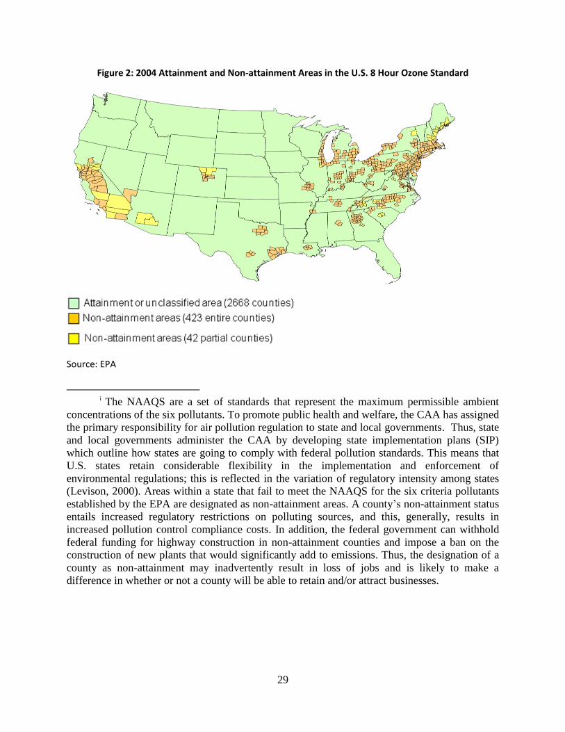
black and economically depressed neighborhoods (Melosi and Pratt, 2007). A cursory look at

figure 2 shows that in 2004 none of Mississippi‘s counties had a non-attainment designation for

the ozone standard. This is important in view of the fact that Mississippi contains the largest

number of the Black population and has the highest unemployment rates in Appalachia. These

findings corroborate Gray and Deily‘s (1995) finding that more enforcement actions are directed

towards plants located in communities with high unemployment rates. By the same token, it can

be inferred that more enforcement actions will be directed towards plants located in minority

neighborhoods in order to increase political support.

6. Conclusions and Implications

This study contributes to the body of literature by extending the analysis of the economic

growth-environmental regulation relationship beyond firms and industries directly affected by

environmental regulations. A regional growth model that takes into account the simultaneous

interactions among population, income, employment, and environmental regulations is estimated

using 3SLS. Our findings in this study can be summarized in two main propositions. First, initial

environmental regulation stringency is negatively related to regional growth factors of

13

The environmental justice literature documents that the African American and Hispanic populations are

disproportionately exposed to environmental damages than the white population. Furthermore, the literature

provides anecdotal evidence that shows that majority of polluting industrial facilities is in low income areas—

implying that people of lower socio-economic status will disproportionately suffer from environmental exposures

(Sicotte, 2009).

22

population, employment, and per capita income. The initial conditions for environmental

regulations intuitively suggest that firms in non-attainment counties invest in pollution abatement

technologies in order to bring the air quality in compliance with federal standards. To this end,

when firms initially invest in abatement capital, productivity (including labor demand) will go

down, but this will be compensated by a gradual increase in environmental quality.

Theoretically, this means that firms in the short-run will incur higher production costs due to

investments in abatement technologies, and accordingly, the diversion of resources from

production and investment activities will be inadvertently transmitted to other sectors of the

economy—and thereby retard regional growth. This finding implicitly suggests that in the short-

run there is a trade-off between environmental quality and economic growth.

Second, the empirical estimations show that change in environmental regulation is

positively associated with regional growth factors of population, employment, and per capita

income. Considering the fact that the time period for our analysis spans 15 years, we carefully

interpret change in environmental regulations as the long-run effects. Within the endogenous

growth theory framework, firms adopt improved technologies which gradually expand their

production functions as well as improve environmental quality. Within this context,

technological progress enables firms to lower the marginal cost of pollution control, and this

allows firms to produce more with less pollution. Under this assumption, the efficient technology

that firms invest in serves the dual role of improving productivity and enhancing environmental

quality. In line with the amenities literature, improved environmental quality will positively

influence firms‘ and households‘ (workers) location decisions and thus boost economic growth

in terms of growth in population, income, and employment, respectively.

23

Like in previous studies, we find evidence that supports the hypothesis that changes in

population, employment, and per capita income are interdependent. In addition, the empirical

estimations show that socio-economic, political, and demographic characteristics influence the

stringency of environmental regulations. The findings in this study reinforce the need to design

and implement environmental regulations that stimulate economic growth and enhance

environmental quality. Another policy implication is that besides imposing stringent

environmental regulations on major polluting industries, attention needs to be paid to other

socio-economic and demographic forces that contribute to emission of pollutants.

It would be interesting for future research to quantify the impacts of spillover-effects that

emanate from the spatial heterogeneity in economic policies and environmental regulation

implementation among and within Appalachian states. Also, empirical evidence that indicates

that counties featuring high unemployment rates and high Black populations are associated with

stringent environmental regulation stringency should be interpreted with caution. Could we be

committing a type I error by inferring that poor neighborhoods are not excessively exposed to air

pollution relative to other communities? Therefore, there is a need to further investigate the

simultaneous relationship between rate of exposure to pollutants and environmental regulation

stringency.

24

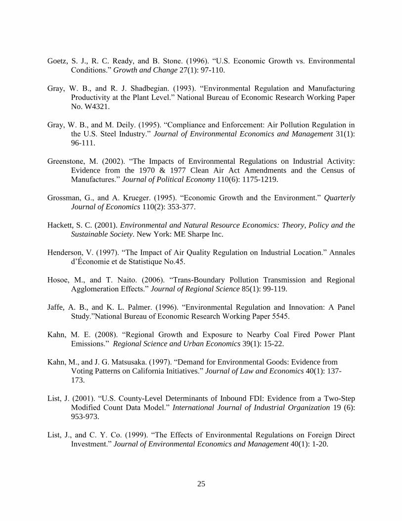
REFERENCES

Bartik, T. J. (1985). ―Business Location Decisions in the United States: Estimates of the Effects

of Unionization, Taxes, and Other Characteristics of States.‖ Journal of Business and

Economic Statistics 3(1): 14-22.

Berman, E., and L. T. M. Bui. (1998). ―Environmental Regulation and Productivity: Evidence

from Oil Refineries.‖ National Bureau of Economic Research Working Paper 6776.

Black, D. A., K. M. Pollard, and S. G. Sanders. (2007). ―The Upskilling of Appalachia: Earnings

and the Improvements of Skill Levels, 1960 to 2000.‖ Population Reference Bureau,

Washington D.C.

Cassady, A. (2004). ―More Highways, More Pollution: Road-Building and Air Pollution in

America‘s Cities.‖ U.S. PIRG Education Fund, Washington, D.C., available from

https://www.policyarchive.org/handle/10207/5542.

Cole, M. A., R. J. R. Elliot, and P. G. Fredriksson. (2006). ―Endogenous Pollution Havens: Does

FDI Influence Environmental Regulations?‖ Scandinavian Journal of Economics 108(1):

157-178.

Condliffe, S., and O. A. Morgan. (2009). ―The Effects of Air Quality Regulations on the

Location of Pollution-Intensive Manufacturing Plants.‖ Journal of Regulatory Economics

36(1): 83-93.

Deller, S. C., T. H. Tsai, D. W. Marcouiller, and D. B. K. English. (2001). ―The Role of

Amenities and Quality of Life in Rural Economic Growth.‖ American Journal of

Agricultural Economics 83(2): 352-365.

Denison, E. F. (1979). Accounting for Slower Economic Growth: The U.S. in the 1970s.

Washington, D.C.: The Brookings Institution.

Duffy-Deno, K.T. (1992). ―Pollution Abatement Expenditures and Regional Manufacturing

Activity.‖ Journal of Regional Science 32(4): 419-436.

Fredriksson, P. G., and D. L. Millimet. (2002a). ―Is There a ‗California Effect‘ in U.S.

Environmental Policymaking.‖ Regional Science and Urban Economics 32(6): 737-764.

Fredriksson, P. G., and D. L. Millimet. (2002b). ―Strategic Interaction and the Determination of

Environmental Policy across U.S. States.‖ Journal of Urban Economics 51(1): 101-122.

Gebremariam, G. H., T. G. Gebremedhin, P. V. Schaeffer, R. W. Jackson, and T. T. Phipps

(2007). ―An Empirical Analysis of Employment, Migration, Local Public Services, and

Regional Income Growth in the Appalachia.‖ West Virginia University Regional

Research Institute, Working Research Paper No. 10.

25

Goetz, S. J., R. C. Ready, and B. Stone. (1996). ―U.S. Economic Growth vs. Environmental

Conditions.‖ Growth and Change 27(1): 97-110.

Gray, W. B., and R. J. Shadbegian. (1993). ―Environmental Regulation and Manufacturing

Productivity at the Plant Level.‖ National Bureau of Economic Research Working Paper

No. W4321.

Gray, W. B., and M. Deily. (1995). ―Compliance and Enforcement: Air Pollution Regulation in

the U.S. Steel Industry.‖ Journal of Environmental Economics and Management 31(1):

96-111.

Greenstone, M. (2002). ―The Impacts of Environmental Regulations on Industrial Activity:

Evidence from the 1970 & 1977 Clean Air Act Amendments and the Census of

Manufactures.‖ Journal of Political Economy 110(6): 1175-1219.

Grossman, G., and A. Krueger. (1995). ―Economic Growth and the Environment.‖ Quarterly

Journal of Economics 110(2): 353-377.

Hackett, S. C. (2001). Environmental and Natural Resource Economics: Theory, Policy and the

Sustainable Society. New York: ME Sharpe Inc.

Henderson, V. (1997). ―The Impact of Air Quality Regulation on Industrial Location.‖ Annales

d‘Économie et de Statistique No.45.

Hosoe, M., and T. Naito. (2006). ―Trans-Boundary Pollution Transmission and Regional

Agglomeration Effects.‖ Journal of Regional Science 85(1): 99-119.

Jaffe, A. B., and K. L. Palmer. (1996). ―Environmental Regulation and Innovation: A Panel

Study.‖National Bureau of Economic Research Working Paper 5545.

Kahn, M. E. (2008). ―Regional Growth and Exposure to Nearby Coal Fired Power Plant

Emissions.‖ Regional Science and Urban Economics 39(1): 15-22.

Kahn, M., and J. G. Matsusaka. (1997). ―Demand for Environmental Goods: Evidence from

Voting Patterns on California Initiatives.‖ Journal of Law and Economics 40(1): 137-

173.

List, J. (2001). ―U.S. County-Level Determinants of Inbound FDI: Evidence from a Two-Step

Modified Count Data Model.‖ International Journal of Industrial Organization 19 (6):

953-973.

List, J., and C. Y. Co. (1999). ―The Effects of Environmental Regulations on Foreign Direct

Investment.‖ Journal of Environmental Economics and Management 40(1): 1-20.

26

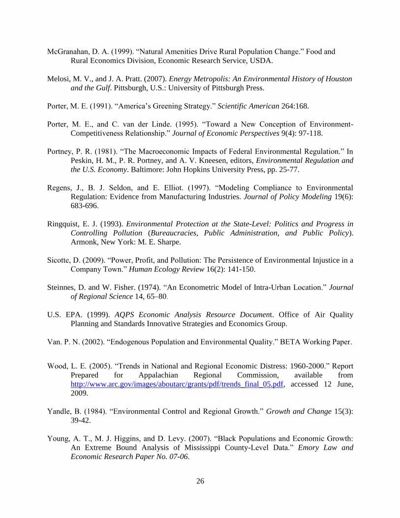
McGranahan, D. A. (1999). ―Natural Amenities Drive Rural Population Change.‖ Food and

Rural Economics Division, Economic Research Service, USDA.

Melosi, M. V., and J. A. Pratt. (2007). Energy Metropolis: An Environmental History of Houston

and the Gulf. Pittsburgh, U.S.: University of Pittsburgh Press.

Porter, M. E. (1991). ―America‘s Greening Strategy.‖ Scientific American 264:168.

Porter, M. E., and C. van der Linde. (1995). ―Toward a New Conception of Environment-

Competitiveness Relationship.‖ Journal of Economic Perspectives 9(4): 97-118.

Portney, P. R. (1981). ―The Macroeconomic Impacts of Federal Environmental Regulation.‖ In

Peskin, H. M., P. R. Portney, and A. V. Kneesen, editors, Environmental Regulation and

the U.S. Economy. Baltimore: John Hopkins University Press, pp. 25-77.

Regens, J., B. J. Seldon, and E. Elliot. (1997). ―Modeling Compliance to Environmental

Regulation: Evidence from Manufacturing Industries. Journal of Policy Modeling 19(6):

683-696.

Ringquist, E. J. (1993). Environmental Protection at the State-Level: Politics and Progress in

Controlling Pollution (Bureaucracies, Public Administration, and Public Policy).

Armonk, New York: M. E. Sharpe.

Sicotte, D. (2009). ―Power, Profit, and Pollution: The Persistence of Environmental Injustice in a

Company Town.‖ Human Ecology Review 16(2): 141-150.

Steinnes, D. and W. Fisher. (1974). ―An Econometric Model of Intra-Urban Location.‖ Journal

of Regional Science 14, 65–80.

U.S. EPA. (1999). AQPS Economic Analysis Resource Document. Office of Air Quality

Planning and Standards Innovative Strategies and Economics Group.

Van. P. N. (2002). ―Endogenous Population and Environmental Quality.‖ BETA Working Paper.

Wood, L. E. (2005). ―Trends in National and Regional Economic Distress: 1960-2000.‖ Report

Prepared for Appalachian Regional Commission, available from

http://www.arc.gov/images/aboutarc/grants/pdf/trends_final_05.pdf, accessed 12 June,

2009.

Yandle, B. (1984). ―Environmental Control and Regional Growth.‖ Growth and Change 15(3):

39-42.

Young, A. T., M. J. Higgins, and D. Levy. (2007). ―Black Populations and Economic Growth:

An Extreme Bound Analysis of Mississippi County-Level Data.‖ Emory Law and

Economic Research Paper No. 07-06.

27

Appendix 1: Description of Variables and Summary Statistics

Variables Variable Description Mean

Standard

Deviation

Endogenous Variables

POPCH Change in population (1992-2007) A

22862 6196.8 PCICH Change in per capita Income (1992-2007)

A 2152.3 10867

EMPCH Change in total employment (1992-2007) A

13524 5453.5 ENREGCH Change in attainment status (1992-2007): 0= attainment,

½ to 5= number of pollutants out-of-attainment B 0.6479 0.2829

Variables Variable Description Mean

Standard

Deviation

Initial Conditions

EMP92 County employment in 1992 A

53959 25010 ENREG92 County attainment status in 1992

B 0.7334 0.329

PCI92 County per capita income in 1992 A

2530.2 13630 POP92 County population in 1992

A 89059 50945

Exogenous Variables

ACTIVE Percentage of population between 18 years and 64 yearsA 30.582 62.61

AMEND Natural amenities indexD 1.1632 0.1326

CRIME Serious crimes per 100,000 of population, 1992A 1560.8 2251.9

DEGREE Percent of persons 25 yrs & above with college degreeA 4.981 10.498

LGEXP Per capita local government expenditureA 2344.7 3782.7

METRO Metropolitan counties, dummy variable=1, 0 otherwiseD 0.4410 0.26341

MFG Number of manufacturing establishments in a countyC 120.53 67.824

MFGEMP Percent of civilian labor force employed in

manufacturingA 11.367 26.236

MHVAL County median housing valueA 13528 47631

PCTAX Local tax per capita, 1992A 160.88 285.31

POPDEN Total population/land areaA 133.03 101.27

Variable Variable Description Mean

Standard

Deviation

POPDRIVE Percentage of population above 17 years driving to

workA 5.3388 73.827

POVRATE Percent of families with income below poverty rateA 8.0139 19.019

PROPTAX Per capita local property taxA 17.519 72.362

RETIRE Percentage of population above 65 yearsA 2.6548 20.921

RISK Percentage of population below 5 years plus above 65A 2.6548 20.921

ROADDEN Miles of state roads per square mileE 0.1160 0.32637

28

1

SIERRA Dummy: 1 = Sierra chapters in a county, 0 otherwiseF

0.4687

2 0.67561

UNEMP Civilian labor force unemployment rate (percent) A

3.1947 9.3524

VOTE Percentage of votes cast for Democratic PresidentA 10.065 42.386

Sources: A, County & City Data Book; B, CFR, Title 40, Part 81, Subpart C and EPA Green book; C, U.S. Census

Bureau (Dynamic Business Series); D, USDA/ERS-Creative class code; E, Natural Resource Analysis Center, West

Virginia University; F, Sierra Club

Appendix 2: 3SLS Empirical Results with State Dummy Variables

Variable

Name Population Employment Per Capita Income

Environmental

Regulation

Coefficient Value Coefficient Value Coefficient Value Coefficient Value

State Dummy Variables AL 11156 0.000 5375.81 0.023 376.487 0.3412 0.135 0.225

GA 30855 0.002 11924.1 0.032 340.426 0.3832 0.621 0.000

KY 3877.14 0.0001 −1102.33 0.004 −1350.710 0.0007 0.098 0.093

MD 10184 0.0317 3813.67 0.117 1037.711 0.2056 0.333 0.229

MS 4161.87 0.000 −1445.22 0.042 374.036 0.4701 0.213 0.945

NY −101 0.936 −1947.62 0.0045 0.987 11.055 0.154 0.132

NC 11618.1 0.0000 2981.77 0.067 −485.7886 0.2363 0.066 0.151

OH 5316.03 0.000 1565.41 0.189 −1167.353 0.0053 0.448 0.000

PA 1684.52 0.515 4292.67 0.001 −1113.823 0.0126 0.596 0.000

SC 32857.6 0.010 14151.2 0.000 564.9907 0.4730 0.347 0.890

TN 11670.2 0.000 3898.18 0.02986 −260.281 0.538 0.235 0.003

VA 3199.48 0.000 −966.087 0.078 405.765 0.000 0.125 0.780

WV 2414.78 0.004 −427.364 0.445 −304.972 0.412 0.404 0.00

Constant 9013.233 0.001 7389.01 0.020 0.591 0.005 0.528 0.000

Adj. R2 0.483 0.5580 0.4318 0.625

Sample Size 410 410 410 410

29

Figure 2: 2004 Attainment and Non-attainment Areas in the U.S. 8 Hour Ozone Standard

Source: EPA

i The NAAQS are a set of standards that represent the maximum permissible ambient

concentrations of the six pollutants. To promote public health and welfare, the CAA has assigned

the primary responsibility for air pollution regulation to state and local governments. Thus, state

and local governments administer the CAA by developing state implementation plans (SIP)

which outline how states are going to comply with federal pollution standards. This means that

U.S. states retain considerable flexibility in the implementation and enforcement of

environmental regulations; this is reflected in the variation of regulatory intensity among states

(Levison, 2000). Areas within a state that fail to meet the NAAQS for the six criteria pollutants

established by the EPA are designated as non-attainment areas. A county‘s non-attainment status

entails increased regulatory restrictions on polluting sources, and this, generally, results in

increased pollution control compliance costs. In addition, the federal government can withhold

federal funding for highway construction in non-attainment counties and impose a ban on the

construction of new plants that would significantly add to emissions. Thus, the designation of a

county as non-attainment may inadvertently result in loss of jobs and is likely to make a

difference in whether or not a county will be able to retain and/or attract businesses.