Eastern Illinois University Eastern Illinois University

The Keep The Keep

Masters Theses Student Theses & Publications

Spring 2021

An Empirical Analysis of Poverty and Income Inequality in U.S. An Empirical Analysis of Poverty and Income Inequality in U.S.

Southeastern States Southeastern States

Maria del Carmen Tellez Eastern Illinois University

Follow this and additional works at: https://thekeep.eiu.edu/theses

Part of the Economics Commons

Recommended Citation Recommended Citation Tellez, Maria del Carmen, "An Empirical Analysis of Poverty and Income Inequality in U.S. Southeastern States" (2021). Masters Theses. 4887. https://thekeep.eiu.edu/theses/4887

This Dissertation/Thesis is brought to you for free and open access by the Student Theses & Publications at The Keep. It has been accepted for inclusion in Masters Theses by an authorized administrator of The Keep. For more information, please contact tabruns@eiu.edu.

AN EMPIRICAL ANALYSIS OF POVERTY AND INCOME

INEQUALITY IN U.S. SOUTHEASTERN STATES

Maria del Carmen Tellez

Master’s Thesis

May 27, 2021

Supervisor: Dr. Abou-Zaid

Eastern Illinois University: Economics Department

Committee: Dr. Abou-Zaid, Dr. Moshtagh, and Dr. Abebe

Contents:

Abstract…………………………………………………………………………………...………4

Acknowledgment………………………………………………………………………...……….5

Figures…………………………………………………………………………………………….3

Tables……………………………………………………………………………………………..3

1. Introduction……………………………………………………………………………….6

2. A Brief Background on the U.S. Southeastern States………………..…………………...7

3. Literature Review………………………………………………………………………..14

3.1. Related Literature to Income Inequality and Poverty in the U.S. …..………14

3.2. Related Literature to Income Inequality and Poverty in Central America and

South America…………………………………………………………………...19

3.3. Related Literature to Income Inequality and Poverty in Western Europe..…20

3.4. Related Literature to Income Inequality and Poverty in Africa…..…………24

4. The Data and Its Properties………………………………………………………………24

4.1. The Data Set…………………………………………………………………24

4.2. The Data Properties………………………………………………………….25

5. The Empirical Analysis……………………………………………………………….….27

5.1. Methodology…………………………………………………………….…..27

5.2. The Baseline Model…………………………………………………………28

5.2.1. Model 1: Determinants of Poverty………………………………...28

5.2.2. Model 2: Determinants of Income Inequality……………………..28

5.3. The Empirical Results……………………………………………………………….28

6. Conclusion……………………………………………………………………………….33

References……………………………………………………………………………………35

Appendix A………………………………………………………………………………..…40

Figures:

Figure 1: State Income Inequality 1959………………………………………………….15

Figure 2: State Income Inequality 1989…………………………………………….……15

Figure 3: Inequality in Labor Income………………………………………………..…..23

Figure 4: Education (at least bachelor’s degree)(% of total population), by state……….42

Figure 5: Gini coefficient as a measure for household income distribution inequality, by

state……………………………………………………………………………………....42

Figure 6: Percentage of Households Led by Single Women, by state…………………...43

Figure 7: Minority Population (percentage), by state……………………………………43

Figure 8: Per Capita Personal Income, by state………………………………………….44

Figure 9: Percentage of the population over 65 years old, by state…………………...…44

Figure 10: Percentage of the Population Below Poverty Level, by state………………..45

Figure 11: Minimum Wage, by state………………………………………………….…45

Tables:

Table 1: Unit Root Test…………………………………………………………….……26

Table 2: Wooldridge Test………………………………………………………….……26

Table 3: Hausman Test…………………………………………………………………..28

Table 4: Random Effect Results for Determinants of Poverty…………………………..30

Table 5: Random Effects Results for Determinants of Income Inequality………………32

Table 6: Data description and sources……………………………………………...……40

Table 7: Expected signs of variables…………………………………………………….40

Table 8: Descriptive Statistics……………………………………………………..…….41

Abstract:

This paper analyzes the impacts of education achievement, percentage of households led

by a single parent, the percentage of minority population, per capita personal income, percentage

of population over 65 years old, and minimum wage on income inequality in 9 southeastern

states of the United States, as well as the effects of these variables on poverty, measured as the

percentage of the population below poverty level. These southeastern states are Alabama,

Arkansas, Georgia, Florida, Louisiana, Mississippi, Oklahoma, Tennessee, and South Carolina.

The period of time used for this analysis is from 2000 to 2019. Panel data was used for this

research, and two separate random effect models:

1. Model 1: Determinants of poverty

2. Model 2: Determinants of income inequality

Another important variable added to these models is a dummy variable representing the

Great Recession. The variable is defined as 0 if the period is before the Great Recession, and 1 if

the period is after the Great Recession. As we all know, the Great Recession was the largest

economic meltdown in the U.S. since the Great Depression, which lasted a little over 18 months.

The Great Recession affected GDP, which contracted steeply, and then the economy started to

grow again.

How did the Great Recession affect poverty and income inequality? The empirical results

show a positively significant relationship between the dummy variable and poverty; but seems to

be insignificant in the income inequality model.

Keywords: poverty, income inequality.

Acknowledgment:

I would like to personally express my sincere thanks to Dr. Abou-Zaid for all the

instruction, guidance, and support these past two years. He was always available to help me with

my thesis and make time for helpful feedback. Moreover, I am very grateful for all my professors

during these past six years here at Eastern Illinois University. Dr. Ali Moshtagh, Dr. Teshome

Abebe, Dr. Désiré Adom, Dr. James Bruehler, Dr. Linda Ghent, Dr. Tim Mason, and Dr. Noel

Brodsky; thank you all so very much.

I would also like to acknowledge all my classmates from 2015 until now, it has been a

long ride, but you all made these six years so enjoyable! I wish you all nothing but the best in

your future! Good luck with everything!

Finally, I would like to thank my family and friends, who stood always by my side while

completing this thesis. I am so thankful for my parents and my sister specially, for all their love,

encouragement and support sent from overseas. Without all their support I would not have been

able to achieve this.

1. Introduction:

Income inequality and poverty have been very hot topics for economists in the United

States. Inequality has been rising in America for over 20 years. Two of the income distribution

measures mostly used by economists are the Gini index and the aggregate household income

received per quintile (Bureau). In this paper the income distribution measure used is the Gini

coefficient, which lies between 0 and 1 (0 representing no income inequality, and 1 representing

high income inequality).

High poverty rates and high unemployment rates are the main reasons why young adults

are part of the rural life, especially in states like Alabama, or Arkansas. Poverty is a chronicled

unavoidable truth in numerous American rural areas. In the 1980s, there was a noticeable

economic expansion, which did not affect the high poverty rates (Deavers and Hoppe, 1992).

With this being said, it is shown that the poor are at a huge disadvantage when looking for a job,

or a higher income, even when the economy is showing economic growth.

The causes of poverty is a list that goes on and on (Duncan, 1992). The research has

shown that there is a relationship between poverty and the labor market, racial and gender

inequality, welfare support programs, households led by single parents, economic insecurity, or

low human capital.

To give public services, and to reinforce and broaden every state's economy, strategy

policy makers need to be aware of the poverty level and the idea of pay distribution designs.

Understanding the qualities of the rural poor is very important for planning explicit advancement

arrangements to lessen the reasons for poverty and ease income inequality.

This study applies Random Effect model for both models (determinants of poverty and

determinants of income inequality). Random Effects models are “statistical models in which

some of the parameters (effects) that define systematic components of the model exhibit some

form of random variation” (Salkind, 2012). The data used is over the period 2000 to 2019 for 9

American states located in the southeastern region of the country.

This paper is divided into five parts. In the first part, “Brief Background on the states”, I

give a background on all the states used on my research. In the second part, “Literature Review”,

I review the studies and research exploring the correlation between my independent variables

and poverty, and income inequality for different countries. This second part is divided into 4

sections:

- Income Inequality and Poverty in the U.S.

- Income Inequality and Poverty in Central America and South America.

- Income Inequality and Poverty in Western Europe.

- Income Inequality and Poverty in Africa.

After that, I present the data set and its properties. Thirdly, I present the empirical

analysis, where I explain the methodology, the preliminary tests, the baseline models, and the

empirical results. The final part is the conclusion, where I show a summary and concluding

remarks.

2. A Brief Background on the States:

- Alabama:

Among the 50 American states, Alabama is significantly poor, and the median family

income has stayed below the national average for decades. Alabama’s employment is mostly

focused on farm-related employment, which has actually decreased; as well as the agriculture’s

share of Alabama’s economy.

Primary and secondary education in Alabama had improved significantly in the last half

of the twentieth century, however government funded schools in the state have kept on

experiencing weak local funding coming about because of the state's low property taxes.

Educators' compensations have been rising, yet at the same time rank among the lowest in the

country. Rural schools get less help than those in metropolitan zones.

The average drop in income among the bottom 20% of households in Alabama has been a

13.5% over the last ten years; while the average increase in income among the top 20% of

households in Alabama has been 13.8%. This income inequality has been worsening since the

1970s. If we look at the income inequality by population groups, the research showed a 16.8%

increase for the poorest 20% of households; a 31.5% increase for the middle 20% of the

households in Alabama; and a 71% increase for the richest 20% of the households in Alabama.

According to the Center on Budget and Policy Priorities (2012), the richest 5% of households in

Alabama have an average income 12.8 times higher than the bottom 20% of the households, and

4.5 times larger than the middle 20% of households.

- Arkansas:

With a total population of over 3 million, the median household income in Arkansas in

2018 was $47,062; and the poverty rate was at a 17.6%. The ethnic groups in Arkansas are white

(non-Hispanic) 72.1%, black or African American (non-Hispanic) 15.1%, white (Hispanic)

4.38%, other (Hispanic) 2.66%, and two or more races (non-Hispanic) 2.54%. Females in

Arkansas have an average income ($42,470) 1.35 times lower than the average male. The income

inequality in Arkansas in 2018 was lower than the national average, measured using the Gini

coefficient; it was 0.45.

In Arkansas, 17.6% of the population lived below the poverty level, which is higher than

the national average of 13.1% in 2018. The Census Bureau uses a “set of money income

thresholds that vary by family size and composition to determine who classifies as impoverished.

If a family’s total income is less than the family’s threshold than that family and every individual

in it is considered to be living in poverty” (Arkansas, 2018).

The gross domestic product (GDP) by state, also known as gross state product (GSP), is

used to measure the output of each state’s economy each year; it is used to measure how much of

all the goods and services’ final value was created in that state. The U.S. Bureau of Economic

Analysis (BEA) shows different sectors used to measure each state’s gross state product, like

construction, retail trade, health care, or military. In the case of Arkansas, the private industry

sectors that contribute the most to the GDP are insurance, real estate, manufacturing, and

professional and business services (Economics, s.f.).

- Georgia:

Georgia is one of the states that has been raising the living standards of its population.

The economic growth of this state has been increasing from 2005 averaging a 5% increase

annually. The economy in the state of Georgia grew by 2.7% in 2016, driven mostly by

construction (The World Bank, 2021). In 2019, poverty declined to a 19.5%, almost half of

poverty rate in 2007 because of the macroeconomic policies implemented and the improved

governance. According to The World Bank data found for the state of Georgia in 2020, the total

population was 3.7 million, the GDP (measured in current US$ billion) was 15.9, the GDP per

capita (current US$) was 4,275, and the life expectancy at birth in years was 74.1.

Georgia’s GSP in 2019 reached almost $540bn, which is a growth of a 3% from 2014 to

2019 (IBISWorld, 2021). What employment trends are impacting Georgia? In 2018, the state of

Georgia employed 6.3 million people, which is a 2.7% growth rate from 2013 to 2018. The

sectors of employment mostly used in this state are health care and social assistance, retail trade,

and scientific/technical services.

According to IBISWorld, the per capita personal income, also known as DPI (disposable

personal income) is the amount of money that someone has available to use for spending or

saving after income taxes. In 2018, Georgia’s DPI was around $46,000, 37th out of all 50 states

in the U.S.

- Florida:

The data found at the U.S. Bureau of Economic Analysis for Florida’s gross domestic

product (GDP) shows a growth rate of a 4% in 2015, about 1% higher than the national average.

The next year, the growth decreased by almost 1% (3.2%), which is still above the national

average (1.6%). In 2017, the real growth decreased by 1% (2.2%), which was equal to the

national level (Bureau of Economic Analysis (U.S. Department of Commerce), 2018).

What are the economic strengths of Florida? There are many economic strengths that

help the state of Florida economically (Facts about Florida, 2013):

- International trade: being so close to Latin and South America, 40% of U.S. exports pass

through Florida.

- Tourism: in 2011, there was a record number of visitors in Florida (87.3 million). The

tourism industry has a huge economic impact on Florida’s economy; about $67 million.

- Agriculture: the southeastern states are known for its farm industry, but Florida leads all

these states. It produces over 65% of oranges in the U.S. and supplies about 40% of the

world’s orange juice.

Population growth is one of the main reasons why the state’s economic growth is

increasing, and the population over 65 years who retire in Florida have a very important impact

on it as well. The growth rate between 2020 and 2030 is expected to increase, and Florida’s older

population is expected to represent almost 57% of these gains (Florida’s Economic Future & the

Impact of Aging, 2014).

- Louisiana:

In the 1700s and 1800s, Louisiana’s economy was mainly focused on agriculture,

specially cotton in the northern counties, and sugarcane in the southern counties. In the late

1800s, lumbering began to grow and became the major part of Louisiana’s economy until the 21st

century. Nowadays, agriculture is not as important as it was to Louisiana’s economy back in the

day. Only a small percentage of the state’s population own their own farm and make a living out

of it (Economy of Louisiana, 2014).

Moreover, education in Louisiana has been at the bottom of the list of all fifty states.

Louisiana has over 20 public institutions and 10 private institutions of higher education.

Louisiana State University (LSU) is the foundation of Louisiana’s system of higher education.

Education is one of the top priorities in Louisiana today. Louisiana is a state that has always been

ranked at the bottom of the 50 states on educational quality. According to the Southwest

Educational Development Laboratory, “educational leaders in Louisiana are taking an approach

to reform that focuses on the entire educational system to ensure that change takes place in an

integrated way, rather than progressing in a piecemeal fashion. They are looking to the national

reform movement for guidance and support in improving the quality of education for all students

in the state. Teaching in Louisiana is expected to improve as teachers are given more resources,

responsibilities, and opportunities to learn new skills” (The Progress of Education in Louisiana,

1996).

- Mississippi:

There has been an outstanding improvement in employment in Mississippi since the mid-

20th century, but in the 21st century, the per capita gross product of the state was amongst the

lowest in the country. Some of the largest sectors of the state’s economy are retail trade, real

estate, and health and social services. In the 20th century, since the number of farms in

Mississippi decreased, Mississippi’s economy became not as dependent on agriculture as it used

to be. Once the 21st century began, the agriculture sector became only a tiny part of Mississippi’s

gross state product (Economy of Mississippi, 2020).

In 2019, Mississippi’s gross state product was over $104bn, which shows a growth of 0.8%

from 2015 to 2019. When comparing it to all the other U.S. states, Mississippi’s GSP growth

ranks 44th. What sectors affect Mississippi’s GDP? The main sectors that give more gross

domestic product and employ more people are manufacturing, real estate, health care and social

assistance, retail trade, finance and insurance, food services, and construction. There are many

others, but those are the main sectors that give the most gross domestic product (Mississippi -

State Economic Profile, 2019).

- Oklahoma:

Most states’ economy has been balanced, but in the case of Oklahoma, it has not always

been that way. A significant percentage of the population has been considered below poverty

level for years; the annual per capita income (also known as median household income) is

significantly below the national average. As said above, there are different sectors that give more

gross domestic product and employ more people. In Oklahoma, these sectors are retail trade,

manufacturing, finance, insurance, real estate, transportation, and construction.

Agriculture has been a very dominant part of Oklahoma’s GSP, but as years go by, the

number of farms keeps decreasing. Oklahoma’s mineral production is one of the highest in the

country. Historically, oil and gas have always been very important components of Oklahoma’s

economy (Economy of Oklahoma, 2019).

- Tennessee:

Even though Tennessee is now mostly industrial, most of the population still resides in

urban areas, where the population make a living off their land. Agriculture is a big factor in

Tennessee (cotton, tobacco, soybeans, and dairy products). Not only is agriculture important for

Tennessee’s economy, minerals are as well. The top mineral in Tennessee is stone, followed by

zinc, which production is led by Tennessee.

Tourism is a very important factor when speaking about Tennessee’s economy.

Tennessee has been a major tourist destination because of its famed music capitals, like

Nashville for its country music, or Memphis for its jazz (Tennessee: Economy, 2012).

According to the Statista Research Department, “in 2020, the real Gross Domestic

Product (GDP) of Tennessee decreased by roughly 4.9 percent compared to the previous year.

The state's real GDP experienced the most growth in 2004, when it increased by 4.9 percent

when compared to the previous year” (Annual percent change of the real GDP in Tennessee from

2000 to 2020, 2021).

- South Carolina:

The Civil War was devastating for South Carolina, both for its population as well as its

economy, but at the beginning of the 20th century, the state began to see changes. The

manufacturing sector started to provide economic relief to its workers, and with the Civil Rights

movement in the 1960s, segregation and legal discrimination ended, though racial divisions

remain a concern for South Carolina today.

South Carolina’s tourism sector has increase in the past few years with Charleston and

Myrtle Beach as two of the top East Coast vacation spots (South Carolina, 2019).

South Carolina’s GDP (Gross Domestic Product) was almost at $220 billion in 2017 (26th

in the country). In 2018, this GDP grew by 2.3%; the factors that contributed to this increase

were manufacturing, construction, professional and business services, and health care and social

assistance (South Carolina Economic Analysis Report, 2018).

3. Literature Review:

This section is divided into different sections, depending on what countries it is focused

on. Firstly, the United States, which is followed by Latin and South America, Western Europe,

and Africa.

3.1. Related Literature to Income Inequality and Poverty in the U.S.:

Income inequality has been a hot topic in the United States for over 40 years, or even as

early as the 1960s, but economists have been giving the situation more attention in the last 10

years. Southern states have been known to have a higher inequality than other states in the

United States. Most of the previous research has been focused on the determinants of state

income inequality, by using cross-sectional data analysis for a given year, even though there has

also been panel data (cross-sectional data for multiple periods of time).

William Levernier’s (1995) research on income inequality in 48 states for 1960, 1970,

1980, and 1990, showed that an increase in income inequality in the 1980s was positively related

to households led by single women or mothers, and immigrants from many foreign countries. He

measured family income inequality with the Gini coefficient, which lies between 0 and 1; the

higher the value, the higher the degree of income inequality. On his paper, he showed the

following figure; the state income inequality in 1959.

Figure 1 shows that states with the highest income inequality in 1959 were concentrated

in the Southeast. Income inequality was at its lowest in New England, the Great Lakes and the

Northwest.

The degree of income inequality in the U.S. seriously shifted between 1960 and 1990. On

the one hand, the states with high income inequality were not only concentrated in the South;

states like New York or Illinois shifted into this group. Figure 2 shows the change of income

inequality in the Unites States in 1989.

In his model, he included economic, demographic, human capital, labor market, and

regional characteristics. The results showed that in the 1980s, the factors that caused an increase

in income inequality were international migration and the households led by single females. On

the other hand, the factors that reduced income inequality were high school degree attainment,

labor-force participation, goods-producing employment share, and transfer payments.

The general literature mentions education as one of the factors that most affect income

inequality all around the globe. This mostly happens in African countries, but it is still noticeable

in the United States, where the children of the wealthy have more opportunities for educational

achievement than the children of everyone else in the country (Reardon, 2014). One of the

clearest ways of noticing the economic inequality that the United States is experiencing, is the

educational achievement gap between the children of the wealthy population and the children of

the non-wealthy population. Today, the educational gap is mostly defined by wealth and income;

more so than ethnicity or race. Back in the 1950s and 1960s, it was the other way around; racial

discrimination was the main aspect that led to inequality in the United States. But civil rights and

anti-discrimination legislation led to better economic, educational, and social conditions for

minorities in the United States of America.

Sousa-Brown (2004) analyzed the determinants of poverty and income inequality in the

rural counties of West Virginia, by using OLS and 2SLS regressions with cross-sectional county

data. The empirical results showed simultaneity between poverty and income inequality; making

poverty the main determinant of income inequality in the counties of West Virginia.

Manufacturing is another important variable when talking about income inequality. Over

the last 50 years, the United States has been through a couple trends: the increase in income

inequality, as well as The Industrial Period (1945-79), The Deindustrialization of America

(1980-2000) and then The Reindustrialization (Bolden, Clark, & Agbodzakey, 2020). Their

hypothesis was that manufacturing plays a very important role in income inequality. They

focused on the relationship between manufacturing and income inequality in the state of

Alabama, using empirical techniques. Their hypothesis was not supported since the results

indicated that manufacturing does not play a key role in income inequality.

Furthermore, their results brought us back to education being one of the most important

factors, because the more education in a community, the less income inequality. Additionally,

whether you live in a rural or urban area affects income inequality. And finally another fact that

their results proved is that counties with a high African American population tend to have a high

income inequality.

Some literature related income inequality to mortality rates, but economists question

whether this relationship does not depend on per capita income. Lochner, et al. (2001) analyzed

this issue with data from over 500,000 people in the United States, over a 8-year period; and the

Gini coefficient was used as the measurement for income inequality. The results showed that the

population living in states with high income inequality, have a higher mortality rate; while the

population living in the states with low income inequality tend to have a lower mortality rate.

They concluded that high income inequality is positively related to a high mortality rate.

Other authors tested whether the relationship between income inequality and mortality

might be different because of the level of education or not (Muller, 2002). He used a multiple

regression analysis with mortality as the dependent variable, and Gini coefficient (as a

measurement of income inequality), income per capita, and the percentage of the population over

18 years without a high school diploma as the independent variables. His data was from 1989

and 1990 for all states, including the District of Columbia. In his model, the independent variable

of most interest was the Gini coefficient for households, ranging from 0 to 1 and measuring the

level of income inequality. To control the different income levels among states, he included per

capita income in his regression model; which was in the log form to reduce positive skew. And,

since education is one of the most important factors when talking about income inequality, he

measured educational attainment as the percentage of people over 18 years old without a high

school diploma.

Firstly, he analyzed a regression model without the independent variable of population

over 18 years without a high school diploma. The results showed that income inequality’s effect

on mortality was insignificant. But, once he added that independent variable to the regression,

the fit of the regression increased significantly.

How about the elderly? A high percentage of the 65 years or older population was

projected to go into homelessness from 2010 to 2020. Usually these older adults have critical

health and housing needs which cannot be afforded (Sermons & Henry, 2010). The exposure to

extreme weather as well as other unhealthy environments in shelters can affect the wellbeing of

our elders. The mental health of the elderly is also very important when looking at the reasons

why older people end up homeless, and even stay homeless in some cases. An example could be

memory loss, an illness that can make the elderly unable to secure housing. They concluded their

research with a list of recommendations that would reduce elderly homelessness and even,

hopefully, completely eliminate it in the United States.

- The rise of subsidized housing that elderly people find reliable and affordable.

- Generate an adequate and indefinite supportive housing to completely eliminate

homelessness.

- Analysis and investigation to achieve a better understanding on what homelessness of the

elderly population is.

Tennessee is among the states with the highest income inequality along with Kentucky,

Alabama, Oklahoma, and North Carolina. According to the Center on Budget and Policy

Priorities (2012), inequality in Tennessee has worsened for over 50 years. After years of

widening inequality, Tennessee’s upper class households have incredibly bigger incomes than

the lower class households. “The richest 5% of households have average incomes 13.4 times as

large as the bottom 20% of households and 4.9 times as large as the middle 20% of households”.

3.2. Related Literature to Income inequality and Poverty in Central America and South

America:

According to OECD (2021), among the 37 OECD (Organization for Economic

Cooperation and Development) countries, the United States is top five with the highest income

inequality in 2019, with 0.39; behind Bulgaria (0.408), Mexico (0.458), Chile (0.46), and, at the

top of the list, Costa Rica (0.478). As shown above, some Latin American countries have a

relatively high income inequality, even though there has been a significant progress in reducing

it. Alberto González Pandiella (2017) analyzed income inequality in Costa Rica using an income

source decomposition approach by Lerman and Yitzhaki (1985), which allowed him to identify

the degree of contribution of any income source to income inequality (measured with the Gini

coefficient). The decomposition approach of this method is the mathematical expression where

the Gini coefficient is shown as a covariance between income and the observations in the

distribution curve.

𝐺𝑦 = ∑ 𝑆𝑘 𝑅𝑘 𝐺𝑘

According to that expression, income inequality can be decomposed into three elements:

- 𝐺𝑘 : the Gini coefficient of income source k.

- 𝑆𝑘 : the share of income source k in total income.

- 𝑅𝑘 : the Gini correlation between income source k and the total income.

In his research, Alberto González Pandiella also looked at inequality by gender, age, and

level of education. He concluded that in Costa Rica, income inequality is higher for the youngest

and the oldest population. This is because the youngest population has a student status, and the

oldest population has a retired status. When looking at income inequality per gender, he observed

that inequality is higher for women than it is for men. In the case of Costa Rica, women are more

likely to be poor, or unemployed; therefore they are more likely to be recipients of social

assistance programs.

The immigrant population in Costa Rica keeps increasing, specially from Nicaragua.

According to Alberto González Pandiella (2017), in 2013, 10% of the population employed were

foreign. Immigrants in Costa Rica tend to be low qualified, and women unemployment rates are

extremely high, almost double of native women unemployment.

Costa Rica is very committed to its investment in education; but educational gaps are still

very noticeable because of someone’s socioeconomic status. People with no education or low

levels of education have the largest inequality; while the population with technical secondary,

tertiary, or graduate higher education have the lowest inequality. This suggests that the more

educated you are, the more opportunities you have of finding jobs.

3.3. Related Literature to Income inequality and Poverty in Western Europe:

This inequality is also noticeable in European countries like Spain, especially after the

economic crisis from 2008 to 2012. Spain is one of the countries with the highest income

inequality in the European Union, after Romania, Bulgaria, and Greece (Otero-Iglesias, 2019).

According to Otero-Iglesias, 19% of students in Spain do not finish high school, which is higher

than the average in the European Union (11%); and adding up to that, 40% of those students’

parents do not have a secondary education diploma. The poor children need to be protected in a

better way through income-maintenance schemes, and stimulated outside of school to learn

better. If teachers got paid better, they would be more motivated to teach their students, these

would learn better and even quicker. Households led by a single woman or single mother, and

immigrants are particularly affected by this situation.

Other authors like Carlos Gradín, investigated the reasons why income inequality in

Spain is so high, in comparison to other countries in the European Union, which are part of the

labor market, like Germany. Spain has had a high income inequality, but when the Great

Recession hit, it increased even more (Gradín, 2016). As mentioned before, the economic crisis

changed drastically the level of inequality in Spain. Almost 60% of this increase between 2008

and 2012 is related to the decrease in the time households spent in full-time jobs, as well as the

additional effect associated with the major loss of jobs in larger working units.

It is very clear to see that inequality in Spain was very high compared to other Europen

Union countries, even before the recession. Suddenly, with the outbreak of the Great Recession

in 2008, the labor market collapsed, unemployment rose to over 20 percent, especially for the

youth, unskilled workers and immigrants (Gradín and Del Río, 2013).

Goerlich, & Mas (2001) research provided methodology and results on inequality factors

for the fifty provinces, as well as the seventeen regions of Spain. The data they used was

obtained from the Household Budget Surveys for 1973/74, 1980/81, and 1990/91. The main

income inequality measurement used in his research was the Gini coefficient; and his

independent variables were total income, total expenditure, and monetary expenditure; also

expressed as per capita or per household. Their results showed that the provinces located in the

south and west of the country are the provinces with the highest income inequality. On the other

hand, the provinces with the highest per capita income were the provinces located in the north-

east region of Spain. The results showed a significant negative relationship between Gini

coefficient and per capita income, indicating that the provinces with the highest per capita

income are the provinces with the lowest income inequality. Finally, another finding of their

research was that income inequality had a negative impact on the growth of the income per

capita of the provinces in Spain.

Biewen, & Juhasz (2012) examined what caused the income inequality in one of the most

powerful European economies, Germany. Between 1999 and 2006, Germany experienced a rise

in their income inequality and poverty. Furthermore, the country’s unemployment levels rose to

levels never seen before. The question they addressed on their research was “what factors

affected the most to the inequality increase experienced during those years?” Their results

showed that the main factor affecting income inequality was the rising inequality in labor

incomes.

They showed that from 1999 to 2005 unemployment growth was steep. In 2005, there

were around 5 million people who were unemployed in Germany. Once 2006 hit, employment

began to rise significantly, while unemployment decreased to the level it was at in 1999. The fact

that while unemployment decreased after 2005, but inequality and poverty remained the same,

suggests that unemployment may not be the only reason for the rise in inequality between 1999

and 2005.

There have been previous studies that show that the increasing inequality in labor

markets affects the increase in inequality. The figure below shows the growth of the inequality in

the labor market translated into growing inequality of labor incomes per household. The

evolution of this inequality is growing until 2006, where it starts to slightly fall.

Figure 3: Inequality in Labor Income

They concluded their paper by saying that it is important to know whether personal

income inequality in Germany is a result of employment/unemployment, or inequality in the

labor market. Their results for Germany from 1999 to 2006 showed that the increase in income

inequality was due to the increase dispersion in the labor market incomes.

Portugal has also experienced income inequality and poverty for the past 50 years.

Teixeira, & Loureiro (2019) used time series data for Portugal between 1973 and 2016. Their

paper examined how FDI (Foreign Direct Investment) contributes income inequality and poverty

in the long-run. Their results showed that higher flows of inward FDI are related to a lower

income inequality and poverty rates; i.e. FDI significantly reduces poverty; which also leads to

higher inward FDI flows. In the case of income inequality, the results proved FDI to have no

contribution on higher (or lower) income inequality.

3.4. Related Literature to Income inequality and Poverty in Africa:

What are the main factors that may reduce income inequality in Africa? The general

literature mentions education as one of the factors that most affect income inequality all around

the globe. Sudharshan Canagarajah (1998) mentioned primary education in Ghana, since it is the

highest education that the poor can achieve. In Ghana, per capita income can only increase if one

goes through middle school, which the poor cannot afford; and also explains the positive

relationship between education and income inequality.

There has been a grand growth in recent years in Africa, but the continent still shows a

significant income inequality. Income inequality is mostly seen in all the sub-regions across the

continent. However, by implementing government policies, this would lead to the creation of

middle classes, which would have effects on lowering income inequality and the level of poverty

in African countries (Income Inequality in Africa).

4. The Data and its Properties:

The choice of Fixed Effect vs Random Effect model is used for this panel data.

Therefore, before looking at the models, in section 3.1. I present the data set, and in section 3.2. I

discuss the data properties.

4.1. The Data Set:

This analysis aims at capturing the effects of changes in different variables on income

inequality and poverty. The Gini coefficient was used to measure income inequality, which

varies between 0 and 1; the higher the value, the higher the income inequality.

The analysis is focused on annual data from 2000 to 2019. All the data sources are given

on Table 6 in Appendix A. In short, the independent variables are the following: educational

attainment (at least Bachelor’s degree), households led by single mother, minority population,

per capita personal income, population over 65 years old, minimum wage, and population over

poverty level. The percentage of minority population is focused on African American, Hispano

or Latino, Indian American, Hawaiian, and Asian. The last variable is the dummy variable

“DummyRecession”, which is 0 if previous to the Great Recession, and 1 if after the Great

Recession. Since all the variables except for per capita personal income and income inequality

are in percentage form, I calculated the natural logarithm form of these two variables, to see the

percentage change.

4.2. The Data Properties:

Firstly, I had to assess the panel data properties of the data, so unit root test was

Performed to test for stationarity of my variables. The unit root test used for this data was the

Fisher Augmented Dickey-Fuller test. The results of this test are summarized in Table 1. The test

indicates that educational attainment, annually (bachelor’s degree or higher), lnGini (log form of

the Gini coefficient as a measure of household income inequality), Single (percentage of

households led by single mothers), Minority (percentage of minority population), lnIncome (log

form of per capita personal income), Pop65 (percentage of population over 65 years of age),

Poverty (percentage of the population below poverty level), and MinWage (minimum wage) are

integrated of order one, I(1).

Note: ** indicates significant at 5% level and *** indicates significant at 1% level.

The Wooldridge test was also performed to test for autocorrelation in panel data. This test

was performed twice, once for each model. The null hypothesis for this test was no first-order

autocorrelation. With that being said, Table 2 shows the results for these tests.

Since both values are insignificant, there is no sign of autocorrelation in either model.

Table 1: Unit Root Test

Variables

Fisher Augmented Dickey-Fuller

Level First Difference

EDUCATION 25.41 81.02***

lnGINI 24.20 84.54***

SINGLE 11.49 73.16***

MINORITY 4.94 75.86***

lnINCOME 19.84 55.68***

POP65 7.44 39.34**

POVERTY 7.32 101.12***

MINWAGE 5.37 58.84***

Table 2: Wooldridge Test

Models Prob > F

Poverty 0.3342

Income Inequality 0.1960

5. The Empirical Analysis:

The main objective of this paper is to estimate the effects on income inequality and

poverty during the Great Recession period, as well as seeing whether the Great Recession

affected income inequality and poverty by adding a dummy variable. 2 models were used to see

the effect of my independent variables on poverty and income inequality separately (Model 1

used for the determinants of poverty and Model 2 used for the determinants of income

inequality).

5.1. Methodology:

The analysis is conducted by using Fixed Effect vs. Random Effect models. The

Hausman Test was used to decide whether to use Fixed Effect or Random Effect. The Hausman

Test shows a null hypothesis on Stata which is that the preferred model is random effects. The

alternative hypothesis is that the model preferred is fixed effects; so you would reject the null

hypothesis. If the p-value is less than 0.05, the null hypothesis will be rejected. Table 3 shows

the results for this test on both models.

The data was picked for 9 southeastern American states from 2000 to 2019. The data

used consists of annual data for each state covering 20 years (2000 – 2019). By looking at my

variables for my analysis, and also taking into account their unit root properties, the variables

included in the model are the first difference of each variable. After using the Wooldridge Test

for autocorrelation in panel data, the results showed that there was no autocorrelation between

the variables.

5.2. The Models:

5.2.1. Model 1: Determinants of Poverty:

POVERTYit = 0 + 1 EDUCATIONit + 2 lnGINIit + 3 SINGLEit + 4 MINORITYit + 5

lnINCOMEit + 6 POP65it + 7 MINWAGEit + 8 Dummyit + it

5.2.2. Model 2: Determinants of Income Inequality:

lnGINIit = 0 + 1 EDUCATIONit + 2 POVERTYit + 3 SINGLEit + 4 MINORITYit + 5

lnINCOMEit + 6 POP65it + 7 MINWAGEit + 8 Dummyit + it

The variables’ descriptions and sources are depicted in Table 6.

5.3. The Empirical Results:

The results of the Random Effects regressions (model 1 and model 2) from 2000 to

2019 are shown on Table 4 (Random Effect Results for Determinants of Poverty), and Table 5

(Random Effects Results for Determinants of Income Inequality).

Model 1 explains 95 percent of the variation in poverty levels from 2000 to 2019. Firstly,

the results for the poverty model (model 1) reveal that the estimated coefficients for educational

attainment (Bachelor’s degree or higher), percentage of households led by single mothers, and

the dummy for the Great Recession are statistically significant at less than 1% level. While the

Table 3: Hausman Test

Models P-value

Determinants of

Poverty:

0.1632

Determinants of

Income Inequality:

0.0541

percentage of population over 65 years of age is statistically significant at less than 5% level. By

looking at these results, I can observe that as education attainment increases by 1, poverty

decreases by 0.435, as expected. Education is a human capital investment. Education leads to

less poverty because when human capital is equipped with better and higher skills, the capability

of creating new opportunities increases; there are new jobs. “Access to high-quality primary

education and supporting child well-being is a globally-recognized solution to the cycle of

poverty. This is, in part, because it also addresses many of the other issues can keep communities

vulnerable” (Giovetti, 2020).

The second independent variable that appears to be statistically significant is the

percentage of households led by single mothers. When this explanatory variable increases by 1,

the percentage of population below poverty level increases by 0.288, which was also expected.

In the United States, according to the data from the U.S. Census Bureau, of the 38 million people

who are living in poverty in 2018, 56% were women. The pandemic we are living in right now

has left families with a higher risk of falling into poverty in the United States, but also all over

the rest of the globe. The population is facing a higher economic insecurity, due especially to

unemployment, which has especially affected women (Bleiweis, Boesch, & Gaines, 2020).

Thirdly, the percentage of population over 65 years of age resulted on being statistically

significant; as the percentage of the elderly population increases by 1, poverty decreases by 0.24.

In the United States, poverty for the elderly population started decreasing in the twentieth

century. Poverty was once more noticeable for the elderly than any other age group, but today,

the poverty level of the elderly is very similar to the middle-aged adult group. What is a big

contributor to this decline in elderly poverty? Social Security is often mentioned. In 1935, the

Social Security System showed a steep benefit growth (Social Security and Elderly Poverty,

2004).

Finally, the Great Recession dummy variable is positively significant at less than 1%

level. There is a positive relationship between the Great Recession and poverty. This dummy was

defined as 0 if before the Great Recession, and 1 if after the Great Recession. With that being

said, the results show that poverty increased by 2.476 after the Great Recession. The Great

Recession prompted critical and constant drops in wages and employment. Median real

household cash income tumbled from $57,357 in 2007 to $52,690 in 2011.1 15.6 million

individuals were jobless at the peak of the recession. Poverty expanded from 12.5% in 2007 to

15.1% in 2010 (McCorkell & Hinkley, 2018).

Table 4: Random Effect Results for Determinants of Poverty

(1)

VARIABLES POVERTY

lnGINI 14.81

(10.39)

EDUCATION -0.435***

(0.109)

SINGLE 0.288***

(0.0765)

MINORITY 0.0182

(0.0399)

lnINCOME 1.513

(1.715)

POP65 -0.244**

(0.103)

MINWAGE -0.304

(0.195)

DummyRecession 2.476***

(0.509)

Constant 13.68

(20.04)

Observations 180

Number of s_id

R2

9

0.95

Standard errors in parentheses

*** p<0.01, ** p<0.05, * p<0.1

The results for model 2 (determinants of income inequality), shown below on Table 5,

indicate that the estimated coefficients for the percentage of households led by single women,

and the percentage of population over 65 years old are significant at less than 1% level. The

other variable statistically significant is the minority population, which is significant at the 5%

level. Income inequality lies between 0 and 1, the higher the value, the higher the income

inequality. As the percentage of households led by single women increases by 1, income

inequality increases by 0.00182, as expected. In 2009, President Obama signed the Lilly

Ledbetter Fair Pay Act as a step toward ending the pay gap between women and men in the

United States. There has been progress made since then, but women still make 79 cents for every

dollar a man makes; while an unmarried woman makes 60 cents for every dollar a man makes. In

the United States, one out of two women live alone (divorced, separated, widowed, or never been

married (Unmarried Women and the Wage Gap, 2017). According to the Women’s Voices

Women Vote, below are some facts regarding women and income inequality and unemployment:

- An unmarried woman is twice as likely as a married woman to be unemployed (3.1%

married woman, and 7.3% unmarried woman).

- An unmarried woman is almost four times as likely as a married woman to be living

in poverty (5.6% married woman; 21.7% unmarried woman).

- An unmarried woman is over three times more likely to earn minimum wage (13.5%

married woman; 45.4% unmarried woman) or below minimum wage than a married

woman (15.9% married woman; 49.7% unmarried woman).

The percentage of minority population has a negative effect on income inequality; as the

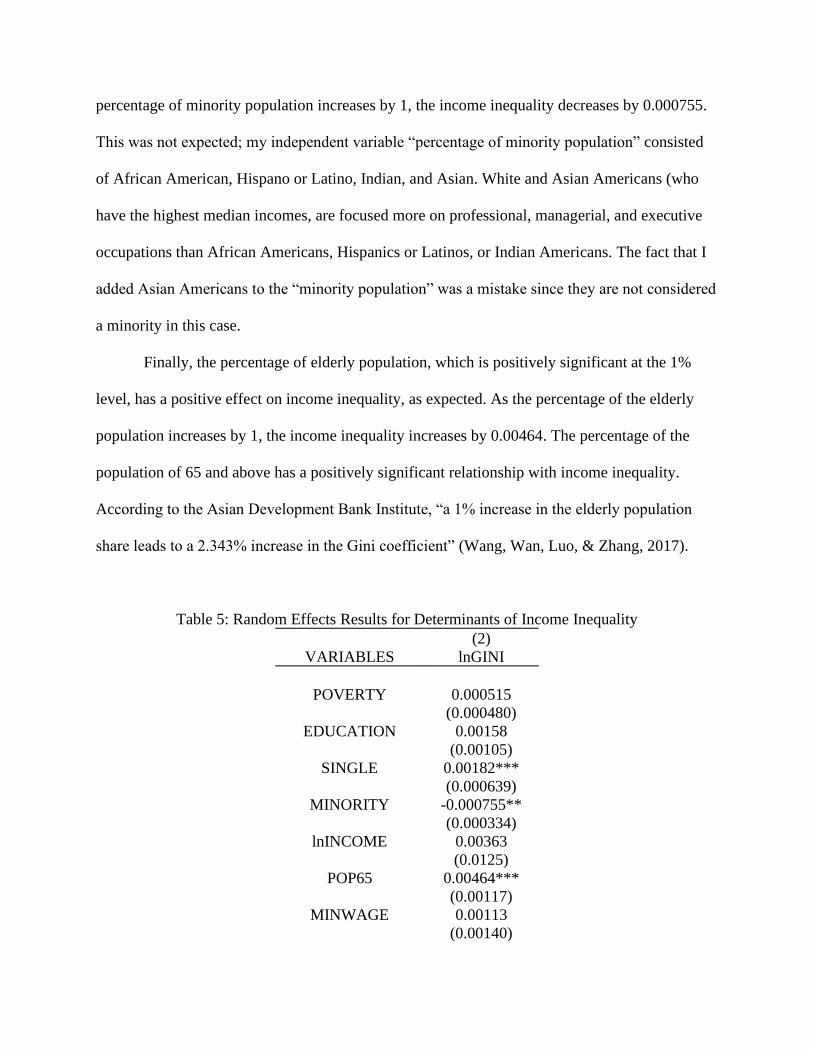
percentage of minority population increases by 1, the income inequality decreases by 0.000755.

This was not expected; my independent variable “percentage of minority population” consisted

of African American, Hispano or Latino, Indian, and Asian. White and Asian Americans (who

have the highest median incomes, are focused more on professional, managerial, and executive

occupations than African Americans, Hispanics or Latinos, or Indian Americans. The fact that I

added Asian Americans to the “minority population” was a mistake since they are not considered

a minority in this case.

Finally, the percentage of elderly population, which is positively significant at the 1%

level, has a positive effect on income inequality, as expected. As the percentage of the elderly

population increases by 1, the income inequality increases by 0.00464. The percentage of the

population of 65 and above has a positively significant relationship with income inequality.

According to the Asian Development Bank Institute, “a 1% increase in the elderly population

share leads to a 2.343% increase in the Gini coefficient” (Wang, Wan, Luo, & Zhang, 2017).

Table 5: Random Effects Results for Determinants of Income Inequality

(2)

VARIABLES lnGINI

POVERTY 0.000515

(0.000480)

EDUCATION 0.00158

(0.00105)

SINGLE 0.00182***

(0.000639)

MINORITY -0.000755**

(0.000334)

lnINCOME 0.00363

(0.0125)

POP65 0.00464***

(0.00117)

MINWAGE 0.00113

(0.00140)

DummyRecession -0.00192

(0.00366)

Constant -0.950***

(0.113)

Observations 180

Number of s_id

R2

9

0.61

Standard errors in parentheses

*** p<0.01, ** p<0.05, * p<0.1

Data availability was the major limitation for this paper. I would have liked to add other

variables like welfare, or corruption; but I was not able to find these. Gunalp, Burak. (2008),

analyzed the effects of corruption on income inequality and poverty. They defined corruption as

the number of public officials convicted in a state for crimes related to corruption. They found

robust evidence that an increase in corruption increases income inequality and poverty.

(Pettinger, 2017) ”Should the government provide more welfare support programs such as child

tax benefit and unemployment insurance in order to decrease economic inequality?” Higher

welfare programs help to decrease inequality and poverty. Higher welfare programs will give the

population with lower incomes a better life. However, there are people who argue that increasing

welfare programs may cause people to avoid work or work only a few hours (Pettinger, 2017).

6. Conclusion:

Two random effect models were applied to examine the determinants of poverty and

income inequality. Panel data for 9 southeastern states (Alabama, Arkansas, Florida, Georgia,

Louisiana, Mississippi, Oklahoma, Tennessee, South Carolina) from 2000 to 2019 were used in

this study.

The results for the determinants of poverty reveal that increases in educational

attainment, and the percentage of population over 65 years of age contributed to a decrease in

poverty (measured as the percentage of population below poverty level). On the other hand,

increases in the percentage of households led by single women contributed to an increase in

poverty. The dummy used to represent the Great Recession contributes to a positive effect on

poverty, meaning that after the Great Recession, poverty increased.

The results for the determinants of income inequality reveal that increases in the

percentage of households led by single women, and the percentage of population over 65 years

of age contributed to an increase in income inequality (measured with the Gini coefficient). On

the other hand, an increase in the percentage of minority population contributed to a decrease in

income inequality.

The way that the yearly rates of change in income inequality and poverty can happen at

the same time, brings attention to local governments and policy makers of the need to plan

policies and systems that could both lessen poverty and income inequality. By and large most

poverty decrease techniques will in general lessen income inequality somewhat, notwithstanding,

the methodologies to diminish income inequality don't really diminish poverty. For example, a

technique to decrease inequality requires interventions to advance occupation creation and

business just as to improve equity in the chance of cooperation in these positions through

improved educational levels. There is additionally a need to improve access to these new

openings by diminishing sex, pay, and racial discrimination that exist in local labor markets.

References:

(2021, April 05). Retrieved from The World Bank:

https://www.worldbank.org/en/country/georgia/overview

(2021). Retrieved from IBISWorld: https://www.ibisworld.com/united-states/economic-

profiles/georgia/#EconomicOverview

Alberto González Pandiella, M. G. (2017). Deconstructing income inequality in Costa Rica: An

income source decomposition approach. 32.

Annual percent change of the real GDP in Tennessee from 2000 to 2020. (2021). Statista.

Arkansas, D. U. (2018). Data USA. Retrieved from https://datausa.io/profile/geo/arkansas

Bleiweis, R., Boesch, D., & Gaines, A. C. (2020, August 3). The basic facts about women in

poverty. Retrieved from Center for American Progress:

https://www.americanprogress.org/issues/women/reports/2020/08/03/488536/basic-facts-

women-poverty/

Bolden, N., Clark, C., & Agbodzakey, J. (2020). Manufacturing Matters: A Case Study of

Alabama.

Bureau of Economic Analysis (U.S. Department of Commerce). (2018). Retrieved from Bureau

of Economic Analysis (U.S. Department of Commerce): https://www.bea.gov/

Bureau, C. (n.d.). United States Census Bureau. Retrieved from

https://www.census.gov/topics/income-poverty/income-inequality/about.html

Deavers, Kenneth L. and Robert A. Hoppe. “Overview of the Rural Poor in the 1980s”; pp. 3-

20. In Cynthia Duncan (ed). Rural Poverty in America. Westport CT: Auburn House,

Greenwood Publishing Group, Inc., 1992.

Department, S. R. (2021, January 20). Retrieved from Statista:

https://www.statista.com/statistics/374655/gini-index-for-income-distribution-equality-

for-us-families/

Duncan, Cynthia. “Persistent Poverty in Appalachia: Scarce Work and Rigid Stratification,”

pp.111-133. In Cynthia Duncan (ed). Rural Poverty in America. Westport CT: Auburn House,

Greenwood Publishing Group, Inc., 1992.

Economics, A. C. (n.d.). Retrieved from https://uca.edu/acre/citizens-guide-gross-domestic-

product/

Economy of Louisiana. (n.d.). Retrieved from Britannica:

https://www.britannica.com/place/Louisiana-state/The-19th-century

Economy of Louisiana. (2014). Retrieved from Britannica:

https://www.britannica.com/place/Louisiana-state/The-19th-century

Economy of Mississippi. (2020). Retrieved from Britannica:

https://www.britannica.com/place/Mississippi-state/Government-and-society

Economy of Oklahoma. (2019). Retrieved from Britannica:

https://www.britannica.com/place/Oklahoma-state/Economy

Facts about Florida. (2013). Retrieved from State of Florida:

https://www.stateofflorida.com/facts/

(2014). Florida’s Economic Future & the Impact of Aging. FLORIDA ALFA Florida Assisted

Living Federation of America.

Giovetti, O. (2020, August 27). How does education affect poverty? It can help end it. Retrieved

from Concern Worldwide US: https://www.concernusa.org/story/how-education-affects-

poverty/#:~:text=Access%20to%20high%2Dquality%20primary,to%20the%20cycle%20

of%20poverty.&text=Those%20living%20below%20the%20poverty,chance%20of%20li

ving%20in%20poverty.

Gradín, C. (2016). Why is income inequality so high in Spain?

Income Inequality in Africa. (n.d.). Retrieved from African Development Bank:

https://www.afdb.org/fileadmin/uploads/afdb/Documents/Generic-Documents/Revised-

Income%20inequality%20in%20Africa_LTS-rev.pdf

Lochner, K., Pamuk, E., P. Kennedy, B., & Kawachi, I. (2001). State-Level Income Inequality

and Individual Mortality Risk: A Prospective, Multilevel Study.

Mas, F. J. (2001). Inequality in Spain 1973-91: Contribution to a Regional Database.

McCorkell, L., & Hinkley, S. (2018, December 19). The Great Recession, Families, and the

Safety Net. Retrieved from Institute for Research on Labor and Employment:

https://irle.berkeley.edu/the-great-recession-families-and-the-safety-net/

Mississippi - State Economic Profile. (2019). Retrieved from IBISWorld:

https://www.ibisworld.com/united-states/economic-profiles/mississippi/

Muller, A. (2002). Education, income inequality, and mortality: a multiple regression analysis.

OECD. (2021). Income Inequality (indicator). doi: 10.1787/459aa7f1-en (Accessed on 24 March

2021).

Otero-Iglesias, M. (2019). Inequality in Spain: let's talk about the poor. Retrieved from Real

Instituto elcano: https://blog.realinstitutoelcano.org/en/inequality-in-spain-lets-focus-on-

the-poor/

Pettinger, T. (2017, March 19). Should welfare benefits be increased to reduce poverty?

Retrieved from Economics.help:

https://www.economicshelp.org/blog/7220/economics/should-welfare-benefits-be-

increased-to-reduce-inequality/

Priorities, C. o. (2012). Income inequality has grown in Tennessee.

Reardon, S. (2014). Retrieved from Income inequality affects our children's educational

opportunities: https://equitablegrowth.org/income-inequality-affects-our-childrens-

educational-opportunities/

Salkind, N. J. (2012, December 27). Random-Effects Models. Retrieved from

ENCYCLOPEDIA: https://methods.sagepub.com/reference/encyc-of-research-

design/n360.xml

Sermons, W., & Henry, M. (2010). Demographics of Homelessness Series: The Rising Elderly

Population.

SHADAC analysis of income inequality (gini coefficient), State Health Compare, SHADAC,

University of Minnesota, statehealthcompare.shadac.org, Accessed 24 March 2021.

(n.d.).

Social Security and Elderly Poverty. (2004, September 3). Retrieved from National Bureau of

Economic Research: https://www.nber.org/bah/2004number2/social-security-and-elderly-

poverty

Sousa-Brown, S. C. (2004). An empirical analysis of poverty adn income inequality in West

Virginia.

South Carolina. (2019). Retrieved from U.S. News: https://www.usnews.com/news/best-

states/south-carolina(2018). South Carolina Economic Analysis Report.

scworkforceinfo.com.

Statista. (2019). Percentage of households led by a single mother with children under age 18

living in the household in the U.S. in 2018, by state. Retrieved from Statista:

https://www.statista.com/statistics/242302/percentage-of-single-mother-households-in-

the-us-by-state/

Sudharshan Canagarajah, D. M. (1998). The Structure and Determinants of Inequality and

Poverty Reduction in Ghana, 1988-92.

Tennessee: Economy. (2012). Retrieved from Infoplease:

https://www.infoplease.com/encyclopedia/places/north-america/us/tennessee-state-

united-states/economy

The Progress of Education in Louisiana. (1996). Retrieved from Southwest Educational

Development Laboratory: https://sedl.org/pubs/pic01/priority.html

Unmarried Women and the Wage Gap. (2017). Retrieved from Women's Voices Women Vote:

https://www.wvwvaf.org/what-we-do/awareness/unmarried-women-wage-gap/

Wage and Hour Division. (2020). Retrieved from U.S. Department of Labor:

https://www.dol.gov/agencies/whd/mw-consolidated

Wang, C., Wan, G., Luo, Z., & Zhang, X. (2017). Aging and Inequality: The Perspective of

Labor Income Share. Asian Development Bank Institute.

William Levernier, D. S. (1995). Variation in US. State Income Inequality: 1960-1990 . 24.

Appendix A:

Table 6: Data description and sources

Variable Description Source

Gini Gini coefficient as a measure for

household income distribution

inequality, by state

Statista

Education Educational attainment, annual:

Bachelor’s degree or higher, by state

Federal Reserve Economic

Database (FRED)

Single Percentage of households led by single

mothers, by state

Statista

Minority Percentage of minority population , by

state

U.S. Census Bureau

Income Per Capita personal income, by state Federal Reserve Economic

Database (FRED)

Pop65 Percentage of population over 65 years

of age, by state

U.S. Census Bureau

MinWage Minimum wage, by state U.S. Department of Labor

Poverty Percentage of the population below

poverty level, by state

U.S. Census Bureau

DummyRecession 0 = before Great Recession;

1 = after Great Recession

Table 7: Expected signs of variables

Expected Sign

Variable lnGINI POVERTY

Dependent variables

lnGINI +

POVERTY +

Independent variables

EDUCATION - -

SINGLE + +

MINORITY + +

lnINCOME + +

POP65 + +

MINWAGE

DummyRecession

-

+

-

+

Table 8: Descriptive Statistics

Variable Mean Std. Dev. Min Max

POVERTY 15.94 2.71 10.8 23.1

EDUCATION 22.98 3.49 16.1 32.5

GINI 0.47 0.009 0.45 0.5

SINGLE 38.95 3.99 32 49

MINORITY 35.34 6.64 21.98 49

INCOME 35221 6849.29 21640 52426

POP65 14.09 2.28 9.5 20.9

MINWAGE 6.74 1.00 3.25 9.25

The following graphs represent the trends of each variable, dependent and independent

for all the states used in this paper. The states are shown with numbers in the graphs; below is

shown what state each number represents.

1. Louisiana

2. Mississippi

3. Alabama

4. Georgia

5. Florida

6. Oklahoma

7. Arkansas

8. Tennessee

9. South Carolina

Figure 4: Education (at least bachelor’s degree)(% of total population), by state

Figure 5: Gini coefficient as a measure for household income distribution inequality, by state

Figure 6: Percentage of Households Led by Single Women, by state

Figure 7: Minority Population (percentage), by state

Figure 8: Per Capita Personal Income, by state

Figure 9: Percentage of the population over 65 years old, by state

Figure 10: Percentage of the Population Below Poverty Level, by state

Figure 11: Minimum Wage, by state