Embed Size (px)
Citation preview

An Elementary Introduction to Kalman FilteringYan Pei
University of Texas at Austin
Swarnendu Biswas
University of Texas at Austin
Donald S. Fussell
University of Texas at Austin
Keshav Pingali
University of Texas at Austin
ABSTRACTKalman filtering is a classic state estimation technique used
widely in engineering applications such as statistical signal
processing and control of vehicles. It is now being used to
solve problems in computer systems, such as controlling
the voltage and frequency of processors to minimize energy
while meeting throughput requirements.
Although there are many presentations of Kalman filtering
in the literature, they are usually focused on particular prob-
lem domains such as linear systems with Gaussian noise or
robot navigation, which makes it difficult to understand the
general principles behind Kalman filtering. In this paper, we
first present the general statistical ideas behind Kalman fil-
tering at a level accessible to anyone with a basic knowledge
of probability theory and calculus, and then show how these
abstract concepts can be applied to state estimation problems
in linear systems. This separation of abstract concepts from
applications should make it easier to apply Kalman filtering
to other problems in computer systems.
KEYWORDSKalman filtering, data fusion, uncertainty, noise, state esti-
mation, covariance, BLUE estimators, linear systems
1 INTRODUCTIONKalman filtering is a state estimation technique invented in
1960 by Rudolf E. Kálmán [14]. It is used inmany areas includ-
ing spacecraft navigation, motion planning in robotics, signal
processing, and wireless sensor networks [11, 17, 21–23] be-
cause of its small computational and memory requirements,
and its ability to extract useful information from noisy data.
Recent work shows how Kalman filtering can be used in
controllers for computer systems [4, 12, 13, 19].
Although many presentations of Kalman filtering exist
in the literature [1–3, 5–10, 16, 18, 23], they are usually fo-
cused on particular applications like robot motion or state
estimation in linear systems with Gaussian noise. This can
make it difficult to see how to apply Kalman filtering to other
problems. The goal of this paper is to present the abstract
statistical ideas behind Kalman filtering independently of
particular applications, and then show how these ideas can
be applied to solve particular problems such as state estima-
tion in linear systems.
Abstractly, Kalman filtering can be viewed as an algorithm
for combining imprecise estimates of some unknown value to
obtain a more precise estimate of that value. We use informal
methods similar to Kalman filtering in everyday life. When
we want to buy a house for example, we may ask a couple of
real estate agents to give us independent estimates of what
the house is worth. For now, we use the word “independent”
informally to mean that the two agents are not allowed to
consult with each other. If the two estimates are different,
as is likely, how do we combine them into a single value to
make an offer on the house? This is an example of a datafusion problem.
One solution to our real-estate problem is to take the aver-
age of the two estimates; if these estimates are x1 and x2, theyare combined using the formula 0.5∗x1 + 0.5∗x2. This givesequal weight to the estimates. Suppose however we have ad-
ditional information about the two agents; perhaps the first
one is a novice while the second one has a lot of experience
in real estate. In that case, we may have more confidence
in the second estimate, so we may give it more weight by
using a formula such as 0.25∗x1 + 0.75∗x2. In general, we canconsider a convex combination of the two estimates, which
is a formula of the form (1−α)∗x1 + α∗x2, where 0 ≤ α ≤ 1;
intuitively, the more confidence we have in the second esti-
mate, the closer α should be to 1. In the extreme case, when
α=1, we discard the first estimate and use only the second
estimate.
The expression (1−α)∗x1 + α∗x2 is an example of a linearestimator [15]. The statistics behind Kalman filtering tell us
how to pick the optimal value of α : the weight given to an
estimate should be proportional to the confidence we have
in that estimate, which is intuitively reasonable.
To quantify these ideas, we need to formalize the concepts
of estimates and confidence in estimates. Section 2 describes
the model used in Kalman filtering. Estimates are modeled as
random samples from certain distributions, and confidence
in estimates is quantified in terms of the variances and co-variances of these distributions.
arX
iv:1
710.
0405
5v2
[cs
.SY
] 1
0 N
ov 2
017

Sections 3-5 develop the two key statistical ideas behind
Kalman filtering.
(1) How should uncertain estimates be fused optimally?
Section 3 shows how to fuse scalar estimates such
as house prices optimally. It is also shown that the
problem of fusing more than two estimates can be re-
duced to the problem of fusing two estimates at a time,
without any loss in the quality of the final estimate.
Section 4 extends these results to estimates that are vec-tors, such as state vectors representing the estimated
position and velocity of a robot or spacecraft. The
math is more complicated than in the scalar case but
the basic ideas remain the same, except that instead of
working with variances of scalar estimates, we must
work with covariance matrices of vector estimates.
(2) In some applications, estimates are vectors but only
a part of the vector may be directly observable. For
example, the state of a spacecraft may be represented
by its position and velocity, but only its position may
be directly observable. In such cases, how do we obtain
a complete estimate from a partial estimate?
Section 5 introduces the Best Linear Unbiased Estimator(BLUE), which is used in Kalman filtering for this pur-
pose. It can be seen as a generalization of the ordinary
least squares (OLS) method to problems in which data
comes from distributions rather than being a set of
discrete points.
Section 6 shows how these results can be used to solve
state estimation problems for linear systems, which is the
usual context for presenting Kalman filters. First, we con-
sider the problem of state estimation when the entire state is
observable, which can be solved using the data fusion results
from Sections 3 and 4. Then we consider the more complex
problem of state estimation when the state is only partially
observable, which requires in addition the BLUE estimator
from Section 5. Section 6.3 illustrates Kalman filtering with
a concrete example.
2 FORMALIZATION OF ESTIMATESThis section makes precise the notions of estimates and con-fidence in estimates, which were introduced informally in
Section 1.
2.1 Scalar estimatesOne way to model the behavior of an agent producing scalar
estimates such as house prices is through a probability dis-tribution function (usually shortened to distribution) like theones shown in Figure 1 in which the x-axis represents values
that can be assigned to the house, and the y-axis represents
the probability density. Each agent has its own distribution,
and obtaining an estimate from an agent corresponds to
x$500K $1 million
p1(x)
p2(x)
p(x)
Figure 1: Distributions.
drawing a random sample xi from the distribution for agent
i .Most presentations of Kalman filters assume distributions
are Gaussian but we assume that we know only the mean
µi and the variance σ 2
i of each distribution pi . We write xi :pi∼(µi ,σ 2
i ) to denote that xi is a random sample drawn from
distribution pi which has a mean of µi and a variance of σ 2
i .
The reciprocal of the variance of a distribution is sometimes
called the precision of that distribution.
The informal notion of “confidence in the estimates made
by an agent” is quantified by the variance of the distribution
from which the estimates are drawn. An experienced agent
making high-confidence estimates is modeled by a distri-
bution with a smaller variance than one used to model an
inexperienced agent; notice that in Figure 1, the inexperi-
enced agent is “all over the map.”
This approach to modeling confidence in estimates may
seem nonintuitive since there is no mention of how close
the estimates made by an agent are to the actual value of the
house. In particular, an agent can make estimates that are
very far off from the actual value of the house but as long as
his estimates fall within a narrow range of values, we would
still say that we have high confidence in his estimates. In
statistics, this is explained by making a distinction between
accuracy and precision. Accuracy is a measure of how close
an estimate of a quantity is to the true value of that quan-
tity (the true value is sometimes called the ground truth).Precision on the other hand is a measure of how close the
estimates are to each other, and is defined without reference
to ground truth. A metaphor that is often used to explain
this difference is shooting at a bullseye. In this case, ground
truth is provided by the center of the bullseye. A precise
shooter is one whose shots are clustered closely together
even if they may be far from the bullseye. In contrast, the
shots of an accurate but not precise shooter would be scat-
tered widely in a region surrounding the bullseye. For the
problems considered in this paper, there may be no ground
truth, and confidence in estimates is related to precision, not
accuracy.
The informal notion of getting independent estimates from
the two agents is modeled by requiring that estimates x1 and
2
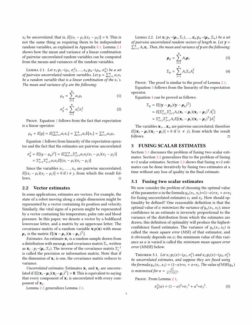
x2 be uncorrelated; that is, E[(x1 − µ1)(x2 − µ2)] = 0. This is
not the same thing as requiring them to be independent
random variables, as explained in Appendix 8.1. Lemma 2.1
shows how the mean and variance of a linear combination
of pairwise uncorrelated random variables can be computed
from the means and variances of the random variables.
Lemma 2.1. Let x1:p1∼(µ1,σ 2
1), ...,xn :pn∼(µn ,σ 2
n) be a setof pairwise uncorrelated random variables. Let y =
∑ni=1 αixi
be a random variable that is a linear combination of the xi ’s.The mean and variance of y are the following:
µy =n∑i=1
αiµi (1)
σ 2
y =
n∑i=1
α2
i σ2
i (2)
Proof. Equation 1 follows from the fact that expectation
is a linear operator:
µy = E[y] = E[∑ni=1αixi ] =
∑ni=1αiE[xi ] =
∑ni=1αiµi .
Equation 2 follows from linearity of the expectation opera-
tor and the fact that the estimates are pairwise uncorrelated:
σ 2
y = E[(y − µy )2] = E[∑ni=1Σ
nj=1αiα j (xi − µi )(x j − µ j )]
= Σni=1Σnj=1αiα jE[(xi − µi )(x j − µ j )]
Since the variables x1, . . . ,xn are pairwise uncorrelated,
E[(xi − µi )(x j − µ j )] = 0 if i , j, from which the result fol-
lows. □
2.2 Vector estimatesIn some applications, estimates are vectors. For example, the
state of a robot moving along a single dimension might be
represented by a vector containing its position and velocity.
Similarly, the vital signs of a person might be represented
by a vector containing his temperature, pulse rate and blood
pressure. In this paper, we denote a vector by a boldfaced
lowercase letter, and a matrix by an uppercase letter. The
covariance matrix of a random variable x:p(x) with mean
µµµx is the matrix E[(x − µµµx )(x − µµµx )T].Estimates: An estimate xi is a random sample drawn from
a distributionwithmean µµµi and covariancematrix Σi , writtenas xi : pi∼(µµµi , Σi ). The inverse of the covariance matrix Σ−1
iis called the precision or information matrix. Note that if
the dimension of xi is one, the covariance matrix reduces to
variance.
Uncorrelated estimates: Estimates xi and xj are uncorre-
lated if E[(xi −µµµi )(xj −µµµ j )T] = 000. This is equivalent to sayingthat every component of xi is uncorrelated with every com-
ponent of xj .
Lemma 2.2 generalizes Lemma 2.1.
Lemma 2.2. Let x1:p1∼(µµµ1, Σ1), ...,xn :pn∼(µµµn , Σn) be a setof pairwise uncorrelated random vectors of lengthm. Let y =∑n
i=1Aixi . Then, themean and variance of y are the following:
µµµy =n∑i=1
Aiµµµi (3)
Σy =n∑i=1
AiΣiAT
i (4)
Proof. The proof is similar to the proof of Lemma 2.1.
Equation 3 follows from the linearity of the expectation
operator.
Equation 4 can be proved as follows:
Σy = E[(y − µµµy )(y − µµµy )T]= E[Σni=1Σ
nj=1Ai (xi − µµµi )(xj − µµµ j )TAT
j ]= Σni=1Σ
nj=1AiE[(xi − µµµi )(xj − µµµ j )T]AT
j
The variables x1, ..xn are pairwise uncorrelated, therefore
E[(xi − µµµi )(xj − µµµ j )] = 0 if (i , j), from which the result
follows. □
3 FUSING SCALAR ESTIMATESSection 3.1 discusses the problem of fusing two scalar esti-
mates. Section 3.2 generalizes this to the problem of fusing
n>2 scalar estimates. Section 3.3 shows that fusing n>2 esti-mates can be done iteratively by fusing two estimates at a
time without any loss of quality in the final estimate.
3.1 Fusing two scalar estimatesWe now consider the problem of choosing the optimal value
of the parameterα in the formulayα (x1,x2)=(1−α)∗x1 + α∗x2for fusing uncorrelated estimates x1 and x2. How should op-
timality be defined? One reasonable definition is that the
optimal value of α minimizes the variance ofyα (x1,x2); sinceconfidence in an estimate is inversely proportional to the
variance of the distribution from which the estimates are
drawn, this definition of optimality will produce the highest-
confidence fused estimates. The variance of yα (x1,x2) iscalled the mean square error (MSE) of that estimator, and
it obviously depends on α ; the minimum value of this vari-
ance as α is varied is called the minimum mean square errorerror (MMSE) below.
Theorem 3.1. Let x1:p1(x)∼(µ1,σ 2
1) and x2:p2(x)∼(µ2,σ 2
2)
be uncorrelated estimates, and suppose they are fused usingthe formulayα (x1,x2) = (1−α)∗x1 + α∗x2. The value ofMSE(yα )is minimized for α = σ 2
1
σ 1
2+σ 2
2.
Proof. From Lemma 2.1,
σ 2
y (α) = (1 − α)2∗σ 1
2 + α2∗σ 2
2. (5)
3

Differentiating σ 2
y (α)with respect to α and setting the deriva-
tive to zero proves the result. The second derivative, (σ 2
1+σ 2
2),
is positive, showing that σ 2
y (α) reaches a minimum at this
point.
In the literature, this optimal value of α is called the
Kalman gain K . □
Substituting K into the linear fusion model, we get the
optimal linear estimator y(x1,x2):
y(x1,x2) =σ 2
2
σ 1
2 + σ 2
2∗x1 +
σ 2
1
σ 1
2 + σ 2
2∗x2
As a step towards fusion of n>2 estimates, it is useful to
rewrite this as follows:
y(x1,x2) =1
σ 2
1
1
σ 1
2+ 1
σ 2
2
∗x1 +1
σ 2
2
1
σ 1
2+ 1
σ 2
2
∗x2 (6)
Substituting K into Equation 5 gives the following expres-
sion for the variance of y:
σ 2
y =1
1
σ 1
2+ 1
σ 2
2
(7)
The expressions for y and σy are complicated because they
contain the reciprocals of variances. If we let ν1 and ν2 denotethe precisions of the two distributions, the expressions for yand νy can be written more simply as follows:
y(x1,x2) =ν1
ν1 + ν2∗x1 +
ν2ν1 + ν2
∗x2 (8)
νy = ν1 + ν2 (9)
These results say that the weight we should give to an
estimate is proportional to the confidence we have in that
estimate, which is intuitively reasonable. Note that if µ1=µ2,the expectation E[yα ] is µ1(=µ2) regardless of the value α .In this case, yα is said to be an unbiased estimator, and the
optimal value of α minimizes the variance of the unbiased
estimator.
3.2 Fusing multiple scalar estimatesThe approach in Section 3.1 can be generalized to optimally
fuse multiple pairwise uncorrelated estimates x1,x2, ...,xn .Let yα (x1, ..,xn) denote the linear estimator given parame-
ters α1, ..,αn , which we denote by α .
Theorem 3.2. Let pairwise uncorrelated estimatesxi (1≤i≤n)drawn from distributionspi (x)∼(µi ,σ 2
i ) be fused using the lin-ear model yα (x1, ..,xn) =
∑ni=1 αixi where
∑ni=1 αi = 1. The
value of MSE(yα ) is minimized for
αi =
1
σ 2
i∑ni=1
1
σ 2
i
.
Proof. From Lemma 2.1, σ 2
y (α) =∑n
i=1 αi2σ i
2. To find the
values of αi that minimize the variance σ 2
y under the con-
straint that the αi ’s sum to 1, we use the method of Lagrange
multipliers. Define
f (α1, ...,αn) =n∑i=1
αi2σ i
2 + λ(n∑i=1
αi − 1)
where λ is the Lagrange multiplier. Taking the partial deriva-
tives of f with respect to eachαi and setting these derivativesto zero, we find α1σ
2
1= α2σ
2
2= ... = αnσ
2
n = −λ/2. From this,
and the fact that sum of the αi ’s is 1, the result follows. □
The variance is given by the following expression:
σ 2
y =1
n∑i=1
1
σ 2
i
. (10)
As in Section 3.1, these expressions are more intuitive if
the variance is replaced with precision.
y(x1, ..,xn) =n∑i=1
νiν1+...+νn
∗ xi (11)
νy =n∑i=1
νi (12)
Equations 11 and 12 generalize Equations 8 and 9.
3.3 Incremental fusing is optimalIn many applications, the estimates x1,x2, ...,xn become
available successively over a period of time. While it is
possible to store all the estimates and use Equations 11
and 12 to fuse all the estimates from scratch whenever a
new estimate becomes available, it is possible to save both
time and storage if one can do this fusion incrementally.
In this section, we show that just as a sequence of num-
bers can be added by keeping a running sum and adding
the numbers to this running sum one at a time, a sequence
of n>2 estimates can be fused by keeping a “running es-
timate” and fusing estimates from the sequence one at a
time into this running estimate without any loss in the
quality of the final estimate. In short, we want to show
that y(x1,x2, ...,xn) = y(y(y(x1,x2),x3)...,xn). Note that thisis not the same thing as showing y, interpreted as a binary
function, is associative.
Figure 2 shows the process of incrementally fusing es-
timates. Imagine that time progresses from left to right in
this picture. Estimate x1 is available initially, and the other
estimates xi become available in succession; the precision of
each estimate is shown in parentheses next to each estimate.
When the estimate x2 becomes available, it is fused with x1using Equation 8. In Figure 2, the labels on the edges con-
necting x1 and x2 to y(x1,x2) are the weights given to these
4

+(ν1)x1
ν1
ν1+ν
2
x2(ν2)
ν2
ν1+ν
2
y(x1, x2)(ν1 + ν2)
+
x3(ν3)
ν1+ν
2
ν1+ν
2+ν
3
ν3
ν1+ν
2+ν
3
. . .
y((x1, x2), x3)(ν1 + ν2 + ν3)
+
xn−1(νn−1)
νn−1ν1+···+νn−1
y(x1, . . ., xn−1)(ν1 + · · · + νn−1)
+
xn(νn )
νnν1+···+νn
ν1+···+νn−1ν1+···+νn
y(x1, . . ., xn )(ν1 + · · · + νn )
Figure 2: Dataflow graph for incremental fusion.
estimates in Equation 8. When estimate x3 becomes available,
it is fused with y(x1,x2) using Equation 8; as before, the la-
bels on the edges correspond to the weights given to y(x1,x2)and x3 when they are fused to produce y(y(x1,x2),x3).
The contribution ofxi to the final value y(y(y(x0,x1),x2)...,xn)is given by the product of the weights on the path from xi tothe final value in Figure 2. As shown below, this product has
the same value as the weight of xi in Equation 11, showing
that incremental fusion is optimal.
νiν1 + ... + νi
∗ ν1 + ... + νiν1 + ... + νi+1
∗ ... ∗ ν1 + ... + νn−1ν1 + ... + νn
=νi
ν1 + ... + νn
3.4 SummaryThe main result in this section can be summarized infor-
mally as follows.When using a linear model to fuse uncertainscalar estimates, the weight given to each estimate should beinversely proportional to the variance of that estimate. Fur-thermore, when fusing n>2 estimates, estimates can be fusedincrementally without any loss in the quality of the final re-sult.More formally, the results in this section for fusing scalar
estimates are often expressed in terms of the Kalman gain,
as shown below; these equations can be applied recursively
to fuse multiple estimates.
x1 : p1∼(µ1,σ 2
1), x2 : p2∼(µ2,σ 2
2)
K =σ 2
1
σ 2
1+ σ 2
2
=ν2
ν1 + ν2(13)
y(x1,x2) = x1 + K(x2 − x1) (14)
µy = µ1 + K(µ2 − µ1) (15)
σ 2
y = σ 1
2 − Kσ 1
2 or νy = ν1 + ν2 (16)
4 FUSING VECTOR ESTIMATESThis section addresses the problem of fusing estimates when
the estimates are vectors. Although the math is more com-
plicated, the conclusion is that the results in Section 3 for
fusing scalar estimates can be extended to the vector case
simply by replacing variances with covariance matrices, asshown in this section.
4.1 Fusing multiple vector estimatesFor vectors, the linear data fusion model is
yA(x1,x2, ..,xn) =n∑i=1
Aixi where
n∑i=1
Ai = I . (17)
Here A stands for the matrix parameters (A1, ...,An). All thevectors are assumed to be of the same length. If the means µµµiof the random variables xi are identical, this is an unbiased
estimator.
Optimality: The MSE in this case is the expected value of
the two-norm of (yA−µµµyA ), which is E[(yA−µµµyA )T(yA−µµµyA )].Note that if the vectors have length 1, this reduces to variance.
The parametersA1, ...,An in the linear data fusion model are
chosen to minimize this MSE.Theorem 4.1 generalizes Theorem 3.2 to the vector case.
The proof of this theorem uses matrix derivatives and is
given in Appendix 8.3 since it is not needed for understand-
ing the rest of this paper. What is important is to compare
Theorems 4.1 and 3.2 and notice that the expressions are
similar, the main difference being that the role of variance
in the scalar case is played by the covariance matrix in the
vector case.
Theorem 4.1. Let pairwise uncorrelated estimatesxi (1≤i≤n)drawn from distributionspi (x)=(µµµi , Σi ) be fused using the lin-ear model yA(x1, ..,xn) =
∑ni=1Aixi , where
∑ni=1Ai = I . The
MSE(yA) is minimized for
Ai = (n∑j=1
Σ−1j )−1Σ−1
i . (18)
The covariance matrix of the optimal estimator y can be
determined by substituting the optimal Ai values into the
expression for Σy in Lemma 2.2.
Σy = (n∑j=1
Σ−1j )−1 (19)
In the vector case, precision is the inverse of a covariance
matrix, denoted by N . Equations 20–21 use precision to ex-
press the optimal estimator and its variance, and generalize
Equations 11–12 to the vector case.
y(x1, ...,xn) =n∑i=1
( n∑j=1
Nj)−1
Nixi (20)
Ny =
n∑j=1
Nj (21)
As in the scalar case, fusion of n>2 vector estimates can
be done incrementally without loss of precision. The proof
is similar to the one in Section 3.3, and is omitted.
There are several equivalent expressions for the Kalman
gain for the fusion of two estimates. The following one,
5

which is easily derived from Equation 18, is the vector analog
of Equation 13:
K = Σ1(Σ1 + Σ2)−1 (22)
The covariance matrix of y can be written as follows.
Σy = Σ1(Σ1 + Σ2)−1Σ2 (23)
= KΣ2 = Σ1 − KΣ1 (24)
4.2 SummaryThe results in this section can be summarized in terms of the
Kalman gain K as follows:
x1 : p1∼(µµµ1, Σ1), x2 : p2∼(µµµ2, Σ2)
K = Σ1(Σ1 + Σ2)−1 = (N1 + N2)−1N2 (25)
y(x1,x2) = x1 + K(x2 − x1) (26)
µµµy = µµµ1 + K(µµµ2 − µµµ1) (27)
Σy = Σ1 − KΣ1 or Ny = N1 + N2 (28)
5 BEST LINEAR UNBIASED ESTIMATOR(BLUE)
In some applications, estimates are vectors but only part of
the vector may be given to us directly, and it is necessary
to estimate the hidden portion. This section introduces a
statistical method called the Best Linear Unbiased Estimator(BLUE).
x
y
x1
y1
(µxµy
)(y − µy) = ΣyxΣ
−1xx(x − µx)
Figure 3: BLUE line corresponding to Equation 29
Consider the general problem of determining a value for
vector y given a value for a vector x. If there is a functionalrelationship between x and y (say y=F (x) and F is given),
it is easy to compute y given a value for x. In our context
however, x and y are random variables so such a precise
functional relationship will not hold. The best we can do is
to estimate the likely value of y, given a value of x and the
information we have about how x and y are correlated.
Figure 3 shows an example in which x and y are scalar-
valued random variables. The grey ellipse in this figure, called
a confidence ellipse, is a projection of the joint distribution of
x and y onto the (x ,y) plane that shows where some large
proportion of the (x ,y) values are likely to be. For a given
value x1, there are in general many points (x1,y) that liewithin this ellipse, but these y values are clustered around
the line shown in the figure so the value y1 is a reasonableestimate for the value of y corresponding to x1. This line,called the best linear unbiased estimator (BLUE), is the analogof ordinary least squares (OLS) for distributions. Given a set
of discrete points (xi ,yi ) where each xi and yi are scalars,OLS determines the “best” linear relationship between these
points, where best is defined as minimizing the square error
between the predicted and actual values of yi . This relationcan then be used to predict a value for y given a value for
x . The BLUE estimator presented below generalizes this to
the case when x and y are vectors, and are random variables
obtained from distributions instead of a set of discrete points.
5.1 Computing BLUELet x:px∼(µx, Σxx) and y:py∼(µy, Σyy) be random variables.
Consider a linear estimator yA,b(x)=Ax+b. How should we
chooseA and b? As in the OLS approach, we can pick values
that minimize the MSE between random variable y and the
estimate y.
MSEA,b(y) = E[(y − y)T(y − y)]= E[(y − (Ax + b))T(y − (Ax + b))]= E[yTy − 2yT(Ax + b) + (Ax + b)T(Ax + b)]
Setting the partial derivatives ofMSEA,b(y)with respect tob andA to zero, we find that b = (µy−Aµx), andA = ΣyxΣ
−1xx ,
where Σyx is the covariance between y and x. Therefore, thebest linear estimator is
y = µy + ΣyxΣ−1xx(x − µx) (29)
This is an unbiased estimator because the mean of y is
equal to µy. Note that if Σyx = 0 (that is, x and y are uncorre-
lated), the best estimate of y is just µy, so knowing the valueof x does not give us any additional information about y as
one would expect. In Figure 3, this corresponds to the case
when the BLUE line is parallel to the x-axis. At the other
extreme, suppose that y and x are functionally related so
y = Cx. In that case, it is easy to see that Σyx = CΣxx, so
y = Cx as expected. In Figure 3, this corresponds to the case
when the confidence ellipse shrinks down to the BLUE line.
The covariance matrix of this estimator is the following:
Σy = Σyy − ΣyxΣ−1xxΣxy (30)
6

Intuitively, knowing the value of x permits us to reduce
the uncertainty in the value of y by an additive term that
depends on how strongly y and x are correlated.
It is easy to show that Equation 29 is a generalization of
ordinary least squares in the sense that if we compute means
and variances of a set of discrete data (xi ,yi ) and substitute
into Equation 29, we get the same line that is obtained by
using OLS.
6 KALMAN FILTERS FOR LINEARSYSTEMS
In this section, we apply the algorithms developed in Sec-
tions 3-5 to the particular problem of estimating the state of
linear systems, which is the classical application of Kalman
filtering.
Figure 4(a) shows how the evolution over time of the state
of such a system can be computed if the initial state x0
and the model of the system dynamics are known precisely.
Time advances in discrete steps. The state of the system
at any time step is a function of the state of the system at
the previous time step and the control inputs applied to the
system during that interval. This is usually expressed by
an equation of the form xt+1 = ft (xt ,ut ) where ut is the
control input. The function ft is nonlinear in the general case,and can be different for different steps. If the system is linear,
the relation for state evolution over time can be written as
xt+1 = Ftxt + Btut , where Ft and Bt are (time-dependent)
matrices that can be determined from the physics of the
system. Therefore, if the initial state x0 is known exactly
and the system dynamics are modeled perfectly by the Ftand Bt matrices, the evolution of the state with time can be
computed precisely.
In general however, we may not know the initial state
exactly, and the system dynamics and control inputs may
not be known precisely. These inaccuracies may cause the
computed and actual states to diverge unacceptably over
time. To avoid this, we can make measurements of the state
after each time step. If these measurements were exact and
the entire state could be observed after each time step, there
would of course be no need to model the system dynamics.
However, in general, (i) the measurements themselves are
imprecise, and (ii) some components of the state may not be
directly observable by measurements.
6.1 Fusing complete observations of thestate
If the entire state can be observed through measurements,
we have two imprecise estimates for the state after each
time step, one from the model of the system dynamics and
one from the measurement. If these estimates are uncorre-
lated and their covariance matrices are known, we can use
Equations 25:28 to fuse these estimates and compute the
covariance matrix of this fused estimate. The fused estimate
of the state is fed into the model of the system to compute
the estimate of the state and its covariance at the next time
step, and the entire process is repeated.
Figure 4(b) shows the dataflow diagram of this compu-
tation. For each state xt+1 in the precise computation of
Figure 4(a), there are three random variables in Figure 4(b):
the estimate from the model of the dynamical system, de-
noted by xt+1 |t , the estimate from the measurement, denoted
by zt+1, and the fused estimate, denoted by xt+1 |t+1. Intu-itively, the notation xt+1 |t stands for the estimate of the state
at time (t+1) given the information at time t , and it is often
referred to as the a priori estimate. Similarly, xt+1 |t+1 is thecorresponding estimate given the information available attime (t+1), which includes information from the measure-
ment, and is often referred to as the a posteriori estimate. To
set up this computation, we introduce the following notation.
• The initial state is denoted by x0 and its covariance by
Σ0 |0.
• Uncertainty in the system model and control inputs is
represented by making xt+1 |t a random variable and
introducing a zero-mean noise termwt into the state
evolution equation, which becomes
xt+1 |t = Ftxt |t + Btut +wt (31)
The covariance matrix ofwt is denoted by Qt andwtis assumed to be uncorrelated with xt |t .
• The imprecise measurement at time t+1 is modeled by
a random variable zt+1 = xt+1 + vt+1 where vt+1 is anoise term. vt+1 has a covariance matrix Rt+1 and is
uncorrelated to xt+1 |t .Examining Figure 4(c), we see that if we can compute
Σt+1 |t , the covariance matrix of xt+1 |t , from Σt |t , we haveeverything we need to implement the vector data fusion
technique described in Section 4. This can be done by apply-
ing Equation 4, which tells us that Σt+1 |t = FtΣt |t FT
t +Qt .
This equation propagates uncertainty in the input of ft toits output.
Figure 4(c) puts all the pieces together. Although the com-
putations appear to be complicated, the key thing to note is
that they are a direct application of the vector data fusion
technique of Section 4 to the special case of linear systems.
6.2 Fusing partial observations of the stateIf some components of the state cannot be measured directly,
the prediction phase remains unchanged from Section 6.1 but
the fusion phase is different and can be understood intuitively
in terms of the following steps.
(i) The portion of the a priori state estimate corresponding
to the observable part is fused with the measurement,
7

x0 x1f0 ..... xt xt+1ft
(a) Discrete-time dynamical system.
+ ..... +x0 |0
(Σ0 |0)
f0x1 |0
(Σ1 |0)
z1(R1)
x1 |1
(Σ1 |1)
xt |t(Σt |t )
ftxt+1 |t(Σt+1 |t )
zt+1(Rt+1)
xt+1 |t+1(Σt+1 |t+1)
(b) Dynamical system with uncertainty.
(Σ0 |0)x0 xt+1 |t = Ftxt |t + Btut
Σt+1 |t = FtΣt |tFTt + Qt
(Σt+1 |t )xt+1 |t
Kt+1 = Σt+1 |t (Σt+1 |t + Rt+1)−1
xt+1 |t+1 = xt+1 |t + Kt+1(zt+1 - xt+1 |t )Σt+1 |t+1 = (I - Kt+1)Σt+1 |t
zt+1(Rt+1)
(Σt+1 |t+1)xt+1 |t+1
Predictor Measurement Fusion+
(c) Implementation of the dataflow diagram (b).
(Σ0 |0)x0 xt+1 |t = Ftxt |t + Btut
Σt+1 |t = FtΣt |tFTt + Qt
(Σt+1 |t )xt+1 |t
Kt+1 = Σt+1 |tHT(HΣt+1 |tH
T+ Rt+1)
−1
xt+1 |t+1 = xt+1 |t + Kt+1(zt+1 - Hxt+1 |t )Σt+1 |t+1 = (I - Kt+1H)Σt+1 |t
zt+1(Rt+1)
(Σt+1 |t+1)xt+1 |t+1
Predictor Measurement Fusion+
(d) Implementation of the dataflow diagram (b) for systems with partial observability.
Figure 4: State estimation using Kalman filtering
using the techniques developed in Sections 3-4. The
result is the a posteriori estimate of the observable state.(ii) The BLUE estimator in Section 5 is used to obtain the a
posteriori estimate of the hidden state from the a poste-riori estimate of the observable state.
(iii) The a posteriori estimates of the observable and hidden
portions of the state are composed to produce the aposteriori estimate of the entire state.
The actual implementation produces the final result di-
rectly without going through these steps, as shown in Fig-
ure 4(d) but these incremental steps are useful for under-
standing how all this works.
6.2.1 Example: 2D state. Figure 5 illustrates these stepsfor a two-dimensional problem in which the state-vector
has two components, and only the first component can be
measured directly. We use the simplified notation below to
focus on the essentials.
• a priori state estimate: xi =(hici
)• covariancematrix of a priori estimate: Σi =
(σ 2
h σhcσch σ 2
c
)• a posteriori state estimate: xo =
(hoco
)• measurement: z
• variance of measurement: r 2
The three steps discussed above for obtaining the a pos-teriori estimate involve the following calculations, shown
pictorially in Figure 5.
(i) The a priori estimate of the observable state is hi . Thea posteriori estimate is obtained from Equation 14.
8

ho = hi +σ 2
h(σ 2
h+r2) (z − hi ) = hi + Kh(z − hi )
(ii) The a priori estimate of the hidden state is ci . The aposteriori estimate is obtained from Equation 29.
co = ci +σhc
σ 2
h
∗σ 2
h
(σ 2
h + r2)(z − hi ) = ci +
σhc
(σ 2
h + r2)(z − hi )
= ci + Kc (z − hi )
(iii) Putting these together, we get(hoco
)=
(hici
)+
(KhKc
)(z − hi )
As a step towards generalizing this result in Section 6.2.2,
it is useful to rewrite this expression using matrices. Define
H =(1 0
)andR =
(r 2). Then xo = xi + K(z − Hxi )where
K = Σi ∗ HT(HΣiHT + R)−1.
h
c
h0
c0
Σi
Σo
( )
z
(hici
)(hoco
)
Kh(z − hi )
Kc (z − hi )r 2
Figure 5: Computing the a posteriori estimate whenpart of the state is not observable
6.2.2 General case. In general, suppose that the observ-
able portion of a state estimate x is given by Hx where His a full row-rank matrix. Let C be a basis for the orthogo-
nal complement of H (in the 2D example in Section 6.2.1,
H = (1 0) and C = (0 1)). The covariance between Cx and
Hx is easily shown to be CΣHTwhere Σ is the covariance
matrix of x. The three steps for computing the a posterioriestimate from the a priori estimate in the general case are
the following.
(i) The a priori estimate of the observable state is Hxt+1 |t .The a posteriori estimate is obtained from Equation 26:
Hxt+1 |t+1 = Hxt+1 |t+HΣt+1 |tHT(HΣt+1 |tH
T+Rt+1)−1(zt+1−Hxt+1 |t )
Let Kt+1=Σt+1 |tHT(HΣt+1 |tH
T+Rt+1)−1. The a posteri-ori estimate of the observable state can be written in
terms of Kt+1 as follows:
Hxt+1 |t+1 = Hxt+1 |t+HKt+1(zt+1−Hxt+1 |t ) (32)
(ii) The a priori estimate of the hidden state isCxt+1 |t . Thea posteriori estimate is obtained from Equation 29:
Cxt+1 |t+1=Cxt+1 |t+(CΣt+1 |tHT)(HΣt+1 |tHT)−1HKt+1(zt+1−Hxt+1 |t )
=Cxt+1 |t +CKt+1(zt+1 − Hxt+1 |t ) (33)
(iii) Putting the a posteriori estimates (32) and (33) together,(HC
)xt+1 |t+1 =
(HC
)xt+1 |t +
(HC
)Kt+1(zt+1 − Hxt+1 |t )
Since
(HC
)is invertible, it can be canceled from the left
and right hand sides, giving the equation
xt+1 |t+1 = xt+1 |t + Kt+1(zt+1 − Hxt+1 |t ) (34)
To compute Σt+1 |t+1, the covariance of xt+1 |t+1, note thatxt+1 |t+1 = (I − Kt+1H )xt+1 |t + Kt+1zt+1. Sincext+1 |t and zt+1are uncorrelated, it follows from Lemma 2.2 that
Σt+1 |t+1 = (I − Kt+1H )Σt+1 |t (I − Kt+1H )T + Kt+1Rt+1KTt+1
Substituting the value of Kt+1 and simplifying, we get
Σt+1 |t+1 = (I − Kt+1H )Σt+1 |t (35)
Figure 4(d) puts all this together. Note that if the entire
state is observable,H = I and the computations in Figure 4(d)
reduce to those of Figure 4(c) as expected.
6.3 An exampleTo illustrate the concepts discussed in this section, we use a
simple example in which a car starts from the origin at time
t=0 and moves right along the x-axis with an initial speed
of 100 m/sec. and a constant deceleration of 5m/sec .2 untilit comes to rest.
The state-vector of the car has two components, one for
the distance from the origin d(t) and one for the speed v(t).If time is discretized in steps of 0.25 seconds, the difference
equation for the dynamics of the system is easily shown to
be the following:(dn+1vn+1
)=
(1 0.250 1
) (dnvn
)+
(0 0.031250 0.25
) (0
−5
)(36)
where
(d0v0
)=
(0
100
).
The gray lines in Figure 6 show the evolution of velocity
and position with time according to this model. Because of
uncertainty in modeling the system dynamics, the actual
evolution of the velocity and position will be different in
practice. The red lines in Figure 6 shows one trajectory for
this evolution, corresponding to a Gaussian noise term with
covariance
(4 2
2 4
)in Equation 31 (because this noise term
is random, there are many trajectories for the evolution, and
9

0 2 4 6 8 10 12 14 16 18 20
t
-20
0
20
40
60
80
100
120
Ve
locity
Velocity
MeasuredModel-onlyGround TruthEstimated
0 2 4 6 8 10 12 14 16 18 20
t
0
200
400
600
800
1000
1200
Dis
tan
ce
Distance
Ground TruthEstimatedModel-only
Figure 6: Estimates of the car’s state over time
we are just showing one of them). The red lines correspond
to “ground truth” in our experiments.
Suppose that only the velocity is directly observable. The
green points in Figure 6 show the noisy measurements at
different time-steps, assuming the noise is modeled by a
Gaussian with variance 8. The blue lines show the a posterioriestimates of the velocity and position. It can be seen that the
a posteriori estimates track the ground truth quite well even
when the ideal system model (the grey lines) is inaccurate
and the measurements are noisy.
6.4 DiscussionEquation 34 shows that the a posteriori state estimate is a
linear combination of the a priori state estimate (xt+1 |t ) andthe estimate of the observable state from the measurement
(zt+1). Note however that unlike in Sections 3 and 4, the
Kalman gain is not a dimensionless value if the entire state
is not observable.
Although the optimality results of Sections 3-5 were used
in the derivation of this equation, it does not follow that
Equation 34 is the optimal unbiased linear estimator for com-
bining these two estimates. However, this is easy to show
using theMSE minimization technique that we have used re-
peatedly in this paper; assume that the a posteriori estimator
is of the formK1xt+1 |t+K2zt+1, and find the values ofK1 and
K2 that produce an unbiased estimator with minimum MSE.In fact, this is the point of departure for standard presen-
tations of this material. The advantage of the presentation
given here is that it exposes the general statistical concepts
that underlie Kalman filtering.
Most presentations in the literature also begin by assuming
that the noise termswt in the state evolution equation and vtin the measurement are Gaussian. Some presentations [1, 9]
use properties of Gaussians to derive the results in Sections 3
although as we have seen, these results do not depend on
distributions being Gaussians.
Gaussians however enter the picture in a deeper way if
one considers nonlinear estimators. It can be shown that if
the noise terms are not Gaussian, there may be nonlinear
estimators whoseMSE is lower than that of the linear estima-
tor presented in Figure 4(d) but that if the noise is Gaussian,
the linear estimator is as good as any unbiased nonlinear
estimator (that is, the linear estimator is aminimum varianceunbiased estimator (MVUE)). This result is proved using the
Cramer-Rao lower bound [20]. The presentation in this paper
is predicated on the belief that this property is not needed
to understand what Kalman filtering does.
7 CONCLUSIONSKalman filtering is a classic state estimation technique used
widely in engineering applications. Although there are many
presentations of this technique in the literature, most of
them are focused on particular applications like robot mo-
tion, which can make it difficult to understand how to apply
Kalman filtering to other problems. In this paper, we have
shown that two statistical ideas - fusion of uncertain esti-
mates and unbiased linear estimators for correlated variables
- provide the conceptual underpinnings for Kalman filtering.
By combining these ideas, standard results on Kalman fil-
tering in linear systems can be derived in an intuitive and
straightforward way that is simpler than other presentations
of this material in the literature.
We believe the approach presented in this paper makes it
easier to understand the concepts that underlie Kalman fil-
tering and to apply it to new problems in computer systems.
ACKNOWLEDGMENTSThis research was supported by NSF grants 1337281, 1406355,
and 1618425, and by DARPA contracts FA8750-16-2-0004
and FA8650-15-C-7563. The authors would like to thank Ivo
Babuska (UT Austin), Gianfranco Bilardi (Padova), Augusto
Ferrante (Padova), Jayadev Misra (UT Austin), Scott Niekum
10

(UT Austin), Charlie van Loan (Cornell), Etienne Vouga (UT
Austin) and Peter Stone (UT Austin) for their feedback on
this paper.
REFERENCES[1] Tim Babb. 2015. How a Kalman filter works, in pictures.
http://www.bzarg.com/p/how-a-kalman-filter-works-in-pictures/.
(2015).
[2] A. V. Balakrishnan. 1987. Kalman Filtering Theory. Optimization
Software, Inc., Los Angeles, CA, USA.
[3] Allen L. Barker, Donald E. Brown, and Worthy N. Martin. 1994.
Bayesian Estimation and the Kalman Filter. Technical Report. Char-lottesville, VA, USA.
[4] K. Bergman. 2009. Nanophotonic Interconnection Networks in Multi-
core Embedded Computing. In 2009 IEEE/LEOSWinter Topicals MeetingSeries. 6–7. https://doi.org/10.1109/LEOSWT.2009.4771628
[5] Liyu Cao and Howard M. Schwartz. 2004. Analysis of the Kalman
Filter Based Estimation Algorithm: An Orthogonal Decomposition
Approach. Automatica 40, 1 (Jan. 2004), 5–19. https://doi.org/10.1016/j.automatica.2003.07.011
[6] Charles K. Chui and Guanrong Chen. 2017. Kalman Filtering: WithReal-Time Applications (5th ed.). Springer Publishing Company, Incor-
porated.
[7] R.L. Eubank. 2005. A Kalman Filter Primer (Statistics: Textbooks andMonographs). Chapman & Hall/CRC.
[8] Geir Evensen. 2006. Data Assimilation: The Ensemble Kalman Filter.Springer-Verlag New York, Inc., Secaucus, NJ, USA.
[9] Rodney Faragher. 2012. Understanding the basis of the Kalman filter
via a simple and intuitive derivation. IEEE Signal Processing Magazine128 (September 2012).
[10] Mohinder S. Grewal and Angus P. Andrews. 2014. Kalman Filtering:Theory and Practice with MATLAB (4th ed.). Wiley-IEEE Press.
[11] Anne-Kathrin Hess and Anders Rantzer. 2010. Distributed Kalman
Filter Algorithms for Self-localization of Mobile Devices. In Proceedingsof the 13th ACM International Conference on Hybrid Systems: Compu-tation and Control (HSCC ’10). ACM, New York, NY, USA, 191–200.
https://doi.org/10.1145/1755952.1755980
[12] Connor Imes and Henry Hoffmann. 2016. Bard: A Unified Framework
for Managing Soft Timing and Power Constraints. In InternationalConference on Embedded Computer Systems: Architectures, Modelingand Simulation (SAMOS).
[13] C. Imes, D. H. K. Kim, M. Maggio, and H. Hoffmann. 2015. POET:
A Portable Approach to Minimizing Energy Under Soft Real-time
Constraints. In 21st IEEE Real-Time and Embedded Technology andApplications Symposium. 75–86. https://doi.org/10.1109/RTAS.2015.
7108419
[14] Rudolph Emil Kalman. 1960. A New Approach to Linear Filtering
and Prediction Problems. Transactions of the ASME–Journal of BasicEngineering 82, Series D (1960), 35–45.
[15] Steven M. Kay. 1993. Fundamentals of Statistical Signal Processing:Estimation Theory. Prentice-Hall, Inc., Upper Saddle River, NJ, USA.
[16] Anders Lindquist and Giogio Picci. 2017. Linear Stochastic Systems.Springer-Verlag.
[17] Kaushik Nagarajan, Nicholas Gans, and Roozbeh Jafari. 2011. Mod-
eling Human Gait Using a Kalman Filter to Measure Walking Dis-
tance. In Proceedings of the 2nd Conference on Wireless Health (WH ’11).ACM, New York, NY, USA, Article 34, 2 pages. https://doi.org/10.1145/
2077546.2077584
[18] Eduardo F. Nakamura, Antonio A. F. Loureiro, and Alejandro C. Frery.
2007. Information Fusion for Wireless Sensor Networks: Methods,
Models, and Classifications. ACM Comput. Surv. 39, 3, Article 9 (Sept.
2007). https://doi.org/10.1145/1267070.1267073
[19] Raghavendra Pradyumna Pothukuchi, Amin Ansari, Petros Voulgaris,
and Josep Torrellas. 2016. Using Multiple Input, Multiple Output
Formal Control to Maximize Resource Efficiency in Architectures. In
Computer Architecture (ISCA), 2016 ACM/IEEE 43rd Annual Interna-tional Symposium on. IEEE, 658–670.
[20] C.R. Rao. 1945. Information and the Accuracy Attainable in the Esti-
mation of Statistical Parameters. Bulletin of the Calcutta MathematicalSociety 37 (1945), 81–89.
[21] Éfren L. Souza, Eduardo F. Nakamura, and Richard W. Pazzi. 2016.
Target Tracking for Sensor Networks: A Survey. ACM Comput. Surv.49, 2, Article 30 (June 2016), 31 pages. https://doi.org/10.1145/2938639
[22] Sebastian Thrun, Wolfram Burgard, and Dieter Fox. 2005. ProbabilisticRobotics (Intelligent Robotics and Autonomous Agents). The MIT Press.
[23] Greg Welch and Gary Bishop. 1995. An Introduction to the KalmanFilter. Technical Report. Chapel Hill, NC, USA.
11

8 APPENDIX: RELEVANT RESULTS FROMSTATISTICS
8.1 Basic probability theoryFor a continuous random variable x , a probability densityfunction (pdf) is a function p(x) whose value provides a rel-ative likelihood that the value of the random variable will
equal x . The integral of the pdf within a range of values is
the probability that the random variable will take a value
within that range.
If д(x) is a function of x with pdf p(x), the expectationE[д(x)] is defined as the following integral:
E[д(x)] =∫ ∞
−∞д(x)p(x)dx
By definition, the mean µx of a random variable x is E[x].The variance of a discrete random variable x measures the
variability of the distribution. For the set of possible values
of x, variance (denoted by σ 2
x ) is defined by σ2
x = E[(x −µx )2].If all outcomes are equally likely, then σ 2
x =Σ(xi−µx )2
n . The
standard deviation σx is the square root of the variance.
The covariance between random variables x1 : p1∼(µ1,σ 2
1)
and x2 : p2∼(µ2,σ 2
2) is the expectation E[(x1−µ1)∗(x2−µ2)].
This can also be written as E[x1∗x2] − µ1∗µ2.Two random variables are uncorrelated or not correlated if
their covariance is zero.
Covariance and independence of random variables are
different but related concepts. Two random variables are
independent if knowing the value of one of the variables
does not give us any information about the value of the
other one. This is written formally as p(x1 |x2=a2) = p(x1).Independent random variables are uncorrelated but ran-
dom variables can be uncorrelated even if they are not inde-
pendent. Consider a random variable u : U that is uniformly
distributed over the unit circle, and consider random vari-
ables x : [−1, 1] and y : [−1, 1] that are the x and y coor-
dinates of points in U . Given a value for x , there are onlytwo possible values for y, so x and y are not independent.
However, it is easy to show that they are not correlated.
8.2 Matrix derivativesIf f (X ) is a scalar function of a matrix X , the matrix deriva-
tive∂f (X )∂X is defined as the matrix
©«∂f (X )∂X (1,1) ...
∂f (X )∂X (1,n)
... ... ...∂f (X )∂X (n,1) ...
∂f (X )∂X (n,n)
ª®®¬Lemma 8.1. Let X be am × n matrix, a be am × 1 vector,
b be a n × 1 vector.
∂aTXb∂X
= abT (37)
∂aTXTXb∂X
= X (abT + baT ) (38)
Proof. We sketch the proofs of both parts below.
• Equation 37: In this case, f (X ) = aTXb.∂f (X )∂X (i, j) = a(i)b(j) = (abT )(i, j).
• Equation 38: In this case, f (X ) = aTXTXb = (Xa)TXb,
which is equal to
m∑i=1
( n∑k=1
X (i,k)∗a(k))∗( n∑k=1
X (i,k)∗b(k)).
Therefore∂f (X )∂X (i, j) = a(j)∗
n∑k=1
X (i,k)∗b(k)+b(j)∗n∑
k=1
X (i,k)∗a(k).
It is easy to see that this is the same value as the (i, j)thelement of X (abT + baT ).
□
8.3 Proof of Theorem 4.1Theorem 4.1, which is reproduced below for convenience,
can be proved using matrix derivatives.
Theorem. Let pairwise uncorrelated estimates xi (1≤i≤n)drawn from distributionspi (x)=(µµµi , Σi ) be fused using the lin-ear model yA(x1, ..,xn) =
∑ni=1Aixi , where
∑ni=1Ai = I . The
MSE(yA) is minimized for
Ai = (n∑j=1
Σ−1j )−1Σ−1
i .
Proof. To use the Lagrange multiplier approach of Sec-
tion 3.2 directly, we can convert the constraint
∑ni=1Ai = I
into a set ofm2scalar equations (for example, the first equa-
tion would beA1(1, 1)+A2(1, 1)+ ..+An(1, 1) = 1), and then
introducem2Lagrange multipliers, which can denoted by
λ(1, 1), ...λ(m,m).This obscures the matrix structure of the problem so it is
better to implement this idea implicitly. Let Λ be anm×mmatrix in which each entry is one of the scalar Lagrange
multipliers we would have introduced in the approach de-
scribed above. Analogous to the inner product of vectors, we
can define the inner product of two matrices as <A,B> =trace(ATB) (it is easy to see that<A,B> is∑m
i=1∑m
j=1A(i, j)B(i, j)).Using this notation, we can formulate the optimization prob-
lem using Lagrange multipliers as follows:
f (A1, ...,An) = E{ n∑i=1
(xi − µµµi )TAiTAi (xi − µµµi )
}+⟨Λ,
( n∑i=1
Ai − I)⟩
Taking the matrix derivative of f with respect to each Aiand setting each derivative to zero to find the optimal values
ofAi gives us the equationE{2Ai (xi − µµµi )(xi − µµµi )T + Λ
}= 0.
12

This equation can be written as 2AiΣi + Λ = 0, which im-
plies
A1Σ1 = A2Σ2 = ... = AnΣn = −Λ
2
Using the constraint that the sum of all Ai equals to the
identity matrix I gives us the desired expression for Ai :
Ai = (n∑j=1
Σ−1j )−1Σ−1
i
□
13