An Eisenstein ideal for imaginary quadratic ﬂeldsdept.math.lsa.umich.edu/research/number_theory/theses/tobias... · An Eisenstein ideal for imaginary quadratic ﬂelds by Tobias

An Eisenstein ideal for imaginary quadratic fields

by

Tobias Theodor Berger

A dissertation submitted in partial fulfillmentof the requirements for the degree of

Doctor of Philosophy(Mathematics)

in The University of Michigan2005

Doctoral Committee:

Professor Christopher M. Skinner, ChairAssociate Professor Brian D. ConradAssociate Professor Fred M. FeinbergAssociate Professor Lizhen JiAssociate Professor Kannan Soundarajan

ACKNOWLEDGEMENTS

The support and encouragement of many people over the years has inspired me

to pursue mathematics and has sustained me whilst working on my Ph.D. It gives

me great pleasure to be able to thank these people here.

My advisor on this thesis was Chris Skinner, and I would particularly like to thank

him for his insight, guidance, and encouragement that helped me to navigate my way

through tricky technical issues and past seemingly dead ends. I always immensely

valued the time that he was able to give me and the patience he showed me as I

took my first tentative steps in this field. Secondly, I would like to thank my wife,

Hannah Melia, who when necessary helped to distract me and at other times kept

me on target, and was constantly supportive and encouraging throughout.

I am very grateful to Brian Conrad who generously organized the extremely useful

VIGRE seminars and helped me to learn the finer points of mathematical exposition.

In addition I would like to thank Trevor Arnold, Gunther Harder, Lizhen Ji, Christian

Kaiser, Kris Klosin, Mihran Papikian, James Parson, Dinakar Ramakrishnan, Karl

Rubin, Eric Urban, and Uwe Weselmann for helpful and enlightening discussions.

Last but not least, I am forever indebted to my parents and grandparents who

encourage me in all my pursuits and supported me in many ways throughout my

education.

ii

TABLE OF CONTENTS

ACKNOWLEDGEMENTS . . . . . . . . . . . . . . . . . . . . . . . . . . ii

ABSTRACT . . . . . . . . . . . . . . . . . . . . . . . . . . . . . . . . . . . vi

CHAPTER

I. Introduction . . . . . . . . . . . . . . . . . . . . . . . . . . . . . . 1

II. Background . . . . . . . . . . . . . . . . . . . . . . . . . . . . . . . 8

2.1 Basic notation . . . . . . . . . . . . . . . . . . . . . . . . . . 8

2.2 The algebraic group . . . . . . . . . . . . . . . . . . . . . . . 9

2.3 Symmetric spaces . . . . . . . . . . . . . . . . . . . . . . . . 10

2.4 Lie algebra . . . . . . . . . . . . . . . . . . . . . . . . . . . . 12

2.5 Modules . . . . . . . . . . . . . . . . . . . . . . . . . . . . . . 13

2.6 Hecke characters . . . . . . . . . . . . . . . . . . . . . . . . . 14

2.7 Automorphic forms . . . . . . . . . . . . . . . . . . . . . . . 16

2.8 Borel-Serre compactification . . . . . . . . . . . . . . . . . . . 19

2.9 Cohomology of arithmetic groups . . . . . . . . . . . . . . . . 21

2.9.1 Sheaves . . . . . . . . . . . . . . . . . . . . . . . . . 21

2.9.2 Sheaf cohomology and group cohomology . . . . . . 22

2.9.3 Complex coefficient systems . . . . . . . . . . . . . 25

2.10 Eisenstein cohomology . . . . . . . . . . . . . . . . . . . . . . 30

2.10.1 Boundary cohomology . . . . . . . . . . . . . . . . . 30

2.10.2 Eisenstein operator . . . . . . . . . . . . . . . . . . 34

iii

III. Eisenstein cohomology . . . . . . . . . . . . . . . . . . . . . . . . 36

3.1 Some double coset decompositions . . . . . . . . . . . . . . . 36

3.2 An explicit boundary cohomology class . . . . . . . . . . . . 38

3.3 An Eisenstein cohomology class and its constant term . . . . 40

3.3.1 Definition of Eisenstein cohomology classes . . . . . 40

3.3.2 Constant term . . . . . . . . . . . . . . . . . . . . . 41

3.3.3 Restriction to particular boundary components . . . 44

3.3.4 Translation to group cohomology . . . . . . . . . . . 46

3.4 Hecke eigenvalues of Eisenstein cohomology class . . . . . . . 48

3.5 Examples and properties of algebraic Hecke characters . . . . 50

3.6 Integrality and rationality results . . . . . . . . . . . . . . . . 54

IV. Denominator of the Eisenstein cohomology class . . . . . . . . 58

4.1 Translation between newvector and spherical functions . . . . 60

4.2 The toroidal integral . . . . . . . . . . . . . . . . . . . . . . . 65

4.2.1 Definition of relative cycles . . . . . . . . . . . . . . 65

4.2.2 Calculation of the toroidal integral for Ψnew . . . . . 66

4.2.3 Calculation of the toroidal integral for a twisted ver-

sion of Ψφ . . . . . . . . . . . . . . . . . . . . . . . 73

4.3 Twisting by a finite character . . . . . . . . . . . . . . . . . . 74

4.4 Relative cohomology and homology . . . . . . . . . . . . . . . 76

4.4.1 Definitions . . . . . . . . . . . . . . . . . . . . . . . 76

4.4.2 Interpretation of the toroidal integral as evaluation

pairing . . . . . . . . . . . . . . . . . . . . . . . . . 77

4.4.3 Comparison with other methods . . . . . . . . . . . 79

4.5 Bounding the denominator . . . . . . . . . . . . . . . . . . . 80

V. The torsion problem . . . . . . . . . . . . . . . . . . . . . . . . . 83

5.1 Involutions and the image of the restriction map . . . . . . . 84

5.2 The involution for SL2(O) . . . . . . . . . . . . . . . . . . . . 86

5.3 The involution for other maximal arithmetic subgroups . . . . 91

5.3.1 Representing elements of Γ[z1:z2] . . . . . . . . . . . 93

5.3.2 The involution on U(Γ) . . . . . . . . . . . . . . . . 94

5.3.3 Generalization of Serre’s Theoreme 9 . . . . . . . . 96

5.4 Unramified characters χ . . . . . . . . . . . . . . . . . . . . . 98

iv

5.5 Integral lift of constant term . . . . . . . . . . . . . . . . . . 100

VI. Bounding the Eisenstein ideal . . . . . . . . . . . . . . . . . . . 106

6.1 Diamond operators . . . . . . . . . . . . . . . . . . . . . . . . 107

6.2 Main result . . . . . . . . . . . . . . . . . . . . . . . . . . . . 108

VII. Application to bounding Selmer groups . . . . . . . . . . . . . 111

7.1 Background . . . . . . . . . . . . . . . . . . . . . . . . . . . . 111

7.1.1 Fitting ideals . . . . . . . . . . . . . . . . . . . . . . 111

7.1.2 Galois cohomology . . . . . . . . . . . . . . . . . . . 112

7.1.3 Selmer groups . . . . . . . . . . . . . . . . . . . . . 113

7.2 Statement and discussion of result . . . . . . . . . . . . . . . 117

7.3 Proof of Proposition 7.16 . . . . . . . . . . . . . . . . . . . . 118

7.3.1 Galois representations attached to cuspidal automor-

phic representations . . . . . . . . . . . . . . . . . . 121

7.3.2 Constructing the lattice . . . . . . . . . . . . . . . . 125

7.4 Dealing with ramification at places other than w . . . . . . . 130

BIBLIOGRAPHY . . . . . . . . . . . . . . . . . . . . . . . . . . . . . . . . 132

v

ABSTRACT

For certain algebraic Hecke characters χ of an imaginary quadratic field F we

define an Eisenstein ideal in a Hecke algebra acting on cuspidal automorphic forms

on GL2(AF ) and prove a lower bound for its index in terms of the special L-value

Lalg(0, χ). From this we obtain a lower bound for the size of the Selmer group of

a p-adic Galois character associated to χ. The method we use is to show that p-

divisibility of Lalg(0, χ) implies a congruence mod p between a multiple of an Eisen-

stein cohomology class associated to χ (in the sense of G. Harder) and a cuspidal

cohomology class in the cohomology of a hyperbolic 3-orbifold. Implementing this

requires bounding the denominator of the Eisenstein cohomology class, which we do

by analytic methods, and using the geometry of the Borel-Serre compactification of

these spaces to control torsion in the compactly supported cohomology of degree 2.

We then use the work of R. Taylor et al. on associating Galois representations to

cuspidal automorphic representations of GL2(AF ) to construct elements in Selmer

groups.

vi

CHAPTER I

Introduction

Many interesting results or conjectures in number theory connect analytic and

algebraic objects: The analytic class number formula, Kummer’s criterion, the BSD-

conjecture, and the main conjectures of Iwasawa theory all relate certain L-values to

sizes of (pieces of) class groups or, more generally, Selmer groups. In this thesis we

prove an analogue for imaginary quadratic fields of results over Q of the following

form:

“If pn divides the L-value L(1− k, χ) for a Dirichlet character χ, then pn divides

the order of a Selmer group related to χ.”

Results of this form have been proven for Q in a number of different ways (cf.

[Ri], [MW], [HP], [Th], [Ru]). We obtain our results for imaginary quadratic fields

by following a strategy going back to Ribet’s proof of the converse to Herbrand’s

theorem [Ri] that Wiles extended in [W90] to prove the Main Conjecture of Iwasawa

theory for Hecke characters of totally real fields. The idea is to use the p-divisibility

of the L-value to produce congruences between an Eisenstein series associated to χ

(and involving L(0, χ)) and cuspforms, whose associated Galois representations then

allow deductions about certain Selmer groups.

The congruences used by Ribet and Wiles are found in the integral structure of

the q-expansions of modular forms. Skinner developed in [S02a] an approach based

mainly on analytic and representation-theoretic techniques, avoiding the input from

1

2

algebraic geometry available for GL2/Q and working instead with the integral struc-

ture coming from singular cohomology and making use of Harder’s Eisenstein coho-

mology. It was suggested there that this method might extend to other reductive

groups, even those where the associated symmetric spaces are not hermitian. Ear-

lier, Harder and Pink [HP] also proved such a result for GL2/Q using Eisenstein

cohomology.

We work here with with G = ResF/Q(GL2/F ) for an imaginary quadratic field F

and consider an unramified algebraic Hecke character χ : F ∗\A∗F → C∗ of Weil type

(A0). We define an Eisenstein ideal related to χ in a p-adic Hecke algebra acting on

(cohomological) cuspidal automorphic forms of G and prove a lower bound for its in-

dex. This lower bound is given in terms of the value Lalg(0, χ). We follow Skinner (cf.

[S02a]) in using cohomological congruences in the proof of this result (see Theorem

1.1 below). In Chapter III we construct an Eisenstein cohomology class Eis ωχ anni-

hilated by the Eisenstein ideal and having integral “constant term”. We show that

p-divisibility of the L-value implies a congruence mod p between Eis ωχ, multiplied

by its denominator, and a cuspidal cohomology class in the cohomology of certain

adelic symmetric spaces attached to G. This requires bounding the denominator of

the Eisenstein cohomology class Eis ωχ, which we do by integrating along suitable

modular symbols (see Chapter IV). In deducing the existence of a congruence we en-

counter a problem that does not arise for GL2/Q: torsion in the compactly supported

cohomology of degree 2. In Chapter V we make a careful analysis of the restriction

map to the cohomology of the boundary of the Borel-Serre compactification of the

symmetric space. This gives us a criterion for deciding which classes lie in its image.

Here we make use of a result of Serre for SL2(OF ) in [Se70], which we reinterprete

in our context and extend to all maximal arithmetic subgroups of SL2(F ).

As indicated above, one application of our bound for the index of the Eisenstein

ideal is a lower bound for the size of the Selmer group of an infinite order p-adic

Galois character associated to χ. This is carried out in Chapter VII. After finding

the cohomological congruences described above, we use the “Eichler-Shimura-Harder

3

isomorphism” to relate the cuspidal cohomology to cuspidal automorphic representa-

tions. Using techniques developed by Wiles, Urban, and Skinner we apply the results

of Taylor et al. on associating Galois representations to cuspidal automorphic rep-

resentations of GL2(AF ) to bound the size of certain Selmer groups from below by

Lalg(0, χ). We get around the restriction on the central character that Taylor’s result

requires of the cuspidal representations by factoring our χ appropriately.

To give a more precise account, let F be any imaginary quadratic field different

from Q(√−1) and Q(

√−3). We exclude these two fields here because the Eisenstein

cohomology is trivial in the situation we consider. Let p be a prime in F such that

the underlying rational prime is greater than 3, splits in F , and such that p does not

divide the class number of F . Fix an embedding F p → C.

Let χ : F ∗\A∗F → C∗ be an unramified Hecke character of infinity type z2 (i.e.

χ∞(z) = z2). Choose two characters µ1, µ2 : F ∗\A∗F → C∗ of infinity type z and

z−1, respectively, such that χ = µ1/µ2. (This freedom- gained by going up to GL2-

will come in useful later!) Let Oχ denote the ring of integers in a sufficiently large

finite extension Fχ of Fp.

Denote by S the (adelic) locally symmetric space associated to G and a certain

open compact subgroup Kf of G(Af ) depending on µ1 and µ2, by S the Borel-Serre

compactification of S, and by ∂S the boundary of S. For the definition of these

objects see Sections 2.3 and 2.8. Let Tχ be the Oχ-subalgebra generated by the

Hecke operators acting on the cuspidal cohomology of S with coefficients in Fχ. We

call now the ideal Iµ1,µ2 ⊆ Tχ generated by

Tv − µ−1

1,v(Pv)− µ−12,v(Pv)Nm(Pv) : v /∈ R

the Eisenstein ideal associated to (µ1, µ2), where Pv denotes the maximal ideal in

OFv and R is the finite set of places where the µi are ramified.

Our main result can now be stated as:

4

Theorem 1.1. There exists an Oχ-algebra surjection

Tχ/Iµ1,µ2 ³ Oχ/(Lalg(0, χ)

).

As indicated above, the proof of Theorem 1.1 breaks down into three parts: (1)

construction of a suitable Eisenstein cohomology class, (2) bounding its denominator,

and (3) dealing with torsion in H2c (S,Oχ). Using Harder’s theory of Eisenstein

cohomology, as developed in [Ha79], [Ha82], [HaGL2], we associate to χ (really to

the pair (µ1, µ2)) an explicit cohomology class ωχ in H1(∂S,Oχ) and use Eisenstein

summation to get a class Eis ωχ in H1(S,C), and even in H1(S, Fχ). Differing

from the situation for Q, the restriction of Eis ωχ to the boundary is not ωχ but

ωχ − L(0,χ)L(0,χ)

ωχ for a dual class ωχ. This restriction is integral, though, if we assume

that χ is anticyclotomic, by which we mean that χc(x) := χ(x) equals χ(x) for all

x ∈ F ∗\A∗F . This is automatic for unramified Hecke characters (see Lemma 3.16).

We define the denominator of a class c ∈ H1(S, Fχ) to be the ideal

δ(c) = a ∈ Oχ : ac ∈ im(H1(S,Oχ) → H1(S, Fχ)).

In Chapter IV we integrate Eis ωχ along suitable cycles to bound its denominator

from below. In fact, up to this point our methods can deal with any F (including

Q(√−1) and Q(

√−3)), and almost any anticyclotomic character χ of infinity type

z2 (and certain other cases; see Theorem 4.17):

Theorem 1.2. Let χ be an anticyclotomic Hecke character of an imaginary quadratic

field of infinity type z2 (satisfying some mild condition on its conductor). Then

δ(Eis ωχ) ⊂ (Lalg(0, χ)).

Bounding the denominator of the Eisenstein cohomology class is an interesting

result in its own right and prior to our result only the case of unramified Hecke char-

acters for F = Q(i) had been analyzed (see [Ko]). (For an analysis of denominators

of Eisenstein cohomology for unramified characters in degree 2 see [F]). The cycles

we use are motivated by the classical modular symbol: we essentially integrate along

5

the path

σ : R>0 → S

t 7→1 0

0 t

.

(This is only a relative cycle in H1(S, ∂S,Z); see Section 4.4 for how we use the

integrals to bound the denominator of the Eisenstein cohomology class.) A rather

involved adelic calculation shows that the result for this toroidal integral is

∫

σ

Eis ωχ ∼ L(0, µ1)L(0, µ−12 )

L(0, χ),

the ‘∼’ indicating equality up to units in Oχ.

To extract Lalg(0, χ) as the bound we use results by Hida and Finis on the non-

vanishing modulo p of the L-values Lalg(0, θµ±1i ) as θ varies in an anticyclotomic

Z`-extension for ` 6= p. (Finis and Hida impose different conditions on the µ±1i ,

allowing for different cases of χ, one of them being anticyclotomic Hecke characters

of infinity type z2.) We replace Eis ωχ by a “twisted” version Eisθ ωχ for a finite

order character θ such that a ·Eisθ ωχ is integral if a ·Eis ωχ is. Up to units the result

is then ∫

σ

Eisθ ωχ ∼ L(0, µ1θ)L(0, µ−12 θ−1)

L(0, χ).

By Hida and Finis there exists a character θ such that the numerator is a p-adic

unit. From this we deduce that Eisθ ωχ needs to be multiplied by at least Lalg(0, χ)

to make it integral, and hence get the lower bound on the denominator of Eis ωχ.

This “twisting” technique was probably first used by C. Kaiser in the context of

GL2/Q in [Ka] and was rediscovered in [S02a].

The third part of the proof of Theorem 1.1 is to show that there exists an integral

class with the same restriction to the boundary as Eis ωχ. If H2c (S,Oχ)torsion were

trivial, this would not be a problem; unfortunately this is not the case, as shown

in R. Taylor’s thesis [T] and in calculations by Feldhusen [F]. We therefore need

to understand the image of the restriction map to H1(∂S,Oχ) better. We achieve

6

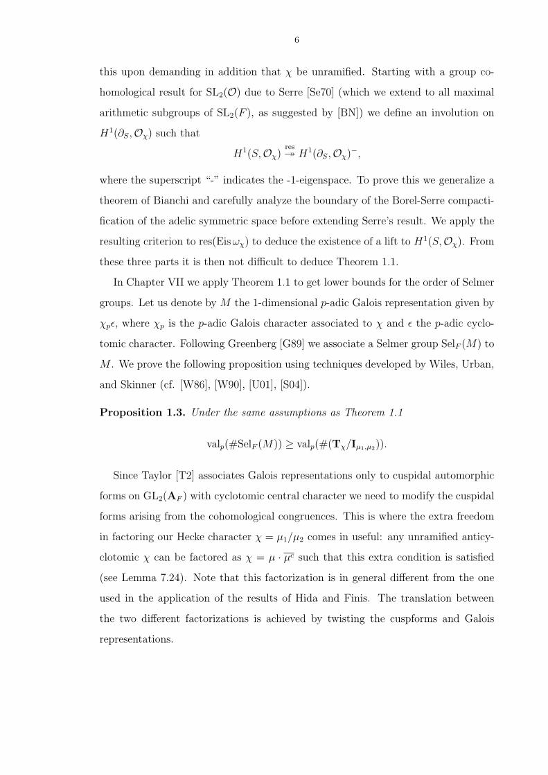
this upon demanding in addition that χ be unramified. Starting with a group co-

homological result for SL2(O) due to Serre [Se70] (which we extend to all maximal

arithmetic subgroups of SL2(F ), as suggested by [BN]) we define an involution on

H1(∂S,Oχ) such that

H1(S,Oχ)res³ H1(∂S,Oχ)−,

where the superscript “-” indicates the -1-eigenspace. To prove this we generalize a

theorem of Bianchi and carefully analyze the boundary of the Borel-Serre compacti-

fication of the adelic symmetric space before extending Serre’s result. We apply the

resulting criterion to res(Eis ωχ) to deduce the existence of a lift to H1(S,Oχ). From

these three parts it is then not difficult to deduce Theorem 1.1.

In Chapter VII we apply Theorem 1.1 to get lower bounds for the order of Selmer

groups. Let us denote by M the 1-dimensional p-adic Galois representation given by

χpε, where χp is the p-adic Galois character associated to χ and ε the p-adic cyclo-

tomic character. Following Greenberg [G89] we associate a Selmer group SelF (M) to

M . We prove the following proposition using techniques developed by Wiles, Urban,

and Skinner (cf. [W86], [W90], [U01], [S04]).

Proposition 1.3. Under the same assumptions as Theorem 1.1

valp(#SelF (M)) ≥ valp(#(Tχ/Iµ1,µ2)).

Since Taylor [T2] associates Galois representations only to cuspidal automorphic

forms on GL2(AF ) with cyclotomic central character we need to modify the cuspidal

forms arising from the cohomological congruences. This is where the extra freedom

in factoring our Hecke character χ = µ1/µ2 comes in useful: any unramified anticy-

clotomic χ can be factored as χ = µ · µc such that this extra condition is satisfied

(see Lemma 7.24). Note that this factorization is in general different from the one

used in the application of the results of Hida and Finis. The translation between

the two different factorizations is achieved by twisting the cuspforms and Galois

representations.

7

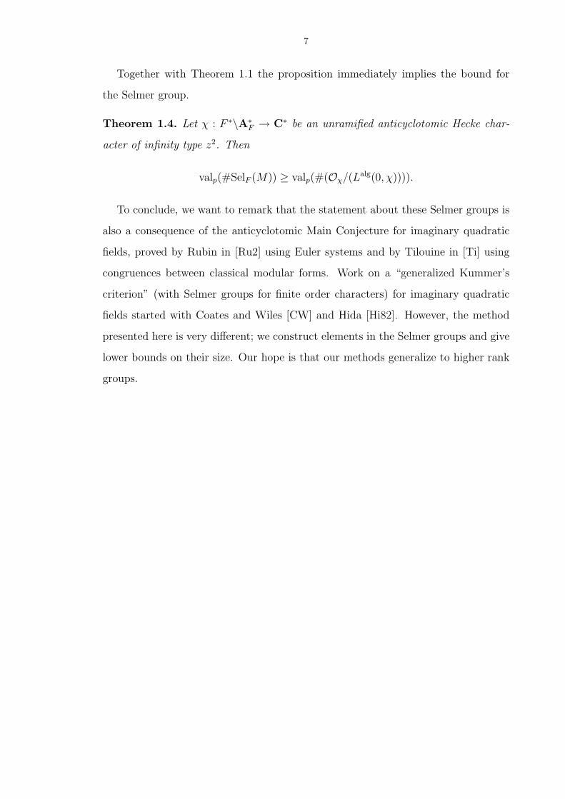
Together with Theorem 1.1 the proposition immediately implies the bound for

the Selmer group.

Theorem 1.4. Let χ : F ∗\A∗F → C∗ be an unramified anticyclotomic Hecke char-

acter of infinity type z2. Then

valp(#SelF (M)) ≥ valp(#(Oχ/(Lalg(0, χ)))).

To conclude, we want to remark that the statement about these Selmer groups is

also a consequence of the anticyclotomic Main Conjecture for imaginary quadratic

fields, proved by Rubin in [Ru2] using Euler systems and by Tilouine in [Ti] using

congruences between classical modular forms. Work on a “generalized Kummer’s

criterion” (with Selmer groups for finite order characters) for imaginary quadratic

fields started with Coates and Wiles [CW] and Hida [Hi82]. However, the method

presented here is very different; we construct elements in the Selmer groups and give

lower bounds on their size. Our hope is that our methods generalize to higher rank

groups.

CHAPTER II

Background

This chapter has two aims: to introduce notation and establish some conventions,

and to list facts (mostly without proof) that will be used in later chapters.

2.1 Basic notation

Let F be an imaginary quadratic field and σ its nontrivial automorphism. For

a place v of F let Fv be the completion of F at v. We write O for the ring of

integers of F , Ov for the closure of O in Fv, and O for∏

v finiteOv. We fix once

and for all an embedding F → F v for each place v of F . For each prime p we

also fix an embedding F p → C that is compatible with the fixed embeddings F →F p and F → C(= F∞). Complex conjugation is denoted by z 7→ z. We use

the notations A,Af and AF ,AF,f for the adeles and finite adeles of Q and F ,

respectively, and write A∗ and A∗F for the group of ideles. For an O-ideal m, define

U(m) =∏

v finite Uv(m) with Uv(m) = x ∈ Ov : x ≡ 1 mod mOv. Also let

FA(m) = x ∈ A∗F : xv = 1 if either v is infinite or mOv 6= Ov. Denote the class

group of F by Cl(F ) and the ray class group modulo m by Clm(F ). We write D for

the different of F and dF = Nm(D) for the (absolute) discriminant.

For any algebraic group H/Q and any ring A containing Q we write H(A) for the

group of A-valued points. We shall abbreviate H∞ = H(R).

8

9

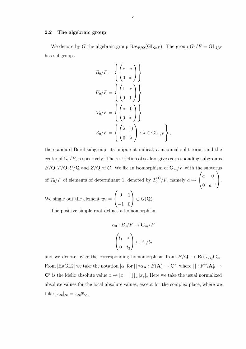
2.2 The algebraic group

We denote by G the algebraic group ResF/Q(GL2/F ). The group G0/F = GL2/F

has subgroups

B0/F =

∗ ∗

0 ∗

U0/F =

1 ∗

0 1

T0/F =

∗ 0

0 ∗

Z0/F =

λ 0

0 λ

: λ ∈ GL1/F

,

the standard Borel subgroup, its unipotent radical, a maximal split torus, and the

center of G0/F , respectively. The restriction of scalars gives corresponding subgroups

B/Q, T/Q, U/Q and Z/Q of G. We fix an isomorphism of Gm/F with the subtorus

of T0/F of elements of determinant 1, denoted by T(1)0 /F , namely a 7→

a 0

0 a−1

.

We single out the element w0 =

0 1

−1 0

∈ G(Q).

The positive simple root defines a homomorphism

α0 : B0/F → Gm/F

t1 ∗

0 t2

7→ t1/t2

and we denote by α the corresponding homomorphism from B/Q → ResF/QGm.

From [HaGL2] we take the notation |α| for | |αA : B(A) → C∗, where | | : F ∗\A∗F →

C∗ is the idelic absolute value x 7→ |x| = ∏v |xv|v Here we take the usual normalized

absolute values for the local absolute values, except for the complex place, where we

take |x∞|∞ = x∞x∞.

10

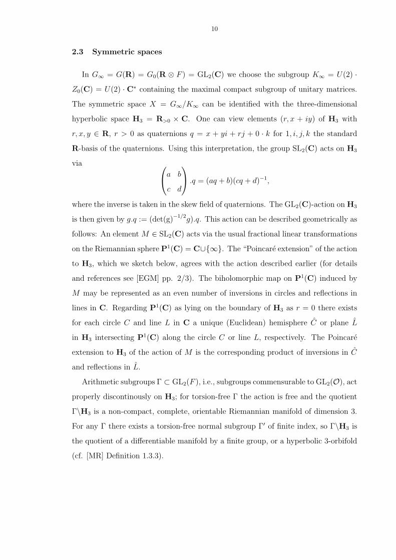
2.3 Symmetric spaces

In G∞ = G(R) = G0(R ⊗ F ) = GL2(C) we choose the subgroup K∞ = U(2) ·Z0(C) = U(2) · C∗ containing the maximal compact subgroup of unitary matrices.

The symmetric space X = G∞/K∞ can be identified with the three-dimensional

hyperbolic space H3 = R>0 × C. One can view elements (r, x + iy) of H3 with

r, x, y ∈ R, r > 0 as quaternions q = x + yi + rj + 0 · k for 1, i, j, k the standard

R-basis of the quaternions. Using this interpretation, the group SL2(C) acts on H3

via a b

c d

.q = (aq + b)(cq + d)−1,

where the inverse is taken in the skew field of quaternions. The GL2(C)-action on H3

is then given by g.q := (det(g)−1/2g).q. This action can be described geometrically as

follows: An element M ∈ SL2(C) acts via the usual fractional linear transformations

on the Riemannian sphere P1(C) = C∪∞. The “Poincare extension” of the action

to H3, which we sketch below, agrees with the action described earlier (for details

and references see [EGM] pp. 2/3). The biholomorphic map on P1(C) induced by

M may be represented as an even number of inversions in circles and reflections in

lines in C. Regarding P1(C) as lying on the boundary of H3 as r = 0 there exists

for each circle C and line L in C a unique (Euclidean) hemisphere C or plane L

in H3 intersecting P1(C) along the circle C or line L, respectively. The Poincare

extension to H3 of the action of M is the corresponding product of inversions in C

and reflections in L.

Arithmetic subgroups Γ ⊂ GL2(F ), i.e., subgroups commensurable to GL2(O), act

properly discontinously on H3; for torsion-free Γ the action is free and the quotient

Γ\H3 is a non-compact, complete, orientable Riemannian manifold of dimension 3.

For any Γ there exists a torsion-free normal subgroup Γ′ of finite index, so Γ\H3 is

the quotient of a differentiable manifold by a finite group, or a hyperbolic 3-orbifold

(cf. [MR] Definition 1.3.3).

11

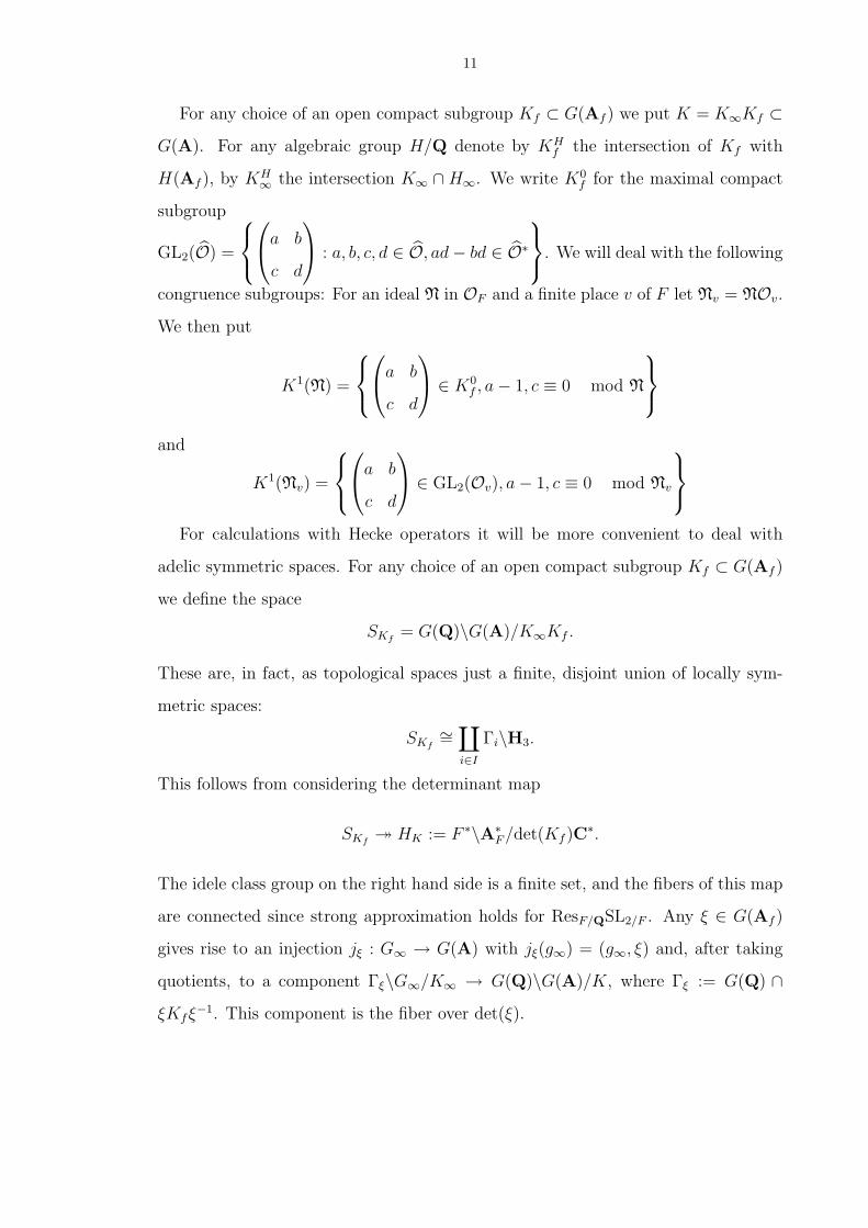
For any choice of an open compact subgroup Kf ⊂ G(Af ) we put K = K∞Kf ⊂G(A). For any algebraic group H/Q denote by KH

f the intersection of Kf with

H(Af ), by KH∞ the intersection K∞ ∩ H∞. We write K0

f for the maximal compact

subgroup

GL2(O) =

a b

c d

: a, b, c, d ∈ O, ad− bd ∈ O∗

. We will deal with the following

congruence subgroups: For an ideal N in OF and a finite place v of F let Nv = NOv.

We then put

K1(N) =

a b

c d

∈ K0

f , a− 1, c ≡ 0 mod N

and

K1(Nv) =

a b

c d

∈ GL2(Ov), a− 1, c ≡ 0 mod Nv

For calculations with Hecke operators it will be more convenient to deal with

adelic symmetric spaces. For any choice of an open compact subgroup Kf ⊂ G(Af )

we define the space

SKf= G(Q)\G(A)/K∞Kf .

These are, in fact, as topological spaces just a finite, disjoint union of locally sym-

metric spaces:

SKf∼=

∐i∈I

Γi\H3.

This follows from considering the determinant map

SKf³ HK := F ∗\A∗

F /det(Kf )C∗.

The idele class group on the right hand side is a finite set, and the fibers of this map

are connected since strong approximation holds for ResF/QSL2/F . Any ξ ∈ G(Af )

gives rise to an injection jξ : G∞ → G(A) with jξ(g∞) = (g∞, ξ) and, after taking

quotients, to a component Γξ\G∞/K∞ → G(Q)\G(A)/K, where Γξ := G(Q) ∩ξKfξ

−1. This component is the fiber over det(ξ).

12

2.4 Lie algebra

(References: [Ha79], [Ha82], [Ko]) The Lie algebra g = Lie(G/Q) is a Q-vector

space and we define g∞ = g ⊗Q R. Then g∞ is the Lie algebra of the real group

G∞ = G(R) = GL2(C) and so equals the two-by-two complex matrices M2(C)

thought of as an R-vector space. It carries a positive semidefinite K∞-invariant

form, the Killing form

〈X,Y 〉 =1

16trace(adX · adY ),

and with respect to this form we have an orthogonal decomposition g∞ = k∞ ⊕ p,

where k∞ = Lie(K∞) and

p = RH ⊕RE1 ⊕RE2 := R

1 0

0 −1

⊕R

0 1

1 0

⊕R

0 i

−i 0

.

The group K∞ acts on p by the adjoint action. Let P/Q be any Borel subgroup of

G. Under the action of KP∞ we have a canonical decomposition of p = p0,P ⊕ p1,P ,

where p0,P is the 1-dimensional subspace on which KP∞ acts trivially and p1,P is 2-

dimensional and an irreducible KP∞-module. In the case P = B this decomposition

becomes p = RH ⊕ (RE1 ⊕RE2).

Let S± := 12(±E1 ⊗R 1− E2 ⊗R i) ∈ pC and denote by S± the dual vectors with

respect to the Killing form.

The adjoint action of k∞ =

α β

−β α

∈ SU2(C) ⊂ K∞ on pC is given by

(2.1) k∞.

S+

H

S−

=

α2 αβ β2

−2αβ αα− ββ 2αβ

β2 −αβ α2

S+

H

S−

.

In the center of the enveloping algebra of g∞ ⊗R C we have the two Casimir

operators D′ = X ′Y ′ + Y ′X ′ + H ′2/2 and D′′ = X ′′Y ′′ + Y ′′X ′′ + H ′′2/2, where

X =

0 1

0 0

, Y =

0 0

1 0

, where A′.f = (∂/∂z)z=0((1 + zA).f) and A′′.f =

(∂/∂z)z=0((1 + zA).f) for each matrix A of g∞.

13

Denote the Lie algebra over Q corresponding to T by t, the Lie algebra over F

corresponding to T0 by t0, and the Lie algebra of T (R) by t∞. Similarly use u and b

for the Lie algebras of U and B with the same convention on subscripts.

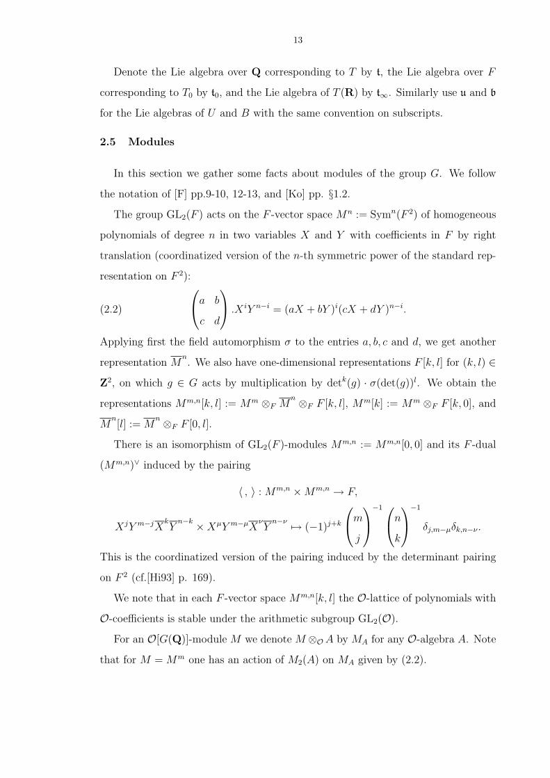
2.5 Modules

In this section we gather some facts about modules of the group G. We follow

the notation of [F] pp.9-10, 12-13, and [Ko] pp. §1.2.

The group GL2(F ) acts on the F -vector space Mn := Symn(F 2) of homogeneous

polynomials of degree n in two variables X and Y with coefficients in F by right

translation (coordinatized version of the n-th symmetric power of the standard rep-

resentation on F 2):

(2.2)

a b

c d

.X iY n−i = (aX + bY )i(cX + dY )n−i.

Applying first the field automorphism σ to the entries a, b, c and d, we get another

representation Mn. We also have one-dimensional representations F [k, l] for (k, l) ∈

Z2, on which g ∈ G acts by multiplication by detk(g) · σ(det(g))l. We obtain the

representations Mm,n[k, l] := Mm ⊗F Mn ⊗F F [k, l], Mm[k] := Mm ⊗F F [k, 0], and

Mn[l] := M

n ⊗F F [0, l].

There is an isomorphism of GL2(F )-modules Mm,n := Mm,n[0, 0] and its F -dual

(Mm,n)∨ induced by the pairing

〈 , 〉 : Mm,n ×Mm,n → F,

XjY m−jXkY

n−k ×XµY m−µXνY

n−ν 7→ (−1)j+k

m

j

−1

n

k

−1

δj,m−µδk,n−ν .

This is the coordinatized version of the pairing induced by the determinant pairing

on F 2 (cf.[Hi93] p. 169).

We note that in each F -vector space Mm,n[k, l] the O-lattice of polynomials with

O-coefficients is stable under the arithmetic subgroup GL2(O).

For an O[G(Q)]-module M we denote M ⊗O A by MA for any O-algebra A. Note

that for M = Mm one has an action of M2(A) on MA given by (2.2).

14

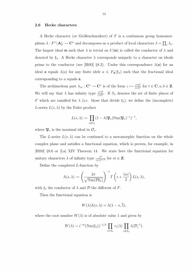
2.6 Hecke characters

A Hecke character (or Großencharakter) of F is a continuous group homomor-

phism λ : F ∗\A∗F → C∗ and decomposes as a product of local characters λ =

∏v λv.

The largest ideal m such that λ is trivial on U(m) is called the conductor of λ and

denoted by fλ. A Hecke character λ corresponds uniquely to a character on ideals

prime to the conductor (see [Hi93] §8.2). Under this correspondence λ(a) for an

ideal a equals λ(a) for any finite idele a ∈ FA(fλ) such that the fractional ideal

corresponding to a equals a.

The archimedean part λ∞ : C∗ → C∗ is of the form z 7→ zazb

(zz)t for t ∈ C, a, b ∈ Z.

We will say that λ has infinity type zazb

(zz)t . If Sλ denotes the set of finite places of

F which are ramified for λ (i.e. those that divide fλ), we define the (incomplete)

L-series L(s, λ) by the Euler product

L(s, λ) :=∏

v/∈Sλ

(1− λ(Pv)Nm(Pv)−s)−1,

where Pv is the maximal ideal in Ov.

The L-series L(s, λ) can be continued to a meromorphic function on the whole

complex plane and satisfies a functional equation, which is proven, for example, in

[Hi93] §8.6 or [La] XIV Theorem 14. We state here the functional equation for

unitary characters λ of infinity type zm

(zz)m/2 for m ∈ Z:

Define the completed L-function by

Λ(s, λ) :=

(2π√

Nm(Dfλ)

)−s

Γ

(s +

|m|2

)L(s, λ),

with fλ the conductor of λ and D the different of F .

Then the functional equation is

W (λ)Λ(s, λ) = Λ(1− s, λ),

where the root number W (λ) is of absolute value 1 and given by

W (λ) = i−m(Nm(fλ))−1/2

∏v∈Sλ

τv(λ)∏

v/∈Sλ

λ(D−1v ).

15

Here the Gauss sum τv is given by

τv(λv) =∑

ε∈O∗v/(1+fλ,v)

(λe)(επ−ordv(fλD))

for e the standard additive character e(x) = exp(−2πi[trFv/Ql]`), where ` is the

residual characteristic of v and [x]` denotes the `-fraction part for x ∈ Q`.

If the infinity type of λ is zn, the functional equation takes the following form:

The completed L-series is now

Λ(s, λ) :=

(2π√

Nm(Dfλ)

)−s

Γ(s)L(s, λ).

Denoting by λ the unitary character λ| · |−n/2 we get

(2.3) W (λ)Λ(1− n− s, λ) = Λ(s, λ).

Define the character λc by λc(x) = λ(σ(x)). Since σ just permutes the Euler

factors we have L(s, λ) = L(s, λc).

We will use the following result of Shimura, Katz, Hida and Tilouine about the

special L-value for s = 0:

Theorem 2.1. Let p be a rational prime that splits in F , p one of the prime ideals

in F lying above it, and λ an algebraic Hecke character with conductor prime to p

and of infinity type zk(

zz

)`, where k and ` are integers satisfying either k > 0 and

` ≥ 0 or k ≤ 1 and ` ≥ 1− k. Then there exists a complex period Ω, independent of

λ, such that

Lalg(0, λ) := Ω−k−2`

(2π√dF

)`

Γ(k + `)(1− λ(p))(1− λ∗(p))L(0, λ) ∈ O,

where O is the integer ring of an unramified finite extension of Fp, dF = Nm(D) is

the absolute discriminant of F and λ∗(p) = λ(p)−1Nm(p).

References. Shimura showed that this normalization is algebraic. Together, [K76]

Chapters 4 and 8, [K78] Theorem 5.3.0, and [HT] Theorem II show that it is a p-adic

integer in F p. With our fixed embedding F → F p this shows that the value lies in

a finite extension of Fp and is p-integral. See also [Hi04a] Theorem 1.1 and [dS] II

Theorem 4.12 and 4.14.

16

We will be working with Hecke characters λ of type (A0), i.e., characters with

infinity type zazb with a, b ∈ Z (cf. [We55]). For such characters Q(Im(λf )) is a

number field and one can attach to λ a p-adic Galois character of Gal(F/F ), its

p-adic avatar (cf. [Hi82] p. 248):

Let m be the conductor of λ and let K be the finite extension of F containing

λ(x) for all x ∈ FA(m) and all conjugates of F over Q. Fix a finite place v of K

and write p for its residual characteristic. For x ∈ F ∗p = (F ⊗Q Qp)

∗ =∏

w|p F ∗w

define λ∞(x) using the extensions of the embeddings F → K to Fw → Kv and λ∞.

Now let λv : F ∗\A∗F /U(m)(p)F ∗

∞ → K∗v be the unique continuous character such

that λv(x) = λ(x) if x ∈ FA(mp) and λv(xp) = λ(xp)λ∞(xp) for all xp ∈ F ∗p . Using

the Artin reciprocity map of class field theory, this gives rise to a Galois character

λp : Gal(F (mp∞)/F ) → K∗v , where F (mp∞) denotes the ray class field of conductor

mp∞ and p is the prime of F lying below v.

2.7 Automorphic forms

We want to use congruences between modular forms over imaginary quadratic

fields. There are various ways of thinking of these:

• real analytic functions on hyperbolic three-space H3 (Maass forms)

• automorphic representations of GL2(AF )

• certain cohomology classes in the cohomology of quotients of H3 by congruence

subgroups Γ ⊂ GL2(O).

They are best susceptible to computation in the latter incarnation, and we will

mainly be handling them in this form, but since we later want to work with auto-

morphic forms and representations, we will recall their definition here (following the

description in [U95], [U98]):

For a compact open subgroup Kf ⊂ G(Af ), we call a function f : G(A) → M2n+2C

an automorphic form for Kf of weight n ≥ 0, if it satisfies conditions (1)-(7) in the

following list. If it also satisfies (8), we call it a cuspidal automorphic form.

17

(1) f(γg) = f(g) for all γ ∈ G(Q)

(2) f(gz∞) = f(g) · |z∞|−n∞ for all z∞ ∈ Z0(C)

(3) f(gk∞) = k∞.f(g) for all k∞ ∈ U(2)

(4) f(gk) = f(g) for all k ∈ Kf

(5) With respect to any U2(C)-invariant norm on M2n+2C , f × |det|nAF

is square inte-

grable on SGKf

.

(6) f is C∞ and of moderate growth in its archimedean component

(7) f is an eigenvector of the Casimir operators D′ and D′ with eigenvalue n + n2/2

(see [We71], pp. 67-68).

(8) For each g ∈ G(A), one has

∫

U(Q)\U(A)

f(ug)du = 0.

We will denote the space of automorphic forms for Kf of weight n by Mn(Kf ,C) and

the subspace of cuspidal forms by Sn(Kf ,C). For each continuous ω : F ∗\A∗F → C∗,

we further denote by Sn(Kf , ω,C) the space of forms satisfying in addition f(gz) =

f(g)ω(z) for each z ∈ Z(A).

G(A) acts on these spaces by right translation. As explained in [U95] §3.1,

(2.4) Sn(Kf ,C) ∼=⊕

Π

VKf

Πf,

where the sum is over cuspidal automorphic representations Π with Π∞ isomorphic

to the principal series representation of GL2(C) corresponding to the character

t1 ∗

0 t2

7→

(t1

|t1|1/2∞

)n+1 (|t2|1/2

∞t2

)n+1

· |t1t2|−n/2∞ .

For Sn(Kf , ω,C) one has a similar decomposition restricting above sum to the cusp-

idal automorphic representations with central character ω (to be defined later). For

the exact definition of cuspidal automorphic representations we refer to [Gel]. We re-

call here only that a cuspidal automorphic representation Π factors as Π = Π∞⊗Πf

18

for Π∞ a representation of GL2(C) and Πf an irreducible representation of GL2(Af )

whose space we denote by VΠf. The multiplicity one theorem of Jacquet and Lang-

lands says that each isomorphism class of automorphic representations occurs only

once in this decomposition. The GL2(Af )-representation Πf further factors as Πf =⊗

v Πv with each Πv an irreducible admissible representation of GL2(Fv). All but

finitely many Πv (v /∈ S for some finite set of places S) are unramified, i.e. VΠv has

a nonzero vector fixed by GL2(Ov). A representation Πv : GL2(Fv) → GL(V ) for a

complex vector space V is called admissible if (i) every vector v ∈ V is fixed by some

open subgroup of GL2(Fv), and (ii) for every open compact subgroup Kv of GL2(Fv)

the subspace of vectors in V fixed by Kv is finite dimensional.

If Kv is an open compact subgroup of GL2(Fv) we write V Kv for the subspace of

vectors fixed by Kv. For open compact subgroups Kv and K ′v and an element g of

GL2(Fv) we define the Hecke operator [KvgK ′v] : V K′

v → V Kv by

[KvgKv′]φ =

∑i

h−1i .φ

where KvgKv′ =

∐i Kv

′hi. Similarly, for open compact subgroups Kf , Kf′ of GL2(Af )

and g ∈ GL2(Af ), one has a Hecke action of [KfgKf′] on V

Kf

Πfand so, by (2.4),

on Sn(Kf ,C). For Kf = Kf′ = K1(N) define Tv = [K1(N)

1 0

0 πv

K1(N)]

for all finite places v and Sv = [K1(N)

πv 0

0 πv

K1(N)] for places v not divid-

ing N, where πv is a uniformizer of Fv. If φ = ⊗wφw ∈ VK1(N)Πf

then Tv and Sv

only act on φv. The operator Tv, for example, therefore has the same action as

[K1(Nv)

1 0

0 πv

K1(Nv)]. One can show that if Πv is unramified (i.e., v /∈ S)

then VGL2(Ov)Πv

is 1-dimensional (see [Cas] and Section 3.2). This implies that any

φ = ⊗wφw ∈ VKf

Πfwith Kf,v = GL2(Ov) has the same eigenvalue for Tv since φv is

unique up to scalar. We will denote it by av(Π).

Note also that by Schur’s Lemma each Π has a central character ω = ⊗ωv with

ωv giving the action of the center of each GL2(Fv). Note that if Πv is unramified

19

then ωv(πv) gives the inverse of the eigenvalue of Πv for Sv.

2.8 Borel-Serre compactification

In general, the manifolds Γ\H3 and SKffrom Section 2.3 are not compact. There

are several ways to compactify them, but the one most convenient for cohomological

considerations is the Borel-Serre compactification (cf. [BS]). This compactification

gives manifolds with corners and we will denote them by Γ\H3 and SKf, respectively.

In fact, one first considers the Borel-Serre compactification H3 of H3, a manifold

with (countably many) corners. As a set, H3 is given as union of H3 with boundary

faces e(P ) = H3/AP∼= UP (R), one for each rational Borel subgroup P of G, where

UP denotes its unipotent radical and AP the identity component of P (R)/UP (R),

and the action of AP on H3 is the geodesic action (cf. [BS]). The set is given a

G(Q)-invariant topology.

In our situation this can be described very explicitely by viewing the boundary

faces e(P ) as “horospheres minus a point” (see [BJ] III.5.15, [Ko] §1.4.4). This means

that we view H3 as

H3 = H3 ∪⋃

x∈P1(F )

(P1(C)− x).

The group G(Q) acts on⋃

x∈P1(F )(P1(C) − x) by mapping w ∈ P1(C) − x

to γw ∈ P1(C) − γx for γ ∈ G(Q). Together with the usual action on H3 we

therefore have defined an action of G(Q) on H3. We equip H3 now with a G(Q)-

invariant topology. On H3 we take the product topology of (0,∞) × C, which

agrees with the natural topology coming from G∞/K∞ ∼= H3 = R>0 × C. For

x = [0 : 1](= ∞) we identify P1(C) − x with ∞ ×C via [1 : z] 7→ ∞ × z.We then give H3 ∪ (P1(C) − x) the product topology of (0,∞] ×C. One checks

that the group B(Q) operates topologically on H3 ∪ (P1(C) − x). The topology

on H3 is then defined so that each γ ∈ G(Q) acts as a topological automorphism.

If we view the other cusps [1 : z] ∈ P1(F ) as points (0, z) in the complex plane

(0, c)|c ∈ C ⊂ R≥0 × C attached to H3 then neighborhoods of ∞ of the form

(r, z) : r ≥ r0 correspond to Euclidean balls in H3 tangent to 0 × C at (0, z).

20

Such a ball of radius R can be identified with (P1(C) − [1 : z]) × (0, R] and the

boundary face P1(C)−[1 : z] is added as (P1(C)−[1 : z])×0. (This is where

the terminology “horosphere” comes from, see also [MR] p. 54.)

Using reduction theory one shows that H3 is Hausdorff. The natural inclusions

of H3 and e(P ) into H3 are embeddings of real manifolds. Moreover, H3 is open

and each e(P ) is closed and the arithmetic subgroup Γ ⊂ G(Q) acts properly discon-

tinuously on H3 and H3 \H3. The quotient Γ\H3 is a Hausdorff compactification

of Γ\H3, also denoted by Γ\H3. Its boundary ∂(Γ\H3) is a finite union of tori

ΓP\e(P ), with ΓP = Γ ∩ P (Q), for a set of representatives of Γ-conjugacy classes

of Borel subgroups (equivalently of P1(F )/Γ). Furthermore, e′(P ) := ΓP\e(P ) is

homotopy equivalent to ΓP\H3.

The Borel-Serre compactification of the adelic symmetric space is given by

(2.5) SKf=

∐

[det(ξ)]∈HK

Γξ\H3 =∐

[det(ξ)]∈HK

Γξ\H3 t[η]∈P1(F )/ΓξΓξ,Bη\e(Bη),

with HK = A∗F /det(K)F ∗, Γξ = G(Q) ∩ ξKfξ

−1 for ξ ∈ G(Af ), and Bη(Q) =

η−1B(Q)η for η ∈ G(Q). The topology is such that SKf

i→ SKf

is a homotopy

equivalence.

For a very concise description for the Borel-Serre compactification of the adelic

symmetric space agreeing with the compactification of its connected components

Γξ\H3 sketched above, we refer to [HaGL2] §2.1. He shows that ∂SKfis homotopy

equivalent to

∂SKf:= B(Q)\G(Q)/KfK∞ ∼=

∐

[det(ξ)]∈HK

∐

[η]∈P1(F )/Γξ

Γξ,Bη\H3,

where the boundary component Γξ,Bη\H3 gets embedded in ∂SKfvia g∞ 7→ jη,ξ(g∞) :=

η(g∞, ξ) (see [Ha82] p. 110). We note that together with the embeddings jξ defined

in Section 2.3 we have the following commutative diagram:

g∞∈Γξ,Bη\H3

jη,ξ−−−→ B(Q)\G(A)/KfK∞ = ∂SKfyy

yprojection

g∞∈ Γξ\H3

jξ−−−→ G(Q)\G(A)/KfK∞ = SKf

21

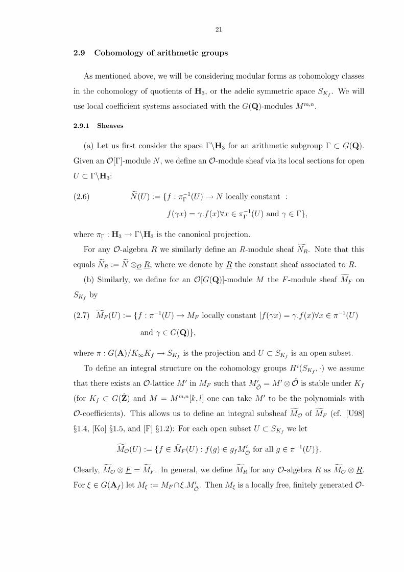
2.9 Cohomology of arithmetic groups

As mentioned above, we will be considering modular forms as cohomology classes

in the cohomology of quotients of H3, or the adelic symmetric space SKf. We will

use local coefficient systems associated with the G(Q)-modules Mm,n.

2.9.1 Sheaves

(a) Let us first consider the space Γ\H3 for an arithmetic subgroup Γ ⊂ G(Q).

Given an O[Γ]-module N , we define an O-module sheaf via its local sections for open

U ⊂ Γ\H3:

N(U) := f : π−1Γ (U) → N locally constant :(2.6)

f(γx) = γ.f(x)∀x ∈ π−1Γ (U) and γ ∈ Γ,

where πΓ : H3 → Γ\H3 is the canonical projection.

For any O-algebra R we similarly define an R-module sheaf NR. Note that this

equals NR := N ⊗O R, where we denote by R the constant sheaf associated to R.

(b) Similarly, we define for an O[G(Q)]-module M the F -module sheaf MF on

SKfby

MF (U) := f : π−1(U) → MF locally constant |f(γx) = γ.f(x)∀x ∈ π−1(U)(2.7)

and γ ∈ G(Q),

where π : G(A)/K∞Kf → SKfis the projection and U ⊂ SKf

is an open subset.

To define an integral structure on the cohomology groups H i(SKf, ·) we assume

that there exists an O-lattice M ′ in MF such that M ′O = M ′⊗ O is stable under Kf

(for Kf ⊂ G(Z) and M = Mm,n[k, l] one can take M ′ to be the polynomials with

O-coefficients). This allows us to define an integral subsheaf MO of MF (cf. [U98]

§1.4, [Ko] §1.5, and [F] §1.2): For each open subset U ⊂ SKfwe let

MO(U) := f ∈ MF (U) : f(g) ∈ gfM′O for all g ∈ π−1(U).

Clearly, MO ⊗ F = MF . In general, we define MR for any O-algebra R as MO ⊗ R.

For ξ ∈ G(Af ) let Mξ := MF ∩ξ.M ′O. Then Mξ is a locally free, finitely generated O-

22

module with an action by Γξ = G(Q)∩ ξKfξ−1 and j∗ξ (MO) ∼= Mξ for jξ : Γξ\H3 →

SKffrom Section 2.3.

(c) Lastly, we define R-module sheaves MR on ∂SKf= B(Q)\G(A)/KfK∞ as

pullbacks of the corresponding sheaves on SKfvia the canonical projection. In this

case one has the relation j∗η,ξ(MO) ∼= Mξ for jη,ξ : Γξ,Bη\H3 → ∂SKffrom Section

2.8.

2.9.2 Sheaf cohomology and group cohomology

(a) For the definitions of sheaf cohomology we refer to Chapter 3 of [Hart], Chapter

II of [B67], and [Go]. For a sheaf F on a topological space X, we denote by H i(X,F)

(resp. H ic(X,F)) the i-th cohomology group of F (resp. with compact support), and

the interior cohomology, i.e., the image of H ic(X,F) in H i(X,F), by H i

! (X,F).

For the rest of this subsection let M be an O[G(Q)]-module and R an O-algebra.

The R-modules H i(SKf, MR) are finitely generated. Since SKf

i→ SKf

is a homotopy

equivalence, we have a canonical isomorphism

H i(SKf, MR) ∼= H i(SKf

, i∗MR)

and in what follows we will replace i∗MR by MR and also write MR for the sheaf

j∗i∗MR on ∂SKf, for j : ∂SKf

→ SKf. By [HaGL2] §2.1 we have

H i(∂SKf, M) ∼= H i(∂SKf

, M).

The decomposition of the adelic symmetric space into connected components gives

rise to canonical isomorphisms (see [Ko] §1.6 and [F] §1.2)

H i(SKf, MR) ∼=

⊕

[det(ξ)]∈HK

H i(Γξ\H3, Mξ ⊗R)

and

H i(∂SKf, MR) ∼=

⊕

[det(ξ)]∈HK

⊕

[η]∈P1(F )/Γξ

H i(Γξ,Bη\H3, Mξ ⊗R).

The above cohomology groups and isomorphisms are all functorial in R.

23

From the short exact sequence

0 → i!MR → i∗MR → i∗MR/i!MR → 0

and i∗MR/i!MR∼= j∗(j∗i∗MR) we get a long exact sequence (functorial in R)

(2.8)

. . . → H1c (SKf

, MR) → H1(SKf, MR)

res→ H1(∂SKf, MR)

∂→ H2c (SKf

, MR) → . . .

We have an operation of a Hecke algebra on the cohomology groups H i(SKf, MR)

and H i(∂SKf, MR): For x ∈ G(Af ) such that x ·M ′ ⊂ M ′ (where M ′ is an O-lattice

such that M ′O is stable under Kf ) one defines

[KfxKf ] : H i?(SKf

, MR) → H i?(SKf

, MR)

by

[KfxKf ] = trKf ,Kf∩xKf x−1 rx resKf ,Kf∩x−1Kf x,

where ? can be ∅ or c, rx is the map from H i?(SKf∩x−1Kf x, MR) to H i

?(SKf∩xKf x−1 , MR)

induced by right multiplication by x−1, tr denotes a transfer morphism and res a

restriction map (the definition for ∂SKfis similar). We refer to [U98] §1.4.4 for the

details. These actions are compatible with the restriction map res in the long exact

sequence (2.8), and so we also get an action on H i! (SKf

, MR).

For Kf = K1(N) we again single out the operators Tv = [K1(N)

1 0

0 πv

K1(N)]

and Sv = [K1(N)

πv 0

0 πv

K1(N)] (diamond operator, [U98] §1.4.5).

(b) If G is a group and A an abelian group with an action by G we denote by

H i(G,A) the i-th cohomology group of G with coefficients in A. This is defined as

the i-th right derived functor of the functor A 7→ AG. We consider the resolution of

A given by the complex

0 → Aε→ A0(G,A)

d0→ A1(G,A)d1→ . . .

di−1→ Ai(G,A)di→ . . . ,

where Ai(G,A) = Maps(Gi+1, A), ε(a) is the constant function equal to a on G and

di(f)(x0, . . . , xi+1) =i+1∑j=0

(−1)jf(x0, . . . , xj, . . . , xi+1),

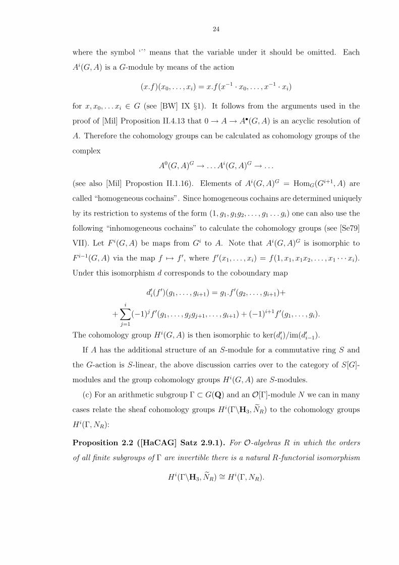
24

where the symbol ‘ ’ means that the variable under it should be omitted. Each

Ai(G, A) is a G-module by means of the action

(x.f)(x0, . . . , xi) = x.f(x−1 · x0, . . . , x−1 · xi)

for x, x0, . . . xi ∈ G (see [BW] IX §1). It follows from the arguments used in the

proof of [Mil] Proposition II.4.13 that 0 → A → A•(G,A) is an acyclic resolution of

A. Therefore the cohomology groups can be calculated as cohomology groups of the

complex

A0(G,A)G → . . . Ai(G,A)G → . . .

(see also [Mil] Propostion II.1.16). Elements of Ai(G,A)G = HomG(Gi+1, A) are

called “homogeneous cochains”. Since homogeneous cochains are determined uniquely

by its restriction to systems of the form (1, g1, g1g2, . . . , g1 . . . gi) one can also use the

following “inhomogeneous cochains” to calculate the cohomology groups (see [Se79]

VII). Let F i(G,A) be maps from Gi to A. Note that Ai(G,A)G is isomorphic to

F i−1(G,A) via the map f 7→ f ′, where f ′(x1, . . . , xi) = f(1, x1, x1x2, . . . , x1 · · ·xi).

Under this isomorphism d corresponds to the coboundary map

d′i(f′)(g1, . . . , gi+1) = g1.f

′(g2, . . . , gi+1)+

+i∑

j=1

(−1)jf ′(g1, . . . , gjgj+1, . . . , gi+1) + (−1)i+1f ′(g1, . . . , gi).

The cohomology group H i(G, A) is then isomorphic to ker(d′i)/im(d′i−1).

If A has the additional structure of an S-module for a commutative ring S and

the G-action is S-linear, the above discussion carries over to the category of S[G]-

modules and the group cohomology groups H i(G,A) are S-modules.

(c) For an arithmetic subgroup Γ ⊂ G(Q) and an O[Γ]-module N we can in many

cases relate the sheaf cohomology groups H i(Γ\H3, NR) to the cohomology groups

H i(Γ, NR):

Proposition 2.2 ([HaCAG] Satz 2.9.1). For O-algebras R in which the orders

of all finite subgroups of Γ are invertible there is a natural R-functorial isomorphism

H i(Γ\H3, NR) ∼= H i(Γ, NR).

25

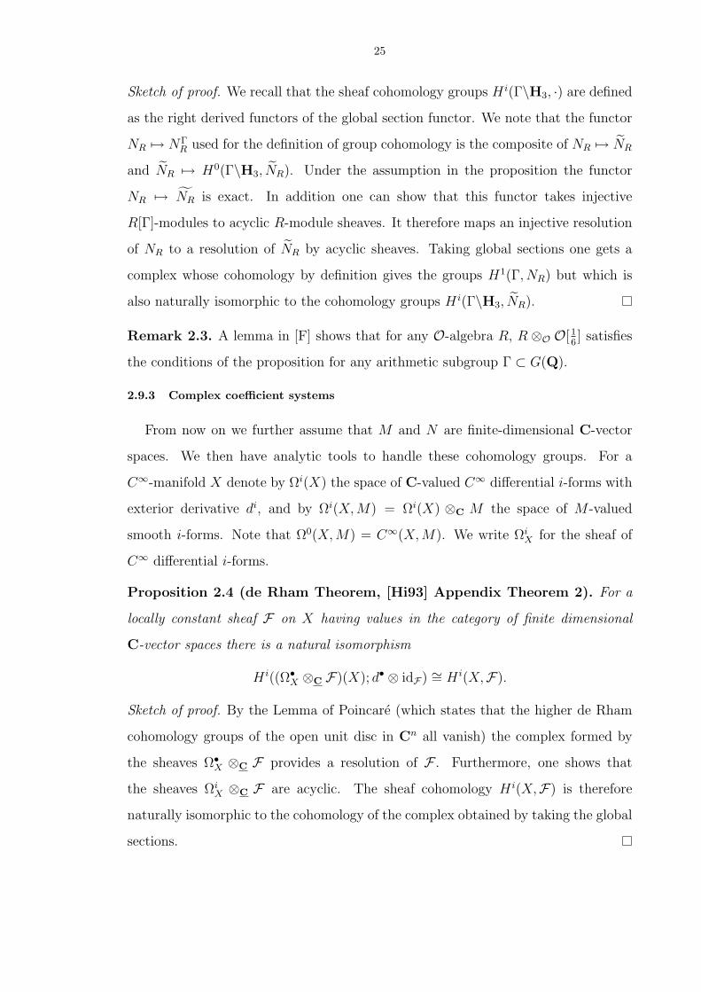
Sketch of proof. We recall that the sheaf cohomology groups H i(Γ\H3, ·) are defined

as the right derived functors of the global section functor. We note that the functor

NR 7→ NΓR used for the definition of group cohomology is the composite of NR 7→ NR

and NR 7→ H0(Γ\H3, NR). Under the assumption in the proposition the functor

NR 7→ NR is exact. In addition one can show that this functor takes injective

R[Γ]-modules to acyclic R-module sheaves. It therefore maps an injective resolution

of NR to a resolution of NR by acyclic sheaves. Taking global sections one gets a

complex whose cohomology by definition gives the groups H1(Γ, NR) but which is

also naturally isomorphic to the cohomology groups H i(Γ\H3, NR).

Remark 2.3. A lemma in [F] shows that for any O-algebra R, R ⊗O O[16] satisfies

the conditions of the proposition for any arithmetic subgroup Γ ⊂ G(Q).

2.9.3 Complex coefficient systems

From now on we further assume that M and N are finite-dimensional C-vector

spaces. We then have analytic tools to handle these cohomology groups. For a

C∞-manifold X denote by Ωi(X) the space of C-valued C∞ differential i-forms with

exterior derivative di, and by Ωi(X,M) = Ωi(X) ⊗C M the space of M -valued

smooth i-forms. Note that Ω0(X,M) = C∞(X, M). We write ΩiX for the sheaf of

C∞ differential i-forms.

Proposition 2.4 (de Rham Theorem, [Hi93] Appendix Theorem 2). For a

locally constant sheaf F on X having values in the category of finite dimensional

C-vector spaces there is a natural isomorphism

H i((Ω•X ⊗C F)(X); d• ⊗ idF) ∼= H i(X,F).

Sketch of proof. By the Lemma of Poincare (which states that the higher de Rham

cohomology groups of the open unit disc in Cn all vanish) the complex formed by

the sheaves Ω•X ⊗C F provides a resolution of F . Furthermore, one shows that

the sheaves ΩiX ⊗C F are acyclic. The sheaf cohomology H i(X,F) is therefore

naturally isomorphic to the cohomology of the complex obtained by taking the global

sections.

26

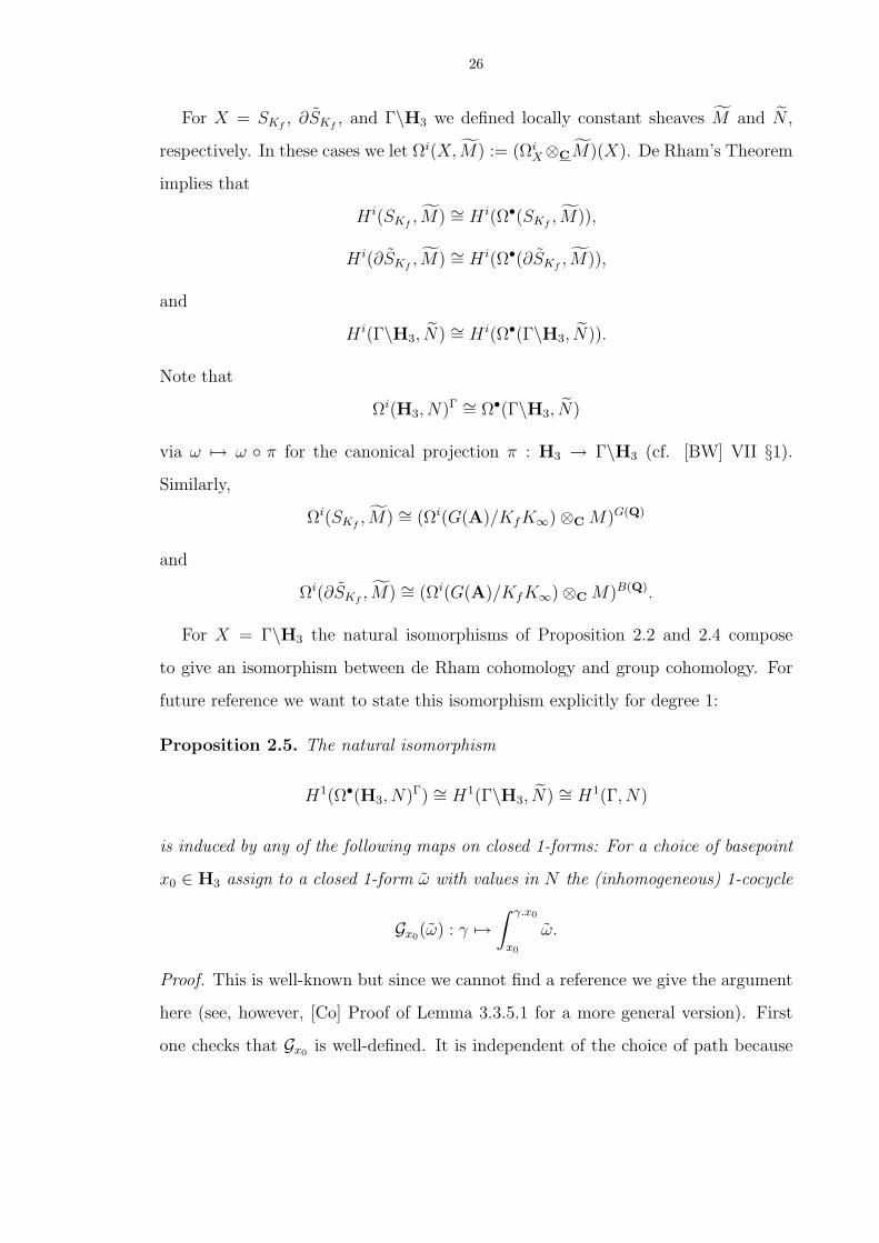
For X = SKf, ∂SKf

, and Γ\H3 we defined locally constant sheaves M and N ,

respectively. In these cases we let Ωi(X, M) := (ΩiX⊗CM)(X). De Rham’s Theorem

implies that

H i(SKf, M) ∼= H i(Ω•(SKf

, M)),

H i(∂SKf, M) ∼= H i(Ω•(∂SKf

, M)),

and

H i(Γ\H3, N) ∼= H i(Ω•(Γ\H3, N)).

Note that

Ωi(H3, N)Γ ∼= Ω•(Γ\H3, N)

via ω 7→ ω π for the canonical projection π : H3 → Γ\H3 (cf. [BW] VII §1).

Similarly,

Ωi(SKf, M) ∼= (Ωi(G(A)/KfK∞)⊗C M)G(Q)

and

Ωi(∂SKf, M) ∼= (Ωi(G(A)/KfK∞)⊗C M)B(Q).

For X = Γ\H3 the natural isomorphisms of Proposition 2.2 and 2.4 compose

to give an isomorphism between de Rham cohomology and group cohomology. For

future reference we want to state this isomorphism explicitly for degree 1:

Proposition 2.5. The natural isomorphism

H1(Ω•(H3, N)Γ) ∼= H1(Γ\H3, N) ∼= H1(Γ, N)

is induced by any of the following maps on closed 1-forms: For a choice of basepoint

x0 ∈ H3 assign to a closed 1-form ω with values in N the (inhomogeneous) 1-cocycle

Gx0(ω) : γ 7→∫ γ.x0

x0

ω.

Proof. This is well-known but since we cannot find a reference we give the argument

here (see, however, [Co] Proof of Lemma 3.3.5.1 for a more general version). First

one checks that Gx0 is well-defined. It is independent of the choice of path because

27

dω = 0. Also it is easy to check that the class of the cocycle is independent of the

choice of x0.

Since the functor N → NΓ is left-exact and by Propositions 2.2 and 2.4 the

functors N 7→ H i(Ω•(H3, N)Γ) and N 7→ H i(Γ, N) are erasable functors on C[Γ]-

modules (see [Hart] III.1 for the definition of erasable additive functors). This implies

that both

(H i(Ω•(H3, ·)Γ))i≥0 and (H i(Γ, ·))i≥0

are universal δ-functors. (We again refer to [Hart] III.1 for the definition and proper-

ties of δ-functors.) By the universality of both δ-functors there is a unique sequence

of isomorphisms H i(Ω•(H3, ·)Γ) → H i(Γ, ·) for each i ≥ 0, starting with the canoni-

cal isomorphism in degree 0, which commute with the connecting homomorphism δi

for each short exact sequence of C[Γ]-modules. It suffices therefore to show that the

map on closed 1-forms given above defines a morphism H1(Ω•(H3, ·)Γ) → H1(Γ, ·)extending the one in degree 0.

As we recalled above, H1(Γ, N) is calculated by taking Γ-invariants of the acyclic

resolution N → A•(Γ, N) and computing the cohomology of the resulting complex.

The de Rham cohomology group is calculated as the cohomology of the complex

NΓ → Ω•(Γ\H3, N) = Ω•(H3, N)Γ. This is the complex of Γ-invariants of the

complex N → Ω•(H3, N). Since H3 is contractible the Poincare Lemma mentioned

above in Proposition 2.4 implies that this latter complex is exact and therefore a

resolution of N . Note also that both resolutions are functorial in N .

For any x0 ∈ H3 the morphism f 0 : C∞(H3, N) → A0(Γ, N) given by φ 7→ (g 7→φ(g.x0)) commutes with the maps from N (in each case taking an element m ∈ N

to the constant map equal to m):

Nε−−−→ C∞(H3, N)

d0−−−→ Ω1(H3, N)d1=0 −−−→ 0∥∥∥yf0

yf1

Nε−−−→ A0(Γ, N)

d0−−−→ A1(Γ, N)d1=0 −−−→ 0

To make the above diagram commute f 1 must take a closed 1-form ω to the homo-

28

geneous 1-cocycle

(γ1, γ2) 7→ F (γ2.x0)− F (γ1.x0) =

∫ γ2.x0

γ1.x0

ω,

for F ∈ C∞(H3, N) with d0(F ) = ω. Applying Stokes’s Theorem gives the expression

as an integral. With the correspondence between homogeneous and inhomogeneous

cocycles recalled above this is the map given in the statement of Proposition 2.5.

After taking Γ-invariants of the resolutions f 0 and f 1 induce δ-functorial maps on the

cohomology groups in degree 0 and 1 and so must be the canonical isomorphisms.

The de Rham cohomology groups are also canonically isomorphic to relative Lie

algebra cohomology groups. For the definition of the latter we refer to [BW] Chapter

1. The tangent space of H3 at the point x0 := 1K∞ ∈ G∞/K∞ can be canonically

identified with g∞/k∞. For g ∈ G∞ let Lg : H3 → H3 be the left-translation by g

and DLg the differential of this map. Assume that the G(Q)-action on M extends

to a representation of G∞. Let ωM : Z(R) → C∗ be the character describing the

action on M and write C∞(Γ\GL2(C))(ω−1M ) for those functions in C∞(Γ\GL2(C))

on which translation by elements in Z(R) acts via ω−1M .

We can then identify the C-vector spaces

Ωi(H3,M)Γ ∼= HomK∞(Λi(g∞/k∞), C∞(Γ\GL2(C))(ω−1M )⊗M),

by mapping an M -valued differential form ω to the (g, K∞)-cocycle ω given by

ω(g)(θ1 ∧ . . . ∧ θi) := ω(gK∞)(DLg(θ1), . . . , DLg(θi)). The differentials of the com-

plexes corresponds and we get (cf. [BW] VII Corollary 2.7)

H i(Γ\H3, M) ∼= H i(g∞, K∞, C∞(Γ\GL2(C))(ω−1M )⊗M).

Similarly, one obtains

H i(SKf, M) ∼= H i(g∞, K∞, C∞(G(Q)\G(A)/Kf )(ω

−1M )⊗M)

and

H i(∂SKf, M) ∼= H i(g∞, K∞, C∞(B(Q)\G(A)/Kf )(ω

−1M )⊗M).

29

The action of the Hecke operators on the Lie algebra cohomology groups can be

described as follows: for x ∈ G(Af ) define an action of KfxKf on

f ∈ C∞(G(Q)\G(A)/Kf )

by

([KfxKf ].f)(h) =∑

i

f(hx−1i ),

where KfxKf =∐

i Kfxi. The induced action on the Lie algebra cohomology corre-

sponds to the one on sheaf cohomology H i(SKf, M) (cf. [S02a]).

The connection between cohomology and cuspidal automorphic forms is given by

a generalization of the Eichler-Shimura isomorphism due to Harder:

Theorem 2.6. For each compact open subgroup Kf ⊂ G(Af ) and for n ≥ 0, one

has canonical isomorphisms δiKf

:

δiKf

: Sn(Kf ,C) → H i! (SKf

, Mn,nC )), i = 1, 2.

These isomorphisms are Hecke-equivariant.

Reference. [U98] Theorem 1.5.1

We also want to remark on the relationship between cuspidal cohomology and

interior cohomology: Let

L20(G(Q)\G(A)/Kf )

∞

be the subspace of

C∞(G(Q)\G(A)/Kf )

of square integrable cuspidal functions (see [Schw] §1.6 and [HaGL2] §3.1 for the

exact definition). The inclusion

L20(G(Q)\G(A)/Kf )

∞ → C∞(G(Q)\G(A)/Kf )

induces a map on Lie algebra cohomology. Its image in H∗(SKf, M) is called cuspidal

cohomology and denoted by H∗cusp(SKf

, M).

30

Lemma 2.7.

H∗cusp(SKf

, M) = H∗! (SKf

, M).

References. For dimCM > 1 this is the case for all number fields F by [HaGL2]

(3.2.5). For F imaginary quadratic and dimCM = 1 see [F] Proof of Satz §1.5 and

[U95] Proof of Theorem 3.2.

2.10 Eisenstein cohomology

The short exact sequence

0 → H1! (SKf

, MO) → H1(SKf, MO)

res→ Im(res) → 0

splits Hecke-equivariantly after tensoring by C; using Eisenstein series Harder con-

structed a section to the restriction map.

Remark 2.8. This gives a direct sum decomposition

H1(SKf, MC) = H1

Eis ⊕H1! (SKf

, MC)

for H1Eis the image of this section. By the “Manin-Drinfeld” principle (comparison

of Hecke eigenvalues) the sequence already splits for F -modules. However, we will

later try to exploit that in general it does not split for O-coefficient systems. We will

look for congruences between classes in the interior cohomology H1! (SKf

, MO) and

the Eisenstein part H1Eis ∩ H1(SKf

, MO). Here ‘∼’ denotes the torsion-free parts of

the cohomology groups.

We will in the following describe how Harder obtains a section to the restriction

map. For this we first need to give a description of the boundary cohomology in

terms of representations induced from algebraic Hecke characters (we state here only

the description for the cohomology of degree 1, for the other cases and proofs see

[HaGL2] and [F]):

2.10.1 Boundary cohomology

The set of characters of T (A) which contribute to the boundary cohomology

H1(∂SKf, M) depends on the G(Q)-representation M . Working with M = Mm,n[k, l]

31

we will say, in analogy to [Ha82] §4, that a character φ = (µ1, µ2) : F ∗\A∗F ×

F ∗\A∗F → C∗ is in S1(m,n, k, l) if its infinite component is

µ1,∞(z) = z1−kz−n−l and µ2,∞(z) = z−m−k−1z−l

and in S1(m,n, k, l) if

µ1,∞(z) = z−m−kz1−l and µ2,∞(z) = z−kz−n−l−1.

(Note that for m = n and k = l complex conjugation interchanges S1 and S1. This

is the case we will be specializing to later.) The two types get swapped by the action

of the Weyl group, where we define w0.φ = |α|φw0 = (µ2 · | |, µ1 · | |−1), so we are in

the so-called “balanced case” (cf. [HaGL2] §2.9)

For a character φ : T (Q)\T (A) → C∗ we define the induced module

(2.9)

VKf

φf= Ψ : G(Af ) → F |Ψ(bg) = φf (b)Ψ(g), Ψ(gk) = Ψ(g) ∀b ∈ B(Af ), k ∈ Kf.

We use here the following convention: for any Q-algebra R we consider characters φ

of T (R) also as characters of B(R) by defining φ(b) := φ(t) if b = tu for t ∈ T (R)

and u ∈ U(R).

Similarly, we let

VKf

φ,C =

Ψ : G(A) → C

∣∣∣∣∣∣Ψ(bg) = φ(b)Ψ(g), Ψ(gk) = Ψ(g) ∀b ∈ B(A), k ∈ Kf ,

Ψ is K∞-finite on the right

.

Remark 2.9. This definition follows the one used in Harder’s work. This is not

the usual unitary induction and explains the discrepancy between the infinity types

above and those of the cuspidal automorphic representations in Section 2.7.

The non-unitarily induced module VKf

φfis the same as that from the unitary

induction of the character η = (η1, η2) = (µ1, µ2)|α|−1/2 with α : B(A) → C∗ as in

Section 2.2.

The infinity types translate as follows in the case m = n and k = l = 0 (because

of our use of modular symbols this is the case of interest later on):

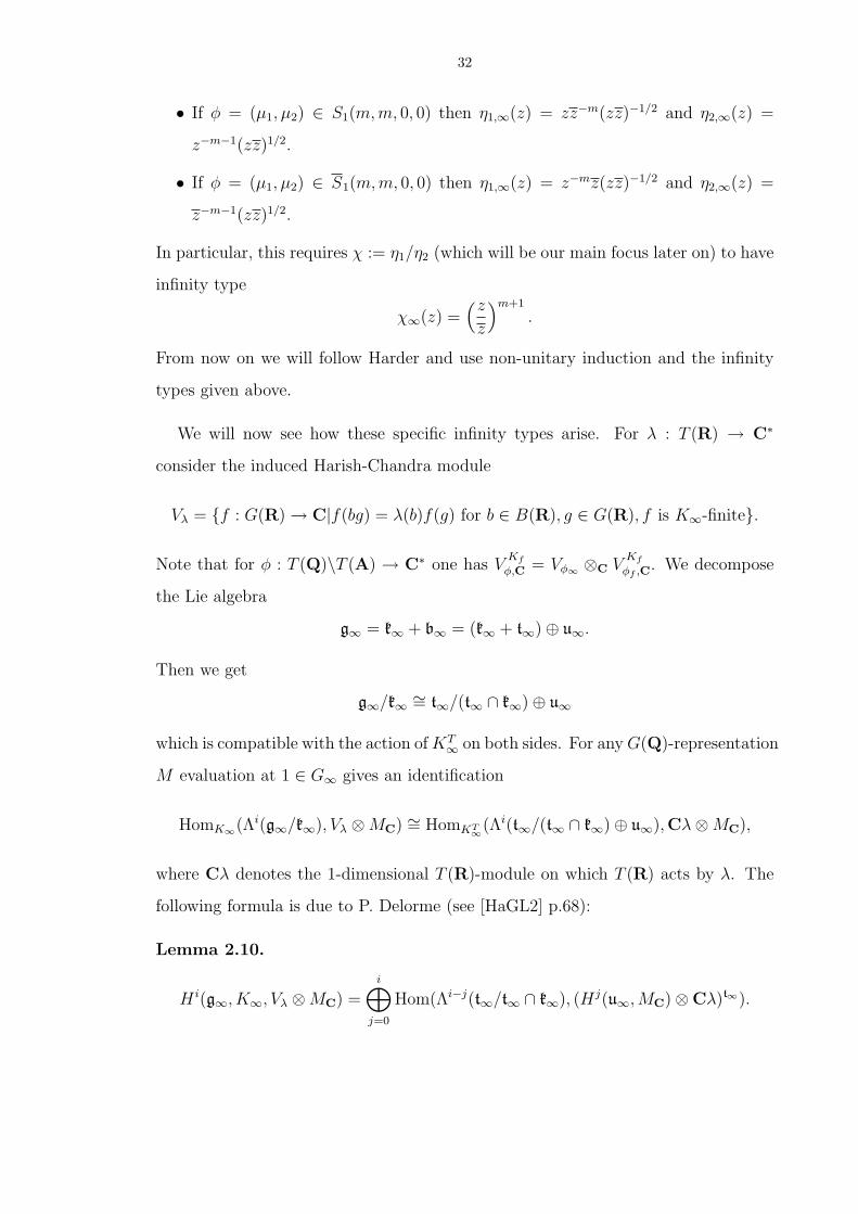
32

• If φ = (µ1, µ2) ∈ S1(m,m, 0, 0) then η1,∞(z) = zz−m(zz)−1/2 and η2,∞(z) =

z−m−1(zz)1/2.

• If φ = (µ1, µ2) ∈ S1(m,m, 0, 0) then η1,∞(z) = z−mz(zz)−1/2 and η2,∞(z) =

z−m−1(zz)1/2.

In particular, this requires χ := η1/η2 (which will be our main focus later on) to have

infinity type

χ∞(z) =(z

z

)m+1

.

From now on we will follow Harder and use non-unitary induction and the infinity

types given above.

We will now see how these specific infinity types arise. For λ : T (R) → C∗

consider the induced Harish-Chandra module

Vλ = f : G(R) → C|f(bg) = λ(b)f(g) for b ∈ B(R), g ∈ G(R), f is K∞-finite.

Note that for φ : T (Q)\T (A) → C∗ one has VKf

φ,C = Vφ∞ ⊗C VKf

φf ,C. We decompose

the Lie algebra

g∞ = k∞ + b∞ = (k∞ + t∞)⊕ u∞.

Then we get

g∞/k∞ ∼= t∞/(t∞ ∩ k∞)⊕ u∞

which is compatible with the action of KT∞ on both sides. For any G(Q)-representation

M evaluation at 1 ∈ G∞ gives an identification

HomK∞(Λi(g∞/k∞), Vλ ⊗MC) ∼= HomKT∞(Λi(t∞/(t∞ ∩ k∞)⊕ u∞),Cλ⊗MC),

where Cλ denotes the 1-dimensional T (R)-module on which T (R) acts by λ. The

following formula is due to P. Delorme (see [HaGL2] p.68):

Lemma 2.10.

H i(g∞, K∞, Vλ ⊗MC) =i⊕

j=0

Hom(Λi−j(t∞/t∞ ∩ k∞), (Hj(u∞,MC)⊗Cλ)t∞).

33

The Lie algebra cohomology groups H i(u∞,Mm,nC ) can be calculated by the fol-

lowing Lemma (cf. [HaGL2] §3.5, [F], Proof of §1.4 Satz):

Lemma 2.11. (a) By the Kunneth formula we have

H i(u∞,Mm,nC [k, l]) = H i(u⊗Q C,Mm,n

C [k, l])

∼=i⊕

j=0

(Hj(u0 ⊗F C,Mm

C [k])⊕H i−j(u0 ⊗F,σ C,Mn

C[l])).

(b)

H i(u0,Mm[k]) =

FXm if i = 0,

FY m ⊗ U∨α if i = 1,

0 otherwise,

where U∨α is a generator of Hom(u0, F ).

We can therefore find cohomology classes e(1,0) and e(0,1) generating H1(u0,MmC [k])⊗

H0(u0, Mn

C[l]) and H0(u0,MmC [k])⊗H1(u0,M

n

C[l]), respectively. They are eigenvec-

tors for the action of the torus T (R). Denoting the inverses of the eigencharacters

by λ1,0(m,n, k, l) and λ0,1(m,n, k, l) respectively, we see that they are exactly the

infinity types singled out above. By Delorme’s formula H1(g∞, K∞, Vλ ⊗ Mm,nC ) is

nontrivial for λ = λ1,0(m,n, k, l) and λ = λ0,1(m,n, k, l).

We now have the following description of the cohomology of the boundary with

complex coefficients. Recall that H1(∂SKf, Mm,n

C ) is isomorphic to

H1(∂SKf, Mm,n

C ) ∼= H∗(g∞, K∞, C∞(B(Q)\G(A)/Kf )(ω−1Mm,n

C)⊗Mm,n

C ).

For each φ : T (Q)\T (A) → C∗ in S1(m,n, 0, 0) or S1(m, n, 0, 0) let

Ξφ : H∗(g∞, K∞, VKf

φ,C⊗Mm,nC ) → H∗(g∞, K∞, C∞(B(Q)\G(A)/Kf )(ω

−1Mm,n

C)⊗Mm,n

C )

be the map induced by the embedding VKf

φ,C → C∞(B(Q)\G(A)/Kf )(ω−1Mm,n

C). These

are not injective. One can, however, show the following: For (a, b) = (1, 0) and (0, 1)

let [e(a,b)] be generators of the 1-dimensional C-vector spaces

Hom(Λ0(t∞/t∞ ∩ k∞), Ha(u0,MmC [k])⊗Hb(u0,M

n

C[l])⊗Cλa,b(m,n, k, l))

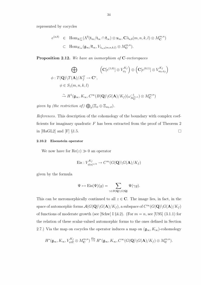
34

represented by cocycles

e(a,b) ∈ HomKT∞(Λ0(t∞/t∞ ∩ k∞)⊗ u∞,Cλa,b(m,n, k, l)⊗Mm,nC )

⊂ HomK∞(g∞/k∞, Vλa,b(m,n,k,l) ⊗Mm,nC ).

Proposition 2.12. We have an isomorphism of C-vectorspaces

⊕

φ : T (Q)\T (A)/KTf → C∗,

φ ∈ S1(m,n, k, l)

(C[e(1,0)]⊗ V

Kf

φf

)⊕

(C[e(0,1)]⊗ V

Kf

w0.φf

)

∼→ H1(g∞, K∞, C∞(B(Q)\G(A)/Kf )(ω−1Mm,n

C)⊗Mm,n

C )

given by (the restriction of)⊕

φ(Ξφ ⊕ Ξw0.φ).

References. This description of the cohomology of the boundary with complex coef-

ficients for imaginary quadratic F has been extracted from the proof of Theorem 2

in [HaGL2] and [F] §1.5.

2.10.2 Eisenstein operator

We now have for Re(z) À 0 an operator

Eis : VKf

φ|α|z/2 → C∞(G(Q)\G(A)/Kf )

given by the formula

Ψ 7→ Eis(Ψ)(g) =∑

γ∈B(Q)\G(Q)

Ψ(γg).

This can be meromorphically continued to all z ∈ C. The image lies, in fact, in the

space of automorphic formsA(G(Q)\G(A)/Kf ), a subspace of C∞(G(Q)\G(A)/Kf )

of functions of moderate growth (see [Schw] I §4.2). (For m = n, see [U95] (3.1.1) for

the relation of these scalar-valued automorphic forms to the ones defined in Section

2.7.) Via the map on cocycles the operator induces a map on (g∞, K∞)-cohomology

H∗(g∞, K∞, VKf

φ,C ⊗Mm,nC )

Eis→ H∗(g∞, K∞, C∞(G(Q)\G(A)/Kf )⊗Mm,nC ).

35

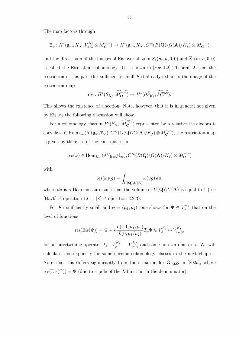
The map factors through

Ξφ : H∗(g∞, K∞, VKf

φ,C ⊗Mm,nC ) → H∗(g∞, K∞, C∞(B(Q)\G(A)/Kf )⊗Mm,n

C )

and the direct sum of the images of Eis over all φ in S1(m,n, 0, 0) and S1(m,n, 0, 0)

is called the Eisenstein cohomology. It is shown in [HaGL2] Theorem 2, that the

restriction of this part (for sufficiently small Kf ) already exhausts the image of the

restriction map

res : H∗(SKf, Mm,n

C ) → H∗(∂SKf, Mm,n

C ).

This shows the existence of a section. Note, however, that it is in general not given

by Eis, as the following discussion will show.

For a cohomology class in H i(SKf, Mm,n

C ) represented by a relative Lie algebra i-

cocycle ω ∈ HomK∞(Λi(g∞/k∞), C∞(G(Q)\G(A)/Kf )⊗Mm,nC ), the restriction map

is given by the class of the constant term

res(ω) ∈ HomK∞(Λi(g∞/k∞), C∞(B(Q)\G(A)/Kf )⊗Mm,nC )

with

res(ω)(g) =

∫

U(Q)\U(A)

ω(ug) du,

where du is a Haar measure such that the volume of U(Q)\U(A) is equal to 1 (see

[Ha79] Proposition 1.6.1, [Z] Proposition 2.2.3).

For Kf sufficiently small and φ = (µ1, µ2), one shows for Ψ ∈ VKf

φ that on the

level of functions

res(Eis(Ψ)) = Ψ + ?L(−1, µ1/µ2)

L(0, µ1/µ2)TφΨ ∈ V

Kf

φ ⊕ VKf

w0.φ,

for an intertwining operator Tφ : VKf

φ → VKf

w0.φ and some non-zero factor ?. We will

calculate this explicitly for some specific cohomology classes in the next chapter.

Note that this differs significantly from the situation for GL2,Q in [S02a], where

res(Eis(Ψ)) = Ψ (due to a pole of the L-function in the denominator).

CHAPTER III

Eisenstein cohomology

We write down an explicit Eisenstein cohomology class and calculate its constant

term and Hecke eigenvalues. We also investigate the integrality of the constant term

by translating to group cohomology.

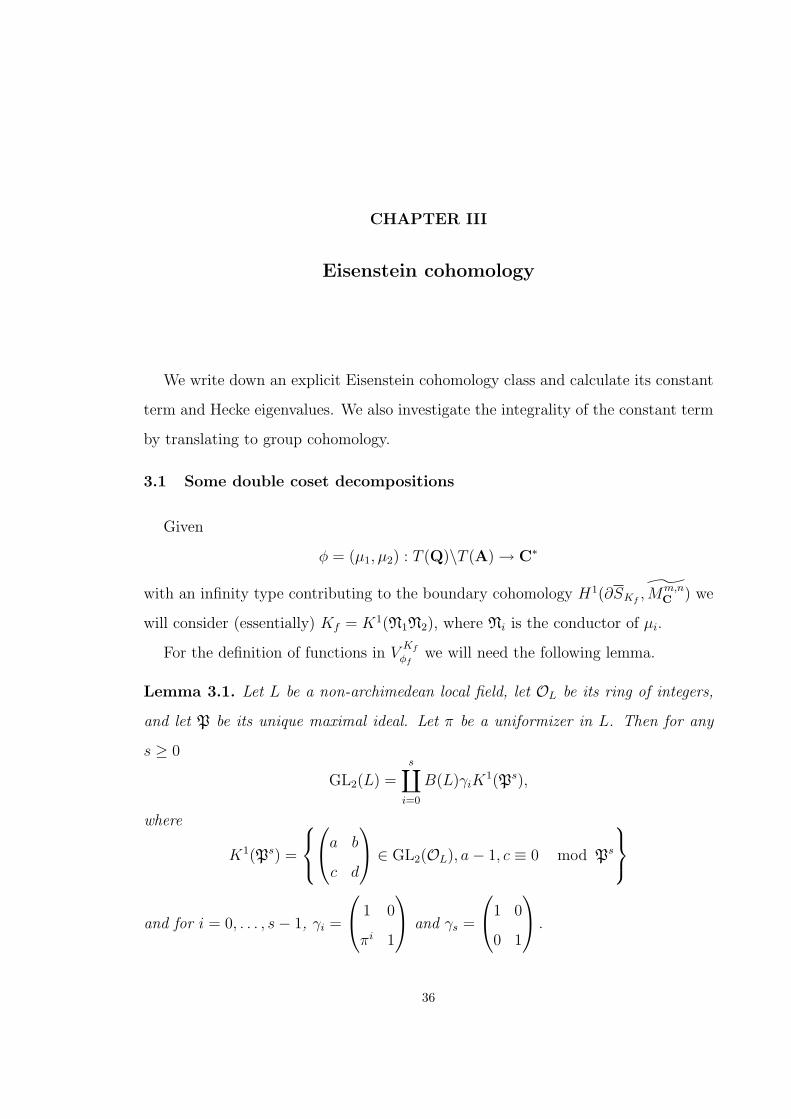
3.1 Some double coset decompositions

Given

φ = (µ1, µ2) : T (Q)\T (A) → C∗

with an infinity type contributing to the boundary cohomology H1(∂SKf, Mm,n

C ) we

will consider (essentially) Kf = K1(N1N2), where Ni is the conductor of µi.

For the definition of functions in VKf

φfwe will need the following lemma.

Lemma 3.1. Let L be a non-archimedean local field, let OL be its ring of integers,

and let P be its unique maximal ideal. Let π be a uniformizer in L. Then for any

s ≥ 0

GL2(L) =s∐

i=0

B(L)γiK1(Ps),

where

K1(Ps) =

a b

c d

∈ GL2(OL), a− 1, c ≡ 0 mod Ps

and for i = 0, . . . , s− 1, γi =

1 0

πi 1

and γs =

1 0

0 1

.

36

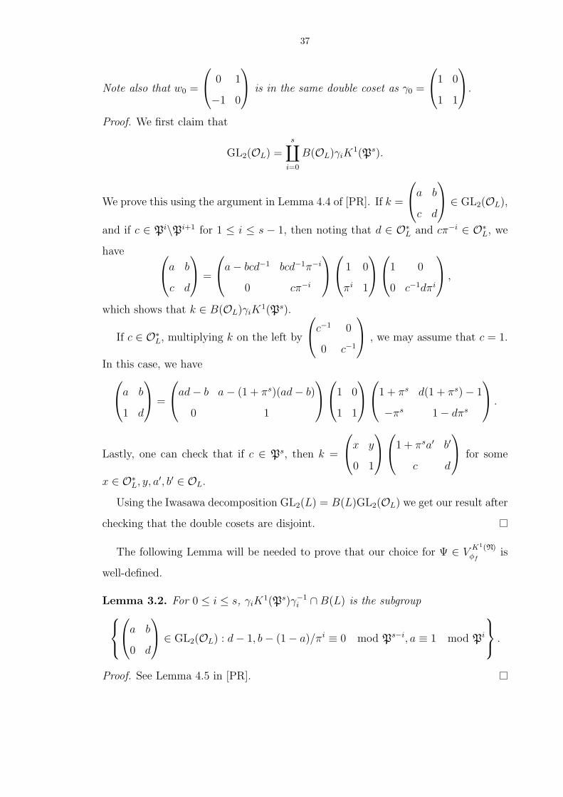
37

Note also that w0 =

0 1

−1 0

is in the same double coset as γ0 =

1 0

1 1

.

Proof. We first claim that

GL2(OL) =s∐

i=0

B(OL)γiK1(Ps).

We prove this using the argument in Lemma 4.4 of [PR]. If k =

a b

c d

∈ GL2(OL),

and if c ∈ Pi\Pi+1 for 1 ≤ i ≤ s − 1, then noting that d ∈ O∗L and cπ−i ∈ O∗

L, we

have a b

c d

=

a− bcd−1 bcd−1π−i

0 cπ−i

1 0

πi 1

1 0

0 c−1dπi

,

which shows that k ∈ B(OL)γiK1(Ps).

If c ∈ O∗L, multiplying k on the left by

c−1 0

0 c−1

, we may assume that c = 1.

In this case, we havea b

1 d

=

ad− b a− (1 + πs)(ad− b)

0 1

1 0

1 1

1 + πs d(1 + πs)− 1

−πs 1− dπs

.

Lastly, one can check that if c ∈ Ps, then k =

x y

0 1

1 + πsa′ b′

c d

for some

x ∈ O∗L, y, a′, b′ ∈ OL.

Using the Iwasawa decomposition GL2(L) = B(L)GL2(OL) we get our result after

checking that the double cosets are disjoint.

The following Lemma will be needed to prove that our choice for Ψ ∈ VK1(N)φf

is

well-defined.

Lemma 3.2. For 0 ≤ i ≤ s, γiK1(Ps)γ−1

i ∩B(L) is the subgroup

a b

0 d

∈ GL2(OL) : d− 1, b− (1− a)/πi ≡ 0 mod Ps−i, a ≡ 1 mod Pi

.

Proof. See Lemma 4.5 in [PR].

38

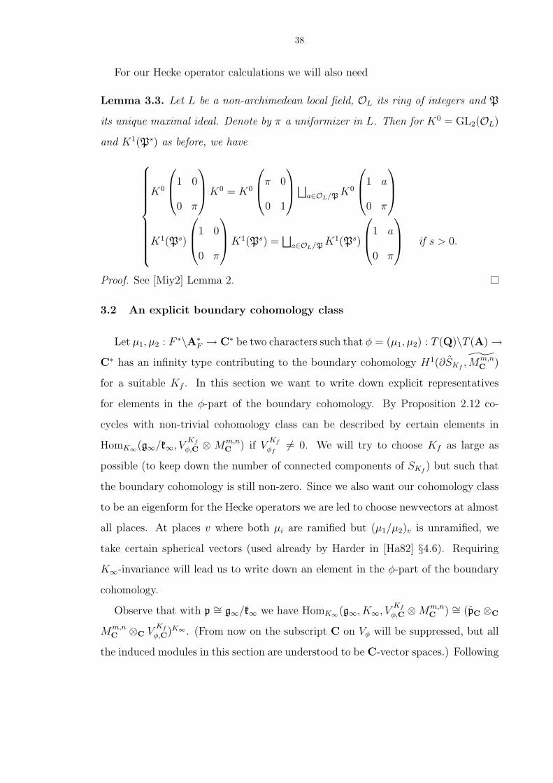
For our Hecke operator calculations we will also need

Lemma 3.3. Let L be a non-archimedean local field, OL its ring of integers and P

its unique maximal ideal. Denote by π a uniformizer in L. Then for K0 = GL2(OL)

and K1(Ps) as before, we have

K0

1 0

0 π

K0 = K0

π 0

0 1

⊔

a∈OL/P K0

1 a

0 π

K1(Ps)

1 0

0 π

K1(Ps) =

⊔a∈OL/P K1(Ps)

1 a

0 π

if s > 0.

Proof. See [Miy2] Lemma 2.

3.2 An explicit boundary cohomology class

Let µ1, µ2 : F ∗\A∗F → C∗ be two characters such that φ = (µ1, µ2) : T (Q)\T (A) →

C∗ has an infinity type contributing to the boundary cohomology H1(∂SKf, Mm,n

C )

for a suitable Kf . In this section we want to write down explicit representatives

for elements in the φ-part of the boundary cohomology. By Proposition 2.12 co-

cycles with non-trivial cohomology class can be described by certain elements in

HomK∞(g∞/k∞, VKf

φ,C ⊗ Mm,nC ) if V

Kf

φf6= 0. We will try to choose Kf as large as

possible (to keep down the number of connected components of SKf) but such that

the boundary cohomology is still non-zero. Since we also want our cohomology class

to be an eigenform for the Hecke operators we are led to choose newvectors at almost

all places. At places v where both µi are ramified but (µ1/µ2)v is unramified, we

take certain spherical vectors (used already by Harder in [Ha82] §4.6). Requiring

K∞-invariance will lead us to write down an element in the φ-part of the boundary

cohomology.

Observe that with p ∼= g∞/k∞ we have HomK∞(g∞, K∞, VKf

φ,C ⊗Mm,nC ) ∼= (pC ⊗C

Mm,nC ⊗C V

Kf

φ,C)K∞ . (From now on the subscript C on Vφ will be suppressed, but all

the induced modules in this section are understood to be C-vector spaces.) Following

39

[HaGL2] p. 80 and [Ko] p. 101 we therefore define

ωz(·, φ, Ψ) : G(A) → pC ⊗C Mm,nC

for z ∈ C and Ψ ∈ VKf

φf |α|z/2f

as

ωz(g, φ, Ψ) := ω(b∞k∞ · gf , φ|α|z/2, Ψ) =(3.1)

= (φ∞ · |α|z/2∞ )(b∞) ·Ψ(gf )

k−1∞ . (S+ ⊗ Y mX

n) if φ ∈ S1,

k−1∞ . ((−S−)⊗XmY

n) if φ ∈ S1

.

Here S1 = S1(m,n, 0, 0) and S1 = S1(m,n, 0, 0) are the two different infinity types

contributing to the boundary cohomology (cf. Section 2.10.1),

S± = 1/2

±

0 1

1 0

⊗R 1−

0 i

−i 0

⊗R i

∈ pC,

and the ‘∨’ denotes the dual vectors with respect to the killing form (see Section

2.4). The above elements of pC ⊗C Mm,nC are related to generators of H1(u∞,Mm,n

C )

as used in Proposition 2.12 under the isomorphism

u∞ ⊕CH ∼= b∞/(b∞ ∩ k∞) ∼= g∞/k∞ ∼= p∞

induced by the embedding b∞ → g∞ (cf. [Ko] §1.3.6). For the definition of VKf

φf |α|z/2f

see (2.9). One checks that if z = 0 then ω0 is a relative Lie algebra 1-cocycle (see

[Ha79] Lemma 1.5.2). We write [ω0(φ, Ψ)] both for the corresponding cohomology

class in H1(g∞, k∞, Vφ ⊗Mm,nC ) as well as its image under Ξφ in H1(∂SKf

, Mm,nC ).

Given η = (η1, η2) : T (Q)\T (A) → C∗ we now want to fix a choice of Kf and

Ψ ∈ VKfηf for which the constant term will have a particularly nice form. The function

will be denoted by Ψηf. As Kf we will take K1(M1M2) (at least away from finitely

many places), where Mi is the conductor of ηi. We will drop the subscript ηf if it is

clear what is meant from the context.

We define Ψηfas a product of local factors

∏v Ψη,v. We will also use the notation

Vηv = Ψv : G(Fv) → C | Ψ(bvgv) = ηv(bv)Ψ(gv), and denote the elements Ψη,v ∈Vηv sometimes by Ψηv .

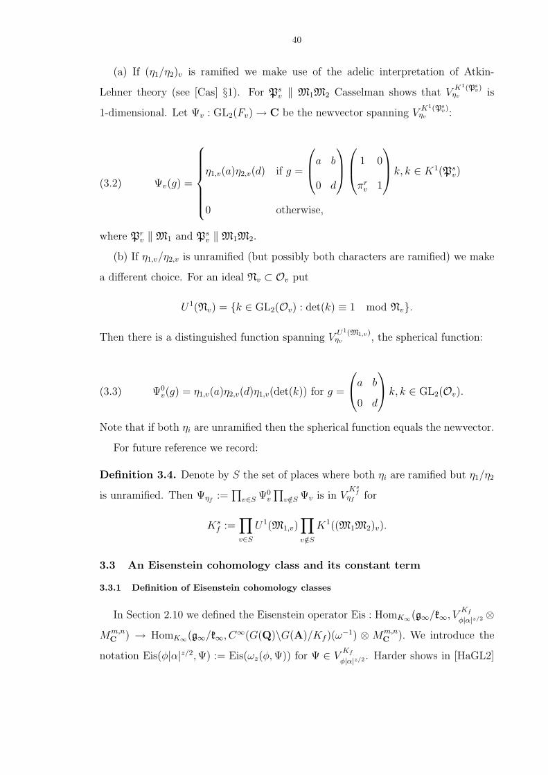
40

(a) If (η1/η2)v is ramified we make use of the adelic interpretation of Atkin-

Lehner theory (see [Cas] §1). For Psv ‖ M1M2 Casselman shows that V

K1(Psv)

ηv is

1-dimensional. Let Ψv : GL2(Fv) → C be the newvector spanning VK1(Ps

v)ηv :

(3.2) Ψv(g) =

η1,v(a)η2,v(d) if g =

a b

0 d

1 0

πrv 1

k, k ∈ K1(Ps

v)

0 otherwise,

where Prv ‖ M1 and Ps

v ‖ M1M2.

(b) If η1,v/η2,v is unramified (but possibly both characters are ramified) we make

a different choice. For an ideal Nv ⊂ Ov put

U1(Nv) = k ∈ GL2(Ov) : det(k) ≡ 1 mod Nv.

Then there is a distinguished function spanning VU1(M1,v)ηv , the spherical function:

(3.3) Ψ0v(g) = η1,v(a)η2,v(d)η1,v(det(k)) for g =

a b

0 d

k, k ∈ GL2(Ov).

Note that if both ηi are unramified then the spherical function equals the newvector.

For future reference we record:

Definition 3.4. Denote by S the set of places where both ηi are ramified but η1/η2

is unramified. Then Ψηf:=

∏v∈S Ψ0

v

∏v/∈S Ψv is in V

Ksf

ηf for

Ksf :=

∏v∈S

U1(M1,v)∏

v/∈S

K1((M1M2)v).

3.3 An Eisenstein cohomology class and its constant term

3.3.1 Definition of Eisenstein cohomology classes

In Section 2.10 we defined the Eisenstein operator Eis : HomK∞(g∞/k∞, VKf

φ|α|z/2 ⊗Mm,n

C ) → HomK∞(g∞/k∞, C∞(G(Q)\G(A)/Kf )(ω−1) ⊗ Mm,n

C ). We introduce the

notation Eis(φ|α|z/2, Ψ) := Eis(ωz(φ, Ψ)) for Ψ ∈ VKf

φ|α|z/2 . Harder shows in [HaGL2]

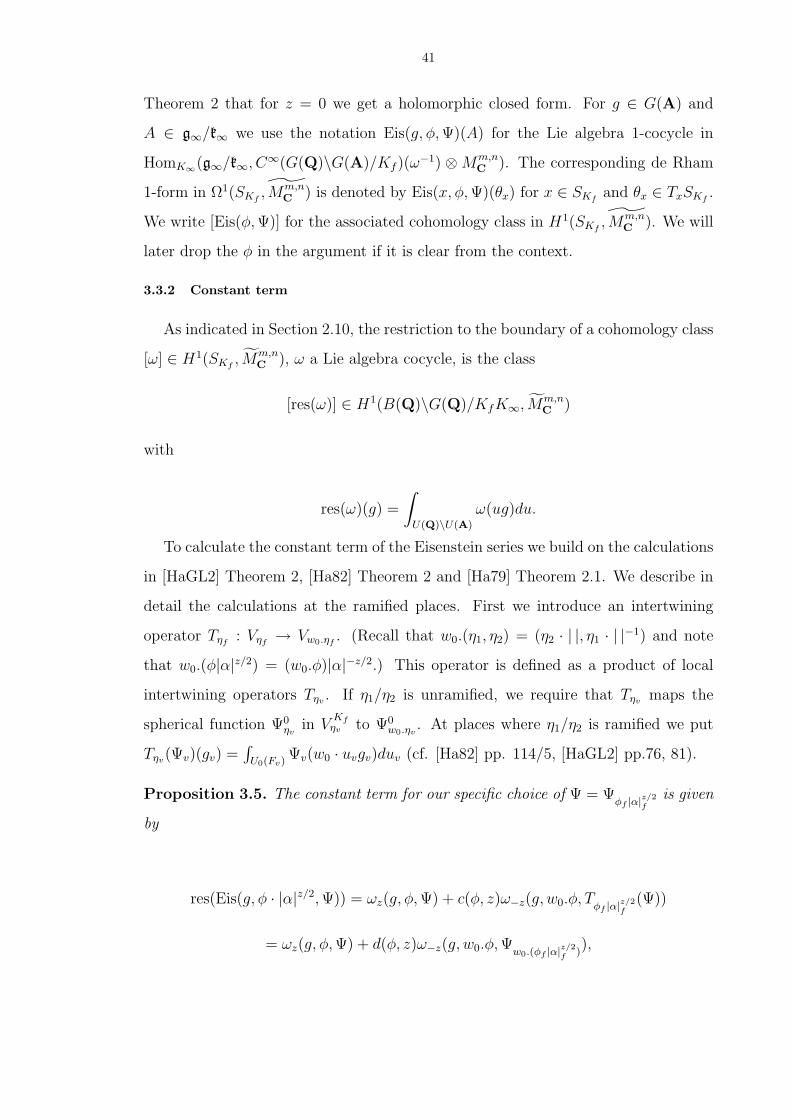
41

Theorem 2 that for z = 0 we get a holomorphic closed form. For g ∈ G(A) and

A ∈ g∞/k∞ we use the notation Eis(g, φ, Ψ)(A) for the Lie algebra 1-cocycle in

HomK∞(g∞/k∞, C∞(G(Q)\G(A)/Kf )(ω−1) ⊗Mm,n

C ). The corresponding de Rham

1-form in Ω1(SKf, Mm,n

C ) is denoted by Eis(x, φ, Ψ)(θx) for x ∈ SKfand θx ∈ TxSKf

.

We write [Eis(φ, Ψ)] for the associated cohomology class in H1(SKf, Mm,n

C ). We will

later drop the φ in the argument if it is clear from the context.

3.3.2 Constant term

As indicated in Section 2.10, the restriction to the boundary of a cohomology class

[ω] ∈ H1(SKf, Mm,n

C ), ω a Lie algebra cocycle, is the class

[res(ω)] ∈ H1(B(Q)\G(Q)/KfK∞, Mm,nC )

with

res(ω)(g) =

∫

U(Q)\U(A)

ω(ug)du.

To calculate the constant term of the Eisenstein series we build on the calculations

in [HaGL2] Theorem 2, [Ha82] Theorem 2 and [Ha79] Theorem 2.1. We describe in

detail the calculations at the ramified places. First we introduce an intertwining

operator Tηf: Vηf

→ Vw0.ηf. (Recall that w0.(η1, η2) = (η2 · | |, η1 · | |−1) and note

that w0.(φ|α|z/2) = (w0.φ)|α|−z/2.) This operator is defined as a product of local

intertwining operators Tηv . If η1/η2 is unramified, we require that Tηv maps the

spherical function Ψ0ηv

in VKfηv to Ψ0

w0.ηv. At places where η1/η2 is ramified we put

Tηv(Ψv)(gv) =∫

U0(Fv)Ψv(w0 · uvgv)duv (cf. [Ha82] pp. 114/5, [HaGL2] pp.76, 81).

Proposition 3.5. The constant term for our specific choice of Ψ = Ψφf |α|z/2

fis given

by

res(Eis(g, φ · |α|z/2, Ψ)) = ωz(g, φ, Ψ) + c(φ, z)ω−z(g, w0.φ, Tφf |α|z/2

f(Ψ))

= ωz(g, φ, Ψ) + d(φ, z)ω−z(g, w0.φ, Ψw0.(φf |α|z/2

f )),

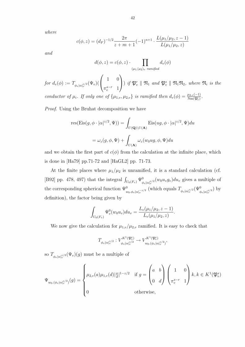
42

where

c(φ, z) = (dF )−1/2 2π

z + m + 1(−1)n+1 · L(µ1/µ2, z − 1)

L(µ1/µ2, z)

and

d(φ, z) = c(φ, z) ·∏

(µ1/µ2)v ramified

dv(φ)

for dv(φ) := Tφv |α|z/2

v(Ψv)(

1 0

πs−rv 1

) if Pr

v ‖ N1 and Psv ‖ N1N2, where Ni is the

conductor of µi. If only one of µ1,v, µ2,v is ramified then dv(φ) = µ2,v(−1)

Nm(Prv)

.

Proof. Using the Bruhat decomposition we have

res(Eis(g, φ · |α|z/2, Ψ)) =

∫

U(Q)\U(A)

Eis(ug, φ · |α|z/2, Ψ)du

= ωz(g, φ, Ψ) +

∫

U(A)

ωz(w0ug, φ, Ψ)du

and we obtain the first part of c(φ) from the calculation at the infinite place, which

is done in [Ha79] pp.71-72 and [HaGL2] pp. 71-73.

At the finite places where µ1/µ2 is unramified, it is a standard calculation (cf.

[B92] pp. 478, 497) that the integral∫

U0(Fv)Ψ0

φv |α|z/2v

(w0uvgv)duv gives a multiple of

the corresponding spherical function Ψ0

w0.φv |α|−z/2v

(which equals Tφv |α|z/2

v(Ψ0

φv |α|z/2v

) by

definition), the factor being given by

∫

U0(Fv)

Ψ0v(w0uv)duv =

Lv(µ1/µ2, z − 1)

Lv(µ1/µ2, z).

We now give the calculation for µ1,v/µ2,v ramified. It is easy to check that

Tφv |α|z/2

v: V

K1(Psv)

φv |α|z/2v

→ VK1(Ps

v)

w0.(φv |α|z/2v )

,

so Tφv |α|z/2

v(Ψv)(g) must be a multiple of

Ψw0.(φv |α|z/2

v )(g) =

µ2,v(a)µ1,v(d)|ad|1−z/2 if g =

a b

0 d

1 0

πs−rv 1

k, k ∈ K1(Ps

v)

0 otherwise,

43

the newvector spanning VK1(Ps

v)

w0.(φv |α|z/2v )

. The multiple is given by

dv(φ) = Tφv |α|z/2

v(Ψv)(

1 0

πs−rv 1

).

Next note that

Tφv |α|z/2

v(Ψv)(gv) =

∫

U0(Fv)

Ψv(w0uvgv)duv

=

∫

U0(Ov)

Ψv(w0uvgv)duv +∞∑

n=1

∫

π−nv O∗v

Ψv(w0

1 x

0 1

gv)dx.

The important cases for us are:

(I) r = 0, i.e., µ1,v is unramified, but s > 0

(II) s− r = 0, i.e., µ2,v is unramified, but r > 0

The situation for other values of r and s is messy; in certain cases dv(φ) can be zero.

We will always be able to put ourselves in the situation of Case I or II.

In Case I we have that [

1 0

πs−rv 1

] = [

1 0

0 1

] (‘[ ]’ indicating the double coset

in B(Fv)\G(Fv)/K1(Ps

v)), so we can determine dv(φ) by evaluating at the identity

matrix. The terms in the infinite sum all turn out to be zero since for n ≥ 1 and

x ∈ O∗v

w0 ·1 π−n

v x

0 1

=

−πn

v x−1 1

0 −π−nv x

1 0

πnv x−1 1

does not lie in the same double coset as

1 0

1 1

and so gets mapped to zero by Ψ.

The constant dv(φ) is therefore given by

∫

Ov

Ψ(

0 1

−1 0

1 x

0 1

)dx =

∫

Ov

Ψ(

0 1

−1 0

)dx =

vol(Ov)µ1,v(−1)µ2,v(−1) = µ2,v(−1),

where we have used that 0 1

−1 0

=

−1 1 + πs

0 −1

1 0

1 1

1 + πs −1

−πs 1

.

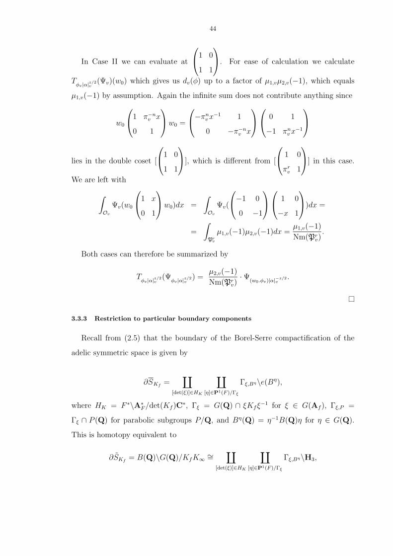
44

In Case II we can evaluate at

1 0

1 1

. For ease of calculation we calculate

Tφv |α|z/2

v(Ψv)(w0) which gives us dv(φ) up to a factor of µ1,vµ2,v(−1), which equals

µ1,v(−1) by assumption. Again the infinite sum does not contribute anything since

w0

1 π−n

v x

0 1

w0 =

−πn

v x−1 1

0 −π−nv x

0 1

−1 πnv x−1

lies in the double coset [

1 0

1 1

], which is different from [

1 0

πrv 1

] in this case.

We are left with

∫

Ov

Ψv(w0

1 x

0 1

w0)dx =

∫

Ov

Ψv(

−1 0

0 −1

1 0

−x 1

)dx =

=

∫

Prv

µ1,v(−1)µ2,v(−1)dx =µ1,v(−1)

Nm(Prv)

.

Both cases can therefore be summarized by

Tφv |α|z/2

v(Ψ

φv |α|z/2v

) =µ2,v(−1)

Nm(Prv)·Ψ

(w0.φv)|α|−z/2v

.

3.3.3 Restriction to particular boundary components

Recall from (2.5) that the boundary of the Borel-Serre compactification of the

adelic symmetric space is given by

∂SKf=

∐

[det(ξ)]∈HK

∐

[η]∈P1(F )/Γξ

Γξ,Bη\e(Bη),

where HK = F ∗\A∗F /det(Kf )C

∗, Γξ = G(Q) ∩ ξKfξ−1 for ξ ∈ G(Af ), Γξ,P =

Γξ ∩ P (Q) for parabolic subgroups P/Q, and Bη(Q) = η−1B(Q)η for η ∈ G(Q).

This is homotopy equivalent to

∂SKf= B(Q)\G(Q)/KfK∞ ∼=

∐

[det(ξ)]∈HK

∐

[η]∈P1(F )/Γξ

Γξ,Bη\H3,

45

where the boundary component Γξ,Bη\H3 gets embedded in ∂SKfvia g∞ 7→ jη,ξ(g∞) :=

η(g∞, ξ).

We will be interested in the restriction of cohomology classes to the boundary com-

ponents Γξ,P\e(P ) ∼ Γξ,P\H3. So in the next lemma we clarify the relation between

the various descriptions of the boundary restrictions of a class in H1(SKf, Mm,n

C ).

Lemma 3.6 (Definition/Lemma). (a) For [ω] ∈ H1(∂SKf, Mm,n

C ), ω a Lie algebra

cocycle, the restriction to H1(Γξ,P\H3, Mm,nC ) is given by the class of ωξ

P := j∗η,ξ(ω)

if P = Bη.

(b) For [ω] ∈ H1(SKf, Mm,n

C ), ω a Lie algebra cocycle, the restriction to

H1(Γξ,P\H3, Mm,nC )

is given by the class of

resξP (ω)(g) =

∫

UP (Q)\UP (A)

ω(ugξ)du

for g ∈ G∞, where UP is the nilpotent part of the parabolic P . We have resξP (ω) =

(res(ω))ξP , where res(ω) is the constant term defined in section 2.10.

Remark 3.7. The “constant term of ω with respect to P” is given by

∫

UP (Q)\UP (A)

ω(ug)du.

Since we will not be using this general notion, “constant term” will always refer to

the one with respect to B, as defined in Section 2.10.

Proof. If one takes for granted the statements about the constant term recalled in

Section 2.10 and the comments at the start of this section on the embedding of

the boundary component, then the restriction to Γξ,P for P = Bη is given by

res(ω)(jη,ξ(g)) =∫

U(Q)\U(A)ω(uηgξ)du. The latter equals

∫UP (Q)\UP (A)

ω(ugξ)du since

ω is invariant under multiplication by η−1 on the left.

Alternatively, one can refer to Proposition 2.2.3 of [Z] which proves that the

restriction of [ω]|jξ(Γξ\H3) to the boundary component Γξ,P\H3 is given by the class

46

of ∫

Γξ,UP\UP (R)

ω(u∞gξ)du∞.

Strong approximation for UP (A) shows that this agrees with the expression given

above.

3.3.4 Translation to group cohomology

By Proposition 2.5 the de Rham cohomology group H1(Γξ,P\H3, N) is naturally

isomorphic to the cohomology group H1(Γξ,P , N) for any C[Γξ,P ]-module N . After

a choice of basepoint x0 ∈ H3 this isomorphism is given by mapping a closed 1-form

ω with values in N to the following 1-cocyle:

Gx0(ω) : γ 7→∫ γ.x0

x0

ω.

For later considerations it will be convenient to translate the restrictions ωξP of

adelic boundary cohomology classes ω to group cohomology for the arithmetic sub-

groups Γξ,P , i.e. to make the isomorphism

(3.4) H1(∂SKf, MC) ∼=

⊕

[det(ξ)]∈HK

⊕

[η]∈P1(F )/Γξ

H1(Γξ,Bη , Mξ ⊗C)

(cf. Section 2.9.2) explicit for M an O[16, G(Q)]-module. Note that Mξ ⊗ C = MC.

To combine this with the results of the previous section on the restriction of Lie

algebra cohomology classes to a boundary component, recall from Section 2.9.3 how

to translate a Lie algebra cocycle ω ∈ HomK∞(g∞/k∞, C∞(Γ\GL2(C))(ω−1∞ )⊗MC)

to a closed 1-form ω: Reversing the isomorphism given there, for x∞ = g∞K∞ ∈ H3

and T ∈ Tx∞H3 let

ω(x∞)(T ) := g∞.ω(g∞)(DL−1g∞

T ).

For a particular choice of basepoint we then get a fairly nice expression for the

image of a boundary cohomology class in H1(∂SKf, Mm,n

C ) (represented by a relative

Lie algebra 1-cocycle ω) in the group cohomology of Γξ,P :

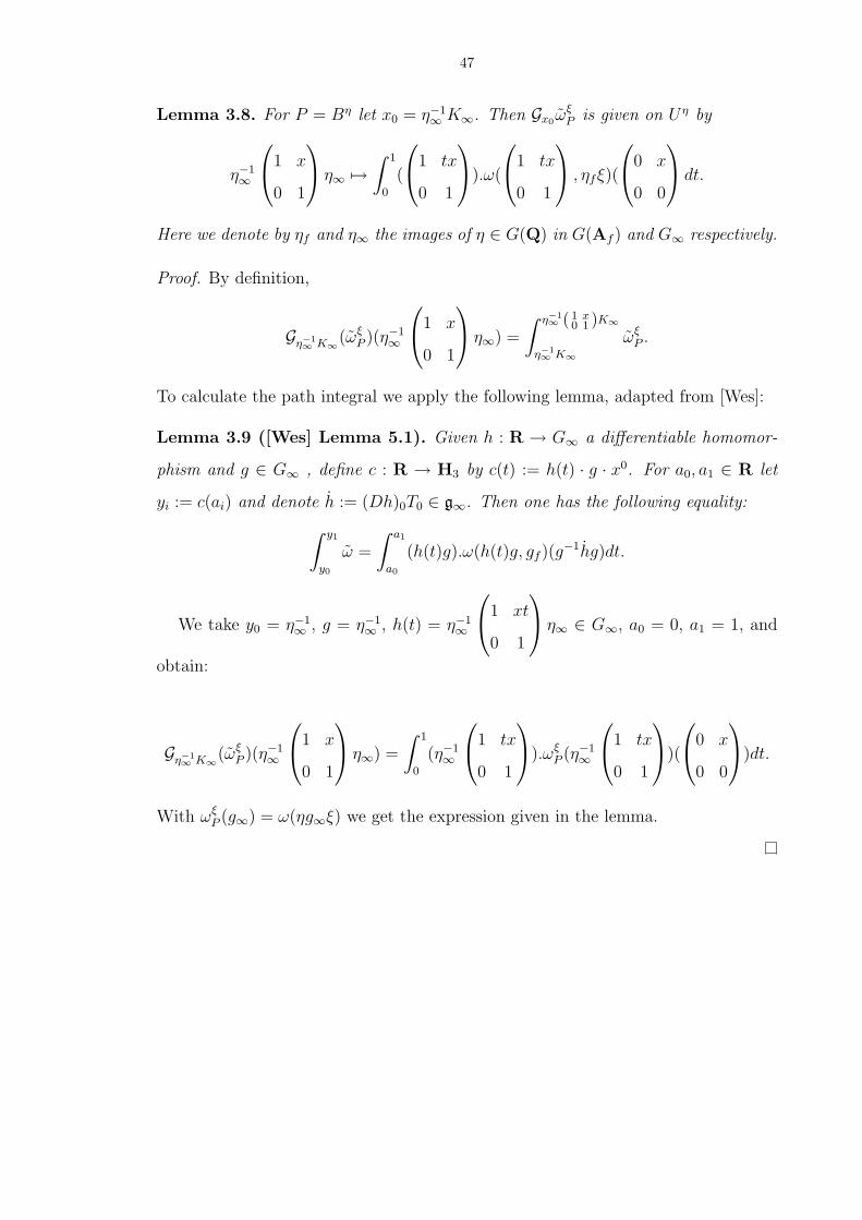
47

Lemma 3.8. For P = Bη let x0 = η−1∞ K∞. Then Gx0ω

ξP is given on Uη by

η−1∞

1 x

0 1

η∞ 7→

∫ 1

0

(

1 tx

0 1

).ω(

1 tx

0 1

, ηfξ)(

0 x

0 0

dt.

Here we denote by ηf and η∞ the images of η ∈ G(Q) in G(Af ) and G∞ respectively.

Proof. By definition,

Gη−1∞ K∞(ωξP )(η−1

∞

1 x

0 1

η∞) =

∫ η−1∞ ( 1 x0 1 )K∞

η−1∞ K∞ωξ

P .

To calculate the path integral we apply the following lemma, adapted from [Wes]:

Lemma 3.9 ([Wes] Lemma 5.1). Given h : R → G∞ a differentiable homomor-

phism and g ∈ G∞ , define c : R → H3 by c(t) := h(t) · g · x0. For a0, a1 ∈ R let

yi := c(ai) and denote h := (Dh)0T0 ∈ g∞. Then one has the following equality:

∫ y1

y0

ω =

∫ a1

a0

(h(t)g).ω(h(t)g, gf )(g−1hg)dt.

We take y0 = η−1∞ , g = η−1

∞ , h(t) = η−1∞

1 xt

0 1

η∞ ∈ G∞, a0 = 0, a1 = 1, and

obtain:

Gη−1∞ K∞(ωξP )(η−1

∞

1 x

0 1

η∞) =

∫ 1

0

(η−1∞

1 tx

0 1

).ωξ

P (η−1∞

1 tx

0 1

)(

0 x

0 0

)dt.

With ωξP (g∞) = ω(ηg∞ξ) we get the expression given in the lemma.

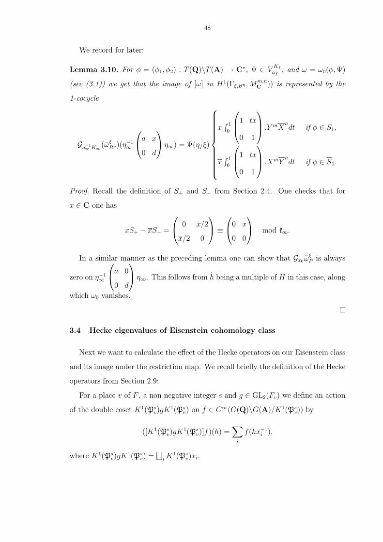
48

We record for later:

Lemma 3.10. For φ = (φ1, φ2) : T (Q)\T (A) → C∗, Ψ ∈ VKf

φf, and ω = ω0(φ, Ψ)

(see (3.1)) we get that the image of [ω] in H1(Γξ,Bη ,Mm,nC )) is represented by the

1-cocycle

Gη−1∞ K∞(ωξBη)(η−1

∞

a x

0 d

η∞) = Ψ(ηfξ)

x∫ 1

0

1 tx

0 1

.Y mX

ndt if φ ∈ S1,

x∫ 1

0

1 tx

0 1

.XmY

ndt if φ ∈ S1.

Proof. Recall the definition of S+ and S− from Section 2.4. One checks that for

x ∈ C one has

xS+ − xS− =

0 x/2

x/2 0

≡

0 x

0 0

mod k∞.

In a similar manner as the preceding lemma one can show that Gx0ωξP is always

zero on η−1∞

a 0

0 d

η∞. This follows from h being a multiple of H in this case, along

which ω0 vanishes.

3.4 Hecke eigenvalues of Eisenstein cohomology class

Next we want to calculate the effect of the Hecke operators on our Eisenstein class

and its image under the restriction map. We recall briefly the definition of the Hecke

operators from Section 2.9:

For a place v of F , a non-negative integer s and g ∈ GL2(Fv) we define an action

of the double coset K1(Psv)gK1(Ps

v) on f ∈ C∞(G(Q)\G(A)/K1(Psv)) by

([K1(Psv)gK1(Ps

v)]f)(h) =∑

i

f(hx−1i ),

where K1(Psv)gK1(Ps

v) =⊔

i K1(Ps

v)xi.

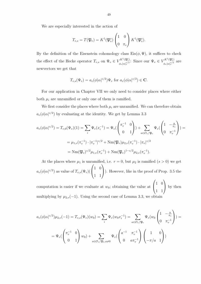
49

We are especially interested in the action of

Tv,s = T (Pv) = K1(Psv)

1 0

0 πv

K1(Ps

v).

By the definition of the Eisenstein cohomology class Eis(φ, Ψ), it suffices to check

the effect of the Hecke operator Tv,s on Ψv ∈ VK1(Ps

v)

φv |α|z/2v

: Since our Ψv ∈ VK1(Ps

v)

φv |α|z/2v

are

newvectors we get that

Tv,s(Ψv) = av(φ|α|z/2)Ψv for av(φ|α|z/2) ∈ C.

For our application in Chapter VII we only need to consider places where either

both µi are unramified or only one of them is ramified.

We first consider the places where both µi are unramified. We can therefore obtain

av(φ|α|z/2) by evaluating at the identity. We get by Lemma 3.3

av(φ|α|z/2) = Tv,0(Ψv)(1) =∑

i

Ψv(x−1i ) = Ψv(

π−1

v 0

0 1

) +

∑

a∈Ov/Pv

Ψv(

1 − a

πv

0 π−1v

) =

= µ1,v(π−1v ) · |π−1

v |z/2 + Nm(Pv)µ2,v(π−1v ) · |πv|z/2

= Nm(Pv)z/2µ1,v(π

−1v ) + Nm(Pv)

1−z/2µ2,v(π−1v ).

At the places where µ1 is unramified, i.e. r = 0, but µ2 is ramified (s > 0) we get

av(φ|α|z/2) as value of Tv,s(Ψv)(

1 0

1 1

). However, like in the proof of Prop. 3.5 the

computation is easier if we evaluate at w0; obtaining the value at

1 0

1 1

by then

multiplying by µ2,v(−1). Using the second case of Lemma 3.3, we obtain

av(φ|α|z/2)µ2,v(−1) = Tv,s(Ψv)(w0) =∑

i

Ψv(w0x−1i ) =

∑

a∈Ov/Pv

Ψv(w0

1 − a

πv

0 π−1v

) =

= Ψv(

π−1

v 0

0 1

w0) +

∑

a∈Ov/Pv ,a6=0

Ψv(

a−1 π−1

v

0 aπ−1v

1 0

−π/a 1

)

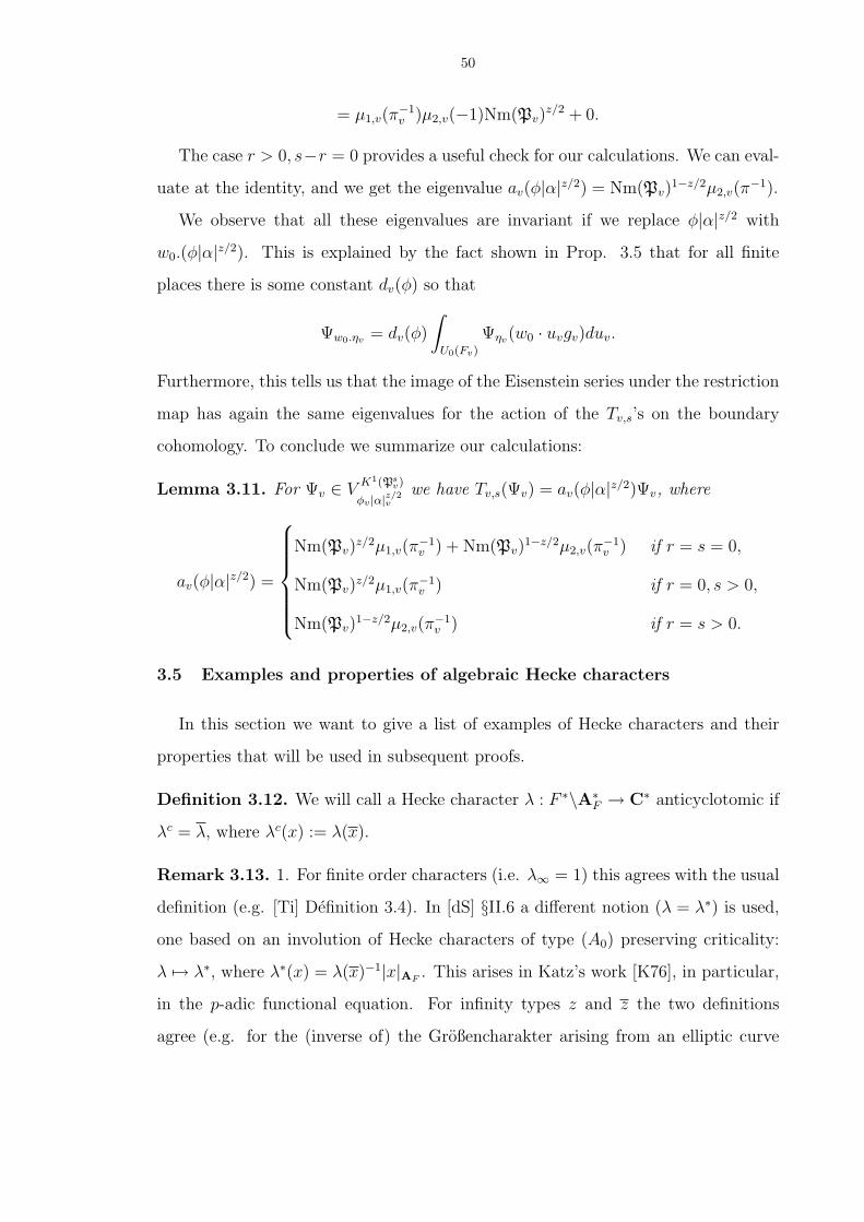
50

= µ1,v(π−1v )µ2,v(−1)Nm(Pv)

z/2 + 0.

The case r > 0, s−r = 0 provides a useful check for our calculations. We can eval-

uate at the identity, and we get the eigenvalue av(φ|α|z/2) = Nm(Pv)1−z/2µ2,v(π

−1).

We observe that all these eigenvalues are invariant if we replace φ|α|z/2 with

w0.(φ|α|z/2). This is explained by the fact shown in Prop. 3.5 that for all finite

places there is some constant dv(φ) so that

Ψw0.ηv = dv(φ)

∫

U0(Fv)

Ψηv(w0 · uvgv)duv.

Furthermore, this tells us that the image of the Eisenstein series under the restriction

map has again the same eigenvalues for the action of the Tv,s’s on the boundary

cohomology. To conclude we summarize our calculations:

Lemma 3.11. For Ψv ∈ VK1(Ps

v)

φv |α|z/2v

we have Tv,s(Ψv) = av(φ|α|z/2)Ψv, where

av(φ|α|z/2) =

Nm(Pv)z/2µ1,v(π

−1v ) + Nm(Pv)

1−z/2µ2,v(π−1v ) if r = s = 0,

Nm(Pv)z/2µ1,v(π

−1v ) if r = 0, s > 0,

Nm(Pv)1−z/2µ2,v(π

−1v ) if r = s > 0.

3.5 Examples and properties of algebraic Hecke characters

In this section we want to give a list of examples of Hecke characters and their

properties that will be used in subsequent proofs.

Definition 3.12. We will call a Hecke character λ : F ∗\A∗F → C∗ anticyclotomic if

λc = λ, where λc(x) := λ(x).

Remark 3.13. 1. For finite order characters (i.e. λ∞ = 1) this agrees with the usual

definition (e.g. [Ti] Definition 3.4). In [dS] §II.6 a different notion (λ = λ∗) is used,

one based on an involution of Hecke characters of type (A0) preserving criticality:

λ 7→ λ∗, where λ∗(x) = λ(x)−1|x|AF. This arises in Katz’s work [K76], in particular,

in the p-adic functional equation. For infinity types z and z the two definitions

agree (e.g. for the (inverse of) the Großencharakter arising from an elliptic curve

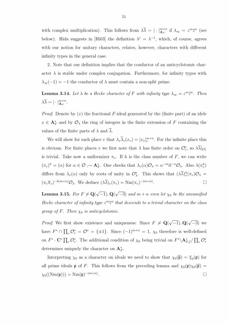
51

with complex multiplication). This follows from λλ = | · |m+nAF

if λ∞ = zmzn (see

below). Hida suggests in [Hi03] the definition λc = λ−1, which, of course, agrees

with our notion for unitary characters, relates, however, characters with different

infinity types in the general case.

2. Note that our definition implies that the conductor of an anticyclotomic char-

acter λ is stable under complex conjugation. Furthermore, for infinity types with

λ∞(−1) = −1 the conductor of λ must contain a non-split prime.

Lemma 3.14. Let λ be a Hecke character of F with infinity type λ∞ = zmzn. Then

λλ = | · |m+nAF

.

Proof. Denote by (x) the fractional F -ideal generated by the (finite part) of an idele

x ∈ A∗F and by Oλ the ring of integers in the finite extension of F containing the

values of the finite parts of λ and λ.

We will show for each place v that λvλv(xv) = |xv|m+nv . For the infinite place this

is obvious. For finite places v we first note that λ has finite order on O∗v, so λλ|O∗v

is trivial. Take now a uniformizer πv. If h is the class number of F , we can write

(πv)h = (α) for α ∈ O → A∗

F . One checks that λv(α)Oλ = α−mα−nOλ. Also λ(πhv )

differs from λv(α) only by roots of unity in O∗λ. This shows that (λλ)h

v(πv)Oλ =

(πvπv)−h(m+n)Oλ. We deduce (λλ)v(πv) = Nm(πv)

−(m+n).

Lemma 3.15. For F 6= Q(√−1),Q(

√−3) and m + n even let χ0 be the unramified

Hecke character of infinity type zmzn that descends to a trivial character on the class

group of F . Then χ0 is anticyclotomic.

Proof. We first show existence and uniqueness: Since F 6= Q(√−1),Q(

√−3) we

have F ∗ ∩ ∏v O∗

v = O∗ = ±1. Since (−1)m+n = 1, χ0 therefore is well-defined

on F ∗ · C∗ ∏v O∗

v. The additional condition of χ0 being trivial on F ∗\A∗F,f/

∏v O∗

v

determines uniquely the character on A∗F .

Interpreting χ0 as a character on ideals we need to show that χ0(p) = χ0(p) for

all prime ideals p of F . This follows from the preceding lemma and χ0(p)χ0(p) =

χ0((Nm(p))) = Nm(p)−(m+n).

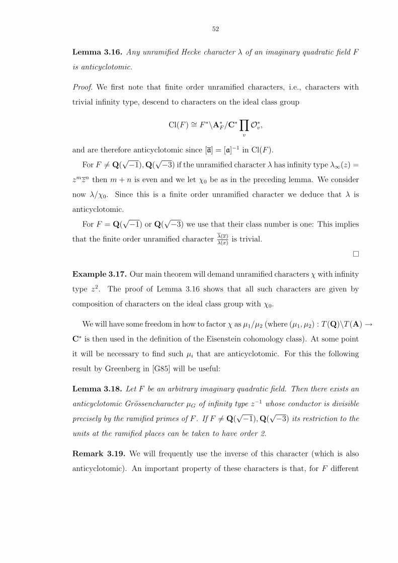
52

Lemma 3.16. Any unramified Hecke character λ of an imaginary quadratic field F

is anticyclotomic.

Proof. We first note that finite order unramified characters, i.e., characters with

trivial infinity type, descend to characters on the ideal class group

Cl(F ) ∼= F ∗\A∗F /C∗ ∏

v

O∗v,

and are therefore anticyclotomic since [a] = [a]−1 in Cl(F ).

For F 6= Q(√−1),Q(

√−3) if the unramified character λ has infinity type λ∞(z) =

zmzn then m + n is even and we let χ0 be as in the preceding lemma. We consider

now λ/χ0. Since this is a finite order unramified character we deduce that λ is

anticyclotomic.

For F = Q(√−1) or Q(

√−3) we use that their class number is one: This implies

that the finite order unramified character λ(x)λ(x)

is trivial.

Example 3.17. Our main theorem will demand unramified characters χ with infinity

type z2. The proof of Lemma 3.16 shows that all such characters are given by

composition of characters on the ideal class group with χ0.

We will have some freedom in how to factor χ as µ1/µ2 (where (µ1, µ2) : T (Q)\T (A) →C∗ is then used in the definition of the Eisenstein cohomology class). At some point

it will be necessary to find such µi that are anticyclotomic. For this the following

result by Greenberg in [G85] will be useful:

Lemma 3.18. Let F be an arbitrary imaginary quadratic field. Then there exists an

anticyclotomic Grossencharacter µG of infinity type z−1 whose conductor is divisible

precisely by the ramified primes of F . If F 6= Q(√−1),Q(

√−3) its restriction to the

units at the ramified places can be taken to have order 2.

Remark 3.19. We will frequently use the inverse of this character (which is also

anticyclotomic). An important property of these characters is that, for F different

53

from Q(√−1),Q(

√−3), their conductors contain a prime with respect to which −1

and 1 are non-congruent (i.e., some prime with residue characteristic p ≥ 3).

Proof. For Q(√−1) and Q(

√−3) Greenberg takes the Großencharaktere associated

to specific elliptic curves. In the other cases he uses the same method of construction

as in Lemma 3.15 (i.e., extension to A∗F from F ∗ ∏

v O∗vC

∗). At the ramified places

v the character is defined to be trivial on the local norm of the units (viewed as a

subgroup of O∗v). We refer to [G85] for the proof, especially that this character is

anticyclotomic.

The following character will be useful because of its minimal ramification (see also

[Ti] Lemme 2.5):

Lemma 3.20. Let ` ≥ 5 be a rational prime and l a prime of F dividing `. Then

there exists a Hecke character µl with conductor l of infinity type z.

Proof. Since ` ≥ 5, l separates the roots of unity and so the character is well-defined

on F ∗ · C∗U(l). Since the ray class group F ∗\A∗F,f/U(l) is finite we can trivially

extend to a continuous character on A∗F .

We will be using the following properties of the values of algebraic Hecke charac-

ters: Suppose p is a prime in the imaginary quadratic field F . Denote the underlying

rational prime by p.

Lemma 3.21. For µ : F ∗\A∗F → C∗ with infinity type zazb for a, b ∈ Z we let Oµ

denote the ring of integers in the finite extension Fµ of Fp obtained by adjoining the

values of the finite part of µ. Denote by v0 the place corresponding to p.

(1) For x ∈ A∗F with xv0 ∈ O∗

v0and xv0 ∈ O∗

v0we have µ(x) ∈ O∗

µ.

(2) If

a ≥ 0

a ≤ 0

then

µ−1(πv0) ∈ Oµ

µ(πv0) ∈ Oµ

.

Proof. Since µ has finite order on O∗v it suffices for (1) to show that µ(πw) ∈ O∗

µ

for w 6= v0, v0. Denote the prime ideal corresponding to πw by Pw. If h is the class

54

number of F , we have Phw = (α) for α ∈ O and α ∈ O∗

v for all v 6= w. Now

1 = µ((α, α, . . .)) = µ∞(α)µw(α)∏

v 6=w

µv(α).

Since∏

v 6=w µv(α) ∈ O∗µ and µ∞(α) = αaαb ∈ O∗

v0we deduce that µw(α) ∈ O∗

µ, i.e.,

valp(µw(α)) = 0, which implies µ(πw) ∈ O∗µ.

For (2) the same argument for w = v0 shows that valp(µw(α)) = −valp(µ∞(α)).

3.6 Integrality and rationality results

Definition 3.22. Let p be a prime of Z split in the imaginary quadratic field F

and let p be one of the primes above it. Let φ = (µ1, µ2) : T (Q)\T (A) → C∗ be

a character with φ ∈ S1(m,n, 0, 0) or φ ∈ S1(m,n, 0, 0). We put χ := µ1/µ2. Let

Oχ denote the ring of integers in the finite extension Fχ of Fp obtained by adjoining

the values of the finite part of both µi and Lalg(0, χ) ∼ L(0,χ)Ω2 , where Ω is a complex

period depending only on F . (For the algebraicity and p-adic integrality of the special

L-function value see Theorem 2.1.)

Let

H1(X, MOχ) := im(H1(X, MO ⊗O Oχ) → H1(X, M ⊗F Fχ))

for X ⊂ SKf. We will need the following results:

Proposition 3.23. Assume that the conductors of µ1 and µ2 are coprime to (p).

For constant coefficient systems (i.e., the infinity type of µ1 equals z and of µ2 equals

z−1) we have

[ω0(φ, Ψφ)], [ω0(w0.φ, Ψw0.φ)] ∈ H1(∂SKsf,Oχ).

(Here Ψφ and Ψw0.φ are the functions defined in Definition 3.4.)

Proof. In Section 3.3 we made explicit the isomorphism

H1(∂SKsf, R) ∼=

⊕

[det(ξ)]∈HKs

⊕

[η]∈P1(F )/Γξ

H1(Γξ,Bη , R),

55

which is functorial for O[16]-algebras R. Here HKs := A∗

F /det(Ks)F ∗ for Ks :=

KsfK∞, Γξ = G(Q) ∩ ξKs

fξ−1, and Γξ,Bη = Γξ ∩ η−1B(Q)η. Using this description

we associated to ω0(φ, Ψφ) a group cohomology class for R = C in Lemma 3.10. We

claim that it lies in the image of the natural map from H1(Γξ,Bη ,Oχ). Analyzing

the expression in Lemma 3.10 we need to show for all η and ξ and for all matricesa x

0 d

∈ Γξ,B that xΨφ(ηfξ) and xΨw0.φ(ηfξ) lie in Oχ. One checks that it is

sufficient to prove this for a specific choice for the set of representatives ξ and η. If

we can find a set of representatives ξ and η whose p- and p-components are units

(i.e., they are elements of GL2(Op) :=∏

v|p GL2(Ov)) then the definition of Ψφ at

places away from the conductors of the µi together with Lemma 3.21 shows that

each Ψφ(ηfξ) and Ψw0.φ(ηfξ) lies in O∗χ. For ξ this can be achieved because HKs is

a generalized ideal class group. The Chebotarev density theorem implies that each

class is represented by a prime different from p and p so we can choose ξ such that its

p- and p-components equal 1. This implies, in particular, that Γξ∩G(Qp) ⊂ GL2(Op),

so x and x from above also lie in Oχ.

For finding [η] ∈ P1(F )/Γξ = B(Q)\G(Q)/Γξ with η ∈ G(Q)∩GL2(Op) we claim

that GL2(Fp) :=∏

v|p GL2(Fv) satisfies

GL2(Fp) = B0(F )GL2(Op).

The Iwasawa decomposition implies GL2(Fp) = B0(Fp)GL2(Op). By the Chinese

Remainder Theorem we get F ·∏v|pOv =∏

v|p Fv and F ∗ ·∏v|pO∗v =

∏v|p F ∗

v and so

B0(Fp) = B0(F )B0(Op).

Together these prove our claim. Applying the claim to η′ ∈ GL2(F ) one gets a

decomposition η′ = bk with b ∈ B0(F ) and k ∈ GL2(Op). Then [η′] = [k] with

k ∈ G(Q) ∩GL2(Op).

Lemma 3.24. Assume m = n = 0, that the conductors of µ1 and µ2 are coprime

to (p), and that the conductor of χ = µ1/µ2 is coprime to the discriminant of F .

56

Assume further that at each place occuring in the conductor only one of the µi is

ramified. Then we have either

[res(Eis(ω0(φ, Ψφ))] ∈ H1(∂SKsf,Oχ)

or

[res(Eis(ω0(w0.φ, Ψw0.φ))] ∈ H1(∂SKsf,Oχ).

If χc = χ (where χc(x) := χ(x)), then the two constant terms differ only by a p-adic

unit and are both integral.

Remark 3.25. Given χ with conductor coprime to (p) and the discriminant of F one

can always factor χ = µ1/µ2 with µ1 := µl for a prime l not dividing the conductor

of χ and coprime to (p), where µl is the character defined in Lemma 3.20. Then µ1

and µ2 = µl/χ satisfy the conditions in the Lemma above.

Proof. By Proposition 3.5 the first constant term in the lemma is

ω0(φ, Ψφ)− 2π√dF

· L(−1, χ)

L(0, χ)· ω0(w0.φ, Ψw0.φ)

and we put C(χ) := 2π√dF· L(−1,χ)

L(0,χ). The second constant term is

ω0(w0.φ, Ψw0.φ)− 2π√dF

· L(−1, χ−1| · |2)L(0, χ−1| · |2) · ω0(φ, Ψφ).

Applying the functional equation (see Section 2.6) and using χχ = | · |2AF(see Lemma

3.14) one checks that the second constant term equals

ω0(w0.φ, Ψw0.φ)− C(χ)−1 · ω0(φ, Ψφ).

We note that

C(χ) =2π√dF

· L(0, χ| · |−1)

L(0, χ)∼ Lalg(0, χ| · |−1)

Lalg(0, χ),

where ‘∼’ indicates equality up to the p-adic units given by the Euler factors (1 −λ(p))(1−λ∗(p)) for λ = χ and χ| · |−1. Hence C(χ) lies in Fχ by Theorem 2.1. Since

either C(χ) ∈ Oχ or C(χ)−1 ∈ Oχ, the first statement of the Lemma follows from

Proposition 3.23.

57

For the statement for anticyclotomic characters we first observe that by the func-

tional equation

C(χ) = u(χ) · L(0, χ)

L(0, χ)

for

u(χ) :=(Nm(fχ))−1/2

W (χ)

with fχ the conductor of χ and χ = χ| · |−1. If χc = χ, then L(0, χ) = L(0, χc) =

L(0, χ), so L(0,χ)L(0,χ)

= 1. It remains to check that u(χ) ∈ O∗χ. Since the conductor of χ

is coprime to p we only need to analyze the root number W (χ) (see Section 2.6 for

its definition). The Gauss sums are p-integral because fχ is coprime to p. (This uses

Lemma 3.21.) Since fχ is coprime to the discriminant (which equals Nm(D) for the

different D) we also get that the factors χ(D−1v ) of the root number lie in O∗

χ.

We want to record here that for unramified characters χ one has u(χ) = 1. This

follows from χ(D−1) = −1, which is a consequence of F being imaginary quadratic

(see [Ha79] p.73).

Proposition 3.26.

[Eis(ω0(φ, Ψφ))] ∈ H1(SKsf, Mm,n ⊗F Fχ).

References. [HaGL2] Theorem 2, Corollary 4.2.1 and [F] Satz 1.5, [S02a] Lemma

5.1(iv). The proof uses the “Multiplicity one Theorem” for automorphic forms and

Lemma 2.7 (vanishing of residual interior cohomology).

CHAPTER IV

Denominator of the Eisenstein cohomology class

For φ = (µ1, µ2) contributing to the boundary cohomology H1(∂SKf, Mm,n

C ) and

Ψ ∈ VKf

φ|α|z/2 we defined in Section 3.3, following Harder, the Eisenstein cohomology

1-form Eis(Ψ) := Eis(φf |α|z/2f , Ψ) whose cohomology class we denote by

[Eis(Ψ)] ∈ H1(SKf, Mm,n

C ).

Harder showed that this class is, in fact, Fχ-rational, i.e., lies in H1(SKf, Mm,n

Fχ) (see

Proposition 3.26). Recall the definition of Oχ and Fχ from Definition 3.22.

Definition 4.1. If OL is the ring of integers in a (local) field L, define for any

c ∈ H1(SKf, L) the denominator (ideal)

δ(c) = a ∈ OL : ac ∈ H1(SKf,OL).

(Recall that H1(SKf,OL) = im(H1(SKf

,OL) → H1(SKf, L).)

We will give a lower bound on the denominator of the Eisenstein cohomology

class by integrating Eis(Ψ) against a suitable cycle. The (relative) cycle we use is

motivated by the classical modular symbol: we integrate along the path

σ : R>0 → H3

t 7→1 0

0 t

,

58

59

or rather a sum of such paths, one for each connected component of SKf. An expla-

nation of how to interpret this relative cycle and why the integral along it provides a

lower bound on the denominator of classes vanishing at the 0- and ∞-cusps is given

in Section 4.4.

This is the most computationally involved chapter. Instead of evaluating the

integral for the Eisenstein cohomology class defined using the function Ψφ in Vφ we

introduced in Chapter III, we consider instead the class defined using the function

Ψnew ∈ Vφ given by newvectors at all places. In 4.1 we analyze how to translate

between these classes. We then calculate in 4.2 the “toroidal” integral for Eis(Ψnew),

from which the integral for a third cohomology class Eis(Ψ′′φ) easily follows. The

denominator of this last class is then related to the denominator of Eis(Ψφ).

After restricting to constant coefficients systems (i.e., the infinity type of (µ1, µ2)

is (z, z−1)) the result of the toroidal integral calculation, up to units in Oχ, is

∫

σ

Eis(Ψ′′φ) ∼

L(0, µ1)L(0, µ−12 )

L(0, χ)=

Lalg(0, µ1)Lalg(0, µ−1

2 )

Lalg(0, χ)∈ Fχ.

From this we would like to conclude that multiplication by at least Lalg(0, χ) is

necessary to make our Eisenstein cohomology class integral, i.e., so that it lies in

H1(SKf,Oχ). However, to conclude this we need to control the p-adic properties of

the numerator.

To extract Lalg(0, χ) as the bound we use results by Hida and Finis on the non-

vanishing modulo p of the L-values Lalg(0, θµ±1i ) as θ varies in an anticyclotomic

Zq-extension for q 6= p. In Section 4.3 we replace Eis(Ψ′′φ) by a “twisted” version

Eisθ(Ψ′′φ) for a finite order character θ such that a · Eisθ(Ψ′′

φ) is integral if a · Eis(Ψ′′φ)

is. Up to units the result of the toroidal integral is then

∫

σ

Eisθ(Ψ′′φ) ∼ Lalg(0, µ1θ)L

alg(0, µ−12 θ−1)

Lalg(0, χ).

By Hida and Finis there exists a character θ such that the numerator is a p-adic unit.

The interpretation in Section 4.4 of the toroidal integral as the evaluation pairing on

a relative cycle shows that the ideal generated by Lalg(0, χ) gives a lower bound on

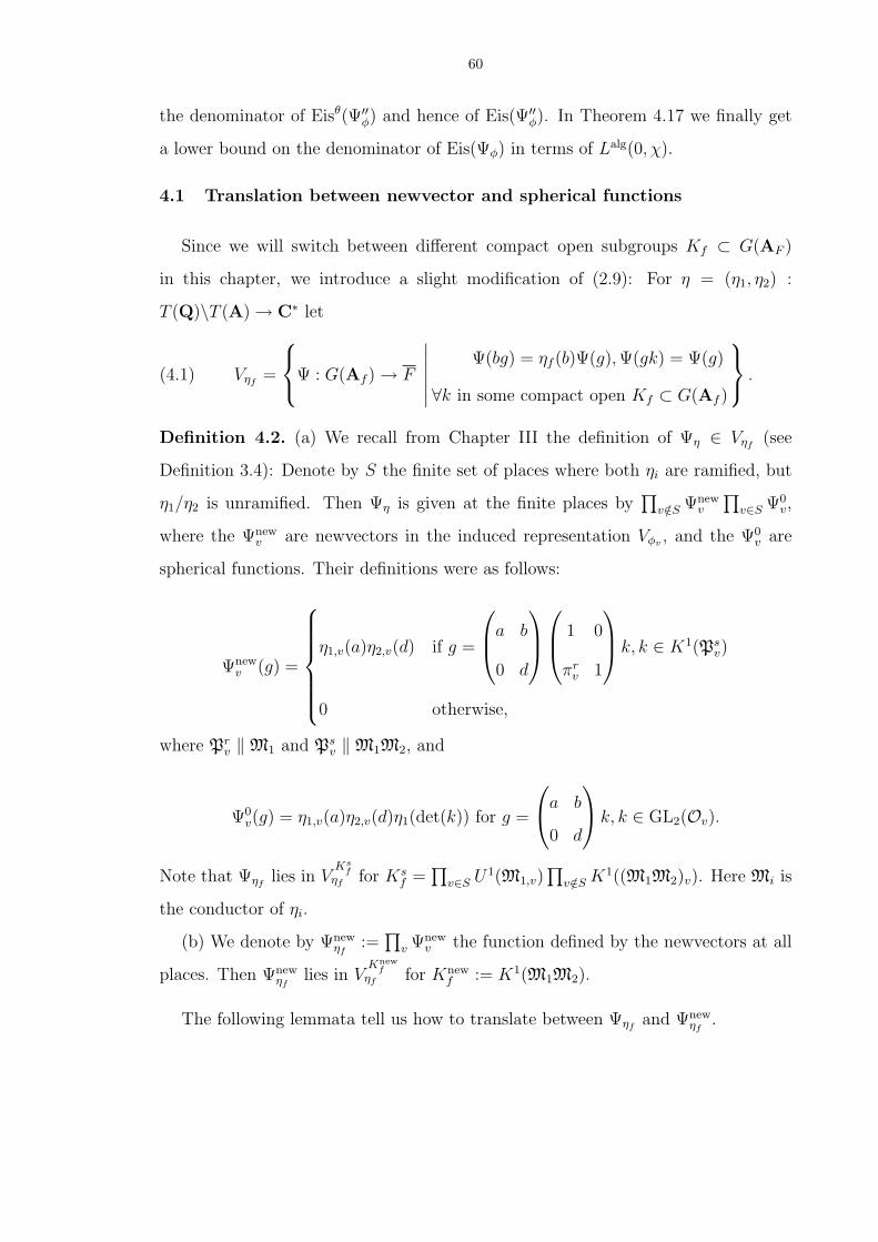
60

the denominator of Eisθ(Ψ′′φ) and hence of Eis(Ψ′′

φ). In Theorem 4.17 we finally get

a lower bound on the denominator of Eis(Ψφ) in terms of Lalg(0, χ).

4.1 Translation between newvector and spherical functions

Since we will switch between different compact open subgroups Kf ⊂ G(AF )

in this chapter, we introduce a slight modification of (2.9): For η = (η1, η2) :

T (Q)\T (A) → C∗ let

(4.1) Vηf=

Ψ : G(Af ) → F

∣∣∣∣∣∣Ψ(bg) = ηf (b)Ψ(g), Ψ(gk) = Ψ(g)

∀k in some compact open Kf ⊂ G(Af )

.

Definition 4.2. (a) We recall from Chapter III the definition of Ψη ∈ Vηf(see

Definition 3.4): Denote by S the finite set of places where both ηi are ramified, but

η1/η2 is unramified. Then Ψη is given at the finite places by∏

v/∈S Ψnewv

∏v∈S Ψ0

v,

where the Ψnewv are newvectors in the induced representation Vφv , and the Ψ0

v are

spherical functions. Their definitions were as follows:

Ψnewv (g) =

η1,v(a)η2,v(d) if g =

a b

0 d

1 0

πrv 1

k, k ∈ K1(Ps

v)

0 otherwise,

where Prv ‖ M1 and Ps

v ‖ M1M2, and

Ψ0v(g) = η1,v(a)η2,v(d)η1(det(k)) for g =

a b

0 d

k, k ∈ GL2(Ov).

Note that Ψηflies in V

Ksf

ηf for Ksf =

∏v∈S U1(M1,v)

∏v/∈S K1((M1M2)v). Here Mi is

the conductor of ηi.

(b) We denote by Ψnewηf

:=∏

v Ψnewv the function defined by the newvectors at all

places. Then Ψnewηf

lies in VKnew

fηf for Knew

f := K1(M1M2).

The following lemmata tell us how to translate between Ψηfand Ψnew

ηf.

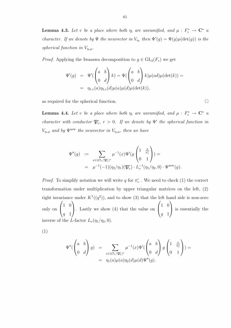
61

Lemma 4.3. Let v be a place where both ηi are unramified, and µ : F ∗v → C∗ a

character. If we denote by Ψ the newvector in Vηv then Ψ′(g) = Ψ(g)µ(det(g)) is the

spherical function in Vηvµ.

Proof. Applying the Iwasawa decomposition to g ∈ GL2(Fv) we get

Ψ′(g) = Ψ′(

a b

0 d

k) = Ψ(

a b

0 d

k)µ(ad)µ(det(k)) =

= η1,v(a)η2,v(d)µ(a)µ(d)µ(det(k)),

as required for the spherical function.

Lemma 4.4. Let v be a place where both ηi are unramified, and µ : F ∗v → C∗ a

character with conductor Prv, r > 0. If we denote by Ψ′ the spherical function in

Vηvµ and by Ψnew the newvector in Vηvµ, then we have

Ψ′′(g) :=∑

x∈(Ov/Prv)∗

µ−1(x)Ψ′(g

1 x

πrv

0 1

) =

= µ−1(−1)(η2/η1)(Prv) · L−1

v (η1/η2, 0) ·Ψnew(g).

Proof. To simplify notation we will write q for πrv . We need to check (1) the correct

transformation under multiplication by upper triangular matrices on the left, (2)

right invariance under K1((q2)), and to show (3) that the left hand side is non-zero

only on

1 0

q 1

. Lastly we show (4) that the value on

1 0

q 1

is essentially the

inverse of the L-factor Lv(η1/η2, 0).

(1)

Ψ′′(

a b

0 d

g) =

∑

x∈(Ov/Prv)∗

µ−1(x)Ψ′(

a b

0 d

g

1 x

πrv

0 1

) =

= η1(a)µ(a)η2(d)µ(d)Ψ′′(g).

62

(2) Let k =

1 + aq2 b

cq2 d

∈ K1((q2)). Now

Ψ′′(gk) =∑

x∈(Ov/Prv)∗

µ−1(x)Ψ′(g

1 + aq2 b

cq2 d

1 x

q

0 1

).

Write 1 + aq2 b

cq2 d

=

1 + aq2 0

0 d

1 b/(1 + aq2)

cq2/d 1

.

One checks that 1 b′

c′q2 1

1 x

q

0 1

=

1 x

q

0 1

1− xqc′ b′ − c′x2

q2c′ 1 + xqc′

and

a′ 0

0 d′

1 x

q

0 1

=

1 xa′

qd′

0 1

a′ 0

0 d′

.

Using Lemma 4.4 to write Ψ′(g) = Ψ(g)µ(det(g)) for the newvector Ψ in Vηv , we

obtain

Ψ′′(gk) =∑

x∈(Ov/Prv)∗

µ−1(x)Ψ(g

1 x(1+aq2)

qd

0 1

)µ(det(g))µ(d).

Now changing variable from x to x(1+aq2)qd

we get back Ψ′′(g).

(3) Let us first check that Ψ′′ is zero on

1 0

πnv 1

for n 6= r. Let

h =

1 0

πnv 1

1 x

πrv

0 1

=

1 xπ−r

v

πnv 1 + xπn−r

v

.

In the case n > r, so 1 + xπn−rv ∈ O∗

v, we have

h =

11+xπn−r

vxπ−r

v

0 1 + xπn−rv

1 0

πnv

1+xπn−rv

1

,

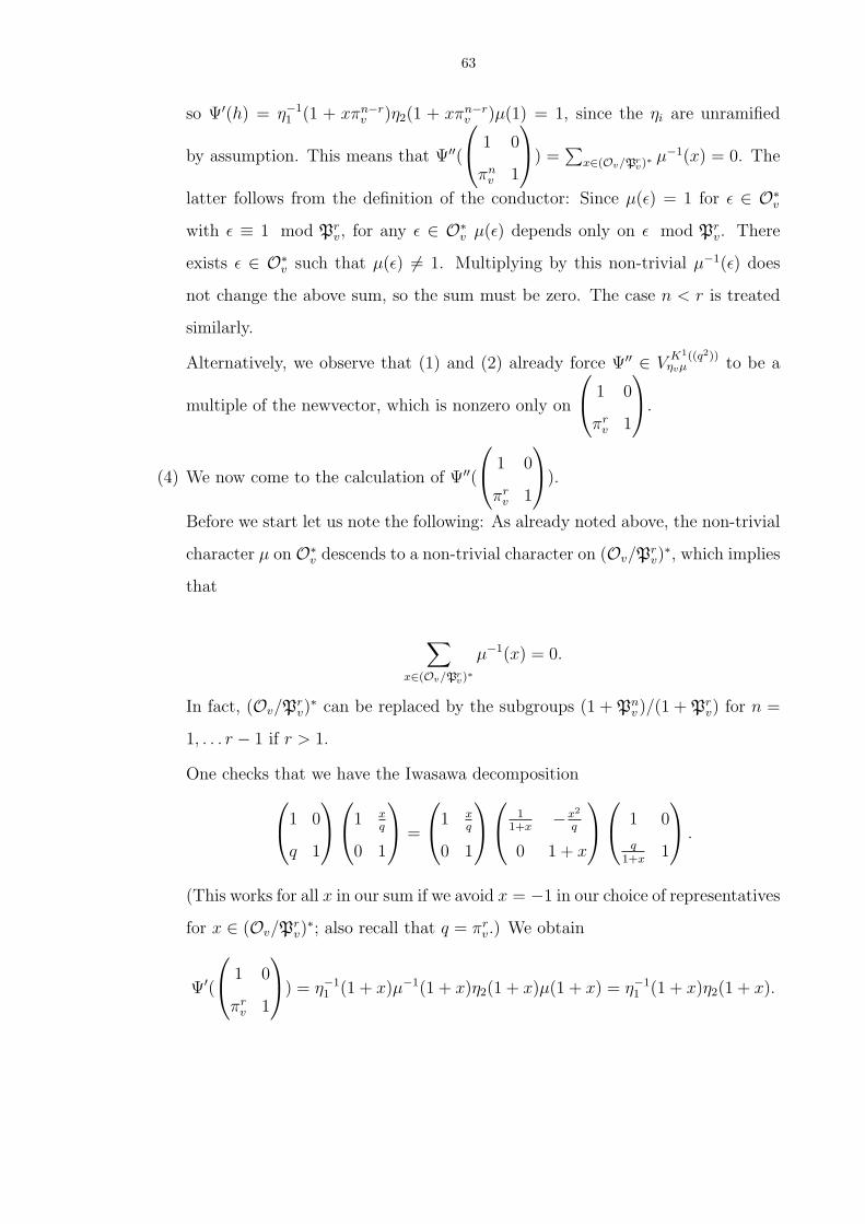
63

so Ψ′(h) = η−11 (1 + xπn−r

v )η2(1 + xπn−rv )µ(1) = 1, since the ηi are unramified

by assumption. This means that Ψ′′(

1 0

πnv 1

) =

∑x∈(Ov/Pr

v)∗ µ−1(x) = 0. The

latter follows from the definition of the conductor: Since µ(ε) = 1 for ε ∈ O∗v

with ε ≡ 1 mod Prv, for any ε ∈ O∗

v µ(ε) depends only on ε mod Prv. There

exists ε ∈ O∗v such that µ(ε) 6= 1. Multiplying by this non-trivial µ−1(ε) does

not change the above sum, so the sum must be zero. The case n < r is treated

similarly.

Alternatively, we observe that (1) and (2) already force Ψ′′ ∈ VK1((q2))ηvµ to be a

multiple of the newvector, which is nonzero only on

1 0

πrv 1

.

(4) We now come to the calculation of Ψ′′(

1 0

πrv 1

).

Before we start let us note the following: As already noted above, the non-trivial

character µ on O∗v descends to a non-trivial character on (Ov/P

rv)∗, which implies

that

∑

x∈(Ov/Prv)∗

µ−1(x) = 0.

In fact, (Ov/Prv)∗ can be replaced by the subgroups (1 + Pn

v )/(1 + Prv) for n =

1, . . . r − 1 if r > 1.

One checks that we have the Iwasawa decomposition

1 0

q 1

1 x

q

0 1

=

1 x

q

0 1

11+x

−x2

q

0 1 + x

1 0

q1+x

1

.

(This works for all x in our sum if we avoid x = −1 in our choice of representatives

for x ∈ (Ov/Prv)∗; also recall that q = πr

v.) We obtain

Ψ′(

1 0

πrv 1

) = η−1

1 (1 + x)µ−1(1 + x)η2(1 + x)µ(1 + x) = η−11 (1 + x)η2(1 + x).

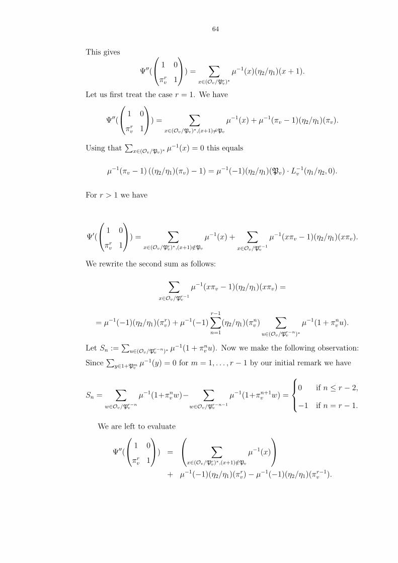
64

This gives

Ψ′′(

1 0

πrv 1

) =

∑

x∈(Ov/Prv)∗

µ−1(x)(η2/η1)(x + 1).

Let us first treat the case r = 1. We have

Ψ′′(

1 0

πrv 1

) =

∑

x∈(Ov/Pv)∗,(x+1)6=Pv

µ−1(x) + µ−1(πv − 1)(η2/η1)(πv).

Using that∑

x∈(Ov/Pv)∗ µ−1(x) = 0 this equals

µ−1(πv − 1) ((η2/η1)(πv)− 1) = µ−1(−1)(η2/η1)(Pv) · L−1v (η1/η2, 0).

For r > 1 we have

Ψ′(

1 0

πrv 1

) =

∑

x∈(Ov/Prv)∗,(x+1)/∈Pv

µ−1(x) +∑

x∈Ov/Pr−1v

µ−1(xπv − 1)(η2/η1)(xπv).

We rewrite the second sum as follows:

∑

x∈Ov/Pr−1v

µ−1(xπv − 1)(η2/η1)(xπv) =

= µ−1(−1)(η2/η1)(πrv) + µ−1(−1)

r−1∑n=1

(η2/η1)(πnv )

∑

u∈(Ov/Pr−nv )∗

µ−1(1 + πnv u).

Let Sn :=∑

u∈(Ov/Pr−nv )∗ µ−1(1 + πn

v u). Now we make the following observation:

Since∑

y∈1+Pmv

µ−1(y) = 0 for m = 1, . . . , r − 1 by our initial remark we have

Sn =∑

w∈Ov/Pr−nv

µ−1(1+πnv w)−

∑

w∈Ov/Pr−n−1v

µ−1(1+πn+1v w) =

0 if n ≤ r − 2,

−1 if n = r − 1.

We are left to evaluate

Ψ′′(

1 0

πrv 1

) =

∑

x∈(Ov/Prv)∗,(x+1)/∈Pv

µ−1(x)

+ µ−1(−1)(η2/η1)(πrv)− µ−1(−1)(η2/η1)(π

r−1v ).

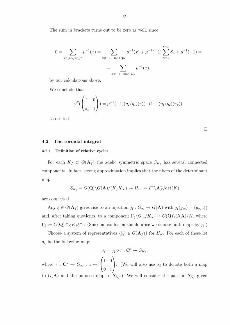
65

The sum in brackets turns out to be zero as well, since

0 =∑

x∈(Ov/Prv)∗

µ−1(x) =∑

x6≡−1 mod Pv

µ−1(x) + µ−1(−1)r−1∑n=1

Sn + µ−1(−1) =

=∑

x 6≡−1 mod Pv

µ−1(x),

by our calculations above.

We conclude that

Ψ′′(

1 0

πrv 1

) = µ−1(−1)(η2/η1)(π

rv) · (1− (η1/η2)(πv)),

as desired.

4.2 The toroidal integral

4.2.1 Definition of relative cycles

For each Kf ⊂ G(Af ) the adelic symmetric space SKfhas several connected

components. In fact, strong approximation implies that the fibers of the determinant

map

SKf= G(Q)\G(A)/(KfK∞) ³ HK := F ∗\A∗

F /det(K)

are connected.

Any ξ ∈ G(Af ) gives rise to an injection jξ : G∞ → G(A) with jξ(g∞) = (g∞, ξ)

and, after taking quotients, to a component Γξ\G∞/K∞ → G(Q)\G(A)/K, where

Γξ := G(Q)∩ ξKfξ−1. (Since no confusion should arise we denote both maps by jξ.)

Choose a system of representatives [ξ] ∈ G(Af ) for HK . For each of these let

σξ be the following map:

σξ = jξ τ : C∗ → SKf,

where τ : C∗ → G∞ : z 7→1 0

0 z

. (We will also use σξ to denote both a map

to G(A) and the induced map to SKf.) We will consider the path in SKf

given

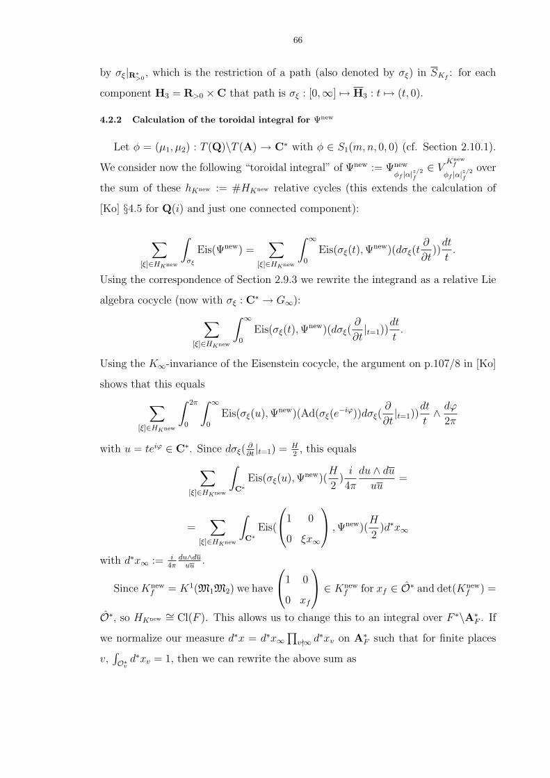
66

by σξ|R∗>0, which is the restriction of a path (also denoted by σξ) in SKf

: for each

component H3 = R>0 ×C that path is σξ : [0,∞] 7→ H3 : t 7→ (t, 0).

4.2.2 Calculation of the toroidal integral for Ψnew

Let φ = (µ1, µ2) : T (Q)\T (A) → C∗ with φ ∈ S1(m,n, 0, 0) (cf. Section 2.10.1).

We consider now the following “toroidal integral” of Ψnew := Ψnew

φf |α|z/2f

∈ VKnew

f

φf |α|z/2f

over

the sum of these hKnew := #HKnew relative cycles (this extends the calculation of

[Ko] §4.5 for Q(i) and just one connected component):

∑

[ξ]∈HKnew

∫

σξ

Eis(Ψnew) =∑

[ξ]∈HKnew

∫ ∞

0

Eis(σξ(t), Ψnew)(dσξ(t

∂

∂t))

dt

t.

Using the correspondence of Section 2.9.3 we rewrite the integrand as a relative Lie

algebra cocycle (now with σξ : C∗ → G∞):

∑

[ξ]∈HKnew

∫ ∞

0

Eis(σξ(t), Ψnew)(dσξ(

∂

∂t|t=1))

dt

t.

Using the K∞-invariance of the Eisenstein cocycle, the argument on p.107/8 in [Ko]

shows that this equals

∑

[ξ]∈HKnew

∫ 2π

0

∫ ∞

0

Eis(σξ(u), Ψnew)(Ad(σξ(e−iϕ))dσξ(

∂

∂t|t=1))

dt

t∧ dϕ

2π

with u = teiϕ ∈ C∗. Since dσξ(∂∂t|t=1) = H

2, this equals

∑

[ξ]∈HKnew

∫

C∗Eis(σξ(u), Ψnew)(

H

2)

i

4π

du ∧ du

uu=

=∑

[ξ]∈HKnew

∫

C∗Eis(

1 0

0 ξx∞

, Ψnew)(

H

2)d∗x∞

with d∗x∞ := i4π

du∧duuu

.

Since Knewf = K1(M1M2) we have

1 0

0 xf

∈ Knew

f for xf ∈ O∗ and det(Knewf ) =

O∗, so HKnew ∼= Cl(F ). This allows us to change this to an integral over F ∗\A∗F . If

we normalize our measure d∗x = d∗x∞∏

v-∞ d∗xv on A∗F such that for finite places

v,∫O∗v d∗xv = 1, then we can rewrite the above sum as

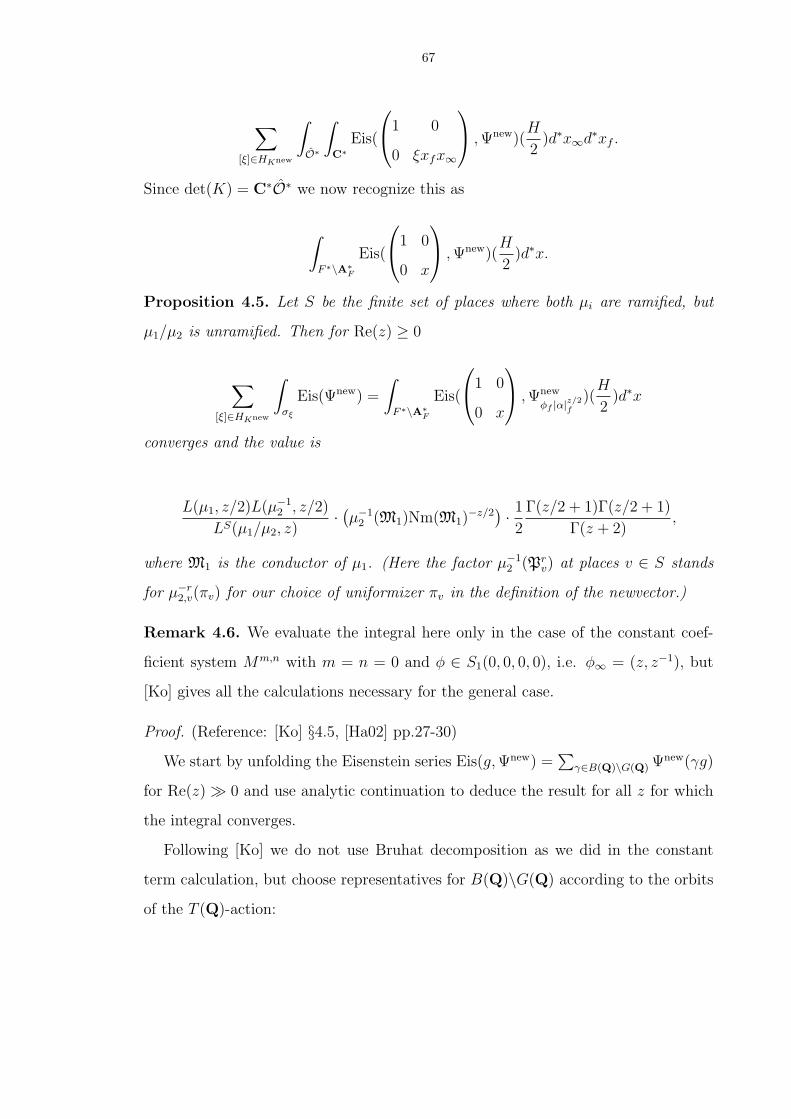
67

∑

[ξ]∈HKnew

∫

O∗

∫

C∗Eis(

1 0

0 ξxfx∞

, Ψnew)(

H

2)d∗x∞d∗xf .

Since det(K) = C∗O∗ we now recognize this as

∫

F ∗\A∗F

Eis(

1 0

0 x

, Ψnew)(

H

2)d∗x.

Proposition 4.5. Let S be the finite set of places where both µi are ramified, but

µ1/µ2 is unramified. Then for Re(z) ≥ 0

∑

[ξ]∈HKnew

∫

σξ

Eis(Ψnew) =

∫

F ∗\A∗F

Eis(

1 0

0 x

, Ψnew

φf |α|z/2f

)(H

2)d∗x

converges and the value is

L(µ1, z/2)L(µ−12 , z/2)

LS(µ1/µ2, z)· (µ−1

2 (M1)Nm(M1)−z/2

) · 1

2

Γ(z/2 + 1)Γ(z/2 + 1)

Γ(z + 2),

where M1 is the conductor of µ1. (Here the factor µ−12 (Pr

v) at places v ∈ S stands

for µ−r2,v(πv) for our choice of uniformizer πv in the definition of the newvector.)

Remark 4.6. We evaluate the integral here only in the case of the constant coef-

ficient system Mm,n with m = n = 0 and φ ∈ S1(0, 0, 0, 0), i.e. φ∞ = (z, z−1), but

[Ko] gives all the calculations necessary for the general case.

Proof. (Reference: [Ko] §4.5, [Ha02] pp.27-30)

We start by unfolding the Eisenstein series Eis(g, Ψnew) =∑

γ∈B(Q)\G(Q) Ψnew(γg)

for Re(z) À 0 and use analytic continuation to deduce the result for all z for which

the integral converges.

Following [Ko] we do not use Bruhat decomposition as we did in the constant

term calculation, but choose representatives for B(Q)\G(Q) according to the orbits

of the T (Q)-action:

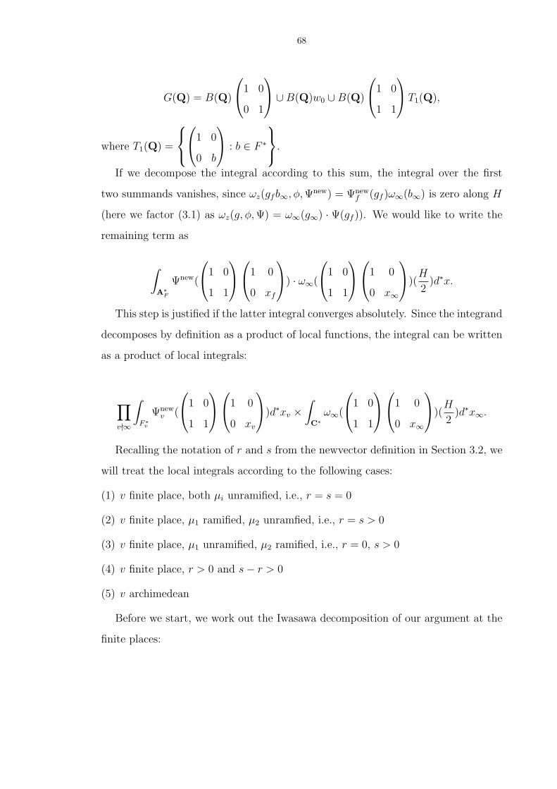
68

G(Q) = B(Q)

1 0

0 1

∪B(Q)w0 ∪B(Q)

1 0

1 1

T1(Q),

where T1(Q) =

1 0

0 b

: b ∈ F ∗

.

If we decompose the integral according to this sum, the integral over the first

two summands vanishes, since ωz(gfb∞, φ, Ψnew) = Ψnewf (gf )ω∞(b∞) is zero along H

(here we factor (3.1) as ωz(g, φ, Ψ) = ω∞(g∞) · Ψ(gf )). We would like to write the

remaining term as

∫

A∗F

Ψnew(

1 0

1 1

1 0

0 xf

) · ω∞(

1 0

1 1

1 0

0 x∞

)(

H

2)d∗x.

This step is justified if the latter integral converges absolutely. Since the integrand

decomposes by definition as a product of local functions, the integral can be written

as a product of local integrals:

∏

v-∞

∫

F ∗v

Ψnewv (

1 0

1 1

1 0

0 xv

)d∗xv ×

∫

C∗ω∞(

1 0

1 1

1 0

0 x∞

)(

H

2)d∗x∞.

Recalling the notation of r and s from the newvector definition in Section 3.2, we

will treat the local integrals according to the following cases:

(1) v finite place, both µi unramified, i.e., r = s = 0

(2) v finite place, µ1 ramified, µ2 unramfied, i.e., r = s > 0

(3) v finite place, µ1 unramified, µ2 ramified, i.e., r = 0, s > 0

(4) v finite place, r > 0 and s− r > 0

(5) v archimedean

Before we start, we work out the Iwasawa decomposition of our argument at the

finite places:

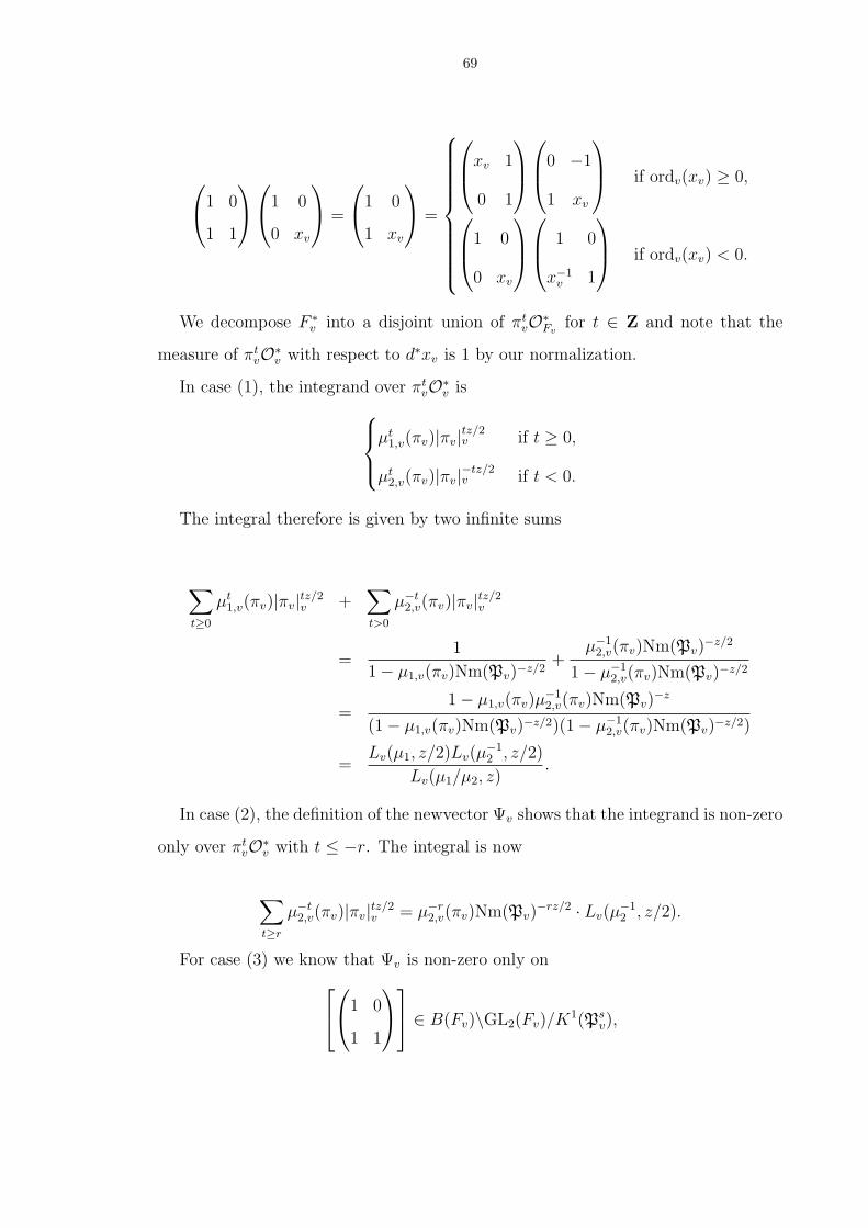
69

1 0

1 1

1 0

0 xv

=

1 0

1 xv

=

xv 1

0 1

0 −1

1 xv

if ordv(xv) ≥ 0,

1 0

0 xv

1 0

x−1v 1

if ordv(xv) < 0.

We decompose F ∗v into a disjoint union of πt

vO∗Fv

for t ∈ Z and note that the

measure of πtvO∗

v with respect to d∗xv is 1 by our normalization.

In case (1), the integrand over πtvO∗

v is

µt1,v(πv)|πv|tz/2

v if t ≥ 0,

µt2,v(πv)|πv|−tz/2

v if t < 0.

The integral therefore is given by two infinite sums

∑t≥0


v +∑t>0

µ−t2,v(πv)|πv|tz/2

v

=1

1− µ1,v(πv)Nm(Pv)−z/2+

µ−12,v(πv)Nm(Pv)

−z/2

1− µ−12,v(πv)Nm(Pv)−z/2

=1− µ1,v(πv)µ

−12,v(πv)Nm(Pv)

−z

(1− µ1,v(πv)Nm(Pv)−z/2)(1− µ−12,v(πv)Nm(Pv)−z/2)

=Lv(µ1, z/2)Lv(µ

−12 , z/2)

Lv(µ1/µ2, z).

In case (2), the definition of the newvector Ψv shows that the integrand is non-zero

only over πtvO∗

v with t ≤ −r. The integral is now

∑t≥r

µ−t2,v(πv)|πv|tz/2

v = µ−r2,v(πv)Nm(Pv)

−rz/2 · Lv(µ−12 , z/2).

For case (3) we know that Ψv is non-zero only on

1 0

1 1

∈ B(Fv)\GL2(Fv)/K

1(Psv),

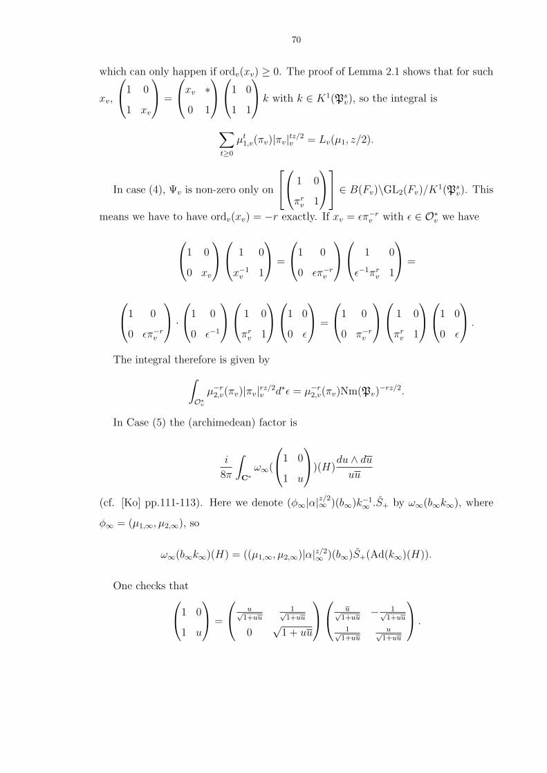
70

which can only happen if ordv(xv) ≥ 0. The proof of Lemma 2.1 shows that for such

xv,

1 0

1 xv

=

xv ∗

0 1

1 0

1 1

k with k ∈ K1(Ps

v), so the integral is

∑t≥0


v = Lv(µ1, z/2).

In case (4), Ψv is non-zero only on

1 0

πrv 1

∈ B(Fv)\GL2(Fv)/K

1(Psv). This

means we have to have ordv(xv) = −r exactly. If xv = επ−rv with ε ∈ O∗

v we have

1 0

0 xv

1 0

x−1v 1

=

1 0

0 επ−rv

1 0

ε−1πrv 1

=

1 0

0 επ−rv

·

1 0

0 ε−1

1 0

πrv 1

1 0

0 ε

=

1 0

0 π−rv

1 0

πrv 1

1 0

0 ε

.

The integral therefore is given by

∫

O∗vµ−r

2,v(πv)|πv|rz/2v d∗ε = µ−r

2,v(πv)Nm(Pv)−rz/2.

In Case (5) the (archimedean) factor is

i

8π

∫

C∗ω∞(

1 0

1 u

)(H)

du ∧ du

uu

(cf. [Ko] pp.111-113). Here we denote (φ∞|α|z/2∞ )(b∞)k−1

∞ .S+ by ω∞(b∞k∞), where

φ∞ = (µ1,∞, µ2,∞), so

ω∞(b∞k∞)(H) = ((µ1,∞, µ2,∞)|α|z/2∞ )(b∞)S+(Ad(k∞)(H)).

One checks that1 0

1 u

=

u√1+uu

1√1+uu

0√

1 + uu

u√1+uu

− 1√1+uu

1√1+uu

u√1+uu

.

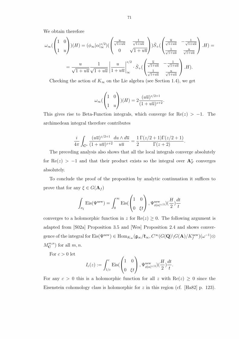
71

We obtain therefore

ω∞(

1 0

1 u

)(H) = (φ∞|α|z/2

∞ )(

u√1+uu

1√1+uu

0√

1 + uu

)S+(

u√1+uu

− 1√1+uu

1√1+uu

u√1+uu

.H) =

=u√

1 + uu

1√1 + uu

∣∣∣∣u

1 + uu

∣∣∣∣z/2

∞· S+(

u√1+uu

− 1√1+uu

1√1+uu

u√1+uu

.H).

Checking the action of K∞ on the Lie algebra (see Section 1.4), we get

ω∞(

1 0

1 u

)(H) = 2

(uu)z/2+1

(1 + uu)z+2.

This gives rise to Beta-Function integrals, which converge for Re(z) > −1. The

archimedean integral therefore contributes

i

4π

∫

C∗

(uu)z/2+1

(1 + uu)z+2

du ∧ du

uu=

1

2

Γ(z/2 + 1)Γ(z/2 + 1)

Γ(z + 2).

The preceding analysis also shows that all the local integrals converge absolutely

for Re(z) > −1 and that their product exists so the integral over A∗F converges

absolutely.

To conclude the proof of the proposition by analytic continuation it suffices to

prove that for any ξ ∈ G(Af )

∫

σξ

Eis(Ψnew) =

∫ ∞

0

Eis(

1 0

0 ξt

, Ψnew

φ|α|z/2)(H

2)dt

t

converges to a holomorphic function in z for Re(z) ≥ 0. The following argument is

adapted from [S02a] Proposition 3.5 and [Wes] Proposition 2.4 and shows conver-

gence of the integral for Eis(Ψnew) ∈ HomK∞(g∞/k∞, C∞(G(Q)\G(A)/Knewf )(ω−1)⊗

Mm,nC ) for all m,n.

For c > 0 let

Ic(z) :=

∫ c

1/c

Eis(

1 0

0 ξt

, Ψnew

φ|α|z/2)(H

2)dt

t.

For any c > 0 this is a holomorphic function for all z with Re(z) ≥ 0 since the

Eisenstein cohomology class is holomorphic for z in this region (cf. [Ha82] p. 123).

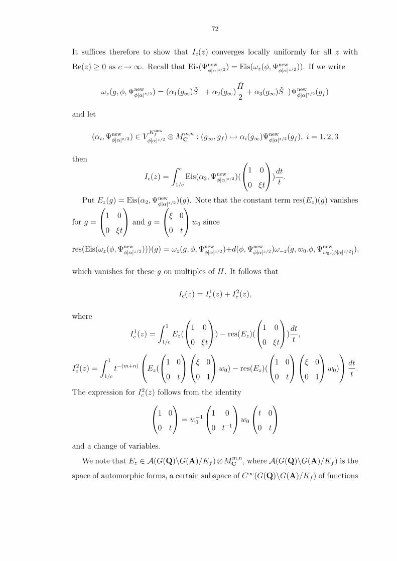
72

It suffices therefore to show that Ic(z) converges locally uniformly for all z with

Re(z) ≥ 0 as c →∞. Recall that Eis(Ψnewφ|α|z/2) = Eis(ωz(φ, Ψnew

φ|α|z/2)). If we write

ωz(g, φ, Ψnewφ|α|z/2) = (α1(g∞)S+ + α2(g∞)

H

2+ α3(g∞)S−)Ψnew

φ|α|z/2(gf )

and let

(αi, Ψnewφ|α|z/2) ∈ V

Knewf

φ|α|z/2 ⊗Mm,nC : (g∞, gf ) 7→ αi(g∞)Ψnew

φ|α|z/2(gf ), i = 1, 2, 3

then

Ic(z) =

∫ c

1/c

Eis(α2, Ψnewφ|α|z/2)(

1 0

0 ξt

)

dt

t.

Put Ez(g) = Eis(α2, Ψnewφ|α|z/2)(g). Note that the constant term res(Ez)(g) vanishes

for g =

1 0

0 ξt

and g =

ξ 0

0 t

w0 since

res(Eis(ωz(φ, Ψnewφ|α|z/2)))(g) = ωz(g, φ, Ψnew

φ|α|z/2)+d(φ, Ψnewφ|α|z/2)ω−z(g, w0.φ, Ψnew

w0.(φ|α|z/2)),

which vanishes for these g on multiples of H. It follows that

Ic(z) = I1c (z) + I2

c (z),

where

I1c (z) =

∫ 1

1/c

Ez(

1 0

0 ξt

)− res(Ez)(

1 0

0 ξt

)

dt

t,

I2c (z) =

∫ 1

1/c

t−(m+n)

Ez(

1 0

0 t

ξ 0

0 1

w0)− res(Ez)(

1 0

0 t

ξ 0

0 1

w0)

dt

t.

The expression for I2c (z) follows from the identity

1 0

0 t

= w−1

0

1 0

0 t−1

w0

t 0

0 t

and a change of variables.

We note that Ez ∈ A(G(Q)\G(A)/Kf )⊗Mm,nC , where A(G(Q)\G(A)/Kf ) is the

space of automorphic forms, a certain subspace of C∞(G(Q)\G(A)/Kf ) of functions

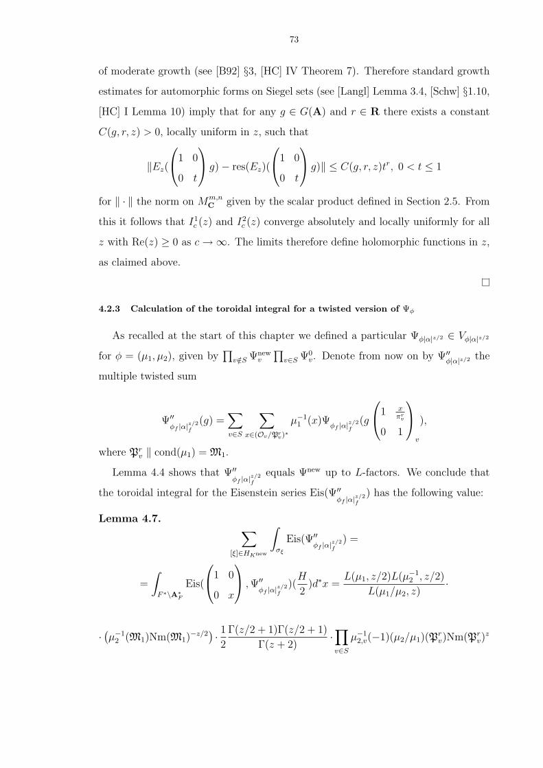
73

of moderate growth (see [B92] §3, [HC] IV Theorem 7). Therefore standard growth

estimates for automorphic forms on Siegel sets (see [Langl] Lemma 3.4, [Schw] §1.10,

[HC] I Lemma 10) imply that for any g ∈ G(A) and r ∈ R there exists a constant

C(g, r, z) > 0, locally uniform in z, such that

‖Ez(

1 0

0 t

g)− res(Ez)(

1 0

0 t

g)‖ ≤ C(g, r, z)tr, 0 < t ≤ 1

for ‖ · ‖ the norm on Mm,nC given by the scalar product defined in Section 2.5. From

this it follows that I1c (z) and I2

c (z) converge absolutely and locally uniformly for all

z with Re(z) ≥ 0 as c →∞. The limits therefore define holomorphic functions in z,

as claimed above.

4.2.3 Calculation of the toroidal integral for a twisted version of Ψφ

As recalled at the start of this chapter we defined a particular Ψφ|α|z/2 ∈ Vφ|α|z/2

for φ = (µ1, µ2), given by∏

v/∈S Ψnewv

∏v∈S Ψ0

v. Denote from now on by Ψ′′φ|α|z/2 the

multiple twisted sum

Ψ′′φf |α|z/2

f

(g) =∑v∈S

∑

x∈(Ov/Prv)∗

µ−11 (x)Ψ

φf |α|z/2f

(g

1 x

πrv

0 1

v

),

where Prv ‖ cond(µ1) = M1.

Lemma 4.4 shows that Ψ′′φf |α|z/2

f

equals Ψnew up to L-factors. We conclude that

the toroidal integral for the Eisenstein series Eis(Ψ′′φf |α|z/2

f

) has the following value:

Lemma 4.7.∑

[ξ]∈HKnew

∫

σξ

Eis(Ψ′′φf |α|z/2

f

) =

=

∫

F ∗\A∗F

Eis(

1 0

0 x

, Ψ′′

φf |α|z/2f

)(H

2)d∗x =

L(µ1, z/2)L(µ−12 , z/2)

L(µ1/µ2, z)·

· (µ−12 (M1)Nm(M1)

−z/2) · 1

2

Γ(z/2 + 1)Γ(z/2 + 1)

Γ(z + 2)·∏v∈S

µ−12,v(−1)(µ2/µ1)(P

rv)Nm(Pr

v)z

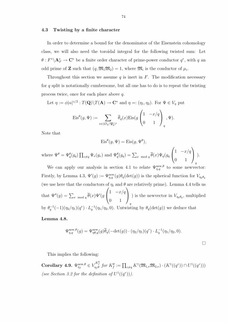
74

4.3 Twisting by a finite character

In order to determine a bound for the denominator of the Eisenstein cohomology

class, we will also need the toroidal integral for the following twisted sum: Let

θ : F ∗\A∗F → C∗ be a finite order character of prime-power conductor qr, with q an

odd prime of Z such that (q, M1M2) = 1, where Mi is the conductor of µi.

Throughout this section we assume q is inert in F . The modification necessary

for q split is notationally cumbersome, but all one has to do is to repeat the twisting

process twice, once for each place above q.

Let η := φ|α|z/2 : T (Q)\T (A) → C∗ and η =: (η1, η2). For Ψ ∈ Vη put

Eisθ(g, Ψ) :=∑

x∈(Oq/Prq)∗

θq(x)Eis(g

1 −x/q

0 1

q

, Ψ).

Note that

Eisθ(g, Ψ) = Eis(g, Ψθ),

where Ψθ = Ψθq(gq)

∏v 6=q Ψv(gv) and Ψθ

q(gq) =∑

x mod q θ(x)Ψq(gq

1 −x/q

0 1

q

).

We can apply our analysis in section 4.1 to relate Ψnew,θη,q to some newvector:

Firstly, by Lemma 4.3, Ψ′(g) := Ψnewη,q (g)θq(det(g)) is the spherical function for Vηqθq

(we use here that the conductors of ηi and θ are relatively prime). Lemma 4.4 tells us

that Ψ′′(g) =∑

x mod q θ(x)Ψ′(g

1 −x/q

0 1

q

) is the newvector in Vηqθq , multiplied

by θ−1q (−1)(η2/η1)(q

r) · L−1q (η1/η2, 0). Untwisting by θq(det(g)) we deduce that

Lemma 4.8.

Ψnew,θη,q (g) = Ψnew

ηθ,q(g)θq(−det(g)) · (η2/η1)(qr) · L−1

q (η1/η2, 0).

This implies the following:

Corollary 4.9. Ψnew,θηf

∈ VKθ

f

ηf θ for Kθf :=

∏v 6=q K1(M1,vM2,v) · (K1((qr)) ∩ U1((qr)))

(see Section 3.2 for the definition of U1((qr))).

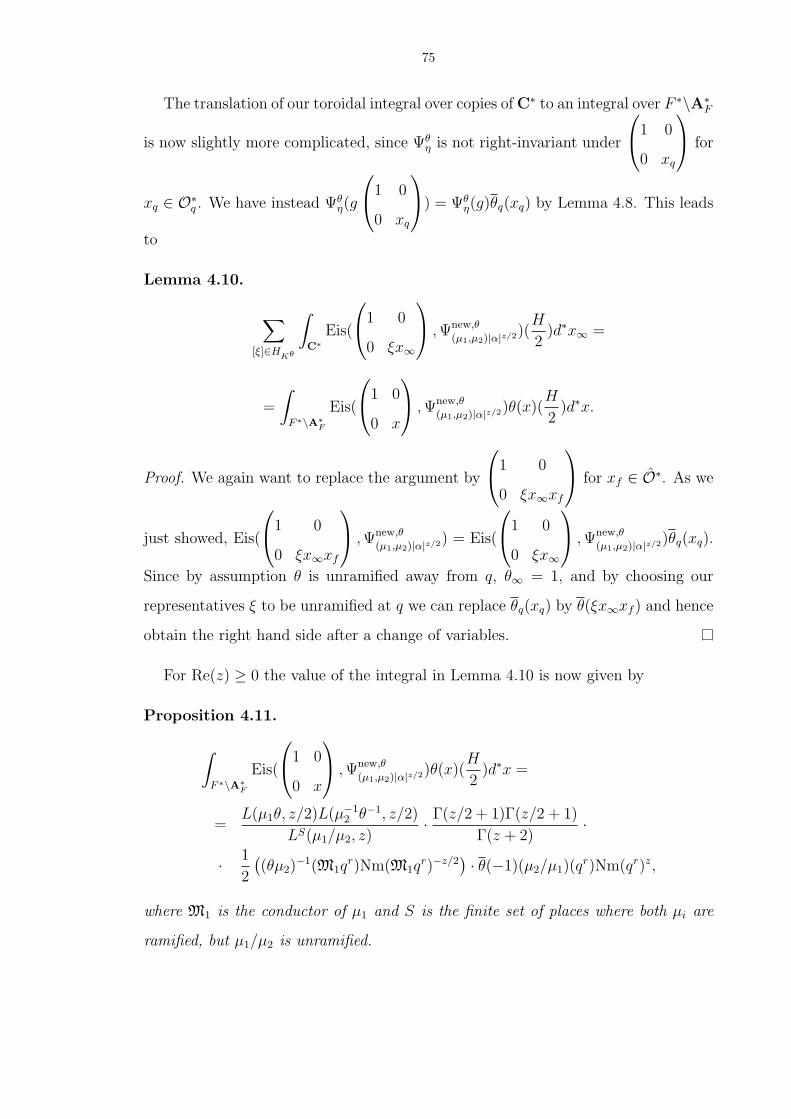
75

The translation of our toroidal integral over copies of C∗ to an integral over F ∗\A∗F

is now slightly more complicated, since Ψθη is not right-invariant under

1 0

0 xq

for

xq ∈ O∗q . We have instead Ψθ

η(g

1 0

0 xq

) = Ψθ

η(g)θq(xq) by Lemma 4.8. This leads

to

Lemma 4.10.

∑

[ξ]∈HKθ

∫

C∗Eis(

1 0

0 ξx∞

, Ψnew,θ

(µ1,µ2)|α|z/2)(H

2)d∗x∞ =

=

∫

F ∗\A∗F

Eis(

1 0

0 x

, Ψnew,θ

(µ1,µ2)|α|z/2)θ(x)(H

2)d∗x.

Proof. We again want to replace the argument by

1 0

0 ξx∞xf

for xf ∈ O∗. As we

just showed, Eis(

1 0

0 ξx∞xf

, Ψnew,θ

(µ1,µ2)|α|z/2) = Eis(

1 0

0 ξx∞

, Ψnew,θ

(µ1,µ2)|α|z/2)θq(xq).

Since by assumption θ is unramified away from q, θ∞ = 1, and by choosing our

representatives ξ to be unramified at q we can replace θq(xq) by θ(ξx∞xf ) and hence

obtain the right hand side after a change of variables.

For Re(z) ≥ 0 the value of the integral in Lemma 4.10 is now given by

Proposition 4.11.

∫

F ∗\A∗F

Eis(

1 0

0 x

, Ψnew,θ

(µ1,µ2)|α|z/2)θ(x)(H

2)d∗x =

=L(µ1θ, z/2)L(µ−1

2 θ−1, z/2)

LS(µ1/µ2, z)· Γ(z/2 + 1)Γ(z/2 + 1)

Γ(z + 2)·

· 1

2

((θµ2)

−1(M1qr)Nm(M1q

r)−z/2) · θ(−1)(µ2/µ1)(q

r)Nm(qr)z,

where M1 is the conductor of µ1 and S is the finite set of places where both µi are

ramified, but µ1/µ2 is unramified.

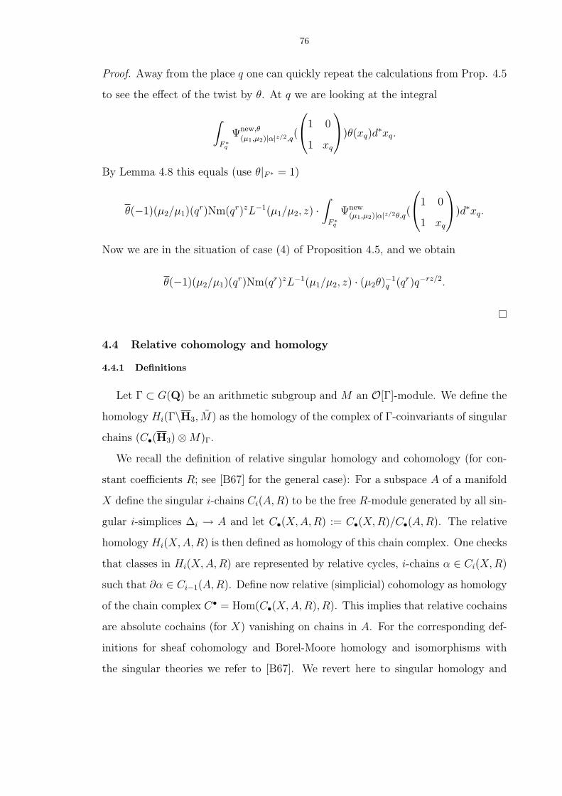
76

Proof. Away from the place q one can quickly repeat the calculations from Prop. 4.5

to see the effect of the twist by θ. At q we are looking at the integral

∫

F ∗q

Ψnew,θ

(µ1,µ2)|α|z/2,q(

1 0

1 xq

)θ(xq)d

∗xq.

By Lemma 4.8 this equals (use θ|F ∗ = 1)

θ(−1)(µ2/µ1)(qr)Nm(qr)zL−1(µ1/µ2, z) ·

∫

F ∗q

Ψnew(µ1,µ2)|α|z/2θ,q(

1 0

1 xq

)d∗xq.

Now we are in the situation of case (4) of Proposition 4.5, and we obtain

θ(−1)(µ2/µ1)(qr)Nm(qr)zL−1(µ1/µ2, z) · (µ2θ)

−1q (qr)q−rz/2.

4.4 Relative cohomology and homology

4.4.1 Definitions

Let Γ ⊂ G(Q) be an arithmetic subgroup and M an O[Γ]-module. We define the

homology Hi(Γ\H3, M) as the homology of the complex of Γ-coinvariants of singular

chains (C•(H3)⊗M)Γ.

We recall the definition of relative singular homology and cohomology (for con-

stant coefficients R; see [B67] for the general case): For a subspace A of a manifold

X define the singular i-chains Ci(A, R) to be the free R-module generated by all sin-

gular i-simplices ∆i → A and let C•(X,A, R) := C•(X, R)/C•(A,R). The relative

homology Hi(X, A, R) is then defined as homology of this chain complex. One checks

that classes in Hi(X,A, R) are represented by relative cycles, i-chains α ∈ Ci(X, R)

such that ∂α ∈ Ci−1(A,R). Define now relative (simplicial) cohomology as homology

of the chain complex C• = Hom(C•(X, A, R), R). This implies that relative cochains

are absolute cochains (for X) vanishing on chains in A. For the corresponding def-

initions for sheaf cohomology and Borel-Moore homology and isomorphisms with

the singular theories we refer to [B67]. We revert here to singular homology and

77

cohomology because we want to make use of the explicit evaluation pairings between

them.

Proposition 4.12 ([F], Satz 3, [G67] §23). 1. For the ring R = O[16] and a

subspace A ⊂ Γ\H3 the evaluation pairing

Hi(Γ\H3, A, M∨ ⊗R)/torsion×H i(Γ\H3, A, M ⊗R)/torsion → R

is perfect and functorial in the ring R.

2. For R = C, the pairing between a de Rham (or relative Lie algebra) cocycle ω

and a differentiable singular cycle σ is given by the integral

∫

σ

ω.

4.4.2 Interpretation of the toroidal integral as evaluation pairing

We have [Eisθ(Ψ′′φ)] ∈ H1(SKθ

f,C). Here φ = (µ1, µ2) : T (Q)\T (A) → C∗. Let

SKθf

∼=⊕

[det(ξ)]∈HKθ

Γθξ\H3.

The paths σξ we described in 4.2.1 are not 1-cycles in SKθf. They are only relative

cycles (cf. [Ko] §5.2) giving rise to classes in H1(Γθξ\H3, ∂(Γθ

ξ\H3),Z). Since the

endpoints lie in the ∞- and 0-cusps (use

1 0

0 1s

K∞ = w0

1 0

0 s

K∞) they are,

in fact, relative cycles for H1(Γθξ\H3, Γ

θξ,B\e(B) ∪ Γθ

ξ,Bw\e(Bw),Z).

If we can show that Eisθ(Ψ′′φ) is a relative cocycle with respect to the ∞- and

0-cusps of each connected component, we can apply the evaluation pairing

H1(Γθξ\H3, e

′(B) ∪ e′(Bw), R)×H1(Γθξ\H3, e

′(B) ∪ e′(Bw),Z) → R,

given by ([ω], [σξ]) 7→∫

σξω (here we follow [BS] in writing e′(P ) for Γθ

ξ,P\e(P )). By

the functoriality in the O-algebra R, a multiple aω is integral only if a([ω], [σξ]) is.

Our toroidal integral now corresponds to the sum of these evaluation pairings for

each connected component. This allows us in the next section to deduce a lower

78

bound on the denominator of the Eisenstein cohomology class in terms of a special

L-value. We will show that the result of the toroidal integral is the inverse of the

special L-value up to p-adic units.

We prove now:

Lemma 4.13. Let Fθ be the finite extension of Fχ (see Definition 3.22) containing

the values of the finite order character θ. Then we have

[Eisθ(Ψ′′φ)] ∈

⊕

[det(ξ)]∈HKθ

H1(Γθξ\H3, e

′(B) ∪ e′(Bw), Fθ).

Proof. It is clear that [Eisθ(Ψ′′φ)] ∈ H1(SKθ

f, Fθ). From the form of the constant term

for res(Eis(ω0(φ, Ψφ))) (see Proposition 3.5) we deduce, by interchanging the finite

sums of the twists with the integral, that

res(Eisθ(Ψ′′φ)) = res(Eisθ(ω0(φ, Ψ′′

φ))) = ω0(φ, (Ψ′′φ)

θ) + d(φ)ω0(w0.φ, (Ψ′′w0.φ)

θ).

Here

(Ψ′′∗)

θ(g) =∑

x

θ(x)Ψ′′∗(g

1 −x/q

0 1

q

).

To check that the Eisenstein cocycle vanishes on 1-cycles of e′(B)∪e′(Bw) we now

translate to group cohomology and homology. We showed in Lemma 3.10 that the

restriction of [ω0(∗ · θ, (Ψ′′∗)

θ)] to H1(Γθξ,Bη\e(Bη), Fθ) ∼= H1(Γθ

ξ,Bη , Fθ) is represented

by the cocycle

η−1

a x

0 d

η 7→ (Ψ′′

∗)θ(ηfξ) ·

x

x

,

the two cases depending on the infinity type of ∗.We need to show therefore that (Ψ′′

∗)θ vanishes on ηfξ for η the identity matrix and

w0. We note that ξ ∈ G(Af ) can be chosen to be a diagonal matrix. Then vanishing

for η equal to the identity matrix follows immediately from∑

x∈(Oq/Prq)∗ θ(x) = 0 for

the finite order character θ. For η = w0 the vanishing follows from our definition of

the newvectors Ψnew∗ , of which Ψ′′

∗ is a multiple, and from our choice of q distinct

from the conductors of the characters µ1 and µ2.

79

4.4.3 Comparison with other methods

We briefly comment on other approaches to interpreting the toroidal integral. The

following method is used by Harder in [Ha02] for SL2(Z), in [Ko] §5.4 for Q(i), and

in [Ka] §5 for Γ1(p) ⊂ SL2(Z): Complete the relative cycles σξ (or rather their images

under powers of Tv for v the place corresponding to p) by a chain in H1(∂SKf,Z)

that is only supported on the infinity components of cusps “above 0”. Then the

evaluation pairing between an Eisenstein cohomology class supported only at cusps

“above ∞” and the completed cycle is given by the toroidal integral. However, when

these cusps coincide the calculation of the additional “boundary integral” and the

bounding of its denominator is non-trivial.

Kaiser [Ka] uses a twisting argument similar to the one in the next section (but for

the cycles, not the cohomology class) to deduce lower bounds for the denominator.

Our approach seems to explain why he can choose cycles such that the boundary

integrals vanish and provides a shorter alternative argument.

Skinner [S02a] gives a different interpretation of the toroidal integral. In [S02a]

§4 he introduces a theory of “partial Borel-Serre compactifications”. He reinterprets

the twisted Eisenstein cocycle Eisθ(Ψ′′) as a cocycle in the cohomology of the space

SKθf

⋃ξ(e

′(B) ∪ e′(Bw0)), which contains the closure of the σξ in SKθf. Since the

restriction of the twisted Eisenstein cohomology class to these cusps is trivial Eisθ(Ψ′′)

corresponds to a class cθ in H1c (SKθ

f

⋃ξ(e

′(B)∪e′(Bw0)),C). He shows that cθ is again

rational (in some finite extension of Fχ), and that if a ·Eisθ(Ψ′′) is integral, then a ·cθ

is, too. He considers for each connected component of SKfthe map of manifolds

σξ|R>0 : R>0 → jξ(Γξ\H3) ⊂ SKf.

This is a proper embedding giving rise to a map

σ∗ξ : H1c (SKθ

f

⋃

ξ

(e′(B) ∪ e′(Bw0)), R) → H1c (R>0, R) = H1

c (R>0,Z)⊗R ∼= R,

which is functorial in R and maps cθ to∫

σξEisθ(Ψ′′).

80

4.5 Bounding the denominator

Recall the definition of the denominator of a cohomology class from Definition

4.1. We are interested in bounding δ(Eis(Ψφ)) for the Ψφ defined in Section 3.2.

From now on, we consider an odd prime p of Z split in F and let p ⊂ O be one

of the primes dividing it. Let φ = (µ1, µ2) : T (Q)\T (A) → C∗ for µ1 and µ2 Hecke

characters with infinity type z and z−1, respectively, such that the conductors Mi of

µi are coprime to (p). Denote by Oφ the ring of integers in the finite extension of Fp

containing the values of µ1,f , µ2,f and Lalg(0, µ1/µ2). Here we use Theorem 2.1 on

the algebraicity and integrality of the special L-value.

For a finite order character θ of prime power conductor qr, with q a prime in

Z distinct from p and coprime to the conductors of the µi, let Oθ be the ring of

integers in the finite extension of Oφ containing the values of θ, Lalg(0, µ1θ), and

Lalg(0, (µ2θ)−1) (again we use Theorem 2.1).

Observe that

δ([Eis(Ψφ)]) ⊆ δ([Eis(Ψ′′φ)]) ⊆ Oφ,

and

δ([Eis(Ψ′′φ)])Oθ ⊆ δ([Eisθ(Ψ′′

φ)]).

In Section 4.4 we showed that the toroidal integral∑

[ξ]∈HKθ

∫σξ

Eisθ(Ψ′′φ) gives the

value of sums of evaluation pairings between relative cohomology and homology.

Their functoriality in the coefficient system implies that the denominator δ([Eisθ(Ψ′′φ)])

is bounded below by the denominator of the integral. Proposition 4.11 (for z=0) and

Lemma 4.4 imply that the integral equals L(0,µ1θ)L(0,(µ2θ)−1)L(0,µ1/µ2)

, up to units in Oθ (using

Lemma 3.21 one checks that

(θµ2)−1(M1q

r)θ(−1)(µ2/µ1)(qr)

1

2

∏v∈S

µ−12,v(−1)(µ2/µ1)(P

rv) ∈ O∗

θ .)

This means that δ([Eisθ(Ψ′′φ)]) is contained in the (possibly fractional) ideal(

L(0, µ1/µ2)

L(0, µ1θ)L(0, (µ2θ)−1)

)Oθ.

81

We would like to find finite order anticyclotomic characters θ such that the (al-

gebraic) L-factors in the denominator are p-adic units. We have at our disposal two

results on the non-vanishing modulo p of the L-values Lalg(0, θµ±1i ) as θ varies in an

anticyclotomic Zq-extension:

Theorem 4.14 (Finis [Fi2] Thm. 1.1). Let q - 2#Cl(F ) be a prime split in F ,

distinct from p. Consider Hecke characters λ of infinity type λ∞(z) = zkz1−k for a

fixed positive integer k with λ∗ = λ (where λ∗(x) = λ(x)−1|x|AF), conductor dividing

ddF q∞ for some fixed d, global root number W (λ) = 1, and such that no inert primes

congruent to -1 mod p divide the conductor of λ with multiplicity one. Then for all

but finitely many such Hecke characters

L(0, λ)Wp(λ)Ω1−2k(k − 1)!(2π√dF

)k−1 is a p− adic unit.

The p-adic root number Wp(λ) is defined as p−ordv0 (fλ) · τv0(λv0) for v0 the place

corresponding to p. For the definition of the Gauss sum τv0 see Section 2.6.

Hida has announced a similar result (for general CM fields). The pre-print [Hi04b]

includes the theorem:

Theorem 4.15 ([Hi04b] Theorem 4.3). Fix a character λ of split conductor

(i.e., such that the conductor is a product of primes split in F/Q) with infinity type

λ∞(z) = zk(

zz

)lfor k > 0 and l ≥ 0. Then

Lalg(λθ, 0) is a p− adic unit

for all but finitely many finite-order anticyclotomic characters θ of q-power conductor

for a split prime q distinct from p and coprime to the conductor of λ.

From these two results we deduce the following:

Proposition 4.16. Let µ1, µ2 as above. Assume in addition that either

(a) the characters satisfy µci = µi (for this infinity type this coincides with µ∗i = µi)

and that no inert primes congruent to −1 mod p divide either of the conductors

of µi with multiplicity one

82

(b) or the characters µi have split conductor.

Then there exists a prime q and a finite order anticyclotomic character θ of q-power

conductor such that Lalg(0, µ1θ) and Lalg(0, (µ2θ)−1) lie in O∗

θ .

Proof. All that remains to show is that for (a) Wp(λ) is a p-adic unit (we take k = 1

in Finis’ Theorem). This follows from the definition of the Gauss sum and (the proof

of) Lemma 3.21.

With this we have also proven:

Theorem 4.17. Under the same assumptions as the previous proposition we have

δ([Eis(Ψφ)]) ⊆ Lalg(0, µ1/µ2)Oφ.

Theorem 1.2 in the introduction follows from Theorem 4.17:

Corollary 4.18 (Theorem 1.2). Let χ be a Hecke character of infinity type z2 such

that χc = χ. Assume also that no inert primes congruent to −1 mod p or factors

of p divide the conductor of χ. Then there exist characters µi such that χ = µ1/µ2

and δ([Eis(Ψ(µ1,µ2))]) ⊂ (Lalg(0, χ)).

Proof. It suffices to show that χ can be factored as µ1/µ2 with characters satisfying

the conditions of the previous theorem. Put µ1 = µGχ and µ2 = µG, where µG is

the character from Lemma 3.18. Since µG is ramified only at the ramified places

in F and satisfies µcG = µG this choice φ = (µ1, µ2) satisfies the condition (a) of

Proposition 4.16.

CHAPTER V

The torsion problem

Recall from Lemma 3.24 that [res(Eis(Ψ(µ1,µ2)))] ∈ H1(∂SKsf,Oχ) if we assume

χ = µ1/µ2 to be anticyclotomic (see Definition 3.22 for Oχ and Fχ). In Chapter VI

we will show that if we can find c ∈ H1(SKsf,Oχ) with the same restriction to the

boundary as our Eisenstein cohomology class [Eis(Ψ(µ1,µ2))] ∈ H1(SKsf, Fχ) then this

implies a congruence between a certain integral multiple of the Eisenstein cohomology

class and a cohomology class in H1! (SKf

,Oχ).

The aim of this chapter is to isolate cases where we can find such a class c, which

means ruling out congruences of the Hecke eigenvalues of our Eisenstein class with

those of torsion classes in H2c . The existence of such torsion classes was shown,

for example, in R. Taylor’s thesis [T], and in calculations by Feldhusen ([F] p.26).

We manage to avoid this “torsion problem” after restricting to constant coefficient

systems and unramified χ, and excluding the two fields Q(√−1) and Q(

√−3).

Our strategy is to find an involution on the boundary cohomology such that (for

each connected component of SKsf)

H1(Γ\H3,Oχ)res³ H1(∂(Γ\H3),Oχ)−,

where the superscript ‘-’ indicates the -1-eigenspace of this involution. We prove

the existence of such an involution for all maximal arithmetic subgroups of SL2(F ),

extending a result of Serre for SL2(O). After checking that [res(Eis(Ψ(µ1,µ2)))] lies in

this −1-eigenspace, we deduce the existence of the integral lift c.

83

84

5.1 Involutions and the image of the restriction map

In this section we work with a general arithmetic subgroup Γ. Assuming that we

have an orientation-reversing involution on Γ\H3 such that

H1(Γ\H3,Oχ)res→ H1(∂(Γ\H3),Oχ)−

we show that the map is, in fact, surjective. The existence of such an involution will

be shown for maximal arithmetic subgroups in the following sections.

We first recall:

Theorem 5.1 (Poincare and Lefschetz duality). Suppose Γ ⊂ G(Q) is an

arithmetic subgroup. Let R be a Dedekind domain in which both the lowest common

multiple of the orders of stabilizers |Γx| as well as the greatest common divisor of the

indices of torsion-free subgroups of finite index in Γ are invertible. Then there are

perfect pairings

Hrc (Γ\H3, R)×H3−r(Γ\H3, R) → R for 0 ≤ r ≤ 3

and

Hr(∂(Γ\H3), R)×H2−r(∂(Γ\H3), R) → R for 0 ≤ r ≤ 2.

Furthermore, the maps in the exact sequence

H1(Γ\H3, R)res−→ H1(∂(Γ\H3), R)

∂−→ H2c (Γ\H3, R)

are adjoint, i.e.,

〈res(x), y〉 = 〈x, ∂(y)〉.

Proof. Serre states this in the proof of Lemma 11 in [Se70] for field coefficients, [AS]

Lemma 1.4.3 proves the perfectness for fields R and [U95] Theorem 1.6 for Dedekind

domains as above. Other references for this Lefschetz or “relative” Poincare duality

for oriented manifolds with boundary are [Ma99] Chapter 21, §4 and [G67] (28.18).

We use here that H3 is an oriented manifold with boundary and that Γ acts on it

properly discontinuously and without reversing orientation.

85

For the following, we just want to recall the definition of the pairings: Write

M = Γ\H3. As explained in [Ma99] there is an unique element (called the R-

fundamental class) zΓ ∈ H3(M, ∂M,R) such that ∂zΓ is the fundamental class of

∂M ∈ H2(∂M,R) induced by the R-orientation of M . The pairings are then given

by the cup product and evaluation on the respective fundamental classes.

In particular, one deduces the following lemma:

Lemma 5.2 (Poincare duality and orientation-reversing involutions). Sup-

pose Γ and R are as in the theorem and that 2 is invertible in R. Let ι be an

orientation-reversing involution on Γ\H3. Denoting by a superscript + (resp. −)

the +1-(resp. −1-) eigenspaces for the induced involutions on cohomology groups,

we have perfect pairings

Hrc (Γ\H3, R)± ×H3−r(Γ\H3, R)∓ → R for 0 ≤ r ≤ 3

and

Hr(∂(Γ\H3), R)± ×H2−r(∂(Γ\H3), R)∓ → R for 0 ≤ r ≤ 2.

Proof. That ι reverses the orientation on Γ\H3 means exactly that ι(zΓ) = −zΓ for zΓ

as in the proof of the theorem. This implies that +1- and −1-eigenspaces are “self-

orthogonal” under the duality pairing, or maximal isotropic subspaces. Since the

perfect pairing for the boundary uses the fundamental class ∂zΓ the same argument

applies to the boundary after checking that the connecting homomorphism ∂ is ι-

equivariant.

Lemma 5.3. Suppose in addition to the conditions of the previous theorem and

lemma that R is a complete discrete valuation ring with finite residue field of char-

acteristic p > 2. Suppose that we have an involution ι as in the lemma such that

H1(Γ\H3, R)res→ H1(∂(Γ\H3), R)ε,

where ε = +1 or −1. Then, in fact, the restriction map is surjective.

86

Proof. Let m denote the maximal ideal of R. Since the cohomology modules are

finitely generated (so the Mittag-Leffler condition is satisfied for lim←−H1(·, R/mr)), it

suffices to prove the surjectivity for each r ∈ N of

H1(Γ\H3, R/mr) ³ H1(∂(Γ\H3), R/mr)ε.

For these coefficient systems we are dealing with finite groups and can count the

number of elements in the image and the eigenspace of the involution; they turn

out to be the same. We observe that H1(∂(Γ\H3), R/mr) = H1(∂(Γ\H3), R/mr)+⊕H1(∂(Γ\H3), R/mr)− and that, by the last lemma,

#H1(∂(Γ\H3), R/mr)+ = #H1(∂(Γ\H3), R/mr)−.

Similarly we deduce from the adjointness of res and ∂ and the perfectness of the

pairings that im(res)⊥ = im(res) and so

#im(res) =1

2#H1(∂(Γ\H3), R/mr).

5.2 The involution for SL2(O)

We first make the following observation that will simplify the treatment of the

cohomology of the boundary components:

Lemma 5.4. For imaginary quadratic fields F other than Q(√−1) or Q(

√−3),

Γ ⊂ SL2(F ) an arithmetic subgroup, P a parabolic subgroup of ResF/Q(SL2/F ) with

unipotent radical UP , and R a ring in which 2 is invertible we have

H1(ΓP , R) ∼= H1(ΓUP, R),

where ΓP = Γ ∩ P (Q) and ΓUP= Γ ∩ UP (Q).

Proof. Serre shows in [Se70] Lemme 7 that ΓUP/ ΓP and that the quotient WP =

ΓP /ΓUPcan be identified with a subgroup of the roots of unity of F, i.e., of ±1

since F 6= Q(√−1),Q(

√−3). We recall his argument here: Suppose P = Bη for

87

η ∈ G(Q) (where Bη(Q) = η−1B(Q)η). The parabolic Bη is the stabilizer of a cusp

Dη ∈ P1(F ), the latter determined by the isomorphism B(Q)\G(Q) ∼= P1(F ) given

by [η] = [

a b

c d

] 7→ Dη := [c : d]. If g ∈ Bη(Q) denote by ω(g) the element in F ∗

such that g.x = ω(g)x for all x ∈ Dη. One gets a short exact sequence

1 → Uη(Q) → Bη(Q)ω→ F ∗ → 1.

The eigenvalues of any element of an arithmetic subgroup are integral. In particular,

if g ∈ ΓBη then ω(g) ∈ O∗, and we have the short exact sequence

1 → ΓUη → ΓBηω→ O∗ → 1

which proves the claim made at the start.

By the Inflation-Restriction sequence we deduce now that

H1(ΓP , R)∼−→ H1(ΓUP

, R)WP

since #WB = 2 ∈ R∗. Now WB ⊂ ±1 acts trivially on ΓU , and therefore

H1(ΓP , R) ' H1(ΓUP, R).

For a general arithmetic subgroup Γ ⊂ G(Q), the set Bη : [η] ∈ B(Q)\G(Q)/Γis a set of representatives for the Γ-conjugacy classes of Borel subgroups. The group

Uη is the unipotent radical of Bη. For D ∈ P1(F ) let ΓD = Γ ∩ UD, where UD is

the unipotent subgroup of SL2(F ) fixing D. Note that if Dη ∈ P1(F ) corresponds

to [η] ∈ B(Q)\G(Q) under the isomorphism of B(Q)\G(Q) ∼= P1(F ) given by right

action on [0 : 1] ∈ P1(F ) (see also Lemma 5.4) we have that UDη = Uη(Q) and

ΓDη = Γ ∩ Uη(Q) = ΓUη .

Let U(Γ) be the direct sum ⊕[D]∈P1(F )/ΓΓD. Up to canonical isomorphism this is

independent of the choice of representatives [D] ∈ P1(F )/Γ. The inclusion ΓD → Γ

defines a homomorphism α : U(Γ) → Γab.

Serre studies in [Se70] the kernel of U(Γ) → Γab. For Γ = SL2(O) he shows

(by choosing an appropriate set of representatives of P1(F )/SL2(O ∼= Cl(F )) that

88

there is a well-defined action of complex conjugation on U(SL2(O)) induced by the

complex conjugation action on the matrix entries of G∞ = GL2(C). Denoting by

U+ the set of elements of U(SL2(O)) invariant under the involution and by U ′ the

set of elements u + u for u ∈ U(SL2(O)), his result is as follows:

Theorem 5.5 (Serre [Se70] Theoreme 9). For imaginary quadratic fields F

other than Q(√−1) or Q(

√−3) the kernel of the homomorphism α : U(SL2(O)) →SL2(O)ab satisfies the inclusions

6U ′ ⊆ ker(α) ⊆ U+.

For our purposes we reinterpret this as follows:

Corollary 5.6. For imaginary quadratic fields F other than Q(√−1) or Q(

√−3),

Γ = SL2(O), and R a ring in which 2 and 3 is invertible, the image of the restriction

map

H1(Γ\H3, R) → H1(∂(Γ\H3), R)

is contained in the −1-eigenspace of the involution induced by

ι : H3 = C×R>0 → H3 : (z, t) 7→ (z, t).

Proof. We first note that since SL2(O) (in fact, even GL2(F )) has only 2- and 3-

torsion (see Proof of Lemma 1.1 in [F]) we have an isomorphism H1(Γ\H3, R) ∼=H1(Γ, R) by Proposition 2.5. From Section 2.8 we know that ∂(Γ\H3) is homotopy

equivalent to∐

[η]∈P1(F )/Γ

ΓBη\H3,

where ΓBη = Γ ∩Bη. That we have, in fact,

H1(∂(Γ\H3), R) ∼=∐

[η]∈P1(F )/Γ

H1(ΓUη , R) = H1(U(Γ), R)

follows from Lemma 5.4.

The involution ι on H3 extends canonically to H3. One checks that for γ ∈Γ we have ι(γ.(z, t)) = γ.ι(z, t). Since Γ = Γ this implies that ι operates on

89

Γ\H3 and Γ\H3, and hence on ∂(Γ\H3). We note that the involution induced

on∐

[η]∈P1(F )/Γ ΓBη\H3 (for a choice of representatives η fixed under complex conju-

gation) is given by

[(z, t)] ∈ ΓBη\H3 7→ [(z, t)] ∈ ΓBη\H3.

We define involutions on the singular cohomology groups

H1(Γ\H3, R), H1(∂(Γ\H3), R), and∐

[η]

H1(ΓBη\H3, R)

via the involution given on singular cocycles by pullback of ι on the corresponding

space. The involution on H1(U(Γ), R) = Hom(U(Γ), R) induced by the complex

conjugation action on U(Γ) in Serre’s theorem is given by ϕ 7→ ϕ, where ϕ(u) :=

ϕ(u).

We claim now that under the isomorphism

H1(∂(Γ\H3), R) ∼= H1(U(Γ), R)

the involutions on both sides correspond. As in Proposition 2.5 we get that the

isomorphism

H1(ΓBη\H3, R) ∼= H1(ΓUη , R)

is given on the level of cocycles by mapping a singular 1-cocycle f to

Gx0(f) : γ 7→ f([x0, γ.x0])

for some x0 ∈ H3, where [x0, γ.x0] denotes a 1-cycle with endpoints given by x0

and γ.x0 ∈ H3. The map on cohomology classes is independent of the choice of the

basepoint x0 and [x0, γ.x0]. We have now

Gx0(ι∗(f)) = Gι(x0)(f) ∈ Hom(ΓUη , R),

so the two involutions do indeed correspond.

We can therefore check that the image of the restriction maps is contained in the

−1-eigenspace on the level of group cohomology: The restriction map is given by

Hom(Γab, R) → Hom(U(Γ), R) : ϕ 7→ ϕ α.

90

By Serre’s theorem 0 = ϕ(α(uu)) = ϕ((α(u)) + ϕ(α(u)), so ϕ α(u) = ϕ(α(u)) =

−ϕ(α(u)) for any u ∈ U(Γ).

In order to apply Lemma 5.3 we still have to check that complex conjugation

reverses the orientation of H3, and therefore Γ\H3, since Γ (and more generally

SL2(C)) acts without reversing orientation, as we will show below. The orientation

of H3 uniquely determines the orientation of H3. By definition, H3 being orientable

means that one can find a consistent choice of generators of H3(H3,H3 − x, R) for

x ∈ H3 (for the definition of relative homology see Section 3.4). By choosing a

coordinate neighborhood of x, i.e., an open neighborhood U ⊂ H3 containing x

homeomorphic to the open unit ball in R3, one has isomorphisms (see [Ma99] p.

153)

H3(H3,H3 − x,R) ∼= H3(U,U − x,R) ∼= H2(U − x, R) ∼= H2(S2, R),

where the ‘ ’ denotes reduced cohomology groups and S2 is the standard 2-sphere.

This provides the connection to the “geometric” notion of orientation reversing:

Rotations preserve the generator of H2(S2, R), reflections in planes act by −1.

The planes in hyperbolic 3-space H3 = C×R>0 are either Euclidean hemispheres

or half-planes which are perpendicular to the boundary C of H3 (see [EGM] §I.1.1).

Complex conjugation on H3 is exactly a reflection in one of these half-planes, so is

orientation-reversing.

Earlier we also claimed that SL2(C) acts on H3 without reversing orientation.

This can easily be seen from the geometric definition of the action of SL2(C) via the

Poincare extension of the action on P1(C) (see Section 2.3): Since the determinant

equals one, the action on P1(C) is given by an even number of reflections in lines and

circles in C. The action on H3 is therefore given by an even number of reflections in

the corresponding hyperbolic planes.

91

Applying Lemma 5.3 we have therefore proven:


√−3),

Γ = SL2(O), and R a complete discrete valuation ring in which 2 and 3 are invertible

and with finite residue field of characteristic p > 2, the restriction map

H1(Γ\H3, R) → H1(∂(Γ\H3), R)−

surjects onto the −1-eigenspace of the involution induced by

ι : H3 = C×R>0 → H3 : (z, t) 7→ (z, t).

5.3 The involution for other maximal arithmetic subgroups

Any maximal arithmetic subgroup of SL2(F ) is conjugate to one of the following

groups (see [EGM] Prop. 7.4.5): Let b be a fractional ideal and

H(b) := a b

c d

∈ SL2(F )|a, d ∈ O, b ∈ b, c ∈ b−1.

In this section we extend Theoreme 9 of [Se70] (Theorem 5.5) to these groups. After

we had discovered this generalization we found out that it had already been suggested

in [BN], but for our application we need more detail than is provided there.

Remark 5.8. Our choice of embeddings of ΓBη\H3 into the adelic boundary ∂SKf=

B(Q)\G(A)/KfK∞ in Section 3.3.3 means that the arithmetic subgroups Γ act from

the right on the set of cusps P1(F ) ∼= B(Q)\G(Q). All the actions of H(b) in this

section will therefore be written as right actions.

Note that since H(b) is the stabilizer of any lattice m⊕ n with m and n fractional

ideals of F such that m−1n = b, one can deduce

Lemma 5.9. Let a, b be two fractional ideals of F . If [a] = [b] in Cl(F )/Cl(F )2,

then H(a) = H(b)γ with γ ∈ GL2(F ). If the fractional ideals differ by the square of

an O-ideal, then γ can be taken to be in SL2(F ).

92

We first generalize a Theorem of Bianchi for SL2(O) (see [EGM] Theorem VII

2.4) to H(b). For this we need the following lemma.

Lemma 5.10. Let (x1, x2), (y1, y2) ∈ F × F . The following are equivalent:

(1) x1b + x2O = y1b + y2O.

(2) There exists σ ∈ H(b) such that (x1, x2) = (y1, y2)σ.

Proof. We follow exactly the proof for SL2(O) in [EGM].

(2) ⇒ (1) is clear.

(1) ⇒ (2): Put a = x1b + x2O = y1b + y2O. If a = (0), then there is nothing

to prove. Otherwise choose an n ∈ N and θ ∈ F ∗ such that an = (θ). Note that

x1, y1 ∈ ab−1. The equations (x1b + x2O)an−1 = (θ) and (y1b + y2O)an−1 = (θ)

show that there are α1, β1 ∈ an−1b and α2, β2 ∈ an−1 with θ = α1x1 + α2x2 and

θ = β1y1 + β2y2.

Put

σ =

y1α1+x2β2

θy2α1−x2β1

θ

y1α2−x1β2

θy2α2+x1β1

θ

.

It is easy to check that σ lies in H(b) and satisfies (2).

Definition 5.11. Define j : P1(F ) → Cl(F ) to be the map

j([z1 : z2]) = [z1b + z2O].

Clearly, j is well-defined. The preceding lemma now implies

Theorem 5.12. For Γ = H(b), the induced map

j : P1(F )/Γ → Cl(F )

is a bijection.

Proof. In light of lemma 5.10 the only thing left to show is the surjectivity of j. Given

a class in Cl(F ) take a ⊂ O representing it. By the Chinese Remainder Theorem

one can choose z2 ∈ O such that

• ord℘(z2) = ord℘(a) if ℘|a.

93

• ord℘(z2) = 0 if ℘ - a, ord℘(b) 6= 0.

Then one chooses z1 such that

• ord℘(z1b) > ord℘(z2) if ℘|a or ord℘(b) 6= 0.

• ord℘(z1b) = 0 if ℘|z2, ℘ - a, and ord℘(b) = 0.

These choices ensure that ord℘(z1b + z2O) = ord℘(a) for all prime ideals ℘.

Recall that for D ∈ P1(F ) we put ΓD = Γ ∩ UD, where UD is the unipotent

subgroup of SL2(F ) fixing D. The Theorem implies

Corollary 5.13. For Γ = H(b), if j([x1 : x2]) = j([y1 : y2]) then Γ[x1:x2] is conjugate

in Γ to Γ[y1:y2].

5.3.1 Representing elements of Γ[z1:z2]

Lemma 5.14. For any fractional ideal a (or projective O-module of rank 1),

Λ2(a) = 0.

Proof. One has a ⊕ a−1 ∼= O ⊕O (see, for example [Bour] VII, §4, Prop. 24). This

implies Λ2(a⊕ a−1) ∼= Λ2(O2) = O. Since Λ2(a⊕ a−1) = a⊗ a−1 ⊕ Λ2(a)⊕ Λ2(a−1)

we deduce Λ2(a) = 0.

Alternatively, observe that the localization of a at any prime ideal ℘ of O is a free

O℘-module of rank 1. Since the exterior product commutes with localization this

also proves the Lemma.

Recall the definition of Γ[z1:z2] from the start of Section 5.2. The following Lemma

will be useful for studying the kernel of α : U(Γ) = ⊕[D]∈P1(F )/ΓΓD → Γab:

Lemma 5.15. For Γ = H(b), Γ[z1:z2] is conjugate in H(b) to

θ1 t

0 1

θ−1 : t ∈ a−2b,

94

where a = z1b + z2O and θ is an isomorphism O ⊕ b∼→ a⊕ a−1b of determinant 1,

i.e., such that its second exterior power

Λ2θ : Λ2(O ⊕ b) = b → Λ2(a⊕ a−1b) = a⊗ a−1b = b

is the identity.

Proof. The main change to Serre’s method in [Se70] §3.6 is that we consider the lattice

L := O ⊕ b instead of O2. We claim there exists a projective rank 1 submodule E

of L containing a multiple of (z1, z2). Let E be the kernel of the O-homomorphism

L = O ⊕ b → F given by (x, y) 7→ yz1 − xz2. Since the image is a = z1b + z2O, we

get L/E ∼= a, so L/E is projective of rank 1 and L decomposes as E ⊕ L/E.

By definition Γ[z1:z2] fixes L∩λ(z1, z2), λ ∈ F, but this is exactly E. Since Γ[z1:z2]

is unipotent it can therefore be identified with HomO(L/E, E). Using the exterior

product b = Λ2(L) = Λ2(E ⊕ L/E) = E ⊗O L/E, we get that E is isomorphic

to (L/E)−1 ⊗ b (here we use the preceding lemma). This implies an isomorphism

HomO(L/E, E) = (L/E)−1 ⊗ E ∼= (L/E)−1 ⊗ (L/E)−1 ⊗ b ∼= a−2b. Choosing an

isomorphism θ : L → L/E ⊕E ∼= a⊕ a−1b of determinant 1 we can represent Γ[z1:z2]

as stated above.

Remark 5.16. 1. Alternatively, Γ[z1:z2] is conjugate to θ′ 1 0

−t 1

θ′−1 : t ∈ a−2b

for an isomorphism θ′ : O ⊕ b → a−1b ⊕ a of determinant 1. Up to conjugation by

an element in H(b), θ′ is given by

0 −1

1 0

θ.

2. For Γ = SL2(O) our Γ[z1:z2] equals Γ[a−1b] in Serre’s notation in [Se70] §3.6, not

Γ[a]. This follows from our different choice of the isomorphism j : P1(F )/Γ → Cl(F ).

5.3.2 The involution on U(Γ)

If the class of b in Cl(F ) is a square, H(b) is isomorphic to SL2(O) by Lemma

5.9, and the involution on U(SL2(O)) induced by complex conjugation and Serre’s

Theoreme 9 can easily be transferred to U(H(b)). We therefore turn our attention

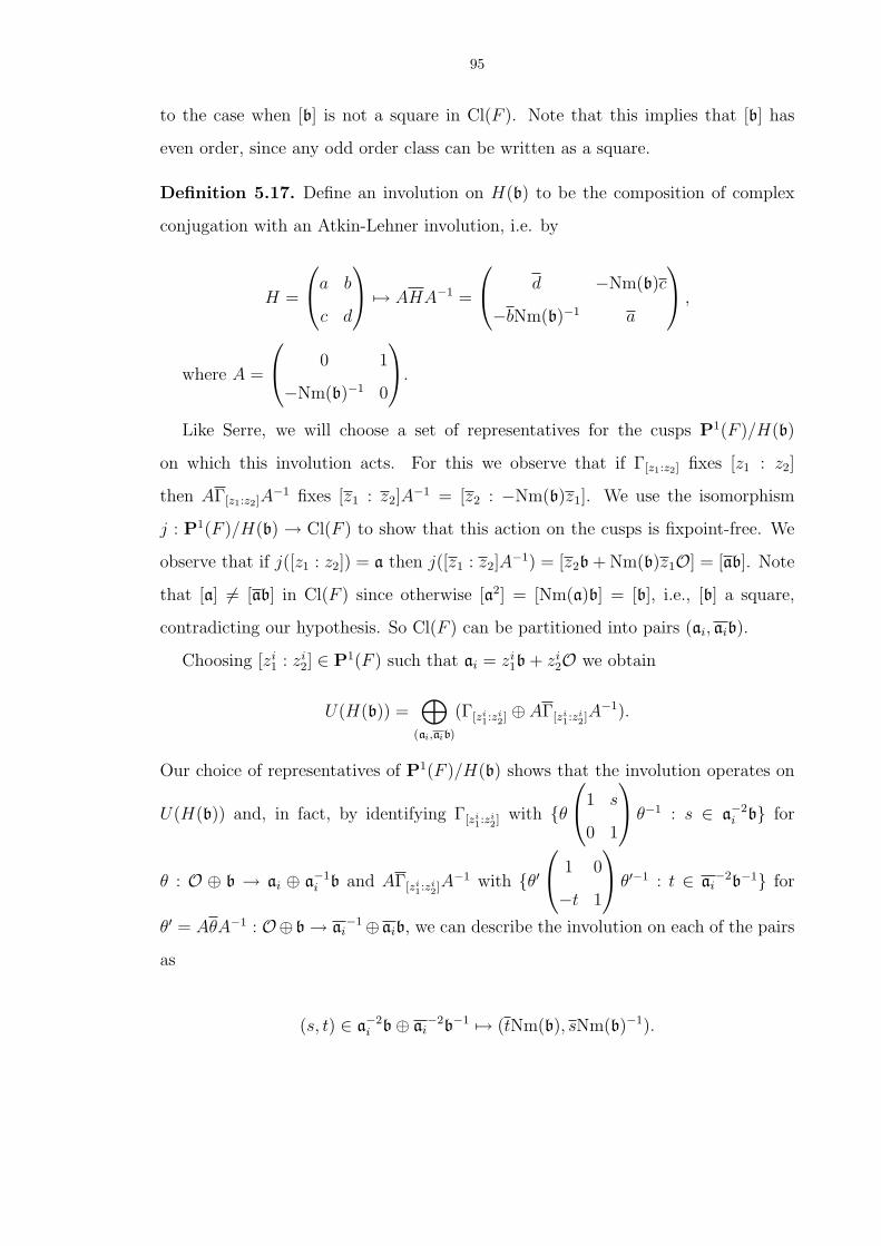
95

to the case when [b] is not a square in Cl(F ). Note that this implies that [b] has

even order, since any odd order class can be written as a square.

Definition 5.17. Define an involution on H(b) to be the composition of complex

conjugation with an Atkin-Lehner involution, i.e. by

H =

a b

c d

7→ AHA−1 =

d −Nm(b)c

−bNm(b)−1 a

,

where A =

0 1

−Nm(b)−1 0

.

Like Serre, we will choose a set of representatives for the cusps P1(F )/H(b)

on which this involution acts. For this we observe that if Γ[z1:z2] fixes [z1 : z2]

then AΓ[z1:z2]A−1 fixes [z1 : z2]A

−1 = [z2 : −Nm(b)z1]. We use the isomorphism

j : P1(F )/H(b) → Cl(F ) to show that this action on the cusps is fixpoint-free. We

observe that if j([z1 : z2]) = a then j([z1 : z2]A−1) = [z2b + Nm(b)z1O] = [ab]. Note

that [a] 6= [ab] in Cl(F ) since otherwise [a2] = [Nm(a)b] = [b], i.e., [b] a square,

contradicting our hypothesis. So Cl(F ) can be partitioned into pairs (ai, aib).

Choosing [zi1 : zi

2] ∈ P1(F ) such that ai = zi1b + zi

2O we obtain

U(H(b)) =⊕

(ai,aib)

(Γ[zi1:zi

2] ⊕ AΓ[zi1:zi

2]A−1).

Our choice of representatives of P1(F )/H(b) shows that the involution operates on

U(H(b)) and, in fact, by identifying Γ[zi1:zi

2] with θ1 s

0 1

θ−1 : s ∈ a−2

i b for

θ : O ⊕ b → ai ⊕ a−1i b and AΓ[zi

1:zi2]A

−1 with θ′ 1 0

−t 1

θ′−1 : t ∈ ai

−2b−1 for

θ′ = AθA−1 : O⊕b → ai−1⊕ aib, we can describe the involution on each of the pairs

as

(s, t) ∈ a−2i b⊕ ai

−2b−1 7→ (tNm(b), sNm(b)−1).

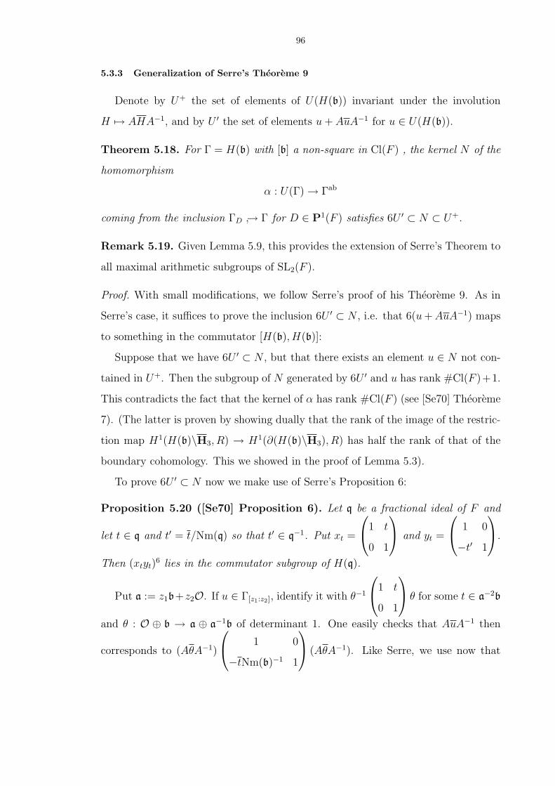
96

5.3.3 Generalization of Serre’s Theoreme 9

Denote by U+ the set of elements of U(H(b)) invariant under the involution

H 7→ AHA−1, and by U ′ the set of elements u + AuA−1 for u ∈ U(H(b)).

Theorem 5.18. For Γ = H(b) with [b] a non-square in Cl(F ) , the kernel N of the

homomorphism

α : U(Γ) → Γab

coming from the inclusion ΓD → Γ for D ∈ P1(F ) satisfies 6U ′ ⊂ N ⊂ U+.

Remark 5.19. Given Lemma 5.9, this provides the extension of Serre’s Theorem to

all maximal arithmetic subgroups of SL2(F ).

Proof. With small modifications, we follow Serre’s proof of his Theoreme 9. As in

Serre’s case, it suffices to prove the inclusion 6U ′ ⊂ N , i.e. that 6(u + AuA−1) maps

to something in the commutator [H(b), H(b)]:

Suppose that we have 6U ′ ⊂ N , but that there exists an element u ∈ N not con-

tained in U+. Then the subgroup of N generated by 6U ′ and u has rank #Cl(F )+1.

This contradicts the fact that the kernel of α has rank #Cl(F ) (see [Se70] Theoreme

7). (The latter is proven by showing dually that the rank of the image of the restric-

tion map H1(H(b)\H3, R) → H1(∂(H(b)\H3), R) has half the rank of that of the

boundary cohomology. This we showed in the proof of Lemma 5.3).

To prove 6U ′ ⊂ N now we make use of Serre’s Proposition 6:

Proposition 5.20 ([Se70] Proposition 6). Let q be a fractional ideal of F and

let t ∈ q and t′ = t/Nm(q) so that t′ ∈ q−1. Put xt =

1 t

0 1

and yt =

1 0

−t′ 1

.

Then (xtyt)6 lies in the commutator subgroup of H(q).

Put a := z1b+z2O. If u ∈ Γ[z1:z2], identify it with θ−1

1 t

0 1

θ for some t ∈ a−2b

and θ : O ⊕ b → a ⊕ a−1b of determinant 1. One easily checks that AuA−1 then

corresponds to (AθA−1)

1 0

−tNm(b)−1 1

(AθA−1). Like Serre, we use now that

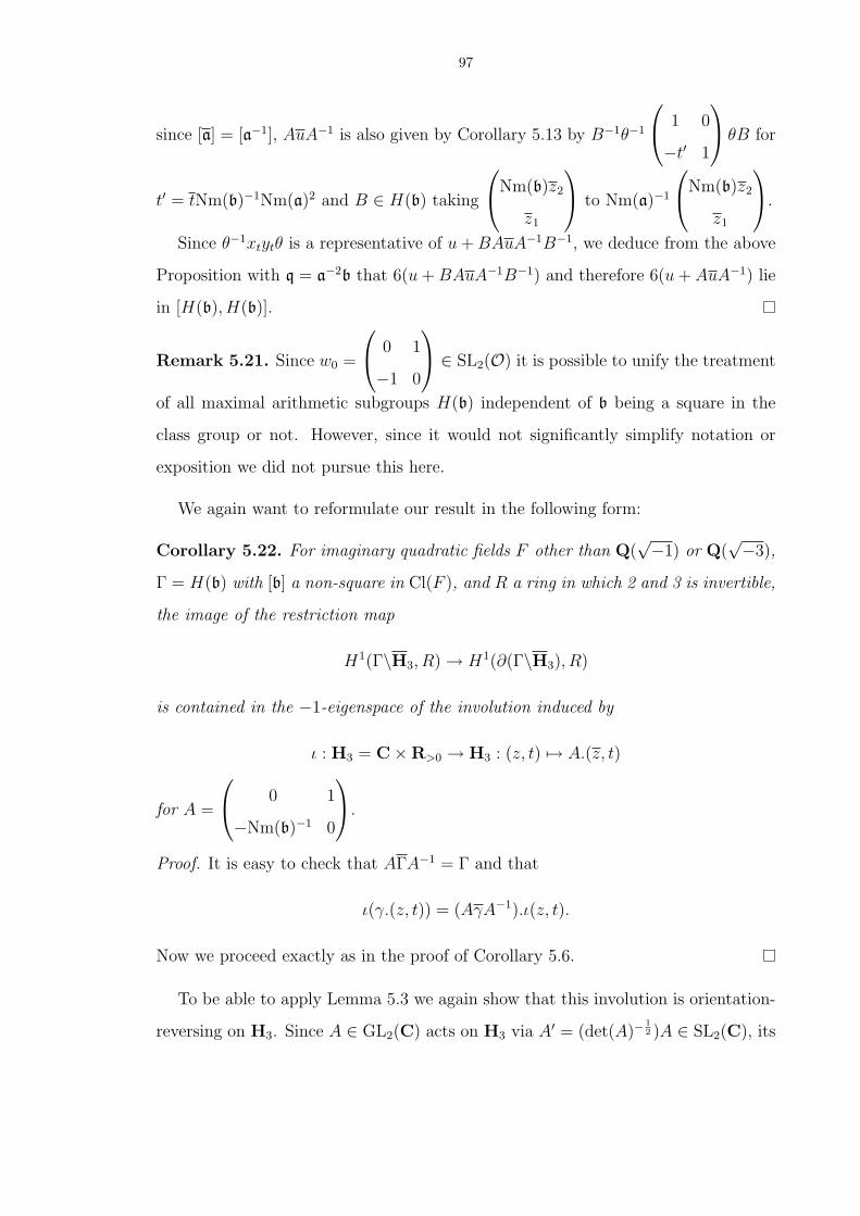
97

since [a] = [a−1], AuA−1 is also given by Corollary 5.13 by B−1θ−1

1 0

−t′ 1

θB for

t′ = tNm(b)−1Nm(a)2 and B ∈ H(b) taking

Nm(b)z2

z1

to Nm(a)−1

Nm(b)z2

z1

.

Since θ−1xtytθ is a representative of u + BAuA−1B−1, we deduce from the above

Proposition with q = a−2b that 6(u + BAuA−1B−1) and therefore 6(u + AuA−1) lie

in [H(b), H(b)].

Remark 5.21. Since w0 =

0 1

−1 0

∈ SL2(O) it is possible to unify the treatment

of all maximal arithmetic subgroups H(b) independent of b being a square in the

class group or not. However, since it would not significantly simplify notation or

exposition we did not pursue this here.

We again want to reformulate our result in the following form:


√−3),

Γ = H(b) with [b] a non-square in Cl(F ), and R a ring in which 2 and 3 is invertible,

the image of the restriction map

H1(Γ\H3, R) → H1(∂(Γ\H3), R)

is contained in the −1-eigenspace of the involution induced by

ι : H3 = C×R>0 → H3 : (z, t) 7→ A.(z, t)

for A =

0 1

−Nm(b)−1 0

.

Proof. It is easy to check that AΓA−1 = Γ and that

ι(γ.(z, t)) = (AγA−1).ι(z, t).

Now we proceed exactly as in the proof of Corollary 5.6.

To be able to apply Lemma 5.3 we again show that this involution is orientation-

reversing on H3. Since A ∈ GL2(C) acts on H3 via A′ = (det(A)−12 )A ∈ SL2(C), its

98

action on H3 preserves the orientation (see end of Section 5.2, before Corollary 5.7).

Recalling further that the action of complex conjugation is orientation-reversing,

our involution is therefore orientation-reversing. For future reference we record the

application of Lemma 5.3 to our involution:


√−3),

Γ = H(b) with [b] a non-square in Cl(F ), and R a complete discrete valuation ring

in which 2 and 3 are invertible and with finite residue field of characteristic p > 2,

the restriction map

H1(Γ\H3, R) → H1(∂(Γ\H3), R)−

surjects onto the −1-eigenspace of the involution induced by

ι : H3 = C×R>0 → H3 : (z, t) 7→ A.(z, t)

for A =

0 1

−Nm(b)−1 0

.

5.4 Unramified characters χ

In Chapter III we defined an Eisenstein cohomology class associated to (µ1, µ2) on

an adelic symmetric space SKsf

for a specific choice of Ksf . In this section we will show

that for unramified characters χ = µ1/µ2 we can always write the corresponding SKsf

as a disjoint union of Γ\H3 with Γ = H(b) for fractional ideals b. This allows us

to apply our results for maximal arithmetic subgroups from the previous sections

by considering the restriction maps to the boundary separately for each connected

component.

We recall now from Section 2.3: The space SKfhas several connected components,

in fact, strong approximation implies that the fibers of the determinant map

SKf= G(Q)\G(A)/(KfK∞) ³ HK := A∗

F /det(K)F ∗

(where K = KfK∞) are connected. Any ξ ∈ G(Af ) gives rise to an injection

jξ : G∞ → G(A) with jξ(g∞) = (g∞, ξ) and, after taking quotients, to a component

Γξ\G∞/K∞ → G(Q)\G(A)/K,

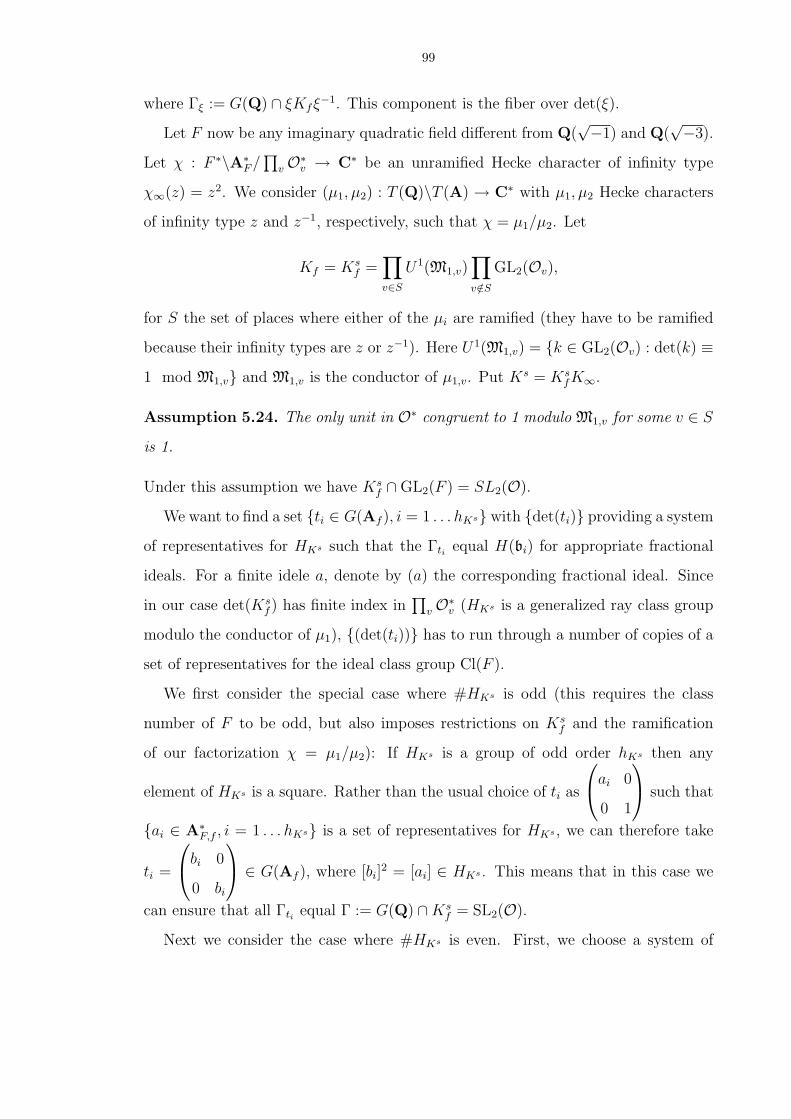
99

where Γξ := G(Q) ∩ ξKfξ−1. This component is the fiber over det(ξ).

Let F now be any imaginary quadratic field different from Q(√−1) and Q(

√−3).

Let χ : F ∗\A∗F /

∏v O∗

v → C∗ be an unramified Hecke character of infinity type

χ∞(z) = z2. We consider (µ1, µ2) : T (Q)\T (A) → C∗ with µ1, µ2 Hecke characters

of infinity type z and z−1, respectively, such that χ = µ1/µ2. Let

Kf = Ksf =

∏v∈S

U1(M1,v)∏

v/∈S

GL2(Ov),

for S the set of places where either of the µi are ramified (they have to be ramified

because their infinity types are z or z−1). Here U1(M1,v) = k ∈ GL2(Ov) : det(k) ≡1 mod M1,v and M1,v is the conductor of µ1,v. Put Ks = Ks

fK∞.

Assumption 5.24. The only unit in O∗ congruent to 1 modulo M1,v for some v ∈ S

is 1.

Under this assumption we have Ksf ∩GL2(F ) = SL2(O).

We want to find a set ti ∈ G(Af ), i = 1 . . . hKs with det(ti) providing a system

of representatives for HKs such that the Γti equal H(bi) for appropriate fractional

ideals. For a finite idele a, denote by (a) the corresponding fractional ideal. Since

in our case det(Ksf ) has finite index in

∏v O∗

v (HKs is a generalized ray class group

modulo the conductor of µ1), (det(ti)) has to run through a number of copies of a

set of representatives for the ideal class group Cl(F ).

We first consider the special case where #HKs is odd (this requires the class

number of F to be odd, but also imposes restrictions on Ksf and the ramification

of our factorization χ = µ1/µ2): If HKs is a group of odd order hKs then any

element of HKs is a square. Rather than the usual choice of ti as

ai 0

0 1

such that

ai ∈ A∗F,f , i = 1 . . . hKs is a set of representatives for HKs , we can therefore take

ti =

bi 0

0 bi

∈ G(Af ), where [bi]

2 = [ai] ∈ HKs . This means that in this case we

can ensure that all Γti equal Γ := G(Q) ∩Ksf = SL2(O).

Next we consider the case where #HKs is even. First, we choose a system of

100

representatives γj of

ker(HKs → Cl(F )) ∼= O∗\∏

v

O∗v/det(Ks

f ).

Then take a set of representatives ak of Cl(F )/(Cl(F ))2 in A∗F,f (represent the

principal ideals by (1)). Lastly, we choose a set b2m representing Cl(F )2.

Now we can define ti as follows: The set is given by the elements

γjakbm 0

0 bm

∈ G(Af ),

as j, k and m run through their indexing sets.

We obtain a decomposition

SKsf

∼=hKs∐i=1

Γti\G∞/K∞ ∼=hKs∐i=1

Γti\H3,

where Γti = G(Q) ∩ tiKsf t−1i , with the i-th connected component Γti\H3 being em-

bedded via jti .

Note that if ti =

γjakbm 0

0 bm

, the associated Γti = H((ak)) under Assumption

5.24. Also, by construction, either ak = 1 or [(ak)] is not a square in Cl(F ).

5.5 Integral lift of constant term

In this section we show that for χ = µ1/µ2 an unramified character we can lift the

constant term of the Eisenstein cohomology class to an integral class, i.e., that there

exists c ∈ H1(SKsf,Oχ) with the same restriction to the boundary as the Eisenstein

cohomology class.

Our setup is as follows: Let F be an imaginary quadratic field, distinct from

Q(√−1) and Q(

√−3). Suppose p is a prime of F such that the underlying rational

prime p is greater than 3 and splits in F .

Let µ1, µ2 : F ∗\A∗F → C∗ be Hecke characters of infinity type z and z−1, re-

spectively, such that χ = µ1/µ2 is unramified. Denote by S the set of places where

101

the µi are ramified. Assume in addition that 1 is the only unit in O∗ congru-

ent to 1 modulo M1,v for some v ∈ S (i.e., that Assumption 5.24 holds). Put

φ = (µ1, µ2) : T (Q)\T (A) → C∗. Let Oχ denote the ring of integers in the finite

extension Fχ of Fp obtained by adjoining the values of both µi,f and Lalg(0, χ).

In the last section we showed that under these conditions there exist ti ∈ G(Af )such that det(ti) is a system of representatives for HKs and such that the Γti are all

either SL2(O) or H(b) for fractional ideals b whose classes are non-square in Cl(F ).

Since unramified characters are anticyclotomic (see Lemma 3.16) Lemma 3.24 applies

so that [res(Eis(ω0(φ, Ψφ)))] is integral. We can further show:

Proposition 5.25.

[res(Eis(Ψφ))] ∈ H1(∂SKsf,Oχ)−,

where the latter is defined via the isomorphism to

⊕

[det(ti)]∈HKs

H1(∂(Γti\H3),Oχ)−

for the choice of ti’s from the last section and where the involutions on each of the

connected components are defined as in Corollaries 5.7 (if Γti = SL2(O)) and 5.23

(if Γti = H(b) for b a non-square in Cl(F )).

Remark 5.26. Together with Corollaries 5.7 and 5.23 this shows the existence of

an integral lift of the constant term. Note that Oχ is the ring of integers in a finite

extension of Fp so that the conditions in these corollaries are satisfied.

Proof. We shorten the notation to

ω0(Ψφ)) := ω0(φ, Ψφ)) and ω0(Ψw0.φ) := ω0(w0.φ, Ψw0.φ).

Under the assumptions in this section we have that

[res(Eis(ω0(Ψφ)))] = [ω0(Ψφ)− ω0(Ψw0.φ)] ∈ H1(∂SKsf,Oχ)

(see the proof of Lemma 3.24). Recall that the boundary of the Borel-Serre com-

pactification of the adelic symmetric space is homotopy equivalent to

∂SGKs

f= B(Q)\G(A)/Ks

fK∞ ∼=⊕

[det(ti)]∈HKs

⊕

[η]∈P1(F )/Γti

Γti,Bη\H3,

102

where Γti,Bη = Γti ∩ η−1B(Q)η for η ∈ G(Q). We will consider the restriction

maps to the boundary separately for each connected component Γti\H3 and use the

isomorphisms with group cohomology:

H1(Γti\H3,Oχ) ∼= H1(Γti ,Oχ)res→ H1(∂(Γti\H3),Oχ) ∼=

⊕

[η]∈P1(F )/Γti

H1(Γti,Bη ,Oχ).

We need to show therefore that the cohomology class determined by the constant

term lies in the −1-eigenspace of the involution induced by u 7→ u for Γti = SL2(O)

and by u 7→ AuA−1 for Γti = H(b).

The restriction to Γti,P\H3 was denoted by [restiP (Eis(ω0(Ψφ)))] and equals, by

Lemma 3.6 and the proof of Lemma 3.24, the class of

ω0(Ψφ)tiP − ω0(Ψw0.φ)ti

P .

For P = Bη the image of the latter under Gη−1∞ K∞ (we will drop the subscript from

now on) was calculated in Lemma 3.10 and is given in our case (when m = n = 0)

by:

G(ω0(Ψφ)tiBη)(η−1

∞

1 x

0 1

η∞) = xΨφ(ηf ti)

G(ω0(Ψw0.φ)tiBη)(η−1

∞

1 x

0 1

η∞) = xΨw0.φ(ηf ti).

Note that by Lemma 5.4 we can restrict to Uη.

Case (1). We again first treat the notationally simpler case where all Γti equal

SL2(O) and the involution is complex conjugation on the matrix entries.

We claim that

G(ω0(Ψφ)tiBη)(g) = G(ω0(Ψw0.φ)

tiBη)(g) for all g ∈ Γti,Uη .

Given the form of the constant term this immediately implies that it lies in the −1

eigenspace for the involution induced by complex conjugation.

Recall that in this case ti =

γibi 0

0 bi

for some γi ∈ O∗ and bi ∈ A∗

F,f . We will

also use that the Ψφ (which were defined in Section 3.2 as a product of local factors)

103

satisfy

Ψφ(

a b

0 d

k) = µ1(a)µ2(d) for

a b

0 d

∈ B(A), k ∈

∏v

SL2(Ov) ⊂ Ksf .

Note that, in particular, Ψφ(bg) = φ−1∞ (b)Ψφ(g) for b ∈ B(F ) ⊂ G(Af ).

We are therefore left to show that Ψφ(ηf ti) = Ψw0.φ(ηf ti). For this we use the

Bruhat decomposition of matrices in GL2(F ) given by:

(5.1)

a b

c d

=

1 b/d

0 1

a 0

0 d

if c = 0,

1 a/c

0 1

ad−bcc

0

0 −c

0 1

−1 0

1 d/c

0 1

otherwise.

Since Ψφ(

a b

0 d

g) = Ψφ(

a b

0 d

)Ψφ(g) we can consider separately the cases

(a) η =

a b

0 d

for a, b, d ∈ F and

(b) η =

0 1

−1 0

1 e

0 1

for e ∈ F .

We check that for (a)

Ψφ(ηf

γibi 0

0 bi

) = µ1(γibi)µ2(bi)Ψφ(ηf )

and

Ψw0.φ(ηf

γibi 0

0 bi

) = µ2(γi)|γi|µ1(bi)µ2(bi)Ψw0.φ(ηf ).

Since γi ∈ O∗ and χ = µ1/µ2 is unramified it suffices to show that Ψφ(ηf ) =

Ψw0.φ(ηf ). In case (b) we similarly reduce to this assertion.

In (a) we get Ψφ(ηf ) = µ−11,∞(a)µ−1

2,∞(d) = da. Since w0.φ has infinity type (z, z−1)

this equals Ψw0.φ(ηf ). In (b) we need to calculate the Iwasawa decomposition of η in

104

GL2(Fv) if e /∈ Ov (at all other places Ψφ(ηv) = Ψw0.φ(ηv) = 1). It is given by 0 1

−1 0

1 e

0 1

=

e−1 0

0 e

−1 0

−e−1 −1

.

So, if e /∈ Ov then Ψφ(ηv) = (µ2/µ1)v(e) = χ−1v (e), which we claim matches

Ψw0.φ(ηv) = (µ1/µ2)v(e)|e|−2v . This follows from χc = χ and χχ = | · |2 (for the

latter see Lemma 3.14).

Case (2). We now treat the case of Γti = H(b), where the involution is induced

by H 7→ AHA−1 for A =

0 1

−N−1 0

with N = Nm(b). Considering the effect of

the involution on the cusp corresponding to Bη, we claim that

G(ω0(Ψφ)tiBη)(g) = G(ω0(Ψw0.φ)

tiBηA−1 )(AgA−1) for all g ∈ Γti,Uη .

Recall that ti =

xibi 0

0 bi

for some xi, bi ∈ A∗

F,f . We have to show that

(5.2) Ψφ(ηf ti) = Ψw0.φ(ηfA−1ti).

Again making use of the Bruhat decomposition, we need to only consider η as in

cases (a) and (b) above. Following the arguments used for Case (1), Case(a) re-

duces immediately to showing that Ψφ(ti) = Ψw0.φ(A−1ti). The left hand side equals

µ1,f (xibi)µ2,f (bi), the right hand side is

Ψw0.φ(

N 0

0 1

0 1

−1 0

xibi 0

0 bi

) = N−1Ψw0.φ(

bi 0

0 xibi

)

= N−1µ1,f (xibi)µ2,f (bi)|xi|−1f .

Equality follows from |xi|−1f = Nm(b).

For (b), one quickly checks that for η =

0 1

−1 0

the two sides in (5.2) agree.

For the general η =

0 1

−1 0

1 e

0 1

one shows that, on the one hand,

ηf

xibi 0

0 bi

=

bi 0

0 xibi

0 1

−1 0

1 exi

0 1

,

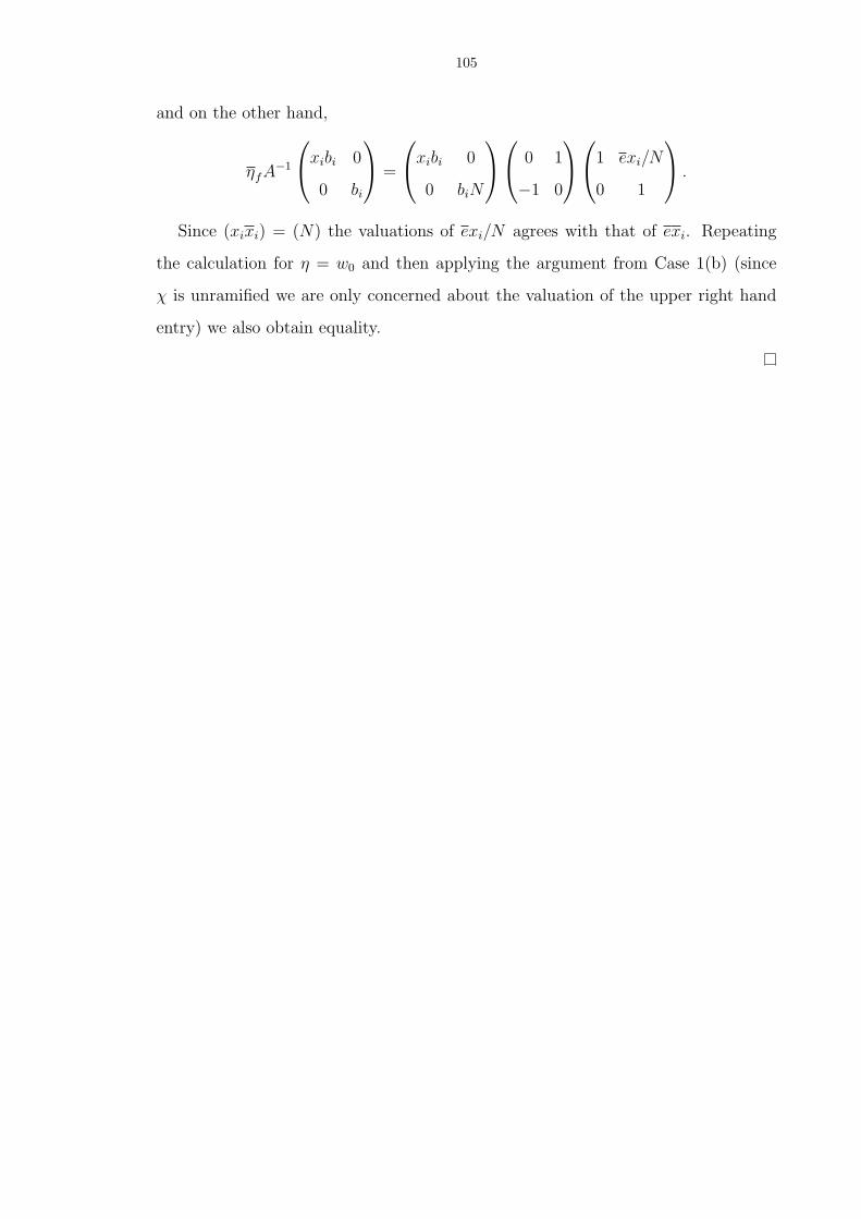
105

and on the other hand,

ηfA−1

xibi 0

0 bi

=

xibi 0

0 biN

0 1

−1 0

1 exi/N

0 1

.

Since (xixi) = (N) the valuations of exi/N agrees with that of exi. Repeating

the calculation for η = w0 and then applying the argument from Case 1(b) (since

χ is unramified we are only concerned about the valuation of the upper right hand

entry) we also obtain equality.

CHAPTER VI

Bounding the Eisenstein ideal

After defining an Eisenstein ideal in a Hecke algebra acting on cohomological

cuspidal automorphic forms, we put the results of Chapters III-V together to prove

a bound for its index in terms of a special L-value.

Recall our setup: Let F be an imaginary quadratic field, distinct from Q(√−1)

and Q(√−3). Suppose p is a prime of F such that the underlying rational prime p

is greater than 3 and splits in F .

We consider unramified Hecke characters χ : F ∗\A∗F → C∗ of infinity type z2

(i.e. χ∞(z) = z2). We gave examples of such characters in Section 3.5 and showed

that they are anticyclotomic, meaning that they satisfy χc = χ. In Corollary 4.18

we obtained characters µ1, µ2 : F ∗\A∗F → C∗ of infinity type z and z−1, respectively,

such that χ = µ1/µ2, for which we could bound from below the denominator of the

Eisenstein cohomology class

[Eis(ω0(φ, Ψφ))] ∈ H1(SKsf, Fχ),

where φ = (µ1, µ2) : T (Q)\T (A) → C∗. For the definition of Eis(ω0(φ, Ψφ)) and Ksf

see Sections 3.2 and 3.3. We recall that Fχ is the finite extension of Fp obtained by

adjoining the values of the finite part of both µi and Lalg(0, χ) (cf. Theorem 2.1) and

that we call its ring of integers Oχ. The choice of characters in the proof of Corollary

4.18 is µ1 = χ·µG and µ2 = µG, where µG is Greenberg’s character from Lemma 3.18.

The character µG has conductor (from now on denoted by M1) divisible precisely by

106

107

the primes ramified in F , and at these primes its restriction to the local units has

order 2. This also ensures that 1 is the only unit in O∗ congruent to 1 modulo the

conductors of µi, so that Ksf ∩ G(Q) = SL2(O) (cf. Assumption 5.24). We denote

by S the set of places where µG is ramified.

6.1 Diamond operators

We assume now in addition that p does not divide #Cl(F ). Let H be the p-Sylow

subgroup of the ray class group ClM1(F ) ∼= F ∗\A∗F /C∗U(M1). Since p does not

divide the class number of F we have

(6.1) H ∼=∏v∈S

Hv ⊂∏v∈S

O∗v/(1 + M1,v) ∼= (O/M1)

∗

for Hv the p-Sylow subgroups of O∗v/(1+M1,v). We define a compact open subgroup

KH,sf containing Ks

f by

KH,sf :=

∏

v/∈S

GL2(Ov)∏v∈S

UHv(M1,v),

where

UHv(M1,v) = k ∈ GL2(Ov) : det(k) ∈ Hv mod M1,v.

Since the spherical vector Ψ0φv

defined in (3.3) is right-invariant under UHv(M1,v)

due to µ1,v|O∗v having order 2 we see that ω0(φ, Ψφ) also defines a nontrivial class in

H1(∂SKH,sf

,Oχ) for the slightly larger group KH,sf (cf. the corresponding statement

for Ksf in Proposition 3.23) and Eis(ω0(φ, Ψφ)) defines a class in H1(SKH,s

f, Fχ) which

we will denote by cχ. Our arguments in chapters III-V apply to KH,sf and this

particular character φ = (χ · µG, µG) without change. Note, in particular, that

KH,sf ∩G(Q) = SL2(O) also, since −1 /∈ H (cf. Section 5.4).

By [U98] §1.2 and §1.4.5 we have for any O-algebra R an R-linear action of the

ray class group ClM1(F ) on H1(SKH,sf

, R) via the diamond operators (see Section

2.9.2). For a prime ideal q not dividing M1 the action of [q] ∈ ClM1(F ) is given by

the Hecke operator

Sv = [KH,sf

πv 0

0 πv

KH,s

f ]

108

for v the place corresponding to q and πv a uniformizer of Ov. This uses that

KH,sf ⊃ K(M1) :=

a b

c d

∈ K0

f :

a b

c d

≡

1 0

0 1

mod M1

.

We claim that the action of the diamond operators Sv, v /∈ S, is trivial if [(πv)] ∈H ⊂ ClM1(F ) (recall that we use the notation (g) for the fractional ideal generated

by a finite idele g). By (6.1) we have [(πv)] = [αO] for some α ∈ O with α ∈ H

mod M1. Therefore Sv has the same action as [KH,sf

α′ 0

0 α′

KH,s

f ] for α′ ∈ A∗F an

idele with (α′f ) = αO and α′v = 1 for each v ∈ S and v = ∞. But

α′ 0

0 α′

∈ G(A)

can be written as the product of

α 0

0 α

∈ Z(Q) → G(A) and an element of

Z∞ ·KH,sf and so its Hecke action is trivial.

We conclude that we have an action of Oχ[ClM1(F )/H] on H1(SKH,sf

, R) for any

Oχ-algebra R. Since ClM1(F )/H has order prime to p, Oχ[ClM1(F )/H] is semisimple.

For ω := µ1µ2, which can be viewed as a character of ClM1(F )/H, let eω be the

idempotent associated to ω−1, so that Sveω = ω(πv)−1eω. For R = C the idempotent

eω projects to cuspforms with central character ω via the Eichler-Shimura-Harder

isomorphism.

6.2 Main result

Recall that H i! (SKH,s

f, R) := im(H1

c (SKH,sf

, R) → H1(SKH,sf

, R)) for any Oχ-algebra

R and that H1! (SKH,s

f,Oχ) := im(H1

! (SKH,sf

,Oχ) → H1! (SKH,s

f, Fχ)).

Definition 6.1. Denote by Tχ the Oχ-subalgebra of EndOχ(eωH1! (SKH,s

f,Oχ)) gen-

erated by the Hecke operators Tv = [KH,sf

1 0

0 πv

KH,s

f ] for all primes v /∈ S.

109

Definition 6.2 (Eisenstein ideal). We call the ideal Iµ1,µ2 ⊆ Tχ generated by

Tv − µ−1

1,v(Pv)− µ−12,v(Pv)Nm(Pv)|v /∈ S

the Eisenstein ideal associated to (µ1, µ2). Here Pv is the maximal ideal in Ov.

Our main result can now be stated as:

Theorem 6.3. There is an Oχ-algebra surjection

Tχ/Iµ1,µ2 ³ Oχ/(Lalg(0, χ)

).

Proof. Recall the long exact sequence

. . . → H1c (SKH,s

f, R) → H1(SKH,s

f, R)

res−→ H1(∂SKH,sf

, R) → H2c (SKH,s

f, R) → . . .

for any Oχ-algebra R. The class cχ ∈ H1(SKH,sf

, Fχ) is annihilated by Tv−µ−11,v(Pv)−

µ−12,v(Pv)Nm(Pv), v /∈ S (cf. Lemma 3.11). Since χc = χ, its (non-trivial) restriction

to the boundary res(cχ) lies in H1(∂SKH,sf

,Oχ) (cf. Lemma 3.24). In Corollary

4.18 we showed that the denominator of cχ is bounded below by Lalg(0, χ) (i.e.,

δ(cχ) ⊂ (Lalg(0, χ)). In Chapter V, we proved that there exists c ∈ H1(SKH,sf

,Oχ)

with the same restriction to the boundary as the Eisenstein cohomology class cχ.

Note that

res(eωc) = eωres(c) = eωres(cχ) = res(cχ)

since

Sv(cχ) = ω−1(πv)cχ.

We can now prove the theorem following the proof of Proposition 6.2 in [S02a]:

Without loss of generality, we can assume that δ(cχ) ( Oχ; there is nothing to prove

otherwise. Let δ be a generator of δ(cχ). Then δcχ is an element of an Oχ-basis of

eωH1(SKH,sf

,Oχ). By construction, c0 := δ ·(eωc−cχ) ∈ H1! (SKH,s

f,Oχ) is a nontrivial

element of an Oχ-basis of eωH1! (SKH,s

f,Oχ). Extend c0 to an Oχ-basis c0, c1, . . . cd of

H1! (SKH,s

f,Oχ). For each t ∈ Tχ write

t(c0) =d∑

i=0

ai(t)ci, ai(t) ∈ Oχ.

110

Then

(6.2) Tχ → Oχ/(δ), t 7→ a0(t) mod δ

is an Oχ-module surjection. We claim that it is independent of the Oχ-basis chosen

and that it is a homomorphism of Oχ-algebras with the Eisenstein ideal Iµ1,µ2 con-

tained in its kernel. To prove this it suffices to check that each a0(Tv − µ−11,v(Pv) −

Nm(Pv)µ−12,v(Pv)), v /∈ S is contained in δOχ. This is an easy calculation. Let

tv = Tv − µ−11,v(Pv) − Nm(Pv)µ

−12,v(Pv). Then by Lemma 3.11, tvcχ = 0 and hence

tvc0 = tvδeωc ∈ δH1! (SKH,s

f,Oχ). Thus a0(tv) ∈ δOχ and (6.2) is a well-defined Oχ-

algebra surjection, coinciding with Tv 7→ µ−11,v(Pv) + Nm(Pv)µ

−12,v(Pv) mod δ. Since

Oχ/(δ) ³ Oχ/(Lalg(0, χ)) by Corollary 4.18, this proves our theorem.

Remark 6.4. 1. Note that the right-hand side in the statement of the theorem

is nontrivial if p divides Lalg(0, χ). If the left-hand side Tχ/Iµ1,µ2 is non-trivial

then a minimal prime contained in Iµ1,µ2 gives rise (via the Eichler-Shimura-Harder

isomorphism) to a cuspidal eigenform with eigenvalues congruent to those of the

Eisenstein cohomology class. Using the same notation as in the proof, the class

c ∈ H1(SKH,sf

,Oχ) exhibits a non-trivial element of the cohomological congruence

module M/(N ⊕N ′) for M = H1(SKH,sf

,Oχ), N = H1! (SKH,s

f,Oχ), and N ′ = δcχOχ.

See [P] and [Gh] for more details on congruence modules and their relationships.

2. L(0, χ) 6= 0 since 0 is the abscissa of convergence for this (non-unitary) infinity

type (see [La] XV §4).

3. Observe that for Q(√−1) and Q(

√−3) (the fields excluded above) the bound-

ary cohomology for constant coefficients and maximal compact open subgroups Kf

is trivial.

CHAPTER VII

Application to bounding Selmer groups

In this chapter we will demonstrate how to apply Theorem 6.3 to bound the size

of certain Selmer groups from below by Lalg(0, χ).

7.1 Background

We keep the following notation from the previous Chapter: p, F , p, χ, Fχ, Oχ.

Let R be the integer ring in a finite extension L of Fp. Denote its maximal ideal

by mR. Let GF := Gal(F/F ), and for Σ a finite set of places of F containing the

places above p let GΣ be the Galois group of the maximal extension of F unramified

at all places not in Σ. For any place v of F , Gv and Iv denote, respectively, the

decomposition group and the inertia subgroup for v determined by F → F v. Denote

by χp the infinite order p-adic Galois character associated to χ (see end of Section

2.6) and by ε : GF → Z∗p the p-adic cyclotomic character defined by the action of GF

on the p-power roots of unity: g.ξ = ξε(g) for ξ with ξpm= 1 for some m.

7.1.1 Fitting ideals

We recall the definition and basic properties of Fitting ideals. For details we refer

to the Appendix of [MW]. Let A be a ring and let M be a finitely generated A-module

with generators m1, . . . , mn. Let f : An ³ M be the surjective A-homomorphism

defined by f(ei) = mi for i = 1, . . . , n. Here ei denotes the ith standard basis vector

of An. The Fitting ideal FittA(M) of M is the ideal generated by the determinants

111

112

det(v1, . . . , vn) for which the column vectors v1, . . . , vn lie in ker(f). One checks that

this does not depend on the choice of the generators mi.

The following proposition contains the properties of the Fitting ideal that we will

use:

Proposition 7.1. (i) FittA(M) ⊂ AnnA(M).

(ii) For any A-algebra B we have FittB(M ⊗A B) = FittA(M) ·B.

(iii) For any ideal a ⊂ A we have FittA(A/a) = a.

(iv) If A is a complete local Noetherian ring with maximal ideal mA and M an

A-module of finite length, then

mlengthA(M)A ⊂ FittA(M).

Remark 7.2. For rings A that are complete discrete valuation rings of residue char-

acteristic p (like Oχ or R) we will write valp(#M) instead of lengthA(M).

7.1.2 Galois cohomology

For any profinite group G (e.g. GF or GΣ) call N a topological G-module if it is a

commutative topological group with a continuous action of G. Given a topological G-

module N , define the continuous cohomology groups H i(G,N) to be the cohomology

of the complex defined by continuous cochains (for details see [Ru] Appendix B.2):

Let Ci(G,N) = f : Gi → N continuous . For every i ≥ 0 there is a coboundary

map di : Ci(G,N) → Ci+1(G,N) and we set H1(G,N) := ker(di)/image(di−1). The

group H0(G,N) can be identified with NG, and for the trivial G-action on N we have

H1(G,N) = Homcts(G,N). Note also that for discrete modules any homomorphism

is continuous.

When N has the additional structure of an S-module for some ring S and the

G-action is S-linear (call this an S[G]-module), the continuous cohomology groups

are S-modules.

If 0 → T ′ → T → T ′′ → 0 is an exact sequence of topological S[G]-modules and

if there exists a continuous section (a map of sets, not necessarily a homomorphism)

113

from T ′′ → T , then we call it a topological short exact sequence (cf. [Ru] Appendix

B.2, [BW] p. 258).

Proposition 7.3. If N is a topological S[G]-module, then H1(G,N) classifies (iso-

morphism classes of) topological short exact sequences (of S[G]-modules)

0 → N → E → 1 → 0,

i.e., continuous extension classes of 1 by N , where 1 is the trivial linear representa-

tion of G on S (or S/I for some ideal I).

Proof. Given an extension

0 → Nf→ E

g→ 1 → 0

let e ∈ E project onto an S-generator of 1. Define a 1-cocycle c : G → N by

c(σ) = f−1(e− σ(e)). Since E is a continuous extension, c is a continuous 1-cocycle.

Two isomorphic extensions give rise to the same cohomology class. Note that, in

particular, if E is a split extension, i.e., if there exists a G-invariant continuous section

h such that g h = id1, then this construction yields a 1-coboundary. Furthermore,

if two extensions give rise to the same cohomology class they are isomorphic (see

argument in [Wa] Proposition 4).

Conversely, given a continuous 1-cocycle c : G → N let E be the S-module N⊕S,

where the action of G on N is extended by σ.r = rc(σ) ⊕ r for r ∈ S. Since c is

continuous this gives a topological S[G]-module. We note that if c is a 1-coboundary,

i.e., of the form σ 7→ σ(n)−n for some n ∈ N then r ∈ S 7→ (−rn, r) ∈ N ⊕S splits

the extension E = N ⊕ S.

7.1.3 Selmer groups

Selmer groups are generalizations of the ideal class groups of number fields. To

motivate the general definition of a Selmer group we recall the connection of class

groups with Galois groups via class field theory:

Example 7.4. By class field theory we have a canonical identification of the ideal

class group Cl(F ) with the Galois group of the maximal everywhere unramified

114

abelian extension of F , the Hilbert class field HF . The latter is the quotient of the

Galois group of the maximal abelian extension F ab over F by the images of all the

inertia groups.

If we are just interested in the p-Sylow subgroup Cl(F )[p∞], we can recover this

from Hom(Gal(HF /F ),Qp/Zp) by taking the Pontryagin dual Hom(·,Qp/Zp). But

Hom(Gal(HF /F ),Qp/Zp) can be identified with

ker(H1(GF ,Qp/Zp) →∏

v

H1(Iv,Qp/Zp)).

This will turn out to be the Selmer group for GF of the trivial Galois representation

Zp.

Definition 7.5 (Pontryagin dual). For a topological R-module N put N∨ =

Homcts(N,Qp/Zp). The group N∨ is an R-module via r.f(n) = f(rn), r ∈ R, f ∈N∨, n ∈ N .

Lemma 7.6. If N is a finite R-module, then

HomR(N,R∨) ∼= N∨, f 7→ (n 7→ f(n)(1)),

is an isomorphism of R-modules.

Proof. (This is Lemma 6.1.1(ii)) from [S04].) Observe that R∨ = ∪R∨[mnR]. Since

N is a finite R-module it follows that given f ∈ HomR(N, R∨) there is an n such

that im(f) ∈ R∨[mnR]. Thus the map in the lemma takes values in N∨ (and not just

Hom(N,Qp/Zp)). It is then easy to check that the map

N∨ → HomR(N, R∨), f 7→ (n 7→ (r 7→ f(rn))),

and the map in the lemma are inverses of each other.

By an R-lattice in a finite-dimensional L-space V we mean a finite R-submodule

M ⊂ V that spans V over L.

We define the Selmer group for a “p-ordinary Galois representation” following

Greenberg (cf. [G89]): Suppose given an n-dimensional L-space V and a continuous

115

representation ρ : GΣ → AutL(V ), i.e., such that there exists a GΣ-stable R-lattice

M ⊂ V on which GΣ acts continuously with respect to the mR-adic topology. Suppose

also given a Gw-stable subspace V +w for each place w of F lying over p.

Let M ⊂ V be any GΣ-stable R-lattice. For each w|p let M+w = M ∩V +

w . This is a

Gw-stable R-lattice in V +w . The module M∗ = M ⊗R R∨ is a discrete R[GΣ]-module

and for w|p the module M+,∗w := M+

w ⊗R R∨ is a discrete R[Gw]-module. Moreover,

there are canonical maps M+,∗w → M∗ coming from the inclusions M+

w → M . For

each finite set Σ′ ⊂ Σ\w|p we define a Selmer group associated to M by

Definition 7.7.

Sel(Σ′,M) = ker(H1(GΣ,M∗) → ⊕w|pH1(Iw,M∗/M+,∗

w )⊕w∈Σ′ H1(Iw,M∗)).

We write Sel(M) for Sel(∅,M).

Lemma 7.8. The Pontryagin dual of Sel(T,M) is a finitely generated R-module.

References. [S04] Corollary 6.1.4, [Ru3] Lemma 1.5.7(iii).

Definition 7.9. Suppose ρ : GΣ → R∗ is a continuous Galois character for some Σ

as above. Denote by R(ρ) the free rank one R-module on which GΣ acts via ρ.

We will apply the Selmer group definition in the case of 1-dimensional Galois

characters arising from Hecke characters of type (A0):

Example 7.10. For λ : F ∗\AF → C∗ a Hecke character of type (A0), i.e., with

infinity type zazb with a, b ∈ Z, we associated at the end of Section 2.6 a Galois

character

λp : GabΣ → O∗

λ,

where Σ consists of the places dividing the conductor fλ and the places dividing p,

and Oλ is the ring of integers in the finite extension Fλ of Fp containing the values of

λf . Extending λp trivially to GΣ we put M = Oλ(λp) and V = Fλ(λp) := M ⊗OλFλ.

By definition λp is “locally algebraic”, i.e., for each w|p and u ∈ O∗w with u ≡ 1

mod fλOw we have λp(rec(u)) = uaub, where rec is the Artin reciprocity map. By a

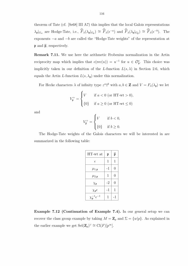
116

theorem of Tate (cf. [Se68] III A7) this implies that the local Galois representations

λp|Gw are Hodge-Tate, i.e., F λ(λp|Gp)∼= F λ(ε

−a) and F λ(λp|Gp) ∼= F λ(ε

−b). The

exponents −a and −b are called the “Hodge-Tate weights” of the representation at

p and p, respectively.

Remark 7.11. We use here the arithmetic Frobenius normalization in the Artin

reciprocity map which implies that ε(rec(u)) = u−1 for u ∈ O∗p. This choice was

implicitly taken in our definition of the L-function L(s, λ) in Section 2.6, which

equals the Artin L-function L(s, λp) under this normalization.

For Hecke characters λ of infinity type zazb with a, b ∈ Z and V = Fλ(λp) we let

V +p =

V if a < 0 (or HT-wt > 0),

0 if a ≥ 0 (or HT-wt ≤ 0)

and

V +p =

V if b < 0,

0 if b ≥ 0.

The Hodge-Tate weights of the Galois characters we will be interested in are

summarized in the following table:

HT-wt at p p

ε 1 1

µ1,p -1 0

µ2,p 1 0

χp -2 0

χpε -1 1

χ−1p ε−1 1 -1

Example 7.12 (Continuation of Example 7.4). In our general setup we can

recover the class group example by taking M = Zp and Σ = w|p. As explained in

the earlier example we get Sel(Zp)∨ ∼= Cl(F )[p∞].

117

For a finite extension K over F the Galois group Gal(K/F ) acts on Cl(K). If we

want to study this finer structure, we can do the following: Let χ : ∆ = Gal(K/F ) →R∗ be a finite order character, with K an abelian extension of F of degree prime to

p. For a Zp[∆]-module B (e.g. Cl(K)[p∞]) denote by Bχ the χ-isotypical piece, i.e.

Bχ := b ∈ B ⊗Zp R : γ.b = χ(γ)b for every γ ∈ ∆. Take Σ sufficiently large such

that ∆ is a quotient of GΣ and extend χ trivially to GΣ. We claim that

Sel(Σ\w|p, R(χ))∨ ∼= Cl(K)[p∞]χ.

This can be seen as follows: In our general notation we have M = R(χ) and

Σ′ = Σ\w|p. Since χ has finite order, its Hodge-Tate weight is 0 and M+w = 0 for

all w|p. Therefore, by definition

Sel(Σ′, R(χ)) = ker(H1(GF ,M∗) →∏

v

H1(Iv,M∗)).

Since [K : F ] is prime to p the inflation-restriction sequence (see [Ru] Prop. B.2.5)

implies that H1(GF ,M∗) ∼= H1(GK ,M∗)∆. Together this shows that Sel(Σ′, R(χ)) =

Hom(Gal(HK/K),M∗)∆ = Hom(Cl(K)[p∞]χ, R∨) for the Hilbert class field HK of

K. The claim follows together with Lemma 7.6.

Definition 7.13. A Galois character ρ : GF → R∗ is called anticyclotomic if it

satisfies ρc = ρ−1, where ρc(σ) = ρ(cσc−1) with c ∈ GQ a lift of the non-trivial

automorphism of Gal(F/Q).

Example 7.14. If λ : F ∗\A∗F → C∗ is an anticyclotomic unitary Hecke character

(i.e. λc = λ = λ−1), then λp is anticyclotomic.

Lemma 7.15. We have Sel(ρ) ∼= Sel(ρc). Here the isomorphism is induced by con-

jugation of GF by a lift of the non-trivial automorphism of Gal(F/Q).

7.2 Statement and discussion of result

Let Σ0 be the set comprising the places above p and the places ramified in F/Q.

Using a method developed by Wiles, Skinner, and Urban, we will prove:

118

Proposition 7.16. With the same assumptions and notation as Theorem 6.3 and

Σ = Σ0, we have

valp(#Sel(M)∨) ≥ valp(#(Tχ/Iµ1,µ2))

for either M = Oχ(χpε) or M = Oχ((χpε)c) = Oχ(χ−1

p ε−1) (the two Selmer groups

are isomorphic by Lemma 7.15).

Remark 7.17. Note that χpε has negative Hodge-Tate weight at the place p and

positive at the place p, so Sel(Oχ(χpε)) will consist of cohomology classes unramified

at p, but possibly ramified at p.

Using Theorem 6.3, this immediately gives us lower bounds on the size of the

Selmer groups in terms of the special L-value:

Corollary 7.18. With the same assumptions and notation as Theorem 6.3 and Σ =

Σ0, we have

valp(#Sel(M)∨) ≥ valp(#(Oχ/(Lalg(0, χ))))

for M = Oχ(χpε) or M = Oχ((χpε)c) = Oχ(χ−1

p ε−1).

Remark 7.19. That Lalg(0, χ) gives bounds for these two Selmer groups is related

(via the anticyclotomic main conjecture) to the fact that Lalg(0, χ) gets interpolated

by two p-adic L-functions, see [AH] p. 12. See Remark 7.35 for the relation of our

results to consequences of the Main Conjecture of Iwasawa theory.

7.3 Proof of Proposition 7.16

We need to procure the ingredients of the following proposition, adapted for our

purposes from [S04] Proposition 6.1.17:

Proposition 7.20. Let ρ : GΣ → O∗χ be a continuous 1-dimensional representation

with positive Hodge-Tate weight at one of the primes lying above p, negative at the

other (call the latter prime w). Denote the module by M and write ρ for the reduction

modulo the maximal ideal of Oχ. Let T be a finite Oχ-algebra and I ⊂ T an ideal

such that the Oχ-algebra structure map surjects onto T/I.

119

Suppose we are given:

• a finite T -module L on which GΣ acts continuously and T -linearly and having

no T [GΣ] -quotient isomorphic to ρ.

• a T [GΣ]-submodule L1 ⊂ L such that GΣ acts trivially on L/L1 and L/L1∼=

T/I.

• a finite T -module T with FittT (T ) ⊂ I ⊂ AnnT (T ) and a T [GΣ]-identification

L1∼= M ⊗Oχ T .

We further require that the T [GΣ]-extension

0 → L1 → L → L/L1 → 0

be split when viewed as a T [Iw]-extension. Given this set-up,

valp(#Sel(M)∨) ≥ valp(#(T/I)).

Proof. We redo the proof of [S04] in our special case. As in Proposition 7.3 we fix

e ∈ L projecting onto a T -generator of L/L1 and define a 1-cocycle c : GΣ → M ⊗Tby

c(σ) = the image of e− σ(e) in L1.

Consider the Oχ-homomorphism

φ : HomOχ(T ,O∨χ) → H1(GΣ,M ⊗O∨

χ), φ(f) = the class of (1⊗ f) c.

We will show that

(i) im(φ) ⊂ Sel(M),

(ii) ker(φ)∨ = 0.

From (i) it follows that

valp(#Sel(M)∨) ≥ valp(#im(φ)∨).

120

From (ii) it follows that

valp(#im(φ)∨) ≥ valp(#Hom(HomOχ(T ,O∨χ),Qp/Zp))

= valp(#Hom(T ∨,Qp/Zp))

= valp(#T )

≥ valp(#T/I),

where the first equality comes from Lemma 7.6, and the last inequality from our

assumption on T and Proposition 7.1(iv). The latter implies that lengthT (T ) ≥lengthT (T/I). Since the action of T on both T and T/I is via T/I, which is a

quotient of Oχ, any Oχ-submodule of T or T/I is, in fact, a T -submodule. This

implies the corresponding inequality for the Oχ-lengths.

For (i) we observe that the assumption that the extension splits when considered

as an extension of T [Iw]-modules implies by Proposition 7.3 that the class cw in

H1(Iw,L1) determined by c is the zero class. This shows that im(φ) ⊂ Sel(M).

To prove (ii) we first observe that for any f ∈ HomOχ(T ,O∨χ), ker(f) has finite

index in T (like in the proof of Lemma 7.6 we see that f ∈ HomOχ(T ,O∨χ [pn]) for

some n). Suppose now that f ∈ ker(φ). We claim that the class of c in H1(GΣ, M⊗Oχ

T /ker(f)) is zero. To see this, let X = O∨χ/im(f) and observe that there is an exact

sequence

H0(GΣ,M ⊗Oχ X) → H1(GΣ,M ⊗Oχ T /ker(f)) → H1(GΣ,M ⊗Oχ O∨χ).

Since f ∈ ker(φ) and the second arrow in the sequence comes from the inclusion

T /ker(φ) → O∨χ induced by f , the image in the right module of the class of c in

the middle is zero. Our claim follows therefore if the module on the left is trivial.

But the dual of this module is a subquotient of HomOχ(M,Oχ) on which GΣ acts

trivially. By assumption, however, M has no nontrivial subquotients.

Suppose in addition that f is non-trivial, i.e. ker(f) ( T . Then there exists a

T -module A with ker(f) ⊂ A ⊂ T such that T /A ∼= Oχ/p (we use here again that

121

any Oχ-submodule of T is actually a T -submodule). From our claim it follows now

that the T [GΣ]-extension

0 → M ⊗Oχ Oχ/p ∼= M ⊗Oχ T /A → L/(M ⊗Oχ A) → L/L1 → 0

is split. But this would give a T [GΣ]-quotient of L isomorphic to ρ, which contradicts

our assumption. Hence ker(φ) (and therefore also ker(φ)∨) are trivial.

We will apply this Proposition for ρ = χpε (respectively ρ = (χpε)c), T a localiza-

tion of Tχ and I the ideal corresponding to Iµ1,µ2 . In the following we demonstrate

how to obtain L and L1 from the Galois representations associated to cuspidal au-

tomorphic representations by the work of Taylor et al.

7.3.1 Galois representations attached to cuspidal automorphic representations

Recall the Hecke-equivariant Eichler-Shimura-Harder isomorphism

eωH1! (SKf

,C) ∼= S0(Kf , ω,C)

(Theorem 2.6 and the end of Section 6.1). Here S0(Kf , ω,C) denotes the space

of cuspidal automorphic forms of GL2(F ) of weight 0, right-invariant under Kf ⊂G(Af ) with central character ω (see Section 2.7). This was isomorphic to ⊕π

Kf

f for

automorphic representations π of a certain infinity type with central character ω.

Combining the work of Taylor, Harris and Soudry with results of Friedberg-

Hoffstein and Laumon/Weissauer, one can show the following:

Theorem 7.21. Given a cuspidal automorphic representation π with π∞ isomorphic

to the principal series representation corresponding tot1 ∗

0 t2

7→

(t1|t1|

) ( |t2|t2

)

and cyclotomic central character ω (i.e. ωc = ω), let Σπ denote the set of places

above p, the primes where π or πc is ramified, and primes ramified in F/Q.

Then there exists a continuous Galois representation ρπ : Gal(F/F ) → GL2(F p)

such that if v /∈ Σπ, then ρπ is unramified at v and the characteristic polynomial of

122

ρf (Frobv) is x2− av(π)x + ω−1(Pv)NmF/Q(Pv), where av(π) is the Hecke eigenvalue

corresponding to Tv. The image of the Galois representation is actually inside GL2(L)

for a finite extension L of Fp and the representation is absolutely irreducible.

Remark 7.22. 1. Taylor relates π to Siegel modular forms via theta lifts and uses

the Galois representations associated to Siegel modular forms to find ρπ.

2. Taylor had some additional technical assumption in [T2] and only showed the

equality of Hecke and Frobenius polynomial outside a set of places of zero den-

sity. For this strengthening of Taylor’s result see [BHR].

3. Since Taylor’s convention for the Hecke operators differs from ours, the Galois

representations as stated above are twists of Taylor’s Galois representation by

the central character.

Urban studied in [U98] the case of ordinary automorphic representations π, and

together with results in [U04] on the Galois representations attached to ordinary

Siegel modular forms shows that for these π one has a particularly nice form for ρπ

when restricted to the decomposition group of p:

Theorem 7.23 (Corollaire 2 of [U04]). If π is a cuspidal automorphic represen-

tation with cyclotomic central character and is ordinary at p (i.e., π unramified at p

and |ap(π)|p = 1), then the Galois representation ρπ is ordinary and

ρπ|Dp∼=

Ψ1 ∗

0 Ψ2

,

where Ψ2|Ip = 1, and Ψ1|Ip = det(ρπ)|Ip = ε.

As indicated at the start of this section the connection to our work in the previous

chapters will come via the Eichler-Shimura-Harder isomorphism eωH1! (SKH,s

f,C) ∼=

S0(KH,sf , ω,C). The compact open subgroup KH,s

f that we defined for our unramified

Hecke character χ after choosing a factorization χ = µ1/µ2 is given by GL2(Ov) at

all places v /∈ S for some finite set of places S at which the µi are ramified. Note

that for each π with πKH,s

f

f 6= 0 the set Σπ in Taylor’s theorem is a subset of the set

123

comprising the places above p, the places in S and their complex conjugates, and

the places ramified in F/Q. Note that if we take the factorization used in Corollary

4.18 then S coincides with the places ramified in F/Q and hence we have that for

each π with πKH,s

f

f 6= 0 the set Σπ is contained in the set Σ0 used in Proposition 7.16.

To apply Taylor’s result we need the central character ω = µ1µ2 of the cuspforms

arising in Theorem 6.3 to be cyclotomic. The anticyclotomic characters µi used in

the definition of the Eisenstein cohomology class will in general not be such that their

product is cyclotomic. It is possible, however, to factor χ = η1/η2 with (η1η2)c = η1η2

by the following Lemma (take η1 = µ and η2 = (µc)−1):

Lemma 7.24. Let χ : F ∗\A∗F → C∗ be a Hecke character of infinity type z2mz2n, for

m,n ∈ Z, such that χc = χ. Then there exists a Hecke character µ : F ∗\A∗F → C∗

of infinity type zmzn such that χ = µµc. Furthermore, if χ is unramified away from

Σ0 then we can find such a µ ramified only at places in the set Σ0.

Proof. We first reduce to the case of finite order characters (i.e. m = n = 0). We

again use Greenberg’s character µG : F ∗\A∗F → C∗ of infinity type z−1 such that

µcG = µG and µG is ramified exactly at the primes ramified in F/Q (cf. Lemma

3.18). Given χ as in the Lemma it suffices to prove the Lemma for the character

χµ2mG µ2n

G = χµmG (µc

G)mµnG(µc

G)n, which has trivial infinite component.

For finite order characters we argue as follows: By assumption we have that

χ ≡ 1 on NmF/Q(A∗F ) ⊂ A∗

Q ⊂ A∗F .

Thus χ restricted to Q∗\A∗Q is either the quadratic character of F/Q or trivial.

Since our finite order character has trivial infinite component, χ has to be trivial on

Q∗\A∗Q. Hilbert’s Theorem 90 then implies that there exists µ such that χ = µ/µc.

To control the ramification we analyze this last step closer: χ factors through

A∗F → A, where A is the subset of A∗

F of elements of the form x/xc and the map is

x 7→ x/xc. If y ∈ A ∩ F ∗ then y has trivial norm and so by Hilbert’s Theorem 90,

y = x/xc for some x ∈ F ∗. Thus the induced character A → C∗ vanishes on A∩F ∗.

This implies that there is a continuous finite order character µ : F ∗\A∗F → C∗ which

124

restricts to this character on A and χ = µ/µc (this argument is taken from the proof

of Lemma 1 in [T2]). If χ is unramified, we can similarly conclude that the induced

character vanishes on A ∩∏v/∈Σ0

O∗v and therefore find µ on F ∗\A∗

F /∏

v/∈Σ0O∗

v re-

stricting to the character A → C∗: Writing UF,` =∏

v|`O∗v for a prime ` in Q we

have

H1(Gal(F/Q),∏

` unramified in F/Q

UF,`) →∏

`

H1(Gal(F/Q), UF,`)

and

H1(Gal(F/Q), UF,`) ∼= H1(Gv,O∗v) = 1

since Fv/Q` is unramified. If y ∈ A ∩ ∏v/∈Σ0

O∗v then y has trivial norm in each

O∗v, v /∈ Σ0. By what we just showed this implies that there exists x ∈ ∏

v/∈Σ0O∗

v∩A∗F

such that y = x/xc. The image of y under the induced character therefore equals

χ(x) = 1, as claimed above.

To associate now Galois representations to the cuspforms π congruent to our

Eisenstein cohomology class (i.e., with Hecke eigenvalues av(π) congruent to the

eigenvalues of the Eisenstein cohomology class), we twist the forms by η2/µ2. Since

µ1 = χµ2 this gives cuspforms with central character η1η2, so we can apply Theorem

7.21. Then we “untwist” the resulting Galois representation ρπ⊗η2/µ2 by this finite

order character to get a Galois representation ρ′ with trace(ρ′(Frobv)) = av(π) for

v /∈ Σ0. We will in the following suppress this twisting process and just denote the

end product ρ′ by ρπ.

To apply Urban’s result to the cuspforms congruent to the Eisenstein cohomology

class we have to check that the eigenvalue at p of the latter is a p-adic unit:

Lemma 7.25. The Hecke eigenvalue ap((µ1, µ2)) of Lemma 3.11 lies in O∗χ.

Proof. Denoting the place corresponding to p by v0 we have ap((µ1, µ2)) = µ−11,v0

(πv0)+

pµ−12,v0

(πv0). By Lemma 3.21 the first summand has valuation at v0 equal to 1 (the

infinity type of µ1 is z), the second summand equal to 0, so their sum lies in O∗χ.

125

7.3.2 Constructing the lattice

By the Eichler-Shimura-Harder isomorphism Tχ from Definition 6.1 is isomorphic

to the Oχ-subalgebra T of EndOχ(S0(KH,sf , ω,C)) generated by the Hecke operators

Tv for v /∈ S, where S is the set of places ramified in F/Q. Recall that S0(KH,sf ,C) ∼=

⊕πKH,s

f

f . Consider all the cuspidal automorphic representations with central character

ω = µ1µ2 with πKH,s

f

f 6= 0 and denote them by π1, . . . , πm. There are finitely many

such because H1! (SKH,s

f,C) has finite dimension.

As explained in the previous section we have associated Galois representations ρπi

for i = 1, . . . ,m with trace(ρπi(Frobv)) = av(πi) and det(ρπi

(Frobv)) = ω−1(Pv)Nm(Pv)

for v /∈ Σ0, where Pv denotes the maximal ideal of Ov and Σ0 = S ∪ w|p.Let Li be a finite extension of Fχ such that ρπi

: GΣ0 → GL2(Li), L := ∪iLi, and

A :=∏

i Li. We will now show that we can embed T in A.

We define the following Oχ-algebra map:

T → A : Tv 7→ (av(πi))i.

We claim that this map is injective: By definition, T → ⊕iEndOχ(VKH,s

fπi ), where we

denote by Vπ the representation space of π. Since Tv acts on πi by av(πi), the image

in each summand is given by the Oχ-algebra generated by the av(πi)’s. Note that, in

fact, T → ∏iOLi

since av(πi) ∈ OLi. We can therefore view each OLi

, i = 1, . . . ,m

and∏

iOLias a T-module.

For later, we remark that T⊗Oχ Fχ = A. This follows from T⊗Oχ L =∏

i L by

comparing dimensions. For the latter, observe that on the one hand, dimL(T⊗Oχ L)

is clearly less than or equal to m. On the other hand, each homomorphism T → OL

arising from the projection onto one of the m factors of∏

iOLi⊗OL gives rise to a

minimal prime, and these are distinct by (strong) multiplicity one, so the dimension

of T⊗Oχ L =∏

minimal primes P(T/P)⊗OLL is also bounded below by m.

We also want to remark that ⊕mi=1trace(ρπi

)(σ) ∈ T for all σ ∈ GΣ0 . This follows

from the Chebotarev density theorem (which tells us that the Frobenius elements

of unramified primes in a Galois extension are dense in the Galois group) and the

126

continuity of the ρπisince T is a finite Oχ-algebra.

From now on we will assume that T/I 6= 0, where I is the ideal corresponding to

Iµ1,µ2 ⊂ Tχ (there is nothing to prove otherwise in Proposition 7.16!). Let P be the

maximal ideal of T containing I. We now consider the completions of T and∏

iOLi

at P.

Lemma 7.26. If OLiis not in the kernel of

∏iOLi

→ (∏

iOLi)P then ρss

πi

∼= µ−11,p ⊕

µ−12,pε.

Proof. A factor OLiis not in the kernel of this localization if and only if

0 6= POLi⊂ mOLi

.

Since we have Tv − µ−11 (Pv) − µ−1

2 Nm(Pv) ∈ P for all v /∈ S we must have that

av(πi)− µ−11 (Pv)− µ−1

2 Nm(Pv) lies in the maximal ideal of OLi. We deduce that πi

has Hecke eigenvalues congruent to those of the Eisenstein cohomology class.

By definition we get that the characteristic polynomial of ρπi(Frobv) for v /∈ Σ0

is x2 − (µ−11,p(Frobv) + µ−1

2,pε(Frobv))x + ω−1p ε(Frobv). By the Chebotarev density

theorem any element of GΣ0 can be approximated by such Frobenius elements. Since

ρπiis continuous we have that ρπi

factors through a finite Galois extension and

that for any element σ in this extension the characteristic polynomial is given by

x2 − (µ−11,p(σ) + µ−1

2,pε(σ))x + ω−1p ε(σ). But since this agrees with the characteristic

polynomial of the representation µ−11,p ⊕ µ−1

2,pε the claim follows from:

Theorem 7.27 (Brauer-Nesbitt). If ρ1, ρ2 are two finite dimensional representa-

tions of a finite group G acting on vector spaces V1, V2 over a field then

ρss1∼= ρss

2 ⇔ characteristic poly(ρ1(g)) = characteristic poly(ρ2(g)) for all g ∈ G.

Denote the “surviving” index set by J (which is non-trivial since by assumption

TP/I ∼= T/I 6= 0) and write AP =∏

i∈J Li ⊂ A.

We will now follow the method of [W86] and [W90], with modifications by Skin-

ner in [S02b], to construct the finite TP-modules L1 ⊂ L in Proposition 7.20. In

127

Proposition 7.16 we consider two cases: ρ = χpε or ρ = χ−1p ε−1. In the following we

deal with the first case; the modifications necessary for the second being obvious. So

from now on ρ = χpε and we denote the place p at which it has negative Hodge-Tate

weight by w. Let ρi = ρπi⊗ µ1,p. By the preceding lemma ρss

i∼= 1⊕ ρ for i ∈ J .

We consider the TP-module WP = AP ⊕ AP. Fix σ0 ∈ Iw such that ρ(σ0) 6≡ 1

mod p (this is possible since the Hodge-Tate weight of ρ at w is -1). We fix a basis

of the representations ρi for i ∈ J such that

• ρi(σ0) =

αi 0

0 βi

with αi, βi ∈ Oχ, (αi), (βi) ∈ TP (and αi 6≡ βi ≡ 1 mod p),

• ρi : GΣ0 → GL2(OLi),

• ρi|Dw =

Ψ

(i)2 0

∗ Ψ(i)1

with Ψ

(i)1 unramified.

For the first condition we note that by Hensel’s Lemma the distinct eigenvalues

of ρi(σ0) lift to distinct eigenvalues of ρi(σ0) in Oχ. That it is possible to find a

Galois stable lattice is a standard argument using the compactness of GΣ0 and the

continuity of ρi. The third condition uses Theorem 7.23 on the ordinarity of ρπiand

the fact that µ1,pε is unramified at w.

Now put a Galois action on WP via ρ := ⊕i∈Jρi. The two actions commute and

from now on we consider WP as a TP[GΣ0 ]-module.

Definition 7.28. A lattice L in WP is a finitely generated TP-module such that

L⊗Oχ Fχ = WP. By a stable lattice we mean a Galois stable lattice.

We first note that∏

i∈J(OLi⊕ OLi

) ⊂ WP is a stable lattice. We modify it as

follows: Write ρ(σ) =

aσ bσ

cσ dσ

. Since ⊕i∈Jtrace(ρi)(σ) ∈ TP for any σ ∈ GΣ0 we

get that aσ + dσ ∈ TP and aσαi + dσβi ∈ TP. Together with αi 6≡ βi mod p we

deduce aσ, dσ ∈ TP.

The cσ lie in∏

i∈J OLiby assumption. Because Oχ is a discrete valuation ring,

any two lattices are commensurable, so there exists an x ∈ Oχ such that xcσ ∈ TP

128

for all σ. Replacing ρ by

x−1 0

0 x

ρ

x 0

0 x−1

we can ensure that ρ stabilizes the

lattice L0 :=∏

i∈J1xOLi

⊕ xTP.

In order to find a lattice L that satisfies the requirements of the Proposition, we

apply the sequence of Lemmas from [W86] and [W90]:

Lemma 7.29. Suppose L is any stable lattice in WP. Then any irreducible TP[GΣ0 ]-

quotient V of L/I satisfies either V ∼= TP/P with trivial GΣ0-action (“type 1”)or

with GΣ0-action via ρ (“type ρ”).

Proof. The ρπisatisfy that the characteristic polynomials of ρπi

(Frobv) are x2 −av(πi)x + ω−1(Pv)NmF/Q(Pv). This implies that we have

ρ(Frobv)2 − Tvµ1(Pv)ρ(Frobv) + ρ(Frobv) = 0 on L for v /∈ Σ0.

By the definition of I we deduce that (Frobv − 1)(Frobv − ρ(Frobv)) annihilates

L/I. The statement follows by another application of the Chebotarev density and

Brauer-Nesbitt theorems.

Definition 7.30. A finite TP[GΣ0 ]-module is said to be of type ρ (resp. type 1) if

all irreducible subquotients are of type ρ (resp. type 1).

We seek a stable lattice L ⊂ L0 having a filtration

0 → (type ρ) → L/I → ( type 1) → 0

and such that L/I has no type ρ quotients.

Lemma 7.31. Given any stable lattice L there exists a stable sublattice L′ such that

L/L′ has type ρ, and if L′′ ⊂ L is a stable sublattice such that L/L′′ has type ρ, then

L′ ⊂ L′′.

Proof. This is proved exactly as Proposition 3.2 of [W86]. Set L′ =⋂L′′ ⊂

L stable |L/L′′ type ρ. If L′ is not a lattice then L/L′ ⊗Oχ Fχ 6= 0 and any ir-

reducible constituent of L/L′⊗Oχ Fχ (as a GΣ0-module) must be isomorphic to some

129

ρi by the irreducibility of the ρπi. Set (L/L′)(1) = x|σ0x = x ⊂ L/L′. By the

form of ρi(σ0) this is non-zero. But L/L′ → ∏L′′ L/L′′, and each of these is of type

ρ. Since ρ(σ0) 6≡ 1 mod p, (L/L′)(1) maps to 0 under this embedding, so we get a

contradiction.

Note that L′ in the Lemma has no type ρ quotient by the minimality property

(“ρ-deprived sublattice”). Set L = L′0.

Proposition 7.32 (Proposition 5.4 of [W90]). Let E be a finite TP/I[GΣ0 ]-

module. Suppose that E has no type ρ quotient. Let Eρ be the maximal type ρ

submodule. Then E/Eρ is of type 1.

Let E := L/I and Eρ ⊂ E the maximal type ρ submodule. By the Proposition

we deduce that E1 := E/Eρ has type 1. Finally we conclude:

Proposition 7.33. There is an exact sequence of TP[GΣ0 ]-modules

0 → Eρ → E := L/I → E1 → 0,

where Eρ is of type ρ, E1∼= TP/I is of type 1, and no TP[GΣ0 ]-quotient of E is

isomorphic to ρ.

Proof. It only remains to prove E1∼= TP/I. Instead of [W86] Lemma 3.4 and

[W90] Prop. 5.5. we follow [S02b] in using the element σ0 to do this. We denote

L0 =∏

i∈J1xOLi

⊕ xTP =: L(ρ)0 ⊕ L

(1)0 . Similarly decompose L = L(ρ) ⊕ L(1) and

E = E(ρ) ⊕ E(1).

On L(ρ)0 /I the element σ0 must act either trivially or by ρ(σ). Since αi 6≡ 1 mod p

it acts via ρ. Similarly, σ0 acts trivially on L(1)0 /I. Since L0/L is of type ρ this implies

L(1)0 ⊂ L. Since clearly L(1) ⊂ L

(1)0 , we have L

(1)0 = L(1) ∼= TP.

Now E1 = E/Eρ has type 1, so E(ρ) ⊂ Eρ and E(1) ³ E1. Since E1 = L(1)0 /I

is type 1 we also get E(1) → E1. This concludes the proof that E1 = L(1)0 /I ∼=

TP/I.

130

For Proposition 7.20 we now take ρ = χpε, T = TP, and I the ideal generated

by the Eisenstein ideal in TP. It is clear from the definitions that the Oχ-algebra

structure map surjects onto T/I ∼= Tχ/Iµ1,µ2 . We rename L1 := Eρ and L := E. The

proof of the previous Proposition shows that Eρ equals L(ρ)/I. Since L(ρ) is a faithful

TP-module, we obtain FittTP(L(ρ)) = (0), from which it follows that FittTP

(Eρ) ⊂ I,

as desired. That 0 → L1 → L → L/L1 → 0 is split as a sequence of TP[Iw]-modules

(even TP[Dw]-modules!) follows from the form of ρ|Dw . Applying Proposition 7.20

this now proves Proposition 7.16.

7.4 Dealing with ramification at places other than w

It is possible to prove a lower bound for the smaller Selmer groups Sel(Σ′,M) for

non-trivial Σ′ ⊂ Σ0\w|p after imposing an additional condition (independent of

the character χ) on our prime p:

Proposition 7.34. Assume in addition that ` 6≡ ±1 mod p for ` | dF . Then for

Σ′ = Σ0\w|p = v|dF we have

valp(#Sel(Σ′,M)∨) ≥ valp(#(Oχ/(Lalg(0, χ))))

for M = Oχ(χpε) or M = Oχ((χpε)c) = Oχ(χ−1

p ε−1).

Proof. By the definition of Sel(Σ′,M) we have to show that the extension L = E

constructed in the previous section is split when viewed as a TP[Iv]-extension for

v|dF . By construction ρ acts on L by

ρ ∗

0 1

mod I. Since TP/I ∼= Oχ/pn for

some n as Oχ-algebras this corresponds to acting by

ρ ∗

0 1

∈ ∏

i∈J GL2(OLi/pn).

We will show for each ρi that, in fact, the inertia groups Iv with v|dF act trivially. By

assumption ρ(Iv) = 1, so ρi(Iv) = 1 ∗

0 1

mod pn. Suppose now that ρi|Iv 6≡ 1

mod pn. Then there must exist x ∈ Itamev such that ρi(x) ≡

1 b

0 1

with b /∈ pn.

131

Let σv ∈ Gv be any lift of Frobv. Then ρi(σv) ≡ρ(σv) ∗

0 1

and so ρi(σvxσ−1

v ) =

ρi(xqv) ≡

1 bqv

0 1

(for qv = #Ov/Pv) is also congruent to

1 ρ(σv)b

0 1

. Since ρ

is anticyclotomic and v is fixed under complex conjugation we get ρ(σv) = ρ(σcv) =

ρ−1(σv), or ρ(σv) = ±1. Under the additional assumption on p the congruence for

ρi(σvxσ−1v ) cannot exist, contradicting our assumption of a non-trivial action of Iv.

Remark 7.35. Conjecturally, the p-valuations of the two sides in Proposition 7.34

are equal. When #Cl(F ) = 1, this has been proved by very different methods in

[Gu93] using the 2-variable Main Conjecture of Iwasawa theory proved by Rubin in

[Ru2].

Since the notation in [Gu93] is very different we briefly explain the translation

to our setup: For Ψ the Großencharakter attached to an elliptic curve defined over

Q with complex multiplication by O, Guo shows in [Gu93] that for 0 < j < k

and p − 1 > k the p-valuation of Lalg(0, ΨjΨ−k) equals the p-valuation of the strict

Selmer group of the 1-dimensional Galois representation (ΨkΨ−j

)p. In the class

number one case the only unramified Hecke character of infinity type z2 is χ = µ−2G

(see Lemma 3.18 for the definition of µG) and there exists an elliptic curve defined

over Q with complex multiplication by O and associated Großencharakter µG. The

proof in [Gu93] extends to k = j = 1 for which the Selmer group in [Gu93] agrees

with Sel(Σ′,Oχ((χpε)−1)) in Proposition 7.34 if Ψ = µG. Applying the functional

equation and using µcG = µG one can show that the special L-value in [Gu93] has the

same p-valuation as Lalg(0, χ).

BIBLIOGRAPHY

[AH] A. Agboola and B. Howard, Anticyclotomic Iwasawa theory of CM elliptic curves,Preprint available at arXiv:math.NT/0302319.

[AS] A. Ash, G. Stevens, Cohomology of arithmetic groups and congruences between systemsof Hecke eigenvalues, J. Reine Angew. Math. 365 (1986), 192-220.

[BHR] T. Berger, G. Harcos, D. Ramakrishnan, `-adic representations associated to modularforms over imaginary quadratic fields, in preparation.

[BN] J. Blume-Nienhaus, Lefschetzzahlen fur Galois-Operationen auf der Kohomologie arith-metischer Gruppen, Bonner Mathematische Schriften 230, Bonn (1992).

[BJ] A. Borel, L. Ji, Compactifications of symmetric and locally symmetric spaces, to appearin Birkhauser, 2005.

[BS] A. Borel and J.P. Serre, Corners and arithmetic groups, Comment. Math. Helv. 48 (1973),436-491.

[BW] A. Borel and N. Wallach, Continuous cohomology, discrete subgroups, and representa-tions of reductive groups, Princeton University Press, Princeton (1980).

[Bour] N. Bourbaki, Algebre commutative, Hermann, 1961-1983.

[B67] G. Bredon, Sheaf theory, McGraw-Hill, New York (1967).

[B92] D. Bump, Automorphic Forms and Representations, Cambridge University Press, Cam-bridge (1996).

[Cas] W. Casselman, On some result of Atkin and Lehner, Math. Ann. 201 (1973), 301-314.

[CW] J. Coates, A. Wiles, Kummer’s criterion for Hurwitz numbers, Algebraic Number Theory(Kyoto Internat. Sympos.), Res. Inst. Math. Sci., Univ. Kyoto (1976), 9-23.

[Co] B. Conrad, Modular Forms, Cohomology, and the Ramanujan Conjecture, Preprint.

[dS] E. de Shalit, Iwasawa theory of elliptic curves with complex multiplication, Perspectivesin Math. 3, Academic Press, 1987.

[EGM] J. Elstrodt, F. Grunewald, J. Mennicke, Groups acting on hyperbolic space, Springer-Verlag, New York (1997).

[F] D. Feldhusen, Nenner der Eisensteinkohomologie der GL(2) uber imaginar quadratischenZahlkorpern, Bonner Mathematische Schriften 330, Bonn (2000).

[Fi] T. Finis, Arithmetic properties of a theta lift from GU(2) to GU(3), Thesis Dusseldorf(1999).

[Fi2] T. Finis, Divisibility of anticyclotomic L-functions and theta functions with complexmultiplication, available at www.mathnet.or.kr, to appear in Ann. of Math.

132

133

[Gel] S. Gelbart, Automorphic forms on adele groups, Ann. Math. Stud. 83, Princeton Univ.Press, Princeton (1975).

[Gh] E. Ghate, An Introduction to congruences between modular forms, Current trends innumber theory, Hindustan Book Agency (2002), 39-58.

[Go] R. Godement, Topologie algebrique et theorie des faisceaux, Hermann, Paris (1958).

[G67] M. Greenberg, Lectures on algebraic topology, W.A. Benjamin, New York (1967).

[G85] R. Greenberg, On the critical values of Hecke L-functions for imaginary quadratic fields,Invent. Math. 79 (1985), no.1, 79-94.

[G89] R. Greenberg, Iwasawa theory for p-adic representations, in: Algebraic number theoryin honor of K. Iwasawa, J. Coates et al., eds., Adv. Stud. in Pure Math. 17, Boston:Academic Press (1989), 97-137.

[Gu93] L. Guo, General Selmer groups and critical values of Hecke L-functions, Math. Ann. 297(1993) no. 2, 221-233.

[Ha79] G. Harder, Period Integrals of Cohomology Classes which are represented by Eisensteinseries, Proc. Bombay Colloquium 1979, Springer (1981), 41-115.

[Ha82] G. Harder, Period Integrals of Eisenstein Cohomology Classes and special values of someL-functions, in: Number Theory related to Fermat’s Last Theorem, ed. by N. Koblitz,Progr. Math. 26, Birkhauser (1982), 103-142.

[HaGL2] G. Harder, Eisensteincohomology of arithmetic groups. The case GL2, Invent. Math. 89(1987), no.1, 37-118.

[HaCAG] G. Harder, Cohomology of arithmetic groups, Preprint.

[Ha02] G. Harder, The arithmetic properties of Eisenstein classes (Chapter 6 of [HaCAG]),Preprint.

[HP] G. Harder, R. Pink, Modular konstruierte unverzweigte abelsche p-Erweiterungen vonQ(ζp) und die Struktur ihrer Galoisgruppen, Math. Nachr, 159 (1992), 83-99.

[HC] Harish-Chandra, Automorphic forms on semisimple Lie groups, Lect. Notes in Maths.62, Springer, New York (1968).

[Hart] R. Hartshorne, Algebraic Geometry, Graduate Texts in Math. 52, Springer-Verlag, NewYork (1977).

[Hi82] H. Hida, Kummer’s criterion for the special values of Hecke L-functions of imaginaryquadratic fields and congruences among cusp forms, Invent. Math. 66 (1982), 415-459.

[Hi93] H. Hida, Elementary theory of L-functions and Eisenstein series, Cambridge UniversityPress, Cambridge (1993).

[Hi03] H. Hida, Anticyclotomic Main Conjectures, Preprint downloadable atwww.math.ucla.edu/ hida.

[Hi04a] H. Hida, Non-vanishing modulo p of Hecke L-values, in: “Geometric Aspects of Dwork’stheory”, Walter de Gruyter (2004).

[Hi04b] H. Hida, Non-vanishing modulo p of Hecke L-values and application, Preprint download-able at www.math.ucla.edu/ hida.

[HT] H. Hida, J. Tilouine, Anti-cyclotomic Katz p-adic L-functions and congruence modules,Ann. Sci. Ecole Norm. Sup. (4) 26 (1993), no.2, 189-259.

134

[Ka] C. Kaiser, Die Nenner von Eisensteinklassen fur gewisse Kongruenzuntergruppen,Diplomarbeit Bonn (1990).

[K76] N. M. Katz, p-adic interpolation of real analytic Eisenstein series, Ann. of Math. (2) 104(1976), 459-571.

[K78] N. M. Katz, p-adic L-functions for CM-fields, Invent. Math. 49 (1978), 199-297.

[Ko] H. Konig, Eisenstein-Kohomologie von SL2(Z[i]), Bonner Mathematische Schriften 222,Bonn (1991).

[La] S. Lang, Algebraic Number Theory, Addison-Wesley, Reading (1970).

[Langl] R. P. Langlands, On the functional equations satisfied by Eisenstein series, Lect. Notesin Maths. 544, Springer-Verlag, New York (1976).

[Ma99] J. P. May, A concise course in algebraic topology, The University of Chicago Press,Chicago (1999).

[MW] B. Mazur, A. Wiles, Class fields of abelian extensions of Q, Invent. Math. 76 (1984),179-330.

[MR] C. Mclachlan, A. W. Reid, The arithmetic of hyperbolic 3-manifolds, Graduate Texts inMath. 219, Springer-Verlag, New York (2003).

[Mil] J. Milne, Class field theory, Course notes, www.jmilne.org/math.

[Miy] T. Miyake, Modular Forms, Springer-Verlag, New York (1986).

[Miy2] T. Miyake, On automorphic forms on GL2 and Hecke operators, Ann. of Math. (2) 94(1971), 174-189.

[P] J. Parson, Constructing congruences between modular forms, Preprint 2005.

[PR] D. Prasad, A. Raghuram, Kirillov Theory for GL2(D) where D is a division algebra overa non-archimedean local field, Duke Math. J. 104 (2000), No.1, 19-44.

[Ri] K. Ribet, A modular construction of unramified p-extensions of Q(µp), Invent. Math. 34(1976), 151-162.

[Ru] K. Rubin, Global units and ideal class groups, Invent. Math. 89 (1987), 511-526.

[Ru2] K. Rubin, The “main conjectures” of Iwasawa theory for imaginary quadratic fields,Invent. Math. 103 (1991), 25-68.

[Ru3] K. Rubin, Euler Systems, Annals of Mathematics Studies 147, Princeton University Press,Princeton (2000).

[Schw] J. Schwermer, Kohomologie arithmetisch definierter Gruppen und Eisensteinreihen, Lect.Notes in Maths. 988, Springer-Verlag, New York (1983).

[Se68] J.-P. Serre, Abelian `-adic representations and elliptic curves, W. A. Benjamin Inc., NewYork (1968).

[Se70] J.-P. Serre, Le probleme de groupes de groupes de congruence pour SL2, Ann. of Math.(2), 92 (1970), 489-527.

[Se79] J.-P. Serre, Local fields, Graduate Texts in Mathematics 67, Springer-Verlag, New York(1979).

[S02a] C. Skinner, The Eisenstein ideal again, Preprint.

135

[S02b] C. Skinner, Modular Forms and Arithmetic, Lecture Course 2002.

[S04] C. Skinner, Selmer groups, Preprint.

[SW] C. Skinner, A. Wiles, Ordinary representations and modular forms, Proc. Natl. Acad.Sci. USA, Vol. 94 (1997), 10520-10527.

[T] R.L. Taylor, On Congruences between modular forms, Thesis, Princeton (1998).

[T2] R.L. Taylor, l-adic representations associated to modular forms over imaginary quadraticfields II, Invent. Math. 116 (1994), 619-643.

[Th] F. Thaine, On the ideal class groups of real abelian number fields, Ann. of Math. 128(1988), 1-18.

[Ti] J. Tilouine, Sur la conjecture principale anticyclotomique, Duke Math. J. 59, no. 3 (1989),629-673.

[U95] E. Urban, Formes Automorphes Cuspidales pour GL2 sur un corps quadratique imag-inaire. Valeurs speciales de fonctions L et congruences, Composition Math. 99 (1995),no.3, 283-324.

[U98] E. Urban, Module de congruences pour GL(2) d’un corps imaginaire quadratique ettheorie d’Iwasawa d’un corps CM biquadratique, Duke Math. J. 92 (1998), no.1, 179-220.

[U01] E. Urban, Selmer groups and the Eisenstein-Klingen ideal, Duke Math. J. 106 (2001),485-525.

[U04] E. Urban, Sur les representation p-adiques associees aux representations cuspidales deGSp4/Q, to appear in: Proceedings of Conference on Automorphic Forms at Center EmileBorel 2000.

[Wa] L. Washington, Galois cohomology, in: G. Cornell, J. Silverman, G. Stevens, ModularForms and Fermat’s Last Theorem, Springer-Verlag, New York (1997).

[We55] A. Weil, On a certain type of characters of the idele-class group of an algebraic numberfield, Proceedings of the international symposium on number theory, Tokyo and Nikko,Science Council of Japan, Tokyo(1956), 1-7.

[We71] A. Weil, Dirichlet series and automorphic forms, Lecture Notes in Mathematics 189,Springer-Verlag, New York (1971).

[Wes] U. Weselmann, Eisensteinkohomologie und Dedekindsummen fur GL2 uber imaginar-quadratischen Zahlkorpern, J. Reine Angew. Math. 389 (1988), 90-121.

[W86] A. Wiles, On p-adic representations for totally real fields, Ann. of Math. (2) 123 (1986),no. 3, 407-456.

[W90] A. Wiles, The Iwasawa conjecture for totally real fields, Ann. of Math. (2) 131 (1990),no. 3, 493-540.

[Z] S. Zucker, On the boundary cohomology of locally symmetric varieties, Vietnam Journalof Mathematics 25 (1997), no.4, 279-318.

Documents

An Eisenstein ideal for imaginary quadratic ﬂeldsdept.math.lsa.umich.edu/research/number_theory/theses/tobias... · An Eisenstein ideal for imaginary quadratic ﬂelds by Tobias