AN EFFICIENT METHOD FOR TIME-MARCHING · PDF fileAN EFFICIENT METHOD FOR TIME-MARCHING SUPERSONIC FLUTTER PREDICTIONS USING CFD By JOHN PAUL HUNTER Bachelor of Authors: J Hunter ·

AN EFFICIENT METHOD FOR TIME-MARCHING

SUPERSONIC FLUTTER PREDICTIONS

USING CFD

By

JOHN PAUL HUNTER

Bachelor of Science

Oklahoma State University

Stillwater, Oklahoma

1994

Submitted to the Faculty of the Graduate College of

Oklahoma State University in partial fulfillment of

the requirements for the Degree of

MASTER OF SCIENCE May, 1997

ii

AN EFFICIENT METHOD FOR TIME-MARCHING

SUPERSONIC FLUTTER PREDICTIONS

USING CFD Thesis Approved: ________________________________________________

Thesis Advisor

________________________________________________

________________________________________________

________________________________________________ Dean of Graduate College

iii

ACKNOWLEDGMENTS

I would first like to thank the Neumann and Sciara family for instilling at a very

young age the many important lessons and positive aspects of life which plays a crucial

role in who I am today.

At the age of four I was adopted by a family which had many lessons to teach and

much love to give. To the Hunter family I express a deep appreciation for their efforts to

help me get where I am today. I would also like to give special thanks to my late

grandfather, Charles E. Hunter, who was and still is a great inspiration to me in many

ways, not to mention a proud former graduate from OSU.

The staff and professors in the MAE department at OSU are another family which

has been a very positive influence not only in the development of my education leading to

this point but also in the development of a person as a whole. I would also like to

acknowledge the members on my committee, Dr. David G. Lilley, and Dr. Peter M.

Moretti, for their continuing efforts to further the completion of my education.

Lastly, I would like to express my sincere appreciation to Dr. Andrew S. Arena for

his endless chivalrous effort and devotion to teaching and research. He has not only been

an inspiration in academia but also a prominent role model as well. It goes without

saying that without the guidance, opportunities and challenges set forth by Dr. Arena, the

opportunity to gain experience from this research would not have been made available.

iv

TABLE OF CONTENTS

Chapter Page

INTRODUCTION 1

Research Objective 3

MODELING TECHNIQUES 4

Piston Method 4 Tangent-Cone Methods 7 Modified Newtonian Impact Method 10 Other Methods 12

METHODOLOGY 13

Derivation and Rationale of the Piston Perturbation Method 17 STARS Implementation 23

RESULTS 25

Simple Perturbed Wedge 25 Simple Perturbed Cone 31 Clamped Plate With Heavy Shock Interaction 35 Steady Perturbation Analysis 38 GHV Flutter Analysis 40 Cone & Swept Wing Configuration 42

v

Chapter Page

CONCLUSIONS AND RECOMMENDATIONS 53

Conclusions 53 Recommendations 55

BIBLIOGRAPHY 57

APPENDICES 59

APPENDIX A: COMPARISON DATA 60 APPENDIX B: CSWC DATA FILES 80 APPENDIX C: MODE 1 TRANSIENT ANALYSIS 94

vi

LIST OF TABLES

Table Page

Table 4.1. Point Location for The CSWC.........................................................................44

Table 4.3. CSWC Structural Modal Frequencies..............................................................45

Table 4.4. CSWC Material Properties ..............................................................................45

Table 4.5. CSWC Flutter Boundary Data .........................................................................51

vii

LIST OF FIGURES

Figure Page

Figure 1.1. Graphical Representation Of STARS Modules................................................2

Figure 2.1. Piston Motion In A One-Dimensional Channel ..............................................5

Figure 2.2. Pressure Coefficient Versus Mach Number For A Wedge And Cone At Half Angles Of 12.5° Degrees As Applied To Piston Theory...............................................6

Figure 2.3. Percent Error Of Piston Theory Application To The Wedge And Cone ..........6

Figure 3.1. An Illustration Depicting The Modified Unsteady Wave Equation Applied to A Cone ........................................................................................................................14

Figure 3.2. Cp Of A Cone Perturbed About The Mean Flow Of 10° To 12.5°.................16

Figure 3.3. % Error Vs. Mach Number For Cp Of A Cone Perturbed From 10° To 12.5° ............................................................................................................................16

Figure 3.4. Simplistic Illustration Of A Locally Applied Perturbation To The Mean Flow.............................................................................................................................22

Figure 4.1. A Simple Perturbed Wedge In Compression..................................................26

Figure 4.2. A Simple Perturbed Wedge In Expansion ......................................................26

Figure 4.3. More Complete Data Set For A Simple Wedge In Compression...................29

Figure 4.4. A More Complete Data Set For A Simple Wedge In Expansion ...................30

Figure 4.5. A Simple Perturbed Cone In Compression.....................................................31

viii

Figure 4.6. A Simple Perturbed Cone In Expansion.........................................................32

Figure 4.7. A More Complete Data Set For A Simple Cone In Compression..................34

Figure 4.8. A More Complete Data Set For A Simple Cone In Expansion ......................35

Figure 4.9. A Fixed Rectangular Duct With An Elastically Flexible Clamped Flat Plate.............................................................................................................................36

Figure 4.10. A Side View Showing The Pressure Contours Of The Heavy Shock Interactions With The Elastic Plate.............................................................................36

Figure 4.11. Steady State Deformation Of The Elastic Plate Generated By: (A) Unsteady Euler Analysis, (B) Piston Theory, (C) Perturbation Method .....................................38

Figure 4.12. Pressure Comparisons At 5º Angle Of Attack Using Euler, Piston, And Perturbation Method At Three Sectional Cuts On A GHV.........................................39

Figure 4.13. GHV Baseline Surface Mesh........................................................................40

Figure 4.14. Flutter Boundary And Run-Time Comparisons At M=2.2 With 705 Time Steps / Transient ..........................................................................................................41

Figure 4.15. Cone & Swept Wing Configuration Baseline Mesh.....................................43

Figure 4.16. CSWC Specific Dimensions.........................................................................43

Figure 4.17. Symmetrical Wing Cross Section.................................................................45

Figure 4.18. Pressure Contours Generated Using Steady Finite Element Euler Analysis at Mach 1.3......................................................................................................................46

Figure 4.19. CSWC Flutter Boundary Analysis For Mach 1.3 .........................................47

Figure 4.20. Pressure Contours Generated Using Steady Finite Element Euler Analysis at Mach 1.6......................................................................................................................48

ix

Figure 4.21. CSWC Flutter Boundary Analysis For Mach 1.6 .........................................49

Figure 4.22. CSWC Pressure Contours Generated Using Steady Finite Element Euler Analysis (left column) and Flutter Boundary Analysis (right column).......................50

Figure 4.23. CSWC Flutter Boundary...............................................................................51

Figure 4.24. CSWC Flutter Boundary % Error Analysis ..................................................51

x

NOMENCLATURE

a∞, P∞, ρ∞, Μ∞ = velocity of sound, pressure, density, and Mach number respectively, in free stream

aο, Pο, ρο, Μο = velocity of sound, pressure, density, and Mach number respectively, in mean flow

γ = 1.4, ratio of specific heats

δ = impact angle with free-stream velocity

θo = mean flow angle

θ′ = perturbed angle

ω = frequency of oscillation

c = representative chord length

CL = coefficient of lift

Cp = coefficient of pressure

M = Mach number of undisturbed stream

Mns = Mach number normal to shock

n = outward normal

n´ = outward normal perturbed from mean flow

P = pressure

P´ = pressure perturbed from mean flow

xi

q = generalized displacement

R = ideal gas constant

s = entropy

U = velocity of undisturbed stream

w(t), u(t) = piston velocity as a function of time

Vb = velocity of body

Vs = local steady velocity

1

CHAPTER 1

INTRODUCTION

A prediction of aircraft flight dynamics and aeroelastic characteristics such as

flutter [Fung, 1969] are crucial to the design of modern aircraft as well as to flight test

operations. Using a recently developed STARS [Gupta, 1990] capability for aeroelastic

analysis, a time-marching approach based on finite element unsteady Euler analysis may

be utilized to predict flutter boundaries over a wide Mach number range for complex

three-dimensional geometries. Determination of the flutter boundaries is presently

achieved by searching over the flight regime for potential crossovers between stable and

divergent time history oscillations based on modal damping terms. This analysis is

followed by interpolation of these results to determine the point at which the system is

neutrally stable.

STARS which stands for “STructural Analysis RoutineS” was developed by Dr.

Kajal K. Gupta at the NASA Dryden Flight Research Center. STARS is a highly

integrated computer program for multidisciplinary analysis of flight vehicles including

static and dynamic structural analysis, computational fluid dynamics, heat transfer, and

2

aeroservoelasticity capabilities. An illustration of the different modules of this program is

shown below in Figure 1.1.

Figure 1.1. Graphical Representation Of STARS Modules

With the recently developed capability for Aeroelastic analysis using a time-marching

approach based on the unsteady Euler equations, the aforementioned prediction of flutter

boundaries may be obtained for a wide variety of flight conditions and geometries.

Due to the potentially large domain required to ensure sufficient grid resolution of

a given geometry, however, there lies a critical drawback of the time-marching approach.

Dowel in his book A Modern course in Aeroelasticity points out that the computational

time required will be on the order of P * TF. Here P is the number of parameter

combinations required and TF is the time required for a simultaneous fluid-structure time

3

marching calculation to complete a transient. Therefore, in order to ensure time accuracy

and sufficient grid resolution, the use of time-marching solutions to the Euler equations

on a three-dimensional configuration requires a significant amount of computation time.

As an illustration, on a present day high speed workstation, utilization of the unsteady

finite element Euler analysis to calculate a single fluid structure transient on a three-

dimensional system may demand well in excess of one-hundred CPU hours. Hence,

identification of the flutter boundaries over the full domain will require many times this

number.

Research Objective

Since it is the Computational Fluid Dynamics (CFD) which requires the

overwhelming proportion of computation time in time-marching aeroelastic analysis, the

focus of this research is to determine a supersonic modeling technique which gives an

accurate and expedient estimate of the CFD. Implementation of such a technique will

result in significant savings in the computational time required to obtain an aerodynamic

solution in the supersonic flow regime. Areas of importance in the determination of such

a technique are ease of implementation and compatibility with existing computer codes as

well as accuracy over a wide range of geometric shapes and flow regimes. Modeling

techniques with these goals in mind are reviewed.

4

CHAPTER 2

MODELING TECHNIQUES

Piston Method

The piston method, used by Lighthill [1953] on oscillating airfoils and later used

by Ashley and Zartarian [1956] as an aeroelastic tool, is a popular modeling technique for

supersonic and hypersonic aeroelastic analysis. Ashley and Zartarian explains the term

“piston theory” as referring to any method for calculating the aerodynamic loads in which

the local pressure generated by the body’s motion is related to the local normal

component of fluid velocity in the same way that these quantities are related at the face of

a piston moving in a one-dimensional channel. Ashley also argues that if the piston

generates only simple waves and produces no entropy changes, the exact expression for

the instantaneous pressure p(t) on its face is depicted by the simple unsteady wave

equation shown here in equation 2-1.

1

2

211

−

∞∞

−+=γ

γ

γawpp

(2-1)

5

Figure 2.1 illustrates this equation.

Figure 2.1. Piston Motion In A One-Dimensional Channel

Due to its simplicity and ease of use, the unsteady wave equation is an attractive

technique for approximating the surface pressure in a supersonic flow. However, it does

not take into account the losses across a shock nor does it accurately predict pressure in

an area associated with heavy shock interactions. Furthermore, since this theory is based

on a point function, (i.e., the pressures are only dependent upon local conditions), it over

predicts the pressure on a three-dimensional geometry such as a cone. This is a result of

neglecting the three-dimensional relaxing effect for which the piston theory cannot

account. Also, for a relatively blunt surface with respect to the flow, the piston method

again over predicts pressure. In Figure 2.2, the unsteady wave equation is used to show

the pressure coefficient versus Mach number for a wedge and a cone at half angles of

12.5° degrees. Since the piston theory does not differentiate between the two geometries

one curve represents both geometries. The curve associated with the piston theory is

compared with data taken from literature for a cone [Sims, 1964] and wedge [Neice,

1948] at the noted half angle. Figure 2.3 shows the percent error of the noted

comparisons.

6

Cp Versus Mach # of a 12.5° Cone and WedgeAs Compared With Piston Theory

0

0.1

0.2

0.3

0.4

0.5

0.6

1.00 2.00 3.00 4.00 5.00 6.00 7.00 8.00Mach #

ConeWedgePiston

Cp

Figure 2.2. Pressure Coefficient Versus Mach Number For A Wedge And Cone At Half Angles Of 12.5° Degrees As Applied To Piston Theory

% Error Versus Mach # of 12.5° Cone and WedgeAs Compared With Piston Theory

0

20

40

60

80

100

1.00 2.00 3.00 4.00 5.00 6.00 7.00 8.00

Mach #

ConeWedge

% E

rror

Figure 2.3. Percent Error Of Piston Theory Application To The Wedge And Cone

7

Clearly the unsteady wave equation predicts pressure relatively well for a predominately

two dimensional flow yet over predicts pressure for three-dimensional flow such as that

associated with a cone at the same half angle.

Due to the limited application range and inaccurate prediction of pressure via the

Piston theory, a method which will better predict surface pressure about a more three-

dimensional flow is considered.

Tangent-Cone Methods

In the paper Improved Tangent-Cone Method for the Aerodynamic Preliminary

Analysis System (APAS) Version of the Hypersonic Arbitrary-body Program [Cruz &

Sova, 1990], Cruz discusses four impact pressure methods for their ability to predict the

zero angle-of-attack inviscid pressure coefficients of sharp cones with angles of varying

degrees. These methods are considered for the incorporation as the tangent-cone method

into the Aerodynamic Preliminary Analysis System (APAS) [Bonner & Dunn, 1981],

[Pittman, 1979] which uses a modified version of the Hypersonic Arbitrary-Body

Program (HABP) Mark III code [Gentry, 1968] in its analysis rationale. The four impact

methods evaluated for pressure coefficient prediction were (1) Newtonian theory [Gentry,

1968], (2) the original HABP Mark III tangent-cone empirical method [Gentry, 1968], (3)

the Edwards tangent-cone empirical method [Pittman, 1979], and (4) a combination of

second-order slender-body theory and the approximate cone solution of Hammit and

Murthy [1959].

8

The Modified Newtonian theory yields a pressure coefficient as a function only of

the impact angle:

δ2sin⋅= KC p (2-2)

where K is equal to the stagnation-point pressure coefficient [Truitt, 1959].

Both the HABP Mark III and the Edwards version on the tangent-cone empirical

method calculate pressure coefficient as a function of Mach number and impact angle:

523

sin482

22

−⋅⋅⋅=

MMC

ns

nsp

δ (2-3)

Cruz further states that the difference between these two methods lies in the empirical

equations for Mach number normal to the shock. It is shown that for the HABP Mark III

version,

δδ sin090909.1sin090909.1 ∞−∞ += M

ns eMM (2-4)

For the Edwards version,

( ) 53.0sin544.087.0 +⋅−⋅= ∞ δMM ns (2-5)

9

The last method Cruz discusses uses a combination of second-order slender-body

theory and the approximate cone solution of Hammitt and Murthy [1959]. The pressure

coefficient found by this method is given by:

( )( )[ ]

−+

−+•

+−−

+=

−

∞

∞∞

∞∞

∞

1

22

2222

22

1 sin2/11cos1

11sin

12

s

scssp M

MMV

pCθγ

θθθγγγθ

γγ

ρ

(2-6)

It is shown that the Modified Newtonian Impact theory under predicts throughout

the conical pressure coefficient throughout the entire Mach range (0-25), whereas the

Mark III HABP tangent-cone empirical method does a better job from Mach 5 to 25 yet

significantly under predicts below this range. The last two methods which are the

Edwards tangent cone empirical method and the “2nd Order Slender Body + Hammitt /

Murthy” method show much better results as compared with the previous two methods.

Since these results are relatively identical except for extreme cases which are not

applicable for this research objective, the simpler of the two methods (Edwards corrected

tangent-cone method) is used for validation and experimentation. Had this method

proved feasible, the more accurate method would have been researched.

Analysis was done on the above tangent-cone method and proven extremely

accurate over a wide range of Mach numbers for conical flow as shown in the literature.

But since this method’s application is for predominately cone shaped geometries, it under

predicts pressure for mostly two-dimensional flow and again over predicts pressure for

flows about blunt surfaces such as the leading edge of a wing or the rounded nose of a

10

hypersonic vehicle. Furthermore, as in the Piston Method, the Tangent-Cone method

neglects the effects of the mean flow as well as any shock interactions.

Modified Newtonian Impact Method

In contrast to the unsteady wave equation and the tangent-cone methods, the

Modified Newtonian Impact [Bonner & Cleaver, 1981] method is used predominately for

the prediction of surface pressure on blunt objects in hypersonic conditions. The equation

for this theory is briefly discussed in the previous section and further analyzed here:

Anderson [315], in his book, Modern Compressible Flow, discusses that in

Propositions 34 and 35 of Isaac Newton’s Principia, the force of impact between a

uniform stream of particles and a surface is obtained from the loss of momentum of the

particles normal to the surface. Newton’s assumption is that upon impact with a given

surface, the normal momentum of the particle is transferred to the surface, whereas the

tangential momentum is preserved. Hence the time rate of change of momentum of this

mass flux, from Newton’s analysis is as follows:

(Mass flux) x (velocity change) = ( )( ) θρθθρ 22 sinsinsin AVVAV ∞∞∞ = . (2-7)

And of course, from Newton’s second law, this time rate of change of momentum is

equal to the force F on the surface:

11

θρ 22 sin∞= VAF (2-8)

After non-dimensionalization and rearrangement, the following equation shows the

Newtonian impact relation or the newtonian “sin-squared” law for the pressure

distribution on a surface inclined at an angle θ with respect to the free stream:

θ2sin2 ⋅=pC (2-9)

This equation is said to give a relatively good estimate of the pressure coefficient,

however, in 1955, Lester Lees, a professor at the California Institute of Technology,

proposed a “modified newtonian” pressure law. Lees suggested that the above equation

be modified by replacing the coefficient “2” with Cp(max) which is the pressure at the

stagnation point equal to the total pressure behind a normal shock wave at M∞. [Anderson

316]. The equation for Cp(max) is listed below.

( ) 221/

max ∞∞∞−= VppC op ρ (2-10)

It is discussed by Anderson that this modified pressure law is now in wide use for

estimating pressure distributions over blunt surfaces at high Mach numbers and is more

accurate than equation the original equation.

Since however, this method has a limited application of mainly blunt surfaces at

high supersonic to hypersonic conditions, other techniques are once again considered.

12

Other Methods

The previously noted theories; Piston, Tangent Cone, and Modified Newtonian

Impact, are just a few of the many aerodynamic modeling techniques used to predict

surface pressure in the supersonic and hypersonic flow regime. The Modified Newtonian

Plus Prandtl-Meyer Method is yet another blunt body technique based on the analysis

presented by Kaufman found in [Bonner, 1981]. Also noteworthy is the Van Dyke

Unified Method found in [Bonner, 1981] useful for thin profile shapes. Conversely, these

techniques, among many others, are usually applied to specific cases and tend to be too

specific for the task at hand.

13

CHAPTER 3

METHODOLOGY

Since the full steady finite element Euler analysis is available via STARS as well

as many previously noted modeling techniques, the question arises; how may the

accuracy and generality of STARS be utilized in conjunction with the efficiency of a

modeling technique? Hence, after careful examination and analysis of several supersonic

and hypersonic methods, the Piston method is chosen as the most feasible aerodynamic

modeling technique. This technique will be utilized as a small perturbation to the existing

mean flow solution obtained by the finite-element Euler methodology, hence the “Piston

Perturbation Method” or “Perturbation Solution” (P.S.). A simplistic illustration of this

concept utilizing the same 12.5° cone used to generate Figure 2.2, is as follows: First,

shock expansion theory (used in place of the finite-element Euler solution) is applied as

the mean flow solution for a cone at a half angle of 10°. Next, the unsteady wave

equation is modified and applied as a 2.5° perturbation to the mean flow.

14

Figure 3.1 illustrates this equation as it applies to a cone.

Figure 3.1. An Illustration Depicting The Modified Unsteady Wave Equation Applied to A Cone

The perturbed pressure, P′, is solved with respect to P∞ as follows,

o

o

PP

PP

PP ′

=′

∞∞

(3-1)

The unsteady wave equation is applied as a small perturbation to the mean flow which in

this case is Po/P∞,

1

2

211

−

∞∞

∆−+=′ γ

γ

γo

o

au

PP

PP

(3-2)

Since the rate of change of the body or Vb is not taken into account in this example,

( )oooo SinaMnVu θθ −′=⋅=∆ ˆ . Upon the substitution of ∆u in the previous equation, the

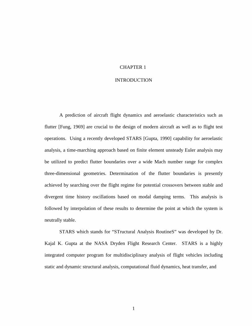
15

following equation results which gives the perturbed pressure ratio across the shock as a

function of Mach number and impact angle.

1

2

)(2

11−

∞∞

−′−+=

′ γγ

θθγoo

o SinMPP

PP

(3-3)

Since the unsteady wave equation is applied as a small perturbation to the mean flow at

10°, the three-dimensional relaxing effects associated with conical flow are taken into

account. This improves the prediction of the surface pressure considerably as compared

with results shown in Figure 2.2 and Figure 2.3. Figure 3.2 and Figure 3.3 illustrate the

improved results. Be sure to note that the percent error for the unperturbed case

discussed in the previous chapter averages about 65 percent whereas the percent error for

the P.S. averages approximately 5 percent. The perturbation solution (P.S.) clearly

improves the prediction of the surface pressure for conical flow.

The Modified Newtonian method, Tangent-Cone method, as well as the piston

method were all analyzed as a small perturbation to a given mean flow over a wide range

of Mach numbers and geometries. Hence, it is clearly shown in Appendix A on page 60

in numerous graphs that the piston theory is the most feasible modeling technique for

implementation into STARS due to its generality and accuracy over these ranges.

16

Cone Cp Versus Mach # Perturbed From 10° to:

0.06

0.1

0.14

0.18

0.22

1 2 3 4 5 6 7 8Mach #

ExactPerturbed

Cp

Mean Flow->10°

12.5°

Figure 3.2. Cp Of A Cone Perturbed About The Mean Flow Of 10° To 12.5°

% Error Versus Mach # Perturbed From 10° to:

0

1

2

3

4

5

6

7

8

1 2 3 4 5 6 7 8Mach #

% E

rror

12.5°

Figure 3.3. % Error Vs. Mach Number For Cp Of A Cone Perturbed From 10° To 12.5°

17

Derivation and Rationale of the Piston Perturbation Method

Since the piston method is the chosen supersonic modeling technique to be used

as a perturbation to the steady finite element Euler solution for aeroelastic analysis, a full

understanding of this method is necessary. This will be done by first discussing the

derivation of the unsteady wave equation. Next, the valid assumptions of this method by

Lighthill [1952] and Ashley [1956] are discussed. And finally, rational for the unsteady

wave equation to be used as a small perturbation to the mean flow to improve the

prediction of the pressure along a given surface is discussed.

As previously noted by Ashley [1956] in chapter 2, it is assumed that if a piston

generates only simple waves and produces no entropy changes, the exact expression for

the instantaneous pressure p(t) on its face is depicted by the simple unsteady wave

equation. A brief derivation of this equation taken from Anderson [190] is as follows:

To develop the governing equations for a finite wave, the continuity equation in

the following form is first considered:

( ) 0=•∇+ VDtD rr

ρρ (3-4)

Also, from thermodynamics, ρ = ρ (p, s). Therefore,

ds

sdp

pd

ps

+

=

δδρ

δδρρ

(3-5)

18

And since ds = 0 for isentropic flow Equation (3-5) becomes,

DtDp

aDtD

2

1=ρ (3-6)

By substitution of Eq. (3-6) into Eq. (3-4), the following equation is generated:

( ) 012 =•∇+ V

DtDp

arr

ρ (3-7)

The previous equation written for one-dimensional flow becomes,

01

2 =+

+

xu

xpu

tp

a δδρ

δδ

δδ

(3-8)

The momentum equation without body forces is now considered:

p

DtVD ∇−=

rr

ρ (3-9)

And for one-dimensional flow,

19

01 =++xp

xuu

tu

δδ

ρδδ

δδ (3-10)

Anderson goes on to apply the method of characteristics and Riemann invariants along

with the following equation for a calorically perfect gas:

ργpa =2 (3-11)

Also, recalling that the process is isentropic, the following equation also applies:

)1/(22

)1/(1

−− == γγγγ acTcp (3-12)

Finally, the next equation relates a and u at any local point in a simple expansion wave:

−−=∞∞ a

uaa

211 γ

(3-13)

Recalling that RTa γ= and implementing into the previous equation gives the

following,

−−=∞∞ a

uTT

211 γ

(3-14)

20

And because the flow is isentropic, )1/()/()/(/ −∞∞∞ == γγγρρ TTpp . Hence, the

previous equation yields the pressure and density ratio in a simple expansion wave as a

function of the local gas velocity in the wave,

)1/(2

211

−

∞∞

−−=γ

γρρ

au

(3-15)

)1/(2

211

−

∞∞

−−=γγ

γau

pp

(3-16)

Based on the previous assumptions by Ashley that if a piston generates only simple waves

and produces no entropy changes, the exact expression for the instantaneous pressure p(t)

on its face is depicted by the simple unsteady wave shown here as Equation (3-16).

Lighthill [1952] states that the unsteady wave equation is expected to be

reasonably accurate if the pressure on the surface remains within the range 0.2 to 3.5

times the mainstream pressure. These values are obtained with the conditions that

motions have large Mach number and [ ] 1)/()/( <×+ UccM ωεδ . Lighthill assumes that

Mδis bounded by less than 1 where δ is the maximum inclination of the airfoil surface to

the stream or impact angle. These limitations are based on the assumption that |u| in the

unsteady wave equation never exceeds the speed of sound in the undisturbed fluid. In an

oscillation with maximum displacement, ε and frequency ω/2π, the condition for u is

written by Lighthill as

21

∞<+ aUδεω (3-17)

By dividing Eq. (3-17) by, a∞

[ ] 1)/()/( <×+ UccM ωεδ (3-18)

where M = U/a∞ and c is the chord of an airfoil such that ωc/U is the frequency

parameter. Finally, Lighthill discusses that the unsteady wave equation may be improved

by use of the “shock expansion” theory, which takes into account the exact pressure

change at the shock and assumes a simple wave behind the shock. This concept is very

similar to the proposed “Piston Perturbation” method which is discussed in the next

paragraph.

Since a clear limitation of the unsteady wave equation is the impact angle δ, it

would stand to reason based on Eq. (3-18) with M >>1 that the smaller the impact angle

the better the results. This is precisely the reason why the cone in Figure 3.2 shows much

better results than the same cone at the same angle in Figure 2.2. Recall that in Figure

3.2, a 10° cone is perturbed 2.5° form the mean flow which in this case was determined

by shock expansion theory. By making the impact angle, δ, much smaller and perturbing

about the mean flow, the accuracy of the surface pressure is significantly improved.

An application of the unsteady wave equation as a small perturbation to a given

mean flow in STARS is derived below. Refer to Figure 3.4.

22

Figure 3.4. Simplistic Illustration Of A Locally Applied Perturbation To The Mean Flow

As before, the same equations are revisited. The perturbed pressure, P′, is solved with

respect to P∞ as follows,

o

o

PP

PP

PP ′

=′

∞∞

(3-19)

The unsteady wave equation is applied as a small perturbation to the mean flow which in

this case is also Po/P∞,

1

2

211

−

∞∞

∆−+=′ γ

γ

γo

o

au

PP

PP

(3-20)

However, in this situation, the velocity of the body Vb is non-zero. Hence,

∆u = Vs·n′ + Vb·n′ where Vs is the unperturbed surface velocity, Vb is the velocity of the

body (i.e. panel), n is the unperturbed outward normal unit vector, and n′ is the perturbed

outward normal unit vector. These values as well as Po, ao, and P∞ are readily available

23

via STARS steady finite element Euler solution. Implementation of ∆u in Eq. (3-20),

yields the following,

1

2

211

−

∞∞

′⋅+′⋅−+=′ γ

γ

γo

bso

anVnV

PP

PP

(3-21)

STARS Implementation

The “perturbation solution” technique is implemented in STARS for the

enhancement of aeroelastic analysis in the following manner: Initially, a supersonic

steady-state solution for a three-dimensional flow field is obtained with the use of the

finite element Euler methodology. The flow variables, which take into account the three-

dimensional effects and non-linearities such as shock interactions, are saved and used as a

mean flow to the starting point of the aeroelastic simulation. Once these variables are

obtained, they may be saved and used for future simulations given the structure is not

significantly altered. With the steady Euler solution given as the mean flow, modal

superposition is applied in the simulated aerodynamic structure to represent the

aeroelastic effects. The modes of vibration are perturbed which represents a perturbation

to the mean flow. Next, an application of the isentropic wave equation previously

discussed is locally applied as a perturbation to the mean flow at every point. The

pressure ratios obtained by the P.S. are then used in the coupled structural dynamic

24

solutions which are numerically integrated to find a generalized displacement “q” shown

as:

[ ] [ ] [ ]PqKqM =⋅+⋅ && (3-22)

Here [M] and [K] are the mass matrix, and the stiffness matrix respectively, obtained in

STARS by a finite element structural analysis routine given the structural properties of

the system. [P] is the force matrix obtained by the piston perturbation method. Once the

generalized displacement for every point on the aeroelastic surface is determined, the

values are multiplied by the mode shapes to determine the actual displacement for

calculation of a new set of transient data.

Given the new structural deflections based on the previous aerodynamic pressures,

a new outward normal velocity is given for the next calculation of the pressures. This

process repeats until enough transient data is acquired to determine the stability

characteristics of the perturbed aerodynamic system. Finally, the flutter boundaries are

then verified and refined with the non-linear time marching Euler method.

25

CHAPTER 4

RESULTS

It will be shown that the Piston Perturbation method accurately predicts surface

pressure for a number of different geometrical configurations in the supersonic flow

regime. It will also be shown that the estimated flutter boundaries of a Generic

Hypersonic Vehicle (GHV) obtained by this method are sufficiently close to the flutter

boundaries obtained by the Euler method. Hence, the estimated CFD solution may then

be used for refinement which requires significantly fewer transient calculations. This

GHV is also used to compare predicted flutter boundaries, and run time between the

perturbation solution and the Euler solution.

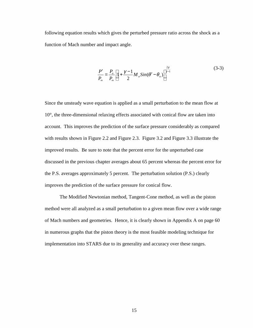
Simple Perturbed Wedge

A simple perturbed wedge exemplifies the validly of this method over a range of

Mach numbers for perturbations about the mean flow in compression and expansion

shown in Figure 4.1 and Figure 4.2. respectively.

26

Wedge Cp Versus Mach # Perturbed From 5° to:

0

0.1

0.2

0.3

0.4

1 2 3 4 5 6 7 8Mach #

ExactPerturbed

Cp

Mean Flow->5°

10°7.5°

12.5°

Figure 4.1. A Simple Perturbed Wedge In Compression

Wedge Cp Versus Mach # Perturbed From 12.5°

0.00

0.20

0.40

0.60

1 2 3 4 5 6 7 8Mach #

ExactPerturbed

10°

Cp

5°7.5°

<-Mean Flow12.5°

Figure 4.2. A Simple Perturbed Wedge In Expansion

The errors for this process are minimal when the assumptions and limitations previously

discussed by Ashley and Lighthill are applied. These assumptions again are that the

27

pressure ratios does not exceed the range of 0.2 to 3.5. with δ small and M >> 1, these

assumptions are met. Since the majority of flutter analysis deals mostly with small

perturbations this criteria holds for a wide range of Mach numbers and geometries.

To better explain the benefits and limitations of this method, a series of charts

similar to Figure 4.1, and Figure 4.2 are generated. The left column of the figure is

similar to the above figure and the column on the right will show the representative

percent error as compared with an NACA Technical Note titled “Tables and charts of

Flow Parameters Across Oblique Shocks” by Neice [1948]. The first set of charts shown

below in Figure 4.3 illustrate a more complete set of data for a simple wedge in

compression. Notice how the percent error increases as the angle from which the solution

is perturbed decreases. This shows that a small perturbation about a strong mean flow

condition gives more accurate results. Also note how the percent error increases

proportional to the perturbation angle. This phenomena shows that by increasing δ, the

piston velocity starts to approach the local speed of sound which is an obvious limitation.

Next, a similar series of charts show a more complete data set for a simple wedge in

expansion.


0

0.2

0.4

0.6

0.8

1

1 2 3 4 5 6 7 8Mach #

ExactPerturbed

Cp

Mean Flow->20°

22.5°


0

5

10

15

20

25

30

1 2 3 4 5 6 7 8Mach #

% E

rror

22.5°

28


0.1

0.3

0.5

0.7

0.9

1 2 3 4 5 6 7 8Mach #

ExactPerturbed

Cp

Mean Flow->15° 17.5°

20°

22.5°


0

5

10

15

20

25

30

1 2 3 4 5 6 7 8Mach #

% E

rror

20°

17.5°

22.5°

Cone Cp Versus Mach # Perturbed From 12.5° to:

0.1

0.2

0.3

0.4

0.5

0.6

0.7

0.8

1 2 3 4 5 6 7 8Mach #

ExactPerturbed

Cp

Mean Flow->12.5°

20°

15°

17.5°

% Error Versus Mach # Perturbed From 12.5° to:

0

5

10

15

20

25

1 2 3 4 5 6 7 8Mach #%

Err

or

20°

15°

17.5°


0

0.1

0.2

0.3

0.4

0.5

0.6

0.7

0.8

1 2 3 4 5 6 7 8Mach #

ExactPerturbed

Cp

Mean Flow->10°

12.5°

15°

17.5°


0

5

10

15

20

25

30

1 2 3 4 5 6 7 8Mach #

% E

rror

12.5°

15°

17.5°

Wedge Cp Versus Mach # Perturbed From 7.5° to:

0

0.1

0.2

0.3

0.4

1 2 3 4 5 6 7 8Mach #

ExactPerturbed

Cp

Mean Flow->7.5° 10°

12.5°

15°


0

5

10

15

20

25

30

1 2 3 4 5 6 7 8Mach #

% E

rror

12.5°

10°

15°

29


0

0.1

0.2

0.3

0.4

1 2 3 4 5 6 7 8Mach #

ExactPerturbed

Cp

Mean Flow->5°

10°

7.5°

12.5°


0

5

10

15

20

25

30

1 2 3 4 5 6 7 8Mach #

% E

rror

12.5°

10°

7.5°

Figure 4.3. More Complete Data Set For A Simple Wedge In Compression


0.1

0.2

0.3

0.4

0.5

0.6

0.7

0.8

0.9

1 2 3 4 5 6 7 8Mach #

ExactPerturbed

Cp

<-Mean Flow22.5°

17.5°

12.5°

15°


0

5

10

15

20

25

30

1 2 3 4 5 6 7 8Mach #

% E

rror

12.5°15°

17.5°


0

0.1

0.2

0.3

0.4

0.5

0.6

1 2 3 4 5 6 7 8Mach #

ExactPerturbed

Cp

<-Mean Flow15°

12.5°

7.5°10°


0

5

10

15

20

25

30

1 2 3 4 5 6 7 8Mach #

% E

rror

12.5°

10°

7.5°

30

Wedge Cp Versus Mach # Perturbed From 12.5°

0.00

0.10

0.20

0.30

0.40

0.50

0.60

1 2 3 4 5 6 7 8Mach #

ExactPerturbed

10°

Cp

5°7.5°

<-Mean Flow12.5°


0

5

10

15

20

25

30

1 2 3 4 5 6 7 8Mach #

10°

5°

7.5°

% E

rror


0

0.1

0.2

0.3

0.4

1 2 3 4 5 6 7 8Mach #

ExactPerturbed

Cp

<-Mean Flow10°

7.5°5°


0

5

10

15

20

25

30

1 2 3 4 5 6 7 8Mach #%

Err

or

5°

7.5°


0

0.1

0.2

0.3

1 2 3 4 5 6 7 8Mach #

ExactPerturbed

Cp

<-Mean Flow7.5°

5°


0

5

10

15

20

25

30

1 2 3 4 5 6 7 8Mach #

% E

rror

5°

Figure 4.4. A More Complete Data Set For A Simple Wedge In Expansion

31

Simple Perturbed Cone

The P.S. also predicts pressure about more three dimensional surfaces, such as

cones, over a range of Mach numbers in compression as well as expansion. This is

shown in Figure 4.5 and Figure 4.6. Again, the P.S gives accurate results of surface

pressure since it is applied as a small perturbation to the mean flow where the three-

dimensional relaxation effects are accounted for.


0

0.1

0.2

0.3

0.4

1 2 3 4 5 6 7 8Mach #

ExactPerturbed

Cp

Mean Flow->10°

12.5°

15°

17.5°

Figure 4.5. A Simple Perturbed Cone In Compression

32


0.00

0.05

0.10

0.15

0.20

1 2 3 4 5 6 7 8Mach #

ExactPerturbed

10°Cp

5°7.5°

<-Mean Flow12.5°

Figure 4.6. A Simple Perturbed Cone In Expansion

Notice the perturbed curve from 12.5° to 5° shown in Figure 4.6 above. This is the result

of a perturbation condition greater than the mean flow condition. Hence, an obvious

limitation of this method. Additional illustrations of cone perturbation similar to the

previous two figures are shown below. Since these charts show perturbations of cones

with various angles, this phenomenon will be shown again in expansion.


0.2

0.3

0.4

0.5

1 2 3 4 5 6 7 8Mach #

ExactPerturbed

Cp

Mean Flow->20°

22.5°


0

5

10

15

20

25

30

1 2 3 4 5 6 7 8Mach #

% E

rror

22.5°

33


0.1

0.2

0.3

0.4

0.5

1 2 3 4 5 6 7 8Mach #

ExactPerturbed

Cp

Mean Flow->15°

20°

22.5°

17.5°


0

5

10

15

20

25

30

1 2 3 4 5 6 7 8Mach #

% E

rror

20°

22.5°

17.5°


0.05

0.15

0.25

0.35

0.45

1 2 3 4 5 6 7 8Mach #

ExactPerturbed

Cp

Mean Flow->12.5°

20°

15°

17.5°


0

5

10

15

20

25

30

1 2 3 4 5 6 7 8Mach #%

Err

or

20°

15°

17.5°


0

0.1

0.2

0.3

0.4

1 2 3 4 5 6 7 8Mach #

ExactPerturbed

Cp

Mean Flow->10°

12.5°

15°

17.5°


0

5

10

15

20

25

30

1 2 3 4 5 6 7 8Mach #

% E

rror

12.5°

15°

17.5°


0

0.05

0.1

0.15

0.2

0.25

0.3

1.00 2.00 3.00 4.00 5.00 6.00 7.00 8.00Mach #

ExactPerturbed

Cp

Mean Flow->7.5°

12.5°

10°

15°


0

5

10

15

20

25

30

1 2 3 4 5 6 7 8Mach #

% E

rror

12.5°

10°

15°

34


0

0.1

0.2

1.00 2.00 3.00 4.00 5.00 6.00 7.00 8.00Mach #

ExactPerturbed

Cp

Mean Flow->5°

10°

7.5°

12.5°


0

10

20

30

40

1 2 3 4 5 6 7 8Mach #

% E

rror

12.5°

10°

7.5°

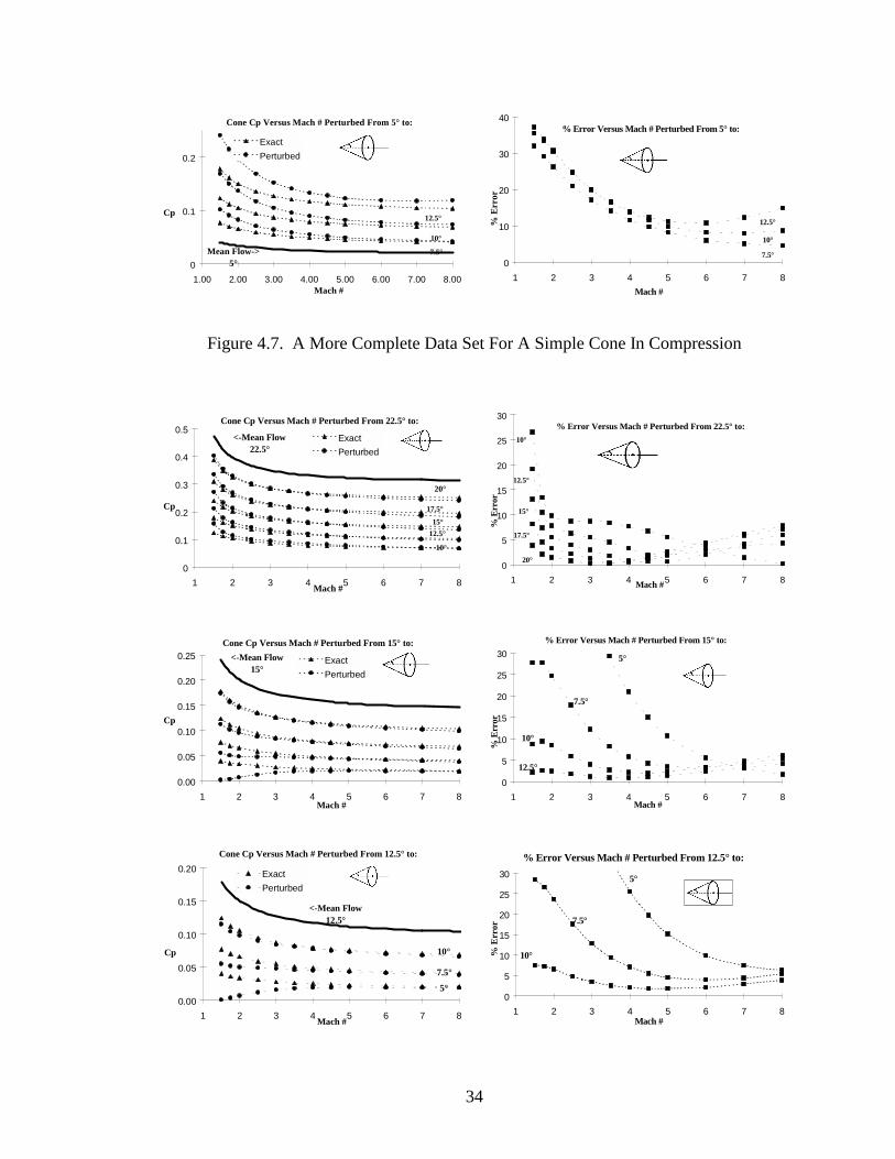
Figure 4.7. A More Complete Data Set For A Simple Cone In Compression


0

0.1

0.2

0.3

0.4

0.5

1 2 3 4 5 6 7 8Mach #

ExactPerturbed

20°

Cp15°

17.5°

<-Mean Flow22.5°

10°

12.5°


0

5

10

15

20

25

30

1 2 3 4 5 6 7 8Mach #

10°

% E

rror

20°

17.5°

15°

12.5°


0.00

0.05

0.10

0.15

0.20

0.25

1 2 3 4 5 6 7 8Mach #

ExactPerturbed

Cp

<-Mean Flow15°


0

5

10

15

20

25

30

1 2 3 4 5 6 7 8Mach #

10°

5°

7.5°

% E

rror

12.5°


0.00

0.05

0.10

0.15

0.20

1 2 3 4 5 6 7 8Mach #

ExactPerturbed

10°Cp

5°

7.5°

<-Mean Flow12.5°


0

5

10

15

20

25

30

1 2 3 4 5 6 7 8Mach #

10°

5°

7.5°

% E

rror

35


-0.04

-0.02

0

0.02

0.04

0.06

0.08

1 2 3 4 5 6 7 8Mach #

PerturbedExact

Cp

<-Mean Flow7.5°

5°

2.5°


0

50

100

150

200

250

1 2 3 4 5 6 7 8Mach #

% E

rror

2.5°

5°


-0.02

-0.01

0

0.01

0.02

0.03

0.04

1 2 3 4 5 6 7 8Mach #

ExactPerturbed

Cp

<-Mean Flow5°

2.5°


0

50

100

150

200

250

1 2 3 4 5 6 7 8Mach #

% E

rror 2.5°

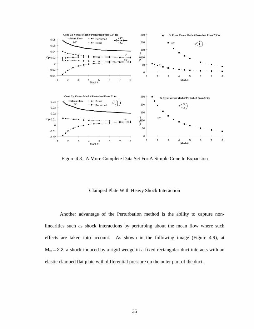
Figure 4.8. A More Complete Data Set For A Simple Cone In Expansion

Clamped Plate With Heavy Shock Interaction

Another advantage of the Perturbation method is the ability to capture non-

linearities such as shock interactions by perturbing about the mean flow where such

effects are taken into account. As shown in the following image (Figure 4.9), at

M∞ = 2.2, a shock induced by a rigid wedge in a fixed rectangular duct interacts with an

elastic clamped flat plate with differential pressure on the outer part of the duct.

36

Figure 4.9. A Fixed Rectangular Duct With An Elastically Flexible Clamped Flat Plate

A side view of this geometry (Figure 4.10) shows the pressure contours generated by

steady Euler analysis. Notice the shock interactions due to the wedge and rigid

boundaries of the geometry.

Figure 4.10. A Side View Showing The Pressure Contours Of The Heavy Shock Interactions With The Elastic Plate

37

A magnified view for the steady state deformation of the elastic plate generated by the

unsteady Euler equations is shown in Figure 4.11(a). This deformation is generated by

first running a steady Euler analysis to obtain convergence of the aerodynamic properties

throughout the duct. Next, the process is restarted, this time allowing the plate to

oscillate due to the resulting aerodynamic forces just acquired from the steady Euler

analysis. After the plate’s oscillation damps, steady state deflection is achieved. Notice

the plate’s outward deformation due to the shock induced by the rigid wedge.

As a comparison, unsteady aerodynamic analysis via piston theory (as opposed to

unsteady Euler analysis) is performed and shown below in Figure 4.11(b). Since the

piston theory takes into account only the local conditions, pressure induced by the shock

is unaccounted for which causes large errors in the steady state deformation.

The Perturbation solution is now applied with the following results in Figure

4.11(c). Since the perturbation method perturbs about the mean flow, the non-linearities

induced by the shock are accounted for giving more accurate results as compared with the

unsteady Euler analysis shown in Figure 4.11(a).

38

Figure 4.11. Steady State Deformation Of The Elastic Plate Generated By: (A) Unsteady Euler Analysis, (B) Piston Theory, (C) Perturbation Method

Steady Perturbation Analysis

As another example of the accuracy and generality of the Perturbation method,

pressures at three sectional cuts on a Generic Hypersonic Vehicle (GHV) are calculated at

Mach 2.2 with a 5º angle of attack. The Perturbation method results are calculated by

applying an application of the unsteady wave equation as a 1° perturbation about the

mean flow (calculated by steady Euler analysis) at 4°,. The pressure via Piston theory,

and Euler analysis at 5° angle of attack is also calculated for comparison and shown in

Figure 4.12.

39

-0.1

0

0.1

0.2

0.3

0 0.1 0.2 0.3 0.4 0.5 0.6 0.7 0.8 0.9 1x/xr

Cp

EulerP.S.Piston

Section Cut 1

-0.2

-0.1

0

0.1

0.2

0.3

0.7 0.75 0.8 0.85 0.9 0.95 1x/xr

Cp

EulerP.S.Piston

Section Cut 2

-0.3

-0.2

-0.1

0

0.1

0.2

0.3

0.85 0.9 0.95 1x/xr

Cp

EulerP.S.piston

Section Cut 3

Figure 4.12. Pressure Comparisons At 5º Angle Of Attack Using Euler, Piston, And

Perturbation Method At Three Sectional Cuts On A GHV

40

GHV Flutter Analysis

As a another illustration, a surface mesh of the baseline configuration for the

GHV is generated (Figure 4.13) and flutter analysis is performed in the following manner:

Figure 4.13. GHV Baseline Surface Mesh

Given the GHV’s surface mesh, a finite-element structural model is developed to obtain

the structural mode shapes and frequencies (details referenced under Gupta, 1990, 1991,

1992). Next, a steady solution to the flow field at Mach 2.2 and 0° angle of attack is

obtained by the finite-element Euler methodology. This solution is then used as the mean

flow condition about which the perturbation solution is applied. For the aeroelastic

simulation, a 9 mode solution is run for 705 time steps which is approximately 7 cycles of

mode 1. Using the unsteady Euler analysis, transient data of 4 dynamic pressures is

analyzed and the flutter boundary is estimated through polynomial interpolation. For the

41

purpose of run-time comparison, the same procedure is used for the perturbation solution.

In this case of course, the piston perturbation method is applied in place of the unsteady

Euler analysis.

As seen in Figure 4.14, the difference among flutter boundary estimates between

the two codes for this case is found to be less than 4%, however the difference in run

times between the two codes is extremely significant.

-0.4

-0.2

0

0.2

0.05 0.1 0.15 0.2 0.25 0.3 0.35density

mod

al d

ampi

ng r

atio

EulerP.S.

Boundary

1 Transient

1 10 100 1000 10000 100000

CPU Time (Minutes)

Boundary

1 Transient

Euler Perturbation Solution

Figure 4.14. Flutter Boundary And Run-Time Comparisons At M=2.2 With 705 Time Steps / Transient

42

Run time for the perturbation solution (P.S.) estimate is 3 minutes for each transient or

approximately 15 minutes to identify the flutter boundary. On the other hand, run time

for the Euler solution used to define the flutter boundary is 117 hours for each transient

and approximately 469 hours to identify the boundary. All simulations are run on an IBM

RS6000 3BT workstation.

Cone & Swept Wing Configuration

As a final illustration of the perturbation method, a geometry consisting of a

combination “Cone and Swept Wing Configuration” (CSWC) is considered to examine

the flow characteristics about a more three dimensional flow field. The analysis will be

done in the same manner as the GHV, with a wider test range. The following geometry

(Figure 4.15) shows the baseline surface mesh used by the flow solver in the aerodynamic

analysis. The symmetrically cambered wing is swept 42 degrees which makes the design

Mach number when placed on the 15° cone approximately 1.6. Since steep gradients

require a fine mesh and more computation time, the cone is tapered aft of the swept wing.

Since the taper is gradual and the flow is supersonic (flow effects may not propagate

forward), this area may be coarsely meshed aiding in computational efficiency. Figure

4.16 shows the specific dimensions of the CSWC geometry as well as detailed

information used to create the aerodynamic mesh so the CSWC may be regenerated at

another time.

43

Figure 4.15. Cone & Swept Wing Configuration Baseline Mesh

Figure 4.16. CSWC Specific Dimensions

44

The values for Figure 4.16 are tabulated below in Table 4.1. Also, the data file

containing further information used to generate the mesh of the aerodynamic flow solver

is located in Appendix B on page 80.

Table 4.1. Point Location for The CSWC

Point Location# x y z0 0.0000 0.0000 0.00001 1.7159 0.4598 0.00002 5.6818 1.5226 0.00003 3.8975 2.4242 0.00004 5.9394 2.4242 0.00005 6.6024 4.8597 0.00006 7.5017 4.8597 0.00007 15.0000 0.0000 0.00008 -5.0000 0.0000 0.00009 15.0000 0.0000 0.0000

The symmetrical swept wing configuration is generated using the following equation:

( )xccxz lu −±= ε4, (4-1)

ε is chosen to be 0.05 which will cause the mean flow to see an impact angle of

approximately 5°. A cross-section of this wing is shown below in Figure 4.17.

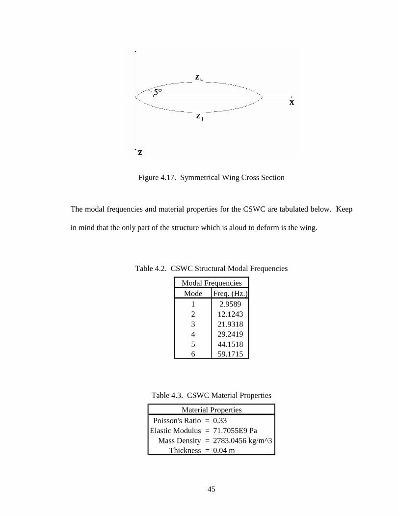
45

Figure 4.17. Symmetrical Wing Cross Section

The modal frequencies and material properties for the CSWC are tabulated below. Keep

in mind that the only part of the structure which is aloud to deform is the wing.

Table 4.2. CSWC Structural Modal Frequencies

Modal FrequenciesMode Freq. (Hz.)

1 2.95892 12.12433 21.93184 29.24195 44.15186 59.1715

Table 4.3. CSWC Material Properties

Material PropertiesPoisson's Ratio = 0.33

Elastic Modulus = 71.7055E9 PaMass Density = 2783.0456 kg/m^3

Thickness = 0.04 m

46

Flutter analysis at Mach 1.3 is one Mach number considered along with Mach 1.6,

Mach 2.0, Mach 2.4, and Mach 2.8. Figure 4.18 shows the pressure contours generated

by the steady finite element Euler analysis at Mach 1.3. The pressure contours shown

here are used as the mean flow condition for the unsteady Euler analysis and the P.S.

Figure 4.18. Pressure Contours Generated Using Steady Finite Element Euler Analysis at Mach 1.3

The perturbation method and the Piston method are used to determine the flutter

boundary at Mach 1.3. These boundaries are determined by analyzing the transients of

the different modes. Usually, the most obvious mode to determine the stability of the

system is mode 1. For the perturbation and Piston methods, a half interval search is

conducted to determine the stability of the system. In other words, an unsteady analysis

using piston or P.S. is run at a given density. Say one transient is convergent at a given

density and another is divergent at a different density. The value half way between the

47

two densities is the new value used in another analysis. This analysis is repeated until a

neutral transient in mode 1 is determined. Since a full transient takes only minutes to run,

several transients may be run to pinpoint the flutter point for both methods. Next, these

boundaries are compared with the flutter boundary determined by the unsteady Euler

analysis. Since this analysis requires significantly more computation time, on the order of

days, a logarithmic decrement of mode 1 is used to determine the modal damping ratio

for each transient. Once enough transients are generated (usually 2-4), the damping ratio

vs. Mach number points are fit with a cubic spline curve fit to determine where the curve

crosses the neutral damping axis. This intersection is assumed to be the flutter point

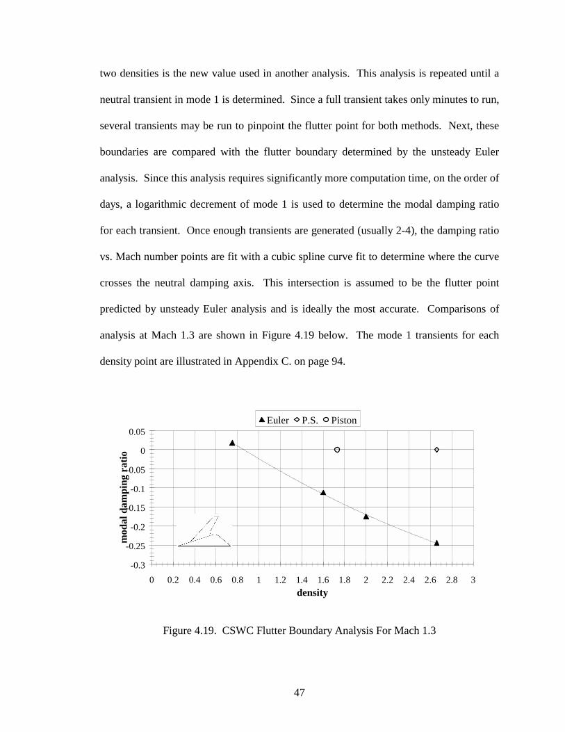
predicted by unsteady Euler analysis and is ideally the most accurate. Comparisons of

analysis at Mach 1.3 are shown in Figure 4.19 below. The mode 1 transients for each

density point are illustrated in Appendix C. on page 94.

-0.3

-0.25

-0.2

-0.15

-0.1

-0.05

0

0.05

0 0.2 0.4 0.6 0.8 1 1.2 1.4 1.6 1.8 2 2.2 2.4 2.6 2.8 3density

mod

al d

ampi

ng r

atio

Euler P.S. Piston

Figure 4.19. CSWC Flutter Boundary Analysis For Mach 1.3

48

In Figure 4.19 above, the Euler analysis predicts a flutter point at about ρ equal to 0.85

kilograms per meter cubed which is not at all close to the estimate given by the P.S. The

piston method however, is considerably closer to the flutter point. This, however, is by

chance since both methods give a very poor estimate at very low Mach. Thus far, this

proves the assumptions previously discussed by Lighthill and Ashley that Mach number

must be much greater than 1 for accurate results. A trend which gives a better

understanding of this phenomenon is developed, graphed, and discussed later.

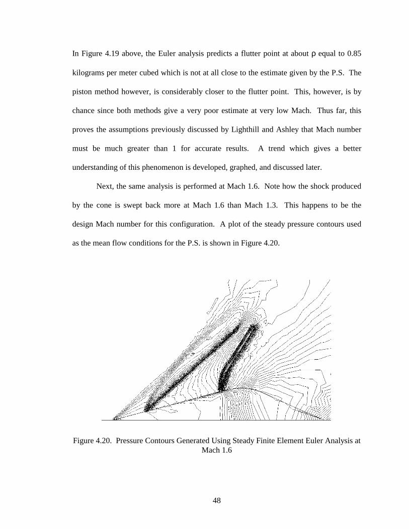
Next, the same analysis is performed at Mach 1.6. Note how the shock produced

by the cone is swept back more at Mach 1.6 than Mach 1.3. This happens to be the

design Mach number for this configuration. A plot of the steady pressure contours used

as the mean flow conditions for the P.S. is shown in Figure 4.20.

Figure 4.20. Pressure Contours Generated Using Steady Finite Element Euler Analysis at Mach 1.6

49

Comparisons of analysis are done in the same manner as with Mach 1.3 above and is

shown here in Figure 4.21.

-0.02

0

0.02

0.04

0.06

0.08

0.1

1.2 1.3 1.4 1.5 1.6 1.7 1.8 1.9 2 2.1 2.2density

mod

al d

ampi

ng r

atio

Euler P.S. Piston

Figure 4.21. CSWC Flutter Boundary Analysis For Mach 1.6

As shown in Figure 4.21, the P.S. very closely predicts the flutter point determined by the

unsteady Euler analysis. This again supports the assumptions made earlier that for this

method to be accurate, the Mach number must be significantly greater than 1.

The same analysis is repeated for Mach 2.0, Mach 2.4, and Mach 2.8 and shown

in Figure 4.22. Notice the shock interactions in the mean flow for these Mach numbers.

This is another example where the Perturbation method is able to capture the non-linear

three-dimensional flow characteristics by accounting for these anomalies in the mean

flow.

50

Figure 4.22. CSWC Pressure Contours Generated Using Steady Finite Element Euler Analysis (left column) and Flutter Boundary Analysis (right column)

The flutter boundary over the whole Mach range is shown below in tabular form (Table

4.4) and illustrated in Figure 4.23 and Figure 4.24. :

-0.04

-0.03

-0.02

-0.01

0

0.01

0.02

0.03

0.04

0.9 0.95 1 1.05 1.1 1.15 1.2 1.25 1.3 1.35 1.4 1.45density

mod

al d

ampi

ng r

atio

Euler P.S. Piston

(a) Mach 2.0

-0.02

-0.01

0

0.01

0.02

0.03

0.04

0.65 0.7 0.75 0.8 0.85 0.9 0.95 1 1.05density

mod

al d

ampi

ng ra

tio

Euler P.S. Piston

(b) Mach 2.4

-0.08

-0.06

-0.04

-0.02

0

0.02

0.04

0.57 0.59 0.61 0.63 0.65 0.67 0.69 0.71 0.73 0.75 0.77 0.79 0.81

density

mod

al d

ampi

ng r

atio

Euler P.S. Piston

(c) Mach 2.8

51

Table 4.4. CSWC Flutter Boundary Data

Euler Perturbation Solution Piston TheoryM ρρρρ (kg/m^3) ρρρρ (kg/m^3) % Error ρρρρ (kg/m^3) % Error

1.3 0.85 2.66 213 1.73 1041.6 2.015 1.94 4 1.22 392.0 1.29 1.33 3 0.96 262.4 0.92 0.98 7 0.745 192.8 0.72 0.79 10 0.59 18

Flutter Point vs. Mach Number for CSWC

0

1

2

3

1.2 1.4 1.6 1.8 2.0 2.2 2.4 2.6 2.8Mach #

Den

sity

(kg/

m^3

)

EulerPerturbationPiston

Figure 4.23. CSWC Flutter Boundary

Percent Error vs. Mach Number for CSWC

0

10

20

30

40

50

1.4 1.6 1.8 2.0 2.2 2.4 2.6 2.8Mach #

% E

rror

PerturbationPiston

Figure 4.24. CSWC Flutter Boundary % Error Analysis

52

The graphical representations in Appendix A on page 60 show very similar trends to the

data just illustrated. Based on the data in Appendix A, it stands to reason that as the

Mach number increases, the error via the P.S. remains low whereas the error via piston

theory significantly increases.

53

CHAPTER 5

CONCLUSIONS AND RECOMMENDATIONS

Conclusions

Obtained results reveal that the goal to enhance the practicality of time-marching

supersonic flutter analysis has been achieved. This was accomplished by taking

advantage of the efficient aspects of the supersonic modeling technique known as the

piston theory and applying it as a small perturbation to a given mean flow obtained by the

steady finite element Euler analysis in STARS. By replacing the unsteady Euler

equations with this modeling technique, the results of the unsteady aerodynamic analysis

are produced relatively instantaneously with very little error. This was previously shown

in the aeroelastic analysis of the GHV.

Several supersonic modeling techniques were considered to be implemented into

STARS but the piston theory applied as a perturbation to the mean flow proves to be the

most feasible. The feasibility of this method is a result of the simplicity and easy

implementation into an existing aeroelastic analysis computer program. Since all the

unsteady wave equation needs to be applied as a perturbation to an existing steady mean

54

flow is the local conditions and the perturbed outward normal unit vector, easy and

accurate implementation into an existing computer code with these conditions may be

achieved. Furthermore, by complying with the assumptions and limitations of this

method, and taking advantage of the small perturbations associated with aeroelastic

analysis, the P.S. has proven extremely accurate over a considerably large Mach range.

In addition to the Perturbation Solution’s ability to handle a number of

geometrical configurations over a wide Mach range, it is also very accurate in areas where

non-linearities such as shock interactions occur. In fact, since these areas of shock

interaction are associated with strong mean flow characteristics, this method really

“shines” since the assumptions for validity are high Mach number and small perturbation

from the mean flow. The rigid duct with an elastic plate previously discussed shows

these results.

An added advantage of the presented approach is that the same grid may be used

for the steady CFD solution, the perturbation model, and the time marching CFD

solution. This is significant due to the fact that it takes on the order of hours and in many

cases days to obtain a mean flow solution for a given geometry.

55

Recommendations

Since the aeroelastic analysis performed on the CSWC seems to follow a very

similar trend with that of the steady perturbation analysis shown in Appendix A on page

60, it is highly recommend that validation at Mach numbers greater than Mach 2.8 be

accomplished. Since the steady perturbation analysis shows very small error up to around

Mach 8, it is assumed that the P.S. method with respect to the aeroelastic analysis will be

very accurate as well.

A method initially presented as the “tag method” was briefly discussed but not

looked into much further do to its probable inability to recognize areas of heavy shock

interaction in its analysis. This method also takes advantage of the already existing mean

flow generated by Euler analysis, not as a mean flow for a small perturbation, but as

comparison at every nodal point in the computational domain with several supersonic and

hypersonic modeling techniques. This is done by calculating the pressure for these

modeling techniques and comparing with the pressure of the nodal location. The

modeling technique which predicts the pressure the closest to that point “wins”, is tagged

to that point, and used for further analysis. Since many supersonic configurations are

designed to avoid such anomalies as significant shock interactions, it is recommended

that the “tag method” be given further consideration and compared with the P.S. method.

Also, an improvement in the method in which the damping ratio for the finite

element unsteady Euler analysis performed is needed. At the moment, a logarithmic

decrement is performed and on mode 1 which under certain circumstances is very

difficult.

56

Lastly, since the assumptions and limitations of the Piston Perturbation method

are known, (i.e. 0.2 < pressure ratio 3.5), an accuracy check based on these limitations is

recommended. This analysis would need to determine the amount the pressure has been

perturbed from the mean flow. Then, based on the previous assumptions, a rough error

analysis may be performed on the perturbations which exceed these restrictions. This

should not be too difficult a task and should aid in the efficient and accurate

determination of a given flutter point.

57

BIBLIOGRAPHY

Allen, David H. and Walter E Haisler, Introduction To Aerospace Structural Analysis, Wiley, New York, 1985.

Anderson, John D., Jr., Modern Compressible Flow With Historical Perspective,

McGraw-Hill, New York, 1982. Ashley, Holt, and Garabed Zartarian, “Piston Theory-A New Aerodynamic Tool for the

Aeroelastician,” Presented at the Twenty-Forth Annual Aeroelasticity Meeting, New York, January, 1956.

Bertin, John J. and Michael L. Smith, Aerodynamics For Engineers, 2nd Edition, Prentice-

Hall, New Jersey, 1989. Bonner, E.; Cleaver, W.; and Dunn, K., “Aerodynamic Preliminary Analysis System II.

Part I Theory”, NASA CR-165627, 1981. Cruz, Christopher I. and Gregory J. Sova, “Improved Tangent-Cone Method for the

Aerodynamic Preliminary Analysis System (APAS) Version of the Hypersonic Arbitrary-Body Program”, NASA TM 4165, February, 1990.

Dowel, E.H., et al, A Modern Course in Aeroelasticity, 3rd Edition, Klewer Academic

Publishers, 1995. Fung, Y. C., An Introduction to the Theory of Aeroelasticity, 1st Edition, Dover, New

York, 1969. Gupta, K.K., “STARS - An Integrated General-Purpose Finite Element Structural,

Aeroelastic, and Aeroservoelastic Analysis Computer Program,” NASA TM-101709, June, 1990.

Gupta, K.K., Peterson, K., and Lawson, C., “Multidisciplinary Modeling and Simulation

of a Generic Hypersonic Vehicle,” AIAA-91-5015, AIAA 3rd International Aerospace Planes Conference, Orlando, FL, December, 1991.

58

Gupta, K.K., Peterson, K., and Lawson, C., “On Some Recent Advances in Multidisciplinary Analysis of Hypersonic Vehicles,” AIAA-92-5026, AIAA Fourth International Aerospace Planes Conference, Orlando, FL, December, 1991.

Inman, Daniel J., Engineering Vibration, Prentice-Hall, New Jersey, 1994. John, James E. A., Gas Dynamics, 2nd Edition, Allyn and Bacon, Boston, 1984. Lighthill, M. J., “Oscillating Airfoils at High Mach Number”, Journal of the Aeronautical

Sciences, vol. 20, No. 6, pp. 402-406, June, 1953. Morgan, Homer G., Harry L. Runyan, and Vera Huckel, “Theoretical Considerations of

Flutter at High Mach Numbers,” Presented at the Aeroelasticity-II Session, Twenty-Sixth Annual Meeting, New York, January, 1958.

Marsden, Jerrold E. and Anthony J. Tromba, Vector Calculus, 4th Edition, Freeman, New

York, 1996. Moran, Michael J. and Howard N. Shapiro, Fundamentals Of Engineering

Thermodynamics, 2nd Edition, Wiley, New York, 1992. Neice, Mary M., “Tables and Charts of Flow Parameters Across Oblique Shocks”, NACA

TN 1673, August, 1948. Pittman, Jimmy L. (appendix by C. L. W. Edwards): “Application of Supersonic Linear

Theory and Hypersonic Impact Methods to Three Nonslender Hypersonic airplane Concepts at Mach Numbers From 1.10 to 2.86”, NASA TP-1539, 1979.

Sims, Joseph L., “Tables for Supersonic Flow Around Right Circular Cones at Zero

Angle of Attack”, NASA SP-3004, 1964. Truitt, Robert W., Hypersonic Aerodynamics, Ronald Press Co., 1959.

59

APPENDICES

60

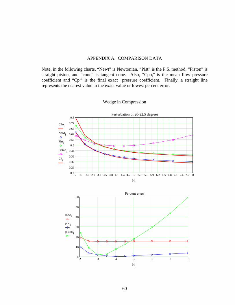
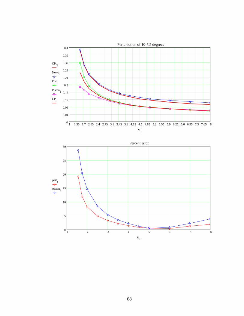
APPENDIX A: COMPARISON DATA Note, in the following charts, “Newt” is Newtonian, “Pist” is the P.S. method, “Piston” is straight piston, and “cone” is tangent cone. Also, “Cpoi” is the mean flow pressure coefficient and “Cpi” is the final exact pressure coefficient. Finally, a straight line represents the nearest value to the exact value or lowest percent error.

Wedge in Compression

2 2.3 2.6 2.9 3.2 3.5 3.8 4.1 4.4 4.7 5 5.3 5.6 5.9 6.2 6.5 6.8 7.1 7.4 7.7 80.2

0.26

0.32

0.38

0.44

0.5

0.56

0.62

0.68

0.74

0.8Perturbation of 20-22.5 degrees

CPoi

Newti

Pisti

Piston i

CPi

Mi

2 3 4 5 6 7 80

10

20

30

40

50

60Percent error

newti

pist i

piston i

Mi

61

1 1.35 1.7 2.05 2.4 2.75 3.1 3.45 3.8 4.15 4.5 4.85 5.2 5.55 5.9 6.25 6.6 6.95 7.3 7.65 80.1

0.17

0.24

0.31

0.38

0.45

0.52

0.59

0.66

0.73


CPoi

Newti

Pisti

Piston i

CPi

Mi

1 2 3 4 5 6 7 80

6.67

13.33

20

26.67

33.33

40Percent error

newti

pist i

piston i

Mi

62

1 1.35 1.7 2.05 2.4 2.75 3.1 3.45 3.8 4.15 4.5 4.85 5.2 5.55 5.9 6.25 6.6 6.95 7.3 7.65 80.1

0.15

0.2

0.25

0.3

0.35

0.4

0.45

0.5

0.55

0.6Perturbation of 12.5-15 degrees

CPoi

Newti

Pisti

Piston i

CPi

Mi

1 2 3 4 5 6 7 80

5

10

15

20

25

30Percent error

newti

pist i

piston i

Mi

63

1 1.35 1.7 2.05 2.4 2.75 3.1 3.45 3.8 4.15 4.5 4.85 5.2 5.55 5.9 6.25 6.6 6.95 7.3 7.65 80

0.06

0.12

0.18

0.24

0.3

0.36

0.42

0.48

0.54


CPoi

Newti

Pisti

Piston i

CPi

Mi

1 2 3 4 5 6 7 80

6.67

13.33

20

26.67

33.33

40Percent error

newti

pist i

piston i

Mi

64

1 1.35 1.7 2.05 2.4 2.75 3.1 3.45 3.8 4.15 4.5 4.85 5.2 5.55 5.9 6.25 6.6 6.95 7.3 7.65 80

0.03

0.06

0.09

0.12

0.15

0.18

0.21

0.24

0.27


CPoi

Newti

Pisti

Piston i

CPi

Mi

1 2 3 4 5 6 7 80

5

10

15

20

25

30Percent error

pist i

piston i

Mi

65

Wedge in Expansion

Note, in the following charts, “Newt” is Newtonian, “Pist” is the P.S. method, “Piston” is straight piston, and “cone” is tangent cone. Also, “Cpoi” is the mean flow pressure coefficient and “Cpi” is the final exact pressure coefficient. Finally, a straight line represents the nearest value to the exact value or lowest percent error.

2 2.3 2.6 2.9 3.2 3.5 3.8 4.1 4.4 4.7 5 5.3 5.6 5.9 6.2 6.5 6.8 7.1 7.4 7.7 80.3

0.35

0.4

0.45

0.5

0.55

0.6

0.65

0.7

0.75


CPoi

Newti

Pisti

Piston i

CPi

Mi

2 3 4 5 6 7 80

8.33

16.67

25

33.33

41.67

50Percent error

newti

pist i

piston i

Mi

66

1 1.35 1.7 2.05 2.4 2.75 3.1 3.45 3.8 4.15 4.5 4.85 5.2 5.55 5.9 6.25 6.6 6.95 7.3 7.65 80.1

0.15

0.2

0.25

0.3

0.35

0.4

0.45

0.5

0.55


CPoi

Newti

Pisti

Pistoni

CPi

Mi

1 2 3 4 5 6 7 80

8.33

16.67

25

33.33

41.67

50Percent error

newti

pisti

piston i

Mi

67

1 1.35 1.7 2.05 2.4 2.75 3.1 3.45 3.8 4.15 4.5 4.85 5.2 5.55 5.9 6.25 6.6 6.95 7.3 7.65 80

0.06

0.12

0.18

0.24

0.3

0.36

0.42

0.48

0.54


CPoi

Newti

Pisti

Piston i

CPi

Mi

1 2 3 4 5 6 7 80

10

20

30

40

50

60Percent error

newti

pist i

piston i

Mi

68

1 1.35 1.7 2.05 2.4 2.75 3.1 3.45 3.8 4.15 4.5 4.85 5.2 5.55 5.9 6.25 6.6 6.95 7.3 7.65 80

0.04

0.08

0.12

0.16

0.2

0.24

0.28

0.32

0.36


CPoi

Newti

Pisti

Piston i

CPi

Mi

1 2 3 4 5 6 7 80

5

10

15

20

25

30Percent error

pisti

piston i

Mi

69

1 1.35 1.7 2.05 2.4 2.75 3.1 3.45 3.8 4.15 4.5 4.85 5.2 5.55 5.9 6.25 6.6 6.95 7.3 7.65 80

0.03

0.06

0.09

0.12

0.15

0.18

0.21

0.24

0.27


CPoi

Newti

Pisti

Piston i

CPi

Mi

1 2 3 4 5 6 7 80

5

10

15

20

25

30Percent error

pist i

piston i

Mi

70

Cone in Compression


1 1.35 1.7 2.05 2.4 2.75 3.1 3.45 3.8 4.15 4.5 4.85 5.2 5.55 5.9 6.25 6.6 6.95 7.3 7.65 80.25

0.28

0.3

0.33

0.35

0.38

0.4

0.43

0.45

0.48


CPoi

Newti

Pisti

Piston7

Conei

CPi

Mi

1 2 3 4 5 6 7 80

10

20

30

40

50Percent error

newti

pisti

piston 7

cone i

Mi

71

1 1.35 1.7 2.05 2.4 2.75 3.1 3.45 3.8 4.15 4.5 4.85 5.2 5.55 5.9 6.25 6.6 6.95 7.3 7.65 80.1

0.15

0.2

0.25

0.3

0.35

0.4

0.45

0.5

0.55

0.6Perturbation of 15 to 17.5 degrees

CPoi

Newti

Pisti

Piston i

CPi

Mi

1 2 3 4 5 6 7 805.33

10.6716

21.3326.67

3237.3342.67

4853.3358.67

6469.3374.67

80Percent error

newt1

pisti

piston i

Mi

72

1 1.35 1.7 2.05 2.4 2.75 3.1 3.45 3.8 4.15 4.5 4.85 5.2 5.55 5.9 6.25 6.6 6.95 7.3 7.65 80.1

0.12

0.13

0.15

0.16

0.18

0.19

0.21

0.22

0.24

0.25Perturbation of 12.5 to 15 degrees

CPoi

Newti

Pisti

Piston11

CPi

Mi

1 2 3 4 5 6 7 80

6

12

18

24

30

36

42

48

54

60Percent error

newti

pisti

piston 11

Mi

73

1 1.35 1.7 2.05 2.4 2.75 3.1 3.45 3.8 4.15 4.5 4.85 5.2 5.55 5.9 6.25 6.6 6.95 7.3 7.65 80.06

0.074

0.088

0.1

0.12

0.13

0.14

0.16

0.17

0.19


CPoi

Newti

Pisti

Piston11

Conei

CPi

Mi

1 2 3 4 5 6 7 80

5

10

15

20

25

30

35

40

45

50Percent error

newti

pist i

piston 11

cone i

Mi

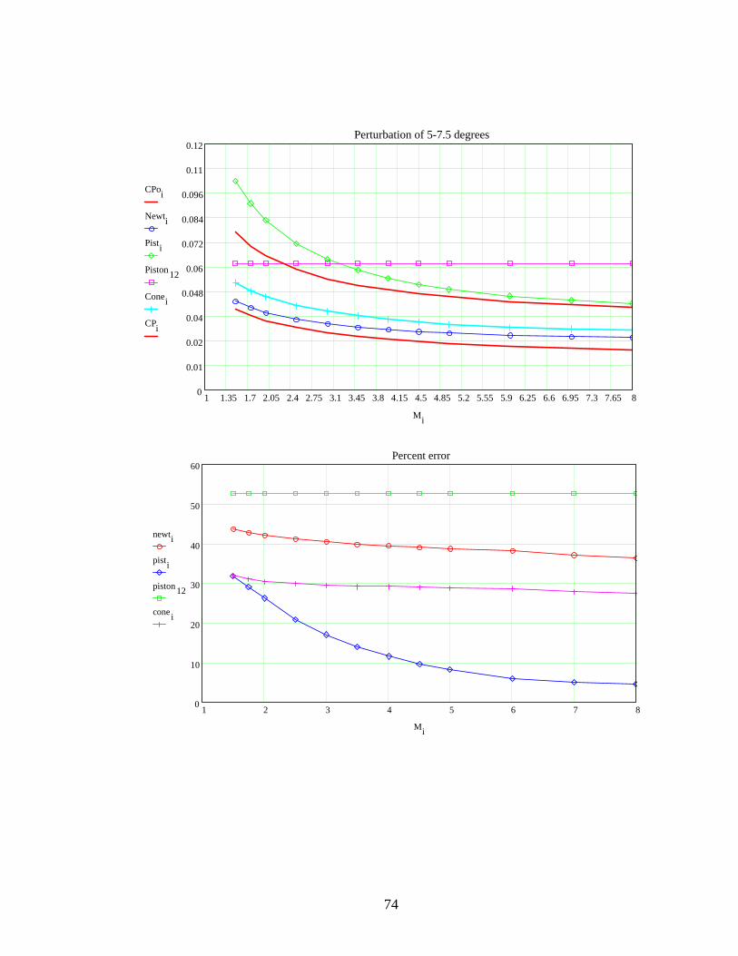
74

1 1.35 1.7 2.05 2.4 2.75 3.1 3.45 3.8 4.15 4.5 4.85 5.2 5.55 5.9 6.25 6.6 6.95 7.3 7.65 80

0.01

0.02

0.04

0.048

0.06

0.072

0.084

0.096

0.11


CPoi

Newti

Pisti

Piston12

Conei

CPi

Mi

1 2 3 4 5 6 7 80

10

20

30

40

50

60Percent error

newti

pisti

piston 12

conei

Mi

75

Cone in Expansion


1 1.35 1.7 2.05 2.4 2.75 3.1 3.45 3.8 4.15 4.5 4.85 5.2 5.55 5.9 6.25 6.6 6.95 7.3 7.65 80.2

0.23

0.26

0.29

0.32

0.35

0.38

0.41

0.44

0.47


CPoi

Newti

Pisti

Piston8

CPi

Mi

1 2 3 4 5 6 7 80

3.33

6.67

10

13.33

16.67

20

23.33

26.67

30

33.33

36.67

40

43.33

46.67

50Percent error

newti

pisti

piston 8

Mi

76

1 1.35 1.7 2.05 2.4 2.75 3.1 3.45 3.8 4.15 4.5 4.85 5.2 5.55 5.9 6.25 6.6 6.95 7.3 7.65 80.05

0.07

0.09

0.11

0.13

0.15

0.17

0.19

0.21

0.23

0.25Perturbation of 15 to 12.5 degrees

CPoi

Newti

Pisti

Piston8

CPi

Mi

1 2 3 4 5 6 7 80

4

8

12

16

20

24

28

32

36

40

44

48

52

56

60Percent error

newti

pisti

piston 9

Mi

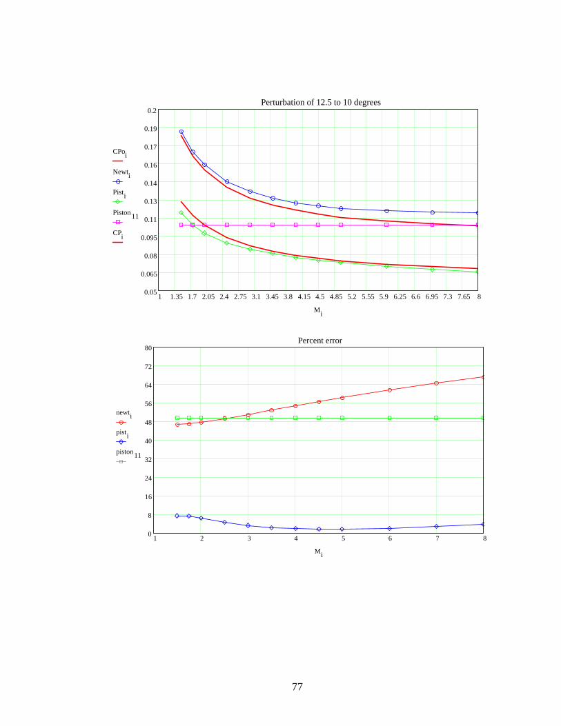
77

1 1.35 1.7 2.05 2.4 2.75 3.1 3.45 3.8 4.15 4.5 4.85 5.2 5.55 5.9 6.25 6.6 6.95 7.3 7.65 80.05

0.065

0.08

0.095

0.11

0.13

0.14

0.16

0.17

0.19

0.2Perturbation of 12.5 to 10 degrees

CPoi

Newti

Pisti

Piston11

CPi

Mi

1 2 3 4 5 6 7 80

8

16

24

32

40

48

56

64

72

80Percent error

newti

pisti

piston 11

Mi

78

1 1.35 1.7 2.05 2.4 2.75 3.1 3.45 3.8 4.15 4.5 4.85 5.2 5.55 5.9 6.25 6.6 6.95 7.3 7.65 80

0.02

0.04

0.06

0.08

0.1

0.12

0.14

0.16

0.18


CPoi

Newti

Pisti

Piston i

CPi

Mi

1 2 3 4 5 6 7 805.33

10.6716

21.3326.67

3237.3342.67

4853.3358.67

6469.3374.67

80Percent error

newt1

pisti

piston 11

Mi

79

1 1.35 1.7 2.05 2.4 2.75 3.1 3.45 3.8 4.15 4.5 4.85 5.2 5.55 5.9 6.25 6.6 6.95 7.3 7.65 80

0.01

0.03

0.04

0.056

0.07

0.084

0.098

0.11

0.13


CPoi

Newti

Pisti

Piston i

CPi

Mi

1 2 3 4 5 6 7 80

8

16

24

32

40

48

56

64

72

80

88

96

104

112

120Percent error

newt1

pisti

piston 12

Mi

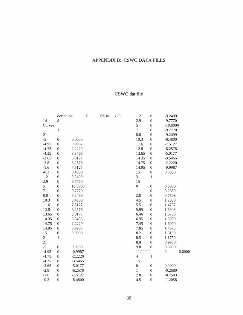
80

APPENDIX B: CSWC DATA FILES

CSWC dat file

1 definition à felisa x35 14 8 Curves 1 1 21 -5 0 0.0000 -4.95 0 0.9987 -4.75 0 2.2220 -4.35 0 3.5465 -3.65 0 5.0177 -2.8 0 6.2578 -1.6 0 7.5127 -0.3 0 8.4800 1.2 0 9.2499 2.9 0 9.7770 5 0 10.0000 7.1 0 9.7770 8.8 0 9.2499 10.3 0 8.4800 11.6 0 7.5127 12.8 0 6.2578 13.65 0 5.0177 14.35 0 3.5465 14.75 0 2.2220 14.95 0 0.9987 15 0 0.0000 2 1 21 -5 0 0.0000 -4.95 0 -0.9987 -4.75 0 -2.2220 -4.35 0 -3.5465 -3.65 0 -5.0177 -2.8 0 -6.2578 -1.6 0 -7.5127 -0.3 0 -8.4800

1.2 0 -9.2499 2.9 0 -9.7770 5 0 -10.0000 7.1 0 -9.7770 8.8 0 -9.2499 10.3 0 -8.4800 11.6 0 -7.5127 12.8 0 -6.2578 13.65 0 -5.0177 14.35 0 -3.5465 14.75 0 -2.2220 14.95 0 -0.9987 15 0 0.0000 3 1 15 0 0 0.0000 1 0 0.2680 2.8 0 0.7503 4.5 0 1.2058 5.5 0 1.4737 5.95 0 1.5943 6.46 0 1.6700 6.95 0 1.6900 7.45 0 1.6000 7.85 0 1.4675 8.2 0 1.3100 8.5 0 1.1750 8.9 0 0.9950 9.8 0 0.5900 11.11111 0 0.0000 4 1 15 0 0 0.0000 1 0 -0.2680 2.8 0 -0.7503 4.5 0 -1.2058

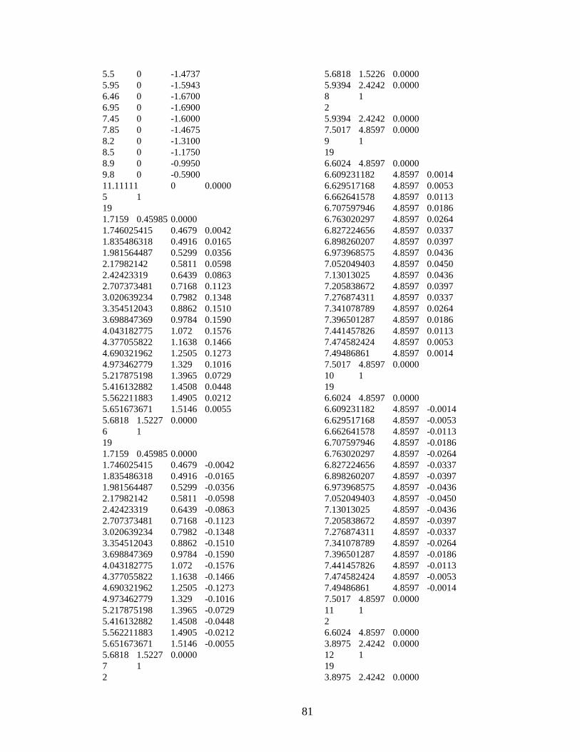
81

5.5 0 -1.4737 5.95 0 -1.5943 6.46 0 -1.6700 6.95 0 -1.6900 7.45 0 -1.6000 7.85 0 -1.4675 8.2 0 -1.3100 8.5 0 -1.1750 8.9 0 -0.9950 9.8 0 -0.5900 11.11111 0 0.0000 5 1 19 1.7159 0.45985 0.0000 1.746025415 0.4679 0.0042 1.835486318 0.4916 0.0165 1.981564487 0.5299 0.0356 2.17982142 0.5811 0.0598 2.42423319 0.6439 0.0863 2.707373481 0.7168 0.1123 3.020639234 0.7982 0.1348 3.354512043 0.8862 0.1510 3.698847369 0.9784 0.1590 4.043182775 1.072 0.1576 4.377055822 1.1638 0.1466 4.690321962 1.2505 0.1273 4.973462779 1.329 0.1016 5.217875198 1.3965 0.0729 5.416132882 1.4508 0.0448 5.562211883 1.4905 0.0212 5.651673671 1.5146 0.0055 5.6818 1.5227 0.0000 6 1 19 1.7159 0.45985 0.0000 1.746025415 0.4679 -0.0042 1.835486318 0.4916 -0.0165 1.981564487 0.5299 -0.0356 2.17982142 0.5811 -0.0598 2.42423319 0.6439 -0.0863 2.707373481 0.7168 -0.1123 3.020639234 0.7982 -0.1348 3.354512043 0.8862 -0.1510 3.698847369 0.9784 -0.1590 4.043182775 1.072 -0.1576 4.377055822 1.1638 -0.1466 4.690321962 1.2505 -0.1273 4.973462779 1.329 -0.1016 5.217875198 1.3965 -0.0729 5.416132882 1.4508 -0.0448 5.562211883 1.4905 -0.0212 5.651673671 1.5146 -0.0055 5.6818 1.5227 0.0000 7 1 2

5.6818 1.5226 0.0000 5.9394 2.4242 0.0000 8 1 2 5.9394 2.4242 0.0000 7.5017 4.8597 0.0000 9 1 19 6.6024 4.8597 0.0000 6.609231182 4.8597 0.0014 6.629517168 4.8597 0.0053 6.662641578 4.8597 0.0113 6.707597946 4.8597 0.0186 6.763020297 4.8597 0.0264 6.827224656 4.8597 0.0337 6.898260207 4.8597 0.0397 6.973968575 4.8597 0.0436 7.052049403 4.8597 0.0450 7.13013025 4.8597 0.0436 7.205838672 4.8597 0.0397 7.276874311 4.8597 0.0337 7.341078789 4.8597 0.0264 7.396501287 4.8597 0.0186 7.441457826 4.8597 0.0113 7.474582424 4.8597 0.0053 7.49486861 4.8597 0.0014 7.5017 4.8597 0.0000 10 1 19 6.6024 4.8597 0.0000 6.609231182 4.8597 -0.0014 6.629517168 4.8597 -0.0053 6.662641578 4.8597 -0.0113 6.707597946 4.8597 -0.0186 6.763020297 4.8597 -0.0264 6.827224656 4.8597 -0.0337 6.898260207 4.8597 -0.0397 6.973968575 4.8597 -0.0436 7.052049403 4.8597 -0.0450 7.13013025 4.8597 -0.0436 7.205838672 4.8597 -0.0397 7.276874311 4.8597 -0.0337 7.341078789 4.8597 -0.0264 7.396501287 4.8597 -0.0186 7.441457826 4.8597 -0.0113 7.474582424 4.8597 -0.0053 7.49486861 4.8597 -0.0014 7.5017 4.8597 0.0000 11 1 2 6.6024 4.8597 0.0000 3.8975 2.4242 0.0000 12 1 19 3.8975 2.4242 0.0000

82

3.913010498 2.4242 0.0031 3.959070716 2.4242 0.0120 4.034281138 2.4242 0.0255 4.136356539 2.4242 0.0422 4.262195413 2.4242 0.0599 4.407974218 2.4242 0.0766 4.569263545 2.4242 0.0902 4.741162707 2.4242 0.0990 4.918448645 2.4242 0.1021 5.095734625 2.4242 0.0990 5.26763391 2.4242 0.0902 5.428923436 2.4242 0.0766 5.574702511 2.4242 0.0599 5.70054172 2.4242 0.0422 5.802617507 2.4242 0.0255 5.877828358 2.4242 0.0119 5.923889031 2.4242 0.0031 5.9394 2.4242 0.0000 13 1 19 3.8975 2.4242 0.0000 3.913010498 2.4242 -0.0031 3.959070716 2.4242 -0.0120 4.034281138 2.4242 -0.0255 4.136356539 2.4242 -0.0422 4.262195413 2.4242 -0.0599 4.407974218 2.4242 -0.0766 4.569263545 2.4242 -0.0902 4.741162707 2.4242 -0.0990 4.918448645 2.4242 -0.1021 5.095734625 2.4242 -0.0990 5.26763391 2.4242 -0.0902 5.428923436 2.4242 -0.0766 5.574702511 2.4242 -0.0599 5.70054172 2.4242 -0.0422 5.802617507 2.4242 -0.0255 5.877828358 2.4242 -0.0119 5.923889031 2.4242 -0.0031 5.9394 2.4242 0.0000 14 1 2 1.7159 0.4598 0.0000 3.8975 2.4242 0.0000 Surfaces 1 1 21 2 -5 0 0.0000 -4.95 0 0.9987 -4.75 0 2.2220 -4.35 0 3.5465 -3.65 0 5.0177 -2.8 0 6.2578 -1.6 0 7.5127 -0.3 0 8.4800 1.2 0 9.2499

2.9 0 9.7770 5 0 10.0000 7.1 0 9.7770 8.8 0 9.2499 10.3 0 8.4800 11.6 0 7.5127 12.8 0 6.2578 13.65 0 5.0177 14.35 0 3.5465 14.75 0 2.2220 14.95 0 0.9987 15 0 0.0000 -5 0 0.0000 -4.95 0 -0.9987 -4.75 0 -2.2220 -4.35 0 -3.5465 -3.65 0 -5.0177 -2.8 0 -6.2578 -1.6 0 -7.5127 -0.3 0 -8.4800 1.2 0 -9.2499 2.9 0 -9.7770 5 0 -10.0000 7.1 0 -9.7770 8.8 0 -9.2499 10.3 0 -8.4800 11.6 0 -7.5127 12.8 0 -6.2578 13.65 0 -5.0177 14.35 0 -3.5465 14.75 0 -2.2220 14.95 0 -0.9987 15 0 0.0000 2 1 21 21 -5 0 0.0000 -4.95 0 0.9987 -4.75 0 2.2220 -4.35 0 3.5465 -3.65 0 5.0177 -2.8 0 6.2578 -1.6 0 7.5127 -0.3 0 8.4800 1.2 0 9.2499 2.9 0 9.7770 5 0 10.0000 7.1 0 9.7770 8.8 0 9.2499 10.3 0 8.4800 11.6 0 7.5127 12.8 0 6.2578 13.65 0 5.0177 14.35 0 3.5465 14.75 0 2.2220 14.95 0 0.9987

83

15 0 0.0000 -5 0 0.0000 -4.95 0.156238669 0.9865 -4.75 0.347604694 2.1947 -4.35 0.554790787 3.5028 -3.65 0.784943468 4.9559 -2.8 0.978934015 6.1808 -1.6 1.175237336 7.4202 -0.3 1.326559463 8.3756 1.2 1.44699645 9.1360 2.9 1.529460651 9.6566 5 1.56434334 9.8769 7.1 1.529460651 9.6566 8.8 1.44699645 9.1360 10.3 1.326559463 8.3756 11.6 1.175237336 7.4202 12.8 0.978934015 6.1808 13.65 0.784943468 4.9559 14.35 0.554790787 3.5028 14.75 0.347604694 2.1947 14.95 0.156238669 0.9865 15 0 0.0000 -5 0 0.0000 -4.95 0.308630229 0.9499 -4.75 0.68665022 2.1133 -4.35 1.095920807 3.3729 -3.65 1.550559056 4.7721 -2.8 1.933763466 5.9515 -1.6 2.321536477 7.1450 -0.3 2.620454684 8.0649 1.2 2.858363104 8.7971 2.9 3.021260969 9.2985 5 3.09016742 9.5106 7.1 3.021260969 9.2985 8.8 2.858363104 8.7971 10.3 2.620454684 8.0649 11.6 2.321536477 7.1450 12.8 1.933763466 5.9515 13.65 1.550559056 4.7721 14.35 1.095920807 3.3729 14.75 0.68665022 2.1133 14.95 0.308630229 0.9499 15 0 0.0000 -5 0 0.0000 -4.95 0.453422302 0.8899 -4.75 1.008788168 1.9799 -4.35 1.610065665 3.1599 -3.65 2.277994798 4.4708 -2.8 2.840977323 5.5757 -1.6 3.410671782 6.6938 -0.3 3.849825723 7.5557 1.2 4.199347492 8.2417 2.9 4.43866794 8.7114 5 4.539901451 8.9101 7.1 4.43866794 8.7114

8.8 4.199347492 8.2417 10.3 3.849825723 7.5557 11.6 3.410671782 6.6938 12.8 2.840977323 5.5757 13.65 2.277994798 4.4708 14.35 1.610065665 3.1599 14.75 1.008788168 1.9799 14.95 0.453422302 0.8899 15 0 0.0000 -5 0 0.0000 -4.95 0.587049632 0.8080 -4.75 1.306086445 1.7977 -4.35 2.084565429 2.8692 -3.65 2.949338842 4.0594 -2.8 3.678237008 5.0627 -1.6 4.41582517 6.0779 -0.3 4.984401436 6.8604 1.2 5.436930181 7.4833 2.9 5.74678036 7.9098 5 5.877848229 8.0902 7.1 5.74678036 7.9098 8.8 5.436930181 7.4833 10.3 4.984401436 6.8604 11.6 4.41582517 6.0779 12.8 3.678237008 5.0627 13.65 2.949338842 4.0594 14.35 2.084565429 2.8692 14.75 1.306086445 1.7977 14.95 0.587049632 0.8080 15 0 0.0000 -5 0 0.0000 -4.95 0.706221876 0.7062 -4.75 1.571224594 1.5712 -4.35 2.507736361 2.5077 -3.65 3.548060498 3.5481 -2.8 4.424926442 4.4249 -1.6 5.31224647 5.3123 -0.3 5.996244849 5.9963 1.2 6.540637831 6.5406 2.9 6.913388213 6.9134 5 7.071063121 7.0711 7.1 6.913388213 6.9134 8.8 6.540637831 6.5406 10.3 5.996244849 5.9963 11.6 5.31224647 5.3123 12.8 4.424926442 4.4249 13.65 3.548060498 3.5481 14.35 2.507736361 2.5077 14.75 1.571224594 1.5712 14.95 0.706221876 0.7062 15 0 0.0000 -5 0 0.0000 -4.95 0.808004623 0.5871 -4.75 1.797674043 1.3061 -4.35 2.869158605 2.0846

84

-3.65 4.059417277 2.9493 -2.8 5.062659686 3.6782 -1.6 6.077862852 4.4158 -0.3 6.860441064 4.9844 1.2 7.483293542 5.4369 2.9 7.909765791 5.7468 5 8.090165265 5.8779 7.1 7.909765791 5.7468 8.8 7.483293542 5.4369 10.3 6.860441064 4.9844 11.6 6.077862852 4.4158 12.8 5.062659686 3.6782 13.65 4.059417277 2.9493 14.35 2.869158605 2.0846 14.75 1.797674043 1.3061 14.95 0.808004623 0.5871 15 0 0.0000 -5 0 0.0000 -4.95 0.889891648 0.4534 -4.75 1.979858867 1.0088 -4.35 3.159932761 1.6101 -3.65 4.470817898 2.2780 -2.8 5.575733657 2.8410 -1.6 6.693822332 3.4107 -0.3 7.555710735 3.8498 1.2 8.241686041 4.1994 2.9 8.711379013 4.4387 5 8.910061025 4.5399 7.1 8.711379013 4.4387 8.8 8.241686041 4.1994 10.3 7.555710735 3.8498 11.6 6.693822332 3.4107 12.8 5.575733657 2.8410 13.65 4.470817898 2.2780 14.35 3.159932761 1.6101 14.75 1.979858867 1.0088 14.95 0.889891648 0.4534 15 0 0.0000 -5 0 0.0000 -4.95 0.949866624 0.3086 -4.75 2.113293076 0.6867 -4.35 3.372899017 1.0959 -3.65 4.77213233 1.5506 -2.8 5.951514792 1.9338 -1.6 7.144957968 2.3215 -0.3 8.064934046 2.6205 1.2 8.79714122 2.8584 2.9 9.298489534 3.0213 5 9.510561883 3.0902 7.1 9.298489534 3.0213 8.8 8.79714122 2.8584 10.3 8.064934046 2.6205 11.6 7.144957968 2.3215 12.8 5.951514792 1.9338 13.65 4.77213233 1.5506

14.35 3.372899017 1.0959 14.75 2.113293076 0.6867 14.95 0.949866624 0.3086 15 0 0.0000 -5 0 0.0000 -4.95 0.986452771 0.1562 -4.75 2.194691084 0.3476 -4.35 3.502813444 0.5548 -3.65 4.955941225 0.7850 -2.8 6.180750128 0.9789 -1.6 7.420161323 1.1752 -0.3 8.37557225 1.3266 1.2 9.13598195 1.4470 2.9 9.656640768 1.5295 5 9.876881538 1.5644 7.1 9.656640768 1.5295 8.8 9.13598195 1.4470 10.3 8.37557225 1.3266 11.6 7.420161323 1.1752 12.8 6.180750128 0.9789 13.65 4.955941225 0.7850 14.35 3.502813444 0.5548 14.75 2.194691084 0.3476 14.95 0.986452771 0.1562 15 0 0.0000 -5 0 0.0000 -4.95 0.998749218 0.0000 -4.75 2.222048604 0.0000 -4.35 3.546477125 0.0000 -3.65 5.017718605 0.0000 -2.8 6.257795139 0.0000 -1.6 7.512655988 0.0000 -0.3 8.479976415 0.0000 1.2 9.249864864 0.0000 2.9 9.777013859 0.0000 5 10 0.0000 7.1 9.777013859 0.0000 8.8 9.249864864 0.0000 10.3 8.479976415 0.0000 11.6 7.512655988 0.0000 12.8 6.257795139 0.0000 13.65 5.017718605 0.0000 14.35 3.546477125 0.0000 14.75 2.222048604 0.0000 14.95 0.998749218 0.0000 15 0 0.0000 -5 0 0.0000 -4.95 0.986453186 -0.1562 -4.75 2.194692006 -0.3476 -4.35 3.502814917 -0.5548 -3.65 4.955943308 -0.7849 -2.8 6.180752725 -0.9789 -1.6 7.420164442 -1.1752 -0.3 8.37557577 -1.3265 1.2 9.13598579 -1.4470

85

2.9 9.656644827 -1.5294 5 9.876885689 -1.5643 7.1 9.656644827 -1.5294 8.8 9.13598579 -1.4470 10.3 8.37557577 -1.3265 11.6 7.420164442 -1.1752 12.8 6.180752725 -0.9789 13.65 4.955943308 -0.7849 14.35 3.502814917 -0.5548 14.75 2.194692006 -0.3476 14.95 0.986453186 -0.1562 15 0 0.0000 -5 0 0.0000 -4.95 0.949867443 -0.3086 -4.75 2.113294898 -0.6866 -4.35 3.372901925 -1.0959 -3.65 4.772136445 -1.5506 -2.8 5.951519923 -1.9338 -1.6 7.144964129 -2.3215 -0.3 8.064941 -2.6204 1.2 8.797148805 -2.8584 2.9 9.298497551 -3.0212 5 9.510570083 -3.0902 7.1 9.298497551 -3.0212 8.8 8.797148805 -2.8584 10.3 8.064941 -2.6204 11.6 7.144964129 -2.3215 12.8 5.951519923 -1.9338 13.65 4.772136445 -1.5506 14.35 3.372901925 -1.0959 14.75 2.113294898 -0.6866 14.95 0.949867443 -0.3086 15 0 0.0000 -5 0 0.0000 -4.95 0.889892851 -0.4534 -4.75 1.979861544 -1.0088 -4.35 3.159937034 -1.6101 -3.65 4.470823943 -2.2780 -2.8 5.575741196 -2.8410 -1.6 6.693831382 -3.4107 -0.3 7.555720951 -3.8498 1.2 8.241697185 -4.1993 2.9 8.711390791 -4.4387 5 8.910073072 -4.5399 7.1 8.711390791 -4.4387 8.8 8.241697185 -4.1993 10.3 7.555720951 -3.8498 11.6 6.693831382 -3.4107 12.8 5.575741196 -2.8410 13.65 4.470823943 -2.2780 14.35 3.159937034 -1.6101 14.75 1.979861544 -1.0088 14.95 0.889892851 -0.4534 15 0 0.0000 -5 0 0.0000

-4.95 0.808006181 -0.5870 -4.75 1.797677509 -1.3061 -4.35 2.869164137 -2.0846 -3.65 4.059425103 -2.9493 -2.8 5.062669447 -3.6782 -1.6 6.07787457 -4.4158 -0.3 6.86045429 -4.9844 1.2 7.48330797 -5.4369 2.9 7.909781041 -5.7468 5 8.090180862 -5.8778 7.1 7.909781041 -5.7468 8.8 7.48330797 -5.4369 10.3 6.86045429 -4.9844 11.6 6.07787457 -4.4158 12.8 5.062669447 -3.6782 13.65 4.059425103 -2.9493 14.35 2.869164137 -2.0846 14.75 1.797677509 -1.3061 14.95 0.808006181 -0.5870 15 0 0.0000 -5 0 0.0000 -4.95 0.70622375 -0.7062 -4.75 1.571228763 -1.5712 -4.35 2.507743015 -2.5077 -3.65 3.548069913 -3.5481 -2.8 4.424938184 -4.4249 -1.6 5.312260567 -5.3122 -0.3 5.996260761 -5.9962 1.2 6.540655187 -6.5406 2.9 6.913406558 -6.9134 5 7.071081885 -7.0711 7.1 6.913406558 -6.9134 8.8 6.540655187 -6.5406 10.3 5.996260761 -5.9962 11.6 5.312260567 -5.3122 12.8 4.424938184 -4.4249 13.65 3.548069913 -3.5481 14.35 2.507743015 -2.5077 14.75 1.571228763 -1.5712 14.95 0.70622375 -0.7062 15 0 0.0000 -5 0 0.0000 -4.95 0.587051776 -0.8080 -4.75 1.306091216 -1.7977 -4.35 2.084573043 -2.8692 -3.65 2.949349614 -4.0594 -2.8 3.678250442 -5.0627 -1.6 4.415841298 -6.0779 -0.3 4.98441964 -6.8604 1.2 5.436950039 -7.4833 2.9 5.746801349 -7.9098 5 5.877869697 -8.0902 7.1 5.746801349 -7.9098 8.8 5.436950039 -7.4833 10.3 4.98441964 -6.8604

86

11.6 4.415841298 -6.0779 12.8 3.678250442 -5.0627 13.65 2.949349614 -4.0594 14.35 2.084573043 -2.8692 14.75 1.306091216 -1.7977 14.95 0.587051776 -0.8080 15 0 0.0000 -5 0 0.0000 -4.95 0.453424664 -0.8899 -4.75 1.008793422 -1.9799 -4.35 1.61007405 -3.1599 -3.65 2.278006661 -4.4708 -2.8 2.840992119 -5.5757 -1.6 3.410689545 -6.6938 -0.3 3.849845773 -7.5557 1.2 4.199369362 -8.2417 2.9 4.438691057 -8.7114 5 4.539925094 -8.9101 7.1 4.438691057 -8.7114 8.8 4.199369362 -8.2417 10.3 3.849845773 -7.5557 11.6 3.410689545 -6.6938 12.8 2.840992119 -5.5757 13.65 2.278006661 -4.4708 14.35 1.61007405 -3.1599 14.75 1.008793422 -1.9799 14.95 0.453424664 -0.8899 15 0 0.0000 -5 0 0.0000 -4.95 0.30863275 -0.9499 -4.75 0.686655828 -2.1133 -4.35 1.095929757 -3.3729 -3.65 1.550571719 -4.7721 -2.8 1.933779259 -5.9515 -1.6 2.321555437 -7.1450 -0.3 2.620476085 -8.0649 1.2 2.858386448 -8.7971 2.9 3.021285644 -9.2985 5 3.090192657 -9.5106 7.1 3.021285644 -9.2985 8.8 2.858386448 -8.7971 10.3 2.620476085 -8.0649 11.6 2.321555437 -7.1450 12.8 1.933779259 -5.9515 13.65 1.550571719 -4.7721 14.35 1.095929757 -3.3729 14.75 0.686655828 -2.1133 14.95 0.30863275 -0.9499 15 0 0.0000 -5 0 0.0000 -4.95 0.156241286 -0.9865 -4.75 0.347610517 -2.1947 -4.35 0.554800082 -3.5028 -3.65 0.784956619 -4.9559 -2.8 0.978950416 -6.1807

-1.6 1.175257026 -7.4202 -0.3 1.326581688 -8.3756 1.2 1.447020693 -9.1360 2.9 1.529486276 -9.6566 5 1.564369549 -9.8769 7.1 1.529486276 -9.6566 8.8 1.447020693 -9.1360 10.3 1.326581688 -8.3756 11.6 1.175257026 -7.4202 12.8 0.978950416 -6.1807 13.65 0.784956619 -4.9559 14.35 0.554800082 -3.5028 14.75 0.347610517 -2.1947 14.95 0.156241286 -0.9865 15 0 0.0000 -5 0 0.0000 -4.95 0 -0.9987 -4.75 0 -2.2220 -4.35 0 -3.5465 -3.65 0 -5.0177 -2.8 0 -6.2578 -1.6 0 -7.5127 -0.3 0 -8.4800 1.2 0 -9.2499 2.9 0 -9.7770 5 0 -10.0000 7.1 0 -9.7770 8.8 0 -9.2499 10.3 0 -8.4800 11.6 0 -7.5127 12.8 0 -6.2578 13.65 0 -5.0177 14.35 0 -3.5465 14.75 0 -2.2220 14.95 0 -0.9987 15 0 0.0000 3 1 15 16 0 0 0.0000 1 0 0.2680 2.8 0 0.7503 4.5 0 1.2058 5.5 0 1.4737 5.95 0 1.5943 6.46 0 1.6700 6.95 0 1.6900 7.45 0 1.6000 7.85 0 1.4675 8.2 0 1.3100 8.5 0 1.1750 8.9 0 0.9950 9.8 0 0.5900 11.11111 0 0.0000 0 0 0.0000 1 0.055709891 0.2621

87

2.8 0.155987695 0.7339 4.5 0.25069451 1.1794 5.5 0.306404402 1.4415 5.95 0.331473853 1.5595 6.46 0.347212235 1.6335 6.95 0.351370465 1.6531 7.45 0.332658428 1.5650 7.85 0.305110152 1.4354 8.2 0.272364088 1.2814 8.5 0.244296033 1.1493 8.9 0.20687196 0.9733 9.8 0.122667795 0.5771 11.11111 0 0.0000 0 0 0.0000 1 0.108984997 0.2448 2.8 0.305157991 0.6854 4.5 0.490432486 1.1015 5.5 0.599417483 1.3463 5.95 0.648460732 1.4565 6.46 0.679249654 1.5256 6.95 0.687384381 1.5439 7.45 0.650778112 1.4617 7.85 0.596885549 1.3406 8.2 0.532824579 1.1967 8.5 0.477915176 1.0734 8.9 0.404702638 0.9090 9.8 0.239974429 0.5390 11.11111 0 0.0000 0 0 0.0000 1 0.157496943 0.2168 2.8 0.440991441 0.6070 4.5 0.708736245 0.9755 5.5 0.866233188 1.1923 5.95 0.937106813 1.2898 6.46 0.981600654 1.3511 6.95 0.993356351 1.3672 7.45 0.940455717 1.2944 7.85 0.862574228 1.1872 8.2 0.769998118 1.0598 8.5 0.690647167 0.9506 8.9 0.584845899 0.8050 9.8 0.346793046 0.4773 11.11111 0 0.0000 0 0 0.0000 1 0.199125529 0.1793 2.8 0.557551482 0.5020 4.5 0.896064881 0.8068 5.5 1.09519041 0.9861 5.95 1.184796898 1.0668 6.46 1.241051068 1.1174 6.95 1.255913955 1.1308 7.45 1.189030963 1.0706 7.85 1.090564337 0.9819 8.2 0.973519101 0.8766 8.5 0.873194614 0.7862

8.9 0.73942863 0.6658 9.8 0.438455168 0.3948 11.11111 0 0.0000 0 0 0.0000 1 0.232051388 0.1340 2.8 0.649743888 0.3751 4.5 1.044231248 0.6029 5.5 1.276282636 0.7369 5.95 1.380705761 0.7972 6.46 1.446261686 0.8350 6.95 1.463582185 0.8450 7.45 1.385639938 0.8000 7.85 1.270891631 0.7338 8.2 1.1344927 0.6550 8.5 1.01757933 0.5875 8.9 0.861694837 0.4975 9.8 0.510954727 0.2950 11.11111 0 0.0000 0 0 0.0000 1 0.254835506 0.0828 2.8 0.713539416 0.2318 4.5 1.146759775 0.3726 5.5 1.401595281 0.4554 5.95 1.516271259 0.4927 6.46 1.588263834 0.5161 6.95 1.607284958 0.5222 7.45 1.521689901 0.4944 7.85 1.395674956 0.4535 8.2 1.245883607 0.4048 8.5 1.117491021 0.3631 8.9 0.946300907 0.3075 9.8 0.561123151 0.1823 11.11111 0 0.0000 0 0 0.0000 1 0.266482107 0.0280 2.8 0.7461499 0.0784 4.5 1.199169482 0.1260 5.5 1.465651589 0.1540 5.95 1.585568538 0.1667 6.46 1.660851349 0.1746 6.95 1.680741784 0.1767 7.45 1.591234825 0.1672 7.85 1.459460691 0.1534 8.2 1.302823513 0.1369 8.5 1.168563075 0.1228 8.9 0.989549157 0.1040 9.8 0.586767842 0.0617 11.11111 0 0.0000 0 0 0.0000 1 0.266482182 -0.0280 2.8 0.746150108 -0.0784 4.5 1.199169817 -0.1260 5.5 1.465651998 -0.1540 5.95 1.58556898 -0.1666 6.46 1.660851812 -0.1746

88

6.95 1.680742253 -0.1767 7.45 1.591235269 -0.1672 7.85 1.459461099 -0.1534 8.2 1.302823877 -0.1369 8.5 1.168563401 -0.1228 8.9 0.989549433 -0.1040 9.8 0.586768006 -0.0617 11.11111 0 0.0000 0 0 0.0000 1 0.254835725 -0.0828 2.8 0.713540031 -0.2318 4.5 1.146760764 -0.3726 5.5 1.40159649 -0.4554 5.95 1.516272566 -0.4927 6.46 1.588265204 -0.5161 6.95 1.607286344 -0.5222 7.45 1.521691213 -0.4944 7.85 1.39567616 -0.4535 8.2 1.245884681 -0.4048 8.5 1.117491985 -0.3631 8.9 0.946301723 -0.3075 9.8 0.561123635 -0.1823 11.11111 0 0.0000 0 0 0.0000 1 0.232051744 -0.1340 2.8 0.649744883 -0.3751 4.5 1.044232848 -0.6029 5.5 1.276284592 -0.7369 5.95 1.380707877 -0.7971 6.46 1.446263901 -0.8350 6.95 1.463584427 -0.8450 7.45 1.385642061 -0.8000 7.85 1.270893578 -0.7337 8.2 1.134494438 -0.6550 8.5 1.017580889 -0.5875 8.9 0.861696157 -0.4975 9.8 0.51095551 -0.2950 11.11111 0 0.0000 0 0 0.0000 1 0.199126005 -0.1793 2.8 0.557552814 -0.5020 4.5 0.896067022 -0.8068 5.5 1.095193027 -0.9861 5.95 1.184799729 -1.0668 6.46 1.241054033 -1.1174 6.95 1.255916956 -1.1308 7.45 1.189033804 -1.0706 7.85 1.090566942 -0.9819 8.2 0.973521427 -0.8766 8.5 0.8731967 -0.7862 8.9 0.739430397 -0.6658 9.8 0.438456215 -0.3948 11.11111 0 0.0000 0 0 0.0000 1 0.157497519 -0.2168

2.8 0.440993052 -0.6070 4.5 0.708738833 -0.9755 5.5 0.866236352 -1.1923 5.95 0.937110235 -1.2898 6.46 0.981604239 -1.3511 6.95 0.993359979 -1.3672 7.45 0.940459152 -1.2944 7.85 0.862577378 -1.1872 8.2 0.77000093 -1.0598 8.5 0.690649689 -0.9506 8.9 0.584848035 -0.8050 9.8 0.346794312 -0.4773 11.11111 0 0.0000 0 0 0.0000 1 0.108985646 -0.2448 2.8 0.30515981 -0.6854 4.5 0.490435409 -1.1015 5.5 0.599421056 -1.3463 5.95 0.648464596 -1.4565 6.46 0.679253703 -1.5256 6.95 0.687388477 -1.5439 7.45 0.65078199 -1.4617 7.85 0.596889107 -1.3406 8.2 0.532827755 -1.1967 8.5 0.477918024 -1.0734 8.9 0.40470505 -0.9090 9.8 0.239975859 -0.5390 11.11111 0 0.0000 0 0 0.0000 1 0.055710587 -0.2621 2.8 0.155989643 -0.7339 4.5 0.25069764 -1.1794 5.5 0.306408227 -1.4415 5.95 0.331477991 -1.5595 6.46 0.347216569 -1.6335 6.95 0.351374852 -1.6531 7.45 0.332662581 -1.5650 7.85 0.305113961 -1.4354 8.2 0.272367489 -1.2814 8.5 0.244299083 -1.1493 8.9 0.206874543 -0.9733 9.8 0.122669327 -0.5771 11.11111 0 0.0000 0 0 0.0000 1 0 -0.2680 2.8 0 -0.7503 4.5 0 -1.2058 5.5 0 -1.4737 5.95 0 -1.5943 6.46 0 -1.6700 6.95 0 -1.6900 7.45 0 -1.6000 7.85 0 -1.4675 8.2 0 -1.3100 8.5 0 -1.1750

89

8.9 0 -0.9950 9.8 0 -0.5900 11.11111 0 0.0000 4 1 19 2 1.7159 0.45985 0.0000 1.746025415 0.4679 0.0042 1.835486318 0.4916 0.0165 1.981564487 0.5299 0.0356 2.17982142 0.5811 0.0598 2.42423319 0.6439 0.0863 2.707373481 0.7168 0.1123 3.020639234 0.7982 0.1348 3.354512043 0.8862 0.1510 3.698847369 0.9784 0.1590 4.043182775 1.072 0.1576 4.377055822 1.1638 0.1466 4.690321962 1.2505 0.1273 4.973462779 1.329 0.1016 5.217875198 1.3965 0.0729 5.416132882 1.4508 0.0448 5.562211883 1.4905 0.0212 5.651673671 1.5146 0.0055 5.6818 1.5227 0.0000 3.8975 2.4242 0.0000 3.913010498 2.4242 0.0031 3.959070716 2.4242 0.0120 4.034281138 2.4242 0.0255 4.136356539 2.4242 0.0422 4.262195413 2.4242 0.0599 4.407974218 2.4242 0.0766 4.569263545 2.4242 0.0902 4.741162707 2.4242 0.0990 4.918448645 2.4242 0.1021 5.095734625 2.4242 0.0990 5.26763391 2.4242 0.0902 5.428923436 2.4242 0.0766 5.574702511 2.4242 0.0599 5.70054172 2.4242 0.0422 5.802617507 2.4242 0.0255 5.877828358 2.4242 0.0119 5.923889031 2.4242 0.0031 5.9394 2.4242 0.0000 5 1 2 2 6.6024 4.8597 1.0000 7.5017 4.8597 1.0000 6.6024 4.8597 -1.0000 7.5017 4.8597 -1.0000 6 1 19 2 6.6024 4.8597 0.0000 6.609231182 4.8597 -0.0014 6.629517168 4.8597 -0.0053 6.662641578 4.8597 -0.0113

6.707597946 4.8597 -0.0186 6.763020297 4.8597 -0.0264 6.827224656 4.8597 -0.0337 6.898260207 4.8597 -0.0397 6.973968575 4.8597 -0.0436 7.052049403 4.8597 -0.0450 7.13013025 4.8597 -0.0436 7.205838672 4.8597 -0.0397 7.276874311 4.8597 -0.0337 7.341078789 4.8597 -0.0264 7.396501287 4.8597 -0.0186 7.441457826 4.8597 -0.0113 7.474582424 4.8597 -0.0053 7.49486861 4.8597 -0.0014 7.5017 4.8597 0.0000 3.8975 2.4242 0.0000 3.913010498 2.4242 -0.0031 3.959070716 2.4242 -0.0120 4.034281138 2.4242 -0.0255 4.136356539 2.4242 -0.0422 4.262195413 2.4242 -0.0599 4.407974218 2.4242 -0.0766 4.569263545 2.4242 -0.0902 4.741162707 2.4242 -0.0990 4.918448645 2.4242 -0.1021 5.095734625 2.4242 -0.0990 5.26763391 2.4242 -0.0902 5.428923436 2.4242 -0.0766 5.574702511 2.4242 -0.0599 5.70054172 2.4242 -0.0422 5.802617507 2.4242 -0.0255 5.877828358 2.4242 -0.0119 5.923889031 2.4242 -0.0031 5.9394 2.4242 0.0000 7 1 19 2 3.8975 2.4242 0.0000 3.913010498 2.4242 0.0031 3.959070716 2.4242 0.0120 4.034281138 2.4242 0.0255 4.136356539 2.4242 0.0422 4.262195413 2.4242 0.0599 4.407974218 2.4242 0.0766 4.569263545 2.4242 0.0902 4.741162707 2.4242 0.0990 4.918448645 2.4242 0.1021 5.095734625 2.4242 0.0990 5.26763391 2.4242 0.0902 5.428923436 2.4242 0.0766 5.574702511 2.4242 0.0599 5.70054172 2.4242 0.0422 5.802617507 2.4242 0.0255 5.877828358 2.4242 0.0119 5.923889031 2.4242 0.0031 5.9394 2.4242 0.0000

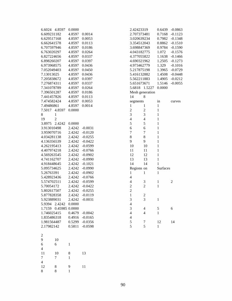
90

6.6024 4.8597 0.0000 6.609231182 4.8597 0.0014 6.629517168 4.8597 0.0053 6.662641578 4.8597 0.0113 6.707597946 4.8597 0.0186 6.763020297 4.8597 0.0264 6.827224656 4.8597 0.0337 6.898260207 4.8597 0.0397 6.973968575 4.8597 0.0436 7.052049403 4.8597 0.0450 7.13013025 4.8597 0.0436 7.205838672 4.8597 0.0397 7.276874311 4.8597 0.0337 7.341078789 4.8597 0.0264 7.396501287 4.8597 0.0186 7.441457826 4.8597 0.0113 7.474582424 4.8597 0.0053 7.49486861 4.8597 0.0014 7.5017 4.8597 0.0000 8 1 19 2 3.8975 2.4242 0.0000 3.913010498 2.4242 -0.0031 3.959070716 2.4242 -0.0120 4.034281138 2.4242 -0.0255 4.136356539 2.4242 -0.0422 4.262195413 2.4242 -0.0599 4.407974218 2.4242 -0.0766 4.569263545 2.4242 -0.0902 4.741162707 2.4242 -0.0990 4.918448645 2.4242 -0.1021 5.095734625 2.4242 -0.0990 5.26763391 2.4242 -0.0902 5.428923436 2.4242 -0.0766 5.574702511 2.4242 -0.0599 5.70054172 2.4242 -0.0422 5.802617507 2.4242 -0.0255 5.877828358 2.4242 -0.0119 5.923889031 2.4242 -0.0031 5.9394 2.4242 0.0000 1.7159 0.45985 0.0000 1.746025415 0.4679 -0.0042 1.835486318 0.4916 -0.0165 1.981564487 0.5299 -0.0356 2.17982142 0.5811 -0.0598

2.42423319 0.6439 -0.0863 2.707373481 0.7168 -0.1123 3.020639234 0.7982 -0.1348 3.354512043 0.8862 -0.1510 3.698847369 0.9784 -0.1590 4.043182775 1.072 -0.1576 4.377055822 1.1638 -0.1466 4.690321962 1.2505 -0.1273 4.973462779 1.329 -0.1016 5.217875198 1.3965 -0.0729 5.416132882 1.4508 -0.0448 5.562211883 1.4905 -0.0212 5.651673671 1.5146 -0.0055 5.6818 1.5227 0.0000 Mesh generation 14 8 segments in curves 1 1 1 2 2 1 3 3 1 4 4 1 5 5 1 6 6 1 7 7 1 8 8 1 9 9 1 10 10 1 11 11 1 12 12 1 13 13 1 14 14 1 Regions on Surfaces 1 1 1 4 4 3 1 2 2 2 1 2 1 2 3 3 1 4 3 4 5 6 4 4 1 4 5 7 12 14 5 5 1

2 9 10 6 6 1 4 11 10 8 13 7 7 1 4 12 8 9 11 8 8 1

91

4 13 7 6 14

92

CSWC Boundary Condition File

CSWC Boundary Condition File 8 14 Surface Regions 1 1 2 3 3 1 4 1 5 1 6 1 7 1 8 1 Curve Segments 1 0 2 0 3 0 4 0 5 0 6 0 7 0 8 0 9 0 10 0 11 0 12 0 13 0 14 0

93

CSWC Background File

background Mesh......X-35 4 1 1 4 0 1 -20 -5 -20 1 0 0 1.00 0 1 0 1.00 0 0 1 1.00 2 20 -5 -20 1 0 0 1.00 0 1 0 1.00 0 0 1 1.00 3 5 -5 20 1 0 0 1.00 0 1 0 1.00 0 0 1 1.00 4 5 20 0 1 0 0 1.00 0 1 0 1.00 0 0 1 1.00 1 1 2 3 4 * Point Sources 2.-Shock catcher 0.3 0.08 0 0.05 0.20 1.1 * Line Sources Leading Edge of the wing from point 1->3 1.7159 0.4598 0.00 0.08 0.24 1.36 3.8975 2.4242 0.00 0.08 0.24 1.20 Leading Edge of the wing from point 3->5 3.8975 2.4242 0.00 0.08 0.24 1.20 6.6024 4.8597 0.00 0.08 0.24 0.56 Trailing Edge of the wing from point 4->6 5.9394 2.4242 0.00 0.08 0.24 0.56 7.5017 4.8597 0.00 0.08 0.24 0.40 Trailing Edge of the wing from point 2->4 5.6818 1.5226 0.00 0.08 0.24 0.72 5.9394 2.4242 0.00 0.08 0.24 0.72 * Triangle sources

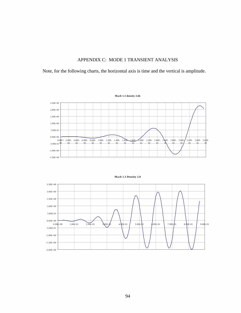
94

APPENDIX C: MODE 1 TRANSIENT ANALYSIS

Note, for the following charts, the horizontal axis is time and the vertical is amplitude.

Mach 1.3 density 2.66

-1.50E+00

-1.00E+00

-5.00E-01

0.00E+00

5.00E-01

1.00E+00

1.50E+00

2.00E+00

2.50E+00

0.00E+00

2.00E-02

4.00E-02

6.00E-02

8.00E-02

1.00E-01

1.20E-01

1.40E-01

1.60E-01

1.80E-01

2.00E-01

2.20E-01

2.40E-01

2.60E-01

2.80E-01

3.00E-01

3.20E-01

3.40E-01

3.60E-01

Mach 1.3 Density 2.0

-2.00E+00

-1.50E+00

-1.00E+00

-5.00E-01

0.00E+00

5.00E-01

1.00E+00

1.50E+00

2.00E+00

2.50E+00

0.00E+00 1.00E-01 2.00E-01 3.00E-01 4.00E-01 5.00E-01 6.00E-01 7.00E-01 8.00E-01 9.00E-01

95


-3.00E-01

-2.50E-01

-2.00E-01

-1.50E-01

-1.00E-01

-5.00E-02

0.00E+00

5.00E-02

1.00E-01

1.50E-01

2.00E-01

0.00E+00 5.00E-02 1.00E-01 1.50E-01 2.00E-01 2.50E-01 3.00E-01 3.50E-01 4.00E-01 4.50E-01 5.00E-01


0.00E+00

2.00E-03

4.00E-03

6.00E-03

8.00E-03

1.00E-02

1.20E-02

1.40E-02

1.60E-02

1.80E-02

2.00E-02

2.20E-02

0.00E+00

5.00E-02

1.00E-01

1.50E-01

2.00E-01

2.50E-01

3.00E-01

3.50E-01

4.00E-01

4.50E-01

5.00E-01

5.50E-01

6.00E-01

6.50E-01

7.00E-01

7.50E-01

8.00E-01

8.50E-01

9.00E-01

96


-1.80E-01

-1.60E-01

-1.40E-01

-1.20E-01

-1.00E-01

-8.00E-02

-6.00E-02

-4.00E-02

-2.00E-02

0.00E+00

2.00E-02

4.00E-02

6.00E-02

8.00E-02

0.00E+00 5.00E-02 1.00E-01 1.50E-01 2.00E-01 2.50E-01 3.00E-01 3.50E-01 4.00E-01 4.50E-01 5.00E-01 5.50E-01 6.00E-01 6.50E-01


-2.00E-01

-1.50E-01

-1.00E-01

-5.00E-02

0.00E+00

5.00E-02

1.00E-01

0.00E+00 5.00E-02 1.00E-01 1.50E-01 2.00E-01 2.50E-01 3.00E-01 3.50E-01 4.00E-01 4.50E-01 5.00E-01 5.50E-01 6.00E-01 6.50E-01

97


-1.40E-01

-1.20E-01

-1.00E-01

-8.00E-02

-6.00E-02

-4.00E-02

-2.00E-02

0.00E+00

2.00E-02

4.00E-02

6.00E-02

8.00E-02

0.00E+00

5.00E-02

1.00E-01

1.50E-01

2.00E-01

2.50E-01

3.00E-01

3.50E-01

4.00E-01

4.50E-01

5.00E-01

5.50E-01

6.00E-01

6.50E-01

7.00E-01

7.50E-01

8.00E-01

8.50E-01

9.00E-01

9.50E-01

1.00E+00


-2.50E-01

-2.00E-01

-1.50E-01

-1.00E-01

-5.00E-02

0.00E+00

5.00E-02

1.00E-01

1.50E-01

0.00E+00 5.00E-02 1.00E-01 1.50E-01 2.00E-01 2.50E-01 3.00E-01 3.50E-01 4.00E-01 4.50E-01 5.00E-01 5.50E-01 6.00E-01

98


-7.00E-02

-6.00E-02

-5.00E-02

-4.00E-02

-3.00E-02

-2.00E-02

-1.00E-02

0.00E+00

1.00E-02

2.00E-02

3.00E-02

4.00E-02

0.00E+00 1.00E-01 2.00E-01 3.00E-01 4.00E-01 5.00E-01 6.00E-01 7.00E-01 8.00E-01 9.00E-01 1.00E+00 1.10E+00


-8.00E-02

-7.00E-02

-6.00E-02

-5.00E-02

-4.00E-02

-3.00E-02

-2.00E-02

-1.00E-02

0.00E+00

1.00E-02

2.00E-02

3.00E-02

4.00E-02

0.00E+00 1.00E-01 2.00E-01 3.00E-01 4.00E-01 5.00E-01 6.00E-01 7.00E-01 8.00E-01 9.00E-01 1.00E+00 1.10E+00

99


-1.00E-01

-8.00E-02

-6.00E-02

-4.00E-02

-2.00E-02

0.00E+00

2.00E-02

4.00E-02

6.00E-02

0.00E+00 1.00E-01 2.00E-01 3.00E-01 4.00E-01 5.00E-01 6.00E-01 7.00E-01 8.00E-01 9.00E-01 1.00E+00 1.10E+00 1.20E+00


-3.00E-01

-2.50E-01

-2.00E-01

-1.50E-01

-1.00E-01

-5.00E-02

0.00E+00

5.00E-02

1.00E-01

1.50E-01

2.00E-01

2.50E-01

0.00E+00 7.00E-02 1.40E-01 2.10E-01 2.80E-01 3.50E-01 4.20E-01 4.90E-01 5.60E-01 6.30E-01 7.00E-01

100


-5.00E-02

-4.00E-02

-3.00E-02

-2.00E-02

-1.00E-02

0.00E+00

1.00E-02

2.00E-02

0.00E+00 5.00E-02 1.00E-01 1.50E-01 2.00E-01 2.50E-01 3.00E-01 3.50E-01 4.00E-01 4.50E-01 5.00E-01 5.50E-01 6.00E-01


-6.00E-02

-5.00E-02

-4.00E-02

-3.00E-02

-2.00E-02

-1.00E-02

0.00E+00

1.00E-02

2.00E-02

3.00E-02

0.00E+00 1.00E-01 2.00E-01 3.00E-01 4.00E-01 5.00E-01 6.00E-01 7.00E-01 8.00E-01 9.00E-01 1.00E+00 1.10E+00 1.20E+00 1.30E+00

101

Mach 2.4 density 1.0

-4.00E-01

-3.00E-01

-2.00E-01

-1.00E-01

0.00E+00

1.00E-01

2.00E-01

3.00E-01

0.00E+00 2.00E-01 4.00E-01 6.00E-01 8.00E-01 1.00E+00 1.20E+00 1.40E+00 1.60E+00 1.80E+00


-4.00E-02

-3.00E-02

-2.00E-02

-1.00E-02

0.00E+00

1.00E-02

2.00E-02

0.00E+00 2.00E-01 4.00E-01 6.00E-01 8.00E-01 1.00E+00 1.20E+00

102


-6.00E-02

-5.00E-02

-4.00E-02

-3.00E-02

-2.00E-02

-1.00E-02

0.00E+00

1.00E-02

2.00E-02

3.00E-02

0.00E+00 1.00E-01 2.00E-01 3.00E-01 4.00E-01 5.00E-01 6.00E-01 7.00E-01 8.00E-01 9.00E-01 1.00E+00


-3.00E-01

-2.00E-01

-1.00E-01

0.00E+00

1.00E-01

2.00E-01

3.00E-01

0.00E+00 1.00E-01 2.00E-01 3.00E-01 4.00E-01 5.00E-01 6.00E-01 7.00E-01

Documents

AN EFFICIENT METHOD FOR TIME-MARCHING · PDF fileAN EFFICIENT METHOD FOR TIME-MARCHING SUPERSONIC FLUTTER PREDICTIONS USING CFD By JOHN PAUL HUNTER Bachelor of Authors: J Hunter ·