electronics

Article

An Efficient Hardware Accelerator for theMUSIC Algorithm

Hui Chen , Kai Chen, Kaifeng Cheng, Qinyu Chen, Yuxiang Fu * and Li Li *

School of Electronic Science and Engineering, Nanjing University, Nanjing 210023, China;winnerchan@smail.nju.edu.cn (H.C.); chenkai_79@163.com (K.C.); chengkaifeng@nju.edu.cn (K.C.);cqy@smail.nju.edu.cn (Q.C.)* Correspondence: yuxiangfu@nju.edu.cn (Y.F.); lili@nju.edu.cn (L.L.); Tel.: +86-138-5158-4190 (Y.F.);

+86-189-5167-9299 (L.L.)

Received: 6 April 2019; Accepted: 6 May 2019; Published: 8 May 2019�����������������

Abstract: As a classical DOA (direction of arrival) estimation algorithm, the multiple signalclassification (MUSIC) algorithm can estimate the direction of signal incidence. A major bottleneck inthe application of this algorithm is the large computation amount, so accelerating the algorithm tomeet the requirements of high real-time and high precision is the focus. In this paper, we design anefficient and reconfigurable accelerator to implement the MUSIC algorithm. Initially, we propose ahardware-friendly MUSIC algorithm without the eigenstructure decomposition of the covariancematrix, which is time consuming and accounts for about 60% of the whole computation. Furthermore,to reduce the computation of the covariance matrix, this paper utilizes the conjugate symmetryproperty of it and the way of iterative storage, which can also lessen memory access time. Finally, weadopt the stepwise search method to realize the spectral peak search, which can meet the requirementsof 1◦ and 0.1◦ precision. The accelerator can operate at a maximum frequency of 1 GHz with a4,765,475.4 µm2 area, and the power dissipation is 238.27 mW after the gate-level synthesis underthe TSMC 40-nm CMOS technology with the Synopsys Design Compiler. Our implementation canaccelerate the algorithm to meet the high real-time and high precision requirements in applications.Assuming that the case is an eight-element uniform linear array, a single signal source, and 128snapshots, the computation times of the algorithm in our architecture are 2.8 µs and 22.7 µs forcovariance matrix estimation and spectral peak search, respectively.

Keywords: hardware-friendly MUSIC algorithm; reconfigurable accelerator; covariance matrix;conjugate symmetry; spectral peak search; stepwise search method

1. Introduction

The calculation of the direction of a signal source is a common issue in the fields of civilian andmilitary communication; one outstanding application of such techniques in mobile communications iswireless location services in cellular systems such as GSM (Global System for Mobile Communications),DS-CDMA (direct sequence-code division multiple access) systems, etc. The MUSIC (multiple signalclassification) algorithm is the most classic among those DOA estimation methods based on spatialspectrum estimation [1,2], which was first proposed by R.O. Schmidt, and it created a new era ofspatial spectrum estimation algorithm research. It achieves high precision and high resolution inthe use of non-coherence signal source distinguishing and sensing and is widely cited and modifiedin areas such as sensing, communication, radar, and so on. However, its need for estimation andeigenstructure decomposition of the covariance matrix leads to large data storage and computing,which makes the real-time implementation difficult and is not hardware friendly for hardwareimplementation. Therefore, we want to design an efficient and reconfigurable accelerator to implement

Electronics 2019, 8, 511; doi:10.3390/electronics8050511 www.mdpi.com/journal/electronics

Electronics 2019, 8, 511 2 of 16

the MUSIC algorithm to satisfy the requirements of high real-time and high precision in the aboveapplications. In order to achieve this goal, we study it from the perspective of algorithm and hardwareimplementation, respectively.

From the algorithmic perspective, in order to reduce the computation of the MUSIC algorithm,many papers have been committed to improving the MUSIC algorithm. The root-MUSIC algorithm [3]utilizes the rooting process instead of spectral search to greatly reduce the computational cost.Of course, some improved root-MUSIC algorithms [4,5] have since emerged; however, essentially,nothing has changed, and they still have to calculate the eigenvalue decomposition. The MUSICalgorithm based on spatial smoothing technology (SST-MUSIC) in [6–8] can also correctly distinguishcoherent signals. It sacrifices effective array elements to ensure the full rank of the covariance matrixand then uses the classical MUSIC algorithm to estimate spectrum to obtain the DOA (directionof arrival) of relevant signals. Besides, the IMUSIC (improved MUSIC) algorithm in [9] and theMMUSIC (modified MUSIC) algorithm in [10] can not only recognize coherent signals, but can alsoaccurately identify signals with small SNR (signal to noise ratio) and small angle interval. The work in[9] corrected the MUSIC algorithm by preprocessing coherent signals from the perspective of noisesubspace so that the corrected noise subspace is fully orthogonal to the direction matrix. The workin [10] made full use of the received data information and extra calculation of the cross-covariancematrix to improve the performance of the algorithm. Although these improved algorithms more or lesschange the computation or performance of the MUSIC algorithm, they all have one common feature:calculating EVD (eigenvalue decomposition). As we all know, EVD consumes much computing timeand takes up about 60% of the total MUSIC calculation [11]. Improving or removing EVD will play animportant role in reducing the calculation time of the MUSIC algorithm.

From the hardware perspective, with the requirements of high performance and flexibility inembedded design, various hardware accelerated processors come into being, such as DSP, FPGA,and ASIC. FPGA can achieve great performance, but lacks certain flexibility. DSP can accomplish thealgorithm by software programming, which is more flexible than FPGA, but the features of DSP are alimit to using it in real-time applications. Among those processors, reconfigurable computing [12–14]is becoming more promising because reconfigurable architectures are flexible, scalable, and providereasonable computing capability. Although there are many hardware accelerators to implement theMUSIC algorithm [15–17], few reconfigurable processors are found. From what has been discussedabove, the reconfigurable architecture is a balanced solution to implement the MUSIC algorithm.

Therefore, this paper designs an efficient and reconfigurable accelerator to implement the MUSICalgorithm. In order to reduce the computational complexity of the MUSIC algorithm, this paperfirstly optimizes the MUSIC algorithm and proposes a hardware-friendly MUSIC algorithm (HFMA),in which the signal subspace is achieved by the sub-matrix of the array covariance matrix withouteigenstructure decomposition. Secondly, despite the covariance matrix being often obtained by a matrixmultiplication [18,19], the calculation amount can be reduced by using its conjugate symmetry property(CSP), and the data exchange time from on-chip to off-chip can be decreased by way of iterative storage.Finally, this paper adopts the stepwise search method to improve the precision of spectral peak search,and it is compatible with both the 1◦ and 0.1◦ precision requirements. According to the above scheme, thetotal time of the HFMA implemented in the accelerator is 25.5 µs, which can meet the real-time demandof the MUSIC algorithm application. The accelerator can operate at a maximum frequency of 1 GHz witha 4,765,475.4 µm2 area, and the power dissipation is 238.27 mW after the gate-level synthesis under theTSMC 40-nm CMOS technology with the Synopsys Design Compiler.

On the whole, this paper makes the following contributions:

• Showing the details of an HFMA without the EVD of the covariance matrix, which is timeconsuming with high computational cost and complex for hardware implementations. The HFMAhas far fewer computations compared with the classical MUSIC algorithm at the expense of asmall performance decrease, but it proves to be efficient through theoretical analysis, simulation,and hardware implementation.

Electronics 2019, 8, 511 3 of 16

• Designing an efficient hardware accelerator to implement the HFMA. Based on a processingelement (PE) array consisting of different functional units, multiple sub-algorithms can beimplemented through the reconfigurable controller. Combining the sub-algorithms in theaccelerator, we can implement the HFMA under the reconfigurable architecture.

• Using the CSP of the covariance matrix and the way of iterative storage to compute thecorrelation matrix estimation, which can reduce the computation and memory access time. It isa sub-algorithm in the accelerator and can support a matrix with arbitrary columns. Especially,compared with TMS320C6672 [20,21], which has similar computing resources, the computationperiod of the covariance matrix can be shortened by 3.5–5.8× after the resource normalization.

• Utilizing the reconfigurable method to decompose the spectral peak search into severalsub-algorithms and also using a stepwise search method to implement the spectral peak search.When high precision is required, the larger step size is first set for the rough search in the wholerange, and then, the search precision is taken as the second step size for the precise search near thefirst search result. The spectrum peak search in this paper is compatible with both the 1◦ and 0.1◦

accuracy requirements.

The notations employed in this paper are listed in Table 1 for clearer representation.

Table 1. Notations in this paper.

Notation Definition

Q the number of input signalsSq(t) the qth narrowband non-coherent signal

M the number of the array elementd the distance between two contiguous array elementsλ the wavelength of the source signalαq the angle between the qth incident wave and the array

xm(t) the received signal of the mth array elementnm(t) the zero-mean white noise of the mth array elementX(t) the formed matrixc(αq) the directional vector of the array

C the array manifoldS(t) the incident signal vectorN(t) the incident noise vectorx(k) the kth array input sampling

K the snapshot numberR the estimate of the array covariance matrixδ2 the power of noiseIM the Mth order unit matrixαq the estimate of the DOA of the qth incident signalvm the mth normalized orthogonal eigenvectorVs the subspace of the estimated signalVn the subspace of the estimated noise

QMUSIC the MUSIC spatial spectrumA, B the row and column number of the matrix, respectivelyD the zones of the partitioned banksBS the depth of each bankP the number of banks to store the lower triangular matrixE the number of banks to store the source data

addrX the number of dataCOL the column number of the matrix

matrix_row the row of the data in the matrixmatrix_column the column of the data in the matrix

bank_num the number of the data in the bankbank_addr the address of the data in the bank

Q̂last the value of spatial spectral function after deformationBPr the balanced performance ratio

CPre f , CPpro the computation periods of the reference and this paper, respectivelySlicere f , Slicepro the slices of the reference and this paper, respectively

CPr the computation period ratioSlicer the slice ratio

Electronics 2019, 8, 511 4 of 16

The organization of the paper in the rest of the sections is as follows: Section 2 introduces theclassical MUSIC algorithm and the optimized HFMA. Section 3 details the architecture of the efficientand reconfigurable accelerator and presents the design of the covariance matrix and the spectral peaksearch. The experimental results and analysis are given in Section 4. Finally, a conclusion of the paperis presented.

2. Backgrounds

Generally, the MUSIC algorithm consists of three parts: solving the covariance matrix based onthe input, calculating its eigenvalue and eigenvector based on the covariance matrix, and conductingspectrum peak search based on the eigenvalue and eigenvector. In order to reduce the computationamount of the MUSIC algorithm and improve the speed of hardware implementation, we firstlyanalyze the characteristics of the MUSIC algorithm and then propose the HFMA. Therefore, thissection firstly sets up a signal model and describes the classical MUSIC algorithm. Then, the HFMA isproposed, which can avoid the most time-consuming eigenvalue decomposition.

2.1. The Array Model and the MUSIC Algorithm

Provided Q narrowband non-coherent signals Sq(t), (q = 1, 2, ..., Q) from the distant field reachthe uniform linear array (ULA), which is formed with M array elements. d represents the distancebetween two contiguous array elements, and λ is the wavelength of the source signal. The signal isreceived from the source with X(t) and S(t), where αq is the angle between the direction of the qthincident wave and the array. If the first array element acts as a reference array element, the receivedsignal of the mth array element is:

xm(t) =Q

∑q=1

Sq(t)ej2π(m−1)d cos αq/λ + nm(t), (1)

where m = 1, 2, ..., M, nm(t) is the zero-mean white noise of the mth array element and independent ofeach array element.

Assuming that X(t) = [x1(t), x2(t), ..., xM(t)]T , the directional vector of the array c(αq) =

[1, ej2πd cos αq

λ , ..., ej2π(M−1)d cos αq

λ ]T , the array manifold C = [c(α1), ..., c(αq)]T , the incident signal vectorS(t) = [s1(t), ..., sQ(t)]T , and N(t) = [n1(t), ..., nM(t)]T , we can calculate the array input sampling:

x(k) = C× s(k) + n(k), (2)

where k = 1, 2, ..., K, x(k), s(k), n(k) are the kth samples, respectively, and K is the snapshot number.Thus, the estimate of the array covariance matrix in actual applications and simulations is shown by:

R = C× E[S(t)SH(t)]× CH + δ2 IM, (3)

where C× E[S(t)SH(t)]×CH is the signal covariance matrix and E[S(t)SH(t)] is the correlation matrixof the signal complex envelop; δ2 is the power of noise, and IM is the Mth order unit matrix. Therefore,δ2 IM is the noise covariance matrix, that is E[N(t)NH(t)]. The target of DOA estimate is to get αq or Cfrom Equation (3).

When Q < M, R has M eigenvalues λ1 ≥ λ2 ≥ ... ≥ λQ ≥ λQ+1 = λQ+2 = ... = λM = δ2 andcorresponding M normalized orthogonal eigenvectors vm. λ1, ..., λQ are the eigenvalues correspondingto the signal, and λQ+1, ..., λM are the eigenvalues corresponding to the noise.

Define Vs = [v1, v2, ..., vQ], Vn = [vQ+1, vQ+2, ..., vM], then the column vector of Vs and Vn is thesubspace of the estimated signal and noise, respectively. We will get:

QMUSIC = cH(αq)VsVHs c(αq) =

1cH(αq)VnVH

n c(αq)(4)

Electronics 2019, 8, 511 5 of 16

and the result αq is the estimate of the DOA of the qth incident signal.

2.2. The Hardware-Friendly MUSIC Algorithm

Based on the above array model and the classical MUSIC algorithm, we can make attempts toestimate the signal subspace by a submatrix Rsub instead of doing the eigenstructure decompositionof R.

Define Xsub(m) = [x1(t), x2(t), ..., xm(t)]T , Nsub(m) = [n1(t), n2(t), ..., nm(t)]T and matrixCsub(m) formed by first m rows in C; its columns are signal directional vectors csub(m, αq) tothe mth order sub-matrix of c(αq). Let Xsub

′(Q) = [xQ+1(t), xQ+2(t), ..., xM(t)]T , Nsub′(Q) =

[nQ+1(t), nQ+2(t), ..., nM(t)]T ; thus:

X(t) =

[Xsub(Q)

Xsub′(Q)

], N(t) =

[Nsub(Q)

Nsub′(Q)

], C(t) =

[Csub(Q)

Csub′(Q)

]. (5)

Rsub is formed by the (Q + 1)th to Mth rows, first to the qth columns of R, namely:

Rsub = E[Xsub′(Q)Xsub(Q)H ] =

∑Kk=1 xsub

′(Q, k)xsubH(Q, k)

K. (6)

Then, we can reason it out that:

Csub′(Q) =

e

j2πdQ cos α1λ · · · e

j2πdQ cos αQλ

.... . .

...

ej2πd(M−1) cos α1

λ · · · ej2πd(M−1) cos αQ

λ

=

1 · · · 1...

. . ....

ej2πd(M−Q−1) cos α1

λ · · · ej2πd(M−Q−1) cos αQ

λ

· diag[ej2πdQ cos α1

λ , ..., ej2πdQ cos αQ

λ ]

= Csub(M−Q)∧Q,

(7)

where ∧ = diag[ej2πd cos α1

λ , ..., ej2πd cos αQ

λ ]. Further analysis shows that:

Rsub = E{[Csub(M−Q) ∧Q S(t) + Nsub′(Q)][Csub(Q)S(t) + Nsub(Q)]H}

= Csub(M−Q) ∧Q E[S(t)SH(t)]CHsub(Q).

(8)

From Equation (8), we know that Rsub can be represented by Csub(M − Q) linearly. If Q <

(M − Q), when Q signals arrive from different directions, the rank of CHsub(Q) is Γ(CH

sub(Q)) andΓ(ΛQ) = Γ(E[S(t)SH(t)]) = Q, so the column vector group of Rsub and Csub(M−Q) forms the samesub-space, which is the signal sub-space formed by signal vectors of (M−Q) dimensions.

In order to calculate the HFMA, we firstly calculate the (M−Q)×Q order sub-matrix Rsub asEquation (8). Next, we perform standardization and orthogonalization on the columns of Rsub anddenote the resulting matrix formed by column vectors as Vsub. Finally, we make estimation on αq byspectral peak searching on the following function. That is:

Q̂(αq) = csub(M−Q, αq)HVsubVH

subcsub(M−Q, αq). (9)

The HFMA needs neither eigenstructure decomposition, nor estimation of the whole covariancematrix, which has far less computation than the classical MUSIC algorithm. Although the performancedecreases compared with the MUSIC algorithm without dimension-reduction, when Q is far less thanM, the performance decrease is acceptable [22], which matches the theoretical analysis.

Electronics 2019, 8, 511 6 of 16

3. Implementation of the HFMA

In this section, we design an efficient and reconfigurable accelerator to implement the HFMA,which contains covariance matrix calculation and spectral peak search.

3.1. The Architecture of the Accelerator

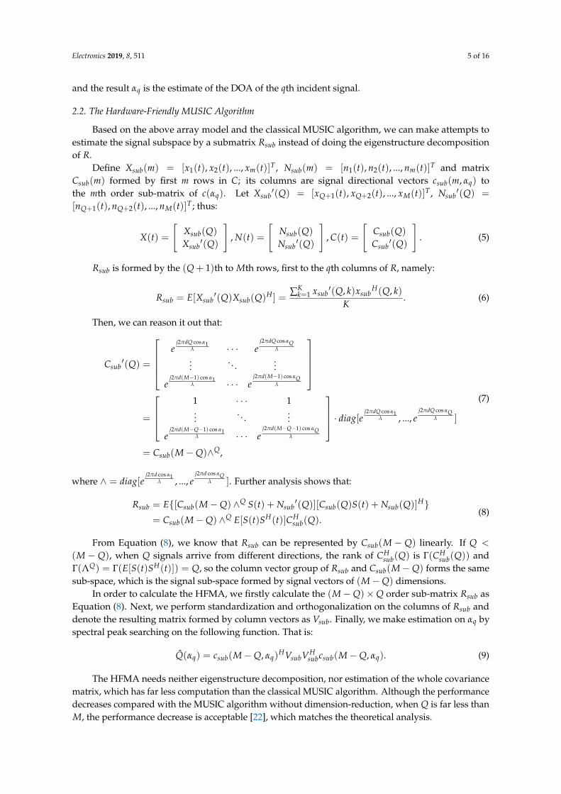
The accelerator can speed up the specific algorithms to implement the HFMA, which includesmatrix covariance, matrix multiply, matrix addition, direction vector computing (DVC), and spatialspectrum function calculating (SSFC). The detailed architecture of the accelerator is presented below.

From Figure 1, we know that the accelerator consists of a reconfigurable computation array (RCA),a reconfigurable controller (RC), a main controller (MC), a direct memory access (DMA) unit, an AXIinterface and an on-chip memory. The RCA has four reconfigurable processing elements (RPEs), and theyhave identical computational resources, which are listed in Figure 1. The RC manages the computationprocess and constructs the data paths between memory and RCA. The MC controls the acceleratorthat includes instruction decoding, DMA configuration, and RC configuration. The DMA and the AXIinterface are used to exchange data between off-chip and on-chip memory. The memory has a capacity of512 KB, and it is divided into 16 banks for high bandwidth and the parallelism requirement.

Figure 1. The architecture of the accelerator.

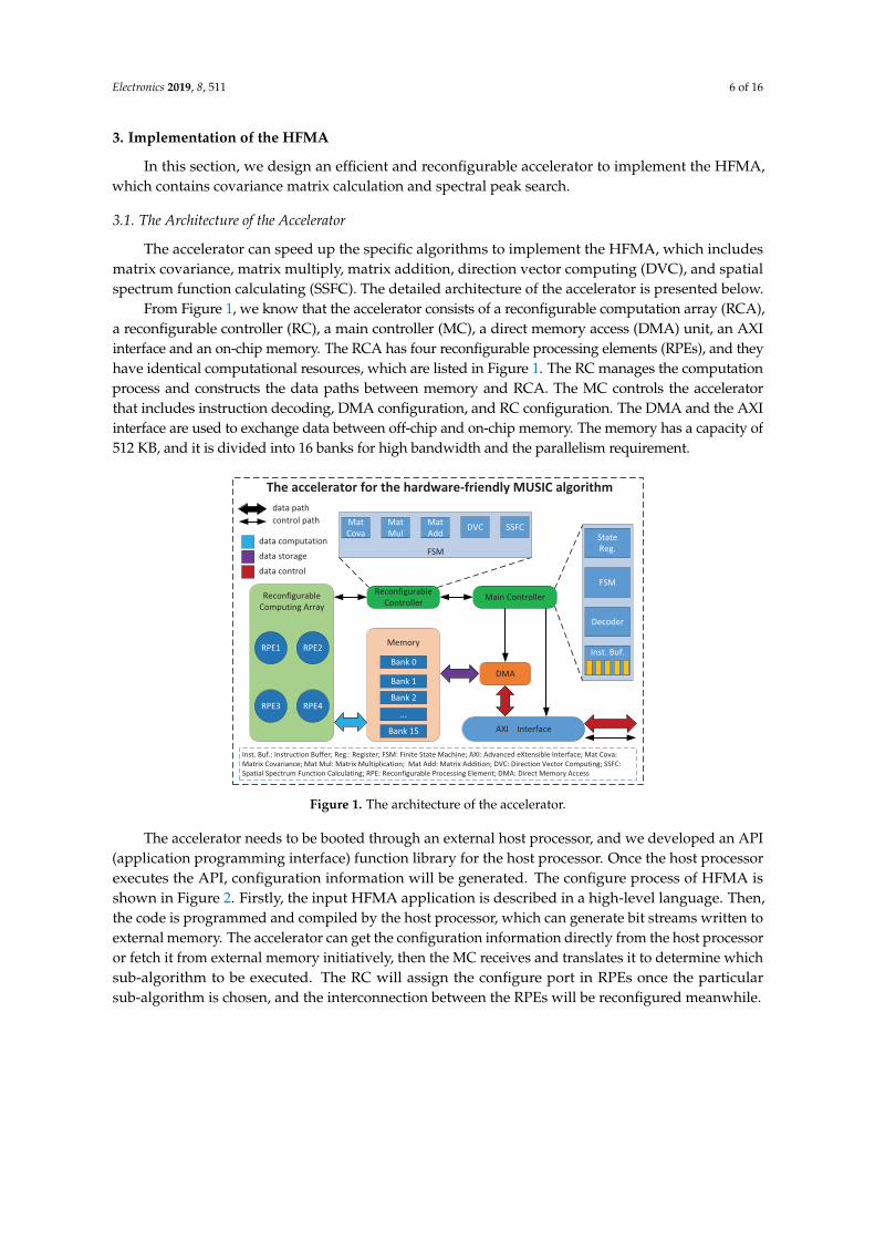
The accelerator needs to be booted through an external host processor, and we developed an API(application programming interface) function library for the host processor. Once the host processorexecutes the API, configuration information will be generated. The configure process of HFMA isshown in Figure 2. Firstly, the input HFMA application is described in a high-level language. Then,the code is programmed and compiled by the host processor, which can generate bit streams written toexternal memory. The accelerator can get the configuration information directly from the host processoror fetch it from external memory initiatively, then the MC receives and translates it to determine whichsub-algorithm to be executed. The RC will assign the configure port in RPEs once the particularsub-algorithm is chosen, and the interconnection between the RPEs will be reconfigured meanwhile.

Electronics 2019, 8, 511 7 of 16

Figure 2. The configuration process of the accelerator.

3.2. Implementation of Correlation Matrices’ Estimation

In this section, we propose an implementation method based on the partition to calculate thecovariance matrix, which is the first step of HFMA implementation. From Equation (6), it is obviousthat the estimate of the array covariance matrix is a calculation of matrix multiplication, but thecovariance matrix is a conjugate symmetric matrix in fact. Therefore, XXH can be converted to thefollowing formula:

XXH = Rnew(a, b) =

{X(a, :) · X∗(b, :), a ≥ b,

R∗new(a, b), a < b,(10)

where 1 ≤ a ≤ A, 1 ≤ b ≤ B, A is the row number, and B is the column number of the matrix to besolved. When a ≥ b, the lower triangular results of the covariance matrix can be obtained, while theupper triangular results are obtained by the conjugate symmetry property, which can greatly reducethe computation amount and improve the calculation speed.

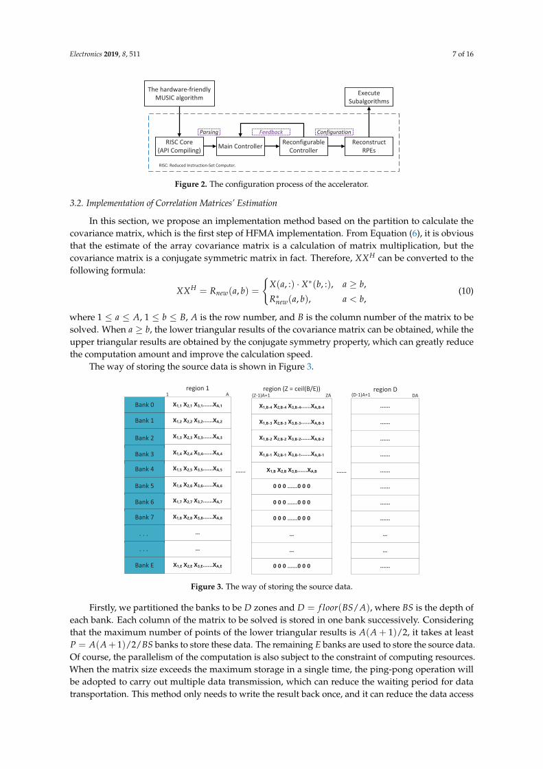
The way of storing the source data is shown in Figure 3.

Figure 3. The way of storing the source data.

Firstly, we partitioned the banks to be D zones and D = f loor(BS/A), where BS is the depth ofeach bank. Each column of the matrix to be solved is stored in one bank successively. Consideringthat the maximum number of points of the lower triangular results is A(A + 1)/2, it takes at leastP = A(A+ 1)/2/BS banks to store these data. The remaining E banks are used to store the source data.Of course, the parallelism of the computation is also subject to the constraint of computing resources.When the matrix size exceeds the maximum storage in a single time, the ping-pong operation willbe adopted to carry out multiple data transmission, which can reduce the waiting period for datatransportation. This method only needs to write the result back once, and it can reduce the data access

Electronics 2019, 8, 511 8 of 16

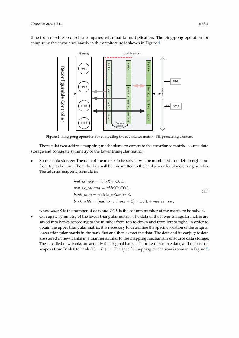
time from on-chip to off-chip compared with matrix multiplication. The ping-pong operation forcomputing the covariance matrix in this architecture is shown in Figure 4.

Figure 4. Ping-pong operation for computing the covariance matrix. PE, processing element.

There exist two address mapping mechanisms to compute the covariance matrix: source datastorage and conjugate symmetry of the lower triangular matrix.

• Source data storage: The data of the matrix to be solved will be numbered from left to right andfrom top to bottom. Then, the data will be transmitted to the banks in order of increasing number.The address mapping formula is:

matrix_row = addrX÷ COL,

matrix_column = addrX%COL,

bank_num = matrix_column%E,

bank_addr = (matrix_column÷ E)× COL + matrix_row,

(11)

where addrX is the number of data and COL is the column number of the matrix to be solved.• Conjugate symmetry of the lower triangular matrix: The data of the lower triangular matrix are

saved into banks according to the number from top to down and from left to right. In order toobtain the upper triangular matrix, it is necessary to determine the specific location of the originallower triangular matrix in the bank first and then extract the data. The data and its conjugate dataare stored in new banks in a manner similar to the mapping mechanism of source data storage.The so-called new banks are actually the original banks of storing the source data, and their reusescope is from Bank 0 to bank (15− P + 1). The specific mapping mechanism is shown in Figure 5.

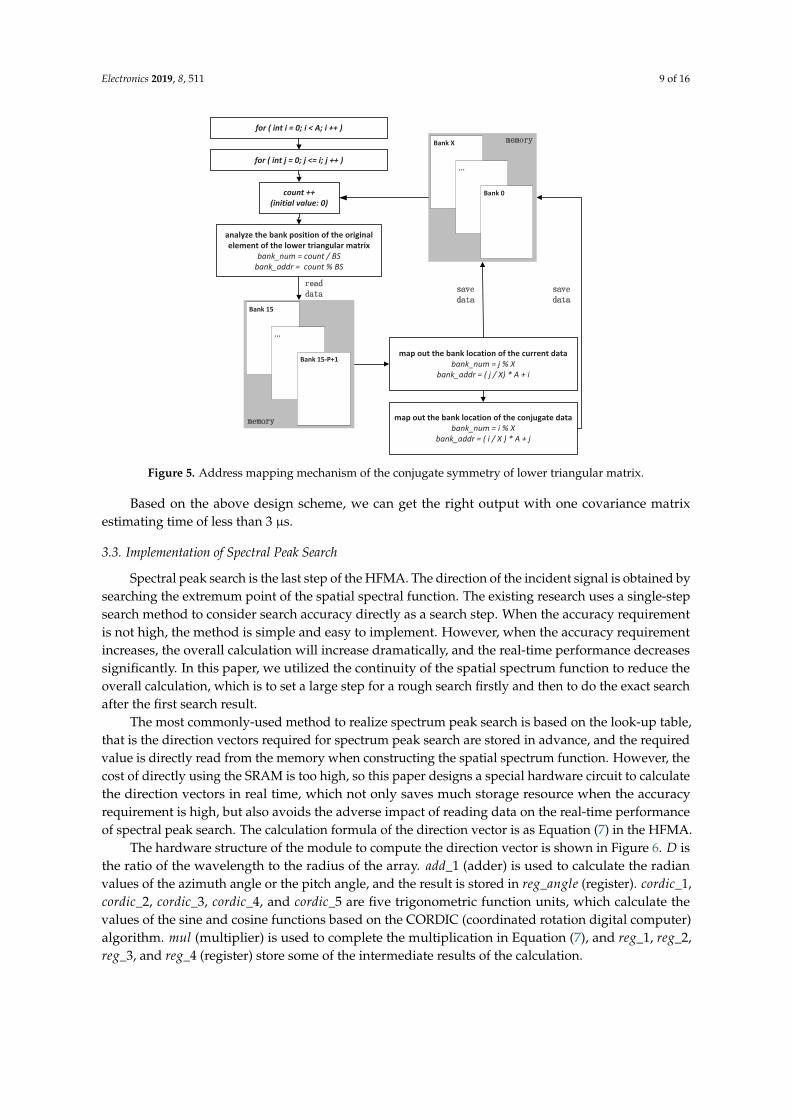
Electronics 2019, 8, 511 9 of 16

Figure 5. Address mapping mechanism of the conjugate symmetry of lower triangular matrix.

Based on the above design scheme, we can get the right output with one covariance matrixestimating time of less than 3 µs.

3.3. Implementation of Spectral Peak Search

Spectral peak search is the last step of the HFMA. The direction of the incident signal is obtained bysearching the extremum point of the spatial spectral function. The existing research uses a single-stepsearch method to consider search accuracy directly as a search step. When the accuracy requirementis not high, the method is simple and easy to implement. However, when the accuracy requirementincreases, the overall calculation will increase dramatically, and the real-time performance decreasessignificantly. In this paper, we utilized the continuity of the spatial spectrum function to reduce theoverall calculation, which is to set a large step for a rough search firstly and then to do the exact searchafter the first search result.

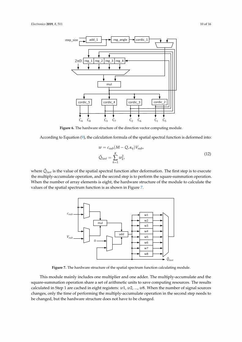
The most commonly-used method to realize spectrum peak search is based on the look-up table,that is the direction vectors required for spectrum peak search are stored in advance, and the requiredvalue is directly read from the memory when constructing the spatial spectrum function. However, thecost of directly using the SRAM is too high, so this paper designs a special hardware circuit to calculatethe direction vectors in real time, which not only saves much storage resource when the accuracyrequirement is high, but also avoids the adverse impact of reading data on the real-time performanceof spectral peak search. The calculation formula of the direction vector is as Equation (7) in the HFMA.

The hardware structure of the module to compute the direction vector is shown in Figure 6. D isthe ratio of the wavelength to the radius of the array. add_1 (adder) is used to calculate the radianvalues of the azimuth angle or the pitch angle, and the result is stored in reg_angle (register). cordic_1,cordic_2, cordic_3, cordic_4, and cordic_5 are five trigonometric function units, which calculate thevalues of the sine and cosine functions based on the CORDIC (coordinated rotation digital computer)algorithm. mul (multiplier) is used to complete the multiplication in Equation (7), and reg_1, reg_2,reg_3, and reg_4 (register) store some of the intermediate results of the calculation.

Electronics 2019, 8, 511 10 of 16

Figure 6. The hardware structure of the direction vector computing module.

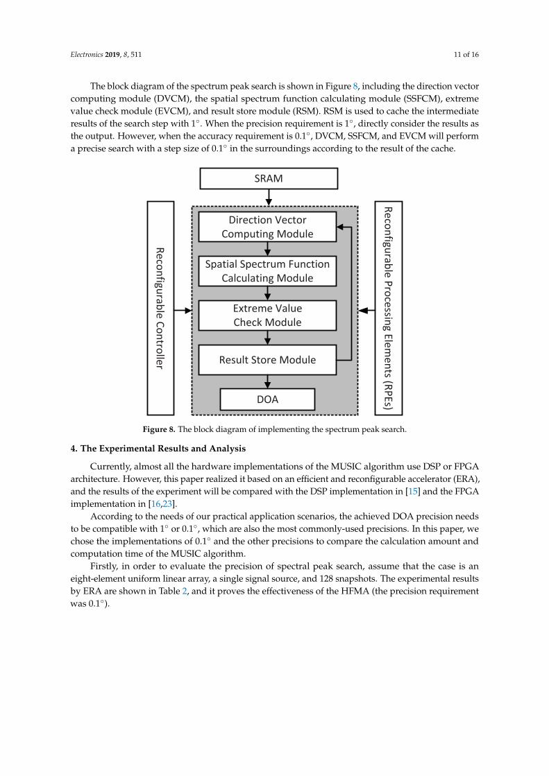
According to Equation (9), the calculation formula of the spatial spectral function is deformed into:

w = csub(M−Q, αq)Vsub,

Q̂last =K

∑k=1

w2k ,

(12)

where Q̂last is the value of the spatial spectral function after deformation. The first step is to executethe multiply-accumulate operation, and the second step is to perform the square-summation operation.When the number of array elements is eight, the hardware structure of the module to calculate thevalues of the spatial spectrum function is as shown in Figure 7.

Figure 7. The hardware structure of the spatial spectrum function calculating module.

This module mainly includes one multiplier and one adder. The multiply-accumulate and thesquare-summation operation share a set of arithmetic units to save computing resources. The resultscalculated in Step 1 are cached in eight registers: w1, w2, ..., w8. When the number of signal sourceschanges, only the time of performing the multiply-accumulate operation in the second step needs tobe changed, but the hardware structure does not have to be changed.

Electronics 2019, 8, 511 11 of 16

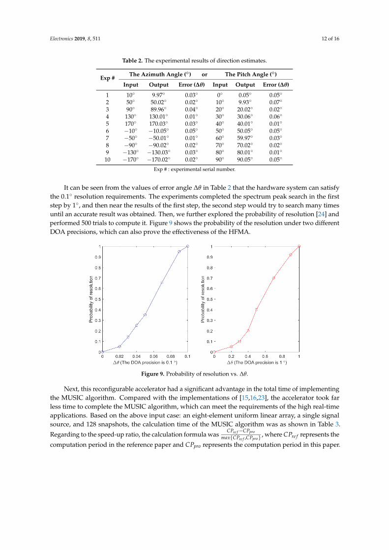
The block diagram of the spectrum peak search is shown in Figure 8, including the direction vectorcomputing module (DVCM), the spatial spectrum function calculating module (SSFCM), extremevalue check module (EVCM), and result store module (RSM). RSM is used to cache the intermediateresults of the search step with 1◦. When the precision requirement is 1◦, directly consider the results asthe output. However, when the accuracy requirement is 0.1◦, DVCM, SSFCM, and EVCM will performa precise search with a step size of 0.1◦ in the surroundings according to the result of the cache.

Figure 8. The block diagram of implementing the spectrum peak search.

4. The Experimental Results and Analysis

Currently, almost all the hardware implementations of the MUSIC algorithm use DSP or FPGAarchitecture. However, this paper realized it based on an efficient and reconfigurable accelerator (ERA),and the results of the experiment will be compared with the DSP implementation in [15] and the FPGAimplementation in [16,23].

According to the needs of our practical application scenarios, the achieved DOA precision needsto be compatible with 1◦ or 0.1◦, which are also the most commonly-used precisions. In this paper, wechose the implementations of 0.1◦ and the other precisions to compare the calculation amount andcomputation time of the MUSIC algorithm.

Firstly, in order to evaluate the precision of spectral peak search, assume that the case is aneight-element uniform linear array, a single signal source, and 128 snapshots. The experimental resultsby ERA are shown in Table 2, and it proves the effectiveness of the HFMA (the precision requirementwas 0.1◦).

Electronics 2019, 8, 511 12 of 16

Table 2. The experimental results of direction estimates.

Exp # The Azimuth Angle (◦) or The Pitch Angle (◦)

Input Output Error (∆θ) Input Output Error (∆θ)

1 10◦ 9.97◦ 0.03◦ 0◦ 0.05◦ 0.05◦

2 50◦ 50.02◦ 0.02◦ 10◦ 9.93◦ 0.07◦

3 90◦ 89.96◦ 0.04◦ 20◦ 20.02◦ 0.02◦

4 130◦ 130.01◦ 0.01◦ 30◦ 30.06◦ 0.06◦

5 170◦ 170.03◦ 0.03◦ 40◦ 40.01◦ 0.01◦

6 −10◦ −10.05◦ 0.05◦ 50◦ 50.05◦ 0.05◦

7 −50◦ −50.01◦ 0.01◦ 60◦ 59.97◦ 0.03◦

8 −90◦ −90.02◦ 0.02◦ 70◦ 70.02◦ 0.02◦

9 −130◦ −130.03◦ 0.03◦ 80◦ 80.01◦ 0.01◦

10 −170◦ −170.02◦ 0.02◦ 90◦ 90.05◦ 0.05◦

Exp # : experimental serial number.

It can be seen from the values of error angle ∆θ in Table 2 that the hardware system can satisfythe 0.1◦ resolution requirements. The experiments completed the spectrum peak search in the firststep by 1◦, and then near the results of the first step, the second step would try to search many timesuntil an accurate result was obtained. Then, we further explored the probability of resolution [24] andperformed 500 trials to compute it. Figure 9 shows the probability of the resolution under two differentDOA precisions, which can also prove the effectiveness of the HFMA.

Figure 9. Probability of resolution vs. ∆θ.

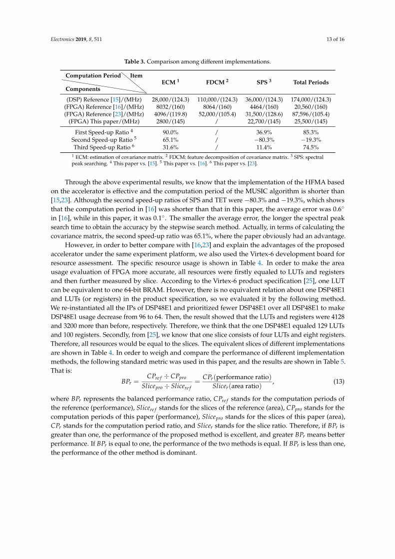
Next, this reconfigurable accelerator had a significant advantage in the total time of implementingthe MUSIC algorithm. Compared with the implementations of [15,16,23], the accelerator took farless time to complete the MUSIC algorithm, which can meet the requirements of the high real-timeapplications. Based on the above input case: an eight-element uniform linear array, a single signalsource, and 128 snapshots, the calculation time of the MUSIC algorithm was as shown in Table 3.

Regarding to the speed-up ratio, the calculation formula wasCPre f−CPpro

max{CPre f ,CPpro} , where CPre f represents the

computation period in the reference paper and CPpro represents the computation period in this paper.

Electronics 2019, 8, 511 13 of 16

Table 3. Comparison among different implementations.

Components

Computation Period ItemECM 1 FDCM 2 SPS 3 Total Periods

(DSP) Reference [15]/(MHz) 28,000/(124.3) 110,000/(124.3) 36,000/(124.3) 174,000/(124.3)(FPGA) Reference [16]/(MHz) 8032/(160) 8064/(160) 4464/(160) 20,560/(160)(FPGA) Reference [23]/(MHz) 4096/(119.8) 52,000/(105.4) 31,500/(128.6) 87,596/(105.4)

(FPGA) This paper/(MHz) 2800/(145) / 22,700/(145) 25,500/(145)

First Speed-up Ratio 4 90.0% / 36.9% 85.3%Second Speed-up Ratio 5 65.1% / −80.3% −19.3%Third Speed-up Ratio 6 31.6% / 11.4% 74.5%

1 ECM: estimation of covariance matrix. 2 FDCM: feature decomposition of covariance matrix. 3 SPS: spectralpeak searching. 4 This paper vs. [15]. 5 This paper vs. [16]. 6 This paper vs. [23].

Through the above experimental results, we know that the implementation of the HFMA basedon the accelerator is effective and the computation period of the MUSIC algorithm is shorter than[15,23]. Although the second speed-up ratios of SPS and TET were −80.3% and −19.3%, which showsthat the computation period in [16] was shorter than that in this paper, the average error was 0.6◦

in [16], while in this paper, it was 0.1◦. The smaller the average error, the longer the spectral peaksearch time to obtain the accuracy by the stepwise search method. Actually, in terms of calculating thecovariance matrix, the second speed-up ratio was 65.1%, where the paper obviously had an advantage.

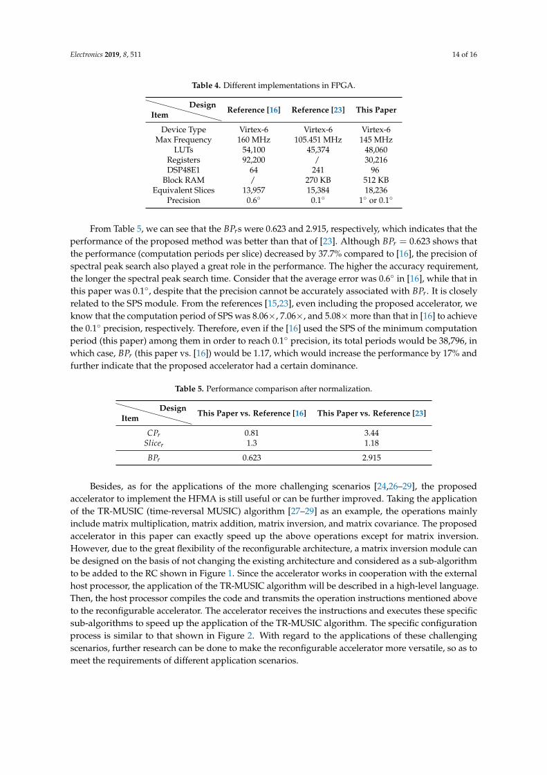
However, in order to better compare with [16,23] and explain the advantages of the proposedaccelerator under the same experiment platform, we also used the Virtex-6 development board forresource assessment. The specific resource usage is shown in Table 4. In order to make the areausage evaluation of FPGA more accurate, all resources were firstly equaled to LUTs and registersand then further measured by slice. According to the Virtex-6 product specification [25], one LUTcan be equivalent to one 64-bit BRAM. However, there is no equivalent relation about one DSP48E1and LUTs (or registers) in the product specification, so we evaluated it by the following method.We re-instantiated all the IPs of DSP48E1 and prioritized fewer DSP48E1 over all DSP48E1 to makeDSP48E1 usage decrease from 96 to 64. Then, the result showed that the LUTs and registers were 4128and 3200 more than before, respectively. Therefore, we think that the one DSP48E1 equaled 129 LUTsand 100 registers. Secondly, from [25], we know that one slice consists of four LUTs and eight registers.Therefore, all resources would be equal to the slices. The equivalent slices of different implementationsare shown in Table 4. In order to weigh and compare the performance of different implementationmethods, the following standard metric was used in this paper, and the results are shown in Table 5.That is:

BPr =CPre f ÷ CPpro

Slicepro ÷ Slicere f=

CPr(performance ratio)Slicer(area ratio)

, (13)

where BPr represents the balanced performance ratio, CPre f stands for the computation periods ofthe reference (performance), Slicere f stands for the slices of the reference (area), CPpro stands for thecomputation periods of this paper (performance), Slicepro stands for the slices of this paper (area),CPr stands for the computation period ratio, and Slicer stands for the slice ratio. Therefore, if BPr isgreater than one, the performance of the proposed method is excellent, and greater BPr means betterperformance. If BPr is equal to one, the performance of the two methods is equal. If BPr is less than one,the performance of the other method is dominant.

Electronics 2019, 8, 511 14 of 16

Table 4. Different implementations in FPGA.

ItemDesign Reference [16] Reference [23] This Paper

Device Type Virtex-6 Virtex-6 Virtex-6Max Frequency 160 MHz 105.451 MHz 145 MHz

LUTs 54,100 45,374 48,060Registers 92,200 / 30,216DSP48E1 64 241 96

Block RAM / 270 KB 512 KBEquivalent Slices 13,957 15,384 18,236

Precision 0.6◦ 0.1◦ 1◦ or 0.1◦

From Table 5, we can see that the BPrs were 0.623 and 2.915, respectively, which indicates that theperformance of the proposed method was better than that of [23]. Although BPr = 0.623 shows thatthe performance (computation periods per slice) decreased by 37.7% compared to [16], the precision ofspectral peak search also played a great role in the performance. The higher the accuracy requirement,the longer the spectral peak search time. Consider that the average error was 0.6◦ in [16], while that inthis paper was 0.1◦, despite that the precision cannot be accurately associated with BPr. It is closelyrelated to the SPS module. From the references [15,23], even including the proposed accelerator, weknow that the computation period of SPS was 8.06×, 7.06×, and 5.08×more than that in [16] to achievethe 0.1◦ precision, respectively. Therefore, even if the [16] used the SPS of the minimum computationperiod (this paper) among them in order to reach 0.1◦ precision, its total periods would be 38,796, inwhich case, BPr (this paper vs. [16]) would be 1.17, which would increase the performance by 17% andfurther indicate that the proposed accelerator had a certain dominance.

Table 5. Performance comparison after normalization.

ItemDesign This Paper vs. Reference [16] This Paper vs. Reference [23]

CPr 0.81 3.44Slicer 1.3 1.18

BPr 0.623 2.915

Besides, as for the applications of the more challenging scenarios [24,26–29], the proposedaccelerator to implement the HFMA is still useful or can be further improved. Taking the applicationof the TR-MUSIC (time-reversal MUSIC) algorithm [27–29] as an example, the operations mainlyinclude matrix multiplication, matrix addition, matrix inversion, and matrix covariance. The proposedaccelerator in this paper can exactly speed up the above operations except for matrix inversion.However, due to the great flexibility of the reconfigurable architecture, a matrix inversion module canbe designed on the basis of not changing the existing architecture and considered as a sub-algorithmto be added to the RC shown in Figure 1. Since the accelerator works in cooperation with the externalhost processor, the application of the TR-MUSIC algorithm will be described in a high-level language.Then, the host processor compiles the code and transmits the operation instructions mentioned aboveto the reconfigurable accelerator. The accelerator receives the instructions and executes these specificsub-algorithms to speed up the application of the TR-MUSIC algorithm. The specific configurationprocess is similar to that shown in Figure 2. With regard to the applications of these challengingscenarios, further research can be done to make the reconfigurable accelerator more versatile, so as tomeet the requirements of different application scenarios.

Electronics 2019, 8, 511 15 of 16

5. Conclusions

In this paper, the implementation of HFMA based on an efficient and reconfigurable architecturewas proposed. The implementation process was mainly divided into two steps: Firstly, we optimizedthe MUSIC algorithm to avoid the eigenvalue decomposition of the covariance matrix. Then, weimplemented the correlation matrices estimation and spectral peak search in the reconfigurablearchitecture. Our implementation can better speed up the MUSIC algorithm to meet the high real-timecapability for the DOA estimation and be compatible with both the 1◦ and 0.1◦ accuracy requirements.Synthesized under the TSMC 40-nm CMOS technology with the Synopsys Design Compiler, weobtained a maximum frequency of 1 GHz with a 4,765,475.4 µm2 area, and the power dissipation was238.27 mW. The experimental results showed that the total time of the MUSIC algorithm was 25.5 µs atthe frequency of 1 GHz, which was better than some previously-published work.

In the future, we will exploit the proposed architecture to estimate the number of sources, which isa necessary pre-requisite for spectral-based DOA methods. We envision that we can preset a thresholdvalue and compare the increasing range of all eigenvalues of the covariance matrix with it. If theincreasing range of two eigenvalues is less than the threshold, the eigenvalues are considered as noiseeigenvalues. When the increasing range of the two eigenvalues is greater than the threshold for the firsttime, it indicates that the two eigenvalues are the first signal eigenvalue and the last noise eigenvalue,so that the number of sources can be determined. Based on the above idea, we can further studywhether the proposed architecture can be used to optimize the algorithm after adding the thresholdvalue, so as to achieve the goal of reducing the computation amount. Besides, we can further studywhether the proposed HFMA is useful for other array structures.

Author Contributions: H.C. conceived of and designed the hardware-friendly algorithm and the accelerator; H.C.performed the experiments with support from K.C. (Kai Chen); H.C. analyzed the experimental results; H.C.,K.C. (Kaifeng Cheng), and Q.C. contributed to task decomposition and the corresponding implementations; H.C.wrote the paper; L.L. and Y.F. supervised the project.

Funding: This research received no external funding.

Acknowledgments: This research was supported by the National Nature Science Foundation of China underGrant No. 61176024; the project on the Integration of Industry, Education and Research of Jiangsu ProvinceBY2015069-05; the project Funded by the Priority Academic Program Development of Jiangsu Higher EducationInstitutions (PAPD); the Collaborative Innovation Center of Solid-State Lighting and Energy-Saving Electronics;Nanjing University Technology Innovation Fund No. 1480608201; and the Fundamental Research Funds for theCentral Universities.

Conflicts of Interest: The authors declare no conflict of interest.

References

1. Schmidt, R. Multiple Emitter Location and Signal Parameter Estimation. IEEE Trans. Antennas Propag. 1986,3, 276–280. [CrossRef]

2. Zoltowski, M.D.; Kautz, G.M.; Silverstein, S.D. Beamspace Root-MUSIC. IEEE Trans. Signal Process. 1993, 41, 344.[CrossRef]

3. Ren, Q.S.; Willis, A.J. Fast root MUSIC algorithm. Electron. Lett. 1997, 33, 450–451. [CrossRef]4. He, Z.S.; Li, Y.; Xiang, J.C. A modified root-music algorithm for signal DOA estimation. J. Syst. Eng. Electron.

1999, 10, 42–47.5. Cheng, Q.; Lei, H.; So, H.C. Improved Unitary Root-MUSIC for DOA Estimation Based on Pseudo-Noise

Resampling. IEEE Signal Process. Lett. 2014, 21, 140–144.6. Chen, Q.; Liu, R.L. On the explanation of spatial smoothing in MUSIC algorithm for coherent sources.

In Proceedings of the International Conference on Information Science and Technology, Nanjing, China,26–28 March 2011; pp. 699–702.

Electronics 2019, 8, 511 16 of 16

7. Iwai, T.; Hirose, N.; Kikuma, N.; Sakakibara, K.; Hirayama, H. DOA estimation by MUSIC algorithmusing forward-backward spatial smoothing with overlapped and augmented arrays. In Proceedings of theInternational Symposium on Antennas and Propagation Conference Proceedings, Kaohsiung, Taiwan, 2–5December 2014; pp. 375–376.

8. Wang, H.K.; Liao, G.S.; Xu, J.W.; Zhu, S.Q.; Zeng, C. Direction-of-Arrival Estimation for CirculatingSpace-Time Coding Arrays: From Beamspace MUSIC to Spatial Smoothing in the Transform Domain.Sensors 2018, 11, 3689. [CrossRef] [PubMed]

9. Zhao, Q.; Dong, M.; Liang, W.J. Research on modified MUSIC algorithm of DOA estimation. Comput. Eng.Appl. 2012, 48, 102–105.

10. Hong, W. An Improved Direction-finding Method of Modified MUSIC Algorithm. Shipboard Electron.Countermeas. 2011, 34, 71–73.

11. Wang, F.; Wang, J.Y.; Zhang, A.T.; Zhang, L.Y. The Implementation of High-speed parallel Algorithm ofReal-valued Symmetric Matrix Eigenvalue Decomposition through FPGA. J. Air Force Eng. Univ. 2008, 6,67–70.

12. Kim, Y.; Mahapatra, R.N. Dynamic Context Compression for Low-Power CoarseGrained ReconfigurableArchitecture. IEEE Trans. Very Large Scale Integr. (VLSI) Syst. 2010, 18, 15–28. [CrossRef]

13. Hwang, W.J.; Lee, W.H.; Lin, S.J.; Lai, S.Y. Efficient Architecture for Spike Sorting in Reconfigurable Hardware.Sensors 2013, 11, 14860–14887. [CrossRef] [PubMed]

14. Wang, S.J.; Liu, D.T.; Zhou, J.B.; Zhang, B.; Peng, Y. A Run-Time Dynamic Reconfigurable Computing Systemfor Lithium-Ion Battery Prognosis. Energies 2016, 8, 572. [CrossRef]

15. Li, M.; Zhao, Y.M. Realization of MUSIC Algorithm on TMS320C6711. Electron. Warf. Technol. 2005, 3, 36–38.16. Yan, J.; Huang, Y.Q.; Xu, H.T.; Vandenbosch, G.A.E. Hardware acceleration of MUSIC based DoA estimator

in MUBTS. In Proceedings of the 8th European Conference on Antennas and Propagation, The Hague,The Netherlands, 6–11 April 2014; pp. 2561–2565.

17. Sun, Y.; Zhang, D.L.; Li, P.P.; Jiao, R.; Zhang, B. The studies and FPGA implementation of spectrum peaksearch in MUSIC algorithm. In Proceedings of the International Conference on AntiCounterfeiting, Securityand Identification, Macao, China, 12–14 December 2014.

18. Deng, L.K.; Li, S.X.; Huang, P.K. Computation of the covariance matrix in MSNWF based on FPGA.Appl. Electron. Tech. 2007, 33, 39–42.

19. Wu, R.B. A novel universal preprocessing approach for high-resolution direction-of-arrival estimation.J. Electron. 1993, 3, 249–254.

20. TMS320C6672 Multicore Fixed and Floating-Point DSP (2014) Lit. no. SPRS708E; Texas Instruments Inc.: Dallas,TX, USA, 2014.

21. TMS320C66x DSP Library (2014) Lit. no. SPRC265; Texas Instruments Inc.: Dallas, TX, USA, 2014.22. Yu, J.Z.; Chen, D.C. A fast subspace algorithm for DOA estimation. Mod. Electron. Tech. 2005, 12, 90–92.23. Huang, K.; Sha, J.; Shi, W.; Wang, Z.F. An Efficient FPGA Implementation for 2-D MUSIC Algorithm.

Circuits Syst. Signal Process. 2016, 35, 1795–1805. [CrossRef]24. Wang, M.Z.; Nehorai, A. Coarrays, MUSIC, and the cramer–rao bound. IEEE Trans. Signal Process. 2017, 65,

933–946. [CrossRef]25. Virtex-6 Family Overview. Available online: http://www.xilinx.com/support/documentation/data_sheets/

ds150.pdf (accessed on 8 May 2019).26. Devaney, A.J. Time reversal imaging of obscured targets from multistatic data. IEEE Trans. Antennas Propag.

2005, 53, 1600–1610. [CrossRef]27. Ciuonzo, D.; Romano, G.; Solimene, R. On MSE performance of time-reversal MUSIC. In Proceedings of the

IEEE 8th Sensor Array and Multichannel Signal Processing Workshop (SAM), A Coruna, Spain, 22–25 June 2014.28. Ciuonzo, D.; Romano, G.; Solimene, R. Performance analysis of time-reversal MUSIC. IEEE Trans.

Signal Process. 2015, 63, 2650–2662. [CrossRef]29. Ciuonzo, D.; Rossi, P.S. Noncolocated time-reversal MUSIC: high-SNR distribution of null spectrum.

IEEE Signal Process. Lett. 2017, 24, 397–401. [CrossRef]

c© 2019 by the authors. Licensee MDPI, Basel, Switzerland. This article is an open accessarticle distributed under the terms and conditions of the Creative Commons Attribution(CC BY) license (http://creativecommons.org/licenses/by/4.0/).