Identifiersdoi 10.46298/jtcam.6737

Arxiv 2008.11494v3

HistoryReceived Aug 28, 2020Accepted Jan 18, 2021Published Jul 13, 2021

Associate EditorShaocheng Ji

ReviewersDazhi JiangNeil Ribe

Open Reviewdoi 10.5281/zenodo.5079356

LicenceCC BY 4.0

©The Authors

Journal of Theoretical,Computational andApplied Mechanicsov

erla

y

diamond open access

An effective parameterization of texture-inducedviscous anisotropy in orthotropic materials withapplication for modeling geodynamical flows

Javier Signorelli1, Riad Hassani2, Andréa Tommasi3, and Lucan Mameri3

1 Instituto de Física de Rosario, CONICET & Universidad Nacional de Rosario, Argentina2 Université Côte d’Azur, CNRS, Observatoire de la Côte d’Azur, IRD, Géoazur, France3 Géosciences Montpellier – CNRS & Université de Montpellier, France

We describe the mathematical formulation and the numerical implementation of an effective parame-terization of the viscous anisotropy of orthorhombic materials produced by crystallographic preferredorientations (CPO or texture), which can be integrated into 3D geodynamic and materials science codes.Here, the approach is applied to characterize the texture-induced viscous anisotropy of olivine polycrystals,the main constituent of the Earth’s upper mantle. The parameterization is based on the Hill (1948)orthotropic yield criterion. The coefficients of the Hill yield surface are calibrated based on numerical testsperformed using the second order Viscoplastic Self-consistent (SO-VPSC) model. The parameterization wasimplemented in a 3D thermo-mechanical finite-element code developed to model large-scale geodynamicalflows, in the form of a Maxwell rheology combining isotropic elastic and anisotropic non-linear viscousbehaviors. The implementation was validated by comparison with results of the analytical solution and ofthe SO-VPSC model for simple shear and axial compression of a homogeneous anisotropic material. Anapplication designed to examine the effect of texture-induced viscous anisotropy on the reactivation ofmantle shear zones in continental plates highlights unexpected couplings between localized deformationcontrolled by variations in the orientation and intensity of the olivine texture in the mantle and themechanical behavior of the elasto-viscoplastic overlying crust. Importantly, the computational time onlyincreases by a factor 2-3 with respect to the classic isotropic Maxwell viscoelastic rheology.

Keywords: creep, viscous anisotropy, texture, second-order VPSC, geodynamics, olivine

1 IntroductionThe greatest challenge in modeling the dynamics of the solid Earth is to reproduce the extremelyheterogeneous deformation of the outer layer of the planet – the tectonic plates, which havethicknesses ranging from a few km at oceanic ridges to > 200 km beneath some continentaldomains, in response to the continuous motion that animates the underlying convective mantle.An additional challenge is to simulate the repeated reactivation of some plate boundaries withintervals of hundreds of million years, (e.g., Wilson 1966; Vauchez et al. 1997). This behaviorimplies long-time preservation of rheological heterogeneity produced by deformation in responseto episodes of collision or breakup of tectonic plates. Two processes have been proposedas the causes for this behavior: (1) grain size reduction (Bercovici and Ricard 2014) and (2)viscous anisotropy (Tommasi and Vauchez 2001; Tommasi et al. 2009). Here, we focus on thesecond process. All major rock-forming minerals have low symmetries (hexagonal, trigonal,orthorhombic, monoclinic, or triclinic) and, by consequence, strongly anisotropic thermo-mechanical behaviors. In addition, tectonic plates deform mostly by non-linear viscoplasticprocesses, mainly dislocation creep. Deformation produces therefore strong preferred orientationsof the crystals that compose the rocks (texture), which transfer part of the intrinsic anisotropy ofthe physical properties of the rock-forming minerals to larger scales (texture-induced anisotropy).

Olivine, which is the major constituent (60 − 80 %) of the, in most cases, strongest section of

Journal of Theoretical, Computational and Applied Mechanics July 2021

jtcam.episciences.org 1 17

Signorelli et al. An effective parameterization of texture-induced viscous anisotropy in orthotropic materials

the tectonic plates (50 − 90 % of the total thickness of the plate), is orthorhombic. It displays amarked anisotropy of its thermal and mechanical properties (Tommasi et al. 2001; Abramson et al.1997; Bai et al. 1991). Geodynamical flows produce olivine textures, which are only significantlymodified (strengthened or weakened and have their orientation and symmetry changed) byfurther deformation, (e.g., Nicolas and Christensen 1987; Wenk et al. 1991; Tommasi et al.2000). Seismological measurements are able to detect the elastic anisotropy produced by thesetextures, (e.g., Hess 1964; Savage 1999; Tommasi and Vauchez 2015). These data record patternsof active or old (fossilized) olivine textures, which are homogeneous at the scale of severaltens to hundreds of km in the upper mantle. These textures produce viscoplastic anisotropy atlarge-scale (Knoll et al. 2009; Hansen et al. 2012; Mameri et al. 2019), which in turn modifiessubsequent deformation. Texture-induced viscous anisotropy has been proposed as a majorfeature of plate tectonics, explaining the reactivation of ancient structures, even at hundreds ofmillion years of interval (Vauchez et al. 1997; Tommasi and Vauchez 2001; Tommasi et al. 2009). Ithas also been proposed to modify the convective patterns and the interactions between theplates and the convective mantle (Castelnau et al. 2009; Lev and Hager 2011; Blackman et al.2017). A precise description of the viscous anisotropy produced by olivine textures was achievedby explicitly coupling viscoplastic self-consistent calculations of polycrystal deformation intogeodynamical flow models (Knoll et al. 2009; Tommasi et al. 2009; Castelnau et al. 2009; Blackmanet al. 2017). However, this approach remains too time and memory-consuming for widespread use.

Hierarchical multi-scale modelling provides a path for exchanging information betweensystems with different characteristic length scales. Several strategies may be defined (Gawad et al.2015; Jiang 2014). In the present work, we adopt the virtual-experiment strategy for exploringthe viscosity tensor of a textured material composed of orthorhombic crystals, using crystalplasticity modeling (i.e. a micromechanical crystal plasticity model captures texture-inducedevolution of plastic anisotropy). Since simulations are able to calculate the material response atany point of the yield surface, the virtual-experiment strategy provides a method for identifyingthe parameters in the yield function for deformation modes. This strategy allows combining theaccuracy of the description of the texture-induced viscous anisotropy of the polycrystal modeland the numerical performance of the yield functions (Plunkett et al. 2006).

In this article, we describe the mathematical formulation and the numerical implementationof a parameterization of the anisotropic viscoplastic rheology of olivine polycrystals in a 3Dfinite-element thermo-mechanical code (Adeli3D, Hassani et al. 1997). The parameterization isbased on the Hill (1948) orthotropic yield criterion in which the coefficients that calibrated theHill yield surface are based on numerical tests performed using the second order ViscoplasticSelf-Consistent (SO-VPSC) model. The aim is to provide a simplified Maxwell rheology model,combining isotropic elastic and anisotropic non-linear viscous behavior, that can be integratedinto 3D geodynamic and materials science codes, allowing the physical description of a complexmulti-scale system with reasonable computational times.

2 Parameterizing texture-induced viscous anisotropy in viscoelasticorthotropic materialsThe framework presented in this section to parameterize the anisotropic rheology of an olivinepolycrystal is based on the notion of hierarchical multi-scale modelling. It extends the classicalviscoelastic Maxwell model to consider viscous anisotropy calibrated based on the Hill (1948)orthotropic yield criterion. The parameters describing the anisotropy at the coarse-scale (platetectonics) are identified using fine-scale (rock sample) virtual experiments performed usingviscoplastic self-consistent simulations of the deformation of an olivine polycrystal.

2.1 Thermo-mechanical codeWe implemented the viscous anisotropy parameterization in the 3D thermo-mechanical codeAdeli3D (Hassani et al. 1997), which is optimized to model large-scale geodynamical flows,focusing on the deformation of the lithosphere, i.e. the semi-rigid plates that compose theouter layer of the Earth. The code is based on a Lagrangian finite-element discretization ofthe quasi-static mechanical behavior of the lithosphere, which solves the obtained non-linear

Journal of Theoretical, Computational and Applied Mechanics July 2021

jtcam.episciences.org 2 17

Signorelli et al. An effective parameterization of texture-induced viscous anisotropy in orthotropic materials

equations using a dynamic relaxation method (Cundall 1988). The problem consists in finding thevelocity field v and the symmetric tensor 𝝈 satisfying

div𝝈 + 𝜌ℓg = 0𝐷𝝈

𝐷𝑡= M(𝝈 ,D), 𝑖𝑛 Ω (1)

in the physical domain Ω, where g is the acceleration vector due to gravity, 𝜌ℓ is the lithospheredensity and 2D = ∇v + ∇v⊤, 𝐷

𝐷𝑡is an objective time derivative associated with the large strain

formulation (Malvern 1969). Jaumann and Green-Naghdi are the most frequently used objectivederivatives (see, for example, (Johnson and Bammann 1984)). They can be expressed using thesame formulation:

𝐷𝝈

𝐷𝑡= ¤𝝈 − W𝝈 + 𝝈W, (2)

with W = 𝝎, for the Jaumann derivative and W = Ω, for the Green-Naghdi derivative, where

𝜔𝑖 𝑗 =12

( 𝜕𝑉𝑖𝜕𝑥 𝑗

− 𝜕𝑉𝑗

𝜕𝑥𝑖

)(3)

is the material spin tensor, i.e. the screw part of the velocity gradient 𝜕𝑉𝑖𝜕𝑥 𝑗

, and Ω = ¤RR⊤, therotation rate associated with the left polar decomposition of the deformation gradient F (F = RU,where R is an orthogonal tensor and U is a symmetric tensor called right stretch tensor). Asgenerally done, we use the Jaumann corotational stress rate in our simulations.

The functional M in Equation (1) stands for a general hypoelastic1 constitutive law. Inthe present case, M describes a Maxwell rheology combining isotropic elastic and anisotropicnon-linear viscous behavior. The transition between the elastic and viscous regimes depends onthe temperature and stress, which change the viscosity, and on the considered time-scale.

2.2 Maxwell viscoelasticityThe viscoelastic constitutive law combines the contributions of the elastic De and the viscous Dvstrain-rates. The total strain-rate is defined as D = De + Dv and the constitutive relationship isgiven by

𝐷𝝈

𝐷𝑡= 2` (D − Dv) + _ tr(D − Dv)I (4)

with I, the second-order identity tensor, tr, the trace operator, and ` and _, the Lamé moduli. Theviscous strain-rate Dv is given by the flow rule

Dv =𝜕Φ

𝜕𝝈(5)

where Φ(𝝈) is a viscous potential. A typical choice for this potential is the power-law equation

Φ(𝝈) = 23

𝛾

𝑛 + 1 𝐽 (𝝈)𝑛+1 (6)

where 𝐽 (𝝈) is the equivalent stress, defined based on Von Mises yield function.2 In the isotropiccase, 𝛾 = 𝛾0 exp(−𝑄/𝑅𝑇 ), where 𝑛,𝑄 and 𝛾0 are the experimentally-derived power-law exponent,activation energy in J mol−1 K−1, and fluidity3 in Pa−n s−1, respectively; 𝑅 is the gas constant

1 In hypoelastic constitutive models, the objective stress rate is related to the rate of deformation through an elasticitytensor.

2 The Von Mises yield function defines a five-dimensional (for an incompressible material) surface in the six-dimensionalspace of stress: 2𝐽 2 (𝝈) = (𝜎11 − 𝜎22)2 + (𝜎22 − 𝜎33)2 + (𝜎33 − 𝜎11)2 + 6(𝜎212 + 𝜎223 + 𝜎231), 𝐽 (𝝈) > 0. When the stressstate lies on this surface the material is said to have reached the yield condition.

3 The fluidity is a material parameter, which depends on the physico-chemical conditions of the deformation, relatingthe deviatoric stress to the strain-rate.

Journal of Theoretical, Computational and Applied Mechanics July 2021

jtcam.episciences.org 3 17

Signorelli et al. An effective parameterization of texture-induced viscous anisotropy in orthotropic materials

and 𝑇 , the temperature in Kelvin. Using Equation (5) and Equation (6), the viscous part of thetotal strain-rate can be expressed as

Dv =23𝛾 𝐽 (𝝈)

𝑛 𝜕𝐽 (𝝈)𝜕𝝈

. (7)

To describe an anisotropic viscous behavior, the yield condition is here defined based on theorthotropic yield function of Hill (1948).

2.2.1 Hill (1948) orthotropic yield criterionThe Hill yield function, which builds on the Von Mises’ concept of plastic potential, definesa pressure-independent homogeneous quadratic criterion. It assumes that the reference axesare the principal axes of anisotropy of the material, which are orthogonal. The resulting yieldfunction takes the form

𝐽 (𝝈) = (𝐹 (𝜎11 − 𝜎22)2 +𝐺 (𝜎22 − 𝜎33)2 + 𝐻 (𝜎33 − 𝜎11)2 + 2𝐿𝜎212 + 2𝑀𝜎223 + 2𝑁𝜎231

)1/2. (8)

To predict the viscous contribution of anisotropic materials under multiaxial stress conditions,𝐽 (𝝈) is considered as the definition of the equivalent stress and Equation (7) becomes

Dv = 𝛾 𝐽 (𝝈)𝑛−1A : S (9)

where S is the deviatoric part of 𝝈 and A is a rank-4 tensor describing the material anisotropy, andthe stress dependency of 𝐽 is omitted in order to simplify the notation. Using the Voigt notation,A has the following matrix representation in the reference frame defined by the principal axes ofanisotropy of the material:

A =23

𝐹 + 𝐻 −𝐹 −𝐻 0 0 0−𝐹 𝐺 + 𝐹 −𝐺 0 0 0−𝐻 −𝐺 𝐻 +𝐺 0 0 00 0 0 𝐿 0 00 0 0 0 𝑀 00 0 0 0 0 𝑁

, (10)

where 𝐹 , 𝐺 , 𝐻 , 𝐿,𝑀 , and 𝑁 are the Hill yield surface coefficients, which describe the anisotropyof the material. In the case of an isotropic aggregate, 𝐹 = 𝐺 = 𝐻 = 1/2 and 𝐿 = 𝑀 = 𝑁 = 3/2,and Equation (8) reduces to the Von Mises yield function. With this particular choice of thepotential, the viscous strain-rate is traceless and the Maxwell constitutive law takes the form

𝐷𝝈

𝐷𝑡= 2`D + _ tr(D)I − 2`𝛾 𝐽𝑛−1A : S. (11)

2.2.2 Numerical integrationIt is convenient to split the constitutive law given in Equation (4) in deviatoric and hydrostaticparts that can be integrated separately:

¤S + j𝝎 (S) = 2` (D′ − D′v) (12a)

¤𝑝 = 𝐾 tr(D) (12b)

where D′ and D′v (= Dv) are the deviatoric parts of the total and viscous strain-rate tensors,

respectively, 𝑝 is the mean pressure, and j𝝎 (S) = S𝛚 + (S𝛚)⊤ when the Jaumann derivative isused; ` and 𝐾 are the shear and bulk moduli of the material, respectively.

Assuming D and 𝛚 are constant in the time interval [𝑡, 𝑡 + Δ𝑡] and using the Crank-Nicolsonscheme, the stress at time station 𝑡 + Δ𝑡 is sought as the solution of the non-linear equation:

S𝑡+Δ𝑡 = S𝑡 + 2`Δ𝑡D′ − `Δ𝑡D′v(S𝑡 ) −

Δ𝑡

2 j𝝎 (S𝑡 ) − `Δ𝑡D′v(S𝑡+Δ𝑡 ) −

Δ𝑡

2 j𝝎 (S𝑡+Δ𝑡 ), (13a)

𝑝𝑡+Δ𝑡 = 𝑝𝑡 + 𝐾 tr(D). (13b)

Journal of Theoretical, Computational and Applied Mechanics July 2021

jtcam.episciences.org 4 17

Signorelli et al. An effective parameterization of texture-induced viscous anisotropy in orthotropic materials

Equation (13a) can be expressed as r(S𝑡+Δ𝑡 ) = 0, with

r(S) = S + `Δ𝑡D′v(S) +

Δ𝑡

2 j𝝎 (S) − S (14)

where S groups together the terms known at the beginning of the time interval (𝑡 ):

S = S𝑡 + 2`Δ𝑡D′ − `Δ𝑡D′v(S𝑡 ) −

Δ𝑡

2 j𝝎 (S𝑡 ) . (15)

Defining R as the coordinate system fixed to the laboratory frame and R, the corresponding axesfixed related to the material anisotropy (material coordinate system) in this case, a second-ordertensor X defined in R can be expressed in R through a rotation matrix 𝑅0, which allows changingfrom the material to laboratory reference frame (i.e., from R to R):

X = R⊤0 XR0. (16)

Expressing Equation (14) and Equation (15) in the material reference frame R, we obtain

r(S) = S + `Δ𝑡D′v(S) +

Δ𝑡

2 j (S) − ˆS (17)

ˆS = S𝑡 + 2`Δ𝑡D′ − `Δ𝑡D′

v(S𝑡 ) − Δ𝑡

2 j𝝎 (S𝑡 ) (18)

where S = R⊤0 SR0 and D′ = R⊤

0 D′R0. Newton’s method is used to solve the non-linear systemr(S) = 0 and the inverse rotation is applied to find the deviatoric stress at 𝑡 + Δ𝑡 in the laboratoryreference frame.

The numerical implementation in Adeli3D (hereinafter referred as Adeli3D-anis) of theprocedure described in this section allows a parameterized description of the viscous anisotropycomponent of any orthotropic viscoelastic material. The implementation was validated bycomparing numerical and semi-analytical solutions for simple settings (see Appendix A).

2.3 Determining the Hill coefficients for olivine polycrystals using the VPSC modelThe constitutive relationship presented above includes the effects of anisotropy through theHill coefficients. In Materials Sciences, these coefficients are determined through a set ofmechanical tests. However, such tests are unfeasible for geological materials because viscousdeformation is only attained experimentally at high confining pressures, limiting the possiblegeometry of laboratory experiments. Thus, we calibrate the Hill coefficients, which describe thetexture-induced viscous anisotropy of olivine polycrystals, based on VPSC polycrystal plasticitysimulations.

Unlike the upper and lower bound models, the VPSC formulation allows each grain to deformaccording to its orientation and the strength of the interaction with its surroundings. Each grainis considered as an ellipsoidal inclusion surrounded by a homogeneous effective medium thathas the average properties of the polycrystal. Several choices are possible for the linearizedbehavior at grain level. The secant (Hill 1965; Hutchinson 1976), affine (Ponte Castañeda 1996;Masson et al. 2000), and tangent approaches (Molinari et al. 1987; Lebensohn and Tomé 1993) arefirst-order approximations, which disregard higher-order statistical information inside the grains.However, for highly anisotropic materials displaying a strong contrast in mechanical behaviorbetween differently oriented grains, such as olivine, the second order approximation (SO-VPSC),which takes into account average field fluctuations inside the grains (Ponte Castañeda 2002), is abetter choice (Castelnau et al. 2008). For completeness, a brief description of the theoreticalframework of SO-VPSC is presented below. The viscoplastic constitutive behavior is described bythe rate-sensitive relation

d(x) =∑𝑠

m𝑠 (x) ¤𝛾𝑠 (x) = ¤𝛾𝑜∑𝑠

m𝑠 (x)m𝑠 (x) : s(x)

𝝉𝑠𝑐 (x)𝑛 sign(m𝑠 (x) : s(x)), (19)

where 2m𝑠 = n𝑠 ⊗ b𝑠 + b𝑠 ⊗ n𝑠 is defined as a symmetric tensor, with n𝑠 and b𝑠 the normalsto the slip systems’ glide plane and the Burgers’ vector, respectively. Quantity ¤𝛾𝑠 represents

Journal of Theoretical, Computational and Applied Mechanics July 2021

jtcam.episciences.org 5 17

Signorelli et al. An effective parameterization of texture-induced viscous anisotropy in orthotropic materials

the strain-rate accommodated by the slip system 𝑠 , and ¤𝛾𝑜 is a normalization factor. The stressexponent 𝑛 is the rate-sensitivity exponent and 𝜏𝑠𝑐 is the critical resolved shear stress of theslip system 𝑠 . The tensors d and s are the local strain-rate and deviatoric stress, respectively.Linearizing Equation (19), we obtain

d(x) = l : s(x) + d0 (20a)D = L : S + D0 (20b)

where l and L are the viscoplastic compliances, d0 and D0 are the back-extrapolated terms at thelevel of the grain and of the aggregate, respectively, and D and S are the macroscopic deviatoricstrain-rate and stress tensors.

The effective stress potential of the polycrystal described by Equation (20b) may be written inthe form

𝑈𝑇 =12L :: (S ⊗ S) + D0 : S + 1

2𝐺 (21)

which expresses the effective potential𝑈𝑇 of the nonlinear viscoplastic polycrystal in terms of alinearly viscous aggregate with properties determined from variational principles. The last term𝐺/2 in Equation (21) is the energy under zero applied stress. The average second-order momentof the stress field is the fourth-order tensor

⟨s ⊗ s⟩ = 2𝑐

𝜕𝑈𝑇𝜕l

=1𝑐

𝜕L𝜕l

:: (S ⊗ S) + 1𝑐

𝜕D0

𝜕l: S + 1

𝑐

𝜕𝐺

𝜕l(22)

where 𝑐 is the volume fraction of a given grain. From the average second-order moments of thestress, the associated second-order of the strain-rate can then be evaluated as

⟨d ⊗ d⟩ = (l ⊗ l) :: ⟨s ⊗ s⟩ + d ⊗ d0 + d0 ⊗ d − d0 ⊗ d0. (23)

The average second-order moments of the stress field over each grain are obtained by calcu-lating the derivatives in Equation (22). The implementation of the second-order procedure inVPSC follows the work of Liu and Ponte Castañeda (2004). For more details, see the VPSC7cmanual (Tomé and Lebensohn 2012).

2.3.1 Polycrystal Equipotential SurfaceThe anisotropy of a viscoplastic material can be described by comparing points that belong tothe same reference equipotential surface. This requires probing the material in a given stressdirection, while ensuring that the associated dissipation rate will be the same regardless ofthe chosen direction. This reference Polycrystal Equipotential Surface (PES) is the locus of allstress states associated with a polycrystal with a given texture. In the present study, we use theSO-VPSC polycrystal plasticity model to estimate the PES.

The plastic potential is essentially a function of the stress that can be differentiated to derivethe plastic strain-rate. This function 𝑓 (S) is defined by a constant plastic work rate, ¤𝑊0, along thepotential. The plastic work rate for an arbitrary macroscopic strain-rate, D0, is defined as

𝑓 (S) = S : D = S0 : D0 = ¤𝑊0 (24)

where S0 is the stress state corresponding to a given D0 (or inversely). This function defines aseries of convex surfaces in the deviatoric stress space, which are equipotential surfaces when𝑓 (S) is constant. As S or D is not known a priori, the obtained plastic potential rate can bedifferent from ¤𝑊0. In this case, the stress point does not lie on the selected equipotential. Thestress or strain-rate on the selected equipotential can be obtained based on Hutchinson (1976),which showed that when the magnitude of the strain-rate is changed by a factor Z , the stressresponse of the polycrystal becomes

S(ZD) = Z𝑛S(D) . (25)

As a consequence, the magnitude of S or D can be scaled as follows: D∗ = D( ¤𝑊0/ ¤𝑊 )𝑛/(1+𝑛) andS∗ = S( ¤𝑊0/ ¤𝑊 )1/(1+𝑛) . The standard VPSC code imposes the strain-rate vectors D and calculates

Journal of Theoretical, Computational and Applied Mechanics July 2021

jtcam.episciences.org 6 17

Signorelli et al. An effective parameterization of texture-induced viscous anisotropy in orthotropic materials

the associated stress S for probing the material response. As mentioned above, both tensors canbe renormalized to give the same dissipation rate for every point of the yield surface. The testdirection in the strain-rate space is given by 𝑛𝑖 𝑗 = 𝐷𝑖 𝑗/∥D∥, where ∥D∥ = √

𝐷𝑖 𝑗𝐷𝑖 𝑗 defines thelength of the strain-rate tensor D. Thus, the strain-rate tensor can be characterized by a polarrepresentation, which consists of a radius in strain-rate (deviatoric stress) space, ∥D∥, and a set ofdirection cosines (𝑛𝑖 𝑗 ). In this representation ∥D∥ is an independent variable, whereas the ninevalues of 𝑛𝑖 𝑗 are not. Since D is a symmetric deviatoric second-order tensor, it is possible torepresent the strain-rate tensor by a five-component unit vector using a second-order tensor withan orthonormal symmetric base 𝑛𝑖 𝑗 = 𝑛_𝑏_𝑖 𝑗 , _ = 1, . . . , 5 (see Appendix B). Using generalizedspherical coordinates, the vector n can be expressed as

𝑛 (1) = cos\1 sin\2 sin\3 sin\4 sin\5, 𝑛 (2) = cos\2 sin\3 sin\4 sin\5,𝑛 (3) = cos\3 sin\4 sin\5, 𝑛 (4) = cos\4 sin\5,𝑛 (5) = cos\5

(26)

with −𝜋 ≤ \ ≤ 𝜋 or 0 ≤ \ ≤ 𝜋/2 for centro or non-centro symmetric evaluation, respectively.As an example, if simulations are restricted to the 𝑆1 − 𝑆2 subspace, thus, \1 = 0,−𝜋 ≤ \2 ≤ 𝜋 ,\3 = \4 = \5 = 𝜋/2, and Equation (26) reduces to 𝑛 (1) = sin\2, 𝑛 (2) = cos\2 𝑛 (3) = 0, 𝑛 (4) = 0,and 𝑛 (5) = 0 with \2 scanned in steps of 15° and the probed strain-rate (deviatoric stress) tensorset to ∥D∥ = 1. Here, we extend the original implementation of the PES calculation in the VPSCcode (Tomé and Lebensohn (2012) – VPSC7c manual) by allowing to choose whether the samplingpoints will be equispaced in strain-rate or in stress.

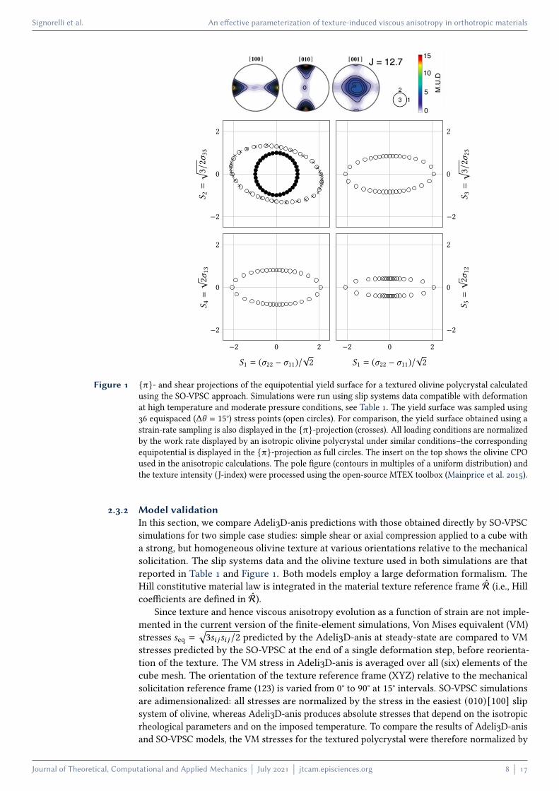
As an example, we present in Figure 1 the π- and shear projections of the PES for an olivineaggregate with a typical orthorhombic texture, described by 1000 orientations. The orientationdistribution function (ODF) and texture intensity (J-index) were quantified using the open-sourceMTEX toolbox (Mainprice et al. 2015). The olivine slip systems data in Table 1 are derived fromexperiments at high temperature and moderate pressure conditions (Bai et al. 1991).

Table 1 Slip systems parameters used in the SO-VPSCsimulations. aAdimensional values; normalizedby flow stress of the (010) [100] slip system;bSlip systems not active in olivine, used forstabilizing the calculations, but accommodating≪ 5 % strain in all simulations.

Slip Systems Critical ResolvedShear Stressa

StressExponent

(010) [100] 1 3(001) [100] 1 3(010) [001] 2 3(100) [001] 3 3(011) [100] 4 3(110) [001] 6 3111⟨110⟩b 50 3111⟨011⟩b 50 3111⟨101⟩b 50 3

All curves are normalized by the work rate of an isotropic olivine polycrystal deformedunder similar conditions (full symbols). No appreciable differences are obtained using eitherstrain-rate or stress sampling for the calculation of the yield surfaces. Since only intracrystallineglide deformation modes are taken into account (no twinning), the predicted surfaces arecentro-symmetric. The four equipotential surfaces are then fitted using a least-square method toobtain the six coefficients (𝐹 , 𝐺 , 𝐻 , 𝐿,𝑀 , 𝑁 ) that satisfy the anisotropic Hill yield function (seeEquation (9)). Table 2 presents the fitted coefficients for the orthorhombic texture shown inFigure 1.

Sampling variable 𝐹 𝐺 𝐻 𝐿 𝑀 𝑁

Strain-rate (err = 0.034) 0.0220 0.2208 0.3769 8.6133 2.0777 2.3101Stress (err = 0.028) 0.0225 0.2275 0.3744 8.9183 2.1258 2.3016

Table 2 Hill coefficients obtained by imposing either strain-rate or stress for sampling the PES

Journal of Theoretical, Computational and Applied Mechanics July 2021

jtcam.episciences.org 7 17

Signorelli et al. An effective parameterization of texture-induced viscous anisotropy in orthotropic materials

−2

0

2

S 2=√ 3/

2σ33

−2

0

2

S 3=√ 3/

2σ23

−2 0 2

−2

0

2

S1 = (σ22 − σ11)/√2

S 4=√ 2σ

13

−2 0 2

−2

0

2

S1 = (σ22 − σ11)/√2

S 5=√ 2σ

12

Figure 1 π- and shear projections of the equipotential yield surface for a textured olivine polycrystal calculatedusing the SO-VPSC approach. Simulations were run using slip systems data compatible with deformationat high temperature and moderate pressure conditions, see Table 1. The yield surface was sampled using36 equispaced (Δ\ = 15°) stress points (open circles). For comparison, the yield surface obtained using astrain-rate sampling is also displayed in the π-projection (crosses). All loading conditions are normalizedby the work rate displayed by an isotropic olivine polycrystal under similar conditions–the correspondingequipotential is displayed in the π-projection as full circles. The insert on the top shows the olivine CPOused in the anisotropic calculations. The pole figure (contours in multiples of a uniform distribution) andthe texture intensity (J-index) were processed using the open-source MTEX toolbox (Mainprice et al. 2015).

2.3.2 Model validationIn this section, we compare Adeli3D-anis predictions with those obtained directly by SO-VPSCsimulations for two simple case studies: simple shear or axial compression applied to a cube witha strong, but homogeneous olivine texture at various orientations relative to the mechanicalsolicitation. The slip systems data and the olivine texture used in both simulations are thatreported in Table 1 and Figure 1. Both models employ a large deformation formalism. TheHill constitutive material law is integrated in the material texture reference frame R (i.e., Hillcoefficients are defined in R).

Since texture and hence viscous anisotropy evolution as a function of strain are not imple-mented in the current version of the finite-element simulations, Von Mises equivalent (VM)stresses 𝑠eq =

√3𝑠𝑖 𝑗𝑠𝑖 𝑗/2 predicted by the Adeli3D-anis at steady-state are compared to VM

stresses predicted by the SO-VPSC at the end of a single deformation step, before reorienta-tion of the texture. The VM stress in Adeli3D-anis is averaged over all (six) elements of thecube mesh. The orientation of the texture reference frame (XYZ) relative to the mechanicalsolicitation reference frame (123) is varied from 0° to 90° at 15° intervals. SO-VPSC simulationsare adimensionalized: all stresses are normalized by the stress in the easiest (010) [100] slipsystem of olivine, whereas Adeli3D-anis produces absolute stresses that depend on the isotropicrheological parameters and on the imposed temperature. To compare the results of Adeli3D-anisand SO-VPSC models, the VM stresses for the textured polycrystal were therefore normalized by

Journal of Theoretical, Computational and Applied Mechanics July 2021

jtcam.episciences.org 8 17

Signorelli et al. An effective parameterization of texture-induced viscous anisotropy in orthotropic materials

the VM of an olivine polycrystal with 1000 randomly oriented grains, which has an isotropicmechanical response.

Two sets of boundary conditions were considered in the axial extension tests. For the first

BC1 BC2 BC3

1 m1 m

free slip free face fixed face

1

2

3

(a)

[100] [010] [001]

𝑍

𝑋 𝑌 Numerical modelsAdeli3D-anisSO-VPSC

0 15 30 45 60 75 900

0.5

1

1.5

2

2.5

3

BC1

BC2

(b)

Angle (°) between 𝑋𝑌 plane and extension

Normalized

vonMise

sequ

ivalentstre

ss

𝑋

𝑍𝑌0°

𝑋 𝑍𝑌

45°

𝑋

𝑍

𝑌90°

0 15 30 45 60 75 90

BC3(c)

Angle (°) between 𝑋𝑌 plane and simple shear plane

𝑋 𝑍𝑌

45°

𝑋

𝑍𝑌

90°𝑋

𝑍

𝑌

0°

Figure 2 (a) Imposed boundary conditions in Adeli3D-anis simulations and velocity gradient tensors (L) imposed inthe corresponding SO-VPSC simulations: Lext extension and Lss simple shear. BC: boundary conditions.Comparison of the predictions of anisotropic ADELI3D and SO-VPSC simulations: (b) axial extensionaltests with two sets of boundary conditions (BC1 = two planes of symmetry and BC2 = a single planeof symmetry); (c) simple shear test (BC3). Parameters describing the isotropic and anisotropic part ofthe rheology in the Adeli3D-anis simulations are presented in Table 3 and Table 2 (stress sampling),respectively.

set (BC1 in Figure 2(a)), extension was imposed in the Adeli3D-anis simulation by applying aconstant velocity normal to the face normal to axis 2 of the cube and keeping the opposite facefixed, one of the faces normal to axes 1 and 3 is a symmetry plane (free slip conditions) and theother is free (free face). This correspond to mixed boundary conditions in SO-VPSC simulations,where an extensional velocity 22 is imposed, all shear velocity components are imposed null(𝐿𝑖≠𝑗 = 0), and equal non-null stresses 11 and 33 are imposed. The corresponding tensor reads:

L1−ext =∗ 0 00 0.8 00 0 ∗

(27)

where the symbol * indicates that the magnitude of the component is unknown and mustbe determined as a computational result. In the second set of boundary conditions (BC2 inFigure 2(a)), the two faces normal to axis 1 are free in the Adeli3D-anis simulations. Thiscorresponds to SO-VPSC simulations where the extensional velocity 22, a null velocity to half of

Journal of Theoretical, Computational and Applied Mechanics July 2021

jtcam.episciences.org 9 17

Signorelli et al. An effective parameterization of texture-induced viscous anisotropy in orthotropic materials

the shear components (𝐿12 = 𝐿13 = 𝐿23 = 0), equal non null stresses 11 and 33, and null shearstresses. The predicted solutions for all loading-geometries are remarkably similar between theAdeli3D-anis and the SO-VPSC models for the two sets of boundary conditions, Figure 2(b). Thecorresponding tensor reads:

L2−ext =∗ ∗ ∗0 0.8 ∗0 0 ∗

. (28)

The less stringent boundary conditions (BC2), i.e. allowing a rigid rotation, results in lowernormalized VM stresses for all solicitations oblique to the texture reference frame, except at 45°,see Figure 2(b). In our case, due to the symmetry of the initial olivine texture, this rigid rotationmay only occur around the extension axis.

Simple shear tests were performed by applying a constant tangential velocity parallel toaxis 1 on the face normal to axis 2, keeping the opposite face fixed, and imposing null normalvelocities to the two faces normal to axis 3 (BC3 in Figure 2(a)). The corresponding tensor reads:

LSS =

0 1.4 00 0 00 0 0

. (29)

Equivalent boundary conditions are simulated in SO-VPSC by imposing a non-null component 12and null values to all other components of the velocity gradient tensor. The stress variation as afunction of the orientation of the imposed shear relative to the texture reference frame predictedby Adeli3D-anis and SO-VPSC models are also remarkably similar (Figure 2(c)), confirming thatthe present parameterization based on the Hill (1948) yield function is suitable for describing theviscous anisotropy of an olivine polycrystal with an orthotropic texture.

𝐸 (GPa) a 𝑛 𝛾0 (Pa−n s−1) 𝑄 (kJ/mol) 𝑇 (K)100 0.25 3 10−18 500 1423

Table 3 Parameters describing the isotropic part of the rheology in the validation tests.

3 Application: effect of texture-induced viscous anisotropy associatedwith fossil shear zones on the deformation of a continental plateViscoplastic deformation of mantle rocks in lithospheric-scale shear zones, i.e., narrow zonesaccommodating shear displacements between relatively undeformed domains of a tectonicplate, leads to development of olivine textures that may be preserved for very long time spans(hundreds of millions years, cf. (Tommasi and Vauchez 2015)). Anisotropic viscosity due to fossilolivine texture in mantle shear zones has been argued to trigger localized deformation in theplates when the mechanical solicitation is oblique to the trend of the shear zones, leading tothe formation of new plate boundaries parallel to these ancient structures (Vauchez et al. 1997;Tommasi and Vauchez 2001; Tommasi et al. 2009). However, previous simulations testing theseeffects, which directly coupled VPSC polycrystal plasticity models into the finite-element codessimulating the geodynamical flows, were too computationally demanding for full investigation ofthe interactions between texture-induced anisotropy and other strain localization processes activeon Earth. The parameterization presented here allows for a significant gain in both computationtime and memory requirements, enabling to run 3D geodynamical models that explicitly considerthe effect of texture-induced viscous anisotropy in the mantle on the plates’ dynamics. Its firstapplication in geodynamics (Mameri et al. 2020) focused on investigating the possible role oftexture-induced viscous anisotropy in the mantle in producing enigmatic alignments of activeseismicity in intraplate settings. This work testifies that texture-induced viscous anisotropy inthe mantle may produce strain localization not only in the mantle, but also in the overlyingcrust (Figure 3). A detailed analysis of the geological aspects of the problem are presentedin (Mameri et al. 2020), but these simulations allowed to investigate the feedbacks between

Journal of Theoretical, Computational and Applied Mechanics July 2021

jtcam.episciences.org 10 17

Signorelli et al. An effective parameterization of texture-induced viscous anisotropy in orthotropic materials

localized deformation controlled by texture-induced viscous anisotropy in the mantle and thedeformation processes in the brittle (plastic) upper crust. Parameters controlling the isotropicpart of the mantle and crust rheologies are shown in Table 4.

30 35 40 45 50 55 60 65 70 75 80 85 9010−1

100

101

102

Adeli3D-anisTime ≈ 2 My

Angle (°) between fossil mantle shear zone and compression

Strain

localization 30 35 40 45 50 55 60 65 70 75 80 85 90

0102030405060708090100

SO-VPSC Olivine Slip Systems

Angle (°) between [100]-max and compression

Activ

ity(%)

[001] (010)[100] (001)[100] (010)

Figure 3 Strain localization quantified as the ratio between the average of second-invariant of the strain-rate withinthe fossil mantle shear zone and outside it for different orientations of the fossil shear zone relatively tothe imposed shortening. The model represents a 1100 km long, 500 km wide, and 120 km thick continentalplate containing a fossil shear zone marked by a change in viscous anisotropy simulating a change withthe olivine texture in the lithospheric mantle. The Hill parameters in the fossil shear zone are coherent anolivine texture formed in response to a past strike-slip deformation (horizontal shear in a vertical plane).The surrounding mantle has Hill parameters simulating a random texture. Strain localizes in the fossilshear zone when it is oblique to the imposed compression, but strain localization is not symmetrical withrespect to the orientation of the fossil shear zone relative to the imposed compression. These predictionsreflect correctly the contrast in CRSS between the different slip systems in olivine, see Table 1, andtheir relative activity as predicted by SO-VPSC simulations considering a polycrystal with the texture(orientation and intensity) used to define the viscous anisotropy in the fossil shear zone for each model(insert). Maximum strain localization occurs when the fossil shear zone is at 45° to the compression, whereshear stresses resolved onto the easy [100] (010) slip system in most olivine crystals are maximum. Thelower strain localization in simulations with the fossil shear zone at 60° to the compression relative to thatin simulations with the fossil shear zone at 30° to the compression is consistent with the higher activity ofthe hard [001] (010) slip system in the former.

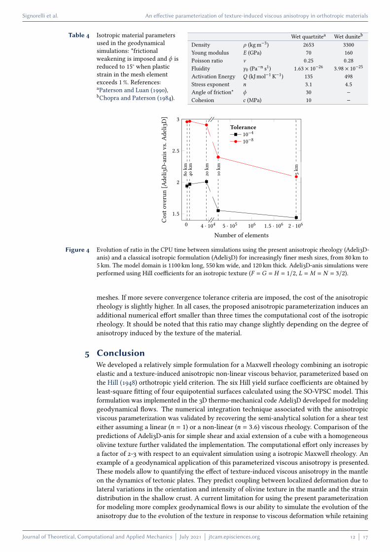
4 Computational costFigure 4 compares the cost associated with using the present anisotropic Maxwell rheologyrelatively to the classical isotropic formulation for simulations with increasing number ofelements. Plane strain compression is imposed to a plate with either a homogeneous isotropicrheology (Adeli3D) or Hill parameters simulating a random texture (Adeli3D-anis). Parameterscontrolling the isotropic part of the rheology are the same in the two simulations (Table 4). Twodifferent tolerance values for convergence in the flow law integration were tested. Both isotropicand anisotropic computation times increase almost linearly with the number of elements. Thus,the ratio between the CPU time for the isotropic and the anisotropic simulations does not dependsignificantly on the mesh size. It even decreases with increasing mesh size, stabilizing for fine

Journal of Theoretical, Computational and Applied Mechanics July 2021

jtcam.episciences.org 11 17

Signorelli et al. An effective parameterization of texture-induced viscous anisotropy in orthotropic materials

Table 4 Isotropic material parametersused in the geodynamicalsimulations: *frictionalweakening is imposed and 𝜙 isreduced to 15° when plasticstrain in the mesh elementexceeds 1 %. References:aPaterson and Luan (1990),bChopra and Paterson (1984).

Wet quartzitea Wet duniteb

Density 𝜌 (kgm−3) 2653 3300Young modulus 𝐸 (GPa) 70 160Poisson ratio a 0.25 0.28Fluidity 𝛾0 (Pa−n s1) 1.63 × 10−26 3.98 × 10−25Activation Energy 𝑄 (kJmol−1 K−1) 135 498Stress exponent 𝑛 3.1 4.5Angle of friction* 𝜙 30 −Cohesion 𝑐 (MPa) 10 −

0 4 · 104 5 · 105 106 1.5 · 106 2 · 1061.5

2

2.5

3

80km

40km

20km

10km

5km

Tolerance10−410−8

Number of elements

Costoverun

[Adeli3D-anisv

s.Ad

eli3D]

Figure 4 Evolution of ratio in the CPU time between simulations using the present anisotropic rheology (Adeli3D-anis) and a classical isotropic formulation (Adeli3D) for increasingly finer mesh sizes, from 80 km to5 km. The model domain is 1100 km long, 550 km wide, and 120 km thick. Adeli3D-anis simulations wereperformed using Hill coefficients for an isotropic texture (𝐹 = 𝐺 = 𝐻 = 1/2, 𝐿 = 𝑀 = 𝑁 = 3/2).

meshes. If more severe convergence tolerance criteria are imposed, the cost of the anisotropicrheology is slightly higher. In all cases, the proposed anisotropic parameterization induces anadditional numerical effort smaller than three times the computational cost of the isotropicrheology. It should be noted that this ratio may change slightly depending on the degree ofanisotropy induced by the texture of the material.

5 ConclusionWe developed a relatively simple formulation for a Maxwell rheology combining an isotropicelastic and a texture-induced anisotropic non-linear viscous behavior, parameterized based onthe Hill (1948) orthotropic yield criterion. The six Hill yield surface coefficients are obtained byleast-square fitting of four equipotential surfaces calculated using the SO-VPSC model. Thisformulation was implemented in the 3D thermo-mechanical code Adeli3D developed for modelinggeodynamical flows. The numerical integration technique associated with the anisotropicviscous parameterization was validated by recovering the semi-analytical solution for a shear testeither assuming a linear (𝑛 = 1) or a non-linear (𝑛 = 3.6) viscous rheology. Comparison of thepredictions of Adeli3D-anis for simple shear and axial extension of a cube with a homogeneousolivine texture further validated the implementation. The computational effort only increases bya factor of 2-3 with respect to an equivalent simulation using a isotropic Maxwell rheology. Anexample of a geodynamical application of this parameterized viscous anisotropy is presented.These models allow to quantifying the effect of texture-induced viscous anisotropy in the mantleon the dynamics of tectonic plates. They predict coupling between localized deformation due tolateral variations in the orientation and intensity of olivine texture in the mantle and the straindistribution in the shallow crust. A current limitation for using the present parameterizationfor modeling more complex geodynamical flows is our ability to simulate the evolution of theanisotropy due to the evolution of the texture in response to viscous deformation while retaining

Journal of Theoretical, Computational and Applied Mechanics July 2021

jtcam.episciences.org 12 17

Signorelli et al. An effective parameterization of texture-induced viscous anisotropy in orthotropic materials

the computational efficiency. This is part of an ongoing study, where different strategies areevaluated.

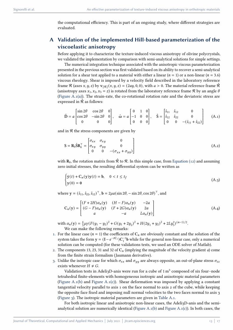
A Validation of the implemented Hill-based parameterization of theviscoelastic anisotropyBefore applying it to characterize the texture-induced viscous anisotropy of olivine polycrystals,we validated the implementation by comparison with semi-analytical solutions for simple settings.

The numerical integration technique associated with the anisotropic viscous parameterizationpresented in the previous section was first validated based on its ability to recover a semi-analyticalsolution for a shear test applied to a material with either a linear (𝑛 = 1) or a non-linear (𝑛 = 3.6)viscous rheology. Shear is imposed by a velocity field described in the laboratory referenceframe R (axes 𝑥,𝑦, 𝑧) by v[R] (𝑥,𝑦, 𝑧) = (2𝑎𝑦, 0, 0), with 𝑎 > 0. The material reference frame R(anisotropy axes 𝑥1, 𝑥2, 𝑥3 = 𝑧) is rotated from the laboratory reference frame R by an angle \(Figure A.1(a)). The strain-rate, the co-rotational rotation rate and the deviatoric stress areexpressed in R as follows:

D = 𝑎

sin 2\ cos 2\ 0cos 2\ −sin 2\ 0

0 0 0

, = 𝑎

0 1 0−1 0 00 0 0

, S =

𝑠11 𝑠12 0𝑠12 𝑠22 00 0 −(𝑠11 + 𝑠22)

(A.1)

and in R the stress components are given by

S = R0SR⊤0 =

𝜎𝑥𝑥 𝜎𝑥𝑦 0𝜎𝑥𝑦 𝜎𝑦𝑦 00 0 −(𝜎𝑥𝑥 + 𝜎𝑦𝑦)

(A.2)

with R0, the rotation matrix from R to R. In this simple case, from Equation (12) and assumingzero initial stresses, the resulting differential system can be written as

¤y(𝑡) + C𝑛 (y)y(𝑡) = b, 0 < 𝑡 ≤ 𝑡𝑓y(0) = 0

(A.3)

where y = (𝑠11, 𝑠22, 𝑠12)⊤, b = 2`𝑎(sin 2\,− sin 2\, cos 2\ )⊤, and

C𝑛 (y) =(𝐹 + 2𝐻 )𝛼𝑛 (y) (𝐻 − 𝐹 )𝛼𝑛 (y) −2𝑎(𝐺 − 𝐹 )𝛼𝑛 (y) (𝐹 + 2𝐺)𝛼𝑛 (y) 2𝑎

𝑎 −𝑎 𝐿𝛼𝑛 (y)

(A.4)

with 𝛼𝑛 (y) = 43`𝛾 (𝐹 (𝑦1 − 𝑦2)2 +𝐺 (𝑦1 + 2𝑦2)2 + 𝐻 (2𝑦1 + 𝑦2)2 + 2𝐿𝑦23) (𝑛−1)/2.

We can make the following remarks:1. For the linear case (𝑛 = 1) the coefficients of C𝑛 are obviously constant and the solution of the

system takes the form y = (I−𝑒−𝑡C1)C−11 b while for the general non-linear case, only a numerical

solution can be computed (for these validations tests, we used an ODE solver of Matlab).2. The components 13, 23, 31 and 32 of C𝑛 (implying the magnitude of the velocity gradient a) come

from the finite strain formalism (Jaumann derivative).3. Unlike the isotropic case for which 𝜎𝑥𝑥 and 𝜎𝑦𝑦 are always opposite, an out-of-plane stress 𝜎𝑧𝑧

exists whenever 𝐻 ≠ 𝐺 .Validation tests in Adeli3D-anis were run for a cube of 1m3 composed of six four–node

tetrahedral finite-elements with homogeneous isotropic and anisotropic material parameters(Figure A.1(b) and Figure A.1(c)). Shear deformation was imposed by applying a constanttangential velocity parallel to axis 1 on the face normal to axis 2 of the cube, while keepingthe opposite face fixed and imposing null normal velocities to the two faces normal to axis 3(Figure 3). The isotropic material parameters are given in Table A.1.

For both isotropic linear and anisotropic non-linear cases, the Adeli3D-anis and the semi-analytical solution are numerically identical (Figure A.1(b) and Figure A.1(c)). In both cases, the

Journal of Theoretical, Computational and Applied Mechanics July 2021

jtcam.episciences.org 13 17

Signorelli et al. An effective parameterization of texture-induced viscous anisotropy in orthotropic materials

_ (GPa) ` (GPa) 𝑛 𝛾0 (Pa−n s−1) 𝑄 (kJmol−1) 𝑇 (K)Test 1 40 40 1 0.5 × 10−12 500 1423Test 2 40 40 3.6 0.5 × 10−18 500 1423

Table A.1 Parameters describing the isotropic part of the rheology in the validation tests.

R𝑥

𝑦

1

O

𝑥1R

𝑥2

\

v = (2𝑎, 0, 0)(a)

Solution:Adeli3D-anis(Semi)-Analytical

•

0 20 40 60−10

−5

0

5

10

15σxy

σxx

σzz = 0

σyy

(b)

Time (s)

σ(M

Pa)

0 5000 10000 15000 20000−400

−200

0

200

400

600σxy

σxx

σzz

σyy

(c)

Figure A.1 (a) Simple shear tests for validating the implementation of the parameterization of the viscous anisotropyin large deformations for the general case of a misalignment \ = 30° between the anisotropy axes (R)with respect to the laboratory axes (R). Components of the stress tensor as a function of time for thesemi-analytical solution and the Hill-based parameterization of the viscoplastic anisotropy implementedin Adeli3D-anis: (b) Newtonian isotropic case (von Mises: 𝐹 = 0.5, 𝐿 = 1.5, 𝐺 = 0.5, 𝑀 = 1.5, 𝐻 = 0.5,𝑁 = 1.5) with 𝑛 = 1 and 𝑎 = 10−2 s−1; (c) non-Newtonian anisotropic case (Hill: 𝐹 = 0.0, 𝐿 = 8.9, 𝐺 = 0.2,𝑀 = 2.1, 𝐻 = 0.3, 𝑁 = 2.2) with 𝑛 = 3.6, 𝑎 = 10−6 s−1, and \ = 30°. The Hill yield surface coefficients aredefined in the material texture reference frame R, which is orthotropic. They correspond to those of anisotropic and a strongly textured olivine polycrystal, determined following the approach described inSection 2.3. Shear is imposed parallel to the maximum concentration of [100] of the texture. The factor 𝑎is proportional to the norm of the imposed velocity gradient.

imposed simple shear deformation is associated with a dominant 𝜎𝑥𝑦 stress component, butthe presence of a texture-induced anisotropy results in enhancement of this shear componentrelatively to the diagonal ones. As it is mentioned above anisotropy (𝐻 ≠ 𝐺) induces a 3D stressfield, where an out-of-plane stress 𝜎𝑧𝑧 takes place (Figure A.1(c)).

B Orthonormal base for second- and fourth-order symmetric tensorsWhen dealing with incompressible media, it is convenient to explicitly decompose stress andstrain-rate into deviatoric and hydrostatic components and to confine them to different subspaces,which may be decoupled for certain mechanical regimes. There are different ways of achievingsuch a decomposition. In the present calculations, we express the second-order tensorial quantitiesin an orthonormal basis of second-order symmetric tensors b_ , defined as

b1 =1√2

−1 0 00 1 00 0 0

, b2 =

1√6

−1 0 00 −1 00 0 2

, b3 =

1√2

0 0 00 0 10 1 0

, (B.1)

Journal of Theoretical, Computational and Applied Mechanics July 2021

jtcam.episciences.org 14 17

Signorelli et al. An effective parameterization of texture-induced viscous anisotropy in orthotropic materials

and

b4 =1√2

0 0 10 0 01 0 0

, b5 =

1√2

0 1 01 0 00 0 0

, b6 =

1√3

1 0 00 1 00 0 1

. (B.2)

The components of this basis have the property 𝑏_𝑖 𝑗𝑏_

′𝑖 𝑗= 𝛿__′ and provide a unique ‘vector’ and

‘matrix’ representation of second- and fourth-order symmetric tensors, respectively. In theparticular case of the stress tensor 𝜎𝑖 𝑗 = 𝜎_𝑏_𝑖 𝑗 where 𝜎_ = 𝜎𝑖 𝑗𝑏

_𝑖 𝑗. The orthonormality of the basis

guarantees that the six-dimensional strain-rate and stress vectors are work conjugates, i.e.

𝑑_𝜎_ = 𝑑𝑖 𝑗𝜎𝑖 𝑗 . (B.3)

The explicit form of the six components (𝜎1, 𝜎2, 𝜎3, 𝜎4, 𝜎5, 𝜎6) of 𝜎_ is(𝜎22 − 𝜎11√2

,2𝜎33 − 𝜎11 − 𝜎22√

6,√2𝜎23,

√2𝜎13,

√2𝜎12,

𝜎11 + 𝜎22 + 𝜎33√3

)(B.4)

and similarly for the components 𝑑_ . It is clear that in this representation the first five componentsare deviatoric and the sixth is proportional to the hydrostatic component of the tensor. conversely,to convert back the vector to the second-order tensor

𝜎11 𝜎12 𝜎13

𝜎22 𝜎23sym 𝜎33

=

− 𝜎1√

2 −𝜎2√6 +

𝜎6√3

𝜎5√2

𝜎4√2

𝜎1√2 −

𝜎2√6 +

𝜎6√3

𝜎3√2

sym 2𝜎2√6 + 𝜎6√

3

. (B.5)

ReferencesAbramson, E. H., J. M. Brown, L. J. Slutsky, and J. Zaug (1997). The elastic constants of San Carlos

olivine to 17 GPa. Journal of Geophysical Research: Solid Earth 102(B6):12253–12263. [doi].Bai, Q., S. J. Mackwell, and D. L. Kohlstedt (1991). High-temperature creep of olivine single

crystals 1. Mechanical results for buffered samples. Journal of Geophysical Research 96(B2):2441.[doi], [oa].

Bercovici, D. and Y. Ricard (2014). Plate tectonics, damage and inheritance. Nature 508(7497):513–516. [doi].

Blackman, D., D. Boyce, O. Castelnau, P. Dawson, and G. Laske (2017). Effects of crystal preferredorientation on upper-mantle flow near plate boundaries: rheologic feedbacks and seismicanisotropy. Geophysical Journal International 210(3):1481–1493. [doi], [hal].

Castelnau, O., D. K. Blackman, and T. W. Becker (2009). Numerical simulations of texturedevelopment and associated rheological anisotropy in regions of complex mantle flow.Geophysical Research Letters 36(12). [doi], [oa].

Castelnau, O., D. K. Blackman, R. A. Lebensohn, and P. Ponte Castañeda (2008). Micromechanicalmodeling of the viscoplastic behavior of olivine. Journal of Geophysical Research 113(B9).[doi], [oa].

Chopra, P. N. and M. S. Paterson (1984). The role of water in the deformation of dunite. Journal ofGeophysical Research: Solid Earth 89(B9):7861–7876. [doi].

Cundall, P. (1988). A microcomputer program for modeling large-strain plasticity problems. Thesixth International Conference on Numerical Methods in Geomechanics, pp 2101–2108. isbn:906191809X.

Gawad, J., D. Banabic, A. Van Bael, D. S. Comsa, M. Gologanu, P. Eyckens, P. Van Houtte, andD. Roose (2015). An evolving plane stress yield criterion based on crystal plasticity virtualexperiments. International Journal of Plasticity 75:141–169. [doi], [oa].

Hansen, L. N., M. E. Zimmerman, and D. L. Kohlstedt (2012). Laboratory measurements of theviscous anisotropy of olivine aggregates. Nature 492(7429):415–418. [doi].

Hassani, R., D. Jongmans, and J. Chéry (1997). Study of plate deformation and stress in subductionprocesses using two-dimensional numerical models. Journal of Geophysical Research: SolidEarth 102(B8):17951–17965. [doi], [oa].

Journal of Theoretical, Computational and Applied Mechanics July 2021

jtcam.episciences.org 15 17

Signorelli et al. An effective parameterization of texture-induced viscous anisotropy in orthotropic materials

Hess, H. H. (1964). Seismic anisotropy of the uppermost mantle under oceans.Nature 203(4945):629–631. [doi].

Hill, R. (1965). Continuum micro-mechanics of elastoplastic polycrystals. Journal of the Mechanicsand Physics of Solids 13(2):89–101. [doi].

Hill, R. (1948). A theory of the yielding and plastic flow of anisotropic metals. Proceedings of theRoyal Society of London. Series A. Mathematical and Physical Sciences 193(1033):281–297. [doi],[oa].

Hutchinson, J. W. (1976). Bounds and self-consistent estimates for creep of polycrystallinematerials. Proceedings of the Royal Society of London. A. Mathematical and Physical Sciences348(1652):101–127. [doi].

Jiang, D. (2014). Structural geology meets micromechanics: A self-consistent model for themultiscale deformation and fabric development in Earth’s ductile lithosphere. Journal ofStructural Geology 68:247–272. [doi].

Johnson, G. C. and D. J. Bammann (1984). A discussion of stress rates in finite deformationproblems. International Journal of Solids and Structures 20(8):725–737. [doi].

Knoll, M., A. Tommasi, R. E. Logé, and J. W. Signorelli (2009). A multiscale approach to modelthe anisotropic deformation of lithospheric plates. Geochemistry, Geophysics, Geosystems10(8):Q08009. [doi], [oa].

Lebensohn, R. and C. Tomé (1993). A self-consistent anisotropic approach for the simulation ofplastic deformation and texture development of polycrystals: application to zirconium alloys.Acta Metallurgica et Materialia 41(9):2611–2624. [doi], [oa].

Lev, E. and B. H. Hager (2011). Anisotropic viscosity changes subduction zone thermal structure.Geochemistry, Geophysics, Geosystems 12(4):1–9. [doi], [oa].

Liu, Y. and P. Ponte Castañeda (2004). Second-order theory for the effective behavior and fieldfluctuations in viscoplastic polycrystals. Journal of the Mechanics and Physics of Solids52(2):467–495. [doi].

Mainprice, D., F. Bachmann, R. Hielscher, and H. Schaeben (2015). Descriptive tools for the analysisof texture projects with large datasets using MTEX: strength, symmetry and components.Geological Society, London, Special Publications 409(1):251–271.

Malvern, L. E. (1969). Introduction to the Mechanics of a Continuous Medium. Monograph. isbn:9780134876030.

Mameri, L., A. Tommasi, J. Signorelli, and L. N. Hansen (2019). Predicting viscoplastic anisotropyin the upper mantle: a comparison between experiments and polycrystal plasticity models.Physics of the Earth and Planetary Interiors 286:69–80. [doi], [hal].

Mameri, L., A. Tommasi, J. Signorelli, and R. Hassani (2020). Olivine-induced viscous anisotropy infossil strike-slip mantle shear zones and associated strain localization in the crust. GeophysicalJournal International 224(1):608–625. [doi], [hal].

Masson, R., M. Bornert, P. Suquet, and A. Zaoui (2000). An affine formulation for the prediction ofthe effective properties of nonlinear composites and polycrystals. Journal of the Mechanicsand Physics of Solids 48(6-7):1203–1227. [doi], [hal].

Molinari, A., G. Canova, and S. Ahzi (1987). A self consistent approach of the large deformationpolycrystal viscoplasticity. Acta Metallurgica 35(12):2983–2994. [doi].

Nicolas, A. and N. I. Christensen (1987). Formation of anisotropy in upper mantle peridotites: areview. Composition, Structure and Dynamics of the Lithosphere-Asthenosphere System. Vol. 16.American Geophysical Union, pp 111–123. [doi].

Paterson, M. S. and F. C. Luan (1990). Quartzite rheology under geological conditions. GeologicalSociety, London, Special Publications 54(1):299–307. [doi].

Plunkett, B., R. Lebensohn, O. Cazacu, and F. Barlat (2006). Anisotropic yield function of hexagonalmaterials taking into account texture development and anisotropic hardening. Acta Materialia54(16):4159–4169. [doi].

Ponte Castañeda, P (1996). Exact second-order estimates for the effective mechanical propertiesof nonlinear composite materials. Journal of the Mechanics and Physics of Solids 44(6):827–862.[doi].

Journal of Theoretical, Computational and Applied Mechanics July 2021

jtcam.episciences.org 16 17

Signorelli et al. An effective parameterization of texture-induced viscous anisotropy in orthotropic materials

Ponte Castañeda, P. (2002). Second-order homogenization estimates for nonlinear compositesincorporating field fluctuations: I-theory. Journal of the Mechanics and Physics of Solids50(4):737–757. [doi].

Savage, M. K. (1999). Seismic anisotropy and mantle deformation: what have we learned fromshear wave splitting? Reviews of Geophysics 37(1):65–106. [doi], [oa].

Tomé, C. and R. Lebensohn (2012). Manual for VPSC7c. Los Alamos National Laboratory. [url].Tommasi, A., B. Gibert, U. Seipold, and D. Mainprice (2001). Anisotropy of thermal diffusivity in

the upper mantle. Nature 411(6839):783–786. [doi], [hal].Tommasi, A., M. Knoll, A. Vauchez, J. W. Signorelli, C. Thoraval, and R. Logé (2009). Structural

reactivation in plate tectonics controlled by olivine crystal anisotropy. Nature Geoscience2(6):423–427. [doi], [hal].

Tommasi, A., D. Mainprice, G. Canova, and Y. Chastel (2000). Viscoplastic self-consistent andequilibrium-based modeling of olivine lattice preferred orientations: Implications for the uppermantle seismic anisotropy. Journal of Geophysical Research: Solid Earth 105(B4):7893–7908.[doi], [oa].

Tommasi, A. and A. Vauchez (2001). Continental rifting parallel to ancient collisional belts: aneffect of the mechanical anisotropy of the lithospheric mantle. Earth and Planetary ScienceLetters 185(1-2):199–210. [doi], [oa].

Tommasi, A. and A. Vauchez (2015). Heterogeneity and anisotropy in the lithospheric mantle.Tectonophysics 661:11–37. [doi], [hal].

Vauchez, A., G. Barruol, and A. Tommasi (1997). Why do continents break-up parallel to ancientorogenic belts? Terra Nova 9(2):62–66. [doi], [hal].

Wenk, H.-R., K. Bennett, G. R. Canova, and A. Molinari (1991). Modelling plastic deformation ofperidotite with the self-consistent theory. Journal of Geophysical Research 96(B5):8337. [doi].

Wilson, J. T. (1966). Did the Atlantic close and then re-open? Nature 211(5050):676–681. [doi].

Open Access This article is licensed under a Creative Commons Attribution 4.0 International License,which permits use, sharing, adaptation, distribution and reproduction in any medium or format, as longas you give appropriate credit to the original author(s) and the source, provide a link to the Creative Commons license,and indicate if changes were made. The images or other third party material in this article are included in the article’sCreative Commons license, unless indicated otherwise in a credit line to the material. If material is not included in thearticle’s Creative Commons license and your intended use is not permitted by statutory regulation or exceeds thepermitted use, you will need to obtain permission directly from the authors–the copyright holder. To view a copy ofthis license, visit creativecommons.org/licenses/by/4.0.Authors’ contributions J.S.: Conceptualization, Formal Analysis, Model implementation, Resources, Supervision,Funding acquisition. R.H.: Conceptualization, Formal Analysis, Model implementation, Supervision. A.T.: Conceptual-ization, Formal Analysis, Software, Resources, Supervision, Funding acquisition. L.M.: Formal Analysis, Writing –original draft, Software, Investigation, Simulation and Visualization. All authors: Writing – review and editing andgave final approval of the manuscript.Acknowledgements We are grateful to Ricardo Lebensohn and Carlos Tomé for making the VPSC7c code freelyavailable. This project received funding from the European Union’s Horizon 2020 research and innovation programunder the Marie Sklodowska-Curie grant agreement No. 642029 (ITN-CREEP), and from the CNRS (France) andCONICET (Argentina) under the Projet International de Cooperation Scientifique MicroTex (No. 067785). The authorsthank the reviewers and editorial board.Ethics approval and consent to participate Not applicable.Consent for publication Not applicable.Competing interests The authors declare that they have no competing interests.Journal’s Note JTCAM remains neutral with regard to jurisdictional claims in published maps and institutionalaffiliations.

Journal of Theoretical, Computational and Applied Mechanics July 2021

jtcam.episciences.org 17 17