An Eddy–Resolving Ocean Model for the Paciﬁc Ocean: Part 1 ...hycom.rsmas.miami.edu/publications/kara/kara_pacific_part1.pdf · 42 1997–1998 event, ... (air temperature and

JOURNAL OF GEOPHYSICAL RESEARCH, VOL. ???, XXXX, DOI:10.1029/,

An Eddy–Resolving Ocean Model for the Pacific1

Ocean: Part 1: Deep Convection and Its Relation to2

SST Anomalies3

A. B. Kara, E. J. Metzger, H. E. Hurlburt and A. J. Wallcraft

Oceanography Division, Naval Research Laboratory, Stennis Space Center,4

MS, USA5

E. Chassignet

Center for Ocean–Atmospheric Prediction Studies, and Department of6

Oceanography, Florida State University, Tallahassee, Florida, USA7

A. Birol Kara, Naval Research Laboratory, Oceanography Division, Code 7320, Bldg. 1009,

Stennis Space Center, MS 39529, USA. ([email protected])

D R A F T July 23, 2007, 4:30pm D R A F T

X - 2 KARA ET AL.: SST AND DEEP ATMOSPHERIC CONVECTION

Abstract.8

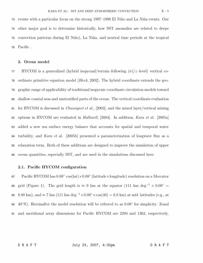
An eddy–resolving (≈ 9 km resolution at the equator and ≈ 7 km9

resolution at mid–latitudes) HYbrid Coordinate Ocean Model (HYCOM),10

configured for the Pacific Ocean (north of 20◦S) is used for examining deep11

atmospheric convection and its relation to sea surface temperature (SST) anoma-12

lies during during 1993 through 2003. The model is forced with high tem-13

poral resolution (6 hourly) atmospheric data from the European Centre for14

Medium–Range Weather Forecasts (ECMWF). The model SST analyses re-15

veal that SST anomalies are strongly related to precipitation anomalies over16

the central and eastern tropical Pacific during La Nina events, and there-17

fore can be used as a proxy for deep convection event. However, no such re-18

lationship is found during the El Nino and neutral phases for the period of19

1993–2003. Thus, the La Nina–related convection events contribute to co-20

herent SST anomaly patterns. Validity of the results are confirmed by eval-21

uating model SST in comparison to satellite–based products over the Pacific22

Ocean. HYCOM simulation with no assimilation of any SST gives a basin-23

averaged monthly mean bias of 0.3◦C and RMS difference of 0.6◦C over the24

North Pacific Ocean during 1993–2003. However, limitations in the atmo-25

spheric forcing (specifically net shortwave radiation) can have substantial im-26

pact on SST, especially during the 1998 La Nina event. Finally, output from27

the eddy–resolving Pacific HYCOM, as presented here, is made available to28

users of interest for many types of applications.29


KARA ET AL.: SST AND DEEP ATMOSPHERIC CONVECTION X - 3

1. Introduction

SST is a key characteristic of ENSO events because a marked shift in equatorial Pacific30

Ocean SST anomalies occurs between the warm (El Nino) and cold (La Nina) phases of31

ENSO [McPhaden, 1999]. For example, the 1997 El Nino event developed very rapidly,32

with a record high SST anomaly occurring in the equatorial Pacific and the abrupt 199833

transition to La Nina resulted in particularly cold SST values. The inter–annual variability34

in tropical Pacific SST is primarily linked to ENSO events [Trenberth et al., 1998] but other35

variations in atmospheric climate also play a role [Enfield, 1996].36

The large variations in strength and evolution of ENSO events make tropical Pacific37

SST simulation by an ocean general circulation model (OGCM) a great challenge on inter–38

annual time scales. Challenges in predicting SST are even more serious for coupled ocean–39

atmosphere predictions. For instance, Barnston et al. [1999] presented inter-comparisons40

of eight dynamical (coupled atmosphere–ocean) and seven statistical models during the41

1997–1998 event, demonstrating that none of them had forecasted the extent of the 199742

El Nino. Besides ENSO events, simulating realistic variability in the amplitude of the43

seasonal SST cycle is also crucial in the Kuroshio–Oyashio Extension in the northwest44

Pacific Ocean, a region where the mid–latitude North Pacific atmosphere is quite sensitive45

to the SST anomalies on inter-annual time scales [e.g., Schneider et al., 2002]. In addition,46

SST variations induced by biological processes in the Kuroshio–Oyashio Extension are of47

particular importance for coupled atmosphere–ocean studies and climate modeling [Miller48

et al., 2004].49



ENSO events have considerable impact on the global climate on both short (e.g., daily)50

and longer (e.g., monthly) time scales and can result in potential socio–economic damages51

[e.g., Elsner and Kara, 1999; Hendon, 2003]. Reliable determination of SST from dynam-52

ical models is of particular importance in the Pacific Ocean. One test for the accuracy53

of ocean models is to determine whether they are able to replicate past ENSO events.54

This capability is relevant to the ENSO events by the delayed oscillator mechanism which55

provides a theoretical basis for the role of the ocean memory in the tropical Pacific climate56

system [e.g., Neelin and Jin, 1993].57

Simulating SST anomalies during ENSO events presents a great challenge for an58

atmospherically–forced OGCM. For example, there is a well–known east–west asymmetry59

where a warm (cold) SST anomaly in the east associated with cold (warm) one in the west60

in the equatorial Pacific [Nakajima et al., 2004]. The asymmetry in inter–annual varia-61

tions of SST depends on heat flux variations at the surface along with radiative and cloud62

feedbacks [Mitchell and Wallace, 1992]. In OGCM simulations the solar radiation fields63

used in the atmospheric forcing are typically obtained from atmospheric models. The ac-64

curacy of these radiation fields is adversely impacted by errors in the extensive equatorial65

cloudiness [e.g., Allan et al., 2004]. In turn, the delayed oscillator mechanism indicates66

that the dynamical adjustments due to the atmospheric forcing in the eastern equatorial67

Pacific basin affect SST whose anomalies usually do not propagate systematically [e.g.,68

Schopf and Suarez, 1987], again making SST simulation from OGCMs a challenging task69

in the equatorial Pacific.70

Along the lines mentioned above, the major objective of this paper is to investigate71

SST anomalies in connection with possible convection events during the historical ENSO72



events with a particular focus on the strong 1997–1998 El Nino and La Nina events. Our73

other major goal is to determine historically, how SST anomalies are related to deepe74

convection patterns during El Nino), La Nina, and neutral time periods at the tropical75

Pacific .76

2. Ocean model

HYCOM is a generalized (hybrid isopycnal/terrain–following (σ)/z–level) vertical co-77

ordinate primitive equation model [Bleck, 2002]. The hybrid coordinate extends the geo-78

graphic range of applicability of traditional isopycnic coordinate circulation models toward79

shallow coastal seas and unstratified parts of the ocean. The vertical coordinate evaluation80

for HYCOM is discussed in Chassignet et al., [2003], and the mixed layer/vertical mixing81

options in HYCOM are evaluated in Halliwell, [2004]. In addition, Kara et al. [2005a]82

added a new sea surface energy balance that accounts for spatial and temporal water83

turbidity, and Kara et al. [2005b] presented a parameterization of longwave flux as a84

relaxation term. Both of these additions are designed to improve the simulation of upper85

ocean quantities, especially SST, and are used in the simulations discussed here.86

2.1. Pacific HYCOM configuration

Pacific HYCOM has 0.08◦ cos(lat)×0.08◦ (latitude×longitude) resolution on a Mercator87

grid (Figure 1). The grid length is ≈ 9 km at the equator (111 km deg−1× 0.08◦ =88

8.88 km), and ≈ 7 km (111 km deg−1×0.08◦×cos(40) = 6.8 km) at mid–latitudes (e.g., at89

40◦N). Hereinafter the model resolution will be referred to as 0.08◦ for simplicity. Zonal90

and meridional array dimensions for Pacific HYCOM are 2294 and 1362, respectively.91



Performing a 1–month simulation took ≈ 18 wall–clock hours on 297 IBM SP POWER392

processors.93

The model includes 20 hybrid layers in the vertical. The top 10 layers may become94

z or sigma levels. The layer structure was chosen such that the first 5 are z–levels to95

help resolve the mixed layer, but this varies regionally. In general, HYCOM needs fewer96

vertical coordinate surfaces than say, a conventional z–level model, because isopycnals97

are more efficient in representing the stratified ocean, as further discussed in Kara et98

al. [2005a]. The density difference values were chosen, so that the layers tend to become99

thicker with increasing depth, with the lowermost abyssal layer being the thickest. The100

K–Profile Parameterization (KPP) mixed layer model [Large et al., 1994] is used in the101

model simulation.102

2.2. Atmospheric forcing

HYCOM reads in the following time–varying atmospheric forcing fields: wind forcing103

(zonal and meridional components of wind stress, wind speed at 10 m above the sea104

surface) and thermal forcing (air temperature and air mixing ratio at 2 m above the105

sea surface, precipitation, net shortwave radiation and net longwave radiation at the sea106

surface). All these climatological monthly mean wind and thermal forcing parameters107

were formed from 1.125◦×1.125◦ ECMWF Re–Analysis (ERA–15) over 1979–1993. Note108

that the wind forcing includes 6–hr variability [Wallcraft et al., 2003; Kara et al., 2003]. A109

simulation which was repeated with a similar atmospheric forcing constructed from ERA-110

40 during 1979-2002 would not yield any notable differences based on our experience with111

the coarser (0.72◦) resolution global HYCOM results.112



Additional forcing parameters read into the model are monthly mean climatologies of113

satellite–based attenuation coefficient for Photosynthetically Active Radiation (kPAR in114

1/m) and river discharge values. The shortwave radiation at depth is calculated using115

a spatially varying monthly kPAR climatology as processed from the daily–averaged k490116

(attenuation coefficient at 490 nm) data set from Sea–viewing Wide Field–of–view Sen-117

sor (SeaWiFS) spanning 1997–2001. Thus, using ocean color data, the effects of water118

turbidity are included in the model simulations through the attenuation depth (1/kPAR)119

for the shortwave radiation. The rate of heating/cooling of model layers in the upper120

ocean is obtained from the net heat flux absorbed from the sea surface down to the depth,121

including water turbidity effects [Kara et al., 2005a].122

The model treats rivers as a “runoff” addition to the surface precipitation field. The123

flow is first applied to a single ocean grid point and smoothed over surrounding ocean grid124

points, yielding a contribution to precipitation in m s−1. This works independently of any125

other surface salinity forcing. Monthly mean river discharge values were constructed at126

NRL. This river data set comes from Perry et al. [1996] which had one annual mean value127

for each river but the set was converted to monthly values using other data sources for128

use used in ocean modeling studies [Barron and Smedstad, 2002].129

Latent and sensible heat fluxes at the air–sea interface are not taken directly from130

ECMWF due to their uncertainties. They are calculated using the model’s top layer (top131

3 m) temperature at each model time step with efficient and computationally inexpensive132

bulk formulas, whose exchange coefficients are expressed as polynomial functions of air–133

sea temperature difference, air–sea mixing ratio difference, and wind speed at 10 m to134

parameterize stability [Kara et al., 2005c]. Including air temperature and model SST135



in the formulations for latent and sensible heat flux automatically provides a physically136

realistic tendency towards the correct SST in the model simulations [Wallcraft et al., 2003].137

The radiation flux (net shortwave and net longwave fluxes at the sea surface) depends on138

cloudiness and is taken directly from ECMWF for use in the model. The input ECMWF139

black–body radiation is corrected within HYCOM to allow for the difference between140

ECMWF and HYCOM SSTs as further discussed in Kara et al. [2005b].141

2.3. Model simulations

The HYCOM simulations were performed with no assimilation of any oceanic data.142

There is only weak relaxation to sea surface salinity to keep the evaporation–precipitation143

budget on track in the model. We realistic bottom topography constructed from the Earth144

Topography Five Minute Grid (ETOP05) (see Kara et al., [this issue]). The model was145

initialized from the Generalized Digital Environmental Model (GDEM) climatology of146

the U.S. Navy at 0.16◦ resolution for computational efficiency. After running HYCOM for147

eight years, the simulation was continued at 0.08◦ resolution until it reached near statisti-148

cal equilibrium (about 28 years) using climatological monthly mean thermal atmospheric149

forcing, but with wind forcing that includes the 6–hr variability (details provided in Kara150

et al. [2005a]). This variability needs to be added because mixed layer is sensitive to151

variations in surface forcing on time scales of a day or less [Sui et al., 2002]. Previously,152

Kara et al. [2005d] also demonstrated the importance of using high–frequency (hybrid)153

wind forcing as opposed to monthly mean wind forcing in HYCOM simulations in simu-154

lating SST. After the spin–up, the climatologically–forced Pacific simulation was extended155

inter–annually (1990–2003) using 6 hourly wind and thermal forcing from ECMWF. In156

this paper, only SST variability during historical ENSO events is investigated. Other157



aspects of inter–annual variability are not the major focus of this paper, since they are158

extensively discussed in Kara et al. [this issue].159

3. Climatological SST in the Pacific Ocean

We first examine accuracy of SSTs obtained from climatologically–forced HYCOM sim-160

ulations. Monthly mean SST from the model is first validated against satellite–based161

Pathfinder and MODAS SST climatologies. The use of two different data sets for the162

HYCOM validation will help to indicate whether or not the deficiencies of model sim-163

ulations at certain regions, such as the equatorial Pacific Ocean and the ice–free high164

northern latitudes), are directly related due the model simulation or to the data set used165

for validating the model. The dual validation will also better determine accuracy of model166

results. A brief explanation of both data sets is given along with the statistical metrics167

used for the model validation.168

The Pathfinder climatology is an update of Casey and Cornillon [1999] and is generated169

using the same techniques [K. Casey, 2006, personal communication]. It has finer spatial170

resolution than the previous version (4 km rather than 9 km) and an improved land mask171

which allows for more retrievals along coastlines and in lakes. The monthly climatology172

covers 1985–2001 as directly provided by the originator. This climatology does not take173

the existence of ice into account (i.e., treats it as a data void). Thus, we added the National174

Oceanic Atmospheric Administration (NOAA) ice climatology [Reynolds et al., 2002] to175

the Pathfinder SST climatology. This is done for each month. Ice–free regions over176

the global ocean are determined from the ice land mask from the NOAA climatology.177

Similarly, the monthly mean MODAS SST climatology is based on Advanced Very–High178

Resolution Radiometer (AVHRR) Multi–Channel SST (MCSST) as described in in Kara179



and Barron [2007]. Mean SST for each month is then obtained using daily SSTs from 1993180

to 2004. Finally, the mean January SST climatology is formed using monthly January181

SSTs over 11 years, and the same process is repeated for other months to construct182

the mean MODAS climatology. Both the Pathfinder and MODAS climatologies were183

interpolated to the Pacific HYCOM grid for comparisons with the model SSTs. As should184

be expected, these climatological data sets are subject to their own unique biases.185

For comparisons with the Pathfinder and MODAS climatologies, monthly mean186

HYCOM SST climatologies are constructed using daily model SST output from the187

climatologically–forced simulation. The model output was archived as a daily snapshot188

rather than a daily mean. We obtained results required to support the conclusions of the189

study with no need to beat down the noise by spatially or temporally averaging (smooth-190

ing) the model output. Thus, monthly means were formed using daily snapshots. At least191

a 7–year mean was needed because in some regions HYCOM with 0.08◦ resolution has192

a strong nondeterministic component due to mesoscale flow instabilities. Monthly mean193

HYCOM SST fields are then compared to the Pathfinder and MODAS climatologies at194

each model grid point over the model domain.195

A set of statistical metrics used for the model SST validation procedure includes mean196

error (ME), root–mean–square (RMS) SST difference, correlation coefficient (R) and non–197

dimensional skill score (SS). Let Xi (i = 1, 2, · · · , 12) be the set of monthly mean MODAS198

(or Pathfinder) reference (observed) SST values from January to December, and let Yi (i =199

1, 2, · · · , 12) be the set of corresponding HYCOM estimates at a model grid point. Also200

let X(Y ) and σX(σY ) be the mean and standard deviations of the reference (estimated)201

values, respectively. The statistical relationships [Murphy, 1995] between MODAS (or202



Pathfinder) and HYCOM SST time series at a given grid point is expressed as follows:203

ME = Y − X, (1)

RMS =

[

1

n

n∑

i=1

(Yi − Xi)2

]1/2

, (2)

R =1

n

n∑

i=1

(Xi − X) (Yi − Y ) / (σX σY ), (3)

SS = R2− [R − (σY /σX)]2

︸︷︷︸

Bcond

− [(Y − X)/σX ]2︸︷︷︸

Buncond

. (4)

We evaluate SST time series between HYCOM and MODAS (or Pathfinder) over the204

annual cycle, so n is 12 at a given grid point. The interested reader is referred to Kara et205

al [this issue] for a detailed description of each statistical metric. The non–dimensional206

metric, SS, is considered to be the most important one because it takes both conditional207

bias (the one due to differences in standard deviations) and unconditional bias (i.e., the208

one due to differences in means) into account between the two time series. SS is 1.0209

(negative) for perfect (poor) HYCOM SST simulations.210

3.1. SST errors

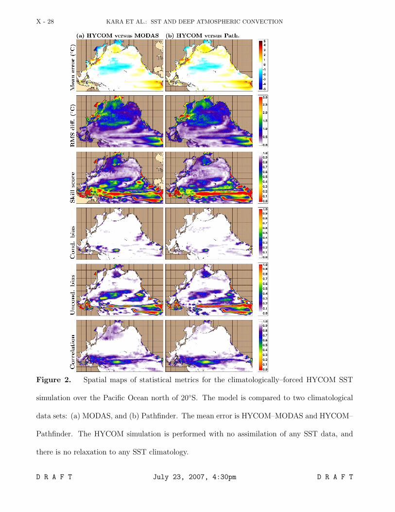
Figure 2 shows results of statistical comparisons of HYCOM SST to the MODAS and211

Pathfinder SST climatologies. In particular, for the given atmospheric wind and thermal212

forcing from ECMWF, annual mean SST bias presented by mean error maps clearly reveals213

that HYCOM is able to simulate SST with small errors (within ±0.5◦C) over the most214

of Pacific Ocean. Cold (warm) model SST biases are in blue (red). Overall, SST biases215

(i.e., HYCOM–MODAS and HYCOM–Pathfinder) are almost the same regardless of the216

climatology used for validating the model, except that there are some differences at high217

latitudes.(Figure 3).218



Large errors between HYCOM and MODAS SST are less evident between HYCOM and219

Pathfinder SST at these high latitude belts. The reason is that the MODAS climatology220

lacks a realistic ice field, resulting in warmer model SST than MODAS by > 2◦C. On the221

contrary, when HYCOM is compared to the Pathfinder climatology, the same biases are222

largely reduced because we added a realistic ice climatology, as explained above, to the223

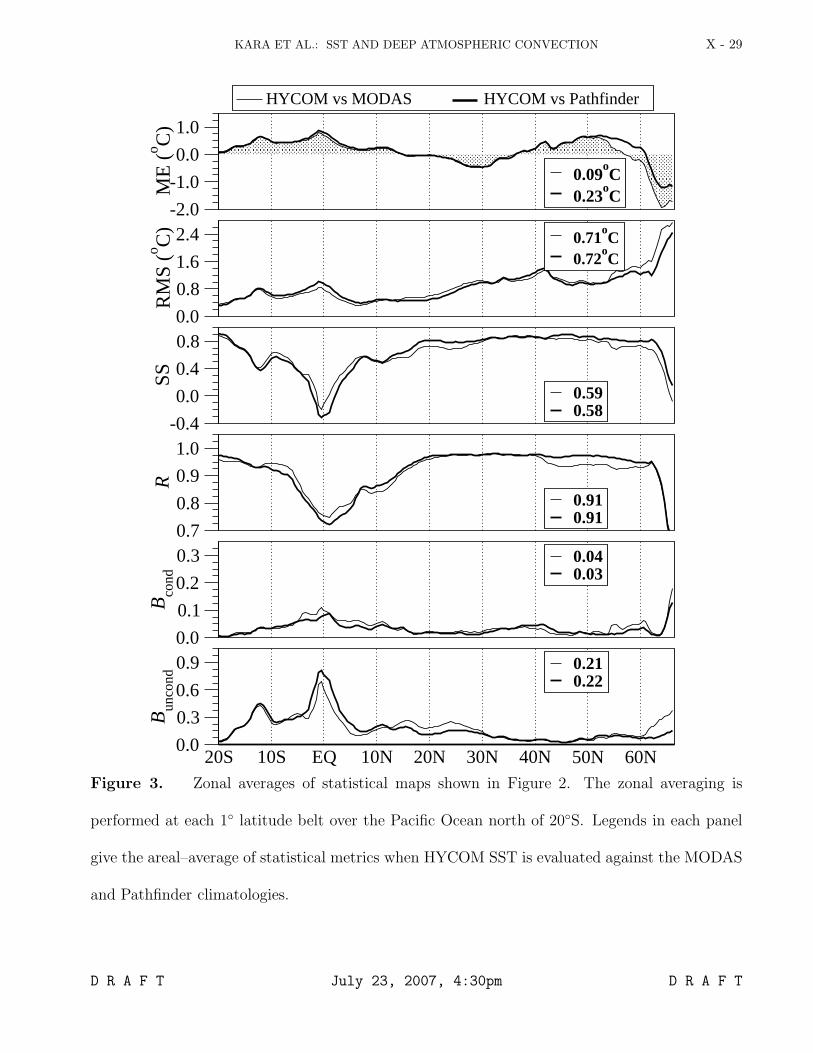
Pathfinder climatology. The model generally gives a small RMS SST difference of ≈<224

0.8◦C calculated over the seasonal cycle (Figure 2). In fact, the basin–wide areal–average225

of RMS SST is 0.71◦C (0.72◦C) when the climatologically–forced HYCOM simulation is226

validated against MODAS (Pathfinder) SST climatology. The RMS SST difference is227

usually small (large) near the equatorial regions (north of 40◦N). However, the model has228

low (high) skill at the equator (north of 40◦N) as seen from Figure 3. The reason is that229

the amplitude seasonal of the seasonal cycle of SST is quite different in the two regions230

(much smaller in the tropics) so a non–dimensional metric is required to better evaluate231

model skill in simulating the mean and seasonal cycle of SST (see also the results for R,232

correlation coefficient).233

Biases are taken into account in the RMS differences, but in some cases the latter can234

be small when skill and correlation are poor. This can occur where the amplitude of the235

seasonal cycle is small, giving a small RMS SST difference but also low skill, as in the236

western equatorial Pacific warm pool (Figure 2). Note that skill score takes biases into237

account, something not done by correlation coefficient. Near the equatorial Pacific the238

biases between HYCOM and MODAS (or Pathfinder) SST time series over the seasonal239

cycle are due mostly to differences in the mean (i.e., large unconditional bias).240



3.2. Climatologically– versus inter–annually–forced simulations

Results presented in the companion paper [Kara et al. this issue] demonstrate that241

monthly mean SST simulations from HYCOM using the inter–annual atmospheric forcing242

are very reliable in comparison to the observations. This is particularly true over the most243

of the Pacific on short (e.g., daily) and longer (monthly and annual) time scales. A par-244

ticular question arises here, “what is the accuracy of climatologically–forced simulations245

presented in section 3 with respect to the climatology of the inter–annually–forced HY-246

COM simulations“? The answer to this question would reveal whether or not the monthly247

climatological atmospheric forcing produces the monthly mean climatological ocean state,248

an important result that any ocean modeler performing long–term simulations would be249

interested in knowing.250

For the inter–annual model simulations, the initial assumption is that monthly mean251

climatological atmospheric forcing (with 6–h wind anomalies, but no other atmospheric252

forcing anomalies) would give the monthly mean climatological ocean state. A comparison253

of the long term monthly mean SSTs from 1993 to 2004 from the inter–annually–forced254

HYCOM simulations with those from the climatologically–forced simulation largely con-255

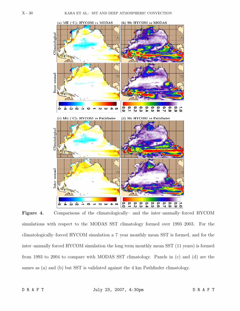
firms the validity of this assumption buth with some noteworthy exceptions, e.g., more256

(less) accurate results from the inter–annual simulation in the subtropical (subpolar) gyre257

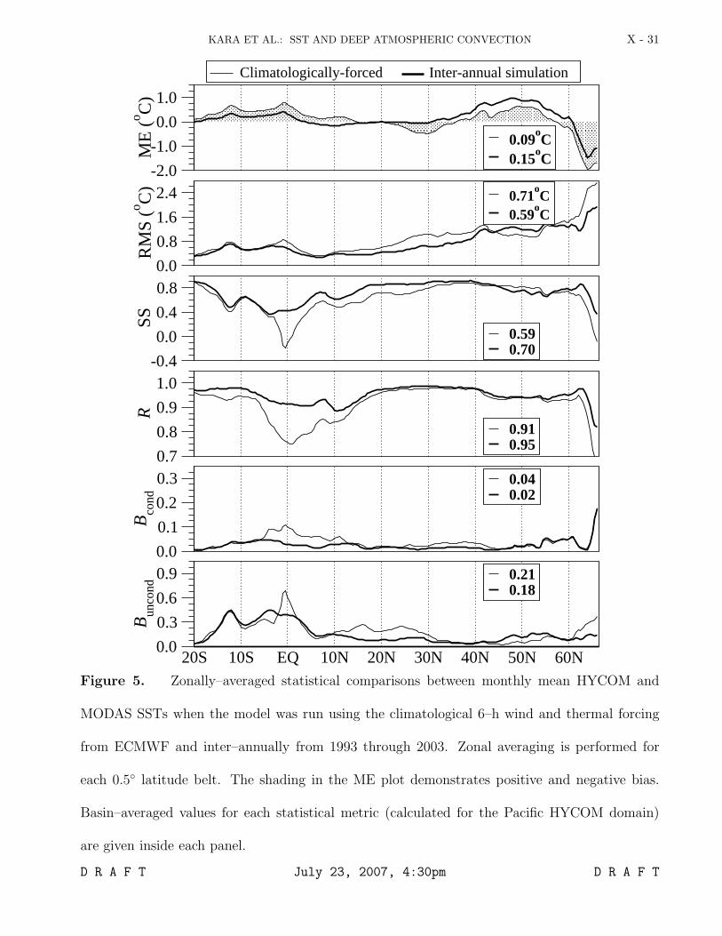
(Figure 4). However, the inter–annual simulation generally gives slightly better SSTs at258

most latitude belts (Figure 5), with much high correlation and skill score in the equator.259

As confirmed above by comparing the climatologically– and inter–annually– forced260

model simulations, HYCOM has the ability to replicate not only the past SST events but261

also the climatology in a consistent way. This is a critical requirement for OGCM studies262



that are developed for both short and long term climate studies. If the climatologically–263

and inter–annually–forced model simulations gave significantly different results then we264

would have to re–assess our strategy of using monthly winds with 6–h anomalies and265

monthly mean thermal forcing. One reason why wind anomalies are enough is that they266

are sufficient for the bulk parameterization to give 6–h variability in the total heat flux267

as evident from the accuracy of SST validation statistics.268

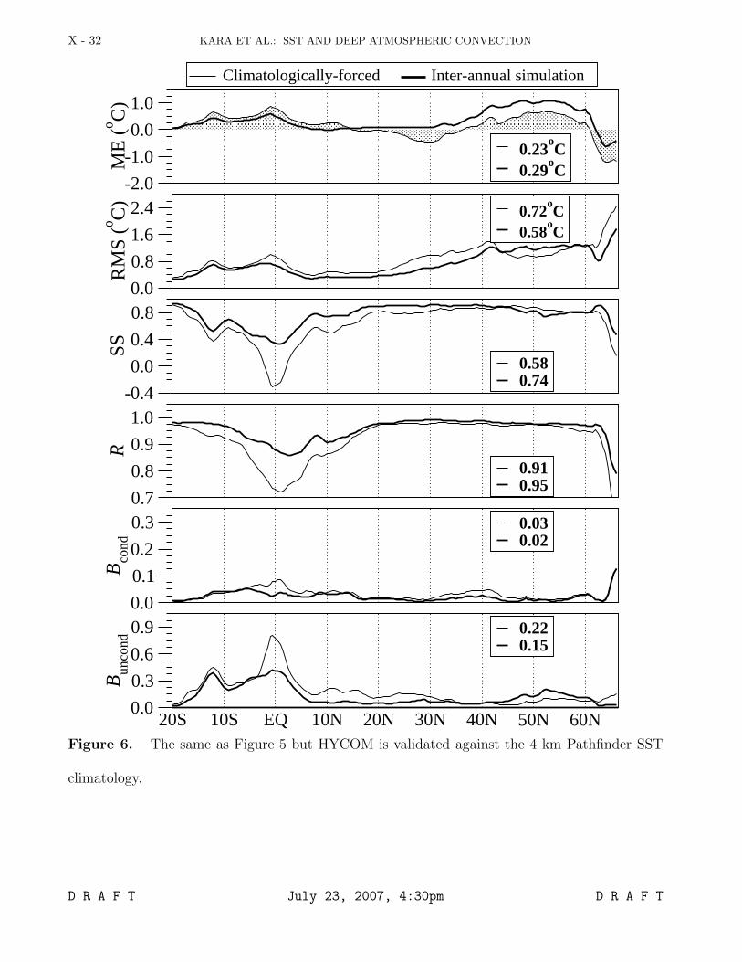
The same validation procedure for both HYCOM simulations is repeated using the269

4 km Pathfinder SST climatology (Figure 4c,d). This data set was formed using the same270

techniques as in Casey and Cornillon [1999] but on the newer ≈ 4 km data (rather than271

≈ 9 km) over 1985–2001. Zonally averaged statistical results remain almost the same when272

validating HYCOM against the Pathfinder SST climatology (Figure 6), in comparison to273

those shown in Figure 5 except that the annual mean bias is slightly increased (0.09◦C274

to 0.23◦C for the climatologically–forced simulation and 0.15◦C to 0.29◦C for the inter–275

annual simulation).276

HYCOM SST errors with respect to the MODAS climatology are generally large in277

high northern latitudes (Figure 4). This is due partly to the fact that the MODAS data278

has a lack of ice in these regions (see also section 3). Errors due to the model circulation279

(e.g., in the Japan/East Sea) and atmospheric forcing (e.g., off the California coast)280

also contribute in accurate simulation of SST (see Kara et al., [this issue] for detailed281

discussions). However, the model errors are significantly reduced in these regions when the282

Pathfinder SST climatology is used for the validation. Note that the original Pathfinder283

SST climatology includes neither a specific ice climatology nor a clear separation between284

an ice values and a data void. Even though the Pathfinder climatology (unlike the inter–285



annual Pathfinder SST data set) is gap filled, there are places, such as parts of the Arctic286

and inland waters, where the Pathfinder SST are not very reliable. For this reason, as287

mentioned previously, we modified the Pathfinder climatology, so that the new Pathfinder288

SST uses the ice concentration climatology from NOAA to decide if a data void should be289

treated as ice. When HYCOM is validated against this new climatology, there is a clear290

indication of the fact that the model does in fact simulate SST in ice–covered regions even291

though there is no explicit coupling with any ice model.292

4. Historical ENSO Events

The time period, during which daily and monthly SST variations were discussed in the293

companion paper also includes ENSO events, whose detailed examination is the primary294

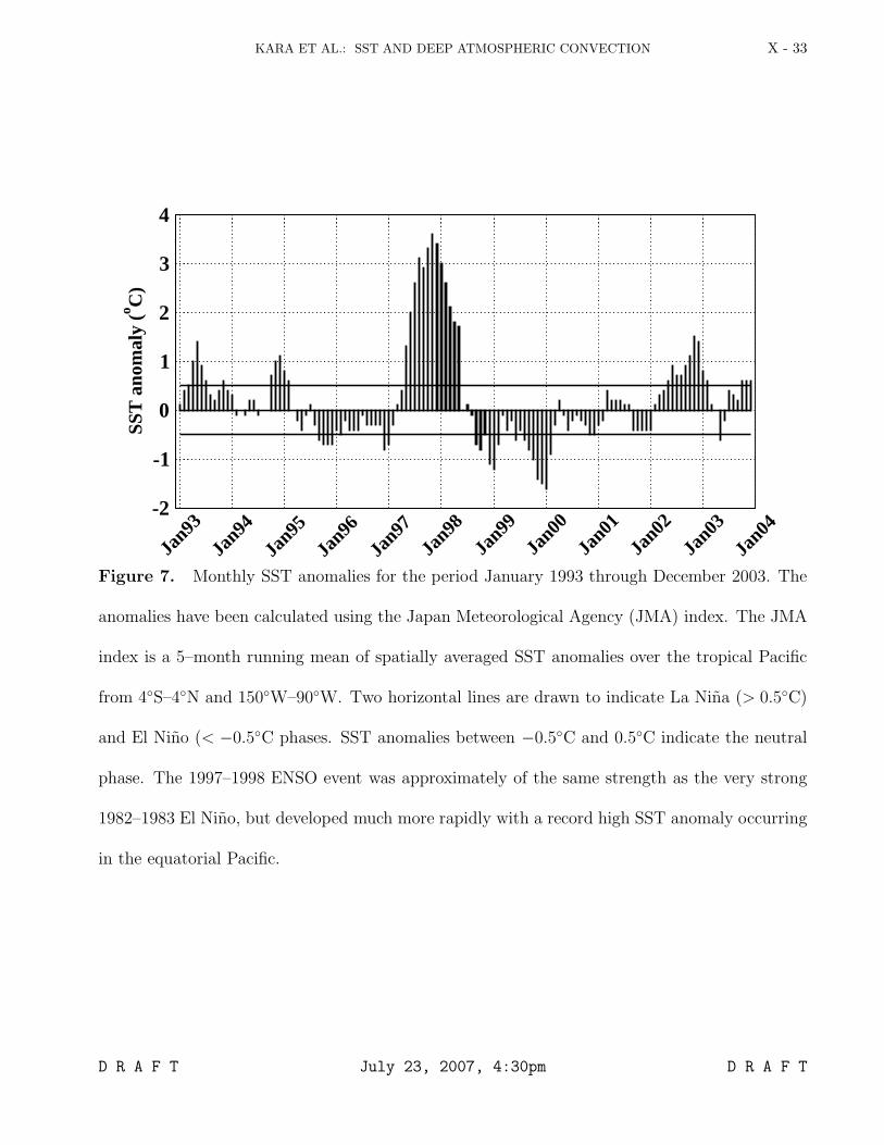
focus of this section. Monthly mean SST anomalies from 1993 through 2003 are shown in295

Figure 7 and based the Japan Meteorological Agency (JMA) index [Hanley et al., 2003].296

El Nino (La Nina) period is described when monthly SST anomaly is > 0.5◦ (< 0.5◦).297

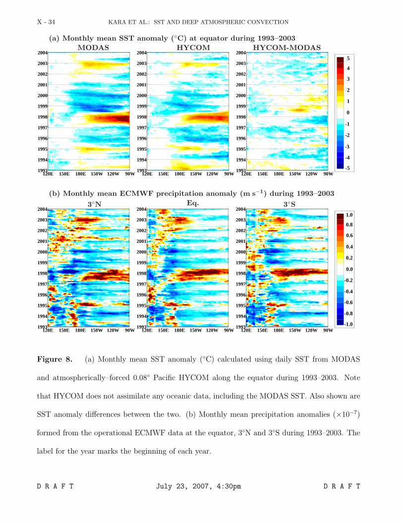
Monthly mean SST anomaly fields are constructed from MODAS and HYCOM along298

the equatorial Pacific (at 0◦) from 1993 to 2004 (Figure 8a). The cold and warm SST299

anomalies in the eastern and central Pacific are evident from MODAS, and reasonably300

reproduced by HYCOM. The basin–averaged RMS SST anomaly difference with respect301

to the MODAS SST anomaly is 0.46◦C along the equator during 1993–2003. The SST302

anomaly even reached a value > 4◦C in the eastern equatorial Pacific when the strong303

1997 El Nino was in progress. These large warm anomalies are seen in both MODAS and304

HYCOM, while the latter has a small cold bias of 0.5◦ to 1.0◦C along the easternmost305

part of equator. Consistent with MODAS the model is able to simulate the extent and306

magnitude of warm SST anomalies for the El Nino years of 1997 and 2002 reasonably307



well. While the model SST anomaly is ≈ 0.5◦C too warm during the 1999 La Nina event,308

there was almost no model SST bias during the 1998 La Nina event.309

4.1. Atmospheric Deep Convection

To investigate the impact of the ENSO signals on convection events in connection with310

SST anomalies in the equatorial Pacific, monthly mean precipitation anomalies are formed311

from ECMWF operational model output during 1993–2003 (Figure 8b). Precipitation312

anomalies along 3◦N, the equator and 3◦S generally resemble each other. On the other313

hand, some relatively large and positive precipitation anomalies that exist at 3◦N and314

equator do not exist at 3◦S during the middle months of 1997. As typically seen in315

regions with warm water such as at and north of the Inter–tropical Convergence Zone316

(ITCZ) [e.g., Cronin et al., 2006], this implies that the expected southward migration of317

ITCZ to the warmest sea surface areas is disrupted due to the unusually warm sea surface318

temperatures which occurred in the easternmost Pacific at the beginning of the 1997 El319

Nino. The southward movement of ITCZ to 3◦S was therefore restricted, resulting in less320

precipitation.321

Positive precipitation anomaly (higher than average rainfall) is a strong indication of322

above average cloudiness in Figure 8b. Thus, precipitation can be considered as a measure323

of atmospheric convection. While the outgoing long wave radiation (OLR) could also324

be used for identifying the convection events, it is not preferred here because satellites325

cannot penetrate clouds when measuring OLR. Traditionally, deep atmospheric convection326

is expected near/around the western equatorial Pacific warm pool (between 160◦E and327

160◦W), where the strongest inter–annual coupling between atmosphere and ocean occurs328

and inter–annual heating of the atmosphere is greatest [Clarke and Van Gorder, 2001].329



This is not surprising because a necessary condition for the development and persistence330

of deep convection (i.e., enhanced cloudiness and precipitation) is to have SSTs > 28◦C331

[e.g., Holton, 1992]. As expected, warm pool SSTs are typically warmer than that specific332

value (see Figure 2 in the companion paper).333

Variations in the SST of the warm pool and the location of its eastern edge are also334

reflected in the precipitation anomalies even when SST anomalies are small. In addition335

to the warm pool regions, the atmospheric convection anomalies extended east of 160◦E336

in many years (besides El Nino years) as evident from positive precipitation anomalies337

(Figure 8b). The monthly SST in these regions is generally larger than > 28◦C with338

the warm water extending east of the warm pool, i.e., when the warm water extended339

eastward, the deep atmospheric convection moved with it, carrying the weak precipitation340

anomaly signal with it. Note that the SST anomalies generally diminish in regions where341

convection persists (Figure 8a,b).342

One may argue that the largest SST anomalies are generally seen in the eastern equato-343

rial Pacific from 1993 to 2004 (Figure 8a), while the strong convection anomalies usually344

occurred in the western and central equatorial Pacific from 2000 to 2004. This is because345

SST is generally much colder in the eastern equatorial Pacific than the western Pacific346

warm pool so that larger (and less common) anomalies are required to attain the threshold347

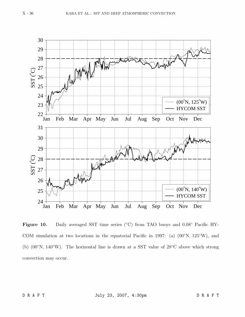
SST. The 1997 El Nino event, that resulted in anomalously high rainfall in the central348

and eastern equatorial Pacific for about a year, is an exception. During this time the SST349

in the equatorial Pacific Pacific remains near or above > 28◦C (Figure 10).350

We investigate whether or not time periods with changes in SST (i.e., colder or warmer)351

are related to those in precipitation anomalies at the tropical Pacific. This is done during352



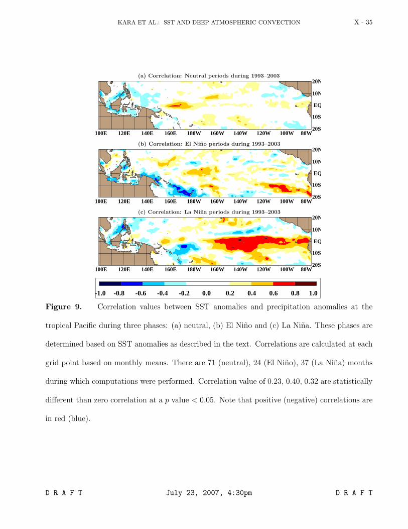
El Nino, La Nina and neutral time periods, separately. There are 24, 37 and 71 months353

when warm, cold and neutral phases occurred during 1993–2003. SST anomalies from the354

model and precipitation anomalies from ECMWF are grouped for each phase separately,355

and correlations are then calculated. As evident from Figure 9, an increase or decrease in356

SST anomalies are strongly related to changes in precipitation anomalies only during La357

Nina events but only at the eastern and central equatorial Pacific. The enhanced deep358

convection associated with divergences and upwelling in this region indicates that precipi-359

tation anomalies have direct effect on cold SSTs. This also confirms that as the convection360

moved eastward (Figure 8b), enhanced low–level instability does not cause strong convec-361

tion over the region of the cold SSTs, i.e., there was relatively weak convective activity362

over the central and eastern Pacific.363

4.2. The 1998 ENSO Transition

OGCMs are expected to simulate realistic SSTs not only in regions where SST is dom-364

inated by local forcing and vertical mixing (e.g., western Pacific warm pool) but also in365

those where SST cooling is mostly a result of upwelling rather than mixing (e.g., eastern366

equatorial Pacific). For this reason we analyze SST variability during the 1998 transition367

from El Nino to La Nina in the eastern and central equatorial Pacific where strong up-368

welling can have a large impact on the upper ocean circulation and thermal structure,369

including SST.370

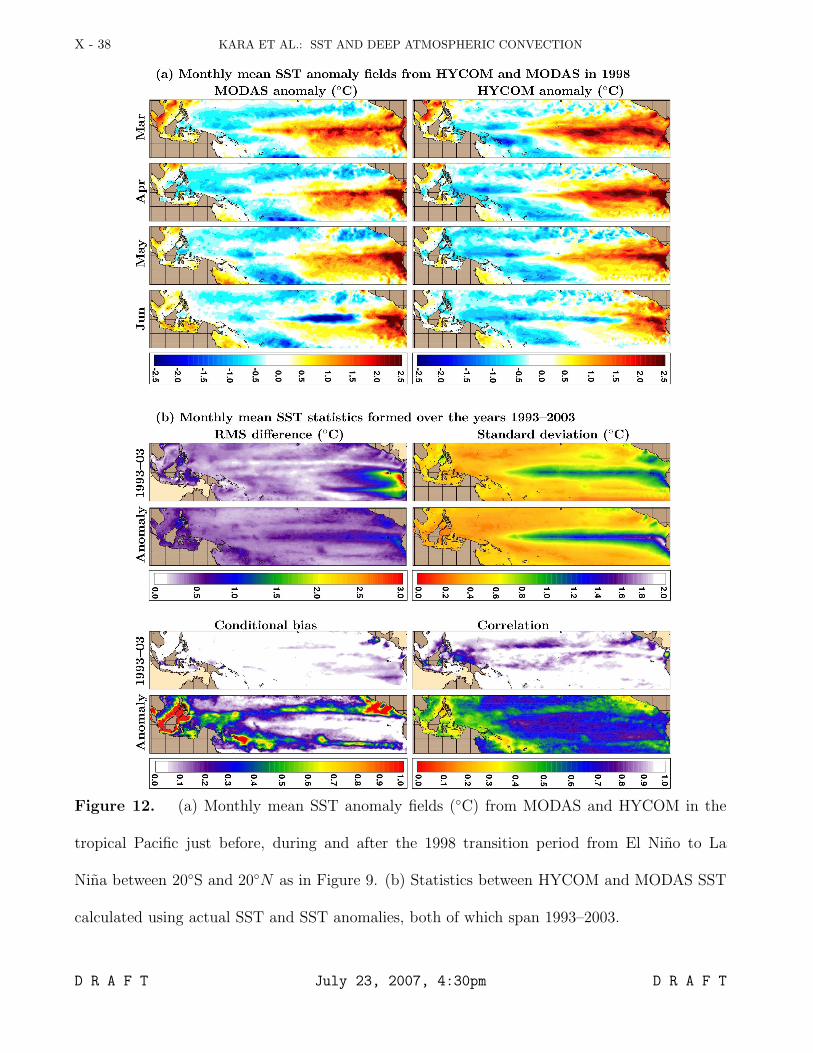
We first examine spatial anomaly fields of SST instead of full SST fields. Such an371

analysis is particularly useful in situations where monthly SST variations may reach a372

peak, as in the strong 1998 transition period from El Nino to La Nina. To form anomalies,373

mean SST is formed for each month from 1993 to 2004, and this long term monthly SST374



is subtracted from SST for a given month of the year. This is done for both MODAS and375

HYCOM. In general, HYCOM is able reproduce the extent and magnitude of monthly376

mean warm (cold) SST anomalies reasonably well during the 1998 transition even with no377

assimilation of or relaxation to SST (Figure 12a). On the other hand, the SST anomaly378

from HYCOM is > 1◦C warmer than that from MODAS during June 1998, the beginning379

of the 1998 La Nina. When the error statistics are calculated over the time period from380

1993 to 2004, the model performance in predicting SST anomalies is slightly worse than381

that in predicting the actual SSTs (Figure 12b). This is due likely to the fact that time382

period period chosen (1993 to 2004) is not long enough to form anomalies.383

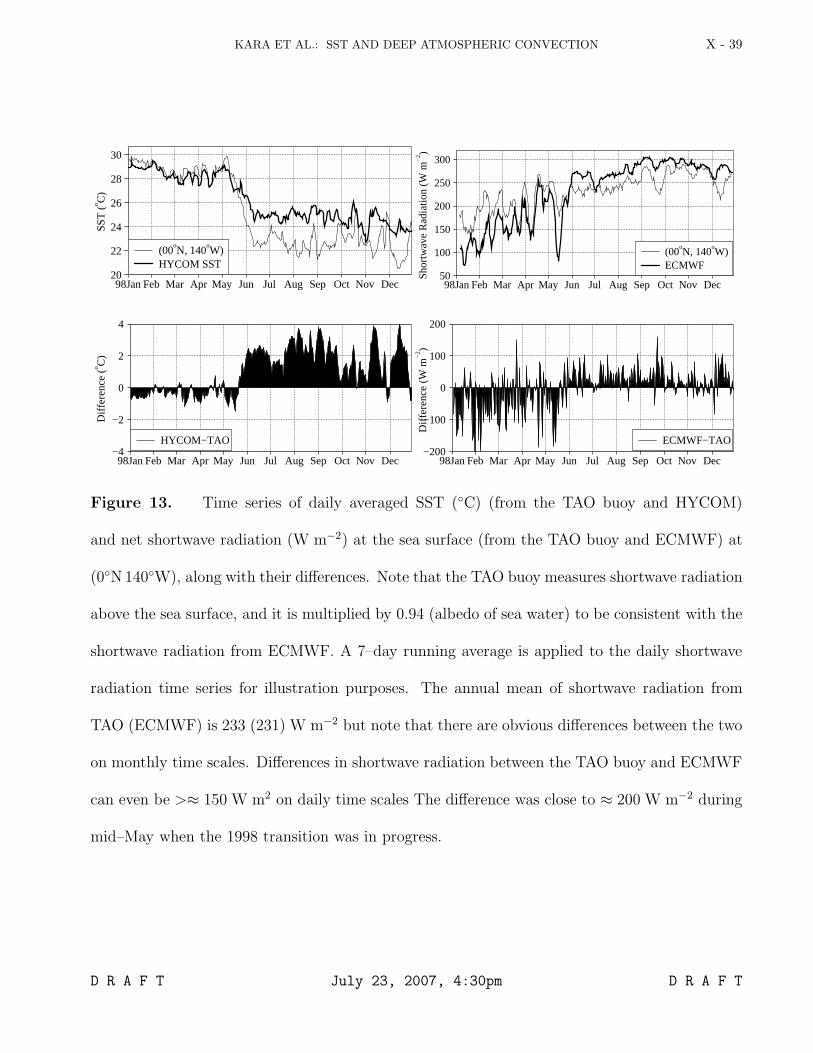
Since the large SST drop of ≈ 7◦C occurred in just a short time period (a month or384

so) as evident from (Figure 11), we analyze SST variations on shorter time scales (daily)385

as opposed to the longer time scales (monthly) during the strong 1998 transition from386

El Nino to La Nina. Interestingly, unlike the monthly mean SST anomalies, Figure 13387

shows that a relatively warm model bias (≈ 2◦C) does exist in the daily SST time series at388

TAO buoys locations (illustrated at (0◦N 140◦W)) during the La Nina phase in 1998. The389

atmospheric forcing from ECMWF is one possible reason that the HYCOM SST anomaly390

is not as cold as the MODAS SST anomaly as will be elaborated below.391

Daily averaged air temperature, wind speed and air mixing ratio from ECMWF used392

for the model simulations were compared to those from TAO buoys at several locations393

in the eastern equatorial Pacific. They generally agreed within reasonable accuracies (not394

shown). However, there were significant differences in net shortwave radiation between395

the buoys and ECMWF, affecting the accuracy of the model results (Figure 13). For396

example, Figure 12a confirmed that the HYCOM SST anomaly is ≈ 0.5◦C warmer than397



MODAS in May and June 1998 at this particular location at the central equatorial Pacific.398

A striking feature evident from Figure 13 is that the shortwave radiation from ECMWF399

is generally underestimated (overestimated) in the first (second) part of 1998, and this is400

probably due to the cloudiness. There were no daily cloud cover measurements from the401

TAO buoy to further confirm this statement.402

5. Conclusions

In this study we demonstrate how an atmospherically–forced OGCM (without cou-403

pling to any atmospheric model) may play an important role in representing the ocean404

component of the climate system on a wide variety of temporal and spatial scales. A spe-405

cific application includes the examination of atmospheric convection events with respect406

to SST anomalies obtained from the 0.08◦ resolution North Pacific HYCOM simulation.407

The monthly mean SST results were obtained from a climatologically–forced HYCOM408

simulation with no assimilation of ocean data, and no relaxation to an SST climatology.409

HYCOM simulations indicate the existence of strong correlations between SST anoma-410

lies and tropical precipitation anomalies (an indicator of convective heating) in the eastern411

and central equatorial Pacific. This occurs when considering La Nina events (37 months)412

from 1993 to 2004, but not for the other time periods, including El Nino and neutral413

phases. Thus, under some circumstances distribution of tropical convective heating can414

have substantial influence in warming or cooling of the SST over the eastern and central415

equatorial Pacific during cold phases of ENSO. In particular, ocean modulates atmo-416

spheric convection through inter–annual SST fluctuations. The relationship between SST417

and convection in the model is found to be close to the observations.418



The model results revealed that it is possible to obtain accurate SST with the use of419

available atmospheric forcing (e.g., ECMWF) for an OGCM (e.g., HYCOM). These accu-420

racies are essential prerequisites for SST assimilation to the model. We also examine the421

predictive capability of HYCOM in simulating SST anomalies, and the role of uncertain-422

ties in the atmospheric forcing. The assumption that using monthly mean climatological423

atmospheric forcing with addition of a 6 hourly wind component would result in realistic424

simulation of the monthly mean climatological SST is demonstrated. In this case the425

inter–annual HYCOM simulation gave a slightly lower basin–averaged RMS SST differ-426

ence of 0.6◦C than the value of 0.7◦C obtained from the climatologically–forced simulation,427

when the model was validated against a satellite–based SST data set over the seasonal428

cycle during 1993–2003.429

The model had difficult time in simulating the equatorial SST anomaly during the430

neutral year of 1994, giving a cold bias of ≈ 1.0◦. This is due partly to the quality of431

atmospheric forcing products in the early time periods. Radiation fields from the archived432

products (such as ECMWF) still have serious problems due to the cloudiness, hampering433

the simulation skill of the ocean model. In this paper, we also placed some emphasis on the434

shortwave radiation from ECMWF which could have serious errors during ENSO events435

due to extensive cloudy time periods. This is confirmed by examining the relationship436

between daily SST and shortwave at the sea surface at a particular TAO buoy location437

on the equator at 140◦W in the eastern Pacific in 1998.438

Finally, an accurate and generalized ocean model capability is in place in the HYCOM439

modeling system. For the benefit of many users, one of our major purposes is to support440

regional and littoral applications, including the capability to provide boundary conditions441



to nested models with fixed depth–z level coordinates, terrain–following coordinates, and442

unstructured grids. Fine resolution model outputs from Pacific HYCOM simulations are443

available online at http://hycom.rsmas.miami.edu/dataserver/.444

Acknowledgments.445

This work was funded by the Office of Naval Research (ONR) under program element446

601153N as part of the NRL 6.1 project, Global Remote Littoral Forcing via Deep Water447

Pathways. The HYCOM simulations were performed on a IBM SP POWER3 at the Army448

Research Laboratory, Aberdeen, Maryland and on a SGI Origin 3900 at the Aeronautical449

Systems Center, Wright–Peterson Air Force Base, Ohio, using grants of high performance450

computer time from the Department of Defense High Performance Computing Modern-451

ization Program. This is contribution NRL/JA/7320/06/7057 and has been approved for452

public release.453

References

Allan, R. P., M. A. Ringer, J. A. Pamment, and A. Slingo (2004), Simulation of the Earth’s454

radiation budget by the European Centre for Medium–Range Weather Forecasts 40-year455

reanalysis (ERA–40), J. Geophys. Res., 109, D18107, doi:10.1029/2004JD004816.456

Barnston, A. G., M. Glantz, and Y. He (1999), Predictive skill of statistical and dynamical457

climate models in SST forecasts during the 1997–98 El Nino and the 1998 La Nina onset,458

Bull. Amer. Met. Soc., 60, 217–243.459

Barron, C. N., and L. F. Smedstad (2002), Global river inflow within the Navy Coastal460

Ocean Model, Proc. to Oceans 2002 MTS/IEEE Conference, 29–31 October 2002, 1472–461

1479.462



Barron, C. N., and A. B. Kara (2006), Satellite–based daily SSTs over the global ocean,463

Geophys. Res. Lett., 33, L15603, doi:10.1029/2006GL026356.464

Bleck, R. (2002), An oceanic general circulation model framed in hybrid isopycnic–465

cartesian coordinates, Ocean Modelling, 4, 55–88.466

Casey, K. S., and P. Cornillon (1999), A comparison of satellite and in situ based sea467

surface temperature climatologies, J. Climate, 12, 1848–1863.468

Chassignet, E. P., L. T. Smith, G. R. Halliwell Jr., and R. Bleck (2003), North Atlantic469

simulations with the HYbrid Coordinate Ocean Model (HYCOM): Impact of the vertical470

coordinate choice, reference pressure, and thermobaricity, J. Phys. Oceanogr., 33, 2504–471

2526.472

Clarke, A. J., and S. Van Gorder (2001), ENSO prediction using an ENSO trigger and473

a proxy for western equatorial Pacific warm pool movement, Geophys. Res. Lett., 28,474

579–582.475

Cronin, M. F., C. W. Fairall, and M. J. McPhaden (2006), An assessment of buoy–derived476

and numerical weather prediction surface heat fluxes in the tropical Pacific, J. Geophys.477

Res., 111, C06038, doi:10.1029/2005JC003324.478

Elsner, J. B., and A. B. Kara (1999), Hurricanes of the North Atlantic: Climate and479

Society, 496 pp, Oxford University Press, New York.480

Enfield, D. B. (1996), Relationships of inter–American rainfall to tropical Atlantic and481

Pacific SST variability, Geophys. Res. Lett., 23, 3305–3308.482

Halliwell, G. R. Jr. (2004), Evaluation of vertical coordinate and vertical mixing algo-483

rithms in the HYbrid Coordinate Ocean Model (HYCOM), Ocean Modelling, 7, 285–484

322.485



Hanley, D. E., M. A. Bourassa, J. J. O’Brien, S. R. Smith, and E. R. Spade (2003), A486

quantitative evaluation of ENSO indices, J. Climate, 16, 1249–1258.487

Hendon, H. H. (2003), Indonesian rainfall variability: Impacts of ENSO and local air–sea488

interaction, J. Climate, 16, 1775–1790.489

Holton, J. E. (1992), An Introduction to Dynamic Meteorology, 511 pp, Academic Press,490

New York.491

Kara, A. B., A. J. Wallcraft, and H. E. Hurlburt (2003), Climatological SST and MLD492

simulations from NLOM with an embedded mixed layer, J. Atmos. Oceanic Technol.,493

20, 1616–1632.494

Kara, A. B., A. J. Wallcraft, and H. E. Hurlburt (2005a), A new solar radiation penetra-495

tion scheme for use in ocean mixed layer studies: An application to the Black Sea using496

a fine resolution HYbrid Coordinate Ocean Model (HYCOM), J. Phys. Oceanogr., 35,497

13–32.498

Kara, A. B., A. J. Wallcraft, and H. E. Hurlburt (2005b), Sea surface temperature sen-499

sitivity to water turbidity from simulations of the turbid Black Sea using HYCOM, J.500

Phys. Oceanogr., 35, 33–54.501

Kara, A. B., H. E. Hurlburt, and A. J. Wallcraft (2005c), Stability–dependent exchange502

coefficients for air–sea fluxes, J. Atmos. Oceanic Technol., 22, 1080–1094.503

Kara, A. B., H. E. Hurlburt, A. J. Wallcraft, and M. A. Bourassa (2005d), Black Sea504

mixed layer sensitivity to various wind and thermal forcing products on climatological505

time scales, J. Climate, 18, 5266–5293.506

Kara, A. B, and H. E. Hurlburt (2006), Daily inter–annual simulations of SST and MLD507

using atmospherically–forced OGCMs: Model evaluation in comparison to buoy time508



series, J. Mar. Sys., 62, 95–119.509

Kara, A. B., A. J. Wallcraft, and H. E. Hurlburt (2007), Land contamination of atmo-510

spheric forcing for ocean models near land–sea boundaries, J. Phys. Oceanogr., 37,511

803–818.512

Kara, A. B., and C. N. Barron (2007), Fine–resolution satellite–based daily sea513

surface temperatures over the global ocean, J. Geophys. Res., 112, C05041,514

doi:10.1029/2006JC004021.515

Large, W. G., J. C. McWilliams, and S. C. Doney (1994), Oceanic vertical mixing: A516

review and a model with a nonlocal boundary layer parameterization, Rev. Geophys.,517

32, 363–403.518

McPhaden, M. J. (1999), Genesis and evolution of the 1997-98 El Nino, Science, 283,519

950–954.520

Miller, A. J., F. Chai, S. Chiba, J. R. Moisan and D. J. Neilson (2004), Decadal–scale521

climate and ecosystem interactions in the North Pacific Ocean, J. Oceanography, 60,522

163–188.523

Mitchell, T. P, and J. M. Wallace (1992), The annual cycle in equatorial convection and524

sea surface temperature, J. Climate, 5, 1140–1156.525

Murphy, A. H. (1995), The coefficients of correlation and determination as measures of526

performance in forecast verification, Wea. Forecasting, 10, 681–688.527

Nakajima, K., E. Toyodo, M. Ishiwatari, S–I. Takehiro, and Y–Y. Hayashi, (2004), Initial528

development of tropical precipitation patterns in response to a local warm SST area:529

An aqua–planet ensemble study, J. Meteor. Soc. Japan, 82,1483–1504.530



Neelin, J.D., and F.–F. Jin (1993), Modes of interannual tropical ocean – atmosphere531

interaction – a unified view. Part II: Analytical results in the weak–coupling limit, J.532

Atmos. Sci., 50, 3504–3522.533

Perry, G. D., P. B. Duffy, and N. L. Miller (1996), An extended data set of river discharges534

for validation of general circulation models, J. Geophys. Res., 101, 21,339–21,349.535

Reynolds, R. W., N. A. Rayner, T. M. Smith, and D. C. Stokes (2002), An improved536

in–situ and satellite SST analysis for climate, J. Climate, 15, 1609–1625.537

Schneider, N., A. J. Miller, and D. W. Pierce (2002), Anatomy of North Pacific decadal538

variability, J. Climate, 15, 586–605.539

Schopf, P. S., and M. J. Suarez (1987), Vacillations in a coupled ocean-atmosphere model,540

J. Atmos. Sci., 45, 549–566.541

Sui, C–H., X. Li, M. M. Rienecker, K–M. Lau, and R. T. Pinker (2002), The role of542

daily surface forcing in the upper ocean over the tropical Pacific: A numerical study, J.543

Climate, 16, 756–766.544

Trenberth, K. E., G. W. Branstator, D. Karoly, A. Kumar, N.–C. Lau, and C. Ropelewski545

(1998), Progress during TOGA in understanding and modeling global teleconnections546

associated with tropical sea surface temperature, J. Geophys. Res., 103, 14,291–14,324.547

Wallcraft, A. J., A. B. Kara, H. E. Hurlburt, and P. A. Rochford (2003), The NRL Layered548

Global Ocean Model (NLOM) with an embedded mixed layer submodel: Formulation549

and tuning, J. Atmos. Oceanic Technol., 20, 1601–1615.550



20S

10S

EQ

10N

20N

30N

40N

50N

60N

100E 120E 140E 160E 180W 160W 140W 120W 100W 80W

3.5

4.0

4.5

5.0

5.5

6.0

6.5

7.0

7.5

8.0

8.5

9.0

9.5

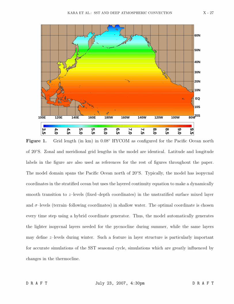
Figure 1. Grid length (in km) in 0.08◦ HYCOM as configured for the Pacific Ocean north

of 20◦S. Zonal and meridional grid lengths in the model are identical. Latitude and longitude

labels in the figure are also used as references for the rest of figures throughout the paper.

The model domain spans the Pacific Ocean north of 20◦S. Typically, the model has isopycnal

coordinates in the stratified ocean but uses the layered continuity equation to make a dynamically

smooth transition to z–levels (fixed–depth coordinates) in the unstratified surface mixed layer

and σ–levels (terrain–following coordinates) in shallow water. The optimal coordinate is chosen

every time step using a hybrid coordinate generator. Thus, the model automatically generates

the lighter isopycnal layers needed for the pycnocline during summer, while the same layers

may define z–levels during winter. Such a feature in layer structure is particularly important

for accurate simulations of the SST seasonal cycle, simulations which are greatly influenced by

changes in the thermocline.



Figure 2. Spatial maps of statistical metrics for the climatologically–forced HYCOM SST

simulation over the Pacific Ocean north of 20◦S. The model is compared to two climatological

data sets: (a) MODAS, and (b) Pathfinder. The mean error is HYCOM–MODAS and HYCOM–

Pathfinder. The HYCOM simulation is performed with no assimilation of any SST data, and

there is no relaxation to any SST climatology.



20S 10S EQ 10N 20N 30N 40N 50N 60N0.0

0.3

0.6

0.9

Bun

cond

0.210.22

0.0

0.1

0.2

0.3

Bco

nd

0.040.03

0.7

0.8

0.9

1.0

R

0.910.91

-0.4

0.0

0.4

0.8

SS

0.590.58

0.0

0.8

1.6

2.4

RM

S (o C

) 0.71oC

0.72oC

-2.0

-1.0

0.0

1.0

ME

(o C

)0.09

oC

0.23oC

HYCOM vs MODAS HYCOM vs Pathfinder

Figure 3. Zonal averages of statistical maps shown in Figure 2. The zonal averaging is

performed at each 1◦ latitude belt over the Pacific Ocean north of 20◦S. Legends in each panel

give the areal–average of statistical metrics when HYCOM SST is evaluated against the MODAS

and Pathfinder climatologies.



Figure 4. Comparisons of the climatologically– and the inter–annually–forced HYCOM

simulations with respect to the MODAS SST climatology formed over 1993–2003. For the

climatologically–forced HYCOM simulation a 7–year monthly mean SST is formed, and for the

inter–annually forced HYCOM simulation the long term monthly mean SST (11 years) is formed

from 1993 to 2004 to compare with MODAS SST climatology. Panels in (c) and (d) are the

sames as (a) and (b) but SST is validated against the 4 km Pathfinder climatology.



20S 10S EQ 10N 20N 30N 40N 50N 60N0.0

0.3

0.6

0.9

Bun

cond

0.210.18

0.0

0.1

0.2

0.3

Bco

nd

0.040.02

0.7

0.8

0.9

1.0

R

0.910.95

-0.4

0.0

0.4

0.8

SS

0.590.70

0.0

0.8

1.6

2.4

RM

S (o C

) 0.71oC

0.59oC

-2.0

-1.0

0.0

1.0

ME

(o C

)0.09

oC

0.15oC

Climatologically-forced Inter-annual simulation

Figure 5. Zonally–averaged statistical comparisons between monthly mean HYCOM and

MODAS SSTs when the model was run using the climatological 6–h wind and thermal forcing

from ECMWF and inter–annually from 1993 through 2003. Zonal averaging is performed for

each 0.5◦ latitude belt. The shading in the ME plot demonstrates positive and negative bias.

Basin–averaged values for each statistical metric (calculated for the Pacific HYCOM domain)

are given inside each panel.



20S 10S EQ 10N 20N 30N 40N 50N 60N0.0

0.3

0.6

0.9

Bun

cond

0.220.15

0.0

0.1

0.2

0.3

Bco

nd

0.030.02

0.7

0.8

0.9

1.0

R

0.910.95

-0.4

0.0

0.4

0.8

SS

0.580.74

0.0

0.8

1.6

2.4

RM

S (o C

) 0.72oC

0.58oC

-2.0

-1.0

0.0

1.0M

E (

o C)

0.23oC

0.29oC

Climatologically-forced Inter-annual simulation

Figure 6. The same as Figure 5 but HYCOM is validated against the 4 km Pathfinder SST

climatology.



Jan93

Jan94

Jan95

Jan96

Jan97

Jan98

Jan99

Jan00

Jan01

Jan02

Jan03

Jan04

-2

-1

0

1

2

3

4

SST

ano

mal

y (o C

)

Figure 7. Monthly SST anomalies for the period January 1993 through December 2003. The

anomalies have been calculated using the Japan Meteorological Agency (JMA) index. The JMA

index is a 5–month running mean of spatially averaged SST anomalies over the tropical Pacific

from 4◦S–4◦N and 150◦W–90◦W. Two horizontal lines are drawn to indicate La Nina (> 0.5◦C)

and El Nino (< −0.5◦C phases. SST anomalies between −0.5◦C and 0.5◦C indicate the neutral

phase. The 1997–1998 ENSO event was approximately of the same strength as the very strong

1982–1983 El Nino, but developed much more rapidly with a record high SST anomaly occurring

in the equatorial Pacific.



(a) Monthly mean SST anomaly (◦C) at equator during 1993–2003

MODAS

120E 150E 180E 150W 120W 90W1993

1994

1995

1996

1997

1998

1999

2000

2001

2002

2003

2004HYCOM

120E 150E 180E 150W 120W 90W1993

1994

1995

1996

1997

1998

1999

2000

2001

2002

2003

2004HYCOM-MODAS

120E 150E 180E 150W 120W 90W1993

1994

1995

1996

1997

1998

1999

2000

2001

2002

2003

2004

-5

-4

-3

-2

-1

0

1

2

3

4

5

(b) Monthly mean ECMWF precipitation anomaly (m s−1) during 1993–2003

3◦N

120E 150E 180E 150W 120W 90W1993

1994

1995

1996

1997

1998

1999

2000

2001

2002

2003

2004Eq.

120E 150E 180E 150W 120W 90W1993

1994

1995

1996

1997

1998

1999

2000

2001

2002

2003

20043◦S

120E 150E 180E 150W 120W 90W1993

1994

1995

1996

1997

1998

1999

2000

2001

2002

2003

2004

-1.0

-0.8

-0.6

-0.4

-0.2

0.0

0.2

0.4

0.6

0.8

1.0

Figure 8. (a) Monthly mean SST anomaly (◦C) calculated using daily SST from MODAS

and atmospherically–forced 0.08◦ Pacific HYCOM along the equator during 1993–2003. Note

that HYCOM does not assimilate any oceanic data, including the MODAS SST. Also shown are

SST anomaly differences between the two. (b) Monthly mean precipitation anomalies (×10−7)

formed from the operational ECMWF data at the equator, 3◦N and 3◦S during 1993–2003. The

label for the year marks the beginning of each year.



(a) Correlation: Neutral periods during 1993–2003

20S

10S

EQ

10N

20N

100E 120E 140E 160E 180W 160W 140W 120W 100W 80W

(b) Correlation: El Nino periods during 1993–2003

20S

10S

EQ

10N

20N

100E 120E 140E 160E 180W 160W 140W 120W 100W 80W

(c) Correlation: La Nina periods during 1993–2003

20S

10S

EQ

10N

20N

100E 120E 140E 160E 180W 160W 140W 120W 100W 80W

-1.0 -0.8 -0.6 -0.4 -0.2 0.0 0.2 0.4 0.6 0.8 1.0

Figure 9. Correlation values between SST anomalies and precipitation anomalies at the

tropical Pacific during three phases: (a) neutral, (b) El Nino and (c) La Nina. These phases are

determined based on SST anomalies as described in the text. Correlations are calculated at each

grid point based on monthly means. There are 71 (neutral), 24 (El Nino), 37 (La Nina) months

during which computations were performed. Correlation value of 0.23, 0.40, 0.32 are statistically

different than zero correlation at a p value < 0.05. Note that positive (negative) correlations are

in red (blue).



Jan Feb Mar Apr May Jun Jul Aug Sep Oct Nov Dec

22

23

24

25

26

27

28

29

30SS

T (

o C)

(00oN, 125

oW)

HYCOM SST


24

25

26

27

28

29

30

31

SST

(o C

)

(00oN, 140

oW)

HYCOM SST

Figure 10. Daily averaged SST time series (◦C) from TAO buoys and 0.08◦ Pacific HY-

COM simulation at two locations in the equatorial Pacific in 1997: (a) (00◦N, 125◦W), and

(b) (00◦N, 140◦W). The horizontal line is drawn at a SST value of 28◦C above which strong

convection may occur.




20

22

24

26

28

30

SST

(o C

)

(00oN, 125

oW)

ECMWF SST MODAS SST

May Jun Jul

22

24

26

28

30

SST

(o C

)


20

22

24

26

28

30

SST

(o C

)

(00oN, 140

oW)

ECMWF SST MODAS SST

May Jun Jul

22

24

26

28

30

SST

(o C

)

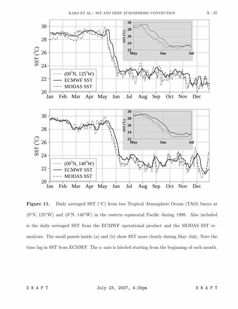
Figure 11. Daily averaged SST (◦C) from two Tropical Atmosphere Ocean (TAO) buoys at

(0◦N, 125◦W) and (0◦N, 140◦W) in the eastern equatorial Pacific during 1998. Also included

is the daily–averaged SST from the ECMWF operational product and the MODAS SST re–

analyses. The small panels inside (a) and (b) show SST more clearly during May–July. Note the

time lag in SST from ECMWF. The x–axis is labeled starting from the beginning of each month.



Figure 12. (a) Monthly mean SST anomaly fields (◦C) from MODAS and HYCOM in the

tropical Pacific just before, during and after the 1998 transition period from El Nino to La

Nina between 20◦S and 20◦N as in Figure 9. (b) Statistics between HYCOM and MODAS SST

calculated using actual SST and SST anomalies, both of which span 1993–2003.



98Jan Feb Mar Apr May Jun Jul Aug Sep Oct Nov Dec

20

22

24

26

28

30

SST

(o C

)

(00oN, 140

oW)

HYCOM SST


50

100

150

200

250

300

Shor

twav

e R

adia

tion

(W m

−2 )

(00oN, 140

oW)

ECMWF


−4

−2

0

2

4

Diff

eren

ce (o C

)

HYCOM−TAO


−200

−100

0

100

200

Diff

eren

ce (

W m

−2 )

ECMWF−TAO

Figure 13. Time series of daily averaged SST (◦C) (from the TAO buoy and HYCOM)

and net shortwave radiation (W m−2) at the sea surface (from the TAO buoy and ECMWF) at

(0◦N 140◦W), along with their differences. Note that the TAO buoy measures shortwave radiation

above the sea surface, and it is multiplied by 0.94 (albedo of sea water) to be consistent with the

shortwave radiation from ECMWF. A 7–day running average is applied to the daily shortwave

radiation time series for illustration purposes. The annual mean of shortwave radiation from

TAO (ECMWF) is 233 (231) W m−2 but note that there are obvious differences between the two

on monthly time scales. Differences in shortwave radiation between the TAO buoy and ECMWF

can even be >≈ 150 W m2 on daily time scales The difference was close to ≈ 200 W m−2 during

mid–May when the 1998 transition was in progress.


Documents

An Eddy–Resolving Ocean Model for the Paciﬁc Ocean: Part 1 ...hycom.rsmas.miami.edu/publications/kara/kara_pacific_part1.pdf · 42 1997–1998 event, ... (air temperature and