An Econometric Analysis of Emission Trading Allowances · An Econometric Analysis of Emission Trading Allowances M. Paolella L. Taschini Swiss Banking Institute University of Zurich,

An EconometricAnalysis of EmissionTrading Allowances

M. Paolella L. TaschiniSwiss Banking

InstituteUniversity of Zurich,

Switzerland

Definition

Motivation

Contribution

Results

SO2 Stylized facts

Zero Excess

Econometric Approach

Unconditional Model

Conditional Model

Stable-MixtureGARCH

Summary of CO2

An Econometric Analysis of EmissionTrading Allowances

M. Paolella L. TaschiniSwiss Banking InstituteUniversity of Zurich,

Switzerland

November 2006




Switzerland

Definition

Motivation

Contribution

Results

SO2 Stylized facts

Zero Excess


Unconditional Model

Conditional Model

Stable-MixtureGARCH

Summary of CO2




Switzerland

Definition

Motivation

Contribution

Results

SO2 Stylized facts

Zero Excess


Unconditional Model

Conditional Model

Stable-MixtureGARCH

Summary of CO2




Switzerland

Definition

Motivation

Contribution

Results

SO2 Stylized facts

Zero Excess


Unconditional Model

Conditional Model

Stable-MixtureGARCH

Summary of CO2




Switzerland

Definition

Motivation

Contribution

Results

SO2 Stylized facts

Zero Excess


Unconditional Model

Conditional Model

Stable-MixtureGARCH

Summary of CO2




Switzerland

Definition

Motivation

Contribution

Results

SO2 Stylized facts

Zero Excess


Unconditional Model

Conditional Model

Stable-MixtureGARCH

Summary of CO2




Switzerland

Definition

Motivation

Contribution

Results

SO2 Stylized facts

Zero Excess


Unconditional Model

Conditional Model

Stable-MixtureGARCH

Summary of CO2

Definition of Tradable Permits

Tradable permits are a cost-efficient, market-driven approach forreducing GHG.

They are tradable allocation entitled by a government to anindividual firm to emit a specific amount of a substance over aspecified interval of time.

They enlists market forces in the quest for cost–effective pollutioncontrol and encouraging technological progress.

Tradable emission permits programs are being adopted byenvironmental regulators in applications ranging from

I local and regional (US-CAAA Title IV)

I global scale (EU-ETS and from 2008 the Kyoto Protocol)




Switzerland

Definition

Motivation

Contribution

Results

SO2 Stylized facts

Zero Excess


Unconditional Model

Conditional Model

Stable-MixtureGARCH

Summary of CO2

Motivation

Emission Allowances influence:

I Commodity markets and energy market;

I Business decisions begin to be made with the price of carbonas a criterion;

I Firms stock value.

Emission Allowances market:

I high volatility and market crash;

I market is working.




Switzerland

Definition

Motivation

Contribution

Results

SO2 Stylized facts

Zero Excess


Unconditional Model

Conditional Model

Stable-MixtureGARCH

Summary of CO2

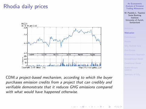
Rhodia daily prices

CDM:a project-based mechanism, according to which the buyerpurchases emission credits from a project that can credibly andverifiable demonstrate that it reduces GHG emissions comparedwith what would have happened otherwise.




Switzerland

Definition

Motivation

Contribution

Results

SO2 Stylized facts

Zero Excess


Unconditional Model

Conditional Model

Stable-MixtureGARCH

Summary of CO2

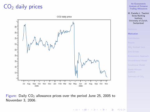
CO2 daily prices

CO2 daily price

Jul Aug Sep Oct Nov Dec Jan Feb Mar Apr May Jun Jul Aug Sep Oct Nov2005 2006

1214

1618

2022

2426

28

Figure: Daily CO2 allowance prices over the period June 25, 2005 toNovember 3, 2006.




Switzerland

Definition

Motivation

Contribution

Results

SO2 Stylized facts

Zero Excess


Unconditional Model

Conditional Model

Stable-MixtureGARCH

Summary of CO2

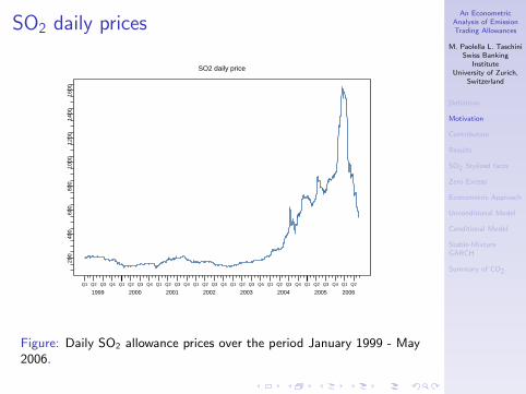
SO2 daily prices

SO2 daily price

Q1 Q2 Q3 Q4 Q1 Q2 Q3 Q4 Q1 Q2 Q3 Q4 Q1 Q2 Q3 Q4 Q1 Q2 Q3 Q4 Q1 Q2 Q3 Q4 Q1 Q2 Q3 Q4 Q1 Q2

1999 2000 2001 2002 2003 2004 2005 2006

200

400

600

800

1000

1200

1400

1600

Figure: Daily SO2 allowance prices over the period January 1999 - May2006.




Switzerland

Definition

Motivation

Contribution

Results

SO2 Stylized facts

Zero Excess


Unconditional Model

Conditional Model

Stable-MixtureGARCH

Summary of CO2

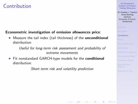
Contribution

Econometric investigation of emission allowances price:

I Measure the tail index (tail thickness) of the unconditionaldistribution:

Useful for long-term risk assessment and probability ofextreme movements

I Fit nonstandard GARCH-type models for the conditionaldistribution:

Short term risk and volatility prediction




Switzerland

Definition

Motivation

Contribution

Results

SO2 Stylized facts

Zero Excess


Unconditional Model

Conditional Model

Stable-MixtureGARCH

Summary of CO2

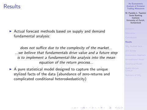
Results

I Actual forecast methods based on supply and demandfundamental analysis:

does not suffice due to the complexity of the market......we believe that fundamentals drive value and a future stepis to implement a fundamental-like analysis into the mean

equation of the return process...

I A pure statistical model designed to capture the uniquestylized facts of the data (abundance of zero-returns andcomplicated conditional heteroskedasticity)




Switzerland

Definition

Motivation

Contribution

Results

SO2 Stylized facts

Zero Excess


Unconditional Model

Conditional Model

Stable-MixtureGARCH

Summary of CO2

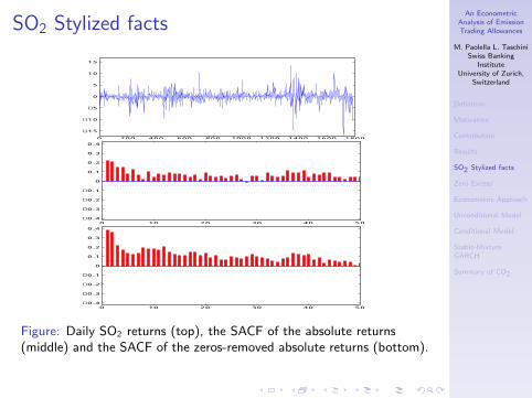
SO2 Stylized facts

0 200 400 600 800 1000 1200 1400 1600 1800

−15

−10

−5

0

5

10

15

0 10 20 30 40 50−0.4

−0.3

−0.2

−0.1

0

0.1

0.2

0.3

0.4

0 10 20 30 40 50−0.4

−0.3

−0.2

−0.1

0

0.1

0.2

0.3

0.4

Figure: Daily SO2 returns (top), the SACF of the absolute returns(middle) and the SACF of the zeros-removed absolute returns (bottom).




Switzerland

Definition

Motivation

Contribution

Results

SO2 Stylized facts

Zero Excess


Unconditional Model

Conditional Model

Stable-MixtureGARCH

Summary of CO2

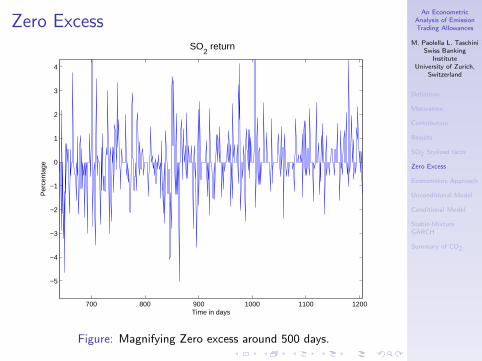
Zero Excess

700 800 900 1000 1100 1200

−5

−4

−3

−2

−1

0

1

2

3

4

Time in days

Per

cent

age

SO2 return

Figure: Magnifying Zero excess around 500 days.




Switzerland

Definition

Motivation

Contribution

Results

SO2 Stylized facts

Zero Excess


Unconditional Model

Conditional Model

Stable-MixtureGARCH

Summary of CO2

Unconditional Distributional Fit: SαSI Large number of zeros precludes use of typical fat-tailed

distributions (t, hyperbolic, stable, etc) because the centerwill be too peaked, forcing the tails to be unnecessarily thick.

I Otherwise, the stable Paretian would be a great candidatedistribution (GCLT, closed under summation, good fit tofinancial returns data, easy VaR approximations)

I The downside is its computation: For the symmetric stable,the characteristic function is

ϕX (t;α) = E[exp{itX}

]= exp {− |t|α} , 0 < α ≤ 2.

and the usual inversion formula reduces to:

fX (x) =1

π

∫ ∞

0

cos (tx) e−tα

dt.

I We use the FFT and linear interpolation to speed up.

I Except for the normal (α = 2) case, the α-stable distributionhas infinite variance. For α ≤ 1, its tails are so heavy thateven the mean does not exist.




Switzerland

Definition

Motivation

Contribution

Results

SO2 Stylized facts

Zero Excess


Unconditional Model

Conditional Model

Stable-MixtureGARCH

Summary of CO2

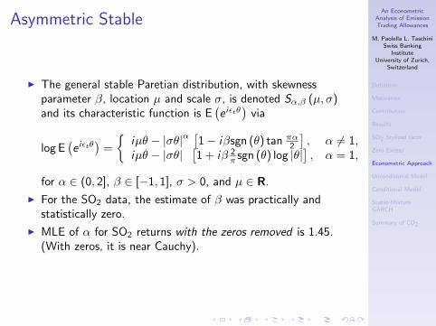
Asymmetric Stable

I The general stable Paretian distribution, with skewnessparameter β, location µ and scale σ, is denoted Sα,β (µ, σ)and its characteristic function is E

(e iεtθ

)via

log E(e iεtθ

)=

{iµθ − |σθ|α

[1− iβsgn (θ) tan πα

2

], α 6= 1,

iµθ − |σθ|[1 + iβ 2

π sgn (θ) log |θ|], α = 1,

for α ∈ (0, 2], β ∈ [−1, 1], σ > 0, and µ ∈ R.

I For the SO2 data, the estimate of β was practically andstatistically zero.

I MLE of α for SO2 returns with the zeros removed is 1.45.(With zeros, it is near Cauchy).




Switzerland

Definition

Motivation

Contribution

Results

SO2 Stylized facts

Zero Excess


Unconditional Model

Conditional Model

Stable-MixtureGARCH

Summary of CO2

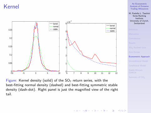
Kernel

−10 −5 0 5 100

0.05

0.1

0.15

0.2

0.25

kernelnormalstable

6 7 8 9 10 11 12 130

1

2

3

4

5

6x 10

−3

kernelnormalstable

Figure: Kernel density (solid) of the SO2 return series, with thebest-fitting normal density (dashed) and best-fitting symmetric stabledensity (dash-dot). Right panel is just the magnified view of the righttail.




Switzerland

Definition

Motivation

Contribution

Results

SO2 Stylized facts

Zero Excess


Unconditional Model

Conditional Model

Stable-MixtureGARCH

Summary of CO2

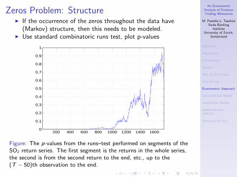
Zeros Problem: StructureI If the occurrence of the zeros throughout the data have

(Markov) structure, then this needs to be modeled.I Use standard combinatoric runs test, plot p-values

200 400 600 800 1000 1200 1400 16000

0.1

0.2

0.3

0.4

0.5

0.6

0.7

0.8

0.9

1

Figure: The p-values from the runs–test performed on segments of theSO2 return series. The first segment is the returns in the whole series,the second is from the second return to the end, etc., up to the(T − 50)th observation to the end.




Switzerland

Definition

Motivation

Contribution

Results

SO2 Stylized facts

Zero Excess


Unconditional Model

Conditional Model

Stable-MixtureGARCH

Summary of CO2

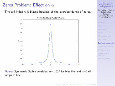
Zeros Problem: Effect on α

The tail index α is biased because of the overabundance of zeros.

−15 −10 −5 0 5 10 150

0.05

0.1

0.15

0.2

0.25

0.3

0.35

0.4

0.45

0.5 Symmetric Stable Paretian Density

x

pdf

Figure: Symmetric Stable densities: α=1.027 for blue line and α=1.64for green line.




Switzerland

Definition

Motivation

Contribution

Results

SO2 Stylized facts

Zero Excess


Unconditional Model

Conditional Model

Stable-MixtureGARCH

Summary of CO2

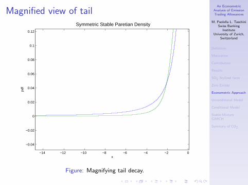
Magnified view of tail

−14 −12 −10 −8 −6 −4 −2 0

−0.04

−0.02

0

0.02

0.04

0.06

0.08

0.1

0.12

Symmetric Stable Paretian Density

x

pdf

Figure: Magnifying tail decay.




Switzerland

Definition

Motivation

Contribution

Results

SO2 Stylized facts

Zero Excess


Unconditional Model

Conditional Model

Stable-MixtureGARCH

Summary of CO2

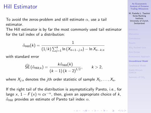
Hill Estimator

To avoid the zeros-problem and still estimate α, use a tailestimator.The Hill estimator is by far the most commonly used tail estimatorfor the tail index of a distribution:

αHill(k) =1

(1/k)∑k

j=1 ln (Xn+1−j :n)− lnXn−k:n

with standard error

SE (αHill;k) =kαHill(k)

(k − 1) (k − 2)1/2, k > 2,

where Xj :n denotes the jth order statistic of sample X1, . . . ,Xn.

If the right tail of the distribution is asymptotically Pareto, i.e., forlarge x , 1− F (x) ≈ cx−α, then, given an appropriate choice of k,αHill provides an estimate of Pareto tail index α.




Switzerland

Definition

Motivation

Contribution

Results

SO2 Stylized facts

Zero Excess


Unconditional Model

Conditional Model

Stable-MixtureGARCH

Summary of CO2

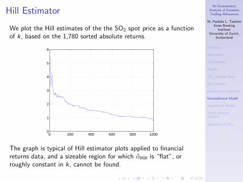
Hill Estimator

We plot the Hill estimates of the the SO2 spot price as a functionof k, based on the 1,780 sorted absolute returns.

0 200 400 600 800 10000

1

2

3

4

5

6

The graph is typical of Hill estimator plots applied to financialreturns data, and a sizeable region for which αHill is “flat”, orroughly constant in k, cannot be found.




Switzerland

Definition

Motivation

Contribution

Results

SO2 Stylized facts

Zero Excess


Unconditional Model

Conditional Model

Stable-MixtureGARCH

Summary of CO2

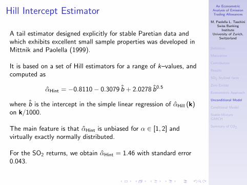
Hill Intercept Estimator

A tail estimator designed explicitly for stable Paretian data andwhich exhibits excellent small sample properties was developed inMittnik and Paolella (1999).

It is based on a set of Hill estimators for a range of k–values, andcomputed as

αHint = −0.8110− 0.3079 b + 2.0278 b0.5

where b is the intercept in the simple linear regression of αHill (k)on k/1000.

The main feature is that αHint is unbiased for α ∈ [1, 2] andvirtually exactly normally distributed.

For the SO2 returns, we obtain αHint = 1.46 with standard error0.043.




Switzerland

Definition

Motivation

Contribution

Results

SO2 Stylized facts

Zero Excess


Unconditional Model

Conditional Model

Stable-MixtureGARCH

Summary of CO2

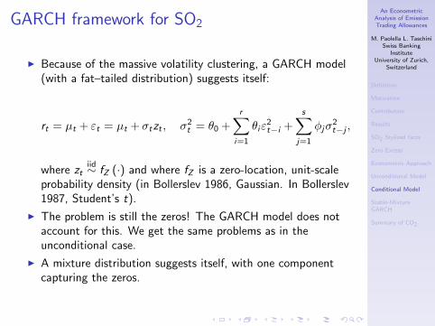
GARCH framework for SO2

I Because of the massive volatility clustering, a GARCH model(with a fat–tailed distribution) suggests itself:

rt = µt + εt = µt + σtzt , σ2t = θ0 +

r∑i=1

θiε2t−i +

s∑j=1

φjσ2t−j ,

where ztiid∼ fZ (·) and where fZ is a zero-location, unit-scale

probability density (in Bollerslev 1986, Gaussian. In Bollerslev1987, Student’s t).

I The problem is still the zeros! The GARCH model does notaccount for this. We get the same problems as in theunconditional case.

I A mixture distribution suggests itself, with one componentcapturing the zeros.




Switzerland

Definition

Motivation

Contribution

Results

SO2 Stylized facts

Zero Excess


Unconditional Model

Conditional Model

Stable-MixtureGARCH

Summary of CO2

Mixture Models

{εt} is generated by an n–component Mixed Normal GARCH(r , s)process, if the conditional distribution of εt is an n–componentmixed normal with zero mean, i.e.,

εt |Ft−1 ∼MN(ω,µ,σ2

t

), (1)

and the mixed normal density is given by

fMN(y ;ω,µ,σ2

)=

n∑j=1

ωjφ(y ;µj , σ

2jt

), (2)

φ is the normal pdf, ωj ∈ (0, 1) with∑n

j=1 ωj = 1 and, to ensure

zero mean, µn = −∑n−1

j=1 (ωj/ωn) µj .The n x 1 component variances evolves according to aGARCH–like structure

σ(2)t = γ0 +

r∑i=1

γ iε2t−i +

s∑j=1

Ψjσ(2)t−j , (3)




Switzerland

Definition

Motivation

Contribution

Results

SO2 Stylized facts

Zero Excess


Unconditional Model

Conditional Model

Stable-MixtureGARCH

Summary of CO2

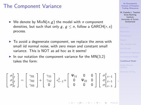
The Component Variance

I We denote by MixN(n, g) the model with n componentdensities, but such that only g , g ≤ n, follow a GARCH(r , s)process.

I To avoid a degenerate component, we replace the zeros withsmall iid normal noise, with zero mean and constant smallvariance. This is NOT as ad hoc as it seems!

I In our notation the component variance for the MN(3,2)takes the form:

σ21t

σ22t

σ23t

=

γ01

γ02

γ03

+

γ11

γ12

0

ε2t−1+

Ψ11 0 00 Ψ22 00 0 0

σ21,t−1

σ22,t−1

σ23,t−1

.




Switzerland

Definition

Motivation

Contribution

Results

SO2 Stylized facts

Zero Excess


Unconditional Model

Conditional Model

Stable-MixtureGARCH

Summary of CO2

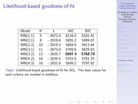
Likelihood-based goodness-of-fit

Model K L AIC BICMN(1,1) 5 −4072.0 8134.0 8181.42MN(2,1) 8 −2919.6 5855.2 5899.07MN(2,2) 10 −2919.3 5858.6 5913.44MN(3,1) 11 −2873.8 5769.6 5829.93MN(3,2) 13 −2835.7 5697.4 5768.70MN(4,2) 16 −2834.5 5701.0 5781.75MN(4,3) 18 −2831.6 5699.2 5797.92

Table: Likelihood-based goodness-of-fit for SO2. The best values foreach criteria are marked in boldface.




Switzerland

Definition

Motivation

Contribution

Results

SO2 Stylized facts

Zero Excess


Unconditional Model

Conditional Model

Stable-MixtureGARCH

Summary of CO2

Empirical Results

Param MN(2,1) MN(3,1) MN(3,2)a0 0.046 0.040 0.041a1 0.000 0.000 0.000

γ01 0.137 0.157 0.621γ11 0.243 0.235 0.427Ψ11 0.797 0.867 0.846ω1 0.709 0.440 0.165µ1 0.019 0.012 −0.001

γ02 0.001 0.505 0.121γ12 - - 0.212Ψ22 - - 0.649ω2 0.290 0.334 0.595µ2 −0.047 0.019 0.001

γ03 - 0.012 0.013γ13 - - -Ψ33 - - -ω3 - 0.226 0.239µ3 - −0.046 −0.045

Table: Maximum likelihood parameter estimates of the mixed normalGARCH models for the SO2 allowances price return 1999-2006.




Switzerland

Definition

Motivation

Contribution

Results

SO2 Stylized facts

Zero Excess


Unconditional Model

Conditional Model

Stable-MixtureGARCH

Summary of CO2

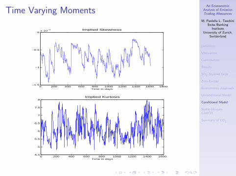
Time Varying Moments

0 200 400 600 800 1000 1200 1400 1600 1800−1.5

−1

−0.5

0x 10

−3

Time in days

Implied Skewness

0 200 400 600 800 1000 1200 1400 16004.5

5

5.5

6

6.5

7

7.5

8

Time in days

Implied Kurtosis




Switzerland

Definition

Motivation

Contribution

Results

SO2 Stylized facts

Zero Excess


Unconditional Model

Conditional Model

Stable-MixtureGARCH

Summary of CO2

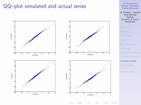
QQ–plot simulated and actual series

−15 −10 −5 0 5 10 15−15

−10

−5

0

5

10

15

X Quantiles

Y Q

uant

iles

−15 −10 −5 0 5 10 15−15

−10

−5

0

5

10

15

X Quantiles

Y Q

uant

iles

−15 −10 −5 0 5 10 15−15

−10

−5

0

5

10

15

X Quantiles

Y Q

uant

iles

−15 −10 −5 0 5 10 15−15

−10

−5

0

5

10

15

20

X Quantiles

Y Q

uant

iles




Switzerland

Definition

Motivation

Contribution

Results

SO2 Stylized facts

Zero Excess


Unconditional Model

Conditional Model

Stable-MixtureGARCH

Summary of CO2

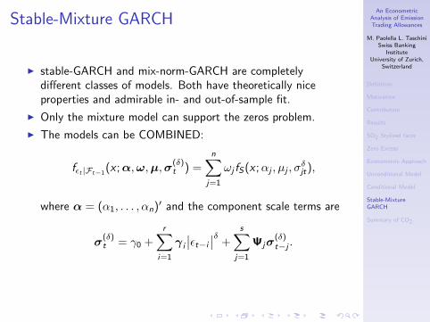
Stable-Mixture GARCH

I stable-GARCH and mix-norm-GARCH are completelydifferent classes of models. Both have theoretically niceproperties and admirable in- and out-of-sample fit.

I Only the mixture model can support the zeros problem.

I The models can be COMBINED:

fεt |Ft−1(x ;α,ω,µ,σ

(δ)t ) =

n∑j=1

ωj fS(x ;αj , µj , σδjt),

where α = (α1, . . . , αn)′ and the component scale terms are

σ(δ)t = γ0 +

r∑i=1

γ i

∣∣εt−i

∣∣δ +s∑

j=1

Ψjσ(δ)t−j .




Switzerland

Definition

Motivation

Contribution

Results

SO2 Stylized facts

Zero Excess


Unconditional Model

Conditional Model

Stable-MixtureGARCH

Summary of CO2

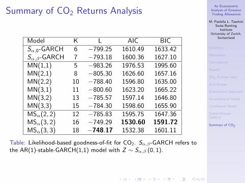
Summary of CO2 Returns Analysis

I Only 337 returns.

I The Hint estimate of the unconditional tail index is1.25(0.091), and removing the single massive negative returngives 1.304(0.092).

I For the normal-mixture models, MN(3,3) and MN(2,2) arenearly as good, according to AIC.

I The best model, by far, is the stable-mixture-GARCH,according to all criteria, despite the large number ofparameters and the small sample size.




Switzerland

Definition

Motivation

Contribution

Results

SO2 Stylized facts

Zero Excess


Unconditional Model

Conditional Model

Stable-MixtureGARCH

Summary of CO2

Summary of CO2 Returns Analysis

Model K L AIC BICSα,0-GARCH 6 −799.25 1610.49 1633.42Sα,β-GARCH 7 −793.18 1600.36 1627.10MN(1,1) 5 −983.26 1976.53 1995.60MN(2,1) 8 −805.30 1626.60 1657.16MN(2,2) 10 −788.40 1596.80 1635.00MN(3,1) 11 −800.60 1623.20 1665.22MN(3,2) 13 −785.57 1597.14 1646.80MN(3,3) 15 −784.30 1598.60 1655.90MSα(2, 2) 12 −785.83 1595.75 1647.36MSα(3, 2) 16 −749.29 1530.60 1591.72MSα(3, 3) 18 −748.17 1532.38 1601.11

Table: Likelihood-based goodness-of-fit for CO2. Sα,β-GARCH refers tothe AR(1)-stable-GARCH(1,1) model with Z ∼ Sα,β (0, 1).

Documents

An Econometric Analysis of Emission Trading Allowances · An Econometric Analysis of Emission Trading Allowances M. Paolella L. Taschini Swiss Banking Institute University of Zurich,