An Efficient GPU-based Time Domain Solver for the Acoustic Wave EquationRavish Mehraa,1, Nikunj Raghuvanshib, Lauri Saviojac, Ming C. Lina, Dinesh Manochaa

aDepartment of Computer Science, 201 South Columbia Street, University of North Carolina at Chapel Hill, NC 27599-3175 USAbMicrosoft Research, One Microsoft Way, Redmond WA 98052-6399 USA

cDepartment of Computer Science, Aalto University School of Science and Technology, P.O. Box 5400 FIN-02015 HUT Finland

Abstract

An efficient algorithm for time-domain solution of the acoustic wave equation for the purpose of room acoustics is presented.It is based on adaptive rectangular decomposition of the scene and uses analytical solutions within the partitions that rely onspatially invariant speed of sound. This technique is suitable for auralizations and sound field visualizations, even on coarsemeshes approaching the Nyquist limit. It is demonstrated that by carefully mapping all components of the algorithm to matchthe parallel processing capabilities of graphics processors (GPUs), significant improvement in performance is gained compared tothe corresponding CPU-based solver, while maintaining the numerical accuracy. Substantial performance gain over a high-orderfinite-difference time-domain method is observed. Using this technique, a 1 second long simulation can be performed on scenesof air volume 7500 m3 till 1650 Hz within 18 minutes compared to the corresponding CPU-based solver that takes around 5 hoursand a high-order finite-difference time-domain solver that could take up to three weeks on a desktop computer. To the best of theauthors’ knowledge, this is the fastest time-domain solver for modeling the room acoustics of large, complex-shaped 3D scenes thatgenerates accurate results for both auralization and visualization.

Keywords: Time-domain wave equation solver, Room acoustics, GPU-based algorithms.

1. Introduction

Computational methods in room acoustics have been an ac-tive area of research and developed in conjunction with diversefields, such as seismology, geophysics, meteorology, for almosthalf a century. The goal of computational acoustic methods ingames and interactive applications, in room acoustics computa-tion, is auralization: generating audio that, when played, mim-ics the aural experience of actually being in the space. Nev-ertheless, achieving good acoustics in large complex structuresremains a major computational challenge [1]. Since numeri-cal acoustic computations are usually not possible in real-time,especially for frequencies in the kilohertz range, auralizationis usually a two-stage process: precomputation of impulse re-sponses from the space and real-time convolution of the im-pulse responses with dry (i.e. anechoically recorded or synthet-ically generated) source signals. The impulse response com-putation requires an accurate calculation of wave propagationfor modeling the time-varying spatial sound field. Anotherimportant goal in room acoustic modeling is visualization ofthis sound field. The ability to visualize and animate transientacoustic phenomena is extremely helpful in intuitively under-standing physically complex acoustic effects such as diffrac-tion, scattering and interference [2] and forms an effective toolfor educational purposes. In future, it could even be used forpractical engineering applications like noise control and archi-tectural acoustics, by helping engineers to quickly locate thegeometric features responsible for acoustical defects.

1.1. Acoustic wave equationThe physics of room acoustics, as well as many other areas,

is described by the well known time-domain formulation of the

1Author to whom correspondence should be addressed. Electronic mail:ravishm@cs.unc.edu, Phone : +1 919-962-1923, Fax: +1 (919) 962-1799.

wave equation –

∂2 p∂t2 − c2∇2 p = f (x, t) . (1)

The wave equation models sound waves as a time-varying pres-sure field, p (x, t). While the speed of sound in air (denotedc) exhibits slight fluctuations within a room due to variationsin temperature and humidity, we ignore the acoustic effects ofsuch small fluctuations in this paper i.e. we assume uniformmedia. We chose a value of c = 340ms−1 corresponding to dryair at 20 degrees centigrade. Volume sound sources in the sceneare modeled by the forcing field denoted f (x, t) on the righthand side in the Equation 1. The operator ∇2 = ∂2

∂x2 +∂2

∂y2 +∂2

∂z2

is the Laplacian in 3D. The wave equation succinctly captureswave phenomena such as interference and diffraction that areobserved in reality. Both the goals of acoustic auralization andvisualization, can be fulfilled by time-domain solvers for theacoustic wave equation.

1.2. Computational challenges

One of the key challenges in time-domain wave-based acous-tic simulation is the computational and memory requirements ofan accurate solver. Finite difference solvers, in order to main-tain low errors, require the spatial discretization to contain 6−10samples per wavelength for the highest usable frequency of in-terest [3, 4, 5]. Errors manifest themselves as numerical disper-sion, where higher frequencies travel slower on the numericalgrid than lower frequencies, leading to phase errors [5]. Togive a quick example of the resulting requirements, if the entirefrequency range of human hearing needs be simulated (i.e. upto 22 kHz), then the spacing between the nodes would have tobe 1.5 − 2.5 mm. As a result, a cubic meter of acoustic space

Preprint submitted to Applied Acoustics June 22, 2011

needs to be filled with 64− 300 million grid cells, and the com-plexity increases proportionally with the volume of the acousticspace. Due to this, prior numerical solvers for the acoustic waveequation have very high computational demands, especially forbroadband simulations extending into the kilohertz range, re-quiring a cluster of machines for execution. Thus, traditionalroom acoustic simulation systems have largely relied on geo-metric acoustic techniques. But these techniques are accurateonly for higher frequencies and early reflections, and face con-siderable difficulties for modeling wave diffraction effects.

Our formulation is based on the adaptive rectangular decom-position (ARD) technique proposed by Raghuvanshi et al. [6].ARD results in little numerical dispersion error as comparedto finite difference methods, allowing for execution on a verycoarse grid, approaching the Nyquist limit. This leads to sub-stantial speedups [6]. The ARD technique assumes an isotropic,homogeneous, dissipation-free medium. The assumptions ofisotropy and homogeneity are critical for the speedup and ac-curacy of the technique. It has been demonstrated recently thatimpulse responses computed using ARD can be used for per-ceptually plausible auralizations in interactive applications suchas computer games [7]. These reasons, along with the fact that ithas been demonstrated to work for both auralization [7, 8] andvisualization purposes [6], motivated our choice of this tech-nique. For auralization and visualization videos, please check-out the supplementary materials or the link [9].

1.3. GPU computing

Over the last decade, Graphics Processing Units or GPUsor graphics processors have evolved from fixed-function pro-cessors specialized for 3D graphics operations to a fully pro-grammable computing platform for a wide variety of computa-tionally demanding applications. Current GPUs are massivelydata-parallel throughput-oriented many-core processors capa-ble of providing teraFLOPS of computing power and extremelyhigh memory bandwidth compared to a high-end CPU. On theother hand, due to their distinctive and peculiar architecture,developing a fast and efficient algorithm that extracts the maxi-mum performance from the GPU, is a challenging task. Tradi-tional algorithms designed for scalar architectures (e.g. CPU)do not translate naturally to parallel architectures (e.g. GPU).In this paper, we present a fast and efficient parallel algorithmbased on ARD for numerically solving the acoustic wave equa-tion in the time-domain, entirely on the GPU.

1.4. Main results

Our main contribution is the utilization of GPU architecturein combination with an efficient parallel technique, to allow fornumerical wave simulation in the medium to high frequencyrange that was earlier extremely slow on a desktop computer.We exploit different levels of parallelism exhibited by ARD,prevent any host-device data transfer bottleneck in our algo-rithm design and perform a novel computationally optimal rect-angular decomposition, resulting in an extremely fast and effi-cient solver for the wave equation. We demonstrate that it ispossible to effectively parallelize all steps of our simulator on

current GPU architectures and exploit the computational powerof the high number of GPU processors. Running on currentgeneration GPUs, our algorithm can yield a speedup of up to25 times over the optimized CPU-based ARD solver. Our GPU-based solver is more than three orders of magnitude faster com-pared to a high-order CPU-based finite-difference time-domain(FDTD) solver. We show that the performance of our techniquescales linearly with the number of GPU processors. In partic-ular, ours is the first solver that can run a 1 second long band-limited simulation of 1650 Hz for both auralization and visual-ization purposes, on scenes with realistically complex geometryand air volume in the range of 7, 500 m3 within 18 minutes ona desktop computer. The single-threaded optimized CPU-basedARD solver presented by Raghuvanshi et al. [6] takes 4 hours40 minutes and the CPU-based high-order FDTD solver basedupon Sakamoto et al. [4] takes 20 days to run the same simula-tion on a desktop machine2.

2. Related Work

2.1. Numerical solvers for the wave equationAccurate high-frequency wave propagation is a very chal-

lenging computational problem because the smallest wave-length governs the grid resolution of the numerical methodsand the scene can be thousands of wavelengths long in eachdimension. There is a large body of existing work on solv-ing the wave equation developed over the past few decades.These methods may be roughly classified into finite elementmethod (FEM) [10], boundary element method (BEM) [11],finite-difference time-domain (FDTD) [5] and spectral meth-ods [12].

Finite element method (FEM) solves for the pressure field ona volumetric mesh composed of discrete simplical cells. Oneof the strengths of FEM is the capability of using unstructuredmeshes with cells of different shapes, thus allowing the (poten-tially complex) boundary of the domain to be represented withmuch more accuracy. However, “skinny” cells can lead to in-accurate and/or unstable simulations. Generating good qualitymeshes in 3D for arbitrary domains is a tough problem and acentral concern for FEM methods. Boundary element method(BEM) utilizes a boundary integral formulation that assumesa homogeneous medium and expresses field values throughoutthe domain in terms of values only on the boundary. Thus, BEMonly requires a discretization of the boundary of the domain.Unfortunately, the resultant linear system is dense as all the sur-face values interact strongly with all the others. Both FEM andBEM are usually employed mainly for the steady-state wave(Helmholtz) equation, as opposed to the full time-domain waveequation, with FEM applied mainly to interior and BEM to ex-terior scattering problems.

Recent work on the fast multipole accelerated frequency-domain BEM [13] has obtained very promising results, show-ing that an asymptotic performance gain can be achieved for

2We use NVIDIA GTX 480 as the GPU and Intel Xeon X5560 (8M Cache,2.80 GHz) as the CPU.

2

frequency domain solution of acoustic problems, yielding per-formance that scales linearly with the surface area of the scene,instead of its volume, as in FEM/FDTD. The combination ofBEM and Fast Multipole Method (FMM), represented as BEM-FMM, is an attractive research direction, since it would allowhandling acoustic spaces or models that are much larger thanthose handled by the current approaches [13]. Assuming thatfurther research makes BEM-FMM applicable for large, com-plex scenes, applying this frequency-domain method for time-domain acoustics still requires a large number of frequency-domain simulations.

The Finite Difference Time Domain (FDTD) method was ex-plicitly designed for solving the time-domain wave equation byYee [14], although in the context of electromagnetic simula-tion [5]. The FDTD method for room acoustics solves for thetime-dependent pressure field on a Cartesian grid by makingdiscrete approximations of the spatial derivative operators andusing an explicit time-stepping scheme. Assume that the spacehas been discretized into a uniform Cartesian grid with spatialspacing h and the time-step is ∆t. We denote the pressure valuep (ih, jh, kh) at time n∆t by p(n)

i, j,k. In the absence of a superscript,it is assumed to be n . The spatial derivative is approximated infinite-difference approaches by applying a constant linear sten-cil, β, for some chosen integral value of d as –

∇2 p =d∑

l=−d

βl

(pi+l, j,k + pi, j+l,k + pi, j,k+l

)+ O(h2d) (2)

The spatial differentiation error is ϵs = O(h2d). The stencilhas a compact support of 2d + 1. For most FDTD implemen-tations, d = 1, yielding second-order spatial accuracy, withβ = 1

h2 {1,−2, 1}. The same analysis can be applied for the timederivative as well. It is typical in time-domain solvers to usesecond-order accurate time-stepping –

∂2 p∂t2

(n)

=1h2

(p(n+1) − 2p(n) + p(n−1)

)+ O(h2). (3)

Standard von Neumann analysis can be used to show thatthe spatio-temporal errors in FDTD appears as frequency-dependent phase velocity, known as numerical dispersion – aswaves propagate, their shape is gradually destroyed due to lossof phase-coherence. For comparison in this paper, we havechosen a sixth-order accurate solver with d = 3 and β =

1180h2 {2,−27, 270,−490, 270,−27, 2}, since it has smaller nu-merical dispersion error than a second-order accurate scheme.

Recently, FDTD has been applied to medium-sized scenes in3D for room acoustic computations by Sakamoto et al. [3, 4].The authors calculated typical room acoustic parameters andcompared the calculated parameters with the actual measuredvalues in the scene. The implementation can take days of com-putation on a small cluster. A very recent technique proposedby Savioja [15] can allow for real-time auralizations till a usablefrequency of roughly 500 Hz on geometries with large volumeusing the Interpolated Wideband (IWB) FDTD scheme runningon GPUs. The IWB-FDTD scheme [16] uses optimized com-pact stencils for reducing numerical dispersion while keeping

the computational expenditure low. This results in schemes thatcan run on spatial sampling as low as with ARD, thus allow-ing for competitive performance as presented here. However,the results presented in Savioja’s work [15] assume a high nu-merical dispersion threshold of 10%, for reducing computationtimes. Whether this numerical dispersion is tolerable for au-ralization and computation of room acoustic parameters is anopen research problem. Once such thresholds have been es-tablished through listening tests, a direct comparison betweenIWB-FDTD, FDTD based upon work of Sakamoto et al. [4]and ARD, would become possible. For this paper, our compar-isons are restricted to FDTD based upon Sakamoto et al. [4] andARD.

Spectral techniques achieve much higher accuracy thanFEM/BEM/FDTD by expanding the field in terms of globalbasis functions. Typically, the basis set is chosen to be theFourier basis or Chebyshev polynomials [12] as the fast fouriertransform (FFT) can be employed for the basis transformation.The Fourier Pseudo-Spectral Time Domain (PSTD) method is aspectral method proposed by Liu [17] for underwater acousticsas an alternative to FDTD to control its numerical dispersionartifacts. The key difference in PSTD compared to FDTD is toutilize spectral approximations for the spatial derivative [17] –

∇2 p ≈ F −1(−k2F (p)

), k2

i, j,k = 4π2 i2l2x + j2

l2y+

k2

l2z

(4)

where Discrete Fourier Transform is denoted by F . The spatialerror shows geometric convergence ϵs = O(hn),∀n > 0, n ∈ Z.This allows meshes with samples per wavelength approaching2, the Nyquist limit, and still allowing vanishingly small dis-persion errors in the spatial derivative. However, this holdsonly if the pressure field is periodic which is not commonlythe case. Errors in ensuring periodicity appear as wrap-aroundeffects where waves exiting from one end of the domain enterfrom the opposite end. Time update is done using a second-order explicit scheme, as in Equation (3). Therefore, althoughspatial errors are controlled in PSTD, errors due to temporalderivative approximation are still present and are of a similarmagnitude as FDTD.

2.2. Geometric methods for the wave equationIn the limit of infinite frequency, the wave equation reduces

to the geometric approximation – expressing wave propaga-tion as rays of energy quanta. The history of geometric meth-ods for acoustics goes back roughly four decades [18]. Mostpresent-day room acoustics software packages use geometricmethods [19]. Recent work such as AD-FRUSTA [20], edge-diffraction [21], beam tracing [22, 23], are able to acceler-ate these methods using ray and volume tracing. There hasalso been work on accelerating geometric techniques on theGPU [24, 25]

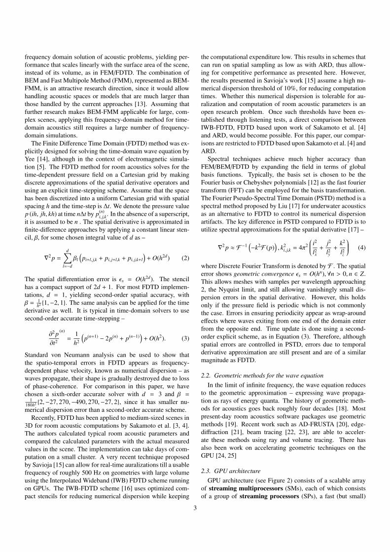
2.3. GPU architectureGPU architecture (see Figure 2) consists of a scalable array

of streaming multiprocessors (SMs), each of which consistsof a group of streaming processors (SPs), a fast (but small)

3

(a) Preprocessing (b) Simulation

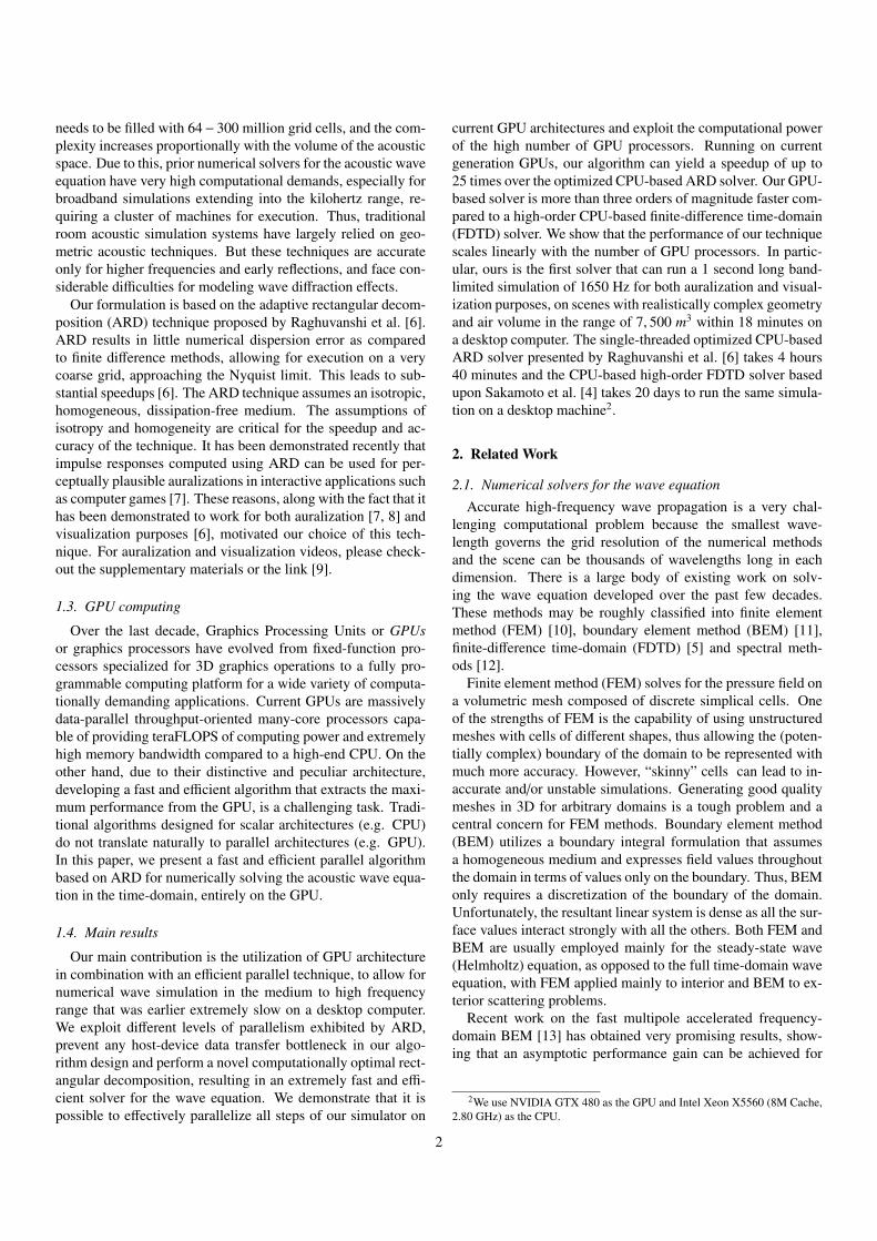
Figure 1: Stages of ARD: a) In the preprocessing stage, the input domain is voxelized into grid cells and adaptively decomposed into rectangular partitions.Artificial interfaces and PML absorbing layers are created between neighboring partitions and on the scene boundary respectively. b) During the simulation stage,we start with the current field and perform interface handling between neighboring partitions to compute forcing terms. We then transform the forcing terms to thecosine spectral basis through DCT. These are then used to update the spectral coefficients to propagate waves within each partition. Lastly, the field is transformedback from spectral to spatial domain using IDCT to yield the updated field.

on-chip shared memory and a SIMT control unit. All the mul-tiprocessors are connected to a large off-chip global memoryvia a interconnection network. In order to effectively solve aproblem on a GPU, first it has to be partitioned into coarse sub-problems that can be solved independently in parallel by blocksof threads. These thread blocks are enumerated and distributedto the available SMs. Each sub-problem is further partitionedin smaller sub-sub-problems that can be solved on SPs coop-eratively in parallel by all the threads within the block. TheSM schedules and executes these threads in groups of paral-lel threads (typically 32) called warps. All the threads of awarp execute a single common instruction at a time. The first orthe second half of a warp is called a half-warp. GPU memoryaccess pattern is based on half-warps. A parallel task is exe-cuted on the GPU by writing functions called kernels which arelaunched by the host-CPU and execute in parallel on the GPU.GPU API provides the ability to create local and global threadbarriers. In a local thread barrier, all the threads in a blockmust wait until every thread of the block has finished executionwhereas in a global thread barrier all the threads on the GPUmust wait until every thread has finished execution. The useof these barriers to synchronize the threads is called as threadsynchronization [26]. For more details on parallel computingon GPUs, please read [27, 28, 29].

Figure 2: The graphics processing unit (GPU) architecture (image c⃝Savioja [15]): Current generation GPUs have many streaming multiproces-sors(SMs), each containing several streaming processors(SPs), a fast on-chipshared memory and a single-instruction multiple-thread (SIMT) control unit.All the multiprocessors are connected to each other and to a larger off-chipglobal memory via a fast interconnection network.

3. Adaptive Rectangular Decomposition

In this section, we give an overview of adaptive rectangu-lar decomposition (ARD) solver [6] and highlight its benefitsover prior solvers for the acoustic wave equation for uniformmedium. Our GPU-based wave equation solver is built uponthe ARD solver.

3.1. ARD Computation Pipeline

ARD has two primary stages, Preprocessing and Simula-tion. In the preprocessing stage, the input scene is voxelizedinto grid cells at grid resolution h determined by the relationh = λmin/s = c/νmaxs where λmin is the minimum simulationwavelength, s is number of samples per wavelength, c is thespeed of sound and νmax is the maximum usable simulation fre-quency3. This is followed by a rectangular decomposition stepin which grid cells generated during voxelization are groupedinto rectangles (see Figure 1(a)). We call these rectangles airpartitions. Partitions created for the perfectly matched layer(PML) absorbing layer are referred to as PML partitions. PMLabsorbing layers are created to model both partially absorbingsurfaces as well as complete absorption in open scenes. Both airand PML partitions have the same grid resolution h. Next, wecreate artificial interfaces between adjacent air-air and air-PMLpartitions. This one-time pre-computation step takes 1-2 min-utes for most scenes. During the simulation stage, the globalacoustic field is computed with a time-marching scheme. Thecomputation at each time-step is as follows (see Figure 1(b)):1. For all interfaces: Interface handling to compute force fwithin each partition (Equation 12).2. For all air partitions:

(a) Discrete Cosine Transform (DCT) of force f to spec-tral domain f (Equation 7).

(b) Mode update for spectral coefficients p (Equation 9).

3By maximum usable frequency of X Hz, we mean that our simulation re-sults have no dispersion error and minimal other numerical errors till X Hz.Therefore, they can be directly used to compute impulse response for auraliza-tion and produce sound field visualization. So νmax = X kHz means that theuseful range of the result is from 0 Hz till X kHz and the excitation is broad-band, containing frequencies from 0 to X kHz

4

(c) Inverse Discrete Cosine Transform (IDCT) of p to pres-sure p (Equation 7).

(d) Normalize pressure p by multiplying it with a normal-ization constant.3. For all PML partitions: Update pressure field.

During step 1, the coupling between adjacent partitions (air-air and air-PML) is computed to produce forcing values. Insteps 2 and 3, these forcing values are used to update the pres-sure fields within the air and PML partitions respectively. Whileair partitions are updated in the spectral domain, transformingto and from spatial domain using IDCT and DCT, PML parti-tions employ a finite-difference implementation of a fictitious,highly dissipative wave equation [30] to perform absorption.DCT and IDCT steps are implemented using a generalized 3DFFT.

3.2. Accuracy and computational aspectsA direct performance comparison of FDTD and ARD for the

same amount of error is difficult since both techniques intro-duce different kinds of errors. Since the final goal in roomacoustics is to auralize the sounds to a human listener, it is natu-ral to set these error tolerances based on their auditory perceiv-ability. This is complicated by the absence of systematic lis-tening tests for perceivable errors with both, FDTD and ARD.However, it is possible to compare them by assuming conser-vatively low errors with both the techniques. We briefly discusshow we set the parameters in both techniques for keeping theerrors conservatively low and then present a theoretical com-parison to motivate why ARD is more compute and memoryefficient than FDTD.

In recent work, Sakamoto et al. [4] show that FDTD cal-culations of room-acoustic impulse responses on a grid withs = 6 − 10 agree well with measured values on a real hall interms of room acoustic parameters such as reverberation time.Remember that grid size h = λmin/s. This mesh resolutionis also commonly used with the finite difference method ap-plied to electromagnetic wave propagation to control phase er-rors resulting from numerical dispersion [5] . Motivated fromthese applications, we set the mesh resolution conservativelyat s = 10 for FDTD throughout this paper, assuming that thissafely ensures that numerical dispersion errors are inaudible inauralizations. ARD results in fictitious reflection errors at theartificial interfaces. As shown by Raghuvanshi et al. [6], usings = 2.6 with ARD, the fictitious reflection errors can be kept ata low level of −40 dB average over the whole usable frequencyrange by employing a sixth-order finite difference transmissionoperator. This means that for a complex scene with many inter-faces, the global errors stay 40 dB below the level of the ambi-ent sound field, rendering them imperceptible as demonstratedin the auralizations [6, 8, 7]. Therefore, we assume sampling ofs = 2.6 for ARD.

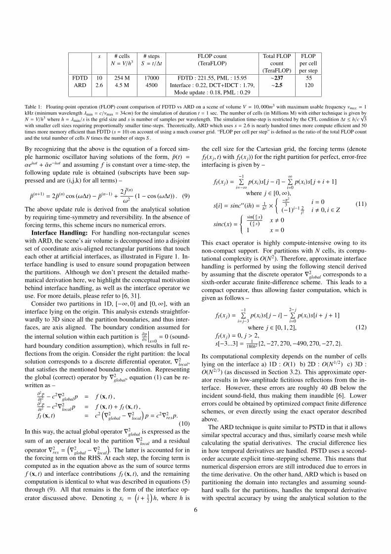
Table 1 shows the performance and memory comparisonof FDTD and ARD. The update cost for sixth-order accurateFDTD in 3D is about 55 FLOP per cell per step including thecost of PML boundary treatment for a stencil width of 7. Thetotal cost for ARD per step can be broken down as: DCT andIDCT (assuming a DCT and IDCT take 2N log2 N FLOP count

each) = 4N log2 N, mode update = 9N, interface handling= (300 × 6N2/3) and PML boundary treatment = (390 × 6N2/3)(the 6N2/3 term approximates the surface area of the scene bythat of a cube with equivalent volume. Due to the cartesiangrid, this estimate is the lower bound of the surface area). PMLboundary treatment cost per cell is the same for both FDTD andARD. As can be seen in the table, theoretically ARD is nearly100 times more compute efficient and 50 times more memoryefficient than FDTD. In practice, the CPU-based ARD is 50−75times faster than FDTD implementation, as discussed in detailin Section 5. Since ARD is highly memory efficient, an orderof magnitude more than FDTD, this makes it possible to per-form simulations on much larger scenes than FDTD withoutoverflowing main memory or GPU memory. GPUs can easilybecome memory-bound, in which case the performance is dic-tated by memory bandwidth rather than the FLOP numbers. Inthese cases as well, ARD, on account of being more memoryefficient, is more suitable for the GPUs.

3.3. Mathematical Background

ARD achieves high accuracy for both spatial and temporalderivatives within rectangular volumes, nearly eliminating nu-merical dispersion. This is done by employing the eigendecom-position for the wave equation on rectangular domains, which,assuming spatially constant speed of sound, can be computedanalytically, incurring no numerical computation or error, asfollows –

∇2Φi, j,k = −k2i, j,kΦi, j,k,

Φi, j,k = cos(π i

lxx)

cos(π j

lyy)

cos(π k

lzz),

k2i, j,k = π2

(i2

l2x+

j2

l2y+ k2

l2z

).

(5)

Note that the eigen-functions, Φi, j,k, coincide with the basisfunctions for the 3D Discrete Cosine Transform. This followsfrom assuming sound-hard boundary conditions for the volume.The result is that to transform to and from the spectral basis,one can leverage memory and compute-efficient Discrete Co-sine Transform (DCT) and inverse Discrete Cosine Transform(iDCT) implementations. The pressure and forcing fields areexpressed in this basis as –

p (x, y, z, t) =∑i, j,k

pi, j,k (t)Φi, j,k (x, y, z) ,

f (x, y, z, t) =∑i, j,k

fi, j,k (t)Φi, j,k (x, y, z) . (6)

The above equations are equivalent to –

pi, j,k(t) = DCT (p (x, y, z, t)),fi, j,k(t) = DCT ( f (x, y, z, t)),p (x, y, z, t) = IDCT (pi, j,k(t)),f (x, y, z, t) = IDCT ( fi, j,k(t)).

(7)

Substituting equation (6) into the wave equation (1) leads toa independent set of Ordinary Differential Equations –

d2 pi, j,k

dt2 + ω2i, j,k pi, j,k = fi, j,k, where ωi, j,k = cki, j,k. (8)

5

s # cells # steps FLOP count Total FLOP FLOPN = V/h3 S = t/∆t (TeraFLOP) count per cell

(TeraFLOP) per stepFDTD 10 254 M 17000 FDTD : 221.55, PML : 15.95 ∼237 55ARD 2.6 4.5 M 4500 Interface : 0.22, DCT+IDCT : 1.79, ∼2.5 120

Mode update : 0.18, PML : 0.29

Table 1: Floating-point operation (FLOP) count comparison of FDTD vs ARD on a scene of volume V = 10, 000m3 with maximum usable frequency νmax = 1kHz (minimum wavelength λmin = c/νmax = 34cm) for the simulation of duration t = 1 sec. The number of cells (in Millions M) with either technique is given byN = V/h3 where h = λmin/s is the grid size and s is number of samples per wavelength. The simulation time-step is restricted by the CFL condition ∆t ≤ h/c

√3

with smaller cell sizes requiring proportionally smaller time-steps. Theoretically, ARD which uses s = 2.6 is nearly hundred times more compute efficient and 50times more memory efficient than FDTD (s = 10) on account of using a much coarser grid. “FLOP per cell per step” is defined as the ratio of the total FLOP countand the total number of cells N times the number of steps S .

By recognizing that the above is the equation of a forced sim-ple harmonic oscillator having solutions of the form, p(t) =αeiωt + αe−iωt and assuming f is constant over a time-step, thefollowing update rule is obtained (subscripts have been sup-pressed and are (i,j,k) for all terms) –

p(n+1) = 2 p(n) cos (ω∆t) − p(n−1) +2 f (n)

ω2 (1 − cos (ω∆t)) . (9)

The above update rule is derived from the analytical solutionby requiring time-symmetry and reversibility. In the absence offorcing terms, this scheme incurs no numerical errors.

Interface Handling: For handling non-rectangular sceneswith ARD, the scene’s air volume is decomposed into a disjointset of coordinate axis-aligned rectangular partitions that toucheach other at artificial interfaces, as illustrated in Figure 1. In-terface handling is used to ensure sound propagation betweenthe partitions. Although we don’t present the detailed mathe-matical derivation here, we highlight the conceptual motivationbehind interface handling, as well as the interface operator weuse. For more details, please refer to [6, 31].

Consider two partitions in 1D, [−∞, 0] and [0,∞], with aninterface lying on the origin. This analysis extends straightfor-wardly to 3D since all the partition boundaries, and thus inter-faces, are axis aligned. The boundary condition assumed forthe internal solution within each partition is ∂p

∂x

∣∣∣∣x=0= 0 (sound-

hard boundary condition assumption), which results in full re-flections from the origin. Consider the right partition: the localsolution corresponds to a discrete differential operator, ∇2

local,that satisfies the mentioned boundary condition. Representingthe global (correct) operator by ∇2

global, equation (1) can be re-written as –

∂2 p∂t2 − c2∇2

global p = f (x, t) ,∂2 p∂t2 − c2∇2

local p = f (x, t) + fI (x, t) ,fI (x, t) = c2

(∇2

global − ∇2local

)p = c2∇2

res p.(10)

In this way, the actual global operator ∇2global is expressed as the

sum of an operator local to the partition ∇2local and a residual

operator ∇2res =

(∇2

global − ∇2local

). The latter is accounted for in

the forcing term on the RHS. At each step, the forcing term iscomputed as in the equation above as the sum of source termsf (x, t) and interface contributions fI (x, t), and the remainingcomputation is identical to what was described in equations (5)through (9). All that remains is the form of the interface op-erator discussed above. Denoting xi =

(i + 1

2

)h, where h is

the cell size for the Cartesian grid, the forcing terms (denotefI(x j, t) with fI(x j)) for the right partition for perfect, error-freeinterfacing is given by –

fI(x j) =−1∑

i=−∞p(xi)s[ j − i] −

∞∑i=0

p(xi)s[ j + i + 1]

where j ∈ [0,∞),

s[i] = sinc′′(ih) = 1h2 ×{ −π2

3 i = 0(−1)i−1 2

i2 i , 0, i ∈ Z

sinc(x) =

sin( πh x)( πh x) x , 0

1 x = 0

(11)

This exact operator is highly compute-intensive owing to itsnon-compact support. For partitions with N cells, its compu-tational complexity is O(N2). Therefore, approximate interfacehandling is performed by using the following stencil derivedby assuming that the discrete operator ∇2

global corresponds to asixth-order accurate finite-difference scheme. This leads to acompact operator, thus allowing faster computation, which isgiven as follows –

fI(x j) =−1∑

i= j−3p(xi)s[ j − i] −

2− j∑i=0

p(xi)s[i + j + 1]

where j ∈ [0, 1, 2],fI(x j) = 0, j > 2,s[−3...3] = 1

180h2 {2,−27, 270,−490, 270,−27, 2}.

(12)

Its computational complexity depends on the number of cellslying on the interface a) 1D : O(1) b) 2D : O(N1/2) c) 3D :O(N2/3) (as discussed in Section 3.2). This approximate oper-ator results in low-amplitude fictitious reflections from the in-terface. However, these errors are roughly 40 dB below theincident sound-field, thus making them inaudible [6]. Lowererrors could be obtained by optimized compact finite differenceschemes, or even directly using the exact operator describedabove.

The ARD technique is quite similar to PSTD in that it allowssimilar spectral accuracy and thus, similarly coarse mesh whilecalculating the spatial derivatives. The crucial difference liesin how temporal derivatives are handled. PSTD uses a second-order accurate explicit time-stepping scheme. This means thatnumerical dispersion errors are still introduced due to errors inthe time derivative. On the other hand, ARD which is based onpartitioning the domain into rectangles and assuming sound-hard walls for the partitions, handles the temporal derivativewith spectral accuracy by using the analytical solution to the

6

wave equation for rectangular spaces. Thus, numerical disper-sion is completely eliminated with ARD for propagation withinrectangular partitions. Some dispersive error is still introducedfor waves propagating across partition interfaces, but this erroris much smaller than with FDTD or even PSTD, where wavesaccumulate dispersive errors of similar magnitude at each time-step.

4. GPU-based acoustic solver

In previous sections, we discussed the computational effi-ciency and mathematical background of ARD. In this section,we describe our parallel GPU-based acoustic wave equationsolver built on top of ARD. We discuss key features of our ap-proach and some of the issues that arise in parallelizing it onmany-core GPU architecture.

4.1. Our GPU approach

Two levels of parallelism. The ARD technique exhibits twolevels of parallelism (a) a coarse-grained and (b) a fine-grained.Coarse grained parallelism is due to the fact that each of the par-titions (air or PML) solves the wave equation independently ofeach other. Therefore, each partition can be solved in parallelat the same time. Fine grained parallelism is achieved becausewithin each partition all the grid cells are independent of eachother with regards to solving the wave equation at a particulartime-step. For solving the wave equation at the current time-step, a grid cell may use p, f , p, f values of its neighboring cellscomputed at previous time-step but is completely independentof their p, f , p, f values at the current time-step. In other words,because ARD uses explicit time-stepping, there is no need forsolving a linear system. Therefore within each partition, allthe grid cells can run in parallel exhibiting fine grained paral-lelism. Our GPU-based acoustic solver exploits both these lev-els of parallelism. We launch as many tasks in parallel as thereare partitions. Each task is responsible for solving the waveequation for a particular partition. Within each task, each gridcell corresponds to a thread and we create as many threads asthe number of grid cells in that partition. All these threads aregrouped into blocks and scheduled by the runtime environmenton the GPU.

Avoiding host-device data transfer bottleneck. The host-device data link between CPU and GPU via PCI express or In-finiband, is a precious resource that has a limited bandwidth.Many prior GPU-based numerical solvers were based uponthe hybrid CPU-GPU design. This design suffers from data-transfer bottleneck as it has to transfer large amounts of databetween host (CPU) and device (GPU) at each simulation step.We have designed our GPU-based solver to ensure that the data-transfer between the CPU-host and GPU-device is minimal. Inour case, we avoid the hybrid CPU-GPU approach and insteadparallelize the entire ARD technique on the GPU. The onlyhost-device data transfer that is required is to store the pressuregrid p after each simulation step. Recent work on interactiveauralization has shown that storing and processing the results

of simulation on a spatial grid subsampled by retaining everyfourth, eighth or sixteenth sample, can be used for convincingauralizations for moving sources and listener, after careful in-terpolation [7]. This results in a memory reduction by a factorof 1/43, 1/83, 1/163 of the original size respectively, resultingin negligible overall cost for transferring the simulation resultsfrom GPU to CPU.

To provide an intuition of host-device data transfer, considera room of air volume 10, 000m3 for which we solve the waveequation at νmax = 2 kHz. We consider a hybrid CPU-GPU sys-tem of Raghuvanshi et al. [8] where only the DCT/IDCT stepsof the technique are parallelized on GPU. In this case, at eachtime-step the grid f is transferred from CPU to GPU for DCT,f is returned back by the GPU, p is transferred from CPU toGPU for IDCT and the final pressure p is returned to the CPU.An important point to note here is that the p, f , p, f grids cannotbe subsampled and transferred in this hybrid CPU-GPU sys-tem because the steps of the algorithm that reside on the CPUand GPU require the values on the complete grid to solve waveequation. Since the size of p, f , p, f is equal to number of gridcells, the total data transfer cost per time-step is 4 x # grid cellsx sizeof(float) = 4V

(sνmax

c

)3x 4 bytes = 4x10000x

(2.6x2000

340

)3x

4 bytes = 145 MB. On the other hand, in our technique since allthe computational steps are performed on the GPU, we do notneed to transfer the p, f , p, f grids to the CPU for the purpose ofthe simulation. The only transfer that is required is of the sub-sampled pressure grid p from GPU to CPU for storage on thedisk, perhaps for auralization later. For visualization applica-tions, one might not need to perform any transfer at all becausethe data is already present on the GPU and can be displayeddirectly to the screen. As explained above, for the purpose ofauralization, the subsampling of pressure grid is usually done ata lower resolution (1/83). Thus our data transfer per time-step= 1/83 x # grid cells x 4 bytes = 3 kB. For such a small size,data-transfer is almost immediate(< 1 msec).

Computationally optimal decomposition. Rectangular de-composition proposed by Raghuvanshi et al. [6] uses a greedyheuristic to decompose the voxelized scene into rectangular par-titions. Specifically, they place a random seed in the scene andtry to find the largest fitting rectangle that can be grown fromthat location. This is repeated until all the free cells of the sceneare exhausted. The cost of DCT and IDCT steps implementedusing FFT depends on the number of grid cells in each parti-tion. FFT operations are known to be extremely efficient if thenumber of grid cells are powers of 2. The proposed heuristicmay produce partitions with irregular number of grid cells (notnecessarily powers of 2) significantly increasing the cost of theDCT and IDCT operations.

We propose a new approach to perform the rectangular de-composition that takes into account the computational expen-diture of FFTs and its efficiency with powers of 2. Specifi-cally, while performing rectangular decomposition, we imposethe constraint that the number of grid cells in each partitionshould be a power of 2. Similar to the original approach, wetry to fill the largest possible rectangle that could fit within theremaining air volume of the scene. But instead of directly using

7

it we shrink its size in each dimension to the nearest power of 2and declare the remaining cells as free. We repeat this step untilall the free cells of the scene are exhausted. This increases theefficiency of the FFT computations and results in a speedup of3 times in the running time of DCT and IDCT steps. For typ-ical scenes, our rectangular decomposition approach produceshigher number (2 − 3 times) of rectangular partitions, but sincethe total number of grid cells in the entire volume of domain re-mains constant (N = V/h3), it does not increase the total FLOPcount except the interface handling step. Since more partitionsresult in larger interface area, the interface handling cost in-creases by 25-30%. But since on the CPU, DCT and IDCTare the most time-consuming steps of the ARD technique com-pared to the cost of interface handling (Figure 5(a) : CPU time),the gain achieved by faster powers-of-two DCT and IDCT faroutweighs this increased interface handling cost.

4.2. Details

Among ARD’s two main stages, the pre-processing is per-formed only once in the beginning and its contribution to thetotal running time is negligible (1− 2 minutes) compared to thecost of the simulation step. Therefore, we keep this stage onthe CPU itself and parallelize the simulation stage on the GPU.Thus, the voxelization and rectangular decomposition is per-formed on the CPU. Once we have the rectangular partitions,we create the pressure p, force f , spectral pressure p and spec-tral force f data-structures on the GPU. The simulation stagehas 6 main steps (see Section 3.1) and each of them is per-formed in sequential order. We now discuss the parallelizationof all these steps on the GPU in detail.

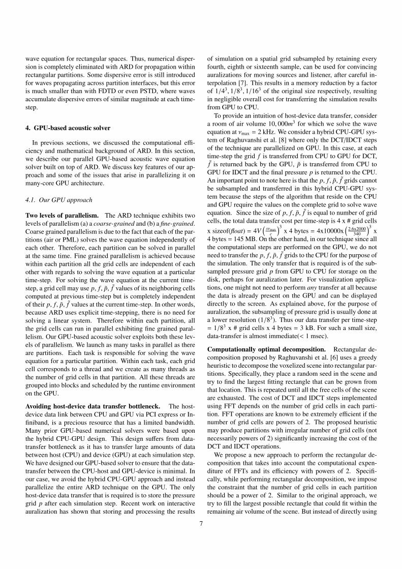
Interface handling. This step is responsible for computingforcing terms f at the artificial interfaces between air-air andair-PML partitions. These forces account for the sound propa-gation between partitions by applying a finite-difference stencilgiven in Equation 12. The overall procedure consists of iter-ating over all interfaces, applying the finite difference stencilsto compute forcing values and additively accumulating them atthe affected cells. This step is data parallel – to compute theforcing term at a cell, only values in its spatial neighborhoodare read. Thus, all interfaces could potentially be processed inparallel as long as there are no collisions and no two interfacesupdate the forcing value at the same cell. This can happen atcorners (as shown below).

Figure 3: (Color online) Interfaces 1 and 2 update forcing values of cells lyingin their neighboring partitions. There is a Concurrent Write (CW) hazard in thehatched corner region (labeled “Collision ”).

Interfaces 1 and 2 both update the forcing values 3-cells deepof their shared partitions. However, for partition P, cells lying

in the hatched region (marked “Collision”) are updated by bothinterfaces 1 and 2. These corner cases need to be addressed toavoid race conditions and concurrent memory writes. The GPUand its runtime environment places the burden of avoiding con-current write (CW) hazards on the programmer. Fortunately,collisions can be avoided completely by using a conceptuallysimple technique. All interfaces are grouped into 3 batches con-sisting of interfaces with their normals in the X, Y and Z direc-tions respectively. Since all partitions are axis-aligned rectan-gles, every interface has to fall into one of these batches. Byprocessing all interfaces within each batch in parallel and sep-arating batches by a synchronization across all threads, all col-lisions in the corners are avoided completely. Our approach ismore general and well-supported on all GPUs.

DCT( f ) . The DCT step converts the force f from the spatialdomain to the spectral domain f . DCTs are efficiently com-puted using FFTs. Typical FFT libraries running on GPU arean order of magnitude faster than optimized CPU implementa-tions [32]. Since DCT and IDCT steps are among the sloweststeps of the ARD technique (see Figure 5(a)), parallelization ofthese steps results in a great improvement in the performanceof the entire technique.

Mode update p . The Mode update step uses the pressureand force in the spectral domain p, f of the previous time-stepto calculate p at the current time-step. This step consists oflinear combinations of p, f terms (see Equation 9) and is highlyparallelizable4.

Pressure normalize p. This step multiplies a constant valueto the pressure p, which is also highly parallelizable.

IDCT( p). This step converts the pressure in the spectral do-main p back to pressure in spatial domain p. Similar to DCTs,the IDCTs are also efficiently computed using FFTs on GPU.

PML absorption layer. The PML absorbing layer is respon-sible for sound wave absorption by the surfaces and walls ofthe 3D environment. It is applied on a 5-10 cell thick partitiondepending on the desired accuracy [30, 6]. We use a 4th orderfinite-difference stencil (5 cell thickness) for PML computation(see Equation 2). Based upon the distance of the grid cell fromthe interface, PML performs different computations for differ-ent grid cells. Due to this, there are a lot of inherent conditionalsin the algorithm. An efficient implementation of PML dependson minimizing the effect of these conditionals, as discussed inthe next section.

4.3. Optimization

The performance of the GPU-based ARD algorithm de-scribed above can be improved by means of following optimiza-tions.

4By highly parallelizable, we mean that there should be no dependence be-tween the threads, each thread has a very local and small memory access patternand all of them can be computed in parallel.

8

Batch processing. Interface handling, DCT, IDCT, Mode up-date and Pressure normalize steps form the main components ofour GPU-based solver, where each step corresponds to a GPU-function called kernel. Kernels are functions that are executedin parallel on the GPU (see Section 2.3). To run these steps onall the partitions and interfaces, one possible way is to launch anew kernel for each individual air partition, PML partition andinterface. In typical scenes, there are thousands of partitionsand interfaces (see Table 2). Since each kernel launch has anassociated overhead, launching thousands of kernels can have adrastic impact on the overall runtime. To avoid this overhead,we group together partitions and interfaces into independentgroups (also called batches) and launch a kernel for each batch.We call this batch processing. Therefore, instead of launchingP + I kernels where P is the number of partitions and I is thenumber of interfaces, we launch as many kernels as there are thenumber of batches. This grouping of partitions into batches de-pends on the number of independent groups that can be formed.If all the partitions are independent, they can grouped into a sin-gle batch. For DCT and IDCT kernels, partitions are groupedinto batches by using the BATCH FFT scheme of the GPU-FFTlibrary [32]. Mode update and Pressure normalize steps have nodependency between different partitions, and are grouped in asingle batch resulting in just one kernel launch each. For PMLstep also, we can group all the PML partitions into a singlebatch and launch a single kernel. But to minimize the effectof conditionals, we launch more than one kernel, as discussedlater. For interface handling, we group the interfaces into 3 sep-arate independent batches as discussed in Section 4.2. A kernellaunch for each batch is followed by a call to synchronize allthe threads.

Maximizing coalesced memory access. The global mem-ory access pattern of the GPU can have a significant impacton its bandwidth. GPU accesses memory in group of threadscalled a half-warp (see Section 2.3). Global memory accessesare most efficient when memory accesses of all the threads ofa half-warp can be coalesced in a single memory access. Ourp, f , p, f data-structures and their memory access patterns forthe Mode update and Pressure normalize kernels are organizedin a way such that each thread of index i accesses these data-structures at position i itself. Thus the memory access patternof a half-warp is perfectly coalesced. DCT and IDCT kernelsbased upon FFT library [32] use memory coalescing as well.Our PML handling kernel for thread i accesses memory at lo-cations α + i where α is constant. This type of access results ina coalesced memory access on current generation GPUs [27].The interface handling step can access p, f from many parti-tions and therefore achieving coalesced memory access for thiskernel is difficult.

Minimizing path divergence . The impact of conditionals(if/else statements) on the performance of a GPU kernel can bevery severe. The PML absorbing layer steps have conditionalsthat are based upon the distance of the grid cells from the inter-face and special cases like outer edges and corners. In our im-plementation, we take specific care in minimizing the effect of

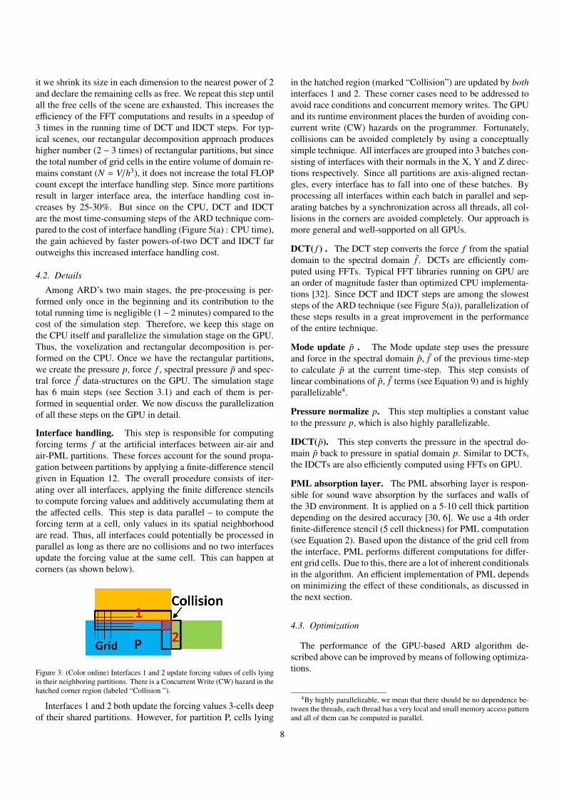
Scene Air/Total νmax # partitions # cellsVolume (m3) Hz (air+pml) (air+pml)

L-shaped room 6998/13520 1875 424+352 (22+5)MCathedral 7381/15120 1650 6130+12110 (16+6)MWalkway 6411/9000 1875 937+882 (20+6)M

Train station 15000/83640 1350 3824+4945 (17+8)MLiving room 5684/7392 1875 3228+4518 (18+5)MSmall room 124/162 7000 3778+5245 (20+5)M

Table 2: “Total volume” is volume of the bounding box of the scene whereas“Air volume” is volume of the air medium in which we perform the simula-tion. νmax is the maximum usable simulation frequency. Number of partitionscounted are generated using our computationally optimal decomposition. Num-ber of pressure values updated at each time-step is equal to the number of gridcells (in millions M).

conditional branching. Instead of launching a single kernel withconditional branching, we launch separate small kernels corre-sponding to different execution paths of the code. The numberof different execution paths is limited and can be reformatted in2-3 unique paths. Thus, the increase in the number of kernellaunches is minimal (2 or 3). These additional kernel launchesdo not adversely impact the performance.

5. Implementation and Results

The original CPU-based ARD solver used a serial version ofFFTW library for computing DCT and IDCT steps. The CPUcode uses two separate threads - one for air partitions and otherfor PML partitions, and performs both these computations inparallel. For simplicity of comparison with our GPU-based im-plementation, we measure the sequential performance of theCPU-based solver by using only a single thread. The CPU-based ARD code has been demonstrated to be sufficiently accu-rate in single precision [8, 6]. Since the calculations performedin our GPU-based approach are the same as the CPU-based ap-proach, the results of the GPU-based solver match the CPU-based solver up to single-precision accuracy. We implementedour GPU-based wave equation solver using NVIDIA’s parallelcomputing API, CUDA 3.0 with minimum compute capability1.0. The following compiler and optimization options are usedfor our GPU code –

nvcc CUDA v3.0 : Maximize Speed (/O2).

Our DCT and IDCT kernels are based upon the FFT librarydeveloped by Govindaraju et al. [32]. We use CUDA routinecudaThreadSynchronize() for synchronizing threads.

We compare our GPU-based acoustic wave equation solverwith the well-optimized CPU implementation provided by theauthors of ARD [6]. We use NVIDIA Geforce GTX 480 graph-ics card with a core clock speed of 700 MHz, graphics memoryof 1.5 GB with 480 CUDA processors (also called cores). CPUtimings are reported for an Intel Xeon X5560 (8M Cache, 2.80GHz) machine. We employ only a single core for the CPU-based implementation. Timings are reported by running thesimulation over 100 time-steps and taking the average. We use5 benchmark scenes varying in both size and complexity (see

9

(a) (b)

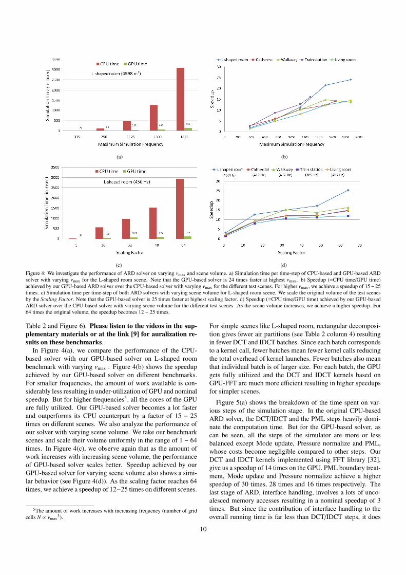
(c) (d)Figure 4: We investigate the performance of ARD solver on varying νmax and scene volume. a) Simulation time per time-step of CPU-based and GPU-based ARDsolver with varying νmax for the L-shaped room scene. Note that the GPU-based solver is 24 times faster at highest νmax. b) Speedup (=CPU time/GPU time)achieved by our GPU-based ARD solver over the CPU-based solver with varying νmax for the different test scenes. For higher νmax, we achieve a speedup of 15−25times. c) Simulation time per time-step of both ARD solvers with varying scene volume for L-shaped room scene. We scale the original volume of the test scenesby the Scaling Factor. Note that the GPU-based solver is 25 times faster at highest scaling factor. d) Speedup (=CPU time/GPU time) achieved by our GPU-basedARD solver over the CPU-based solver with varying scene volume for the different test scenes. As the scene volume increases, we achieve a higher speedup. For64 times the original volume, the speedup becomes 12 − 25 times.

Table 2 and Figure 6). Please listen to the videos in the sup-plementary materials or at the link [9] for auralization re-sults on these benchmarks.

In Figure 4(a), we compare the performance of the CPU-based solver with our GPU-based solver on L-shaped roombenchmark with varying νmax . Figure 4(b) shows the speedupachieved by our GPU-based solver on different benchmarks.For smaller frequencies, the amount of work available is con-siderably less resulting in under-utilization of GPU and nominalspeedup. But for higher frequencies5, all the cores of the GPUare fully utilized. Our GPU-based solver becomes a lot fasterand outperforms its CPU counterpart by a factor of 15 − 25times on different scenes. We also analyze the performance ofour solver with varying scene volume. We take our benchmarkscenes and scale their volume uniformly in the range of 1 − 64times. In Figure 4(c), we observe again that as the amount ofwork increases with increasing scene volume, the performanceof GPU-based solver scales better. Speedup achieved by ourGPU-based solver for varying scene volume also shows a simi-lar behavior (see Figure 4(d)). As the scaling factor reaches 64times, we achieve a speedup of 12−25 times on different scenes.

5The amount of work increases with increasing frequency (number of gridcells N ∝ νmax

3).

For simple scenes like L-shaped room, rectangular decomposi-tion gives fewer air partitions (see Table 2 column 4) resultingin fewer DCT and IDCT batches. Since each batch correspondsto a kernel call, fewer batches mean fewer kernel calls reducingthe total overhead of kernel launches. Fewer batches also meanthat individual batch is of larger size. For each batch, the GPUgets fully utiliized and the DCT and IDCT kernels based onGPU-FFT are much more efficient resulting in higher speedupsfor simpler scenes.

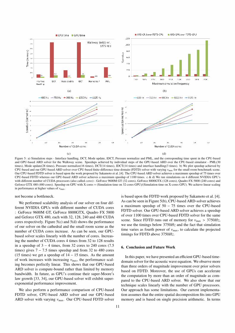
Figure 5(a) shows the breakdown of the time spent on var-ious steps of the simulation stage. In the original CPU-basedARD solver, the DCT/IDCT and the PML steps heavily domi-nate the computation time. But for the GPU-based solver, ascan be seen, all the steps of the simulator are more or lessbalanced except Mode update, Pressure normalize and PML,whose costs become negligible compared to other steps. OurDCT and IDCT kernels implemented using FFT library [32],give us a speedup of 14 times on the GPU. PML boundary treat-ment, Mode update and Pressure normalize achieve a higherspeedup of 30 times, 28 times and 16 times respectively. Thelast stage of ARD, interface handling, involves a lots of unco-alesced memory accesses resulting in a nominal speedup of 3times. But since the contribution of interface handling to theoverall running time is far less than DCT/IDCT steps, it does

10

(a) (b)

(c) (d)Figure 5: a) Simulation steps - Interface handling, DCT, Mode update, IDCT, Pressure normalize and PML, and the corresponding time spent in the CPU-basedand GPU-based ARD solver for the Walkway scene. Speedups achieved by individual steps of the GPU-based ARD over the CPU-based simulator - PML(30times), Mode update(28 times), Pressure normalize(16 times), DCT(14 times), IDCT(14 times) and interface handling(3 times). b) We plot speedup achieved byCPU-based and our GPU-based ARD solver over CPU-based finite-difference time-domain (FDTD) solver with varying νmax for the small room benchmark scene.Our CPU-based FDTD solver is based upon the work proposed by Sakamoto et al. [4]. The CPU-based ARD solver achieves a maximum speedup of 75 times overCPU-based FDTD whereas our GPU-based ARD solver achieves a maximum speedup of 1100 times. c & d) We run simulations on 4 different NVIDIA GPU’swith different number of CUDA processors (also called cores) - GeForce 9600M GT (32 cores), GeForce 8800GTX (128 cores), Quadro FX 5800 (240 cores) andGeforce GTX 480 (480 cores). Speedup on GPU with X cores = (Simulation time on 32-cores GPU)/(Simulation time on X-cores GPU). We achieve linear scalingin performance at higher values of νmax.

not become a bottleneck.

We performed scalability analysis of our solver on four dif-ferent NVIDIA GPUs with different number of CUDA cores: GeForce 9600M GT, GeForce 8800GTX, Quadro FX 5800and Geforce GTX 480, each with 32, 128, 240 and 480 CUDAcores respectively. Figure 5(c) and 5(d) shows the performanceof our solver on the cathedral and the small room scene as thenumber of CUDA cores increase. As can be seen, our GPU-based solver scales linearly with the number of cores. Increas-ing the number of CUDA cores 4 times from 32 to 128 resultsin a speedup of 3 − 4 times, from 32 cores to 240 cores (7.5times) gives 7 − 7.5 times speedup and from 32 to 480 cores(15 times) we get a speedup of 14 − 15 times. As the amountof work increases with increasing νmax, the performance scal-ing becomes perfectly linear. This shows that our GPU-basedARD solver is compute-bound rather than limited by memorybandwidth. In future, as GPU’s continue their super-Moore’slaw growth [33, 34], our GPU-based solver will exhibit super-exponential performance improvement.

We also perform a performance comparison of CPU-basedFDTD solver, CPU-based ARD solver and our GPU-basedARD solver with varying νmax. Our CPU-based FDTD solver

is based upon the FDTD work proposed by Sakamoto et al. [4].As can be seen in Figure 5(b), CPU-based ARD-solver achievesa maximum speedup of 50 − 75 times over the CPU-basedFDTD solver. Our GPU-based ARD solver achieves a speedupof over 1100 times over CPU-based FDTD solver for the samescene. Since FDTD runs out of memory for νmax > 3750Hz,we use the timings below 3750Hz and the fact that simulationtime varies as fourth power of νmax, to calculate the projectedtimings for FDTD above 3750Hz.

6. Conclusion and Future Work

In this paper, we have presented an efficient GPU-based time-domain solver for the acoustic wave equation. We observe morethan three orders of magnitude improvement over prior solversbased on FDTD. Moreover, the use of GPUs can acceleratethe computation by more than an order of magnitude as com-pared to the CPU-based ARD solver. We also show that ourtechnique scales linearly with the number of GPU processors.Our approach has some limitations. Our current implementa-tion assumes that the entire spatial decomposition fits into GPUmemory and is based on single precision arithmetic. In terms

11

of future work, given a reformulation of the BEM-FMM so-lution technique in time-domain, a very interesting possibilitywould be to combine our ARD approach with BEM-FMM –utilizing FMM based solutions for partitions with large volumeand our current domain-based ARD method for smaller parti-tions. Comparing detailed impulse response measurements offull-sized 3D concert halls against wave-based numerical simu-lation is a very new and exciting method of investigation, whichhas opened up because of the increased computational powerand memory on today’s computers. Our present work opens upthe possibility of doing such detailed comparisons on a desk-top computer in the mid-high frequency range(1−4 kHz) in thenear future, along with visualizations of the propagating wave-fronts. It would also be interesting to apply our approach tomore complex acoustic spaces such as CAD models and largeoutdoor scenes, and extend it to multi-GPU clusters as well.

Acknowledgements

This work was supported in part by ARO Contract W911NF-10-1-0506, NSF awards 0917040, 0904990 and 1000579, andRDECOM Contract WR91CRB-08-C-0137. We thank theanonymous reviewers for their suggestions and comments thathelped to improve the paper. We would also like to thank RahulNarain and Stephen J. Guy for proofreading the paper.

References

1. Crocker, M.J.. Handbook of Acoustics; chap. 3,6,9. USA: Wiley-IEEE;1998:.

2. Yokota, T., Sakamoto, S., Tachibana, H.. Visualization of soundpropagation and scattering in rooms. Acoustical Science and Technology2002;23(1):40–46.

3. Sakamoto, S., Ushiyama, A., Nagatomo, H.. Numerical anal-ysis of sound propagation in rooms using the finite difference timedomain method. The Journal of the Acoustical Society of America2006;120(5):3008.

4. Sakamoto, S., Nagatomo, H., Ushiyama, A., Tachibana, H.. Cal-culation of impulse responses and acoustic parameters in a hall by thefinite-difference time-domain method. Acoustical Science and Technol-ogy 2008;29(4).

5. Taflove, A., Hagness, S.C.. Computational Electrodynamics: The Finite-Difference Time-Domain Method, Third Edition; chap. 1,4. London, UKand Boston, USA: Artech House Publishers; 3rd ed. ISBN 1580538320;2005:.

6. Raghuvanshi, N., Narain, R., Lin, M.C.. Efficient and Accurate SoundPropagation Using Adaptive Rectangular Decomposition. IEEE Transac-tions on Visualization and Computer Graphics 2009;15(5):789–801. doi:10.1109/TVCG.2009.28.

7. Raghuvanshi, N., Snyder, J., Mehra, R., Lin, M.C., Govindaraju, N.K..Precomputed Wave Simulation for Real-Time Sound Propagation of Dy-namic Sources in Complex Scenes. ACM Transactions on Graphics (pro-ceedings of SIGGRAPH 2010) 2010;29(3).

8. Raghuvanshi, N., Lloyd, B., Govindaraju, N.K., Lin, M.C.. EfficientNumerical Acoustic Simulation on Graphics Processors using AdaptiveRectangular Decomposition. In: EAA Symposium on Auralization. 2009:.

9. BENCHMARKS, . Benchmark scenes, visualizations andauralizations (date last viewed 09/01/2010). 2010;URLhttp://gamma.cs.unc.edu/GPUSOUND/benchmark.html.

10. Thompson, L.L.. A review of finite-element methods for time-harmonic acoustics. The Journal of the Acoustical Society of America2006;119(3):1315–1330. doi:10.1121/1.2164987.

11. Brebbia, C.A.. Boundary Element Methods in Acoustics; chap. Completebook. NY, USA: Springer; 1 ed. ISBN 1851666796; 1991:.

12. Boyd, J.P.. Chebyshev and Fourier Spectral Methods: Second RevisedEdition; chap. 2. NY, USA: Dover Publications; 2 revised ed. ISBN0486411834; 2001:.

13. Gumerov, N.A., Duraiswami, R.. A broadband fast multipole acceleratedboundary element method for the three dimensional Helmholtz equation.The Journal of the Acoustical Society of America 2009;125(1):191–205.

14. Yee, K.. Numerical solution of initial boundary value problems involvingmaxwell’s equations in isotropic media. IEEE Transactions on Antennasand Propagation 1966;14(3):302–307. doi:10.1109/TAP.1966.1138693.

15. Savioja, L.. Real-Time 3D Finite-Difference Time-Domain Simulationof Low and Mid-Frequency Room Acoustics. In: 13th International Con-ference on Digital Audio Effects (DAFx-10). 2010:.

16. Kowalczyk, K., van Walstijn, M.. Room acoustics simulation using 3-Dcompact explicit FDTD schemes. IEEE Transactions on Audio, Speechand Language Processing 2010;.

17. Liu, Q.H.. The PSTD algorithm: A time-domain method combining thepseudospectral technique and perfectly matched layers. The Journal of theAcoustical Society of America 1997;101(5):3182. doi:10.1121/1.419176.

18. Funkhouser, T., Tsingos, N., Jot, J.M.. Survey ofmethods for modeling sound propagation in interactive virtualenvironment systems. Presence and Teleoperation 2003;URLhttp://www-sop.inria.fr/reves/Basilic/2003/FTJ03.

19. Siltanen, S., Lokki, T., Kiminki, S., Savioja, L.. The room acousticrendering equation. The Journal of the Acoustical Society of America2007;122(3):1624–1635. doi:10.1121/1.2766781.

20. Chandak, A., Lauterbach, C., Taylor, M., Ren, Z., Manocha, D..AD-Frustum: Adaptive Frustum Tracing for Interactive Sound Propa-gation. IEEE Transactions on Visualization and Computer Graphics2008;14(6):1707–1722. doi:10.1109/TVCG.2008.111.

21. Taylor, M., Chandak, A., Ren, Z., Lauterbach, C., Manocha, D.. Fastedge-diffraction for sound propagation in complex virtual environments.In: EAA Auralization Symposium. 2009:.

22. Funkhouser, T., Tsingos, N., Carlbom, I., Elko, G., Sondhi, M., West,J., Pingali, G., Min, P., Ngan, A.. A beam tracing method for interac-tive architectural acoustics. Journal of the Acoustical Society of America2004;115(2):739–756.

23. Laine, S., Siltanen, S., Lokki, T., Savioja, L.. Accelerated beamtracing algorithm. Applied Acoustics 2009;70(1):172 – 181. doi:DOI:10.1016/j.apacoust.2007.11.011.

24. Tsingos, N., Dachsbacher, C., Lefebvre, S., Dellepiane, M.. InstantSound Scattering. In: Rendering Techniques (Proceedings of the Euro-graphics Symposium on Rendering). 2007:.

25. Taylor, M., Mo, Q., Chandak, A., Lauterbach, C., Schissler, C.,Manocha, D.. i-sound: Interactive gpu-based sound auralization in dy-namic scenes. Tech. Rep. TR10-006; Department of Computer Science,UNC Chapel Hill; 2010.

26. Nickolls, J., Buck, I., Garland, M., Skadron, K.. Scal-able parallel programming with cuda. Queue 2008;6(2):40–53. doi:http://doi.acm.org/10.1145/1365490.1365500.

27. NVIDIA, . CUDA Programming Guide (date last viewed 09/01/2010).http://developerdownloadnvidiacom/compute/cuda/3 1/toolkit/docs/NVIDIA CUDA C ProgrammingGuide 31pdf 2010;:114–116.

28. Kirk, D.B., Hwu, W.m.W.. Programming Massively Parallel Proces-sors: A Hands-on Approach. 1st ed.; San Francisco, CA, USA: MorganKaufmann Publishers Inc.; 2010. ISBN 0123814723, 9780123814722.

29. Savioja, L., Manocha, D., Lin, M.. Use of GPUs in room acousticmodeling and auralization. In: Proc. Int. Symposium on Room Acoustics.Melbourne, Australia; 2010:.

30. Rickard, Y.S., Georgieva, N.K., Huang, W.P.. Application and opti-mization of PML ABC for the 3-D wave equation in the time domain.IEEE Transactions on Antennas and Propagation 2003;51(2):286–295.doi:10.1109/TAP.2003.809093.

31. Raghuvanshi, N., Mehra, R., Savioja, L., Lin, M.C., Manocha, D..”An efficient time-domain solver for the acoustic wave equation based onadaptive rectangular decomposition”. (under submission) 2010;.

32. Govindaraju, N.K., Lloyd, B., Dotsenko, Y., Smith, B., Manferdelli,J.. High performance discrete Fourier transforms on graphics proces-sors. In: SC ’08: ACM/IEEE conference on Supercomputing. Piscat-away, NJ, USA: IEEE Press. ISBN 978-1-4244-2835-9; 2008:1–12. doi:10.1145/1413370.1413373.

33. Owens, J.D., Luebke, D., Govindaraju, N., Harris, M., Krger, J.,

12

Lefohn, A.E., Purcell, T.J.. A Survey of General-Purpose Computationon Graphics Hardware. Computer Graphics Forum 2007;26(1):80–113.

34. Govindaraju, N., Gray, J., Kumar, R., Manocha, D.. GPUTeraSort:high performance graphics co-processor sorting for large database man-agement. In: ACM SIGMOD ’06. New York, NY, USA: ACM. ISBN1-59593-434-0; 2006:325–336.

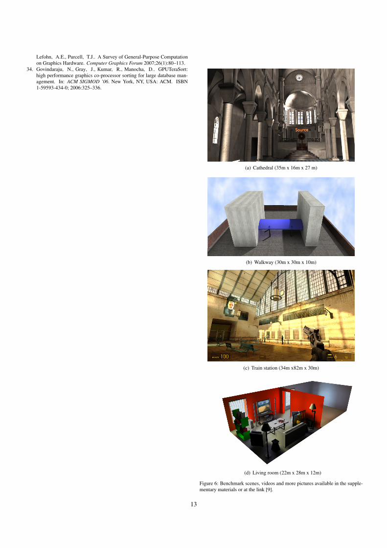
(a) Cathedral (35m x 16m x 27 m)

(b) Walkway (30m x 30m x 10m)

(c) Train station (34m x82m x 30m)

(d) Living room (22m x 28m x 12m)

Figure 6: Benchmark scenes, videos and more pictures available in the supple-mentary materials or at the link [9].

13