An Efficiency Measure for Dynamic Networks Modeled as Evolutionary Variational Inequalities

with Application to the Internet

and

Vulnerability Analysis

Anna Nagurney and Qiang Qiang

Department of Finance and Operations Management

Isenberg School of Management

University of Massachusetts

Amherst, Massachusetts 01003

January 2007; revised August 2007; January 2008

Netnomics 9 (2008), pp. 1-20.

Abstract: In this paper, we propose an efficiency/performance measure for dynamic net-

works, which have been modeled as evolutionary variational inequalities. Such applications

include the Internet. The measure, which captures demands, flows, and costs/latencies over

time, allows for the identification of the importance of the nodes and links and their rankings.

We provide both continuous time and discrete time versions of the efficiency measure. We

illustrate the efficiency measure for the time-dependent (demand-varying) Braess paradox

and demonstrate how it can be used to assess the most vulnerable nodes and links in terms

of the greatest impact of their removal on the efficiency/performance of the dynamic network

over time.

Keywords: network efficiency, performance measurement, dynamic networks, Internet,

Braess paradox, vulnerability analysis, critical network components, evolutionary variational

inequalities

1

1. Introduction

Networks provide the foundations for communication, transportation and logistics, en-

ergy provision, social interactions, as well as financing. The study of networks spans many

disciplines due to their wide application and importance. Indeed, today, the subject has

garnered renewed interest, since a spectrum of catastrophic events such as 9/11, the North

American electric power blackout of 2003, as well as Hurricane Katrina in 2005, among oth-

ers, have reinforced our need for and dependence on network systems (see, e.g., Nagurney

(2006)).

The Internet, in particular, as a telecommunications network, and with linkages to other

network systems, including transportation and financial ones, as well as energy systems, is

fundamental to the functioning of our modern societies and economies. Hence, an appropriate

efficiency measure and a means of identifying its critical nodes and links is essential to not

only the management of such a dynamic network but also to its very security. Clearly,

those nodes and links that are deemed most important are those that also merit greatest

protection.

In this paper, we propose a network efficiency measure for dynamic networks, which

have been modeled as evolutionary variational inequalities. Such dynamic networks include

the Internet (cf. Nagurney, Parkes, and Daniele (2007)). To-date, the network efficiency

measure proposed by Latora and Marchiori (2001), which is the sum of the inverses of the

shortest paths based on geodesic distances between nodes, multiplied by one over the number

of nodal pairs, has been applied to several network systems, including the MBTA subway

system in Boston and the Internet (cf. Latora and Marchiori (2003, 2004)). However, their

measure does not include behavior that would be associated with rerouting in the case

of nodal or link failures nor does it explicitly include traffic flows. Furthermore, it does

not capture the time dimension. Bienenstock and Bonacich (2003), in turn, focused on

social networks and their efficiency versus vulnerability and proposed a network efficiency

measure, which actually coincides with that of Latora and Marchiori (2001). More recently,

Jenelius, Petersen, and Mattsson (2006) proposed a network efficiency measure for congested

transportation networks but the measure requires that the network remain connected after

disruptions. Furthermore, it does not measure the usage of the network as demand varies

2

over time.

We use as the basis for our dynamic network measurement framework the time-dependent,

evolutionary variational inequality (EVI) model of the Internet proposed by Nagurney,

Parkes, and Daniele (2007). Indeed, since the demand for Internet resources itself is dynamic,

an underpinning modeling framework must be able to handle time-dependent constraints.

Roughgarden (2005) on page 10 notes that, “A network like the Internet is volatile. Its

traffic patterns can change quickly and dramatically ... The assumption of a static model is

therefore particularly suspect in such networks.”

It has been shown (cf. Roughgarden (2005) and the references therein) that distributed

routing, which is common in computer networks and, in particular, the Internet, and “selfish”

(or “source” routing in computer networks) routing, as occurs in the case of user-optimized

transportation networks, in which travelers select the minimum cost route between an origin

and destination, are one and the same if the cost functions associated with the links that

make up the paths/routes coincide with the lengths used to define the shortest paths. In this

paper, we assume that the costs on the links are congestion-dependent, that is, they depend

on the volume of the flow on the link. Note that network efficiency measurements based on

shortest path geodesic distances ignore this property of congested networks. We permit the

cost on a link to represent travel delay but we utilize “cost” functions since these are more

general conceptually than delay (or latency) functions and they can include, for example,

tolls associated with pricing, etc.

In addition, we emphasize that, in the case of transportation networks, it is travelers

that make the decisions as to the route selection between origin/destination (O/D) pairs

of nodes, whereas in the case of the Internet, it is algorithms, implemented in software,

that determine the shortest paths. Furthermore, we mention that analogues exist between

transportation networks and telecommunication networks and, in particular, the Internet, in

terms of decentralized decision-making, flows and costs, and even the Braess paradox, which

allow us to take advantage of such a connection (cf. Beckmann, McGuire, and Winsten

(1956), Beckmann (1967), Braess (1968), Dafermos and Sparrow (1969), Cantor and Gerla

(1974), Gallager (1977), Bertsekas and Tsitsiklis (1989), Bertsekas and Gallager (1992), Ran

and Boyce (1996), Korilis, Lazar, and Orda (1999), Boyce, Mahmassani, and Nagurney

3

(2005), Resende and Pardalos (2006), Nagurney, Parkes, and Daniele (2007)).

The evolutionary variational inequality methodology that Nagurney, Parkes, and Daniele

(2007) utilized for the formulation and analysis of the Internet is quite natural for several

reasons. First, historically, finite-dimensional variational inequality theory (cf. Smith (1979),

Dafermos (1980), Nagurney (1993), Patriksson (1994), and the references therein) has been

used to generalize static transportation network equilibrium models dating to the classic

work of Beckmann, McGuire, and Winsten (1956), which also forms the foundation for

selfish routing and decentralized decision-making on the Internet (see, e.g., Roughgarden

(2005)). Secondly, there has been much research activity devoted to the development of

models for dynamic transportation problems and it makes sense to exploit the connections

between transportation networks and the Internet (see also Nagurney and Dong (2002)

and Boyce, Mahmassani, and Nagurney (2005)). In addition, EVIs, which are infinite-

dimensional, have been used to model a variety of time-dependent applications, including

time-dependent spatial price problems, financial network problems, dynamic supply chains,

and electric power networks (cf. Daniele, Maugeri, and Oettli (1999), Daniele (2003, 2004),

Daniele (2006), Nagurney et al. (2007), and Nagurney (2006)). Hence, we believe that

they are a rather natural formalism for dynamic networks and the measurement of their

efficiency/performance.

The structure of the paper is as follows. In Section 2 we briefly recall the evolution-

ary variational inequality formulation of the Internet due to Nagurney, Parkes, and Daniele

(2007). In Section 3, we propose the efficiency measure for dynamic networks in both con-

tinuous time and discrete time forms. In Section 4, we apply the measure to the Braess

paradox network with time-varying demands to determine the network efficiency as well as

the importance rankings of the nodes and links. In Section 5, we summarize the results in

this paper and present our conclusions.

4

2. Evolutionary Variational Inequalities and the Internet

For definiteness, in this section, we review the evolutionary variational inequality model of

the Internet, recently proposed by Nagurney, Parkes, and Daniele (2007), but, for simplicity,

we consider the single class, rather than the multiclass version.

In particular, the Internet, a dynamic network par excellence, is modeled as a network

G = [N, L], consisting of the set of nodes N and the set of directed links L. The set of links

L consists of nL elements. The set of O/D pairs of nodes is denoted by W and consists of

nW elements. We denote the set of routes (with a route consisting of links) joining the O/D

pair w by Pw. We assume that the routes are acyclic. Let P with nP elements denote the

set of all routes connecting all the O/D pairs in the Internet. Links are denoted by a, b, etc;

routes by r, q, etc., and O/D pairs by w1, w2, etc. We assume that the Internet is traversed

by a single class of “job” or “task.”

Let dw(t) denote the demand, that is, the traffic generated, between O/D pair w at time

t. The flow on route r at time t, which is assumed to be nonnegative, is denoted by xr(t)

and the flow on link a at time t by fa(t).

Since the demands over time are assumed known, the following conservation of flow

equations must be satisfied at each t:

dw(t) =∑

r∈Pw

xr(t), ∀w ∈ W, (1)

that is, the demand associated with an O/D pair must be equal to the sum of the flows on

the routes that connect that O/D pair. Also, we must have that

0 ≤ xr(t) ≤ µr(t), ∀r ∈ P, (2)

where µr(t) denotes the capacity on route r at time t.

We group the demands at time t for all the O/D pairs into the nW -dimensional vec-

tor d(t) and the route flows at time t into the nP -dimensional vector x(t). The upper

bounds/capacities on the routes at time t are grouped into the nP -dimensional vector µ(t).

The link flows are related to the route flows, in turn, through the following conservation

5

of flow equations:

fa(t) =∑r∈P

xr(t)δar, ∀a ∈ L, (3)

where δar = 1 if link a is contained in route r, and δar = 0, otherwise. Hence, the flow on a

link is equal to the sum of the flows on routes that contain that link. All the link flows at

time t are grouped into the vector f(t), which is of dimension nL.

The cost on route r at time t is denoted by Cr(t) and the cost on a link a at time t by

ca(t). We allow the cost on a link, in general, to depend upon the entire vector of link flows

at time t, so that

ca(t) = ca(f(t)), ∀a ∈ L. (4)

In view of (3), we may write the link costs as a function of route flows, that is,

ca(x(t)) ≡ ca(f(t)), ∀a ∈ L. (5)

The costs on routes are related to costs on links through the following equations:

Cr(x(t)) =∑a∈L

ca(x(t))δar, ∀r ∈ P, (6)

which means that the cost on a route at a time t is equal to the sum of costs on links that

make up the route at time t. We group the route costs at time t into the vector C(t), which

is of dimension nP .

We now define the feasible set K. We consider the Hilbert space L = L2([0, T ] , RnP )

(where T denotes the time interval under consideration) given by

K =

x ∈ L2([0, T ] , RnP ) : 0 ≤ x(t) ≤ µ(t) a.e. in [0, T ];∑

p∈Pw

xp(t) = dw(t),∀w, a.e. in [0, T ]

.

(7)

We assume that the capacities µr(t), for all r, are in L and that the demands, dw ≥ 0,

for all w, are also in L. Further, we assume that

0 ≤ d(t) ≤ Φµ(t), a.e. on [0, T ], (8)

6

where Φ is the nW × nP -dimensional O/D pair-route incidence matrix, with element (w, r)

equal to 1 if route r is contained in Pw, and 0, otherwise. Due to (8), the feasible set Kis nonempty. As noted in Nagurney, Parkes, and Daniele (2007), K is also convex, closed,

and bounded. Note that we are not restricted as to the form that the time-varying demands

for the O/D pairs take since convexity is guaranteed even if the demands have a step-wise

structure, or are piecewise continuous.

The dual space of L is denoted by L∗. On L × L∗ we define the canonical bilinear form

by

〈〈G, x〉〉 :=∫ T

0〈G(t), x(t)〉dt, G ∈ L∗, x ∈ L. (9)

Furthermore, the cost mapping C : K → L∗, assigns to each flow trajectory x(·) ∈ K the

cost trajectory C(x(·)) ∈ L∗.

We now state the dynamic network equilibrium conditions governing the Internet, assum-

ing shortest path routing. These conditions are a generalization of the Wardropian (1952)

first principle of traffic behavior (see also, e.g., Beckmann, McGuire, and Winsten (1956),

Dafermos and Sparrow (1969), Dafermos (1980), and Nagurney (1993)) to include the time

dimension and capacities on the route flows. Of course, if the capacities are very large and

exceed the demand at each t, then the upper bounds are never attained by the route flows

and the conditions below will collapse, in the case of fixed time t, to the well-known static

network equilibrium conditions (see Dafermos and Sparrow (1969), Dafermos (1980), and

the references therein). The below is a special case of the multiclass network equilibrium

conditions stated in Nagurney, Parkes, and Daniele (2007); see also Daniele (2006).

Definition 1: Dynamic Network Equilibrium

A route flow pattern x∗ ∈ K is said to be a dynamic network equilibrium (according to the

generalization of Wardrop’s first principle), if, at each time t, only the minimum cost routes

not at their capacities are used (that is, have positive flow) for each O/D pair unless the flow

on a route is at its upper bound (in which case those routes’ costs can be lower than those on

the routes not at their capacities). The state can be expressed by the following equilibrium

conditions which must hold for every O/D pair w ∈ W , every route r ∈ Pw, and a.e. on

7

[0, T ]:

Cr(x∗(t))− λ∗w(t)

≤ 0, if x∗r(t) = µr(t),= 0, if 0 < x∗r(t) < µr(t),≥ 0, if x∗r(t) = 0.

(10)

Hence, conditions (10) state that all utilized routes not at their capacities connecting an

O/D pair have equal and minimal costs at each time t in [0, T ]. If a route flow is at its

capacity then its cost can be lower than the minimal cost for that O/D pair. Of course, if we

have that µr = ∞, for all routes r ∈ P , then the dynamic equilibrium conditions state that

all used routes connecting an O/D pair of nodes have equal and minimal route costs at each

time t. For fixed t, the latter conditions coincide with a single class version of Wardrop’s

first principle (see Dafermos and Sparrow (1969) governing static transportation network

equilibrium problems). Note that this concept has also been applied to static models of the

Internet (cf. Roughgarden (2005) and the references therein).

In the above discussion, we assume that the general “cost” on links and paths is “in-

stantaneous,” which solely depends on the current network flows and demands. Such an

assumption is relatively general and can be easily extended to the discrete-time case, which

will be discussed in the following section. Indeed, in the discrete-time case, demand is as-

sumed to be constant during each time interval and, therefore, the link and path costs can

be interpreted as the average costs based on the flows in that particular time interval. Fur-

thermore, similar data and computer communication network models and analysis, but in

the discrete-time case, have also been studied by Bertsekas and Gallager (1992).

The standard form of the EVI that we work with is:

determine x∗ ∈ K such that 〈〈F (x∗), x− x∗〉〉 ≥ 0, ∀x ∈ K. (11)

We now state the following theorem, which is an adaptation of Theorem 1 in Nagurney,

Parkes, and Daniele (2007) to the single-class case; see that reference for a proof.

8

Theorem 1

x∗ ∈ K is an equilibrium flow according to Definition 1 if and only if it satisfies the evolu-

tionary variational inequality:∫ T

0〈C(x∗(t)), x(t)− x∗(t)〉dt ≥ 0, ∀x ∈ K. (12)

Furthermore, for completeness, we also provide some existence results:

Theorem 2 (cf. Daniele, Maugeri, and Oettli (1999) and Daniele (2006))

If C in (12) satisfies any of the following conditions:

1. C is hemicontinuous with respect to the strong topology on K, and there exist A ⊆ Knonempty, compact, and B ⊆ K compact such that, for every y ∈ K \ A, there exists

x ∈ B with 〈〈C(x), y − x〉〉 < 0;

2. C is hemicontinuous with respect to the weak topology on K;

3. C is pseudomonotone and hemicontinuous along line segments,

then the EVI problem (12) admits a solution over the constraint set K.

Recall that C :→ L∗, where K is convex, is said to be

pseudomonotone if and only if, for all x, y ∈ K

〈〈C(x), y − x〉〉 ≤ 0 ⇒ 〈〈C(y), x− y〉〉 ≤ 0;

hemicontinuous if and only if, for all y ∈ K, the function ξ 7→ 〈〈C(ξ), y − ξ〉〉 is upper

semicontinuous on K;

hemicontinuous along line segments if and only if, for all x, y ∈ K, the function ξ 7→〈〈C(ξ), y − x〉〉 is upper semicontinuous on the line segment [x, y].

9

Moreover, if C is strictly monotone, then the solution of (12) is unique (see, e.g., Kinder-

lehrer and Stampacchia (1980)).

Daniele, Maugeri, and Oettli (1999) presented dynamic network equilibrium conditions

for transportation networks. Here, we state the dynamic equilibrium conditions in a manner

that is more transparent (cf. (10)), noting that the lower bounds on the route flows on the

Internet will be zero.

We note that the solution of finite-dimensional variational inequalities is at quite an ad-

vanced state (cf. Nagurney (1993)). The solution of evolutionary variational inequalities,

which are infinite-dimensional, is a topic discussed in the books by Daniele (2006) and Nagur-

ney (2006) as well as in the papers by Cojocaru, Daniele, and Nagurney (2005, 2006) and

in Barbagallo (2007). In particular, under certain conditions, an evolutionary variational

inequality of the form (12) can be solved at discrete points in time and the solutions then

interpolated. Hence, the advances in the computation of finite-dimensional variational in-

equalities, with many network equilibrium problems solved to-date, may be exploited for the

effective solution of the EVI for dynamic networks.

We now present a small dynamic network numerical example.

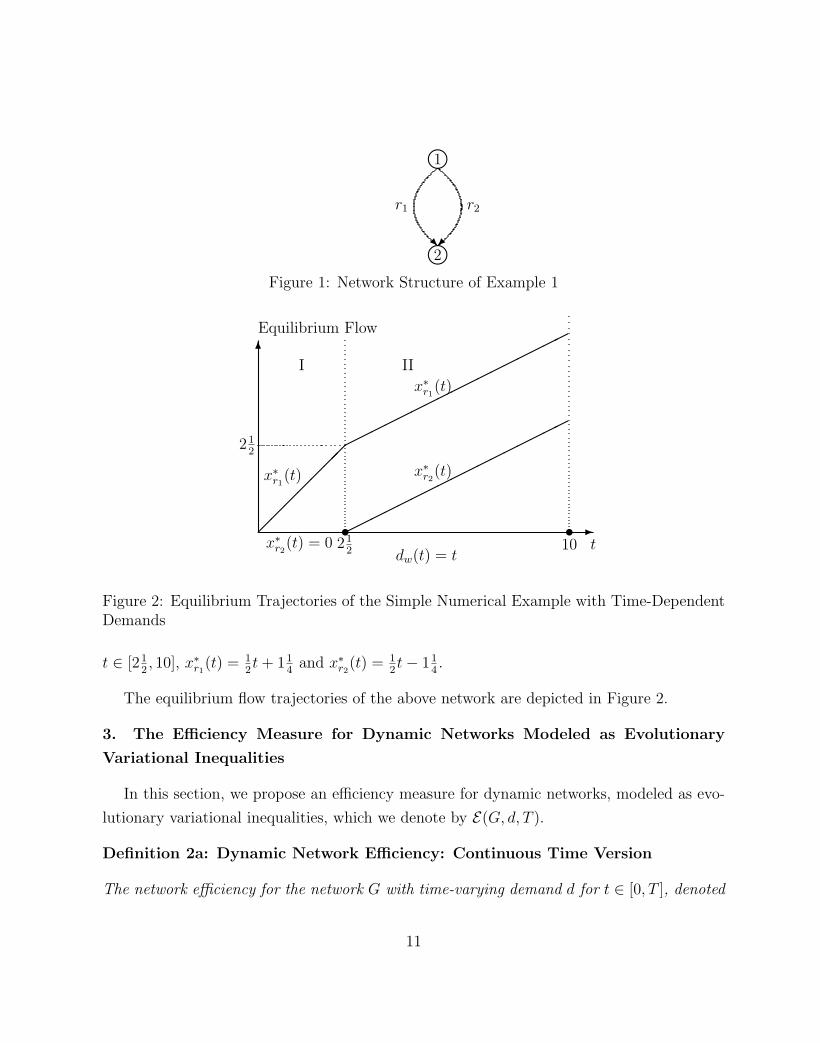
Example 1: A Simple Numerical Example

Consider a network (small subnetwork of the Internet) consisting of two nodes and two links

as in Figure 1. Since the routes consist of single links we work with the routes directly as in

Figure 1. The route costs are:

Cr1(x(t)) = 2xr1(t) + 5, Cr2(x(t)) = 2xr2(t) + 10.

Also, we assume that the route capacities are: µr1(t) = µr2(t) = ∞.

The time horizon is [0, 10]. There is a single O/D pair w = (1, 2) and the time-varying

demand is assumed to be dw(t) = t.

Given the special structure of the network in Figure 1 and the linearity and separability of

the route cost functions, it is easy to determine the equilibrium route trajectories satisfying

(10), or, equivalently, (12), and they are: for t ∈ [0, 212], x∗r1

(t) = t and x∗r2(t) = 0, and for

10

m

m

2

1

r1 r2

R

Figure 1: Network Structure of Example 1

-

6

��

��

���

x∗r2(t) = 0

x∗r1(t)

I II

tt

���������

������

��

������

�����������

x∗r1(t)

x∗r2(t)

dw(t) = t1021

2

212

Equilibrium Flow

t

Figure 2: Equilibrium Trajectories of the Simple Numerical Example with Time-DependentDemands

t ∈ [212, 10], x∗r1

(t) = 12t + 11

4and x∗r2

(t) = 12t− 11

4.

The equilibrium flow trajectories of the above network are depicted in Figure 2.

3. The Efficiency Measure for Dynamic Networks Modeled as Evolutionary

Variational Inequalities

In this section, we propose an efficiency measure for dynamic networks, modeled as evo-

lutionary variational inequalities, which we denote by E(G, d, T ).

Definition 2a: Dynamic Network Efficiency: Continuous Time Version

The network efficiency for the network G with time-varying demand d for t ∈ [0, T ], denoted

11

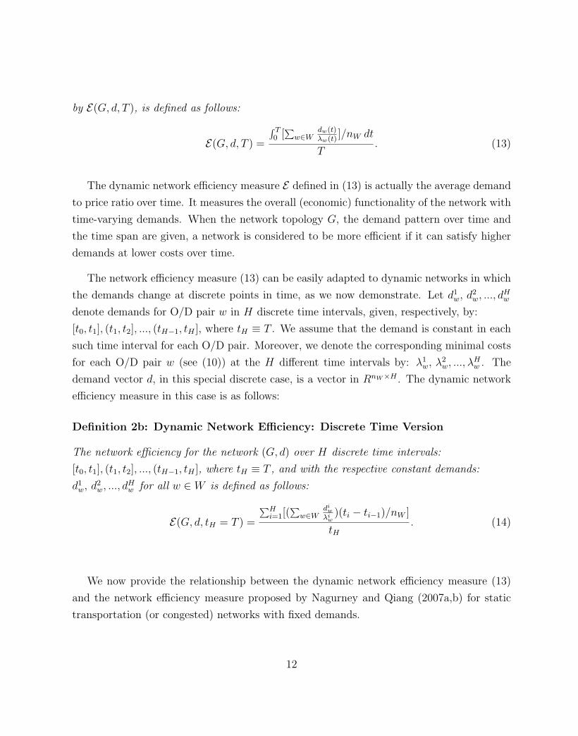
by E(G, d, T ), is defined as follows:

E(G, d, T ) =

∫ T0 [

∑w∈W

dw(t)λw(t)

]/nW dt

T. (13)

The dynamic network efficiency measure E defined in (13) is actually the average demand

to price ratio over time. It measures the overall (economic) functionality of the network with

time-varying demands. When the network topology G, the demand pattern over time and

the time span are given, a network is considered to be more efficient if it can satisfy higher

demands at lower costs over time.

The network efficiency measure (13) can be easily adapted to dynamic networks in which

the demands change at discrete points in time, as we now demonstrate. Let d1w, d2

w, ..., dHw

denote demands for O/D pair w in H discrete time intervals, given, respectively, by:

[t0, t1], (t1, t2], ..., (tH−1, tH ], where tH ≡ T . We assume that the demand is constant in each

such time interval for each O/D pair. Moreover, we denote the corresponding minimal costs

for each O/D pair w (see (10)) at the H different time intervals by: λ1w, λ2

w, ..., λHw . The

demand vector d, in this special discrete case, is a vector in RnW×H . The dynamic network

efficiency measure in this case is as follows:

Definition 2b: Dynamic Network Efficiency: Discrete Time Version

The network efficiency for the network (G, d) over H discrete time intervals:

[t0, t1], (t1, t2], ..., (tH−1, tH ], where tH ≡ T , and with the respective constant demands:

d1w, d2

w, ..., dHw for all w ∈ W is defined as follows:

E(G, d, tH = T ) =

∑Hi=1[(

∑w∈W

diw

λiw)(ti − ti−1)/nW ]

tH. (14)

We now provide the relationship between the dynamic network efficiency measure (13)

and the network efficiency measure proposed by Nagurney and Qiang (2007a,b) for static

transportation (or congested) networks with fixed demands.

12

Theorem 3

Assume that dw(t) = dw, for all O/D pairs w ∈ W and for t ∈ [0, T ]. Then, the dynamic

network efficiency measure (13) collapses to the Nagurney and Qiang (2007a, b) measure:

E =1

nW

∑w∈W

dw

λw

. (15)

Proof: Since the dw’s are fixed over the time horizon [0, T ], the minimal equilibrium route

costs for each O/D pair, denoted by λw, ∀w ∈ W , are also fixed over the time horizon.

Substituting these terms into (13), we obtain:

E(G, d, T ) =

∫ T0 [

∑w∈W

dw

λw]/nW dt

T=

T

T[∑

w∈W

dw

λw

]/nW = [∑

w∈W

dw

λw

]/nW . (16)

But the right-most expression in (16) is precisely the Nagurney and Qiang (2007a, b) measure

for static traffic network equilibrium problems. 2

Several points merit some discussion here. First, one of the advantages of the above

measure is that it allows us to study the network efficiency where there exist disconnected

O/D pairs. Such a feature is extremely useful in assessing the network functionality under

partial disruptions whereas traditional measures, such as the total network cost over time, are

no longer applicable (cf. Roughgarden (2005)). An illustrative example will be given later in

this section. Second, in the above definition, we consider the network model without explicit

edge, that is, link, capacity constraints. It is well-known in the transportation literature

that edge capacities can be implicitly included in the link travel cost functions in which

case the travel time tends to infinity as the link flows approach their respective capacities

(cf. Daganzo (1977a, b)). A network model with explicit edge capacity constraints was

studied by Patriksson (1994), who generalized link costs to reformulate the network as an

equivalent uncapacitated network. Hence, in such a model, λw(t) in (13) can be interpreted

as a generalized cost. Nevertheless, a discussion of the distinction and the relationships

between the two approaches is not the focus of the current paper. We will devote our future

research to the network model with explicit edge capacity constraints.

13

The importance of a network component in the dynamic network case is the same as

that defined in Nagurney and Qiang (2007a, b), but with the static efficiency measure now

replaced by the dynamic network efficiency measure given by (13) in the continuous case

and by (14) in the discrete case. Hence, we have the following:

Definition 3: Importance of a Network Component

The importance of network component g of network G with demand d over time horizon T

is defined as follows:

I(g, d, T ) =E(G, d, T )− E(G− g, d, T )

E(G, d, T )(17)

where E(G− g, d, T ) is the dynamic network efficiency after component g is removed.

In studying the importance of a network component, the elimination of a link is treated

in the above measure by removing that link while the removal of a node is managed by

removing the links entering and exiting that node. In the case that the removal results in

no path/route connecting an O/D pair, we simply assign the demand for that O/D pair to

an abstract path with a cost of infinity. Hence, our measure is well-defined even in the case

of disconnected networks; see also Nagurney and Qiang (2007a, b). Additional theoretical

properties of the static measure can be found in Qiang and Nagurney (2008).

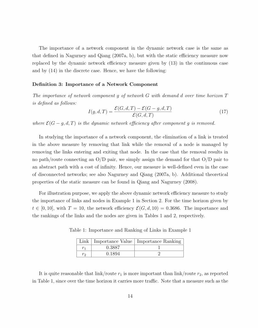
For illustration purpose, we apply the above dynamic network efficiency measure to study

the importance of links and nodes in Example 1 in Section 2. For the time horizon given by

t ∈ [0, 10], with T = 10, the network efficiency E(G, d, 10) = 0.3686. The importance and

the rankings of the links and the nodes are given in Tables 1 and 2, respectively.

Table 1: Importance and Ranking of Links in Example 1

Link Importance Value Importance Rankingr1 0.3887 1r2 0.1894 2

It is quite reasonable that link/route r1 is more important than link/route r2, as reported

in Table 1, since over the time horizon it carries more traffic. Note that a measure such as the

14

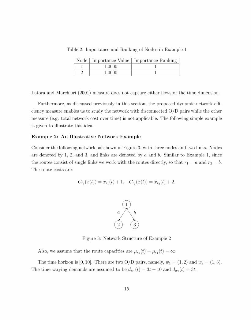
Table 2: Importance and Ranking of Nodes in Example 1

Node Importance Value Importance Ranking1 1.0000 12 1.0000 1

Latora and Marchiori (2001) measure does not capture either flows or the time dimension.

Furthermore, as discussed previously in this section, the proposed dynamic network effi-

ciency measure enables us to study the network with disconnected O/D pairs while the other

measure (e.g. total network cost over time) is not applicable. The following simple example

is given to illustrate this idea.

Example 2: An Illustrative Network Example

Consider the following network, as shown in Figure 3, with three nodes and two links. Nodes

are denoted by 1, 2, and 3, and links are denoted by a and b. Similar to Example 1, since

the routes consist of single links we work with the routes directly, so that r1 = a and r2 = b.

The route costs are:

Cr1(x(t)) = xr1(t) + 1, Cr2(x(t)) = xr2(t) + 2.

��������2 3

�

JJJ

����1

a b

Figure 3: Network Structure of Example 2

Also, we assume that the route capacities are µr1(t) = µr1(t) = ∞.

The time horizon is [0, 10]. There are two O/D pairs, namely, w1 = (1, 2) and w2 = (1, 3).

The time-varying demands are assumed to be dw1(t) = 3t + 10 and dw2(t) = 3t.

15

Given the special structure of the network, it is easy to determine the equilibrium route

trajectories satisfying (10), or equivalently, (12), and they are: x∗r1(t) = 3t + 10 and x∗r2

(t) =

3t.

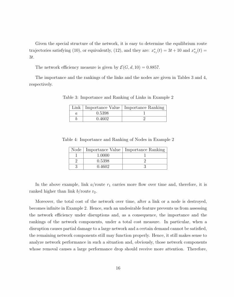
The network efficiency measure is given by E(G, d, 10) = 0.8857.

The importance and the rankings of the links and the nodes are given in Tables 3 and 4,

respectively.

Table 3: Importance and Ranking of Links in Example 2

Link Importance Value Importance Rankinga 0.5398 1b 0.4602 2

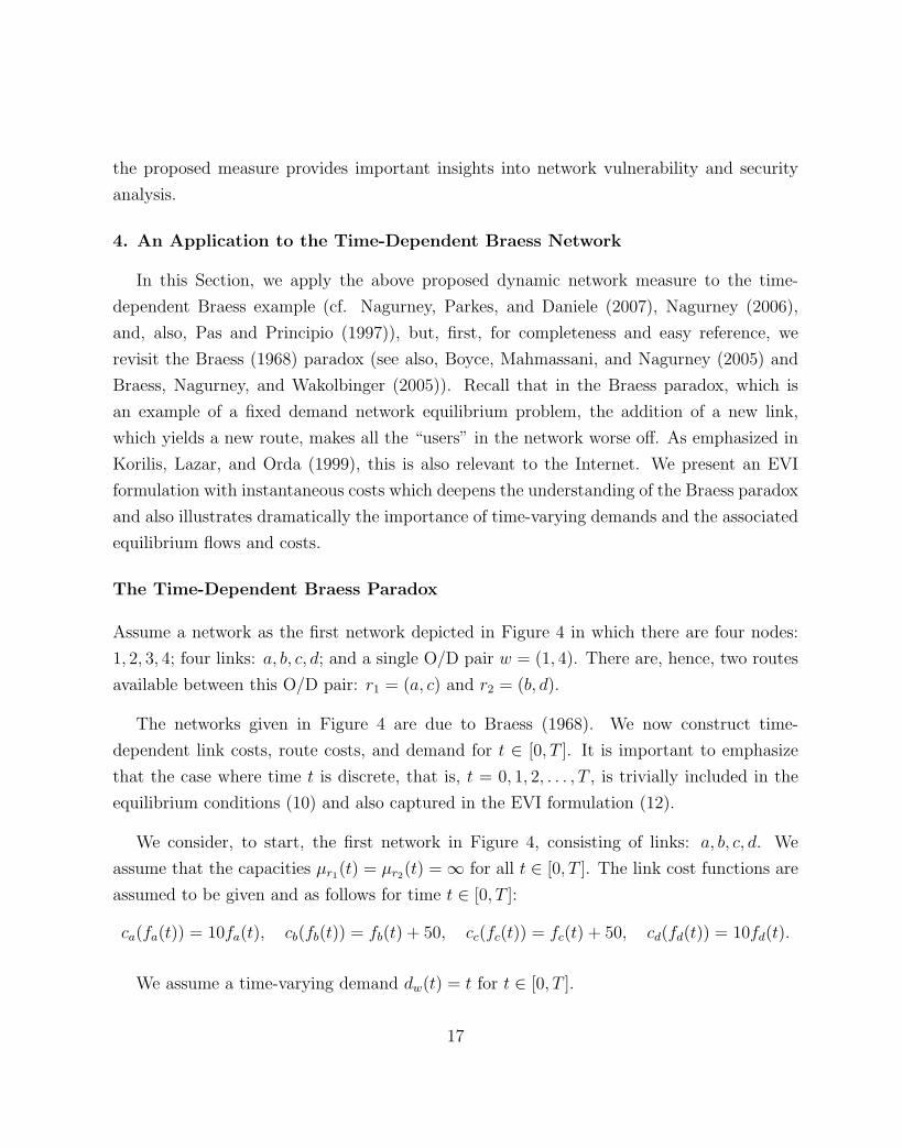
Table 4: Importance and Ranking of Nodes in Example 2

Node Importance Value Importance Ranking1 1.0000 12 0.5398 23 0.4602 3

In the above example, link a/route r1 carries more flow over time and, therefore, it is

ranked higher than link b/route r2.

Moreover, the total cost of the network over time, after a link or a node is destroyed,

becomes infinite in Example 2. Hence, such an undesirable feature prevents us from assessing

the network efficiency under disruptions and, as a consequence, the importance and the

rankings of the network components, under a total cost measure. In particular, when a

disruption causes partial damage to a large network and a certain demand cannot be satisfied,

the remaining network components still may function properly. Hence, it still makes sense to

analyze network performance in such a situation and, obviously, those network components

whose removal causes a large performance drop should receive more attention. Therefore,

16

the proposed measure provides important insights into network vulnerability and security

analysis.

4. An Application to the Time-Dependent Braess Network

In this Section, we apply the above proposed dynamic network measure to the time-

dependent Braess example (cf. Nagurney, Parkes, and Daniele (2007), Nagurney (2006),

and, also, Pas and Principio (1997)), but, first, for completeness and easy reference, we

revisit the Braess (1968) paradox (see also, Boyce, Mahmassani, and Nagurney (2005) and

Braess, Nagurney, and Wakolbinger (2005)). Recall that in the Braess paradox, which is

an example of a fixed demand network equilibrium problem, the addition of a new link,

which yields a new route, makes all the “users” in the network worse off. As emphasized in

Korilis, Lazar, and Orda (1999), this is also relevant to the Internet. We present an EVI

formulation with instantaneous costs which deepens the understanding of the Braess paradox

and also illustrates dramatically the importance of time-varying demands and the associated

equilibrium flows and costs.

The Time-Dependent Braess Paradox

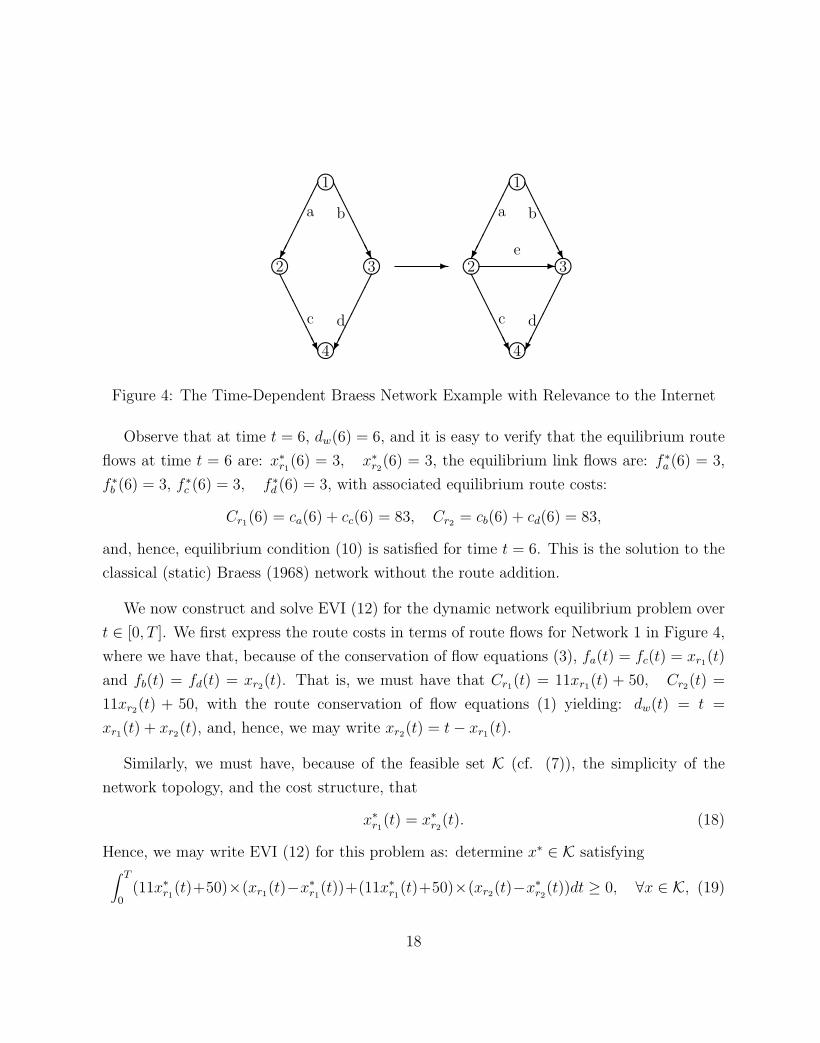
Assume a network as the first network depicted in Figure 4 in which there are four nodes:

1, 2, 3, 4; four links: a, b, c, d; and a single O/D pair w = (1, 4). There are, hence, two routes

available between this O/D pair: r1 = (a, c) and r2 = (b, d).

The networks given in Figure 4 are due to Braess (1968). We now construct time-

dependent link costs, route costs, and demand for t ∈ [0, T ]. It is important to emphasize

that the case where time t is discrete, that is, t = 0, 1, 2, . . . , T , is trivially included in the

equilibrium conditions (10) and also captured in the EVI formulation (12).

We consider, to start, the first network in Figure 4, consisting of links: a, b, c, d. We

assume that the capacities µr1(t) = µr2(t) = ∞ for all t ∈ [0, T ]. The link cost functions are

assumed to be given and as follows for time t ∈ [0, T ]:

ca(fa(t)) = 10fa(t), cb(fb(t)) = fb(t) + 50, cc(fc(t)) = fc(t) + 50, cd(fd(t)) = 10fd(t).

We assume a time-varying demand dw(t) = t for t ∈ [0, T ].

17

k

k

k k

1

4

2 3AAAAAAU

��

��

���

��

��

���

AAAAAAU

c

a

d

b

k

k

k k

1

4

2 3AAAAAAU

��

��

���

��

��

���

AAAAAAU

-

c

a

d

b

e-

Figure 4: The Time-Dependent Braess Network Example with Relevance to the Internet

Observe that at time t = 6, dw(6) = 6, and it is easy to verify that the equilibrium route

flows at time t = 6 are: x∗r1(6) = 3, x∗r2

(6) = 3, the equilibrium link flows are: f ∗a (6) = 3,

f ∗b (6) = 3, f ∗c (6) = 3, f ∗d (6) = 3, with associated equilibrium route costs:

Cr1(6) = ca(6) + cc(6) = 83, Cr2 = cb(6) + cd(6) = 83,

and, hence, equilibrium condition (10) is satisfied for time t = 6. This is the solution to the

classical (static) Braess (1968) network without the route addition.

We now construct and solve EVI (12) for the dynamic network equilibrium problem over

t ∈ [0, T ]. We first express the route costs in terms of route flows for Network 1 in Figure 4,

where we have that, because of the conservation of flow equations (3), fa(t) = fc(t) = xr1(t)

and fb(t) = fd(t) = xr2(t). That is, we must have that Cr1(t) = 11xr1(t) + 50, Cr2(t) =

11xr2(t) + 50, with the route conservation of flow equations (1) yielding: dw(t) = t =

xr1(t) + xr2(t), and, hence, we may write xr2(t) = t− xr1(t).

Similarly, we must have, because of the feasible set K (cf. (7)), the simplicity of the

network topology, and the cost structure, that

x∗r1(t) = x∗r2

(t). (18)

Hence, we may write EVI (12) for this problem as: determine x∗ ∈ K satisfying∫ T

0(11x∗r1

(t)+50)×(xr1(t)−x∗r1(t))+(11x∗r1

(t)+50)×(xr2(t)−x∗r2(t))dt ≥ 0, ∀x ∈ K, (19)

18

which, in view of the feasibility condition: xr1(t) + xr2(t) = t, implies that (19) can be

expressed as:∫ T

0(11x∗r1

(t)+50)× (xr1(t)−x∗r1(t))+ (11x∗r1

(t)+50)× (t−xr1(t)−x∗r1(t))dt ≥ 0, ∀x ∈ K,

(20)

which, after algebraic simplification, is∫ T

0(11x∗r1

(t) + 50)× (t− 2x∗r1(t))dt ≥ 0, ∀x ∈ K. (21)

But, (21) implies that: 2x∗r1(t) = t; for t ∈ [0, T ] or x∗r1

(t) = t2. Hence, we also have that

x∗r2(t) = t

2.

Moreover, the equilibrium route costs for t ∈ [0, T ] are given by: Cr1(x∗r1

(t)) = 512t+50 =

Cr2(x∗r2

(t)) = 512t + 50, and, clearly, equilibrium conditions (10) hold for ∈ [0, T ] a.e.

Assume now that, as depicted in Figure 4, a new link “e”, joining node 2 to node 3 is

added to the original network, with cost ce(fe(t)) = fe(t) + 10 for t ∈ [0, T ]. The addition of

this link creates a new route r3 = (a, e, d) that is available for the Internet traffic. Assume

that the time-varying demand is still given by dw(t) = t. Note, that for t = 6, for example,

the original equilibrium flow distribution pattern xr1(6) = 3 and xr2(6) = 3 is no longer an

equilibrium pattern, since at this level of flow the cost on route r3, Cr3(6) = 70. Hence, the

traffic from routes r1 and r2 would be switched to route r3.

The equilibrium flow pattern at time t = 6 on the new network (which would correspond to

the classic Braess paradox in a static network equilibrium setting) is: x∗r1(6) = 2, x∗r2

(6) = 2,

x∗r3(6) = 2, with equilibrium link flows: f ∗a (6) = 4, f ∗b (6) = 2, f ∗c (6) = 2, f ∗e (6) = 2,

f ∗d (6) = 4, and with associated equilibrium route costs:

Cr1(6) = 92, Cr2(6) = 92, Cr3(6) = 92.

Indeed, one can verify that any reallocation of the route flows would yield a higher cost on

a route.

Note that, with the route addition, the cost at time t = 6 increased for every “user” of the

network from 83 to 92 without a change in the demand or traffic rate! This is the classical

Braess paradox.

19

-

6

��

��

��

��

x∗r1(t) = x∗r2

(t) = 0

x∗r3(t)

I

QQ

QQ

QQ

QQ

QQ

QQt

II

Braess Paradox Occurs

,,

,,

,,

,,

,,

,, t88

9

x∗r1(t) = x∗r2

(t)

New Route is Not Used

dw(t) = t

x∗r3(t)

3 711

x∗r1(t) = x∗r2

(t)

x∗r3(t) = 0

��

��

��

��

��

��III

449

Equilibrium Flow

t

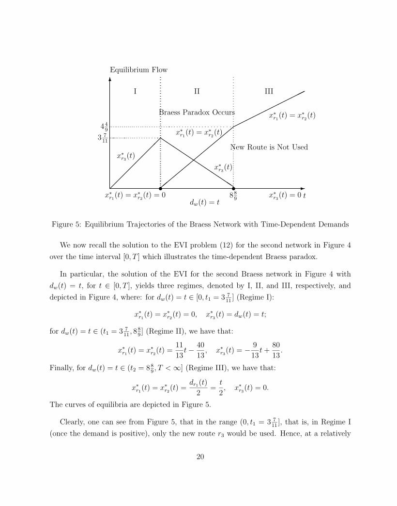
Figure 5: Equilibrium Trajectories of the Braess Network with Time-Dependent Demands

We now recall the solution to the EVI problem (12) for the second network in Figure 4

over the time interval [0, T ] which illustrates the time-dependent Braess paradox.

In particular, the solution of the EVI for the second Braess network in Figure 4 with

dw(t) = t, for t ∈ [0, T ], yields three regimes, denoted by I, II, and III, respectively, and

depicted in Figure 4, where: for dw(t) = t ∈ [0, t1 = 3 711

] (Regime I):

x∗r1(t) = x∗r2

(t) = 0, x∗r3(t) = dw(t) = t;

for dw(t) = t ∈ (t1 = 3 711

, 889] (Regime II), we have that:

x∗r1(t) = x∗r2

(t) =11

13t− 40

13, x∗r3

(t) = − 9

13t +

80

13.

Finally, for dw(t) = t ∈ (t2 = 889, T < ∞] (Regime III), we have that:

x∗r1(t) = x∗r2

(t) =dr1(t)

2=

t

2, x∗r3

(t) = 0.

The curves of equilibria are depicted in Figure 5.

Clearly, one can see from Figure 5, that in the range (0, t1 = 3 711

], that is, in Regime I

(once the demand is positive), only the new route r3 would be used. Hence, at a relatively

20

low level of demand, up to a value of 3 711

, only the new route is used. In the range of

demands: (3 711

, 889], that is, Regime II, all three routes are used, and in this range the Braess

paradox occurs. Finally, once the demand (recall that dw(t) = t here) exceeds 889

and we are

in Regime III, then the new route is never used! Thus, the use of an EVI formulation reveals

that over time the Braess paradox is even more profound and the addition of a new route

may result in the route never being used. Finally, if the demand lies within a particular

range, then the addition of a new route may result in everyone being worse off, since it

results in higher costs than before the route/link was added to the network.

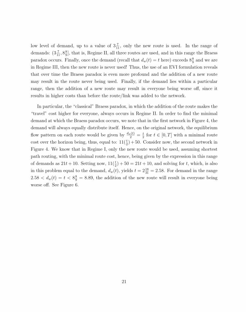
In particular, the “classical” Braess paradox, in which the addition of the route makes the

“travel” cost higher for everyone, always occurs in Regime II. In order to find the minimal

demand at which the Braess paradox occurs, we note that in the first network in Figure 4, the

demand will always equally distribute itself. Hence, on the original network, the equilibrium

flow pattern on each route would be given by dw(t)2

= t2

for t ∈ [0, T ] with a minimal route

cost over the horizon being, thus, equal to: 11( t2)+50. Consider now, the second network in

Figure 4. We know that in Regime I, only the new route would be used, assuming shortest

path routing, with the minimal route cost, hence, being given by the expression in this range

of demands as 21t + 10. Setting now, 11( t2) + 50 = 21t + 10, and solving for t, which, is also

in this problem equal to the demand, dw(t), yields t = 21831

= 2.58. For demand in the range

2.58 < dw(t) = t < 889

= 8.89, the addition of the new route will result in everyone being

worse off. See Figure 6.

21

-

6

��

��

��

��

��

��

��

��

��

��

��������������������

Minimum Used Route Cost

dw(t) = tt = 2.58

Network 2 (with route added)λ∗w(t) = 21t + 10

Network 1λ∗w(t) = 11(t/2) + 50

Figure 6: Minimum Used Route Costs for Braess Networks 1 and 2

For both networks in Figure 4, with the associated link and route cost functions, it is

easy to verify that the corresponding vector of route costs C(x) is strictly monotone (cf.

Nagurney (1993) and Daniele (2006)) in route flows x, that is,

〈〈C(x1)− C(x2), x1 − x2〉〉 > 0, ∀x1, x2 ∈ K, x1 6= x2,

since the Jacobian of the route costs is strictly diagonally dominant at each t and, thus,

positive definite. Hence, the corresponding equilibrium route flow solutions x∗(t) will be

unique.

Network Efficiency of the Dynamic Braess Network and Importance Rankings

of Nodes and Links Over the Time Horizon

Let us now consider the second dynamic Braess network in Figure 4 for t ∈ [0, 10]. As shown

in Nagurney, Parkes, and Daniele (2007) and recalled above, different routes (and links)

22

are used in different demand ranges. Therefore, it is interesting and relevant to study the

network efficiency and the importance of the network components over the time horizon.

Since in the above example, the demand varies continuously over time, the formula (13) is

used to compute the network efficiency. The computations for both (13) and for (17) were

done using Matlab (see www.mathworks.com).

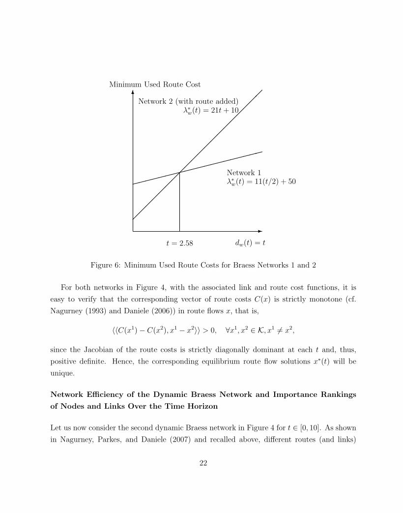
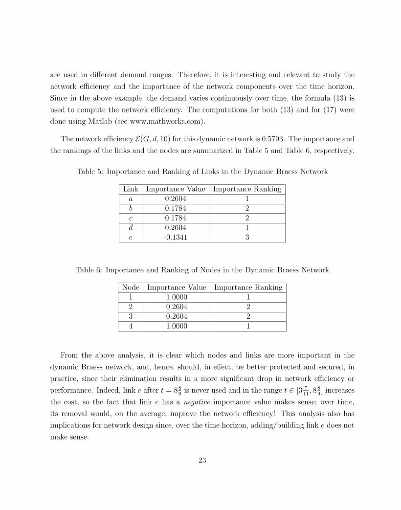
The network efficiency E(G, d, 10) for this dynamic network is 0.5793. The importance and

the rankings of the links and the nodes are summarized in Table 5 and Table 6, respectively.

Table 5: Importance and Ranking of Links in the Dynamic Braess Network

Link Importance Value Importance Rankinga 0.2604 1b 0.1784 2c 0.1784 2d 0.2604 1e -0.1341 3

Table 6: Importance and Ranking of Nodes in the Dynamic Braess Network

Node Importance Value Importance Ranking1 1.0000 12 0.2604 23 0.2604 24 1.0000 1

From the above analysis, it is clear which nodes and links are more important in the

dynamic Braess network, and, hence, should, in effect, be better protected and secured, in

practice, since their elimination results in a more significant drop in network efficiency or

performance. Indeed, link e after t = 889

is never used and in the range t ∈ [3 711

, 889] increases

the cost, so the fact that link e has a negative importance value makes sense; over time,

its removal would, on the average, improve the network efficiency! This analysis also has

implications for network design since, over the time horizon, adding/building link e does not

make sense.

23

5. Summary and Conclusions

In this paper, we proposed a network efficiency measure that can be used for dynamic

networks, formulated as evolutionary variational inequalities, including the Internet. The

network efficiency measure captures costs/latencies on networks with time-varying demands.

We provided both a continuous time version of the efficiency measure and a discrete version

and then showed that the dynamic network efficiency measure in the case of fixed demands

for all the origin/destination pairs over time collapses to the recently proposed measure in

Nagurney and Qiang (2007a, b) for transportation (as well as other congested) networks,

when such problems are formulated as network equilibrium problems in a static setting. The

novelty of the measure lies in that it enables us to assess the network performance without

worrying about the connectivity assumption and further, it can be utilized to study the

importance of network components under changing demands over the time horizon of interest.

To the best of our knowledge, this is the first, rigorous, and well-defined, dynamic network

efficiency measure. Such a tool, we expect, will be quite useful for security purposes since

the dynamic network itself will be most vulnerable, as measured by the drop in efficiency,

if the most important nodes (or links) are removed, due to, for example, structural failures,

natural disasters, terrorist attacks, etc.

We illustrated the formalism on three dynamic network examples, including the time-

dependent Braess paradox. From the results of the importance rankings of individual nodes

and links, we can see that when evaluating the vulnerability of a network, all the relevant

information regarding the demands, the flows, and the costs over time has to be taken into

consideration.

Future research will include the application of the results in this paper to large-scale

dynamic networks in telecommunication applications as well as other applications, such as

electric power supply chain networks (cf. Nagurney et al. (2007)). Also, we hope to use the

proposed network measure to study network robustness and reliability under uncertainty.

Finally, it would be very interesting to extend the results in this paper to generalize the

measure to the case of price-dependent, time-varying demands, the static version of which

was proposed by Qiang and Nagurney (2008).

24

Acknowledgments

The authors are grateful to the four anonymous reviewers for helpful comments and sugges-

tions on an earlier version of this paper.

This research was supported, in part, by NSF Grant No.: IIS-0002647, under the Manage-

ment of Knowledge Intensive Dynamic Systems (MKIDS) program. The first author also

acknowledges support from the John F. Smith Memorial Fund at the University of Mas-

sachusetts at Amherst. The support provided is very much appreciated.

References

Barbagallo, A. (2007), Regularity Results for Time-Dependent Variational Inequalities and

Quasi-Variational Inequalities and Application to the Calculation of Dynamic Traffic Net-

work, Mathematical Models and Methods in Applied Sciences 17, 277-304.

Beckmann, M. J.(1967) On the Theory of Traffic Flows in Networks, Traffic Quarterly 21,

109-116.

Beckmann, M. J., McGuire, C. B., and Winsten, C. B. (1956) Studies in the Economics of

Transportation, Yale University Press, New Haven, Connecticut.

Bertsekas, D. P., and Gallager, R. G. (1992) Data Networks 2nd Ed., Prentice-Hall, Engle-

wood Cliffs, New Jersey.

Bertsekas, D. P., and Tsitsiklis, J. N. (1997) Parallel and Distributed Computation: Numer-

ical Methods, Prentice-Hall, Englewood Cliffs, New Jersey.

Bienenstock, E. J., and Bonacich, P. (2003) Balancing Efficiency and Vulnerability in Social

Networks, in Dynamic Social Network Modeling and Analysis: Workshop Summary and

Papers , The National Academy of Sciences, pp. 253-264.

Boyce, D.E., Mahmassani, H. S., and Nagurney, A. (2005) A Retrospective of Beckmann,

McGuire, and Winsten’s Studies in the Economics of Transportation, Papers in Regional

Science 84, 85-103.

Braess, D. (1968) Uber ein Paradoxon aus der Verkehrsplanung, Unternehmensforschung 12,

25

258-268.

Braess, D., Nagurney, A., and Wakolbinger, T. (2005) On a Paradox of Traffic Planning,

Translation of the 1968 Article by Braess, Transportation Science 39, 446-450.

Cantor, D. G., and Gerla, M. (1974) Optimal Routing in a Packet-Switched Computer

Network, IEEE Transactions on Computers 23, 1062-1069.

Cojocaru, M.-G., Daniele, P., and Nagurney, A. (2005) Projected Dynamical Systems and

Evolutionary Variational Inequalities, Journal of Optimization Theory and Applications 27,

1-15.

Cojocaru, M.-G., Daniele, P., and Nagurney, A. (2006) Double-Layered Dynamics: A Unified

Theory of Projected Dynamical Systems and Evolutionary Variational Inequalities, European

Journal of Operational Research 175, 494-507.

Dafermos, S. (1980) Traffic Equilibrium and Variational Inequalities, Transportation Science

14, 42-54.

Daganzo, C. F. (1977a) On the Traffic Assignment Problem with Flow Dependent Costs-I,

Transportation Research 11, 433-437.

Daganzo, C. F. (1977b) On the Traffic Assignment Problem with Flow Dependent Costs-II,

Transportation Research 11, 439-441.

Dafermos, S. C., and Sparrow, F. T. (1969) The Traffic Assignment Problem for a General

Network, Journal of Research of the National Bureau of Standards 73B, 91-118.

Daniele, P. (2003) Evolutionary Variational Inequalities and Economic Models for Demand

Supply Markets, Mathematical Models and Methods in Applied Sciences 4, 471-489.

Daniele, P. (2004) Time-Dependent Spatial Price Equilibrium Problem: Existence and Sta-

bility Results for the Quantity Formulation Model, Journal of Global Optimization 28, 283-

295.

Daniele, P. (2006) Dynamic Networks and Evolutionary Variational Inequalities, Edward

Elgar Publishing, Cheltenham, England.

26

Daniele, P., Maugeri, A., and Oettli, W. (1999) Time-Dependent Variational Inequalities,

Journal of Optimization Theory and its Applications 103, 543–555.

Gallager, R. G. (1977) A Minimum Delay Routing Algorithm Using Distributed Computa-

tion, IEEE Transaction on Communications 25, 73-85.

Jenelius, E., Petersen, T., and Mattsson, L.-G. (2006) Road Network Vulnerability: Identi-

fying Important Links and Exposed Regions, Transportation Research A 40, 537-560.

Kinderlehrer, D., and Stampacchia, G. (1980) An Introduction to Variational Inequalities

and their Applications, Academic Press, New York.

Korilis, Y. A., Lazar, A. A., and Orda, A. (1999) Avoiding the Braess Paradox in Non-

Cooperative Networks, Journal of Applied Probability 36, 211-222.

Latora, V., and Marchiori, M. (2001) Efficient Behavior of Small-World Networks, Physical

Review Letters 87, (Article No. 198701).

Latora, V., and Marchiori, M. (2003) Economic Small-World Behavior in Weighted Networks,

The European Physical Journal B 32, 249-263.

Latora, V., and Marchiori, M. (2004) How the Science of Complex Networks can Help De-

veloping Strategies against Terrorism, Chaos, Solitons and Fractals 20, 69-75.

Nagurney, A. (1993) Network Economics: A Variational Inequality Approach, Kluwer Aca-

demic Publishers, Dordrecht, The Netherlands.

Nagurney, A. (2006) Supply Chain Network Economics: Dynamics of Prices, Flows, and

Profits, Edward Elgar Publishing, Cheltenham, England.

Nagurney, A., and Dong, J. (2002) Supernetworks: Decision-Making for the Information

Age, Edward Elgar Publishing, Cheltenham, England.

Nagurney, A., Liu, Z., Cojocaru, M. -G., and Daniele, P. (2007) Static and Dynamic Trans-

portation Network Equilibrium Reformulations of Electric Power Supply Chain Networks

with Known Demands, Transportation Research E 43, 624-646.

Nagurney, A., Parkes, D., and Daniele, P. (2007) The Internet, Evolutionary Variational

27

Inequalities, and the Time-Dependent Braess Paradox, Computational Management Science

4, 355-375.

Nagurney, A., and Qiang, Q. (2007a) A Transportation Network Efficiency Measure that

Captures Flows, Behavior, and Costs with Applications to Network Component Importance

Identification and Vulnerability, Proceedings of the 18th Annual POMS Conference, May

2007, Dallas, Texas.

Nagurney, A., and Qiang, Q. (2007b) A Network Efficiency Measure for Congested Networks,

Europhysics Letters 79, 38005, p1-p5.

Nagurney, A., and Siokos, S. (1997) Financial Networks: Statics and Dynamics, Springer

Verlag, Heidelberg, Germany.

Pas, E. I., and Principio, S. L. (1997), Braess Paradox: Some New Insights, Transportation

Research B 31, 265-276.

Patriksson, M. (1994) The Traffic Assignment Problem, VSP, Utrecht, The Netherlands.

Qiang, Q., and Nagurney, A. (2008), A Unified Network Performance Measure with Im-

portance Identification and the Ranking of Network Components, Optimization Letters 2,

127-142.

Ran, B., and Boyce, D. E. (1996) Modeling Dynamic Transportation Networks, Springer

Verlag, Berlin, Germany.

Resende, M. G. C., and Pardalos, P. M., Editors (2006) Handbook of Optimization in

Telecommunications, Springer Science and Business Media, New York.

Roughgarden, T. (2005) Selfish Routing and the Price of Anarchy, MIT Press, Cambridge,

Massachusetts.

Smith, M. (1979) Existence, Uniqueness, and Stability of Traffic Equilibria, Transportation

Research B 13, 259-304.

Wardrop, J. G. (1952) Some Theoretical Aspects of Road Traffic Research, Proceedings of

the Institute of Civil Engineers , Part II, pp. 325-378.

28