Embed Size (px)
Citation preview
AN ENHANCED WETLANDS CLASSIFICATION USING
OBJECT-ORIENTED CLASSIFICATION METHODOLOGY: AN EXAMPLE FROM BRITISH COLUMBIA, CANADA.
Chad Delany1, Dan Fehringer1, Frederic Reid1, Aaron Smith1, Kevin Smith1, Ruth Spell1, Al Richard2, Eric Butterworth2
1 Ducks Unlimited, Inc. – Western Regional Office 2 Ducks Unlimited Canada – Western Boreal Program
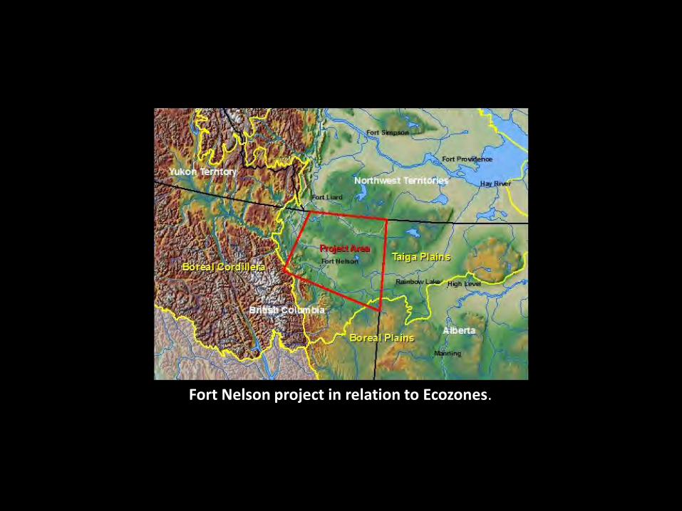
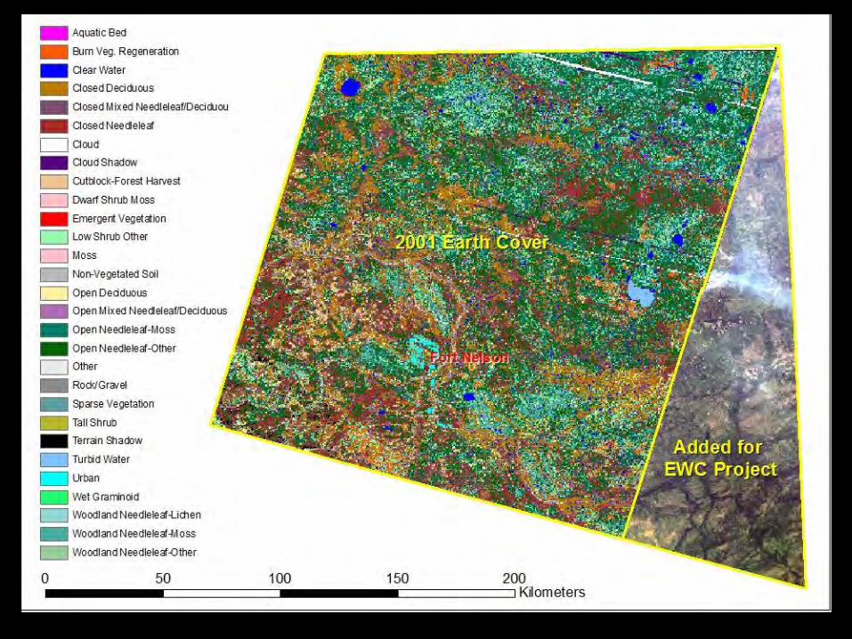
Fort Nelson project in relation to Ecozones.
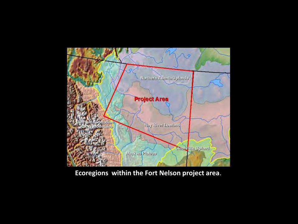
Ecoregions within the Fort Nelson project area.
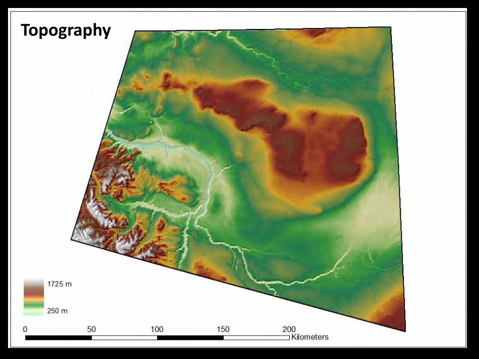
Topography
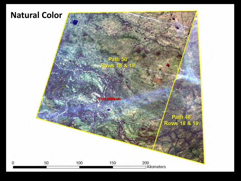
Natural Color
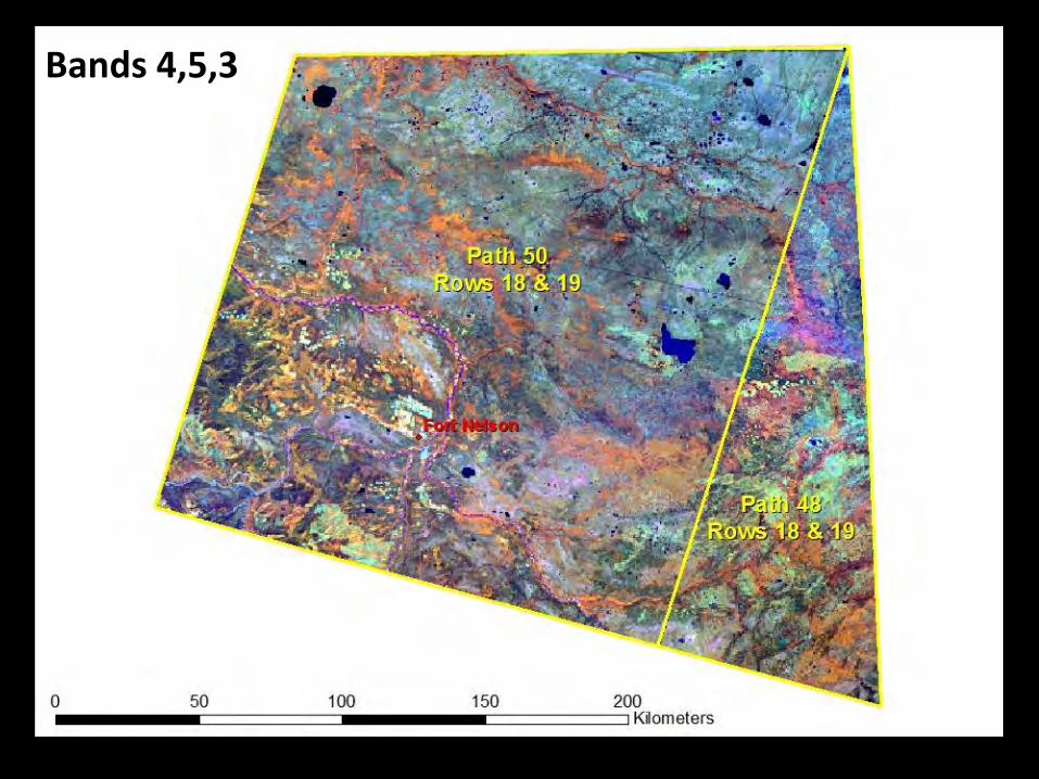
Bands 4,5,3
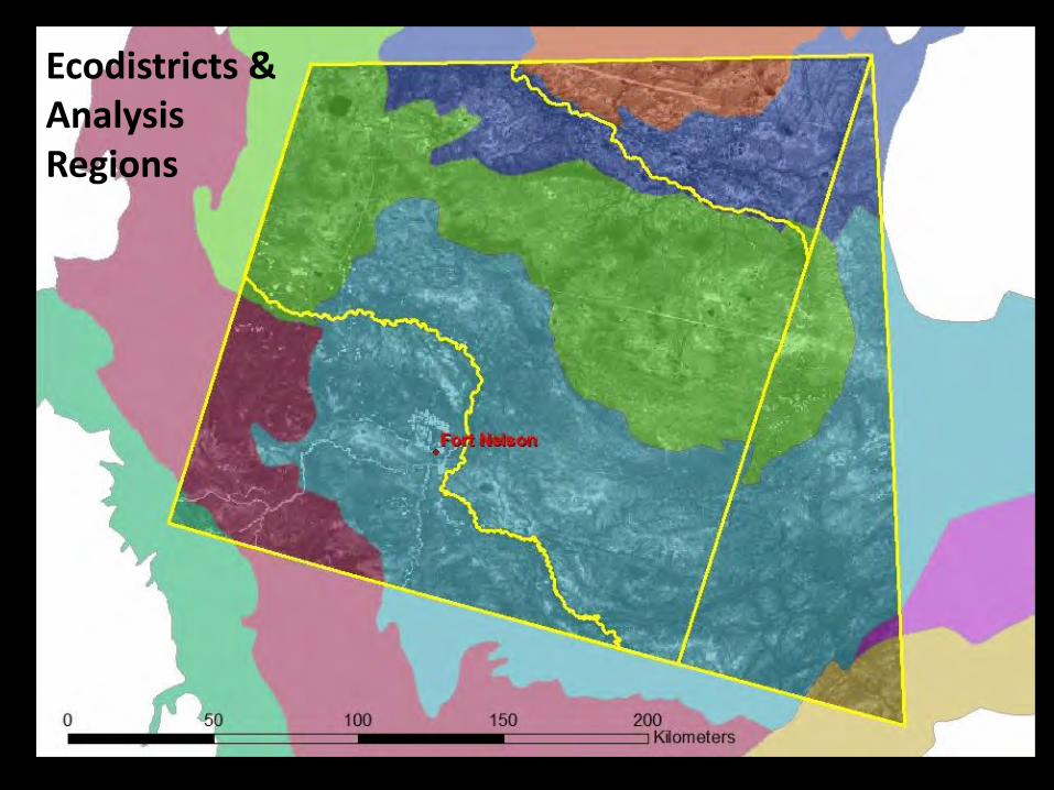
Ecodistricts &Analysis Regions
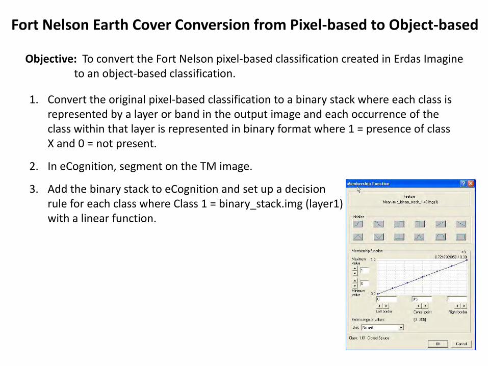
Fort Nelson Earth Cover Conversion from Pixel-based to Object-based
Objective: To convert the Fort Nelson pixel-based classification created in Erdas Imagine to an object-based classification.
1. Convert the original pixel-based classification to a binary stack where each class is represented by a layer or band in the output image and each occurrence of the class within that layer is represented in binary format where 1 = presence of class X and 0 = not present.
2. In eCognition, segment on the TM image.
3. Add the binary stack to eCognition and set up a decision rule for each class where Class 1 = binary_stack.img (layer1) with a linear function.
Fort Nelson Earth Cover Conversion from Pixel-based to Object-based
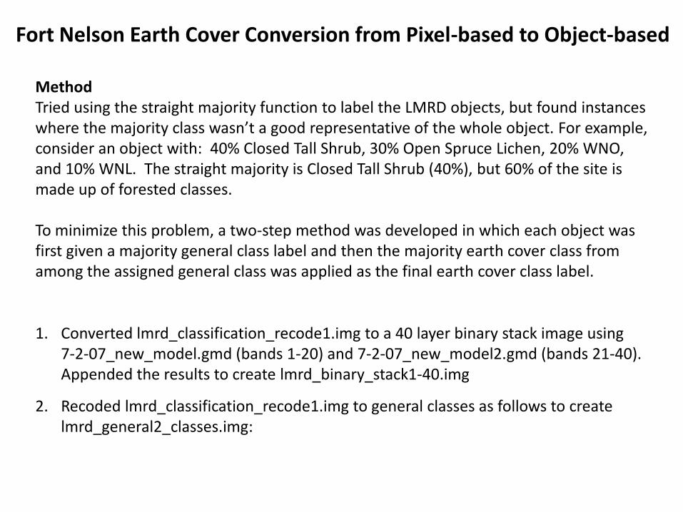
MethodTried using the straight majority function to label the LMRD objects, but found instances where the majority class wasn’t a good representative of the whole object. For example, consider an object with: 40% Closed Tall Shrub, 30% Open Spruce Lichen, 20% WNO, and 10% WNL. The straight majority is Closed Tall Shrub (40%), but 60% of the site is made up of forested classes.
To minimize this problem, a two-step method was developed in which each object was first given a majority general class label and then the majority earth cover class from among the assigned general class was applied as the final earth cover class label.
1. Converted lmrd_classification_recode1.img to a 40 layer binary stack image using 7-2-07_new_model.gmd (bands 1-20) and 7-2-07_new_model2.gmd (bands 21-40). Appended the results to create lmrd_binary_stack1-40.img
2. Recoded lmrd_classification_recode1.img to general classes as follows to create lmrd_general2_classes.img:
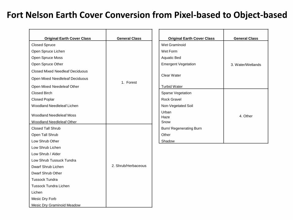
Original Earth Cover Class General Class Original Earth Cover Class General Class
Closed Spruce
1. Forest
Wet Graminoid
3. Water/Wetlands
Open Spruce Lichen Wet Form
Open Spruce Moss Aquatic Bed
Open Spruce Other Emergent Vegetation
Closed Mixed Needleaf DeciduousClear Water
Open Mixed Needleleaf Deciduous
Turbid WaterOpen Mixed Needeleaf Other
Closed Birch Sparse Vegetation
4. Other
Closed Poplar Rock Gravel
Woodland Needleleaf Lichen Non-Vegetated Soil
Woodland Needleleaf MossUrban
Haze
Woodland Needleleaf Other Snow
Closed Tall Shrub
2. Shrub/Herbaceous
Burn/ Regenerating Burn
Open Tall Shrub Other
Low Shrub Other Shadow
Low Shrub Lichen
Low Shrub / Alder
Low Shrub Tussuck Tundra
Dwarf Shrub Lichen
Dwarf Shrub Other
Tussock Tundra
Tussock Tundra Lichen
Lichen
Mesic Dry Forb
Mesic Dry Graminoid Meadow
Fort Nelson Earth Cover Conversion from Pixel-based to Object-based
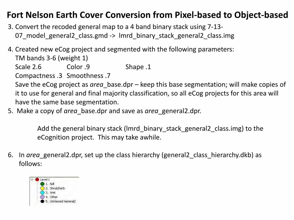
3. Convert the recoded general map to a 4 band binary stack using 7-13-07_model_general2_class.gmd -> lmrd_binary_stack_general2_class.img
4. Created new eCog project and segmented with the following parameters:TM bands 3-6 (weight 1)Scale 2.6 Color .9 Shape .1Compactness .3 Smoothness .7Save the eCog project as area_base.dpr – keep this base segmentation; will make copies of it to use for general and final majority classification, so all eCog projects for this area will have the same base segmentation.
5. Make a copy of area_base.dpr and save as area_general2.dpr.
Add the general binary stack (lmrd_binary_stack_general2_class.img) to the eCognition project. This may take awhile.
6. In area_general2.dpr, set up the class hierarchy (general2_class_hierarchy.dkb) as follows:
Fort Nelson Earth Cover Conversion from Pixel-based to Object-based
Fort Nelson Earth Cover Conversion from Pixel-based to Object-based
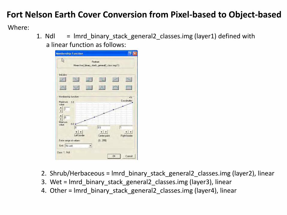
Where:1. Ndl = lmrd_binary_stack_general2_classes.img (layer1) defined with
a linear function as follows:
2. Shrub/Herbaceous = lmrd_binary_stack_general2_classes.img (layer2), linear 3. Wet = lmrd_binary_stack_general2_classes.img (layer3), linear4. Other = lmrd_binary_stack_general2_classes.img (layer4), linear
Fort Nelson Earth Cover Conversion from Pixel-based to Object-based
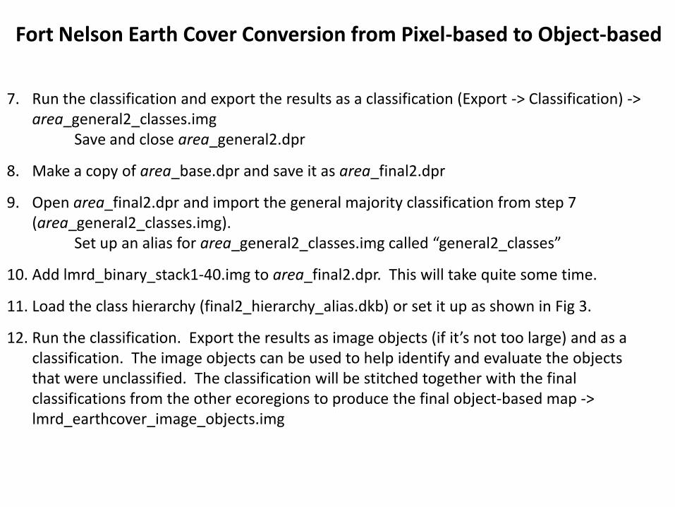
7. Run the classification and export the results as a classification (Export -> Classification) -> area_general2_classes.img
Save and close area_general2.dpr
8. Make a copy of area_base.dpr and save it as area_final2.dpr
9. Open area_final2.dpr and import the general majority classification from step 7 (area_general2_classes.img).
Set up an alias for area_general2_classes.img called “general2_classes”
10. Add lmrd_binary_stack1-40.img to area_final2.dpr. This will take quite some time.
11. Load the class hierarchy (final2_hierarchy_alias.dkb) or set it up as shown in Fig 3.
12. Run the classification. Export the results as image objects (if it’s not too large) and as a classification. The image objects can be used to help identify and evaluate the objects that were unclassified. The classification will be stitched together with the final classifications from the other ecoregions to produce the final object-based map -> lmrd_earthcover_image_objects.img
Fort Nelson Earth Cover Conversion from Pixel-based to Object-based
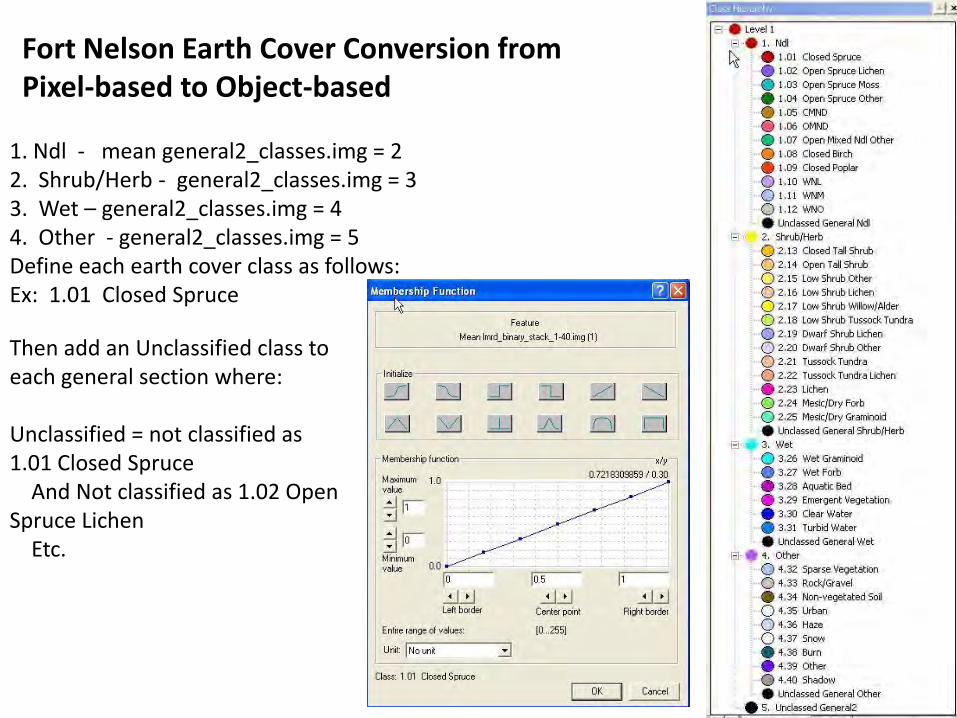
1. Ndl - mean general2_classes.img = 22. Shrub/Herb - general2_classes.img = 33. Wet – general2_classes.img = 44. Other - general2_classes.img = 5Define each earth cover class as follows:Ex: 1.01 Closed Spruce
Then add an Unclassified class to each general section where:
Unclassified = not classified as 1.01 Closed Spruce
And Not classified as 1.02 Open Spruce Lichen
Etc.
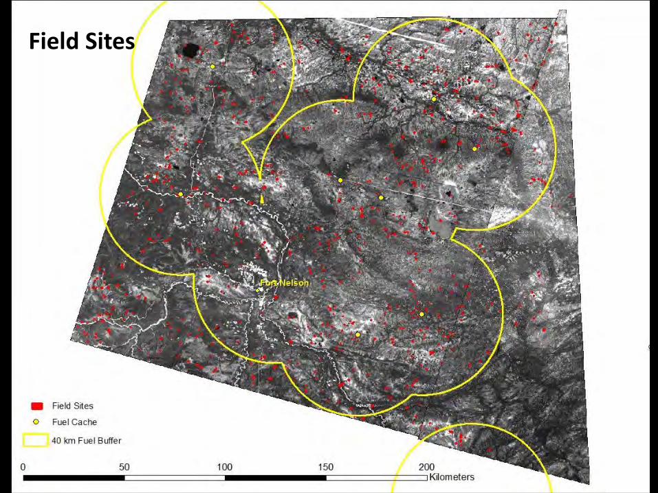
Field Sites
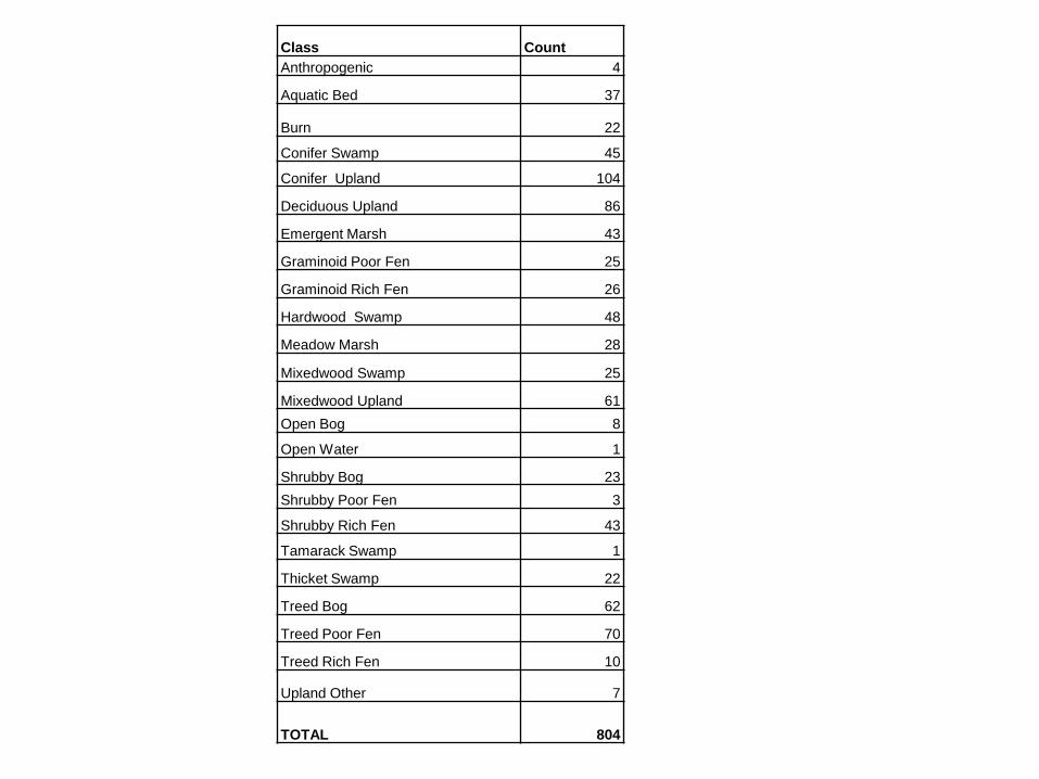
Class Count
Anthropogenic 4
Aquatic Bed 37
Burn 22
Conifer Swamp 45
Conifer Upland 104
Deciduous Upland 86
Emergent Marsh 43
Graminoid Poor Fen 25
Graminoid Rich Fen 26
Hardwood Swamp 48
Meadow Marsh 28
Mixedwood Swamp 25
Mixedwood Upland 61
Open Bog 8
Open Water 1
Shrubby Bog 23
Shrubby Poor Fen 3
Shrubby Rich Fen 43
Tamarack Swamp 1
Thicket Swamp 22
Treed Bog 62
Treed Poor Fen 70
Treed Rich Fen 10
Upland Other 7
TOTAL 804
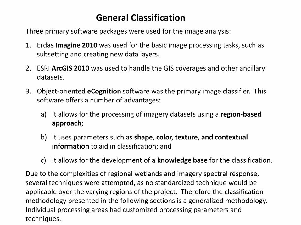
Three primary software packages were used for the image analysis:
1. Erdas Imagine 2010 was used for the basic image processing tasks, such as subsetting and creating new data layers.
2. ESRI ArcGIS 2010 was used to handle the GIS coverages and other ancillary datasets.
3. Object-oriented eCognition software was the primary image classifier. This software offers a number of advantages:
a) It allows for the processing of imagery datasets using a region-based approach;
b) It uses parameters such as shape, color, texture, and contextual information to aid in classification; and
c) It allows for the development of a knowledge base for the classification.
General Classification
Due to the complexities of regional wetlands and imagery spectral response, several techniques were attempted, as no standardized technique would be applicable over the varying regions of the project. Therefore the classification methodology presented in the following sections is a generalized methodology. Individual processing areas had customized processing parameters and techniques.
General Classification
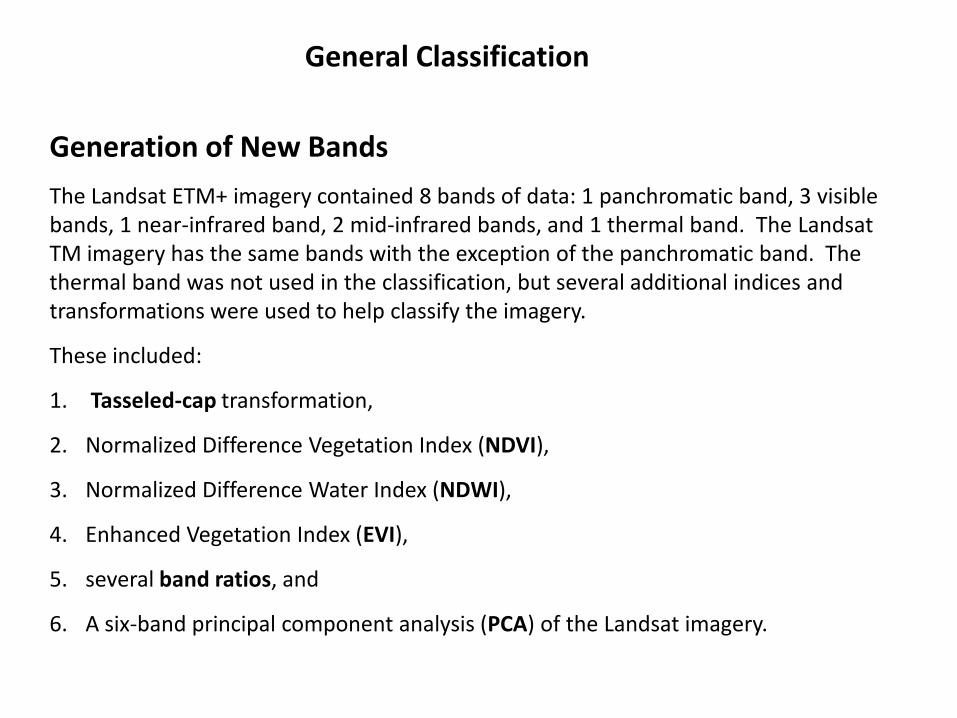
Generation of New Bands
The Landsat ETM+ imagery contained 8 bands of data: 1 panchromatic band, 3 visible bands, 1 near-infrared band, 2 mid-infrared bands, and 1 thermal band. The LandsatTM imagery has the same bands with the exception of the panchromatic band. The thermal band was not used in the classification, but several additional indices and transformations were used to help classify the imagery.
These included:
1. Tasseled-cap transformation,
2. Normalized Difference Vegetation Index (NDVI),
3. Normalized Difference Water Index (NDWI),
4. Enhanced Vegetation Index (EVI),
5. several band ratios, and
6. A six-band principal component analysis (PCA) of the Landsat imagery.
Segmentation
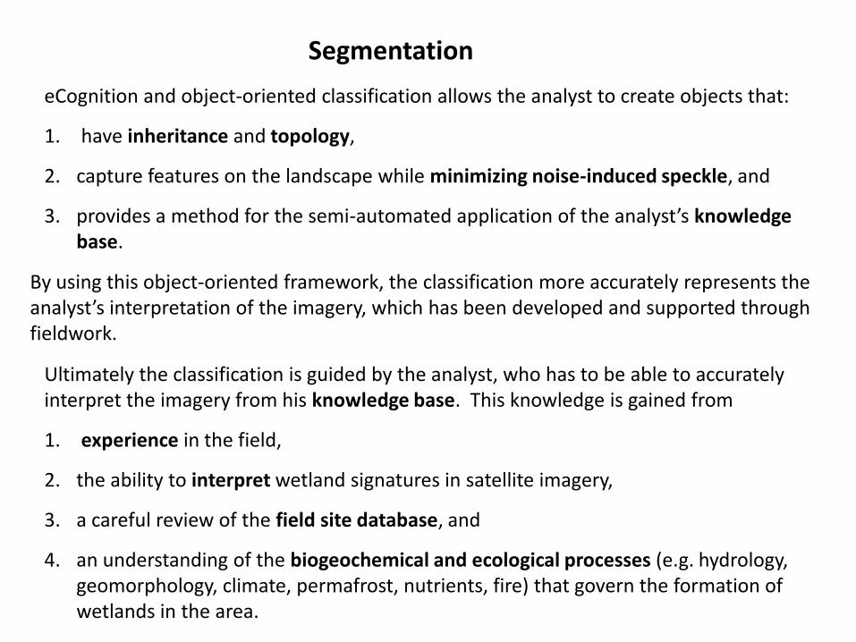
eCognition and object-oriented classification allows the analyst to create objects that:
1. have inheritance and topology,
2. capture features on the landscape while minimizing noise-induced speckle, and
3. provides a method for the semi-automated application of the analyst’s knowledge base.
By using this object-oriented framework, the classification more accurately represents the analyst’s interpretation of the imagery, which has been developed and supported through fieldwork.
Ultimately the classification is guided by the analyst, who has to be able to accurately interpret the imagery from his knowledge base. This knowledge is gained from
1. experience in the field,
2. the ability to interpret wetland signatures in satellite imagery,
3. a careful review of the field site database, and
4. an understanding of the biogeochemical and ecological processes (e.g. hydrology, geomorphology, climate, permafrost, nutrients, fire) that govern the formation of wetlands in the area.
Segmentation
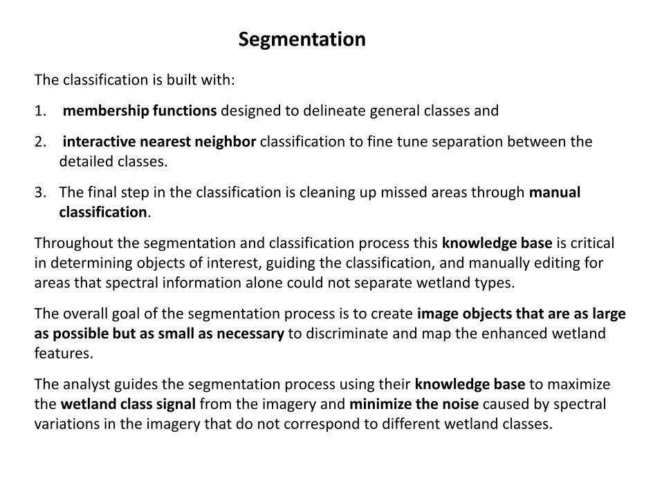
The classification is built with:
1. membership functions designed to delineate general classes and
2. interactive nearest neighbor classification to fine tune separation between the detailed classes.
3. The final step in the classification is cleaning up missed areas through manual classification.
Throughout the segmentation and classification process this knowledge base is critical in determining objects of interest, guiding the classification, and manually editing for areas that spectral information alone could not separate wetland types.
The overall goal of the segmentation process is to create image objects that are as large as possible but as small as necessary to discriminate and map the enhanced wetland features.
The analyst guides the segmentation process using their knowledge base to maximize the wetland class signal from the imagery and minimize the noise caused by spectral variations in the imagery that do not correspond to different wetland classes.
Segmentation
For example, an image object needs to be thin and narrow to pull out a faint drainage feature from the imagery.
At the same time, some image objects also need to be large and round for homogenous areas.
Within the imagery, a large area may be only one wetland class but it’s spectrally signature will vary widely based on slight variations in shrub understory, presence of water, or amount of litter present. This spectral variation that doesn’t correspond to a change in wetland class is noise. In a pixel-based process, this noise can greatly affect the classification and produce speckle that does not correlate to wetland classes.
With object-based processing, the analyst uses spatial, spectral, and contextual information to derive the types of objects that will provide the building blocks for the classification. The quality of these objects is very important for the classification.
If the boundaries of the image objects are not representative of the shapes of the wetland areas (e.g. narrow drainage features), then classification of the wetland areas will in turn be difficult.
At the same time, objects need to be large in homogenous areas. The objects are able to filter out the spectral noise that doesn’t correspond to change in wetland classes.
So the image objects work to maximize the capture of the signal and reduce errors of omission and they work to minimize the noise of the imagery and reduce errors of commission.
Segmentation
Segmentation
For each processing area,
1. the six-band ETM+ image subset, excluding the panchromatic and thermal bands, was added to an eCognition project along with
2. the first three bands of the principal components image and
3. the tasseled-cap brightness/greenness/wetness image.
The imagery was then segmented at scale 2.25. Scale 2.25 was chosen because the resulting image objects provided good discrimination of spectral differences between and within enhanced wetland types, yet was not so fine as to result in a high proportion of single pixel objects. Scale 2.25 has been used in other DU projects when only TM imagery was available.
Segmentation
1. Input bands for the segmentation included the six bands of the ETM+ imagery and additional bands that showed clear separation of the objects being classified in the imagery.
2. In the Taiga Plains where the spectral separation between wetland classes is very subtle, introducing additional bands helps to more accurately delineate the image objects along wetland boundaries.
3. The characteristics of the input bands greatly affect both the image objects size and shape.
4. The following graphic shows an example of the same area segmented with the same segmentation parameters at a scale of 50. For illustrative purposes, one is segmented using only the near-infrared band as input and the other is segmented using only the PCA band 1. The PCA band 1 segmentation produced smaller objects that delineated the boundaries of the peatland with finer detail. Emphasizing band 4 for peatland delineation would not effectively extract the general peatland class from the surrounding landcover.
5. Different input bands and weights were used specific to the wetland being extracted from the imagery in order to obtain the ideal image object size and shape.
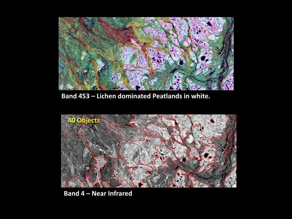
40 Objects
Band 453 – Lichen dominated Peatlands in white.
Band 4 – Near Infrared
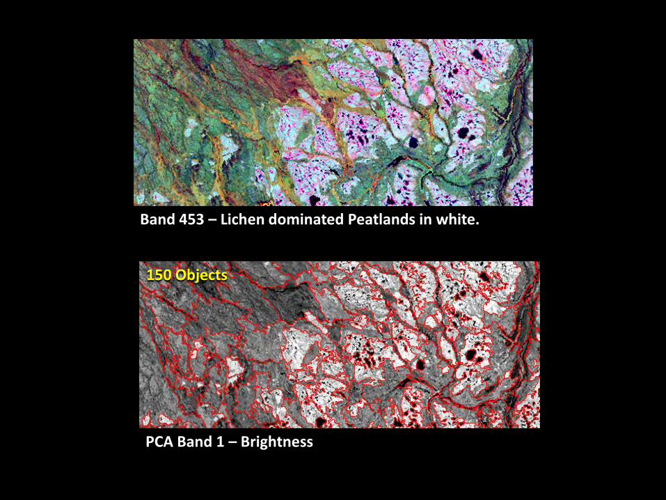
150 Objects
Band 453 – Lichen dominated Peatlands in white.
PCA Band 1 – Brightness
Segmentation
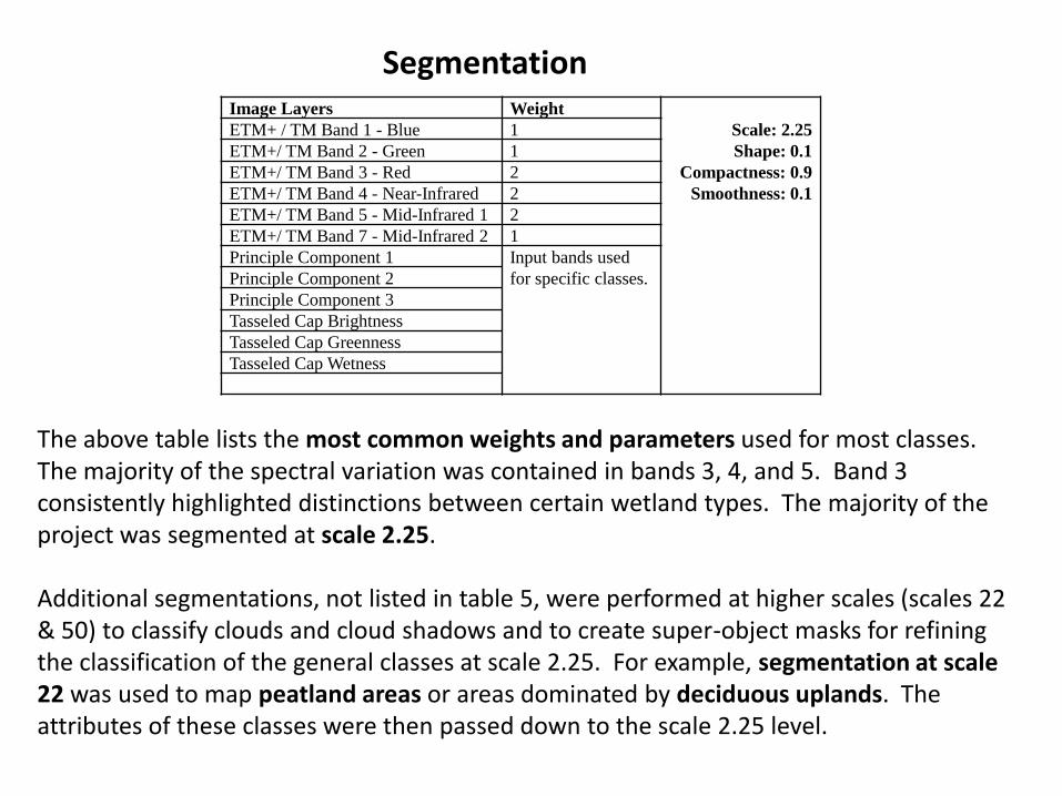
The above table lists the most common weights and parameters used for most classes. The majority of the spectral variation was contained in bands 3, 4, and 5. Band 3 consistently highlighted distinctions between certain wetland types. The majority of the project was segmented at scale 2.25.
Additional segmentations, not listed in table 5, were performed at higher scales (scales 22 & 50) to classify clouds and cloud shadows and to create super-object masks for refining the classification of the general classes at scale 2.25. For example, segmentation at scale 22 was used to map peatland areas or areas dominated by deciduous uplands. The attributes of these classes were then passed down to the scale 2.25 level.
Image Layers Weight
Scale: 2.25
Shape: 0.1
Compactness: 0.9
Smoothness: 0.1
ETM+ / TM Band 1 - Blue 1
ETM+/ TM Band 2 - Green 1
ETM+/ TM Band 3 - Red 2
ETM+/ TM Band 4 - Near-Infrared 2
ETM+/ TM Band 5 - Mid-Infrared 1 2
ETM+/ TM Band 7 - Mid-Infrared 2 1
Principle Component 1 Input bands used
for specific classes.Principle Component 2
Principle Component 3
Tasseled Cap Brightness
Tasseled Cap Greenness
Tasseled Cap Wetness
Classification
The classification scheme is based on the “Enhanced Wetland Classification for the Boreal Plains” (Smith et al., 2007). For an example of its application see “A User’s Guide to the Enhanced Wetland Classification for the Al-Pac Boreal Conservation Project” (Smith 2006).
This Enhanced Wetland Classification in the Taiga Plains is a modification of the Boreal Plains classification scheme. The Taiga Plains in general has lower nutrient levels and more open canopies. The same wetland classes in the Boreal Plains will be expressed differently in the Taiga Plains.
For example, Larix laricina (Tamarack) is a primary wetland indicator tree species found in fens and swamps of the Boreal Plains ecozone, but it is not a dominant species in fens and swamps of the Taiga Plains.
Climate-driven processes such as permafrost formation also changes the expression of the wetland types and their position in the landscape.
Treed Bog
ShrubbyBog
OpenBog
TreedPoor Fen
ShrubbyPoor Fen
Graminoid Poor Fen
EmergentMarsh
MeadowMarsh
Treed Rich Fen
Shrubby Rich Fen
Graminoid Rich Fen
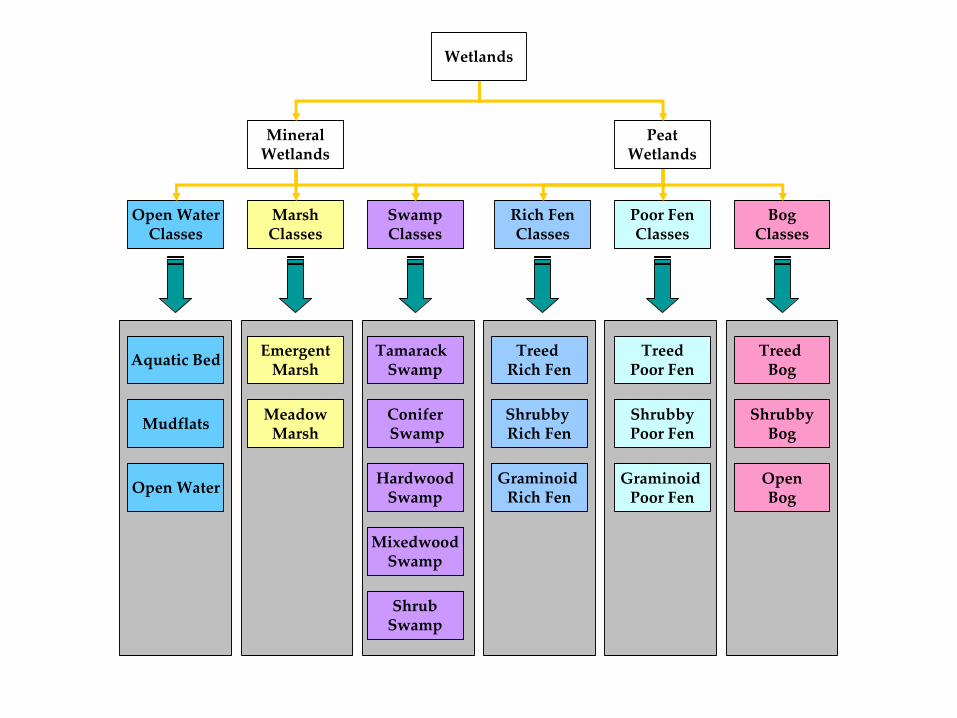
Open WaterClasses
HardwoodSwamp
ConiferSwamp
Tamarack Swamp
ShrubSwamp
MixedwoodSwamp
SwampClasses
Open Water
Mudflats
Aquatic Bed
MarshClasses
Rich FenClasses
Poor FenClasses
BogClasses
MineralWetlands
PeatWetlands
Wetlands
Boreal Plains Boreal Plains EcozoneEcozone Wetland Wetland Class HierarchyClass Hierarchy
Classification
The first step in the classification procedure is an initial segmentation that aims to delineate general wetland classes from the imagery.
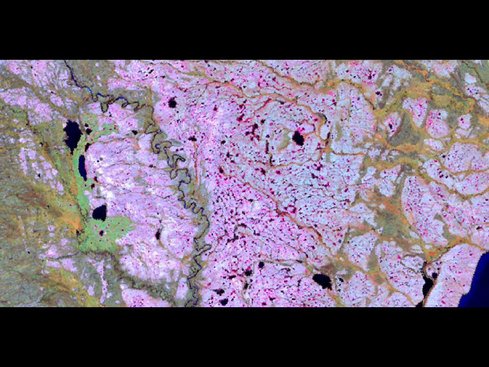
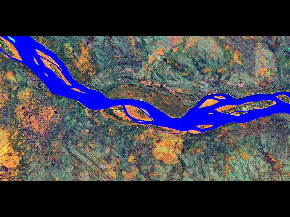
The Basin general class is usually the first class that is delineated. The Basin general class contains the detailed classes of Open Water, Aquatic Bed, and Emergent Marsh. This segmentation is designed to separate the Basin class from the rest of the imagery, because of the large amount of spectral overlaps between wetland signatures and many upland signatures in the imagery.
An initial classification is performed with membership functions, which can be as simple as a threshold placed on a single band or it can be very complicated with many thresholds and conditional statements joined in a logical structure. Membership functions are also used to access the object’s topology and inheritance. The initial classification highlights weak areas in the initial segmentation where features where not adequately captured.
The project is resegmented with parameters adjusted to capture features that were initially missed in the first segmentation. The image objects are then classified using membership functions with a secondary classification.
Classification
Once the general classes are defined, the underlying detailed classes were separated using an interactive nearest neighbor classification.
The segmentation parameters are designed now to separate within-class subtle variations associated with changes in the detailed classes.
Field sites are initially used in the nearest neighbor classification. But the analyst guides the overall classification by selecting visually interpreted training sites to augment the process. By visual interpretation, the analyst can shape the classification in a semi-automated fashion.
Membership functions are also used within the nearest neighbor classification but are primarily used to spatially limit the application of different training sites on the image.
The development of the Enhanced Wetland Classification is a combination of elements used in the earth cover classification and then the splitting of the final detailed earth cover classes into their wetland subclasses (following table). The Basin general class is used in dividing different earth cover classes into their respective wetland subclasses. The final detailed classes are segmented to separate each of the wetland classes held within each of the earth cover class.
Although parts of the earth cover classification are reused in the enhanced wetland class, the majority of the processing for the enhanced wetlands classification is taking the earth cover classes and breaking them into their corresponding wetland subclasses (followingtable). 27 earth cover classes were split into as many as 4 wetland classes each, totaling 60 classes. The techniques for each of these splits were unique to the wetland classification and required application of the analyst’s knowledge base via membership functions. Not only was spectral information used but also features such as standard deviation of superobjects, relative distance, position in the landscape, and membership to an ecodistrict. These 60 classes were then grouped into 26 classes for the Enhanced Wetlands classification. The Enhanced Wetlands Classes were then grouped together to form the CWWS classes. A general upland and wetland class were also studied for landscape position and accuracy assessment since this can be the most difficult distinction to make.
Classification
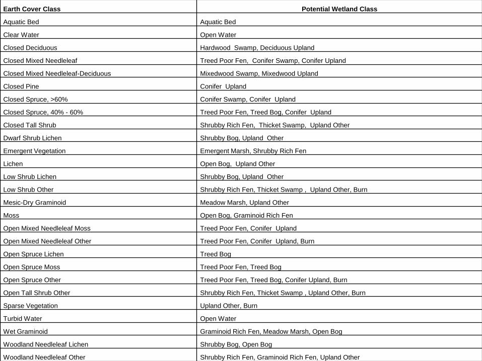
Earth Cover Class Potential Wetland Class
Aquatic Bed Aquatic Bed
Clear Water Open Water
Closed Deciduous Hardwood Swamp, Deciduous Upland
Closed Mixed Needleleaf Treed Poor Fen, Conifer Swamp, Conifer Upland
Closed Mixed Needleleaf-Deciduous Mixedwood Swamp, Mixedwood Upland
Closed Pine Conifer Upland
Closed Spruce, >60% Conifer Swamp, Conifer Upland
Closed Spruce, 40% - 60% Treed Poor Fen, Treed Bog, Conifer Upland
Closed Tall Shrub Shrubby Rich Fen, Thicket Swamp, Upland Other
Dwarf Shrub Lichen Shrubby Bog, Upland Other
Emergent Vegetation Emergent Marsh, Shrubby Rich Fen
Lichen Open Bog, Upland Other
Low Shrub Lichen Shrubby Bog, Upland Other
Low Shrub Other Shrubby Rich Fen, Thicket Swamp , Upland Other, Burn
Mesic-Dry Graminoid Meadow Marsh, Upland Other
Moss Open Bog, Graminoid Rich Fen
Open Mixed Needleleaf Moss Treed Poor Fen, Conifer Upland
Open Mixed Needleleaf Other Treed Poor Fen, Conifer Upland, Burn
Open Spruce Lichen Treed Bog
Open Spruce Moss Treed Poor Fen, Treed Bog
Open Spruce Other Treed Poor Fen, Treed Bog, Conifer Upland, Burn
Open Tall Shrub Other Shrubby Rich Fen, Thicket Swamp , Upland Other, Burn
Sparse Vegetation Upland Other, Burn
Turbid Water Open Water
Wet Graminoid Graminoid Rich Fen, Meadow Marsh, Open Bog
Woodland Needleleaf Lichen Shrubby Bog, Open Bog
Woodland Needleleaf Other Shrubby Rich Fen, Graminoid Rich Fen, Upland Other
Classification
Many attempts were made to use the DEM but the 30m resolution was too coarse to make any detailed analysis of wetlands. Wetlands often occur in flat areas, where subtle changes in elevation result in very different wetland types, and the vertical resolution of the DEM was not sufficient to discriminate wetland areas. The DEM therefore was used only to make broad distinctions between mountains and plains.
For this project, the final steps of the classification process were to edit the confused classes remaining after the classification process and to make final edits in areas that still had classification errors. Editing of classification errors was a process of comparing the classified image to the raw satellite image, field photos, and notes on field maps to identify errors remaining in the classification. These errors were then corrected by manually changing the class value for the image objects that were classified in error to their correct class value. This step is critical to the accurate mapping of wetland areas, which vary greatly across the study area, exhibit a wide range of spectral variation, and often occur in high percentages of the land area. Application of the analyst’s knowledge base via manual editing is often necessary to accurately delineate the more challenging wetland types/areas.
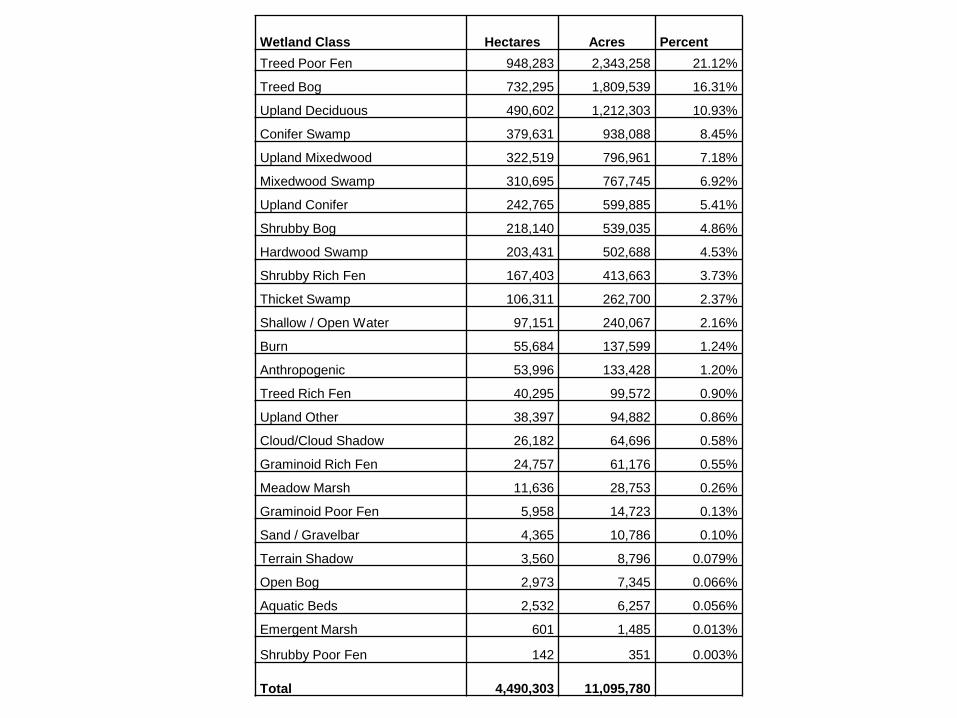
Wetland Class Hectares Acres Percent
Treed Poor Fen 948,283 2,343,258 21.12%
Treed Bog 732,295 1,809,539 16.31%
Upland Deciduous 490,602 1,212,303 10.93%
Conifer Swamp 379,631 938,088 8.45%
Upland Mixedwood 322,519 796,961 7.18%
Mixedwood Swamp 310,695 767,745 6.92%
Upland Conifer 242,765 599,885 5.41%
Shrubby Bog 218,140 539,035 4.86%
Hardwood Swamp 203,431 502,688 4.53%
Shrubby Rich Fen 167,403 413,663 3.73%
Thicket Swamp 106,311 262,700 2.37%
Shallow / Open Water 97,151 240,067 2.16%
Burn 55,684 137,599 1.24%
Anthropogenic 53,996 133,428 1.20%
Treed Rich Fen 40,295 99,572 0.90%
Upland Other 38,397 94,882 0.86%
Cloud/Cloud Shadow 26,182 64,696 0.58%
Graminoid Rich Fen 24,757 61,176 0.55%
Meadow Marsh 11,636 28,753 0.26%
Graminoid Poor Fen 5,958 14,723 0.13%
Sand / Gravelbar 4,365 10,786 0.10%
Terrain Shadow 3,560 8,796 0.079%
Open Bog 2,973 7,345 0.066%
Aquatic Beds 2,532 6,257 0.056%
Emergent Marsh 601 1,485 0.013%
Shrubby Poor Fen 142 351 0.003%
Total 4,490,303 11,095,780
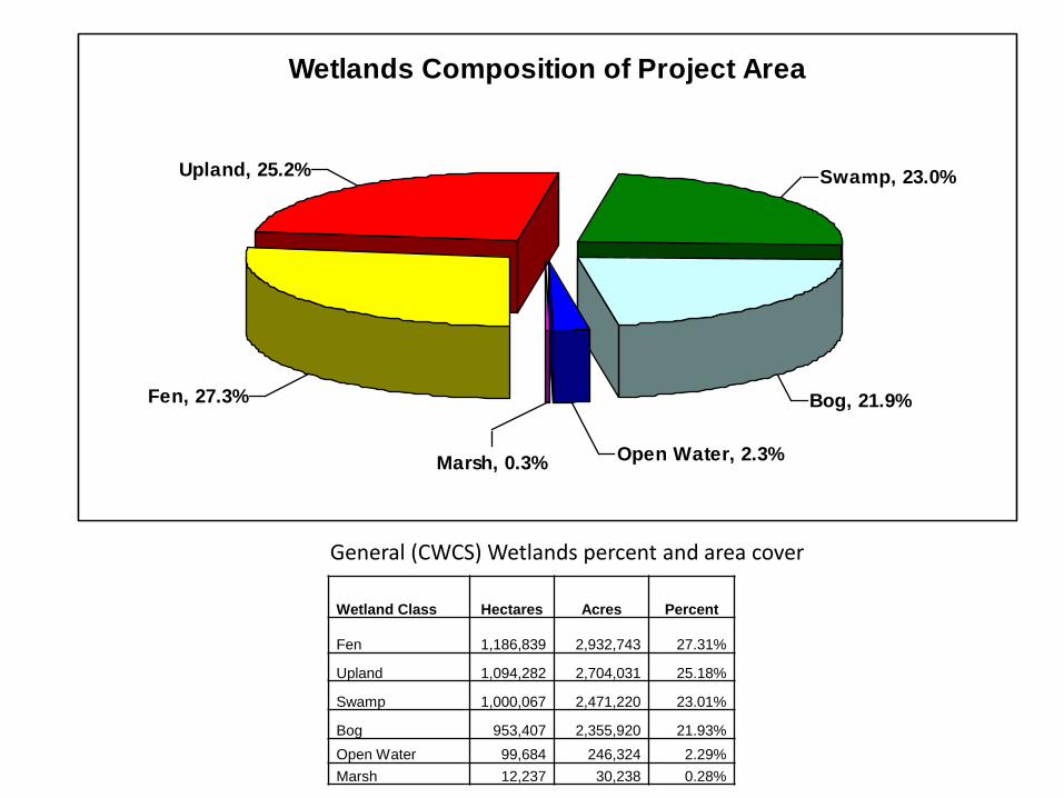
Wetland Class Hectares Acres Percent
Fen 1,186,839 2,932,743 27.31%
Upland 1,094,282 2,704,031 25.18%
Swamp 1,000,067 2,471,220 23.01%
Bog 953,407 2,355,920 21.93%
Open Water 99,684 246,324 2.29%
Marsh 12,237 30,238 0.28%
Wetlands Composition of Project Area
Bog, 21.9%
Swamp, 23.0%Upland, 25.2%
Fen, 27.3%
Marsh, 0.3% Open Water, 2.3%
General (CWCS) Wetlands percent and area cover
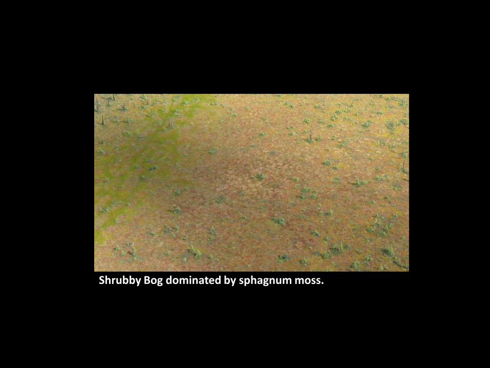
Shrubby Bog dominated by sphagnum moss.
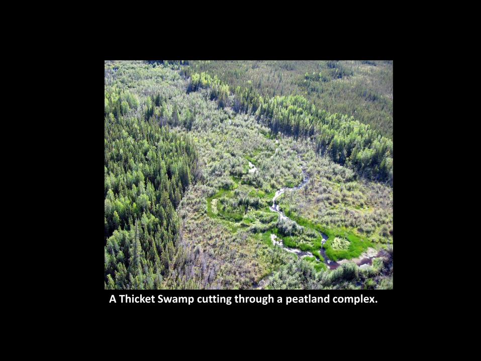
A Thicket Swamp cutting through a peatland complex.
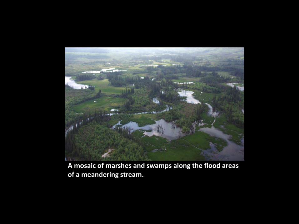
A mosaic of marshes and swamps along the flood areas of a meandering stream.
Class
Up
Con
Up
Decid
Up
Mix TBOG
OBOG/
SBOG TrPF
GrPF/
ShPF ShRF GrRF AQBD EMSH MMSH CSWP HSWP MSWP TSWP Total User's
UpCon 19 1 1 21 90.5
UpDecid 26 26 100.0
UpMix 1 17 18 94.4
TBOG 14 1 2 17 82.4
OBOG/
SBOG 2 9 1 12 75.0
TrPF 3 1 17 2 23 73.9
GrPF/
ShPF 9 1 10 80.0
ShRF 11 11 100.0
GrRF 4 4 100.0
OWTR 5 5 0.0
AQBD 9 9 100.0
SBAR 1 1 0.0
EMSH 2 2 100.0
MMSH 6 6 100.0
CSWP 1 11 12 91.7
HSWP 1 15 1 1 18 83.3
MSWP 5 1 6 83.3
TSWP 1 3 4 8 50.0
Total 24 26 18 17 10 20 9 13 5 10 7 6 13 15 9 7 209
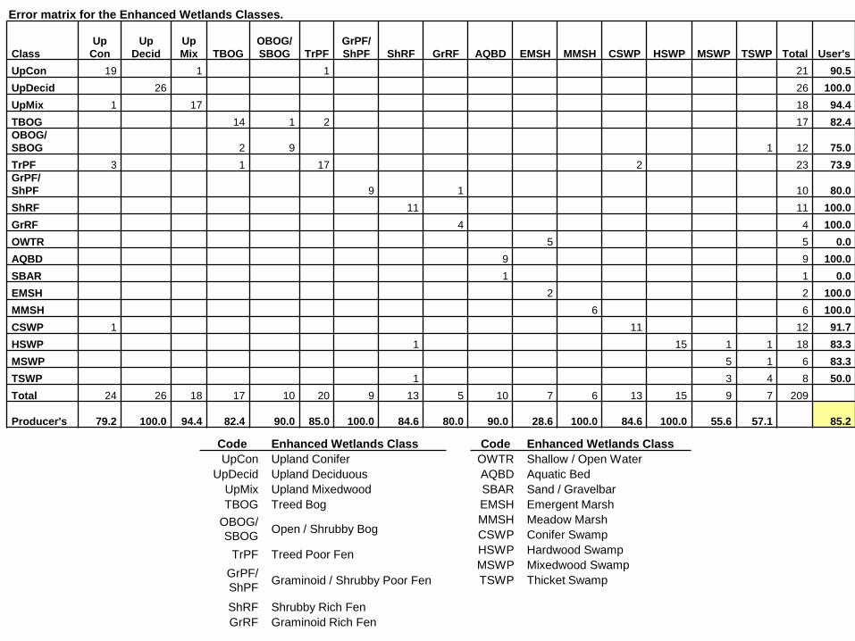
Producer's 79.2 100.0 94.4 82.4 90.0 85.0 100.0 84.6 80.0 90.0 28.6 100.0 84.6 100.0 55.6 57.1 85.2
Code Enhanced Wetlands Class
UpCon Upland Conifer
UpDecid Upland Deciduous
UpMix Upland Mixedwood
TBOG Treed Bog
OBOG/
SBOGOpen / Shrubby Bog
TrPF Treed Poor Fen
GrPF/
ShPFGraminoid / Shrubby Poor Fen
ShRF Shrubby Rich Fen
GrRF Graminoid Rich Fen
Code Enhanced Wetlands Class
OWTR Shallow / Open Water
AQBD Aquatic Bed
SBAR Sand / Gravelbar
EMSH Emergent Marsh
MMSH Meadow Marsh
CSWP Conifer Swamp
HSWP Hardwood Swamp
MSWP Mixedwood Swamp
TSWP Thicket Swamp
Error matrix for the Enhanced Wetlands Classes.
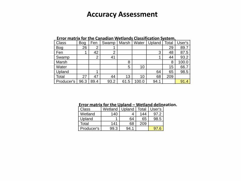
Class Bog Fen Swamp Marsh Water Upland Total User's
Bog 26 2 1 29 89.7
Fen 1 42 2 3 48 87.5
Swamp 2 41 1 44 93.2
Marsh 8 8 100.0
Water 5 10 15 66.7
Upland 1 64 65 98.5
Total 27 47 44 13 10 68 209
Producer's 96.3 89.4 93.2 61.5 100.0 94.1 91.4
Class Wetland Upland Total User's
Wetland 140 4 144 97.2
Upland 1 64 65 98.5
Total 141 68 209
Producer's 99.3 94.1 97.6
Accuracy Assessment
Error matrix for the Canadian Wetlands Classification System.
Error matrix for the Upland – Wetland delineation.
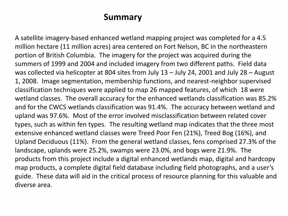
Summary
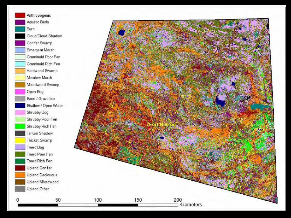
A satellite imagery-based enhanced wetland mapping project was completed for a 4.5 million hectare (11 million acres) area centered on Fort Nelson, BC in the northeastern portion of British Columbia. The imagery for the project was acquired during the summers of 1999 and 2004 and included imagery from two different paths. Field data was collected via helicopter at 804 sites from July 13 – July 24, 2001 and July 28 – August 1, 2008. Image segmentation, membership functions, and nearest-neighbor supervised classification techniques were applied to map 26 mapped features, of which 18 were wetland classes. The overall accuracy for the enhanced wetlands classification was 85.2% and for the CWCS wetlands classification was 91.4%. The accuracy between wetland and upland was 97.6%. Most of the error involved misclassification between related cover types, such as within fen types. The resulting wetland map indicates that the three most extensive enhanced wetland classes were Treed Poor Fen (21%), Treed Bog (16%), and Upland Deciduous (11%). From the general wetland classes, fens comprised 27.3% of the landscape, uplands were 25.2%, swamps were 23.0%, and bogs were 21.9%. The products from this project include a digital enhanced wetlands map, digital and hardcopy map products, a complete digital field database including field photographs, and a user’s guide. These data will aid in the critical process of resource planning for this valuable and diverse area.
Partners
Questions ?