An Effective Dynamic Programming Algorithm for the

Minimum-Cost Maximal Knapsack Packing

Fabio Furini∗1, Ivana Ljubic†2, and Markus Sinnl‡3

1PSL, Universite Paris-Dauphine, France2ESSEC Business School of Paris, France

3Department of Statistics and Operations Research, University of Vienna, Austria

Abstract

Given a set of n items with profits and weights and a knapsack capacity C, we study the problem of

finding a maximal knapsack packing that minimizes the profit of selected items. We propose for the first

time an effective dynamic programming (DP) algorithm which has O(nC) time complexity and O(n+C)

space complexity. We demonstrate the equivalence between this problem and the problem of finding

a minimal knapsack cover that maximizes the profit of selected items. In an extensive computational

study on a large and diverse set of benchmark instances, we demonstrate that the new DP algorithm

outperforms the use of a state-of-the-art commercial mixed integer programming (MIP) solver applied

to the two best-performing MIP models from the literature.

1. Introduction

One of the most famous and the most studied problems in combinatorial optimization is the classical Knap-

sack Problem (KP) which is defined as follows: Given an knapsack capacity C > 0 and a set I = {1, . . . , n}of items, with profits pi ≥ 0 and weights wi ≥ 0, KP asks for a maximum profit subset of items whose total

weight does not exceed the capacity. The problem can be formulated using the following Integer Linear

Program (ILP):

max

{∑i∈I

pixi :∑i∈I

wixi ≤ C, xi ∈ {0, 1}, i ∈ I

}(1)

where each variable xi takes value 1 if and only if item i is inserted in the knapsack. Without loss of generality

we can assume that all input parameters have integer values. In the following, we will refer to (I, p, w,C)

as a knapsack instance. KP is NP-hard, but it is well-known that fairly large instances can be solved to

∗fabio.furini@dauphine.fr†ivana.ljubic@essec.edu‡markus.sinnl@univie.ac.at

1

optimality within short computing times (see, e.g., [14, 17, 16] for comprehensive surveys on applications

and variants of KP).

Optimization problems related to KP search for solutions satisfying one of the following two properties:

Definition 1 (Maximal Knapsack Packing). Given a knapsack instance (I, p, w,C), a packing P is a subset

of items which does not exceed the capacity C, i.e.,∑i∈P wi ≤ C. A packing P is called maximal, iff P∪{i}

is not a packing for any i 6∈ P.

Definition 2 (Minimal Knapsack Cover). Given a knapsack instance (I, p, w,C), a cover C is a subset of

items which exceeds the capacity C, i.e.,∑c∈C wc ≥ C. A cover C is called minimal, iff C \{i} is not a cover

for any i ∈ C.

In this article we study weighted versions of the knapsack covering and knapsack packing problems which

are defined below.

Definition 3 (Minimum-Cost Maximal Knapsack Packing (MCMKP)). Given a knapsack instance (I, p,

w,C), the goal of the MCMKP is to find a maximal knapsack packing S∗ ⊂ I that minimizes the profit of

selected items, i.e.:

S∗ = arg minS⊂I{∑i∈S

pi |∑i∈S

wi ≤ C and∑i∈S

wi + wj > C, ∀j 6∈ S}.

Definition 4 (Maximum-Profit Minimal Knapsack Cover (MPMKC)). Given a knapsack instance (I, p, w,

C), the goal of the MPMKC is to find a minimal knapsack cover S∗ ⊆ I that maximizes the profit, i.e.:

S∗ = arg maxS⊂I{∑i∈S

pi |∑i∈S

wi ≥ C and∑

i∈S\{j}

wi < C, ∀j ∈ S}.

In both, MCMKP and MPMKC, we assume that the problem instance (I, p, w,C) is non-trivial, i.e., the

corresponding optimal solution S∗ is a proper subset of I.

In the classical KP, one tries to pack the knapsack while maximizing the (non-negative) profit of selected

items, hence, every optimal KP solution trivially satisfies the maximal knapsack packing property. On the

contrary, the objective function of the MCMKP goes in the opposite direction – one searches for a subset of

items to pack in the knapsack, while minimizing the profit of selected items. Hence, solving the standard

KP in which the profit-maximization objective is replaced by profit-minimization results in a trivial (empty)

solution. This is why the maximal packing property has to be explicitly imposed, when searching for an

optimal MCMKP solution.

The MCMKP models applications related to scheduling jobs on a single machine with common arrival

times and a common deadline. The problem consists of selecting a subset of jobs to schedule (before the

given deadline) and accordingly the order in which the jobs are scheduled becomes irrelevant. The set I

refers to all possible jobs, job durations are given as wi and pi is the cost for executing job i, i ∈ I. The

common deadline C corresponds to the capacity of the knapsack. The goal is to minimize the cost for

executing scheduled jobs while at the same time ensuring that the maximal subset of jobs is scheduled (i.e.,

a maximal packing is preserved). Consequently, the scheduling task boils down to solving MCMKP. The

problem has been called the Lazy Bureaucrat Problem (LBP) (see, e.g. [11]), motivated by the special case

2

in which pi = wi, for all i ∈ I. We deliberately refrain from this name since in this article we study a more

general setting in which no correlation is assumed to exist between the item profits and item weights.

Similarly, in case of MPMKC, the goal is to maximize the profit of scheduled jobs while ensuring that

a minimal possible subset of jobs exceeding the deadline is scheduled (i.e., to preserve a minimal cover).

The MPMKC problem has been called the Greedy Boss Problem in [11], but again, since this name is also

motivated by the setting pi = wi, for all i ∈ I, we will not use it in the remainder of this article.

Literature Overview The MCMKP problem has been introduced in [1] where it was shown that a more

general problem variant with individual arrival times and deadlines is NP-hard. Following this seminal

work, the problem has been extensively studied in the Computer Science literature and results concerning

the problem complexity of special classes and approximation algorithms have been presented ([8, 11, 13]).

On the contrary, concerning the development of exact methods, the problem has been tackled only in a

recent preliminary study [7].

Depending on the coefficients pi of the objective function, the following special cases are known in the

(scheduling) literature:

• min-number-of-jobs: In this case, pi = 1 for all i ∈ I and the goal is to minimize the number of

scheduled jobs. By reduction from the subset-sum problem, it has been shown in [8] that this problem

variant is weakly NP-hard.

• min-time-spent: This variant corresponds to the problem in which pi = wi for all i ∈ I. Since job

profits are equal to job durations, this explains the motivation for calling the problem LBP, i.e., the

goal of the “lazy employee” is to go home as early as possible, while having an excuse that there is

no more time left to start a new job. This variant is also equivalent to the min-makespan, since all

jobs arrive at the same time, and the goal is to minimize the time spent on executing jobs. In [11] two

greedy heuristics and an FPTAS have been proposed for the min-time-spent objective with common

arrival and deadlines.

• min-weighted-sum: This variant considers the most general objective function, with no restrictions

on pi values, and hence it covers all previous cases. This is the function considered in our paper. In

a preliminary study [7], an O(n2C) dynamic programming procedure is proposed, thus showing that

MCMKP is weakly NP-hard in this general setting. Three MIP formulations and their constraint pro-

gramming (CP) counterparts are developed and tested, showing that the best performance is obtained

by two of the proposed MIP models (these models are revised in Section 4).

Our Contribution This article aims at providing an in-depth study of exact methods (based on MIP- and

DP-techniques) for solving MCMKP and MPMKC to provable optimality. Our contribution is as follows:

First, we provide an efficient dynamic programming algorithm for the MCMKP that runs in O(nC) time

and O(n+C) space. It improves upon the previous DP from [7] which was shown to run in O(n2C) time and

O(nC) space. Second, we provide new theoretical results concerning the strength of the two best performing

MIP models from the literature. In an extensive computational study on a large and diverse set of benchmark

instances, we demonstrate that the new DP algorithm outperforms the use of a state-of-the-art commercial

MIP solver applied to these two best-performing models.

3

Finally, we prove that MCMKP and MPMKC are equivalent and that any optimal solution of the

MPMKC can be obtained by an appropriate linear transformation. This implies that MPMKC is weakly

NP-hard as well, and that there exists a DP procedure which runs in O(n(W − C)) time and requires

O(n+ (W − C)) space, where W is the sum of all item weights.

The remainder of this article is organized as follows: in the following section, we present structural

properties of optimal MCMKP solutions that can be used to derive DP algorithms and MIP models. Section

3 is devoted to our new DP procedure for the MCMKP. In Section 4, we present and discuss new results

for two MIP models for the MCMKP. In Section 5 we prove the equivalence between the MCMKP and the

MPMKC. Computational results are provided in Section 6 and conclusions are drawn in Section 7.

2. Solution Properties for the MCMKP

In this section we point out some structural solution properties of MCMKP solutions that will be used in

the remainder of this article.

In the following, we assume that all items are sorted in non-decreasing order according to their weight,

i.e., w1 ≤ w2 ≤ · · · ≤ wn. For each i ∈ I, let Ci := C−wi, so we have C1 ≥ C2 ≥ . . . Cn. We will also denote

by wmax := maxi∈I wi(= wn). Let W :=∑i∈I wi and P :=

∑i∈I pi. For a set S ⊂ I, let w(S) =

∑i∈S wi

and let Wi =∑j<i wj .

It is not difficult to see that the following property is valid, due to the maximal packing property of an

arbitrary MCMKP solution.

Property 1 ([7]). The capacity used by an arbitrary feasible MCMKP solution S ⊂ I is bounded from below

as follows:

w(S) ≥ C − wmax + 1.

In the following, we define a critical item, as an item whose weight gives a tight upper bound on the

smallest possible item left out of any feasible solution.

Definition 5 (MCMKP-Critical Weight and MCMKP-Critical Item). Denote by

ic = arg min{i ∈ I |∑j≤i

wj > C}

the index of the critical item, i.e., the index of the first item that exceeds the capacity, assuming all i ≤ ic

will be taken as well. The critical weight, denoted by wc, is the weight of the critical item, i.e., wc = wic .

Proposition 1 ([7]). The weight of the smallest item left out of any feasible MCMKP solution is bounded

from above by the critical weight wc, i.e.:

S is feasible ⇒ mini 6∈S

wi ≤ wc.

4

Consequently, the size of the knapsack can be bounded from below as:

w(S) ≥ C − wc + 1.

The validity of the above proposition follows from the simple observation: assume that there exists a

feasible knapsack packing S ⊂ I such that the weight of the smallest item left outside of S is > wc. In that

case, S must contain all items i such that wi ≤ wc. By definition of wc, the knapsack capacity occupied by

S is then strictly greater than C, which is a contradiction.

Proposition 2. Let S ⊂ I be a feasible MCMKP solution. If item i ∈ I is the smallest item left out of S,

i.e., we have S = {1, . . . , i − 1} ∪ S′ where S′ ⊆ {i + 1, . . . , n}, the weight of S′ can be bounded from below

as:

w(S′) ≥ C −∑j<i

wj − wi + 1.

Proof. Assume that w(S′) ≤ C −∑j≤i wj . In that case, item i could be added to S, without exceeding the

knapsack capacity, which contradicts the assumption that the packing S is maximal.

Property 2. Despite the minimization objective, imposing the upper bound on the size of the knapsack is

not redundant, in general.

In order to see that the latter property holds, consider the following example in which we are given three

items such that w1 = 1, w2 = 2 and w3 = 3, and p1 = 10, p2 = p3 = 1, and let C = 4 be the knapsack

capacity. Without imposing the upper bound on the size of the knapsack, the optimal solution will be to

take the items {2, 3} with the total cost of 2, whereas the optimal MCMKP solution is {1, 3} with the total

cost of 11.

In the min-time-spent case, however, imposing the upper bound is indeed redundant, as the next

proposition shows.

Proposition 3. If wi = pi for all i ∈ I, the capacity of any optimal solution S will not exceed C, even

without explicitly imposing this condition.

Proof. Let us call the relaxed problem the MCMKP without the knapsack capacity constraint. Assume that

wi = pi, for each i ∈ I, and that, on the contrary, S is an optimal solution (of minimal cardinality) of the

relaxed problem, such that w(S) > C. Let k be the index of the least weight item in S, i.e., k = arg mini∈S wi.

We will construct another solution S′ as S′ = S \ {k}. We have w(S′) + wi ≤ C for some item i ∈ I \ S′,since otherwise S′ would be a maximal knapsack packing with a better objective value than S, which is a

contradiction.

Denote by δ = C − w(S′), which is the residual capacity of the knapsack that we obtain by removing the

item k from S. We will now try to fill this gap by solving the following subproblem:

max∑i∈I\S′

wixi s.t.∑i∈I\S′

wixi ≤ δ, xi ∈ {0, 1}.

Denote by S′′ the optimal solution to this problem. Clearly S′′ 6= ∅. Then, the new solution S = S′ ∪ S′′

satisfies the following property: w(S) ≤ C and (by construction) w(S) + wi > C for all i 6∈ S, i.e., S is

another feasible solution of the relaxed problem with a better objective value than S, a contradiction.

5

3. A New O(nC) Dynamic Programming Algorithm for Solving

the MCMKP

In this section we derive a new and effective Dynamic Programming (DP) algorithm for the MCMKP. The

DP is based on the fact that, once the smallest item left out of the solution is known, MCMKP reduces

to solving the knapsack problem with a lower and upper bound on its capacity (denoted LU-KP in the

following). This property can be stated as follows:

Proposition 4. The optimal MCMKP solution can be calculated as follows:

OPT = mini∈I:i≤ic

KP (i, C, C) +∑j<i

pj

(2)

where C = C −Wi − wi + 1 and C = C −Wi, and

KP (i, C, C) = min{∑j>i

pjyj : C ≤∑j>i

wjyj ≤ C, y is binary}. (3)

Proof. Let X be an optimal MCMKP solution. Let item i be the smallest item taken out of X. Hence, all

items from the set {1, . . . , i − 1} belong to X. These items can be excluded from consideration, reducing

the maximum knapsack capacity from C to C = C − Wi. Then, the value of X can be obtained as

KP (i, C, C) +∑j<i pj , where the LU-KP problem defined by (3) is solved on the remaining items from

the set {i + 1, . . . , n}. Since solution X has to be a maximal packing, the minimum capacity is defined as

C = C −Wi − wi + 1 (see Property 2).

The optimal MCMKP solution value is found by trying all possible items i ≤ ic and taking the best

among the obtained solutions.

We now introduce the new DP algorithm which runs in O(nC) time, and requires only O(n+ C) space.

The pseudo-code of this new DP procedure is given in Algorithm 1 . A single (look-up) vector M of size C is

used to keep track of the solution value for the problem KP (i, C, C). The update of values of M follows the

DP procedure for solving a knapsack problem in which one searches for the subset of items whose total weight

is exactly k (k ∈ {0, 1, . . . , C}) such that the sum of profits of selected items is minimized. Accordingly, at

each stage i (i = n, . . . , 1), the value M [k] stores the minimum profit of the subset of items that occupies

exactly capacity k, while considering only the items from {i + 1, . . . , n}. Once the stage i is reached, such

that i ≤ ic (i.e., all items not larger than i can fit into the knapsack), the algorithm updates the best solution

value according to formula (2).

During the execution of the algorithm a look-up table of size O(nC) can also be built, with entries Mi[k]

storing the best LU-KP solution value considering items {i + 1, . . . , n} and capacity k, k ∈ {0, . . . , C}. A

small example that illustrates our DP procedure (with the entries of matrix M) is given in Table 1.

Proposition 5. The optimal solution value of the MCMKP can be computed by Algorithm 1 in O(nC) time.

6

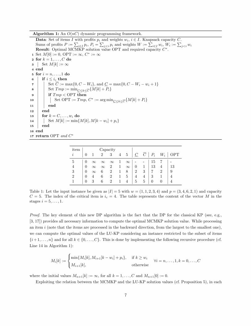
Algorithm 1: An O(nC) dynamic programming framework.

Data: Set of items I with profits pi and weights wi, i ∈ I. Knapsack capacity C.Sums of profits P :=

∑i∈I pi, Pi =

∑j<i pi and weights W :=

∑i∈I wi, Wi :=

∑j<i wi

Result: Optimal MCMKP solution value OPT and required capacity C∗.1 Set M [0] := 0, OPT :=∞, C∗ :=∞2 for k = 1, . . . , C do3 Set M [k] :=∞4 end5 for i = n, . . . , 1 do6 if i ≤ ic then7 Set C := max{0, C −Wi}, and C = max{0, C −Wi − wi + 1}8 Set Tmp := minC≤k≤C{M [k] + Pi}9 if Tmp < OPT then

10 Set OPT := Tmp, C∗ := arg minC≤k≤C{M [k] + Pi}11 end

12 end13 for k = C, . . . , wi do14 Set M [k] := min{M [k],M [k − wi] + pi}15 end

16 end17 return OPT and C∗

item Capacityi 0 1 2 3 4 5 C C Pi Wi OPT

5 0 ∞ ∞ ∞ 1 ∞ - - 15 7 -4 0 ∞ ∞ 2 1 ∞ 0 1 13 4 133 0 ∞ 6 2 1 8 2 3 7 2 92 0 4 6 2 1 5 4 4 3 1 41 0 3 6 2 1 4 5 5 0 0 4

Table 1: Let the input instance be given as |I| = 5 with w = (1, 1, 2, 3, 4) and p = (3, 4, 6, 2, 1) and capacityC = 5. The index of the critical item is ic = 4. The table represents the content of the vector M in thestages i = 5, . . . , 1.

Proof. The key element of this new DP algorithm is the fact that the DP for the classical KP (see, e.g.,

[3, 17]) provides all necessary information to compute the optimal MCMKP solution value. While processing

an item i (note that the items are processed in the backward direction, from the largest to the smallest one),

we can compute the optimal values of the LU-KP considering an instance restricted to the subset of items

{i+ 1, . . . , n} and for all k ∈ {0, . . . , C}. This is done by implementing the following recursive procedure (cf.

Line 14 in Algorithm 1):

Mi[k] :=

min{Mi[k],Mi+1[k − wi] + pi}, if k ≥ wiMi+1[k], otherwise

∀i = n, . . . , 1, k = 0, . . . , C

where the initial values Mn+1[k] :=∞, for all k = 1, . . . , C and Mn+1[0] := 0.

Exploiting the relation between the MCMKP and the LU-KP solution values (cf. Proposition 5), in each

7

iteration i (starting from an item i such that i ≤ ic) we then obtain the optimal MCMKP solution value,

assuming all unprocessed items (i.e., those from the set {1, . . . , i− 1}) are taken in the solution. The value

of this solution is stored in the variable Tmp (cf. Line 8), and the globally optimal solution is updated

correspondingly. Observe that the items {1, . . . , i − 1} determine the remaining capacity of the knapsack

(which is given as C) that has to be filled using items from {i + 1, . . . , n}, whereas C is determined by to

the fact that the packing has to be maximal and that the item i is the smallest one taken out of the solution

(cf. Property 2). This concludes the proof.

Observe that, so far, the Algorithm 1 only returns the optimal solution value OPT and the required

knapsack capacity C∗. In order to recover the optimal solution S∗, there exist two possibilities. At the

cost of increasing the space complexity from O(n + C) to O(nC), the optimal solution can be recovered in

O(n) time. To this end, it is sufficient to store the information whether the item i was added to the LU-KP

knapsack in the current iteration or not, for each weight k ∈ {0, . . . , C} and in each iteration i = n, . . . , 1.

We keep track of the pointers Ai[k] ∈ {0, 1} with the following meaning:

Ai[k] :=

1, if Mi[k] = Mi+1[k − wi] + pi

0, otherwise (i.e, if Mi[k] = Mi+1[k]), ∀i = n, . . . , 1, k = 0, . . . , C

After obtaining the optimal solution value OPT and the required capacity C∗, we can compute the optimal

MCMKP solution S∗ by applying a slight modification of the back-tracking procedure for the standard KP

(for further details concerning this back-tracking see, e.g. Section 2.3 in [14]). In the following, we explain

necessary modifications to this procedure. If A1[C∗] = 1, starting from the cell A1[C∗], the back-tracking

procedure is applied directly. If, otherwise, A1[C∗] = 0, we first initialize S∗ = {1, . . . , i∗ − 1}, where i∗ is

the smallest index such that Ai∗ [C∗] = 1. Starting from Ai∗ [C

∗], we then continue enlarging S∗ following

the standard back-tracking procedure.

In the following we show that the optimal solution can be recovered, while keeping the space complexity

O(n+ C).

Proposition 6. The optimal solution and the optimal solution value of the MCMKP can be computed in

O(nC) time and O(n+ C) space.

Proof. We refer to the recursive procedure for recovering the optimal solution of the classical KP described

in Section 3.3 of [14]. This procedure runs in O(nC) time and requires the four properties listed below to be

satisfied by our problem. Let in the following OPT(I, k) denote the optimal MCMKP value for the instance

(I, p, w, k) for any k = 0, . . . , C, and let S∗(I, k) be the corresponding optimal solution. The properties are

as follows:

1. There exists a procedure Solve(I, C) which computes for every integer k = 0, . . . , C the value OPT(I,

k) and requires O(nC) time and O(n+ C) space.

2. If n = 1, then Solve(I, C) also computes the optimal solution S∗(I, k) for all k = 0, . . . , C.

3. For every partitioning I1, I2 of I, there exist capacities C1, C2 such that C1 + C2 = C and OPT(I1,

C1) ∪OPT(I2, C2) = OPT(I, C), and

8

4. For every partitioning I1, I2 of I with |I2| = 1, and arbitrary capacities C1, C2, there exists a procedure

Merge that combines OPT(I1, C1) and OPT(I2, C2) into OPT(I1 ∪ I2, C1 + C2) in O(C1) time.

Regarding the first property, observe that a minor modification of the proposed Algorithm 1 is required, in

which we keep track of the optimal MCMKP solution value for all k = 0, . . . , C, and not only for k = C.

More precisely, for each k = 0, . . . , C, one has to keep track of C, C and OPT, which means that the space

complexity increases from C + n to 4C + n.

The remaining properties are trivially satisfied. Hence, by recursively calling the Solve procedure over

an arbitrary chosen non-trivial partitioning (I1, I2) of I, one can rebuild the optimal solution S∗(I, C) in

O(nC) time.

4. MIP Models for the MCMKP

Several MIP and constraint programming (CP) formulations for the MCMKP have been proposed in [7]

where it has been demonstrated that CP formulations are not competitive against MIP models. In the

following, we first recapitulate the two best performing MIP formulations among them, and then we derive

new theoretical results concerning the strength of their LP-relaxations. The results are derived using the

LP-duality theory and the theory of Benders decomposition.

4.1 An ILP Formulation for the MCMKP in the Natural Variable Space

In the following let the binary variables xi be set to one if the item i is selected, and to zero, otherwise. Each

feasible solution has to fit into the knapsack, but it also has to ensure the maximal packing property (i.e.,

adding an arbitrary additional item left outside of the solution, results in exceeding the knapsack capacity).

The formulation given below exploits the Proposition 1, and considers only the items left outside of S whose

weight does not exceed the critical weight. Let Cc = C − wc. The model reads as follows:

(F) min∑i∈I

pixi (4)∑i∈I

wixi ≤ C (5)∑j∈I,j 6=i

wjxj + wi(1− xi) ≥ (C + 1)(1− xi) ∀i ∈ I : i ≤ ic (6)

∑j∈I

wjxj ≥ Cc + 1 (7)

xi ∈ {0, 1} ∀i ∈ I (8)

Constraint (5) is a knapsack constraint stating that the weight of all selected items cannot exceed the available

capacity C. Inequalities (6) are based on Proposition 1 and Property 2 – they make sure that adding each

additional item i such that i ≤ ic will exceed the total capacity. We will refer to them as covering inequalities

associated to items i ≤ ic. Finally, the global covering constraint is derived from the global lower bound

9

given in Proposition 1. The constraint is redundant in the ILP formulation, but it improves the quality of

LP-bounds (see [7]).

Furthermore, coefficients of the covering constraints (6) and (7) can be down-lifted as shown in the

following Proposition.

Proposition 7 ([7]). For any i ∈ I, i ≤ ic, the associated covering inequalities (6) can be down-lifted to:∑j∈I,j 6=i

min{wj , Ci + 1}xj + min{wc, Ci + 1}xi ≥ Ci + 1 (9)

Similarly, coefficients of the constraint (7) can be down-lifted to min{wj , Cc + 1}, for all j ∈ I.

Observe that after this lifting, the covering inequality (6) associated to ic and the global covering in-

equality (7) become identical. In the following, we will denote by (Fl) the lifted formulation (F), in which

constraints (6) and (7) are replaced by their lifted counterparts as described in Proposition 7.

4.2 An Extended Formulation

Recall that for any knapsack solution to be feasible for the MCMKP it is sufficient that adding the weight

of the smallest item left out of the knapsack already violates the capacity C. Our next model encodes this

information by extending the previous model with a single non-negative continuous variable z modeling the

weight of a smallest item that is left out of the solution. The model reads as follows:

(Fe) min∑i∈I

pixi∑i∈I

wixi ≤ C (10)∑i∈I

wixi + z ≥ C + 1 (11)

z ≤ wc − (wc − wi)(1− xi) ∀i ∈ I, i ≤ ic (12)

xi ∈ {0, 1} ∀i ∈ I (13)

z ≥ 0 (14)

Validity of this model can be easily verified. Coupling constraints (12) make sure that z ≥ 0 is at most

the weight of the smallest item not included in the solution. Due to the covering constraint (11) and the

minimization objective function (with pi ≥ 0), it follows that z will be exactly the weight of the smallest item

left outside. For the same reasons as above (cf. Proposition 1), it is not necessary to impose constraints (12)

for i > ic.

Compared to the model (F) from above, this model contains only a single additional variable, but, thanks

to the reformulation, the structure of the constraint matrix is significantly simplified. Besides the packing

constraint (10) and the covering constraint (11), the remaining matrix has a diagonal structure, plus one

column of ones (corresponding to the variable z). Therefore, it is expected that the general-purpose MIP

solvers can be even more efficient when solving (Fe) than the formulation (F).

10

We now derive an interesting connection between (Fe) and (F). It turns out that by applying the Benders

decomposition to (Fe) and projecting out the z variable, we end up with two very similar models.

Proposition 8. Projecting out z variables from (Fe) results in the formulation (F) in which constraints (6)

are down-lifted as follows: ∑j∈I,j 6=i

wjxj + wcxi ≥ Ci + 1

Proof. After eliminating all constraints involving z variable from the (Fe), the reduced master problem boils

down to the classical KP, but with the minimization objective:

min{pTx | wTx ≤ C, x is binary } (15)

A solution x of the master problem (15) is feasible if and only if we can find z that satisfies the following

constraints:

z ≥ C + 1−∑j∈I

wj xj (γ) (16)

−z ≥ −wi − (wc − wi)xi ∀i ∈ I : i ≤ ic (αi) (17)

z ≥ 0 (18)

Farkas lemma states that a linear system of inequalities {Az ≥ b, z ≥ 0} is feasible if and only if uT b ≤ 0

for all u ≥ 0 such that uTA ≤ 0. Let γ ≥ 0 be a dual variable associated to constraint (16) and let αi ≥ 0,

for all i ≤ ic be dual variables associated to (17). By Farkas lemma, x is feasible if and only if the optimal

solution value of the following system is non-positive:

max γ(C + 1−∑j∈I

wj xj) +∑i≤ic

αi(−wi − (wc − wi)xi) (19)

s.t. −∑i≤ic

αi + γ ≤ 0 (20)

α, γ ≥ 0 (21)

We observe that the optimal solution of the latter problem satisfies γ =∑i≤ic αi, since x is a feasible master

solution and hence it satisfies the knapsack capacity constraint, so we have C + 1−∑i wixi > 0. The dual

problem now boils down to:

maxα≥0

∑i≤ic

αi

C + 1−∑j∈I

wj xj − wi − (wc − wi)xi

This problem is unbounded (i.e., x is infeasible) if and only if there exists i ∈ I, i ≤ ic, such that

C + 1−∑

j∈I,j 6=i

wj xj − wcxi − wi > 0

Hence, all infeasible solutions x of the master problem can be cut-off by the following (compact) family of

11

feasibility constraints: ∑j∈I,j 6=i

wjxj + wcxi ≥ C + 1− wi, ∀i ∈ I : i ≤ ic,

what concludes the proof.

Corollary 1. The value of the LP-relaxation of (Fe) and of the following model are the same:

min∑i∈I

pixi∑i∈I

wixi ≤ C (22)∑j∈I,j 6=i

wjxj + wcxi ≥ Ci + 1 ∀i ≤ ic (23)

xi ∈ {0, 1} ∀i ∈ I

Corollary 2. If min{wj , Cc + 1} = wj, for all j ∈ I, then the LP-relaxation bounds of (Fl) and (Fe) are

the same.

Corollary 3. In general, LP-relaxation bounds of (Fl) can be stronger than those of (Fe).

In order to see that this is the case, consider the same example given in Table 1. Inequalities (9) and

(23) are identical for all i < ic, however for i = ic = 4, the inequality (9) in the model (Fl) is x1 +x2 + 2x3 +

3x4 + 3x5 ≥ 3, whereas the associated inequality (23) is weaker and reads x1 + x2 + 2x3 + 3x4 + 4x5 ≥ 3.

5. Equivalence Between MCMKP and MPMKC

In this section we prove the following result:

Proposition 9. Any feasible solution S of the MCMKP on an instance (I, p, w,C) corresponds to a feasible

solution S′ = I \ S of the MPMKC on instance (I, p, w,C ′) where C ′ = W − C.

Before showing this result, we will discuss the critical item of the MPMKC and a counterpart of the

extended formulation for the MPMKC. As above, we assume that items are sorted in non-decreasing order

according to their weights. Observe that the index of the critical item and the corresponding weight for the

MPMKC are calculated differently.

Definition 6 (MPMKC-Critical Weight and MPMKC-Critical Item). Denote by

ic = arg max{i ∈ I |∑j≥i

wj ≥ C}

the index of a MPMKC-critical item, i.e., the index of the first item that covers the knapsack, assuming all

i ≥ ic will be taken as well. The MPMKC-critical weight, denoted by wc, is the weight of the critical item,

i.e., wc = wic .

12

Proposition 10. The weight of the smallest item taken into any feasible MPMKC solution is bounded from

above by the critical weight wc, i.e.:

S is feasible ⇒ mini∈S

wi ≤ wc.

Consequently, the capacity used by any minimal knapsack cover is bounded from above as:

w(S) ≤ C + wc − 1.

Proof. Suppose S is a feasible MPMKC solution such that mini∈S wi > wc. Hence, S contains only items i

such that i > ic. However, by definition of the critical item, it follows that∑i:i>ic

wi ≤ C − 1 which means

that S is not a cover, a contradiction.

For the second part of the proposition, observe that capacity used by any feasible solution can be bounded

from above as C − 1 + wmax. However, knowing that removal of even the smallest item from this solution

results in capacity ≤ C − 1, leads to the conclusion that w(S) ≤ C − 1 + wc.

We can now prove the following lemma:

Lemma 1. We have that the index of a critical item ic for the MCMKP on instance (I, p, w,C) and the

index of a critical item ic for the MPMKC on instance (I, p, w,C ′) are the same, i.e., it holds:

arg min{i ∈ I |∑j≤i

wj > C} = arg max{i ∈ I |∑j≥i

wj ≥W − C}

Proof. Observe that∑j≤i wj can be written as W −

∑j>i wj so that ic is the smallest index of an item i

such that∑j>i wj < W − C. Hence, for ic it must hold:

∑j≥ic wj ≥ W − C. Obviously, for any i < ic,

we have∑j≥i wj ≥

∑j≥ic wj ≥ W − C. So, we conclude that ic is the maximal index of an item that

satisfies the latter property, which exactly corresponds to the definition of the index of a critical item ic for

the instance (I, p, w,C ′) for the MPMKC.

Extended Formulation for the MPMKC Let binary variables yi be set to one if item i is taken into

MPMKC solution, and to zero, otherwise. The following (extended) MIP formulation is a valid model for

the MPMKC, in which the variable z takes the weight of the minimum item in the solution.

max∑i∈I

piyi (24)∑i∈I

wiyi ≥ C (25)∑i∈I

wiyi − z ≤ C − 1 (26)

z ≤ wiyi + wc(1− yi) ∀i ∈ I : i ≤ ic (27)

y ∈ {0, 1} ∀i ∈ I (28)

z ≥ 0 (29)

13

Constraint (25) ensures that the solution is a knapsack cover, whereas constraint (26) makes sure that this

cover is minimal, i.e., whenever the smallest item is taken out of the solution, the weight of the remaining

selected items remains ≤ C − 1. Finally, constraints (27) ensure that z takes the value of the smallest item

in the solution, by exploiting the property of Proposition 10.

Proof of Proposition 9. The linear transformation yi = 1− xi, for all i ∈ I, allows to translate the extended

formulation (Fe) for the MCMKP into the extended formulation (24)-(29) for the MPMKC and vice versa.

We start with the model (Fe) given in Section 4.2, and apply this linear transformation. The model (Fe)

translates into the following one:

P + min∑i∈I

(−pi)yi∑i∈I

wiyi ≥ C ′ (30)∑j∈I

wjyj − z ≤ C ′ − 1 (31)

z ≤ wc − (wc − wi)yi ∀i ∈ I : i ≤ ic (32)

yi ∈ {0, 1} ∀i ∈ I

Observing that the minimization can be turned into maximization and, using the facts that C ′ = C −Wand ic = ic (see Lemma 1), it immediately follows that the transformed model and the model (24)-(29) are

the same for the instance (I, p, w,C ′), which concludes the proof.

Hence, in order to solve MPMKC on the instance (I, p, w,C), it is sufficient to solve the complementary

MCMKP on the instance (I, p, w,W −C) and take the items left out of the optimal MCMKP solution. The

above result together with Proposition 5 implies the following:

Corollary 4. The problem MPMKC on an instance (I, p, w,C) is weakly NP-hard and there exists a DP

algorithm that solves it in O(n(W − C)) time.

6. Computational Study

The primary goal of this computational study is to compare the performances of the Dynamic Programming

(DP) described in Section 3 with the MIP models discussed in Section 4. To the best of our knowledge, these

models are the best formulations proposed so far in literature. The computational results presented in [7]

allow us to conclude that both models, i.e., (Fl) and (Fe), outperform in terms of computational performance

the DP algorithm proposed in [7]. Recall that this latter DP algorithm runs in O(n2C) time. As a matter

of fact, it already struggles to tackle instances with 100 items and it is effective only in solving small size

instances (see [7] for more details). For this reason, we decided to exclude it from the this computational

study.

The experiments have been performed on a computer with a 2.5 Ghz Intel Xeon CPU processor and 64GB

RAM, running a 64 bits Linux operating system. All the codes were compiled with g++ (version 4.8.4) using

-O3 as optimization option. We have tested the MIP models using Cplex 12.6.3, single-threaded (called

14

for brevity Cplex in the following). All Cplex parameters are at their default values except the optimality

tolerances which have been set to 0 in order to be able to compare the solutions of the models with the

solutions of the DP algorithm. In all our tests we imposed a time limit of 1 000 seconds and memory limit

of 3GB.

A second goal of this computational study is also to determine the size of the instances which can be

solved to proven optimality within short running time. In [7], a very diverse banchmark set of instances

with up to 2 000 items has been proposed. In this manuscript we consider the same classes of instances, but,

in order determine the limits of the proposed exact methods, we also introduce larger instances with up to

5 000 items. In the following the test bed of instances is described in details.

6.1 Benchmark Instances

Nine classes of MCMKP instances have been randomly generated by defining weights and profits following

the procedure for the classical KP described in [15] (u.r. stands for “uniformly random integer”). The

instance generator is available at [20].

1. Uncorrelated: wj u.r. in [1, R], pj u.r. in [1, R].

2. Weakly correlated: wj u.r. in [1, R], pj u.r. in [wj −R/10, wj +R/10] so that pj ≥ 1.

3. Strongly correlated: wj u.r. in [1, R], pj = wj +R/10.

4. Inverse strongly correlated: pj u.r. in [1, R], wj = pj +R/10.

5. Almost strongly correlated: wj u.r. in [1, R], pj u.r. in [wj+R/10−R/500, wj+R/10+R/500].

6. Subset-sum: wj u.r. in [1, R], pj = wj .

7. Even-odd subset-sum: wj even value u.r. in [1, R], pj = wj , c odd.

8. Even-odd strongly correlated: wj even value u.r. in [1, R], pj = wj +R/10, c odd.

9. Uncorrelated with similar weights: wj u.r. in [100R, 100R+R/10], pj u.r. in [1, R].

For each instance class and value of R ∈ {1000, 10000}, we generated 30 MCMKP instances by considering

all combinations of (i) number of items n ∈ {10, 20, 30, 40, 50, 100, 500, 1000, 2000, 5000}; (ii) capacity C ∈{b25%W c, b50%W c, b75%W c} (and C increased by 1, if even, for classes 7 and 8); thus obtaining 540

MCMKP instances.

6.2 Initialization and Primal Heuristics

Thanks to extensive preliminary tests we observed that Cplex sometimes struggles to find good primal

solutions for models (Fl) and (Fe). Accordingly we decided to implement Initialization and Primal Heuristics.

The initialization heuristic is the greedy-comb proposed in [7]. The approach consists of two basic steps:

(i) examining the items according to a pre-specified order,

(ii) adding the current item to the solution iff its weight does not exceed the current residual capacity.

15

Six different orderings are incorporated in this greedy-comb procedure, and the best solution found is returned.

The procedure greedy-comb is very fast and produces high quality initial solutions, with gaps to the optimal

solutions being between 1% and 6% on our benchmark set (see [7] for further details).

In addition to this Initialization Heuristic, we apply a new and effective Primal Heuristic that can be

executed within the nodes of the branch-and-cut scheme of Cplex. Once a LP-solution x is calculated, we

call greedy-comb by weighting the item scores using the values of xi, for all i ∈ I. Then the items are resorted

according to the new score values, and greedy-comb is then executed. This primal heuristic produces effective

speedups as it is shown in the next Sections.

6.3 Quality of the LP Relaxation of the Models

Table 2 shows the gaps between the optimal solution value and the value of the Linear Programming (LP)

relaxations of (Fl) and (Fe). The table is structured according to the instance categories, i.e., each entry

reports the average gap of the 60 instances of the considered category. The gaps are calculated as (z∗ −zR)/z∗100, where z∗ is the optimal solution value and zR is the optimal value of the LP relaxation. We

observe that the gaps of both formulations are very similar, for categories 1, 2, 4, 5 and 9 the average gaps

coincide. The instance of category 1 are characterized by the largest average gaps (12.30%). Aside from this

category and category 9 with an average gap of 5.98%, the gaps for all other categories are under 3%.

Table 2: Average percentage LP gaps for (Fl) and (Fe) .

instance category1 2 3 4 5 6 7 8 9

(Fl) 12.30 2.87 2.47 2.27 2.41 2.63 2.64 2.56 5.98(Fe) 12.30 2.87 2.51 2.27 2.41 2.65 2.66 2.59 5.98

6.4 Comparison Between the Proposed Exact Methods

The performances of the DP algorithm, the (Fl) and the (Fe) are compared. For the two MIP models

additional configurations are considered, in which the basic models are enhanced by our Initial and Primal

Heuristics (denoted by (Fl)H and (Fe)

H). Instances not solved to proven optimality within the timelimit

of 1 000 seconds, or which have terminated due to the memorylimit, are counted as 1 000 seconds in the

following results.

In order to give a graphical representation of the relative performance of the proposed approaches, we

report a performance profile in Figure 1. For each instance we compute a normalized time τ as the ratio

of the computing time of the considered solution method over the minimum computing time for solving the

instance to optimality. For each value of τ in the horizontal axis, the vertical axis reports the percentage of

the instances for which the corresponding method spent at most τ times the computing time of the fastest

method. It shows that DP outperforms the MIP models both in terms of speed and number of solved

instances. In about 85% of the instances the DP algorithm is the fastest one and it is capable to solve almost

99% of the instances to proven optimality. The second best approach is (Fe)H followed by (Fe). The models

(Fl)H and (Fl) have similar poor performances with respect to the DP algorithm. In the following, we will

take a more detailed look at the results.

16

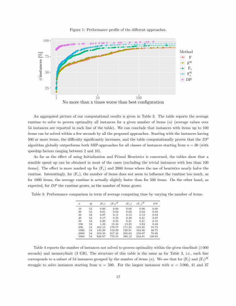
Figure 1: Performance profile of the different approaches.

●●●●

●●

●●

●●●●●●●●●●●●●●●●●●●●●●●●●●●●●●●●●●●●●●●●●●●●●●●●●●●●

●●●●●●●●●●●●●●●●●●●●●●●●●●●●●●

●●●●●●●●●●●●●●●●●●●●●

●● ●●●●●●●●●●●●●●●●●●●●●●●

●●●●●●●●● ●●●● ●●●●●●●●

●● ●●●●●●●●●●●●●●●●●●●●●●●●●●●●●

●●●●●●●● ●●●●●●●●●●●●● ●●●●●●●● ●●●●●● ● ● ● ●● ● ● ● ●

25

50

75

100

1 10 100No more than x times worse than best configuration

#in

stan

ces

[%] Method

● F

FH

Fe

FeH

DP

An aggregated picture of our computational results is given in Table 3. The table reports the average

runtime to solve to proven optimality all instances for a given number of items (n) (average values over

54 instances are reported in each line of the table). We can conclude that instances with items up to 100

items can be solved within a few seconds by all the proposed approaches. Starting with the instances having

500 or more items, the difficulty significantly increases, and the table computationally proves that the DP

algorithm globally outperforms both MIP-approaches for all classes of instances starting from n = 30 (with

speedup factors ranging between 2 and 10).

As far as the effect of using Initialization and Primal Heuristics is concerned, the tables show that a

sensible speed up can be obtained in most of the cases (excluding the trivial instances with less than 100

items). The effect is more marked up for (Fe) and 2000 items where the use of heuristics nearly halve the

runtime. Interestingly, for (Fe), the number of items does not seem to influence the runtime too much, as

for 1000 items, the average runtime is actually slightly faster than for 500 items. On the other hand, as

expected, for DP the runtime grows, as the number of items grows.

Table 3: Performance comparison in term of average computing time by varying the number of items.

n # (Fl) (Fl)H (Fe) (Fe)H DP

10 54 0.00 0.00 0.00 0.00 0.0020 54 0.01 0.02 0.02 0.02 0.0230 54 0.07 0.11 0.12 0.13 0.0440 54 0.17 0.35 0.39 0.41 0.0750 54 0.20 0.35 0.21 0.21 0.10100 54 1.22 13.16 13.23 5.83 0.42500 54 164.15 178.57 171.25 145.85 10.721000 54 145.29 152.99 128.81 104.30 48.752000 54 333.35 317.16 292.83 159.67 76.865000 54 828.87 770.35 389.12 244.81 149.93

Table 4 reports the number of instances not solved to proven optimality within the given timelimit (1 000

seconds) and memorylimit (3 GB). The structure of this table is the same as for Table 3, i.e., each line

corresponds to a subset of 54 instances grouped by the number of items (n). We see that for (Fl) and (Fl)H

struggle to solve instances starting from n = 500. For the largest instances with n = 5 000, 41 and 37

17

instances remain unsolved by (Fl) and (Fl)H , respectively. Also (Fe) and (Fe)

H struggle to solve instances

starting from n = 500 but more instances could be solved, i.e, only 17 and 10 instances remain unsolved

by (Fe) and (Fe)H , respectively. A possible explanation is the density of the model (Fl), that causes the

memorylimit to be reached more often that for the model (Fl) (which possesses an almost diagonal structure

of the constraint matrix). We therefore conclude that model (Fe) outperforms model (Fl) in terms of the

number of instances solved to proven optimality. Table 4 also demonstrates the beneficial effect of our

heuristic algorithms: globally, (Fl)H solves 4 more instance than (Fl) and (Fe)

H solves 14 more instances

than (Fe).

As far as the performances of the DP are concerned, the DP algorithm only starts struggling to solve

instances from n = 1 000 and only 10 out of 540 instances remains unsolved by this exact approach. As a

comparison, model (Fl)H fails in total in 58 instances while model (Fl)

H fails in 27 instances. This allows

us to conclude that our new DP algorithm computationally outperforms both models (Fl)H and (Fe)

H also

for the total number of instances solved to proven optimality.

Table 4: Instances unsolved within timelimit and memorylimit varying the number of items.

n # (Fl) (Fl)H (Fe) (Fe)H DP

10 54 0 0 0 0 020 54 0 0 0 0 030 54 0 0 0 0 040 54 0 0 0 0 050 54 0 0 0 0 0100 54 0 0 0 0 0500 54 8 9 9 7 01000 54 5 5 6 5 22000 54 8 7 9 5 35000 54 41 37 17 10 5

It is worth mentioning that all instances which remain unsolved for DP are of category 9, which has

much larger weights compared to the other instance classes. This class of instances is specifically conceived

to create instances which are hard for DP algorithms. In order to have a clear picture on the performances

of the proposed exact methods on the different class of instances we report Table 5. Instances terminated

due to memorylimit are counted as taking 1 000 seconds as for the other tables. The table shows the average

runtime to solve to proven optimality the instances grouped by category. Each column reports averages

values for 60 instances and on the rows the different exact methods are given.

Table 5: Performance comparison in term of average computing time grouping istances by category.

instance category1 2 3 4 5 6 7 8 9

# 60 60 60 60 60 60 60 60 60

(Fl) 115.47 97.85 113.94 287.77 213.64 164.23 149.37 98.06 86.94

(Fl)H 119.10 80.40 99.42 293.30 211.08 157.00 166.98 73.05 90.56

(Fe) 17.25 11.14 223.68 270.88 111.09 56.06 23.10 154.65 28.53

(Fe)H 17.82 8.73 92.56 240.61 99.01 45.54 13.52 46.49 30.82DP 5.72 5.85 5.49 6.89 5.45 5.34 5.44 5.47 212.57

For both MIP-approaches (regardless of using the heuristics or not), instance category 4 is the most

difficult one, while at least for (Fe) (and (Fe)H), instances of categories 1 and 2 are rather easy. For all

categories except category 9, the DP algorithm clearly outperforms the MIP-approaches. As previously

18

mentioned, the instances of category 9 have much larger coefficients which leads to a higher value of C and

accordingly the performances of the DP algorithm deteriorates. For the instances of category 9, (Fe) tends

to be the best approach. Finally, we can conclude that (Fe) outperforms (Fl) for all categories of instances.

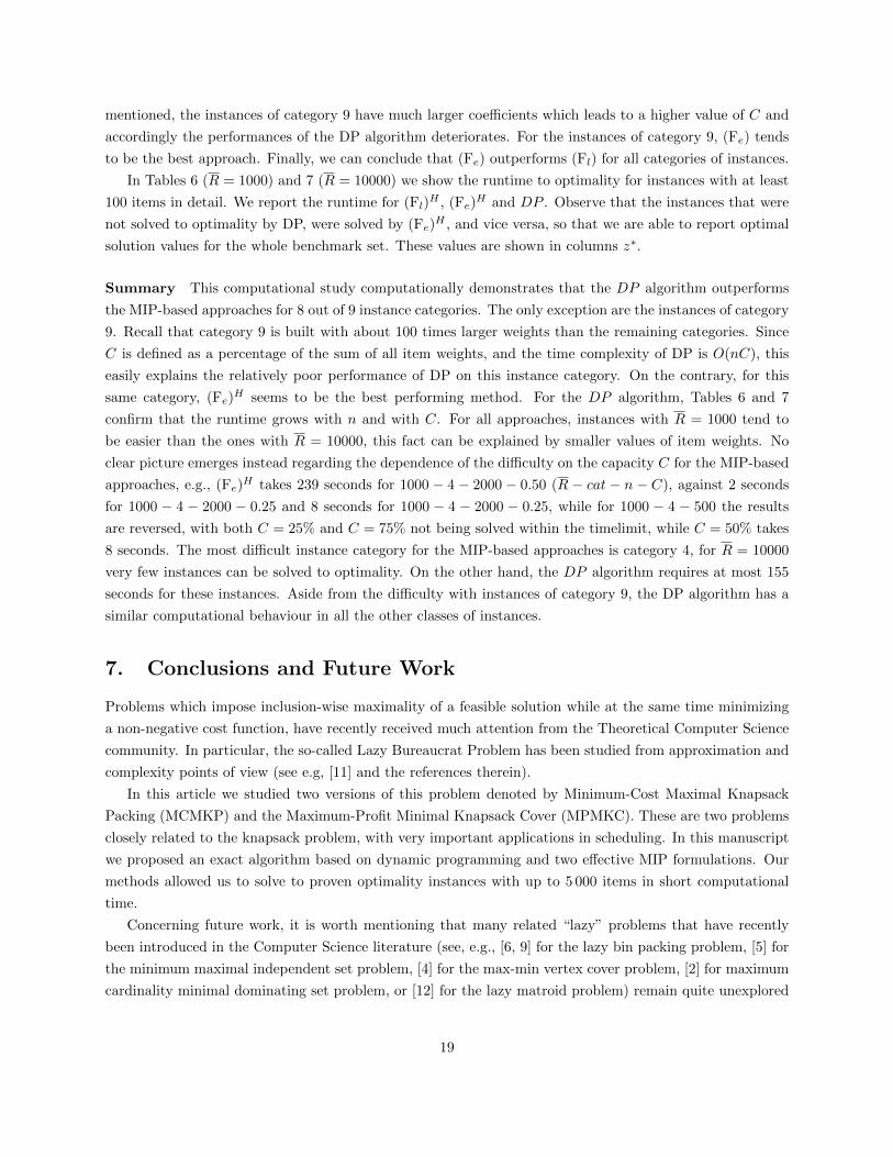
In Tables 6 (R = 1000) and 7 (R = 10000) we show the runtime to optimality for instances with at least

100 items in detail. We report the runtime for (Fl)H , (Fe)

H and DP . Observe that the instances that were

not solved to optimality by DP, were solved by (Fe)H , and vice versa, so that we are able to report optimal

solution values for the whole benchmark set. These values are shown in columns z∗.

Summary This computational study computationally demonstrates that the DP algorithm outperforms

the MIP-based approaches for 8 out of 9 instance categories. The only exception are the instances of category

9. Recall that category 9 is built with about 100 times larger weights than the remaining categories. Since

C is defined as a percentage of the sum of all item weights, and the time complexity of DP is O(nC), this

easily explains the relatively poor performance of DP on this instance category. On the contrary, for this

same category, (Fe)H seems to be the best performing method. For the DP algorithm, Tables 6 and 7

confirm that the runtime grows with n and with C. For all approaches, instances with R = 1000 tend to

be easier than the ones with R = 10000, this fact can be explained by smaller values of item weights. No

clear picture emerges instead regarding the dependence of the difficulty on the capacity C for the MIP-based

approaches, e.g., (Fe)H takes 239 seconds for 1000 − 4 − 2000 − 0.50 (R − cat − n − C), against 2 seconds

for 1000 − 4 − 2000 − 0.25 and 8 seconds for 1000 − 4 − 2000 − 0.25, while for 1000 − 4 − 500 the results

are reversed, with both C = 25% and C = 75% not being solved within the timelimit, while C = 50% takes

8 seconds. The most difficult instance category for the MIP-based approaches is category 4, for R = 10000

very few instances can be solved to optimality. On the other hand, the DP algorithm requires at most 155

seconds for these instances. Aside from the difficulty with instances of category 9, the DP algorithm has a

similar computational behaviour in all the other classes of instances.

7. Conclusions and Future Work

Problems which impose inclusion-wise maximality of a feasible solution while at the same time minimizing

a non-negative cost function, have recently received much attention from the Theoretical Computer Science

community. In particular, the so-called Lazy Bureaucrat Problem has been studied from approximation and

complexity points of view (see e.g, [11] and the references therein).

In this article we studied two versions of this problem denoted by Minimum-Cost Maximal Knapsack

Packing (MCMKP) and the Maximum-Profit Minimal Knapsack Cover (MPMKC). These are two problems

closely related to the knapsack problem, with very important applications in scheduling. In this manuscript

we proposed an exact algorithm based on dynamic programming and two effective MIP formulations. Our

methods allowed us to solve to proven optimality instances with up to 5 000 items in short computational

time.

Concerning future work, it is worth mentioning that many related “lazy” problems that have recently

been introduced in the Computer Science literature (see, e.g., [6, 9] for the lazy bin packing problem, [5] for

the minimum maximal independent set problem, [4] for the max-min vertex cover problem, [2] for maximum

cardinality minimal dominating set problem, or [12] for the lazy matroid problem) remain quite unexplored

19

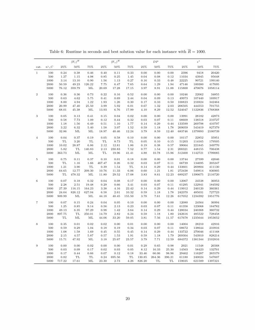
Table 6: Runtime in seconds and best solution value for each instance with R = 1000.

(Fl)H (Fe)H DP z∗

cat. n�C 25% 50% 75% 25% 50% 75% 25% 50% 75% 25% 50% 75%

1 100 0.24 0.38 0.46 0.40 0.11 0.33 0.00 0.00 0.00 2396 9418 20420

500 1.27 1.15 4.98 0.85 0.25 1.45 0.04 0.08 0.12 11034 43945 95648

1000 3.14 13.10 0.90 1.56 1.13 0.27 0.16 0.33 0.48 22225 90721 199140

2000 50.59 49.23 126.22 7.75 6.47 7.65 0.64 1.29 1.94 47146 189380 417695

5000 76.12 359.79 ML 20.69 17.28 17.15 3.97 8.91 11.88 115800 470676 1058114

2 100 0.36 0.36 0.73 0.22 0.16 0.52 0.00 0.00 0.00 10246 22062 34855

500 0.63 4.62 5.75 0.41 0.69 2.44 0.04 0.09 0.13 49973 107440 169917

1000 8.00 4.94 1.22 1.93 1.26 0.30 0.17 0.33 0.50 100823 216924 342464

2000 20.99 47.40 25.50 3.99 5.92 6.01 0.67 1.32 2.03 206505 444553 701755

5000 68.01 45.38 ML 13.93 6.76 17.99 4.10 8.29 12.52 524047 1122836 1768368

3 100 0.05 0.13 0.41 0.15 0.04 0.02 0.00 0.00 0.00 13991 28182 42873

500 0.58 7.73 1.09 0.12 0.44 0.32 0.03 0.07 0.11 68609 138518 210727

1000 1.18 1.56 6.49 0.51 1.10 1.77 0.14 0.29 0.44 133599 269798 410797

2000 3.22 6.32 5.40 1.58 3.07 1.52 0.59 1.18 1.78 269059 543419 827379

5000 32.86 ML ML 18.97 40.46 12.24 3.79 8.59 12.40 683746 1379993 2100739

4 100 0.04 0.37 0.19 0.05 0.58 0.10 0.00 0.00 0.00 10117 22852 35951

500 TL 3.20 TL TL 8.73 TL 0.05 0.10 0.15 51203 114165 179505

1000 10.02 28.87 6.86 2.12 12.81 1.86 0.19 0.38 0.57 99064 221845 349770

2000 5.82 TL 140.83 2.13 230.83 7.52 0.77 1.54 2.31 200321 448155 706438

5000 363.73 ML ML TL 19.96 41.41 4.88 10.78 15.96 512400 1142721 1799085

5 100 0.75 0.11 0.37 0.10 0.01 0.18 0.00 0.00 0.00 13744 27599 42046

500 TL 1.16 1.66 467.47 0.26 0.32 0.03 0.07 0.11 66739 134695 205247

1000 1.21 3.90 TL 0.39 1.54 TL 0.14 0.29 0.44 133601 269804 411130

2000 64.65 12.77 209.30 10.76 11.33 6.06 0.60 1.21 1.81 272438 549814 836905

5000 TL 478.32 ML 11.80 29.52 17.08 3.83 8.61 12.23 689237 1390675 2116720

6 100 0.07 0.18 0.32 0.04 0.08 0.17 0.00 0.00 0.00 12067 24538 36953

500 2.28 2.51 19.48 0.29 0.66 3.41 0.03 0.07 0.11 61295 122941 184592

1000 27.39 116.15 164.23 3.38 4.16 22.42 0.14 0.29 0.44 119912 240120 360361

2000 24.64 826.12 627.04 6.58 2.61 10.32 0.59 1.18 1.78 242370 485031 727723

5000 909.99 ML ML 44.18 40.45 155.50 3.78 7.61 12.26 617052 1234392 1851776

7 100 0.07 0.15 0.24 0.04 0.05 0.10 0.00 0.00 0.00 12080 24564 36994

500 1.25 0.85 9.14 0.56 2.13 0.23 0.03 0.07 0.11 61358 123068 184782

1000 49.13 6.35 97.29 0.98 1.42 3.64 0.14 0.29 0.44 120034 240368 360732

2000 897.75 TL 250.01 14.79 2.82 6.24 0.59 1.18 1.80 242616 485522 728458

5000 TL ML ML 44.06 33.20 59.05 3.81 7.56 11.57 617678 1235644 1853652

8 100 0.35 0.01 0.02 0.02 0.00 0.01 0.00 0.00 0.00 14004 28210 42916

500 0.59 0.29 1.04 0.18 0.19 0.34 0.03 0.07 0.11 68672 138644 210916

1000 1.08 1.58 1.69 0.45 0.55 0.45 0.14 0.29 0.44 133722 270046 411168

2000 2.15 4.57 5.87 0.57 1.53 1.91 0.59 1.18 1.79 269304 543910 828214

5000 15.71 47.92 ML 3.18 25.67 23.57 3.79 7.71 12.59 684372 1381344 2102816

9 100 0.00 0.00 0.02 0.00 0.00 0.01 0.29 0.65 0.98 2921 11548 26568

500 0.03 0.09 0.17 0.02 0.03 0.05 8.12 16.33 25.30 14563 58423 132701

1000 0.17 0.44 0.66 0.07 0.12 0.18 33.46 66.06 98.96 29462 116287 265579

2000 0.82 TL TL 0.24 695.56 TL 130.85 264.36 396.21 61180 240024 547607

5000 717.22 17.61 ML 23.30 2.73 4.26 826.20 TL TL 159035 621589 1397221

20

Table 7: Runtime in seconds and best solution value for each instance with R = 10000.

(Fl)H (Fe)H DP z∗

cat. n�C 25% 50% 75% 25% 50% 75% 25% 50% 75% 25% 50% 75%

1 100 3.19 20.29 4.68 1.35 20.22 2.13 0.02 0.04 0.06 21811 80166 179311

500 53.62 33.51 209.00 4.86 12.02 57.95 0.46 0.89 1.32 114523 459156 1039992

1000 43.44 834.24 49.45 21.51 181.38 10.50 1.71 3.38 5.16 224150 941497 2117198

2000 330.56 807.16 423.48 60.51 178.36 64.81 6.95 13.34 21.25 483979 1925732 4295218

5000 628.31 ML ML 120.47 64.96 176.26 44.68 86.53 127.29 1179665 4686830 10507765

2 100 0.10 0.13 0.32 0.08 0.07 0.24 0.02 0.05 0.07 85229 185013 292897

500 3.10 8.25 2.47 0.97 4.56 5.31 0.49 0.94 1.37 498746 1073343 1698472

1000 10.71 57.56 33.52 3.55 7.58 19.88 1.81 3.72 5.56 1028577 2201879 3468177

2000 145.06 144.01 685.58 18.73 36.83 90.64 7.15 14.44 21.59 2071531 4430501 6976442

5000 492.25 ML ML 24.54 134.98 112.60 44.24 89.06 130.24 5263091 11251628 17711417

3 100 0.17 53.55 296.85 0.33 80.08 34.27 0.01 0.02 0.04 118252 238588 363929

500 2.80 36.61 2.67 0.73 237.60 4.20 0.36 0.71 1.13 649309 1310618 2000927

1000 67.69 294.28 6.28 116.11 8.90 4.05 1.49 3.20 4.59 1351149 2726298 4156447

2000 92.90 13.36 10.70 975.22 TL 3.46 6.13 13.42 19.62 2747609 5545219 8442829

5000 ML ML ML TL TL TL 40.73 82.14 126.33 6926796 13981593 21278389

4 100 0.12 6.73 20.12 0.08 5.43 12.39 0.03 0.05 0.08 79817 186007 297960

500 TL TL TL TL TL TL 0.51 1.04 1.57 476256 1068850 1693224

1000 TL TL TL TL TL TL 1.96 4.10 6.36 1010792 2247788 3541015

2000 TL TL TL TL 89.59 TL 7.83 16.77 24.67 2066109 4591558 7222366

5000 ML ML ML TL TL TL 51.66 104.00 155.23 5230252 11605856 18236923

5 100 0.17 5.31 1.80 138.17 2.47 1.79 0.01 0.03 0.05 114770 230670 352572

500 TL TL TL TL TL 9.43 0.38 0.77 1.18 664526 1343087 2046816

1000 47.03 TL 7.19 40.64 TL 4.01 1.53 3.05 4.75 1349293 2725604 4150205

2000 343.94 220.77 247.50 95.10 28.10 7.73 6.53 13.19 19.48 2733192 5519666 8401427

5000 TL ML ML 24.60 TL 17.32 40.33 82.60 124.00 6909253 13944843 21218933

6 100 0.08 0.26 0.04 0.06 0.14 0.05 0.01 0.02 0.04 101130 204809 308231

500 4.78 32.60 36.67 1.13 3.75 12.74 0.36 0.72 1.08 580840 1163941 1747413

1000 37.97 125.58 169.78 4.18 7.62 48.17 1.49 3.03 4.49 1213512 2429569 3645954

2000 302.56 439.40 539.30 15.96 14.52 14.71 6.06 12.65 19.84 2474759 4952346 7430298

5000 ML ML ML 909.91 404.44 TL 40.36 80.72 121.34 6248810 12500605 18752821

7 100 0.08 0.27 0.05 0.06 0.12 0.05 0.01 0.02 0.04 101156 204848 308280

500 4.31 10.81 28.58 0.74 3.10 10.70 0.35 0.71 1.07 580892 1164068 1747602

1000 42.64 200.22 115.74 3.85 13.58 35.39 1.49 3.16 4.88 1213636 2429818 3646326

2000 168.13 279.62 845.65 13.94 90.86 43.43 6.64 12.56 19.33 2475004 4952838 7431034

5000 ML ML ML 14.07 223.02 188.44 41.21 83.21 124.01 6249436 12501856 18754698

8 100 0.16 0.53 289.00 0.62 0.24 10.76 0.01 0.02 0.04 118262 237710 363974

500 0.95 16.79 82.33 0.29 8.52 4.98 0.35 0.71 1.07 649372 1310744 2001116

1000 39.14 280.84 226.95 1.52 5.70 24.75 1.49 2.98 4.59 1351272 2726546 4156818

2000 5.90 288.46 28.49 5.09 TL 645.67 6.13 13.07 20.14 2747854 5545710 8443564

5000 ML 25.03 ML TL 5.87 7.71 40.53 87.43 120.95 6927422 13982844 21280266

9 100 0.00 0.00 0.01 0.00 0.00 0.01 3.31 6.73 10.06 18762 84731 207429

500 0.05 0.11 1.12 0.02 0.04 0.67 83.89 176.32 247.69 145911 596495 1326550

1000 8.79 4.10 0.84 0.56 2.03 0.23 346.45 TL TL 302563 1216230 2428114

2000 350.56 2.31 3.78 71.66 0.57 0.87 TL TL TL 628397 2428114 2428114

5000 306.25 14.59 ML 36.89 3.18 6.06 TL TL TL 1577597 2428114 2428114

21

from an exact point of view. With this article we hope to stimulate the research on this new and challenging

family of problems which can give rise to new solution properties and exact methods. Finally, it could be

interesting to study other variants of the classical knapsack problem in this “lazy” setting, such as quadratic

knapsack and covering problems [10, 19] or the multiple-choice knapsack problem [18].

Acknowledgments

The research of M. Sinnl was supported by the Austrian Research Fund (FWF, Project P 26755-N19).

References

[1] E. M. Arkin, M. A. Bender, J. S. Mitchell, and S. S. Skiena. The lazy bureaucrat scheduling problem.

Information and Computation, 184(1):129–146, 2003.

[2] C. Bazgan, L. Brankovic, K. Casel, H. Fernau, K. Jansen, K.-M. Klein, M. Lampis, M. Liedloff, J. Mon-

not, and V. T. Paschos. Upper domination: Complexity and approximation. In V. Mkinen, S. J. Puglisi,

and L. Salmela, editors, International Workshop on Combinatorial Algorithms, volume 9843 of Lecture

Notes in Computer Science, pages 241–252. Springer, 2016.

[3] R. Bellman. Dynamic Programming. Princeton University Press, 1957.

[4] N. Boria, F. Della Croce, and V. T. Paschos. On the max min vertex cover problem. Discrete Applied

Mathematics, 196:62–71, 2015.

[5] N. Bourgeois, F. Della Croce, B. Escoffier, and V. T. Paschos. Fast algorithms for min independent

dominating set. Discrete Applied Mathematics, 161(4):558–572, 2013.

[6] J. Boyar, L. Epstein, L. M. Favrholdt, J. S. Kohrt, K. S. Larsen, M. M. Pedersen, and S. Whlk. The

maximum resource bin packing problem. Theoretical Computer Science, 362(1–3):127–139, 2006.

[7] F. Furini, I. Ljubic, and M. Sinnl. ILP and CP Formulations for the Lazy Bureaucrat Problem. In

L. Michel, editor, International Conference on AI and OR Techniques in Constraint Programming for

Combinatorial Optimization Problems, volume 9075 of Lecture Notes in Computer Science, pages 255–

270. Springer, 2015.

[8] L. Gai and G. Zhang. On lazy bureaucrat scheduling with common deadlines. Journal of Combinatorial

Optimization, 15(2):191–199, 2008.

[9] L. Gai and G. Zhang. Hardness of lazy packing and covering. Operations Research Letters, 37(2):89 –

92, 2009.

[10] F. Glover. Advanced greedy algorithms and surrogate constraint methods for linear and quadratic

knapsack and covering problems. European Journal of Operational Research, 230(2):212 – 225, 2013.

22

[11] L. Gourves, J. Monnot, and A. T. Pagourtzis. The lazy bureaucrat problem with common arrivals and

deadlines: Approximation and mechanism design. In L. Gasieniec and F. Wolter, editors, Fundamentals

of Computation Theory, volume 8070 of Lecture Notes in Computer Science, pages 171–182. Springer

Berlin Heidelberg, 2013.

[12] L. Gourves, J. Monnot, and A. T. Pagourtzis. The lazy matroid problem. In J. Diaz, I. Lanese, and

D. Sangiorgi, editors, IFIP International Conference on Theoretical Computer Science, volume 8705 of

Lecture Notes in Computer Science, pages 66–77. Springer, 2014.

[13] C. Hepner and C. Stein. Minimizing makespan for the lazy bureaucrat problem. In M. Penttonen and

E. M. Schmidt, editors, Scandinavian Workshop on Algorithm Theory, volume 2368 of Lecture Notes in

Computer Science, pages 40–50. Springer, 2002.

[14] H. Kellerer, U. Pferschy, and D. Pisinger. Knapsack Problems. Springer, Berlin, 2004.

[15] S. Martello, D. Pisinger, and P. Toth. Dynamic programming and strong bounds for the 0-1 knapsack

problem. Management Science, 45:414–424, 1999.

[16] S. Martello, D. Pisinger, and P. Toth. New trends in exact algorithms for the 0-1 knapsack problem.

European Journal of Operational Research, 123(2):325 – 332, 2000.

[17] S. Martello and P. Toth. Knapsack Problems: Algorithms and Computer Implementations. John Wiley

& Sons, Chichester, 1990.

[18] D. Pisinger. A minimal algorithm for the multiple-choice knapsack problem. European Journal of

Operational Research, 83(2):394–410, 1995.

[19] D. Pisinger. The quadratic knapsack problem – a survey. Discrete Applied Mathematics, 155(5):623–648,

2007.

[20] D. Pisinger. David Pisinger’s optimization codes, 2014. http://www.diku.dk/~pisinger/codes.html.

23