AN AXIOMATIC MODEL OFNON-BAYESIAN UPDATING�

Larry G. Epstein

September 20, 2005

Abstract

This paper models an agent in a three-period setting who does not up-date according to Bayes�Rule, and who is self-aware and anticipates herupdating behavior when formulating plans. Gul and Pesendorfer�s the-ory of temptation and self-control is a key building block. The main re-sult is a representation theorem that generalizes (the dynamic version of)Anscombe-Aumann�s theorem so that both the prior and the way in whichit is updated are subjective. The model can accommodate updating biasesanalogous to those observed by psychologists.

Keywords: Temptation, self-control, non-Bayesian updating, under-reaction, overreaction

JEL Classi�cation: D80, D81

�Department of Economics, University of Rochester, Rochester, NY 14627, lepn@troi.cc.rochester.edu. I have bene�tted from comments by two referees, an editor, David Easley,Mark Machina, Massimo Marinacci, Jawaad Noor, Uzi Segal, seminar participants at Cornell,UC Irvine, UCSD, Penn, Princeton and Stanford, and especially from Igor Kopylov and BartLipman.

1. INTRODUCTION

1.1. Motivation and Outline

This paper models an agent in a three-period setting who does not update accord-ing to Bayes�Rule, and who is self-aware and anticipates her updating behaviorwhen formulating plans. The major contribution is a representation theorem fora suitably de�ned preference that provides (in a sense quali�ed in the concludingsection) axiomatic foundations for non-Bayesian updating. One perspective on thetheorem is obtained through its relation to a dynamic version of the Anscombe-Aumann theorem which provides foundations for reliance on a probability measurerepresenting subjective prior beliefs and for subsequent Bayesian updating of theprior.1 Thus, while beliefs are subjective and can vary with the agent, updatingbehavior cannot - everyone must update by Bayes�Rule. This Anscombe-Aumanntheorem is generalized here so as to render it more fully subjective - both the priorand the way in which it is updated are subjective.Non-Bayesian updating leads to changing beliefs and hence to changing pref-

erences over alternatives (Anscombe-Aumann acts). This in turn leads to thetemptation to deviate from previously formulated plans. Thus we are led toadapt the Gul and Pesendorfer (2001, 2004) model of temptation and self-control.While these authors (henceforth GP) strive to explain behavior associated withnon-geometric discounting, we adapt their approach to model non-Bayesian up-dating.More speci�cally, GP show that temptation and self-control are revealed through

the ranking of menus of lotteries;2 see the next subsection for an outline of theirmodel. Temptation arises because the ranking of lotteries which prevails whenmenus are chosen (period 0), changes in period 1 when a lottery must be selectedfrom the previously chosen menu. Adapt their model �rst so that menus consist of(Anscombe-Aumann) acts over a state space S2. In this setting, since preference

1A rough statement is as follows: if conditional preference at every decision node conformsto subjective expected utility theory and is independent of unrealized parts of the tree, thenpreferences are dynamically consistent if and only if they have a common vNM index andconditional beliefs at each node are derived by Bayesian updating of the initial prior. For arecent formalization in a Savage-style setting see Ghirardato (2002). For an Anscombe-Aumannsetting, which is more relevant to this paper, the assertion is a special case of the main resultin Epstein and Schneider (2003) regarding the updating of sets of priors.

2Kreps (1979, 1992) was the �rst to point out the advantage of modeling preference overmenus. See Dekel, Lipman and Rustichini (2001) and Nehring (1999) for more recent re�nementsand variations.

2

over acts admits two distinct components - risk attitude and beliefs - one can con-sider temptations that arise due to changes in only one of these components. Wedo this here and focus on the e¤ects of changes in beliefs.3 Finally, we introduceanother state space S1, which can be thought of (roughly) as a set of possiblesignals, one of which is realized after a menu is chosen but before choice of anact. Then the above noted change in beliefs about S2 presumably depends onthe realized signal, and this dependence provides a way to capture non-Bayesianupdating. To illustrate the resulting connection between temptation and updat-ing, the model admits the following interpretation: at period 0, the agent has aprior view of the relationship between the next observation s1 and the future un-certainty s2. But after observing a particular realization s1, she changes her viewon the noted relationship. For example, she may respond exuberantly to a goodsignal after it is realized and decide that it is an even better signal about futurestates than she had thought ex ante. Or the realization of a bad signal may leadher to panic, that is, to interpret the signal as an even worse omen for the futurethan she had thought ex ante. In either case, it is as though she retroactivelychanges her prior and then applies Bayes�Rule to the new prior. The resultingposterior belief di¤ers from what would be implied by Bayesian updating of theoriginal prior and in that sense re�ects non-Bayesian updating; for example, theexuberant agent described above would appear to an outside observer as someonewho overreacts to data. The implication for behavior is the urge to make choicesso as to maximize expected utility using the conditional of the new prior as op-posed to the initial prior. Temptation refers to experiencing these urges, whichhere stem from a change in beliefs. Temptation might be resisted but at a cost.As in GP, by assuming that preference is de�ned over (contingent) menus,

we are able to model the agent�s dynamic behavior via maximization of a stable(complete and transitive) preference relation. This is possible because our agentis sophisticated - she is forward-looking and anticipates her exuberance or, moregenerally, her psyche as it a¤ects her reactions to signals ex post. Are individualstypically self-aware to this degree? We are not familiar with de�nitive evidenceon this question and in its absence, we are inclined to feel that full self-awarenessis a plausible working hypothesis.4 Even where the opposite extreme of complete

3An appendix outlines the parallel analysis for changes in risk attitude. We focus on changesin beliefs because we �nd this route to be both intuitive and useful - it leads to a new model ofand way of thinking about non-Bayesian updating.

4Comparable sophistication is assumed by GP and also in the literature on non-geometricdiscounting where the agent is often modeled as gaming against herself (see Laibson(1997), for

3

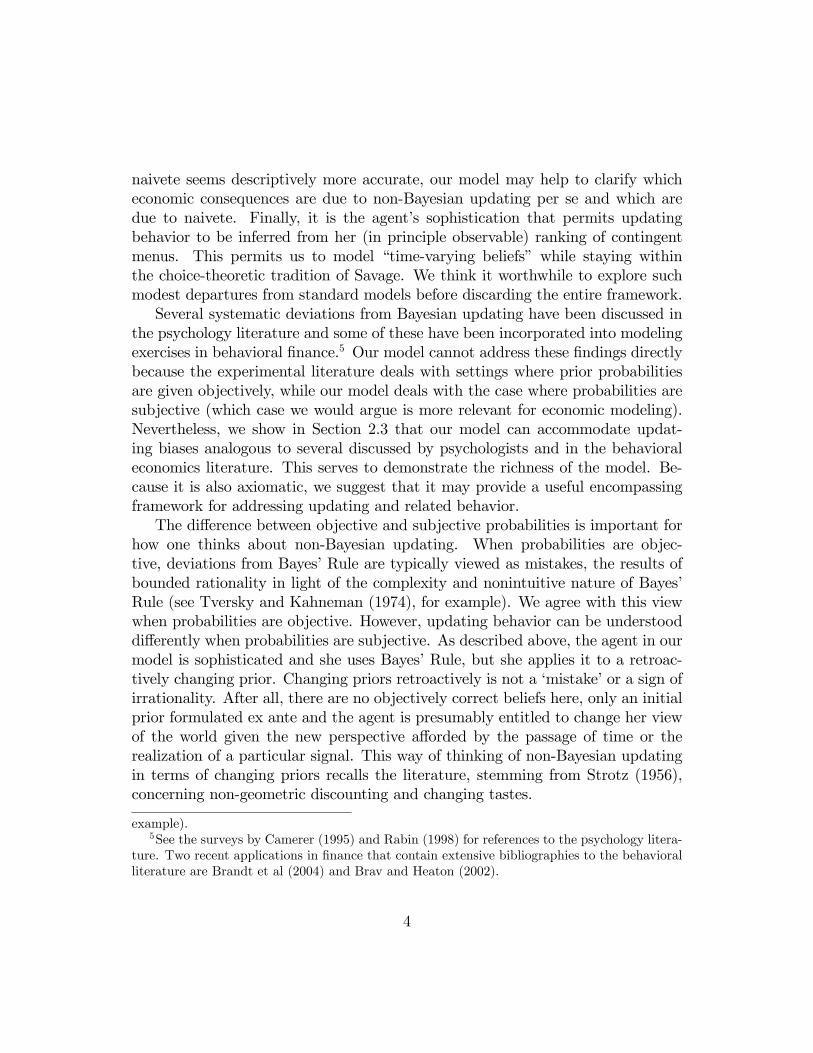
naivete seems descriptively more accurate, our model may help to clarify whicheconomic consequences are due to non-Bayesian updating per se and which aredue to naivete. Finally, it is the agent�s sophistication that permits updatingbehavior to be inferred from her (in principle observable) ranking of contingentmenus. This permits us to model �time-varying beliefs� while staying withinthe choice-theoretic tradition of Savage. We think it worthwhile to explore suchmodest departures from standard models before discarding the entire framework.Several systematic deviations from Bayesian updating have been discussed in

the psychology literature and some of these have been incorporated into modelingexercises in behavioral �nance.5 Our model cannot address these �ndings directlybecause the experimental literature deals with settings where prior probabilitiesare given objectively, while our model deals with the case where probabilities aresubjective (which case we would argue is more relevant for economic modeling).Nevertheless, we show in Section 2.3 that our model can accommodate updat-ing biases analogous to several discussed by psychologists and in the behavioraleconomics literature. This serves to demonstrate the richness of the model. Be-cause it is also axiomatic, we suggest that it may provide a useful encompassingframework for addressing updating and related behavior.The di¤erence between objective and subjective probabilities is important for

how one thinks about non-Bayesian updating. When probabilities are objec-tive, deviations from Bayes�Rule are typically viewed as mistakes, the results ofbounded rationality in light of the complexity and nonintuitive nature of Bayes�Rule (see Tversky and Kahneman (1974), for example). We agree with this viewwhen probabilities are objective. However, updating behavior can be understooddi¤erently when probabilities are subjective. As described above, the agent in ourmodel is sophisticated and she uses Bayes�Rule, but she applies it to a retroac-tively changing prior. Changing priors retroactively is not a �mistake�or a sign ofirrationality. After all, there are no objectively correct beliefs here, only an initialprior formulated ex ante and the agent is presumably entitled to change her viewof the world given the new perspective a¤orded by the passage of time or therealization of a particular signal. This way of thinking of non-Bayesian updatingin terms of changing priors recalls the literature, stemming from Strotz (1956),concerning non-geometric discounting and changing tastes.

example).5See the surveys by Camerer (1995) and Rabin (1998) for references to the psychology litera-

ture. Two recent applications in �nance that contain extensive bibliographies to the behavioralliterature are Brandt et al (2004) and Brav and Heaton (2002).

4

1.2. Updating, Temptation and Self-Control

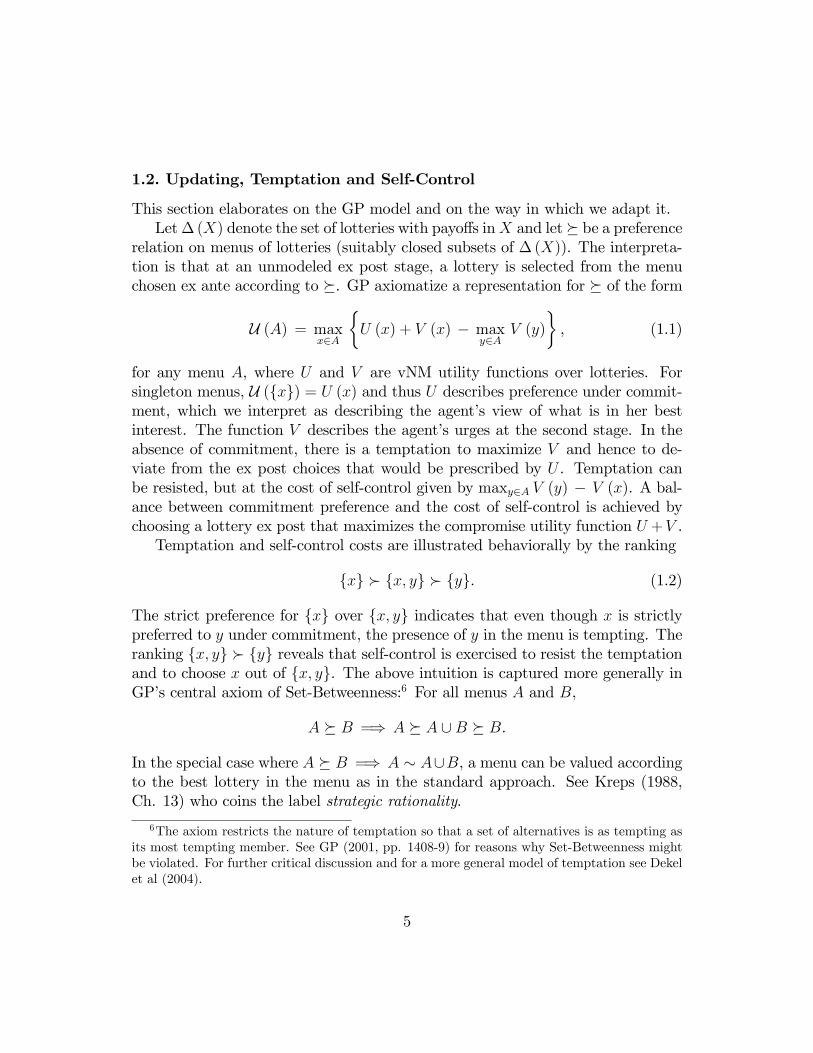
This section elaborates on the GP model and on the way in which we adapt it.Let�(X) denote the set of lotteries with payo¤s inX and let� be a preference

relation on menus of lotteries (suitably closed subsets of �(X)). The interpreta-tion is that at an unmodeled ex post stage, a lottery is selected from the menuchosen ex ante according to �. GP axiomatize a representation for � of the form

U (A) = maxx2A

�U (x) + V (x) � max

y2AV (y)

�, (1.1)

for any menu A, where U and V are vNM utility functions over lotteries. Forsingleton menus, U (fxg) = U (x) and thus U describes preference under commit-ment, which we interpret as describing the agent�s view of what is in her bestinterest. The function V describes the agent�s urges at the second stage. In theabsence of commitment, there is a temptation to maximize V and hence to de-viate from the ex post choices that would be prescribed by U . Temptation canbe resisted, but at the cost of self-control given by maxy2A V (y) � V (x). A bal-ance between commitment preference and the cost of self-control is achieved bychoosing a lottery ex post that maximizes the compromise utility function U +V .Temptation and self-control costs are illustrated behaviorally by the ranking

fxg � fx; yg � fyg. (1.2)

The strict preference for fxg over fx; yg indicates that even though x is strictlypreferred to y under commitment, the presence of y in the menu is tempting. Theranking fx; yg � fyg reveals that self-control is exercised to resist the temptationand to choose x out of fx; yg. The above intuition is captured more generally inGP�s central axiom of Set-Betweenness:6 For all menus A and B,

A � B =) A � A [B � B.

In the special case where A � B =) A � A[B, a menu can be valued accordingto the best lottery in the menu as in the standard approach. See Kreps (1988,Ch. 13) who coins the label strategic rationality.

6The axiom restricts the nature of temptation so that a set of alternatives is as tempting asits most tempting member. See GP (2001, pp. 1408-9) for reasons why Set-Betweenness mightbe violated. For further critical discussion and for a more general model of temptation see Dekelet al (2004).

5

The model to follow combines key elements of the GPmodel with the Anscombe-Aumann model of subjective probability. At a formal level, we introduce statespaces and consider preferences over (suitably contingent) menus of Anscombe-Aumann acts rather than over menus of lotteries. There are 3 periods - an exante stage 0, an interim period 1 when a signal s1 2 S1 is realized, and period 2when remaining uncertainty is resolved through realization of some s2 2 S2. Attime 0, the agent chooses some F , an s1-contingent menu of acts over S2. Shedoes this cognizant of the fact that at time 1, after a particular s1 is realized,she will update beliefs and then choose an act from the menu F (s1). Thus theway in which she updates will a¤ect the ultimate choice of an act and thereforealso the desirability at time 0 of any contingent menu. In this way, the natureof updating is revealed through preference over contingent menus. In particular,because non-Bayesian updating would lead to the �wrong�choice of an act fromthe menu after s1 is realized, the agent is led to value commitment at time 0.Under suitable axioms, we derive a representation for time 0 preference that

admits the following interpretation: there are two measures p and q, rather thana single measure as in Anscombe-Aumann and rather than two utility functionsas in (1.1). The signi�cance of p is that expected utility relative to p describespreferences under commitment. Therefore, p can be thought of as the counterpartof the Savage or Anscombe-Aumann prior. Updating does not play a role inthe ranking of contingent menus that provide commitment because these do notpermit any meaningful choice after realization of the signal. Suppose, however,that the agent faces a nonsingleton menu after seeing the signal s1 and considerthe factors in�uencing her choice of an act from the menu. In analogy withinterpretation of the GP functional form (1.1) given above, the second measure qrepresents the agent�s urges in the form of a retroactively new view of the worldat the interim stage. Her commitment view calls for choosing an act so as tomaximize conditional expected utility computed by applying Bayes�Rule to p,but she is tempted to act in accord with her new prior and to maximize expectedutility using the Bayesian update of q. In balancing these forces, she behaves asthough applying Bayes�Rule to a compromise measure p� that lies between p andq in a suitable sense: each s1-conditional of p� is a mixture of the conditionals ofp and q, where the mixture weights may vary with the signal s1. Consequently,interim choice out of the menu given s1 is based on the compromise posteriorp� (� j s1). If q and p di¤er, then so also do p� and p, and updating deviates fromapplication of Bayes�Rule to the commitment prior p.Note that temptation does not refer to whether or not to apply Bayes�Rule.

6

Rather, precisely as in GP, it refers to the temptation to follow one�s urges inmaking choices. The only di¤erence from GP is that here the con�ict is due tochanges in beliefs rather than in abstract utilities.For an illustration of some of the preceding, consider the following example

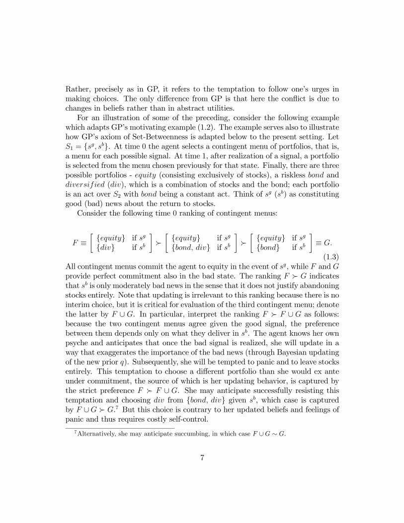
which adapts GP�s motivating example (1.2). The example serves also to illustratehow GP�s axiom of Set-Betweenness is adapted below to the present setting. LetS1 = fsg; sbg. At time 0 the agent selects a contingent menu of portfolios, that is,a menu for each possible signal. At time 1, after realization of a signal, a portfoliois selected from the menu chosen previously for that state. Finally, there are threepossible portfolios - equity (consisting exclusively of stocks), a riskless bond anddiversified (div), which is a combination of stocks and the bond; each portfoliois an act over S2 with bond being a constant act. Think of sg (sb) as constitutinggood (bad) news about the return to stocks.Consider the following time 0 ranking of contingent menus:

F ��fequityg if sg

fdivg if sb

���fequityg if sg

fbond; divg if sb

���fequityg if sg

fbondg if sb

�� G:

(1.3)All contingent menus commit the agent to equity in the event of sg, while F and Gprovide perfect commitment also in the bad state. The ranking F � G indicatesthat sb is only moderately bad news in the sense that it does not justify abandoningstocks entirely. Note that updating is irrelevant to this ranking because there is nointerim choice, but it is critical for evaluation of the third contingent menu; denotethe latter by F [ G. In particular, interpret the ranking F � F [ G as follows:because the two contingent menus agree given the good signal, the preferencebetween them depends only on what they deliver in sb. The agent knows her ownpsyche and anticipates that once the bad signal is realized, she will update in away that exaggerates the importance of the bad news (through Bayesian updatingof the new prior q). Subsequently, she will be tempted to panic and to leave stocksentirely. This temptation to choose a di¤erent portfolio than she would ex anteunder commitment, the source of which is her updating behavior, is captured bythe strict preference F � F [ G. She may anticipate successfully resisting thistemptation and choosing div from fbond; divg given sb, which case is capturedby F [G � G.7 But this choice is contrary to her updated beliefs and feelings ofpanic and thus requires costly self-control.

7Alternatively, she may anticipate succumbing, in which case F [G � G.

7

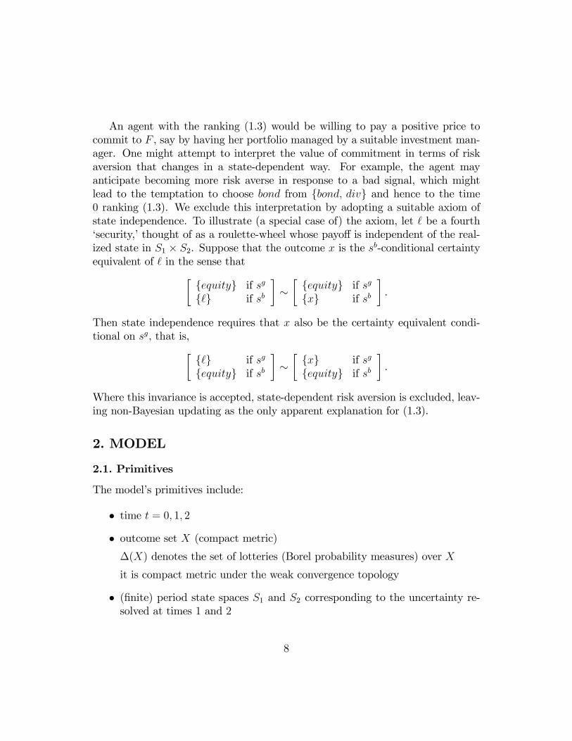
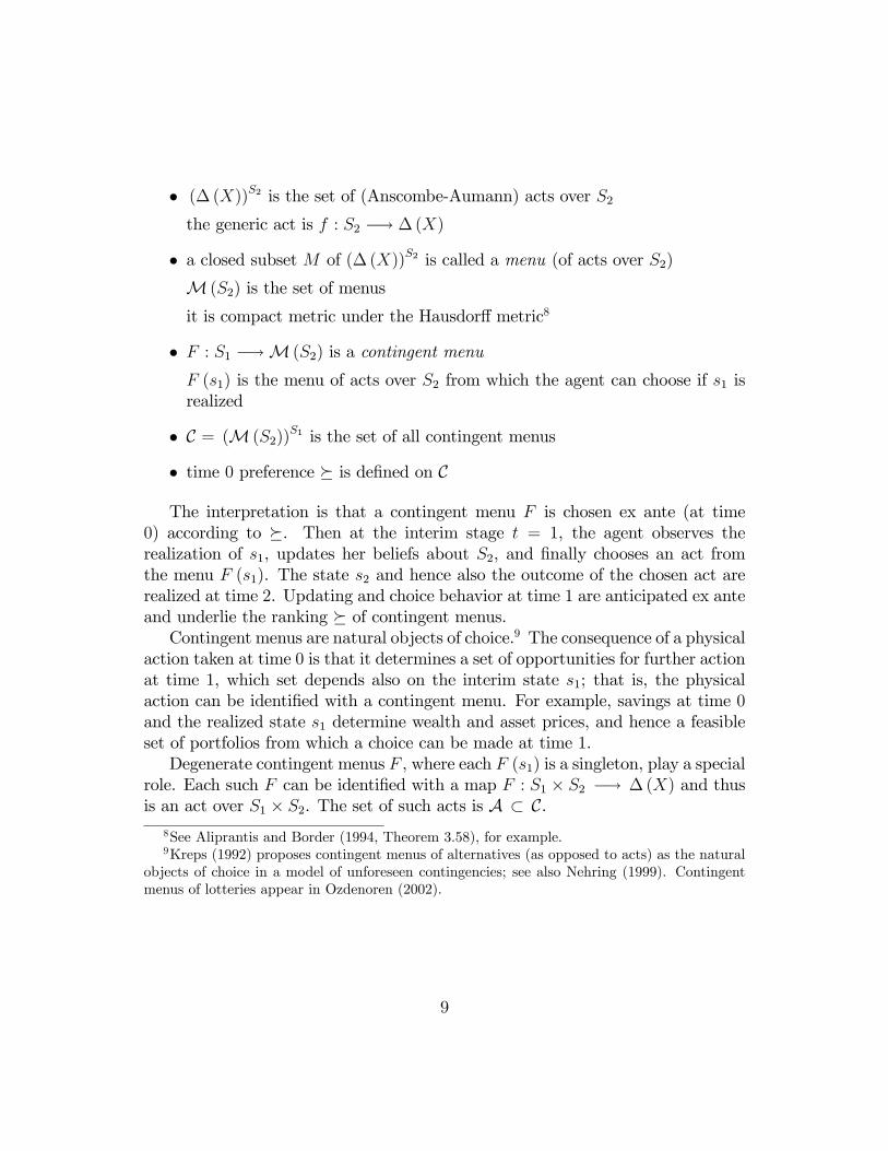
An agent with the ranking (1.3) would be willing to pay a positive price tocommit to F , say by having her portfolio managed by a suitable investment man-ager. One might attempt to interpret the value of commitment in terms of riskaversion that changes in a state-dependent way. For example, the agent mayanticipate becoming more risk averse in response to a bad signal, which mightlead to the temptation to choose bond from fbond; divg and hence to the time0 ranking (1.3). We exclude this interpretation by adopting a suitable axiom ofstate independence. To illustrate (a special case of) the axiom, let ` be a fourth�security,�thought of as a roulette-wheel whose payo¤ is independent of the real-ized state in S1 � S2. Suppose that the outcome x is the sb-conditional certaintyequivalent of ` in the sense that�

fequityg if sg

f`g if sb

���fequityg if sg

fxg if sb

�.

Then state independence requires that x also be the certainty equivalent condi-tional on sg, that is,�

f`g if sg

fequityg if sb

���fxg if sg

fequityg if sb

�.

Where this invariance is accepted, state-dependent risk aversion is excluded, leav-ing non-Bayesian updating as the only apparent explanation for (1.3).

2. MODEL

2.1. Primitives

The model�s primitives include:

� time t = 0; 1; 2

� outcome set X (compact metric)

�(X) denotes the set of lotteries (Borel probability measures) over X

it is compact metric under the weak convergence topology

� (�nite) period state spaces S1 and S2 corresponding to the uncertainty re-solved at times 1 and 2

8

� (� (X))S2 is the set of (Anscombe-Aumann) acts over S2

the generic act is f : S2 �! �(X)

� a closed subset M of (� (X))S2 is called a menu (of acts over S2)

M (S2) is the set of menus

it is compact metric under the Hausdor¤ metric8

� F : S1 �!M (S2) is a contingent menu

F (s1) is the menu of acts over S2 from which the agent can choose if s1 isrealized

� C = (M (S2))S1 is the set of all contingent menus

� time 0 preference � is de�ned on C

The interpretation is that a contingent menu F is chosen ex ante (at time0) according to �. Then at the interim stage t = 1, the agent observes therealization of s1, updates her beliefs about S2, and �nally chooses an act fromthe menu F (s1). The state s2 and hence also the outcome of the chosen act arerealized at time 2. Updating and choice behavior at time 1 are anticipated ex anteand underlie the ranking � of contingent menus.Contingent menus are natural objects of choice.9 The consequence of a physical

action taken at time 0 is that it determines a set of opportunities for further actionat time 1, which set depends also on the interim state s1; that is, the physicalaction can be identi�ed with a contingent menu. For example, savings at time 0and the realized state s1 determine wealth and asset prices, and hence a feasibleset of portfolios from which a choice can be made at time 1.Degenerate contingent menus F , where each F (s1) is a singleton, play a special

role. Each such F can be identi�ed with a map F : S1 � S2 �! �(X) and thusis an act over S1 � S2. The set of such acts is A � C.

8See Aliprantis and Border (1994, Theorem 3.58), for example.9Kreps (1992) proposes contingent menus of alternatives (as opposed to acts) as the natural

objects of choice in a model of unforeseen contingencies; see also Nehring (1999). Contingentmenus of lotteries appear in Ozdenoren (2002).

9

2.2. Utility

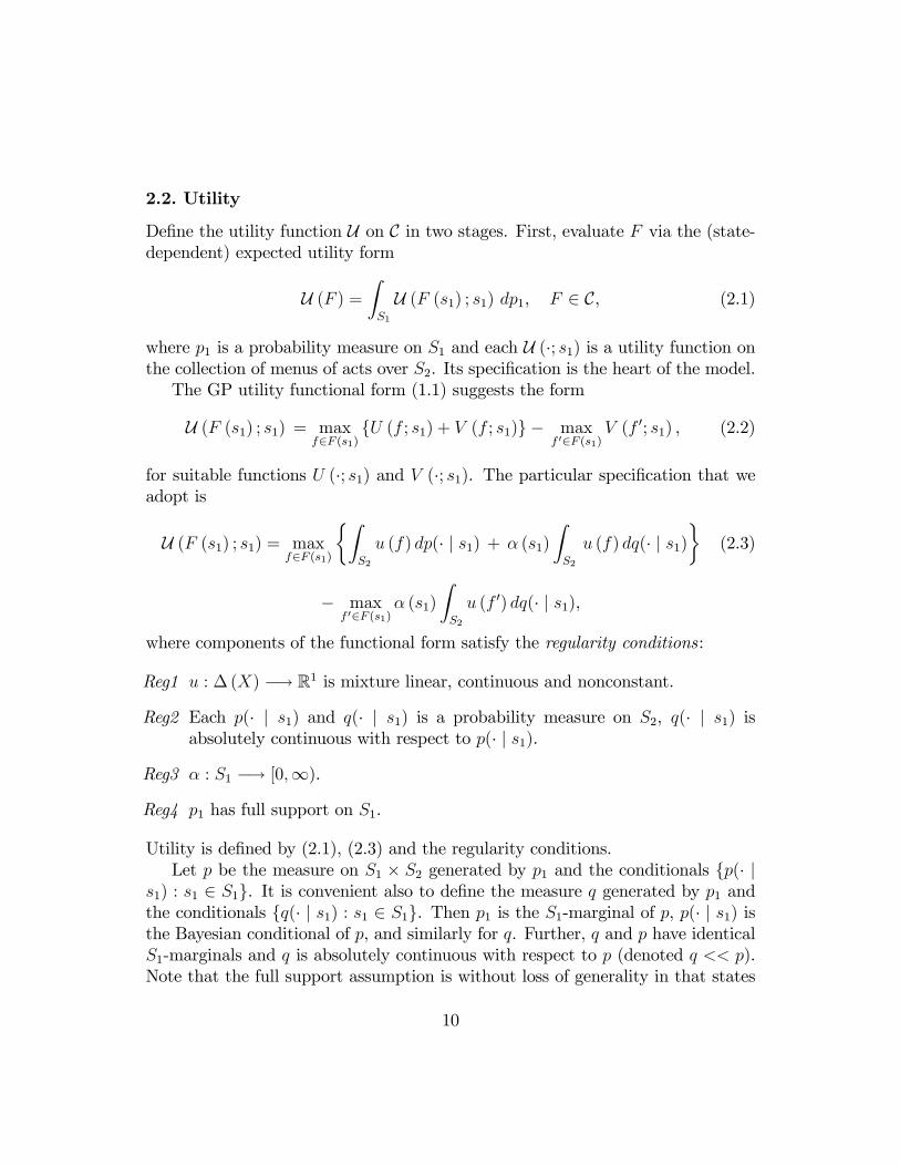
De�ne the utility function U on C in two stages. First, evaluate F via the (state-dependent) expected utility form

U (F ) =ZS1

U (F (s1) ; s1) dp1, F 2 C, (2.1)

where p1 is a probability measure on S1 and each U (�; s1) is a utility function onthe collection of menus of acts over S2. Its speci�cation is the heart of the model.The GP utility functional form (1.1) suggests the form

U (F (s1) ; s1) = maxf2F (s1)

fU (f ; s1) + V (f ; s1)g � maxf 02F (s1)

V (f 0; s1) , (2.2)

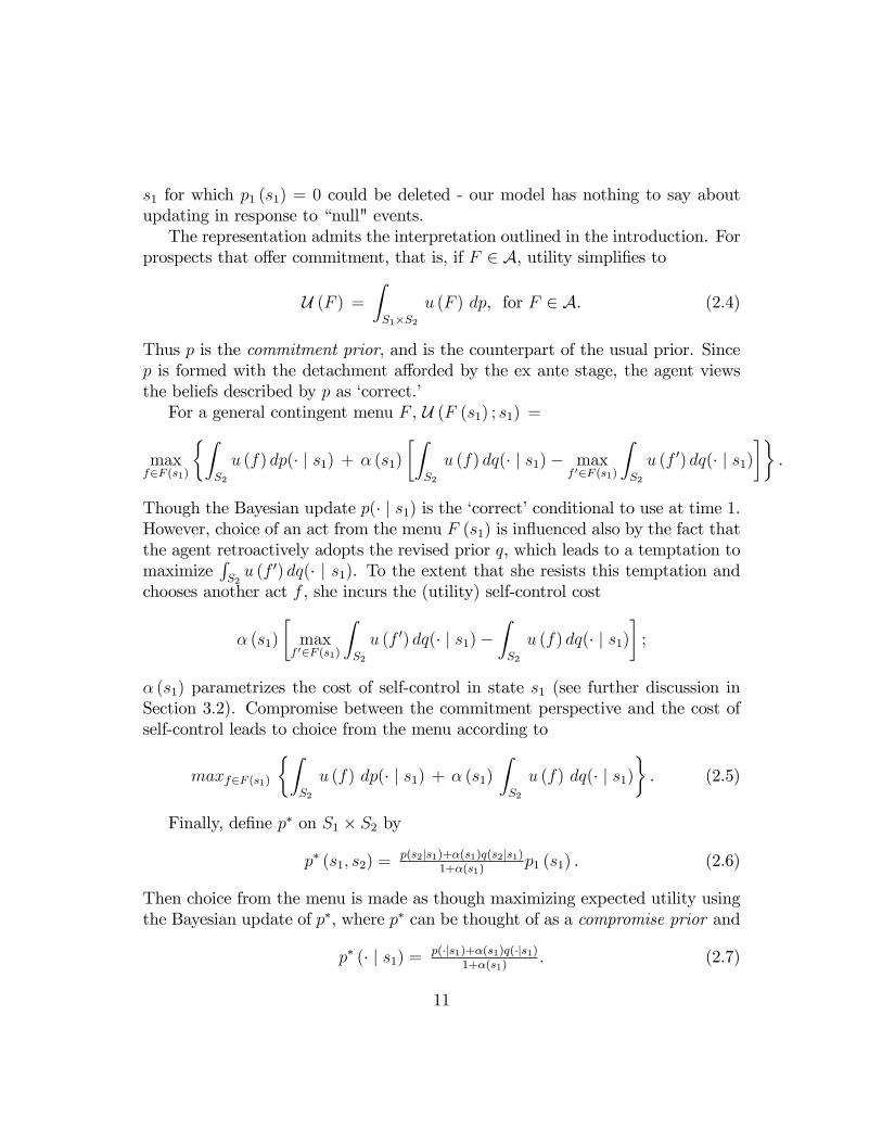
for suitable functions U (�; s1) and V (�; s1). The particular speci�cation that weadopt is

U (F (s1) ; s1) = maxf2F (s1)

�ZS2

u (f) dp(� j s1) + � (s1)

ZS2

u (f) dq(� j s1)�

(2.3)

� maxf 02F (s1)

� (s1)

ZS2

u (f 0) dq(� j s1),

where components of the functional form satisfy the regularity conditions:

Reg1 u : � (X) �! R1 is mixture linear, continuous and nonconstant.

Reg2 Each p(� j s1) and q(� j s1) is a probability measure on S2, q(� j s1) isabsolutely continuous with respect to p(� j s1).

Reg3 � : S1 �! [0;1).

Reg4 p1 has full support on S1.

Utility is de�ned by (2.1), (2.3) and the regularity conditions.Let p be the measure on S1 � S2 generated by p1 and the conditionals fp(� j

s1) : s1 2 S1g. It is convenient also to de�ne the measure q generated by p1 andthe conditionals fq(� j s1) : s1 2 S1g. Then p1 is the S1-marginal of p, p(� j s1) isthe Bayesian conditional of p, and similarly for q. Further, q and p have identicalS1-marginals and q is absolutely continuous with respect to p (denoted q << p).Note that the full support assumption is without loss of generality in that states

10

s1 for which p1 (s1) = 0 could be deleted - our model has nothing to say aboutupdating in response to �null" events.The representation admits the interpretation outlined in the introduction. For

prospects that o¤er commitment, that is, if F 2 A, utility simpli�es to

U (F ) =ZS1�S2

u (F ) dp, for F 2 A. (2.4)

Thus p is the commitment prior, and is the counterpart of the usual prior. Sincep is formed with the detachment a¤orded by the ex ante stage, the agent viewsthe beliefs described by p as �correct.�For a general contingent menu F , U (F (s1) ; s1) =

maxf2F (s1)

�ZS2

u (f) dp(� j s1) + � (s1)

�ZS2

u (f) dq(� j s1)� maxf 02F (s1)

ZS2

u (f 0) dq(� j s1)��.

Though the Bayesian update p(� j s1) is the �correct�conditional to use at time 1.However, choice of an act from the menu F (s1) is in�uenced also by the fact thatthe agent retroactively adopts the revised prior q, which leads to a temptation tomaximize

RS2u (f 0) dq(� j s1). To the extent that she resists this temptation and

chooses another act f , she incurs the (utility) self-control cost

� (s1)

�max

f 02F (s1)

ZS2

u (f 0) dq(� j s1)�ZS2

u (f) dq(� j s1)�;

� (s1) parametrizes the cost of self-control in state s1 (see further discussion inSection 3.2). Compromise between the commitment perspective and the cost ofself-control leads to choice from the menu according to

maxf2F (s1)

�ZS2

u (f) dp(� j s1) + � (s1)

ZS2

u (f) dq(� j s1)�. (2.5)

Finally, de�ne p� on S1 � S2 by

p� (s1; s2) =p(s2js1)+�(s1)q(s2js1)

1+�(s1)p1 (s1) . (2.6)

Then choice from the menu is made as though maximizing expected utility usingthe Bayesian update of p�, where p� can be thought of as a compromise prior and

p� (� j s1) = p(�js1)+�(s1)q(�js1)1+�(s1)

: (2.7)

11

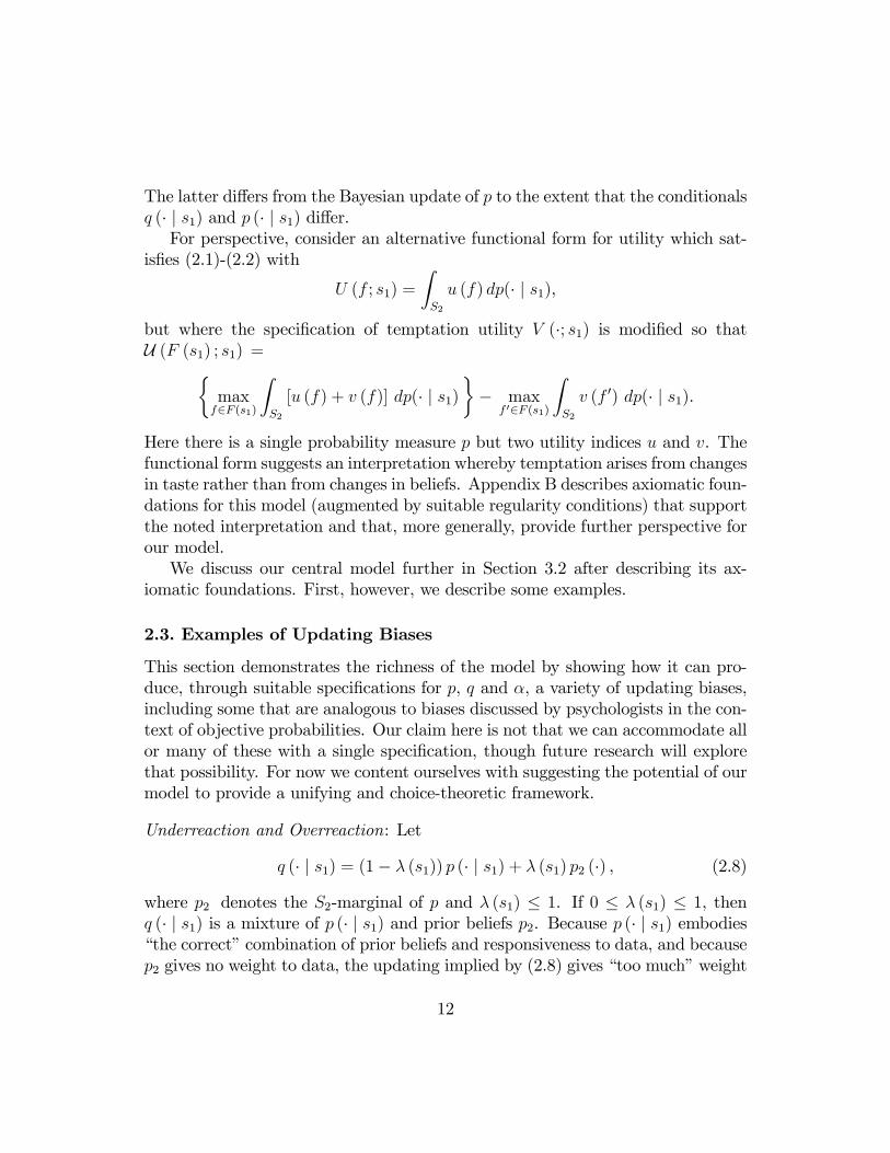
The latter di¤ers from the Bayesian update of p to the extent that the conditionalsq (� j s1) and p (� j s1) di¤er.For perspective, consider an alternative functional form for utility which sat-

is�es (2.1)-(2.2) with

U (f ; s1) =

ZS2

u (f) dp(� j s1),

but where the speci�cation of temptation utility V (�; s1) is modi�ed so thatU (F (s1) ; s1) =�

maxf2F (s1)

ZS2

[u (f) + v (f)] dp(� j s1)�� max

f 02F (s1)

ZS2

v (f 0) dp(� j s1).

Here there is a single probability measure p but two utility indices u and v. Thefunctional form suggests an interpretation whereby temptation arises from changesin taste rather than from changes in beliefs. Appendix B describes axiomatic foun-dations for this model (augmented by suitable regularity conditions) that supportthe noted interpretation and that, more generally, provide further perspective forour model.We discuss our central model further in Section 3.2 after describing its ax-

iomatic foundations. First, however, we describe some examples.

2.3. Examples of Updating Biases

This section demonstrates the richness of the model by showing how it can pro-duce, through suitable speci�cations for p, q and �, a variety of updating biases,including some that are analogous to biases discussed by psychologists in the con-text of objective probabilities. Our claim here is not that we can accommodate allor many of these with a single speci�cation, though future research will explorethat possibility. For now we content ourselves with suggesting the potential of ourmodel to provide a unifying and choice-theoretic framework.

Underreaction and Overreaction: Let

q (� j s1) = (1� � (s1)) p (� j s1) + � (s1) p2 (�) , (2.8)

where p2 denotes the S2-marginal of p and � (s1) � 1. If 0 � � (s1) � 1, thenq (� j s1) is a mixture of p (� j s1) and prior beliefs p2. Because p (� j s1) embodies�the correct�combination of prior beliefs and responsiveness to data, and becausep2 gives no weight to data, the updating implied by (2.8) gives �too much�weight

12

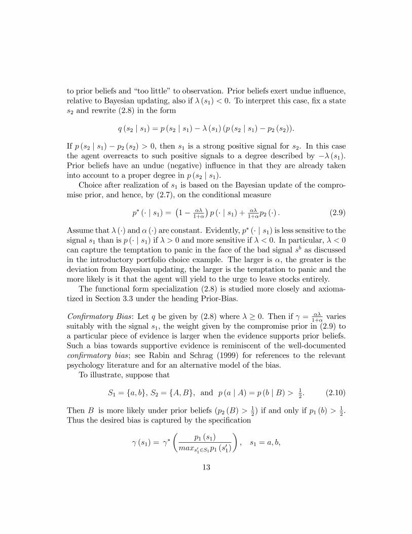
to prior beliefs and �too little�to observation. Prior beliefs exert undue in�uence,relative to Bayesian updating, also if � (s1) < 0. To interpret this case, �x a states2 and rewrite (2.8) in the form

q (s2 j s1) = p (s2 j s1)� � (s1) (p (s2 j s1)� p2 (s2)).

If p (s2 j s1) � p2 (s2) > 0, then s1 is a strong positive signal for s2. In this casethe agent overreacts to such positive signals to a degree described by �� (s1).Prior beliefs have an undue (negative) in�uence in that they are already takeninto account to a proper degree in p (s2 j s1).Choice after realization of s1 is based on the Bayesian update of the compro-

mise prior, and hence, by (2.7), on the conditional measure

p� (� j s1) =�1� ��

1+�

�p (� j s1) + ��

1+�p2 (�) : (2.9)

Assume that � (�) and � (�) are constant. Evidently, p� (� j s1) is less sensitive to thesignal s1 than is p (� j s1) if � > 0 and more sensitive if � < 0. In particular, � < 0can capture the temptation to panic in the face of the bad signal sb as discussedin the introductory portfolio choice example. The larger is �, the greater is thedeviation from Bayesian updating, the larger is the temptation to panic and themore likely is it that the agent will yield to the urge to leave stocks entirely.The functional form specialization (2.8) is studied more closely and axioma-

tized in Section 3.3 under the heading Prior-Bias.

Con�rmatory Bias: Let q be given by (2.8) where � � 0. Then if = ��1+�

variessuitably with the signal s1, the weight given by the compromise prior in (2.9) toa particular piece of evidence is larger when the evidence supports prior beliefs.Such a bias towards supportive evidence is reminiscent of the well-documentedcon�rmatory bias; see Rabin and Schrag (1999) for references to the relevantpsychology literature and for an alternative model of the bias.To illustrate, suppose that

S1 = fa; bg, S2 = fA;Bg, and p (a j A) = p (b j B) > 12. (2.10)

Then B is more likely under prior beliefs (p2 (B) > 12) if and only if p1 (b) > 1

2.

Thus the desired bias is captured by the speci�cation

(s1) = ��

p1 (s1)

maxs012S1p1 (s01)

�, s1 = a; b,

13

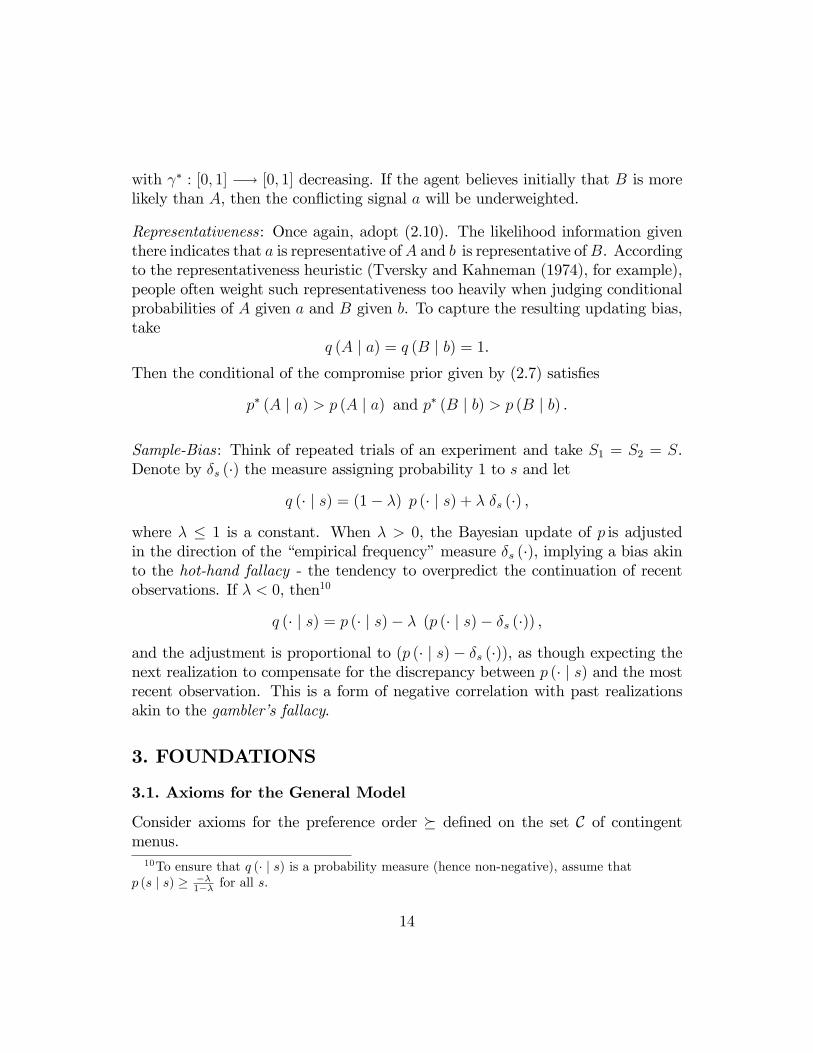
with � : [0; 1] �! [0; 1] decreasing. If the agent believes initially that B is morelikely than A, then the con�icting signal a will be underweighted.

Representativeness: Once again, adopt (2.10). The likelihood information giventhere indicates that a is representative ofA and b is representative ofB. Accordingto the representativeness heuristic (Tversky and Kahneman (1974), for example),people often weight such representativeness too heavily when judging conditionalprobabilities of A given a and B given b. To capture the resulting updating bias,take

q (A j a) = q (B j b) = 1.Then the conditional of the compromise prior given by (2.7) satis�es

p� (A j a) > p (A j a) and p� (B j b) > p (B j b) .

Sample-Bias: Think of repeated trials of an experiment and take S1 = S2 = S.Denote by �s (�) the measure assigning probability 1 to s and let

q (� j s) = (1� �) p (� j s) + � �s (�) ,

where � � 1 is a constant. When � > 0, the Bayesian update of p is adjustedin the direction of the �empirical frequency�measure �s (�), implying a bias akinto the hot-hand fallacy - the tendency to overpredict the continuation of recentobservations. If � < 0, then10

q (� j s) = p (� j s)� � (p (� j s)� �s (�)) ,

and the adjustment is proportional to (p (� j s)� �s (�)), as though expecting thenext realization to compensate for the discrepancy between p (� j s) and the mostrecent observation. This is a form of negative correlation with past realizationsakin to the gambler�s fallacy.

3. FOUNDATIONS

3.1. Axioms for the General Model

Consider axioms for the preference order � de�ned on the set C of contingentmenus.10To ensure that q (� j s) is a probability measure (hence non-negative), assume that

p (s j s) � ��1�� for all s.

14

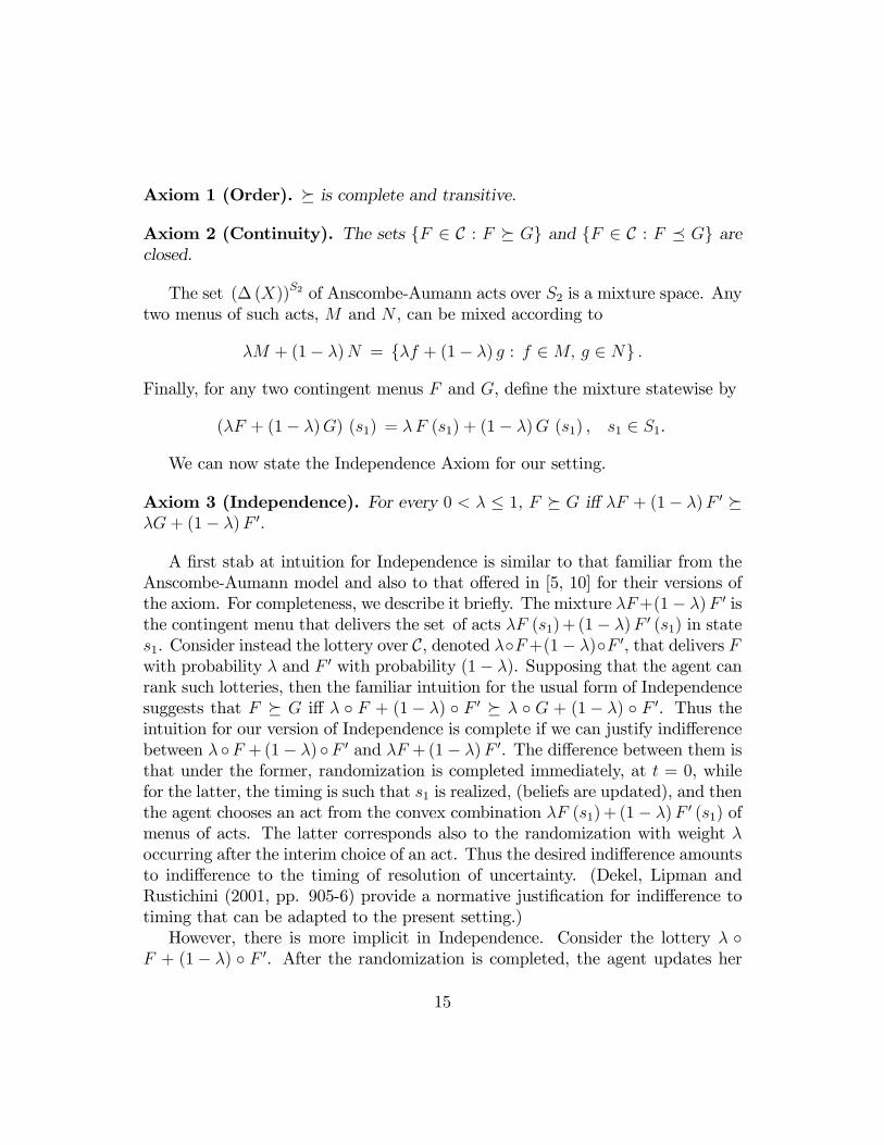
Axiom 1 (Order). � is complete and transitive.

Axiom 2 (Continuity). The sets fF 2 C : F � Gg and fF 2 C : F � Gg areclosed.

The set (� (X))S2 of Anscombe-Aumann acts over S2 is a mixture space. Anytwo menus of such acts, M and N , can be mixed according to

�M + (1� �)N = f�f + (1� �) g : f 2M; g 2 Ng :

Finally, for any two contingent menus F and G, de�ne the mixture statewise by

(�F + (1� �)G) (s1) = �F (s1) + (1� �)G (s1) , s1 2 S1.

We can now state the Independence Axiom for our setting.

Axiom 3 (Independence). For every 0 < � � 1, F � G i¤ �F + (1� �)F 0 ��G+ (1� �)F 0.

A �rst stab at intuition for Independence is similar to that familiar from theAnscombe-Aumann model and also to that o¤ered in [5, 10] for their versions ofthe axiom. For completeness, we describe it brie�y. The mixture �F+(1� �)F 0 isthe contingent menu that delivers the set of acts �F (s1)+ (1� �)F 0 (s1) in states1. Consider instead the lottery over C, denoted ��F+(1� �)�F 0, that delivers Fwith probability � and F 0 with probability (1� �). Supposing that the agent canrank such lotteries, then the familiar intuition for the usual form of Independencesuggests that F � G i¤ � � F + (1� �) � F 0 � � � G + (1� �) � F 0. Thus theintuition for our version of Independence is complete if we can justify indi¤erencebetween � �F +(1� �) �F 0 and �F +(1� �)F 0. The di¤erence between them isthat under the former, randomization is completed immediately, at t = 0, whilefor the latter, the timing is such that s1 is realized, (beliefs are updated), and thenthe agent chooses an act from the convex combination �F (s1)+ (1� �)F 0 (s1) ofmenus of acts. The latter corresponds also to the randomization with weight �occurring after the interim choice of an act. Thus the desired indi¤erence amountsto indi¤erence to the timing of resolution of uncertainty. (Dekel, Lipman andRustichini (2001, pp. 905-6) provide a normative justi�cation for indi¤erence totiming that can be adapted to the present setting.)However, there is more implicit in Independence. Consider the lottery � �

F + (1� �) � F 0. After the randomization is completed, the agent updates her

15

beliefs over S1 � S2. Though the randomization is objectively independent ofevents in S1 � S2, given that she changes her view of the world after making anobservation, the agent might change her beliefs over S1�S2. As a result, she mightprefer � � G + (1� �) � F 0 to � � F + (1� �) � F 0 even while preferring F to G.Thus intuition for Independence assumes that, consistent with our agent not beingone who makes mistakes, she recognizes the objective fact that randomization isunrelated to the state space. At the same time, she may, according to our model,view the events E1 � S1 and E2 � S2 as subjectively independent according toher initial (commitment) prior and yet change her beliefs about E2 after seeingE1.To rule out trivial cases, adopt:11

Axiom 4 (Nondegeneracy). There exist x; y in X for which x � y.

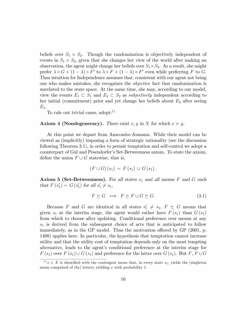
At this point we depart from Anscombe-Aumann. While their model can beviewed as (implicitly) imposing a form of strategic rationality (see the discussionfollowing Theorem 3.1), in order to permit temptation and self-control we adopt acounterpart of Gul and Pesendorfer�s Set-Betweenness axiom. To state the axiom,de�ne the union F [G statewise, that is,

(F [G) (s1) = F (s1) [ G (s1) .

Axiom 5 (Set-Betweenness). For all states s1 and all menus F and G suchthat F (s01) = G (s01) for all s

01 6= s1,

F � G =) F � F [G � G. (3.1)

Because F and G are identical in all states s01 6= s1, F � G means thatgiven s1 at the interim stage, the agent would rather have F (s1) than G (s1)from which to choose after updating. Conditional preference over menus at anys1 is derived from the subsequent choice of acts that is anticipated to followimmediately, as in the GP model. Thus the motivation o¤ered by GP (2001, p.1408) applies here. In particular, the hypothesis that temptation cannot increaseutility and that the utility cost of temptation depends only on the most temptingalternative, leads to the agent�s conditional preference at the interim stage forF (s1) over F (s1)[ G (s1) and preference for the latter over G (s1). But F , F [G11x 2 X is identi�ed with the contingent menu that, in every state s1, yields the (singleton

menu comprised of the) lottery yielding x with probability 1.

16

and G coincide in all states s01 6= s1 and thus, from the ex ante perspective, thedesired ranking of F [ G follows. The portfolio choice example (1.3) illustratesthe preceding.For perspective, consider the stronger axiom that would impose (3.1) for all

contingent menus and not just for those that di¤er only in one state s1. It is easilyseen that this stronger axiom is not intuitive.12 For example, suppose that

F ��ffg if s1ff 0g if s01

���fgg if s1fg0g if s01

�� G,

where f and g0 are very attractive acts over S2 while f 0 and g are less attractivebut suitably tempting. Suppose that

ffg �s1 ff; gg �s1 fgg and

fg0g �s01 ff0; g0g �s01 ff

0g,where �s1 and �s01 denote preference at the interim stage given realization of s1and s01 respectively. In particular, g is so tempting given s1 that it would bechosen out of ff; gg, and f 0 is so tempting given s01 that it would be chosen out offf 0; g0g. Therefore, F [ G would lead ultimately to the choice of g given s1 andf 0 given s01, the worst of both worlds, which suggests the ranking G � F [G.The next axiom is the principal way in which temptation is connected to

changing beliefs. At the functional form level, the axiom is important in tracingthe di¤erence between the counterparts of the two GP functions U and V in (1.1)to di¤erences in beliefs rather than to di¤erences in risk attitudes or utilities over�nal outcomes (see Appendix B).Identify any menu of lotteries L � �(X) with the contingent menu that yields

L for every s1. Thus rankings of the form L0 � L are well-de�ned.

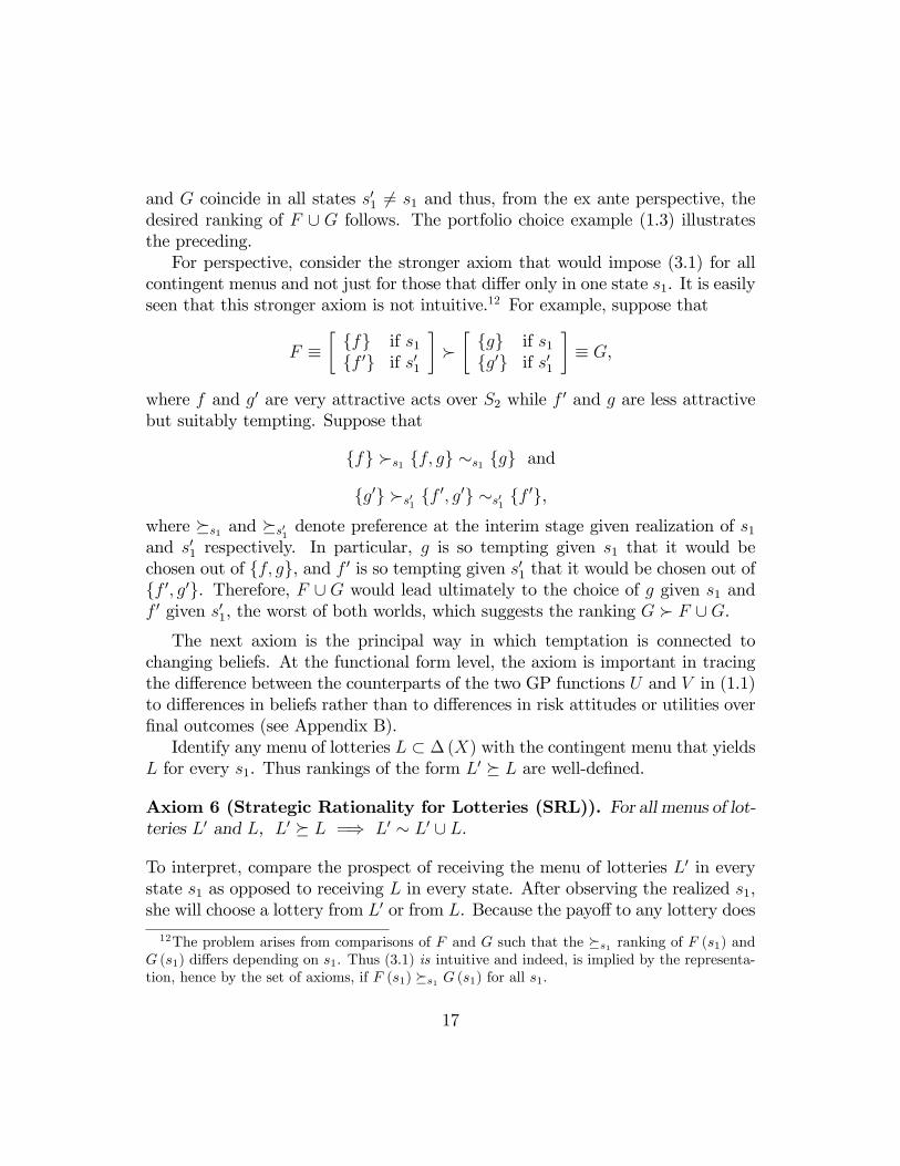
Axiom 6 (Strategic Rationality for Lotteries (SRL)). For all menus of lot-teries L0 and L, L0 � L =) L0 � L0 [ L.

To interpret, compare the prospect of receiving the menu of lotteries L0 in everystate s1 as opposed to receiving L in every state. After observing the realized s1,she will choose a lottery from L0 or from L. Because the payo¤ to any lottery does

12The problem arises from comparisons of F and G such that the �s1 ranking of F (s1) andG (s1) di¤ers depending on s1. Thus (3.1) is intuitive and indeed, is implied by the representa-tion, hence by the set of axioms, if F (s1) �s1 G (s1) for all s1.

17

not depend on the ultimate state s2, the expected payo¤ at the interim stage doesnot depend on beliefs about S2. Therefore, if temptations arise only with a changein beliefs, a form of strategic rationality should be valid for such comparisons.

The sequel requires a notion of nullity and some added notation that we nowintroduce. For any act f over S2 and state s2 in S2, denote by f�s2 the restrictionof f to S2nfs2g. Say that (s1; s2) is null if F 0 � F for all F 0 and F satisfying both

F 0 (s01) = F (s01) for all s01 6= s1, and�

f 0�s2 : f0 2 F 0 (s1)

= ff�s2 : f 2 F (s1)g .

In words, (s1; s2) is null if any two contingent menus that �di¤er only on (s1; s2)�are indi¤erent.For any act f over S2, lottery ` and state s2, denote by `s2f the act over S2

that assigns ` if the realized state is s2 and f (s02) if the realized state is s02 6= s2.

Similarly, for any menu M 2M (S2) and menu of lotteries L � �(X),

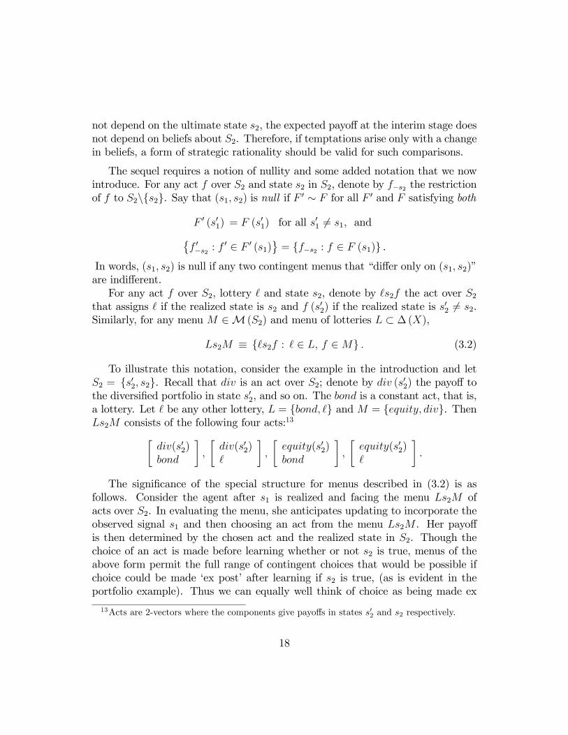
Ls2M � f`s2f : ` 2 L; f 2Mg : (3.2)

To illustrate this notation, consider the example in the introduction and letS2 = fs02; s2g. Recall that div is an act over S2; denote by div (s02) the payo¤ tothe diversi�ed portfolio in state s02, and so on. The bond is a constant act, that is,a lottery. Let ` be any other lottery, L = fbond; `g and M = fequity; divg. ThenLs2M consists of the following four acts:13�

div(s02)bond

�;

�div(s02)`

�;

�equity(s02)bond

�;

�equity(s02)`

�.

The signi�cance of the special structure for menus described in (3.2) is asfollows. Consider the agent after s1 is realized and facing the menu Ls2M ofacts over S2. In evaluating the menu, she anticipates updating to incorporate theobserved signal s1 and then choosing an act from the menu Ls2M . Her payo¤is then determined by the chosen act and the realized state in S2. Though thechoice of an act is made before learning whether or not s2 is true, menus of theabove form permit the full range of contingent choices that would be possible ifchoice could be made �ex post�after learning if s2 is true, (as is evident in theportfolio example). Thus we can equally well think of choice as being made ex

13Acts are 2-vectors where the components give payo¤s in states s02 and s2 respectively.

18

post and of the agent as having the following perspective: if s2 is realized, thenI will choose a lottery from L, and if s2 is not realized, then I will choose an actfrom M . Similarly when evaluating L0s2M . Thus when comparing L0s2M andLs2M , the usual intuition for separability across disjoint events suggests that thecomparison reduces to the question �given state s2, would I rather choose a lotteryfrom L0 or from L?�Finally, denote by (F�s1 ; Ls2M) the contingent menu that delivers F (s

01) if

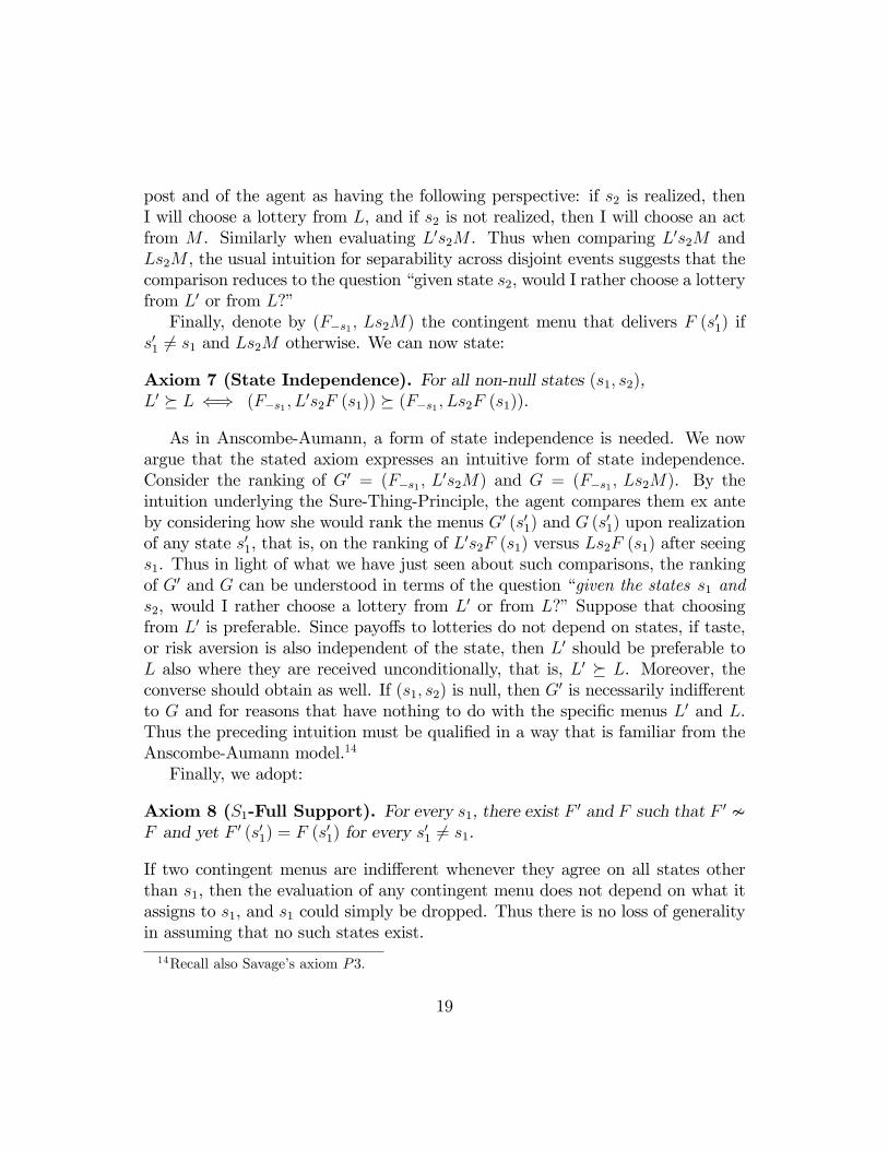
s01 6= s1 and Ls2M otherwise. We can now state:

Axiom 7 (State Independence). For all non-null states (s1; s2),L0 � L () (F�s1 ; L

0s2F (s1)) � (F�s1 ; Ls2F (s1)).

As in Anscombe-Aumann, a form of state independence is needed. We nowargue that the stated axiom expresses an intuitive form of state independence.Consider the ranking of G0 = (F�s1 ; L

0s2M) and G = (F�s1 ; Ls2M). By theintuition underlying the Sure-Thing-Principle, the agent compares them ex anteby considering how she would rank the menus G0 (s01) and G (s

01) upon realization

of any state s01, that is, on the ranking of L0s2F (s1) versus Ls2F (s1) after seeing

s1. Thus in light of what we have just seen about such comparisons, the rankingof G0 and G can be understood in terms of the question �given the states s1 ands2, would I rather choose a lottery from L0 or from L?�Suppose that choosingfrom L0 is preferable. Since payo¤s to lotteries do not depend on states, if taste,or risk aversion is also independent of the state, then L0 should be preferable toL also where they are received unconditionally, that is, L0 � L. Moreover, theconverse should obtain as well. If (s1; s2) is null, then G0 is necessarily indi¤erentto G and for reasons that have nothing to do with the speci�c menus L0 and L.Thus the preceding intuition must be quali�ed in a way that is familiar from theAnscombe-Aumann model.14

Finally, we adopt:

Axiom 8 (S1-Full Support). For every s1, there exist F 0 and F such that F 0 �F and yet F 0 (s01) = F (s

01) for every s

01 6= s1.

If two contingent menus are indi¤erent whenever they agree on all states otherthan s1, then the evaluation of any contingent menu does not depend on what itassigns to s1, and s1 could simply be dropped. Thus there is no loss of generalityin assuming that no such states exist.

14Recall also Savage�s axiom P3.

19

3.2. Representation Result

The central result of the paper is the following axiomatization of utility overcontingent menus:

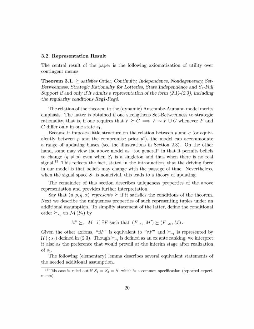
Theorem 3.1. � satis�es Order, Continuity, Independence, Nondegeneracy, Set-Betweenness, Strategic Rationality for Lotteries, State Independence and S1-FullSupport if and only if it admits a representation of the form (2.1)-(2.3), includingthe regularity conditions Reg1-Reg4.

The relation of the theorem to the (dynamic) Anscombe-Aumann model meritsemphasis. The latter is obtained if one strengthens Set-Betweenness to strategicrationality, that is, if one requires that F � G =) F � F [ G whenever F andG di¤er only in one state s1.Because it imposes little structure on the relation between p and q (or equiv-

alently between p and the compromise prior p�), the model can accommodatea range of updating biases (see the illustrations in Section 2.3). On the otherhand, some may view the above model as �too general�in that it permits beliefsto change (q 6= p) even when S1 is a singleton and thus when there is no realsignal.15 This re�ects the fact, stated in the introduction, that the driving forcein our model is that beliefs may change with the passage of time. Nevertheless,when the signal space S1 is nontrivial, this leads to a theory of updating.

The remainder of this section describes uniqueness properties of the aboverepresentation and provides further interpretation.Say that (u; p; q; �) represents � if it satis�es the conditions of the theorem.

Next we describe the uniqueness properties of such representing tuples under anadditional assumption. To simplify statement of the latter, de�ne the conditionalorder �s1 onM (S2) by

M 0 �s1 M if 9F such that (F�s1 ;M 0) � (F�s1 ;M) .

Given the other axioms, �9F� is equivalent to �8F�and �s1 is represented byU (�; s1) de�ned in (2.3). Though �s1 is de�ned as an ex ante ranking, we interpretit also as the preference that would prevail at the interim stage after realizationof s1.The following (elementary) lemma describes several equivalent statements of

the needed additional assumption.15This case is ruled out if S1 = S2 = S, which is a common speci�cation (repeated experi-

ments).

20

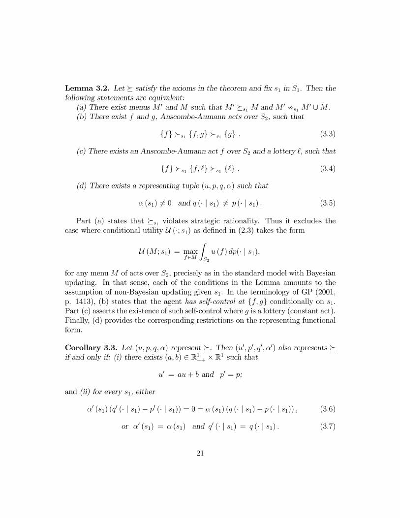
Lemma 3.2. Let � satisfy the axioms in the theorem and �x s1 in S1. Then thefollowing statements are equivalent:(a) There exist menus M 0 and M such that M 0 �s1 M and M 0 �s1 M 0 [M .(b) There exist f and g, Anscombe-Aumann acts over S2, such that

ffg �s1 ff; gg �s1 fgg . (3.3)

(c) There exists an Anscombe-Aumann act f over S2 and a lottery `, such that

ffg �s1 ff; `g �s1 f`g . (3.4)

(d) There exists a representing tuple (u; p; q; �) such that

� (s1) 6= 0 and q (� j s1) 6= p (� j s1) . (3.5)

Part (a) states that �s1 violates strategic rationality. Thus it excludes thecase where conditional utility U (�; s1) as de�ned in (2.3) takes the form

U (M ; s1) = maxf2M

ZS2

u (f) dp(� j s1),

for any menuM of acts over S2, precisely as in the standard model with Bayesianupdating. In that sense, each of the conditions in the Lemma amounts to theassumption of non-Bayesian updating given s1. In the terminology of GP (2001,p. 1413), (b) states that the agent has self-control at ff; gg conditionally on s1.Part (c) asserts the existence of such self-control where g is a lottery (constant act).Finally, (d) provides the corresponding restrictions on the representing functionalform.

Corollary 3.3. Let (u; p; q; �) represent �. Then (u0; p0; q0; �0) also represents �if and only if: (i) there exists (a; b) 2 R1++ � R1 such that

u0 = au+ b and p0 = p;

and (ii) for every s1, either

�0 (s1) (q0 (� j s1)� p0 (� j s1)) = 0 = � (s1) (q (� j s1)� p (� j s1)) , (3.6)

or �0 (s1) = � (s1) and q0 (� j s1) = q (� j s1) : (3.7)

21

The uniqueness properties of (u; p) are straightforward and expected. For (q; �),the relevant uniqueness property depends on s1. One possibility is (3.6) whichstates that both representations violate condition (3.5). In that case, interimchoice behavior is based on the Bayesian update of p. Otherwise, the stronguniqueness statement (3.7) is valid for s1.If conditions of the Lemma are satis�ed for every s1, then (u0; p0; q0; �0) and

(u; p; q; �) both represent � if and only if

u0 = au+ b and (p0; q0; �0) = (p; q; �) ,

for some a > 0 and b 2 R1. Then q and � (�), in addition to p, are uniqueand hence meaningful components of the functional form. It makes sense then toconsider their behavioral meaning. For p, we have already observed that it is theprior that guides choice under commitment. The meaning of � can be describedexplicitly under conditions of the Lemma as we now show.16

Let x�� and x� be best and worst alternatives under commitment, that is, suchthat

fx��g � fxg � fx�g for all x in X.

(They exist by Continuity and compactness of X.) Then also

fx��g �s1 M �s1 fx�g

for all states s1 and menus M . Normalizing u so that

u (x��) = 1 and u (x�) = 0,

then, as in vNM theory, utilities are directly observable as �mixture weights�. Thatis, because each U (�; s1) is mixture linear, U (M ; s1) is the unique weight m suchthat

mfx��g+ (1�m) fx�g �s1 M: (3.8)

Similarly for the special case U (f`g; s1) = u (`).This permits isolation of the behavioral meaning of � (�), as described in the

following corollary.

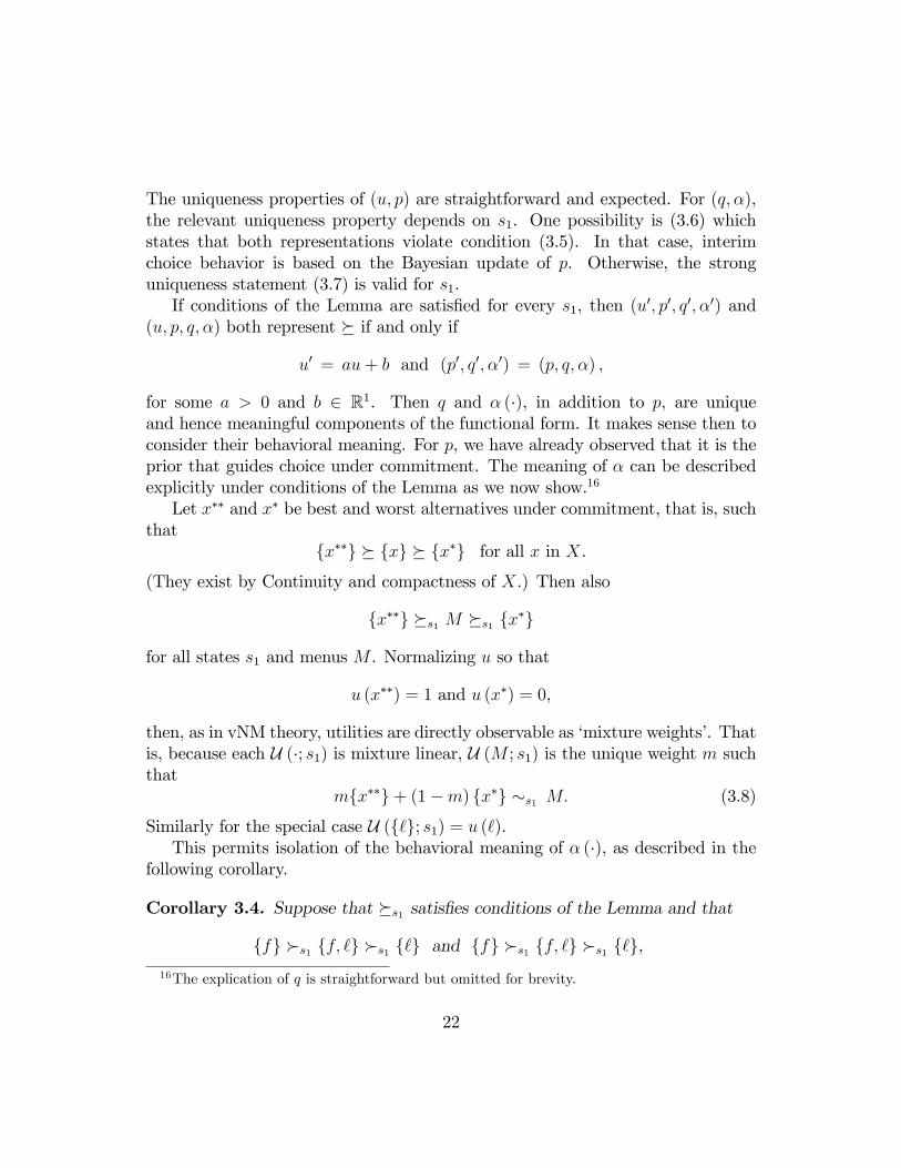
Corollary 3.4. Suppose that �s1 satis�es conditions of the Lemma and that

ffg �s1 ff; `g �s1 f`g and ffg �s1 ff; `g �s1 f`g,16The explication of q is straightforward but omitted for brevity.

22

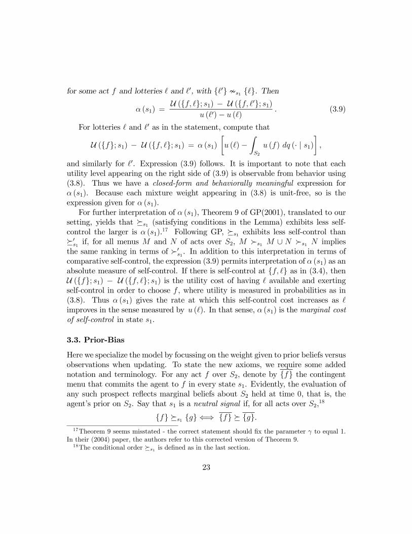
for some act f and lotteries ` and `0, with f`0g �s1 f`g. Then

� (s1) =U (ff; `g; s1) � U (ff; `0g; s1)

u (`0)� u (`) . (3.9)

For lotteries ` and `0 as in the statement, compute that

U (ffg; s1) � U (ff; `g; s1) = � (s1)

�u (`)�

ZS2

u (f) dq (� j s1)�,

and similarly for `0. Expression (3.9) follows. It is important to note that eachutility level appearing on the right side of (3.9) is observable from behavior using(3.8). Thus we have a closed-form and behaviorally meaningful expression for� (s1). Because each mixture weight appearing in (3.8) is unit-free, so is theexpression given for � (s1).For further interpretation of � (s1), Theorem 9 of GP(2001), translated to our

setting, yields that �s1 (satisfying conditions in the Lemma) exhibits less self-control the larger is � (s1).17 Following GP, �s1 exhibits less self-control than�0s1 if, for all menus M and N of acts over S2, M �s1 M [ N �s1 N impliesthe same ranking in terms of �0s1 . In addition to this interpretation in terms ofcomparative self-control, the expression (3.9) permits interpretation of � (s1) as anabsolute measure of self-control. If there is self-control at ff; `g as in (3.4), thenU (ffg; s1) � U (ff; `g; s1) is the utility cost of having ` available and exertingself-control in order to choose f , where utility is measured in probabilities as in(3.8). Thus � (s1) gives the rate at which this self-control cost increases as `improves in the sense measured by u (`). In that sense, � (s1) is the marginal costof self-control in state s1.

3.3. Prior-Bias

Here we specialize the model by focussing on the weight given to prior beliefs versusobservations when updating. To state the new axioms, we require some addednotation and terminology. For any act f over S2, denote by ffg the contingentmenu that commits the agent to f in every state s1. Evidently, the evaluation ofany such prospect re�ects marginal beliefs about S2 held at time 0, that is, theagent�s prior on S2. Say that s1 is a neutral signal if, for all acts over S2,18

ffg �s1 fgg () ffg � fgg.17Theorem 9 seems misstated - the correct statement should �x the parameter to equal 1.

In their (2004) paper, the authors refer to this corrected version of Theorem 9.18The conditional order �s1 is de�ned as in the last section.

23

Given our representation, s1 is a neutral signal if and only if p (� j s1) = p2 (�).

Axiom 9 (Prior-Bias). Let s1 2 S1 and let f and g be any acts over S2 satis-fying

ffg �s1 fgg.Then ffg �s1 ff; gg if either s1 is a neutral signal or if ffg � fgg.

To interpret, suppose that holding �xed what the contingent menu gives instates other than s1, committing to f in state s1 is strictly preferred to committingto g in state s1. By Set-Betweenness, ffg �s1 ff; gg, where strict preferenceindicates the expectation that g would be tempting in state s1, and hence thatupdating would lead to a change in beliefs from those currently held. Prior-Biasrules this out if s1 is a neutral signal. For any non-neutral s1, g can be temptinggiven s1 only if ffg � fgg, that is, only if prior beliefs di¤er on the two acts. Thatthe presence of temptation conditionally on s1 depends not only on how f and gare ranked conditionally but also on how attractive they were prior to realizationof s1, indicates excessive in�uence of prior beliefs at the updating stage.Prior-Bias permits prior beliefs to unduly in�uence updating but does not

specify the direction of such in�uence. Put another way, what happens if ffg andfgg are not indi¤erent? We consider two alternative strengthenings of the axiomthat provide di¤erent answers.

Axiom 10 (Positive Prior-Bias). Let s1 2 S1 and let f and g be any acts overS2 satisfying

ffg �s1 fgg.Then ffg �s1 ff; gg if either s1 is a neutral signal or if ffg � fgg.

According to this axiom, g can be tempting conditionally on a non-neutral s1only if it was strictly more attractive according to prior beliefs on S2. Intuitively,this is because prior beliefs are overweighted.An alternative strengthening of Prior-Bias is:

Axiom 11 (Negative Prior-Bias). Let s1 2 S1 and let f and g be any actsover S2 satisfying

ffg �s1 fgg.Then ffg �s1 ff; gg if either s1 is a neutral signal or if ffg � fgg.

24

Suppose that while g is (weakly) preferred according to prior beliefs on S2, the(necessarily non-neutral) signal s1 reverses the ranking in favor of f . The agentmodeled by this axiom overweights such a signal (and she knows this about herselfex ante). Thus she is not tempted by g after seeing s1 (or when anticipating itsrealization ex ante).

Corollary 3.5. Suppose that � satis�es the axioms in Theorem 3.1. Then �satis�es also Prior-Bias (Positive Prior-Bias or Negative Prior-Bias, respectively)if and only if it admits a representation (2.1)-(2.3) where in addition: for each s1,either � (s1) = 0, or � (s1) > 0 and

q (� j s1) = (1� � (s1)) p (� j s1) + � (s1) p2 (�) , (3.10)

with � (s1) � 1 (0 < � (s1) � 1, � (s1) � 0, respectively).

Prior-Bias leads to a concrete relation between the �temptation prior" q andthe commitment prior p: the Bayesian update of q is a linear combination ofthe Bayesian update of p and prior marginal beliefs p2 (�). As a result the agentdeviates from Bayesian updating by attaching a (positive or negative) additionalweight to prior beliefs over S2, where this additional weight is signed in the naturaldirection by Positive or Negative Prior-Bias. This functional form was interpretedfurther in Section 2.3. Note �nally that under Prior-Bias, q (� j s1) = p (� j s1) andupdating is standard if S1 is a singleton, or more generally, if p is a productmeasure.

4. CONCLUDING REMARKS

The connection of our model to updating relies on the interpretation of the func-tional form (2.5) as describing interim choice at time 1. This interpretation issuggested by our formal model, but Theorem 3.1 deals only with the ex antechoice between contingent menus and not with the interim choice of acts frommenus. A similar issue arises in the GP model and their solution, using suitablyextended preferences, can be adapted here. Note that foundations provided inthis way are subject to the di¢ culty pointed out in GP (2001, p. 1415), namelythe lack of a revealed preference basis for extended preferences.One might expect a given individual to update di¤erently in di¤erent situa-

tions. If by �situation�one means �state space�, then the present model is consis-tent with such variation because it is restricted to a given state space. However,

25

it has nothing to say about how behavior is connected across state spaces. Al-ternatively, one might expect that even given the state space, an individual mayexhibit di¤erent updating biases depending on the choice problem. This calls fora generalization that would permit updating behavior to depend on the menuavailable at the interim stage.Conclude with one application of the model. Our non-Bayesian agent violates

the law of iterated expectations, because she uses the compromise measure p�

from (2.6) to guide choice at t = 1 but she uses p for choice at t = 0. Thus thereexist acts f : S2 �! X such that ffg � f�fg at time 0 and yet such that at eachs1, the agent would strictly prefer to choose �f out of ff;�fg. This amounts toa violation of the �sure-thing principle for action rules�, a property that has beenidenti�ed as central to no-trade theorems, (see Geanakoplos (1994), for example).It is not surprising, therefore, that two such agents may agree to take oppositesides of a bet at every state s1 even if they have common commitment priors andall the preceding is common knowledge. What may be not so obvious, however,is that common knowledge agreement to bet can arise even though agents havestable (unchanging) preferences, albeit over contingent menus rather than on theusual domain of acts. Future research will explore more deeply the message ofthis example - that trade may result not only from heterogeneity in prior beliefsor in information, but also from heterogeneity in the way that agents update inresponse to information.

A. APPENDIX: Proofs of Main Results

Proof of Theorem 3.1: Necessity: Set-Betweenness is satis�ed because each U (�; s1)de�ned in (2.3) has the GP form. Verify State Independence; veri�cation of theother axioms is immediate.Claim 1: p (s1; s2) > 0 =) (s1; s2) is non-null. Take any F with F (s1) = Ls2Mand de�ne F 0 by

F 0 (s01) = F (s01) if s

01 6= s1 and F 0 (s1) = L0s2M .

Compute that U (Ls2M ; s1) =

maxf2Ls2M

�ZS2

u (f) dp(� j s1) + � (s1)

ZS2

u (f) dq(� j s1)�

� maxf 02Ls2M

� (s1)

ZS2

u (f 0) dq(� j s1)

26

= maxf2M

�ZS2nfs2g

u (f) dp(� j s1) + � (s1)

ZS2nfs2g

u (f) dq(� j s1)�

� maxf 02M

� (s1)

ZS2nfs2g

u (f 0) dq(� j s1)

+ max`2L

fu (`) p(s2 j s1) + � (s1) u (`) q(s2 j s1)g �max`02L

� (s1)u (`0) q(s2 j s1).

It follows that

U (F 0)� U (F ) = p1 (s1)�p(s2 j s1) max

`2L0u (`)� p(s2 j s1) max

`2Lu (`)

�

= p (s1; s2)

�max`2L0

u (`)�max`2L

u (`)

�.

Because u (�) is not constant, we can choose L0 and L so that the latter expressionis nonzero. This proves that (s1; s2) is non-null.

Claim 2: p (s1; s2) = 0 =) (s1; s2) is null. Compute that U (F (s1) ; s1) =

maxf2F (s1)

�ZS2

u (f) dp(� j s1) + � (s1)

ZS2

u (f) dq(� j s1)�

� maxf 02F (s1)

� (s1)

ZS2

u (f 0) dq(� j s1).

Because q << p, the right hand side does not depend on ff (s2) : f 2 F (s1)g. Inother words, �

f 0�s2 : f0 2 F 0 (s1)

= ff�s2 : f : f 2 F (s1)g =)

U (F 0 (s1) ; s1) = U (F (s1) ; s1) .It follows that (s1; s2) is null.

Return to State Independence. For any menus of lotteries,

L0 � L() max`2L0

u (`) � max`2L

u (`) :

Also, U (F�s1 ; L0s2F (s1))� U (F�s1 ; Ls2F (s1)) = p (s1; s2) [max`2L0 u (`)�max`2L u (`)],by the calculations above. Thus State Independence follows from the precedingclaims.

27

Su¢ ciency: We claim that because � satis�es Order, Continuity and Indepen-dence on C, there exists a representation for � of the form

U (F ) = �s12S1 U (F (s1) ; s1) , (A.1)

where each U (�; s1) is continuous and mixture linear on M (S2). Intuition forthis claim is provided by the similarity with the Anscombe-Aumann theorem.The latter deals with acts mapping a state space into �(X), while here eachF maps states into M (S2), which shares with �(X) the existence of a mixingoperation. However, M (S2) is not a mixture space and thus the analogy is notperfect.19 To �ll this gap, denote by coF the contingent menu taking s1 intothe closed convex hull of F (s1). The vNM axioms imply that coF and F areindi¤erent (see Lemma 1 in Dekel, Lipman and Rustichini (2001)). Moreover, thesubdomain ofM (S2) consisting of closed and convex menus is a mixture space,and thus standard arguments apply to deliver the desired representation there.Finally, extend the representation using the noted indi¤erence between coF andF .It follows that for each s1, � induces the conditional order �s1 onM (S2) via

M 0 �s1 M if (F�s1 ;M0) � (F�s1 ;M) for some F ,

and that �s1 is represented by U (�; s1). By Set-Betweenness, �s1 satis�es the GPaxioms suitably translated to our setting; that is, GP deal with menus of lotteries,while we have menus of Anscombe-Aumann acts over S2. With this translation,their proof is valid for our setting and delivers:20

U (M ; s1) = maxf2M

�U (f ; s1) + V (f ; s1)�max

f 02MV (f 0; s1)

�, (A.2)

where U (�; s1) and V (�; s1) are mixture linear (and continuous). Actually, thepreceding equality is valid only up to ordinal equivalence, but both sides aremixture linear and so they must be cardinally equivalent. Thus absolute equalitymay be assumed wlog.Both U (�; s1) and V (�; s1), utility functions de�ned on the domain (� (X))S2

of Anscombe-Aumann acts, satisfy the basic mixture space axioms there. Thus,by Kreps (1988, Propn. 7.4) and Continuity, we can write

U (f ; s1) = �s22S2 u (f (s2) ; s1; s2) , V (f ; s1) = �s22S2 v (f (s2) ; s1; s2) , (A.3)

19It violates the property ���0M +

�1� �0

�N�+ (1� �) N = ��0M +

�1� ��0

�N .

20In fact, Kopylov (2005) has extended the GP theorem to a domain of menus of any compactmetric mixture space where the mixture operation is continuous.

28

for all f : S2 �! �(X). (Below we often abbreviate (s1; s2) by s.) Each u (�; s)and v (�; s) is mixture linear and continuous.

Lemma A.1. Assume Order, State Independence and Nondegeneracy. Then:(a) For all (s1; s2) and non-null (s01; s

02), contingent menus F , menus M of acts

over S2 and menus L0 and L of lotteries,

L0s02M �s01 Ls02M =) L0s2M �s1 Ls2M .

(b) For all (s1; s2) and contingent menus F , if

L0s2F (s1) �s1 Ls2F (s1)

for all menus of lotteries L0 and L, then (s1; s2) is null.

Proof. (a) Since (s01; s02) is non-null, State Independence applied twice implies

L0s02M �s01 Ls02M =) L0 � L =) L0s2M �s1 Ls2M .

(b) Under the stated hypothesis, if (s1; s2) were non-null, then Order and StateIndependence would imply L0 � L for all L0 and L, contradicting Nondegeneracy.Therefore, (s1; s2) is null.

Take F 2 A, that is, let F (s1) be a singleton for every s1. Recall that A isisomorphic to (� (X))S1�S2, the set of Anscombe-Aumann acts over S1�S2. Thepreceding three displayed equations imply that � restricted to A is representedby bU , where

bU � bf� = �s1;s2 u� bf (s1; s2) ; s1; s2� , for all bf 2 (� (X))S1�S2 .

By part (a) of the Lemma and Nondegeneracy, the order represented by bU (�)satis�es all the Anscombe-Aumann axioms. Thus (by Kreps (1988, Theorem7.17), for example) bU has the SEU form

bU � bf� = �s2S1�S2 p (s) u� bf (s)� ,

for a suitable nonconstant and mixture linear u and probability measure p onS1 � S2. (Equality is modulo ordinal equivalence, but the latter quali�cation can

29

be dropped because bU (�) is mixture linear, forcing the ordinal transformation tobe cardinal.) Wlog therefore,

u (�; s1; s2) = p (s1; s2) u (�)

and we can re�ne (A.3) and write

U (f ; s1) = �s22S2 p (s1; s2) u (f (s2)) . (A.4)

The next step is to show that on X,

v (�; s) = asp (s)u (�) + bs, where as � 0. (A.5)

To do so, note that for any s = (s1; s2) and menus M 2 M (S2) and L0; L ��(X),

L0s2M �s1 Ls2M () U (L0s2M ; s1) � U (Ls2M ; s1) ,where

U (Ls2M ; s1) = maxf2M; `2L

fU (`s2f ; s1) + V (`s2f ; s1)g

� maxf 02M; `02L

V (`0s2f0; s1) , and hence

U (Ls2M ; s1) = max`2L

�p (s) u (`) + v (`; s) �max

`02Lv (`0; s)

�+ �(M; s) , (A.6)

where the �nal term is independent of L and can be ignored for present purposes.We claim that the ranking of menus of lotteries represented by L 7�! U (Ls2M ; s1),

or equivalently by

L 7�! max`2L

�p (s) u (`) + v (`; s) �max

`02Lv (`0; s)

�,

is strategically rational, that is,

L0s2M �s1 Ls2M =) L0s2M �s1 (L0 [ L) s2M .

The indi¤erence on the RHS is trivially true if (s1; s2) is null. Otherwise, the im-plication follows from State Independence and Strategic Rationality for Lotteries.

Case 1: Suppose p (s) > 0. Then p (s)u (�) is nonconstant. Hence (A.5) follows asin GP(2001, p. 1414) from the just noted strategic rationality.

30

Case 2: Suppose that p (s) = 0. Then by part (b) of the Lemma, s = (s1; s2) isnull, and by the de�nition of nullity, the utility of any F is independent of whatit assigns to the state s. Thus any speci�cation for v(�; s) is consistent with arepresentation for �. In particular, we can take v (�; s) = 0 wlog and (A.5) is validwith as = 0.

From (A.3)-(A.5), deduce that

U (M ; s1) = maxf2M

f�s2 p (s1; s2)u (f (s2)) + �s2as1;s2p (s1; s2)u (f (s2))g

�maxf 02M

f�s2as1;s2p (s1; s2)u (f 0 (s2))g .

Denote by p1 the S1-marginal of p; it is everywhere positive by (A.3), (A.5) andS1-Full Support. Let

� (s1) =�s2as1;s2p (s1; s2)

p1 (s1),

and de�ne the measure q so that its S1-marginal equals p1, and

q (s2 j s1) =(

as1;s2p(s2js1)�(s1)

if � (s1) > 0p (s2 j s1) otherwise.

Then

U (M ; s1) = p1 (s1) maxf2M

f�s2 p (s2 j s1)u (f (s2)) + � (s1) �s2q (s2 j s1)u (f (s2))g

�p1 (s1) maxf 02M

f� (s1) �s2q (s2 j s1)u (f 0 (s2))g .

With (A.1), this yields the desired representation (2.1)-(2.2).

Proof of Corollary 3.3: If (u; p; q; �) represents � and if (u0; p0; q0; �0) is related asstated, then clearly it also represents�. For the converse, suppose that both tuplesrepresent �. Then the subjective expected utility functions de�ned by (u; p) and(u0; p0) both represent preference on the subset A � C of Anscombe-Aumann actsover S1�S2. By the well-known uniqueness properties of the Anscombe-Aumanntheorem,

u0 = au+ b and p0 = p: (A.7)

31

By Lemma 3.2, (u0; p0; q0; �0) violates (3.5) i¤ (u; p; q; �) does, in which case(3.6) is valid. Suppose that (u; p; q; �) satis�es (3.5). The latter implies thatU (�; s1) is regular in the sense of GP (2001, p. 1414). (Here and below we refer tothe translation of GP to our setup, whereby their menus of lotteries are replacedby menus of Anscombe-Aumann acts over S2.) Thus their Theorem 4 implies that

V 0 (�; s1) = As1V (�; s1) + BV; s1 and (A.8)

U 0 (�; s1) = As1U (�; s1) + BU; s1, (A.9)

where

V (f ; s1) = � (s1)

ZS2

u (f) dq(� j s1), f 2 (� (X))S2 , (A.10)

and V 0; U 0; V and U are de�ned similarly. Deduce from (A.7) and (A.9) thatAs1 = a. Equation (A.8) implies, again by uniqueness properties of the Anscombe-Aumann model, that q0 (� j s1) = q (� j s1). Substitution from (A.10) implies fur-ther that

�0 (s1)

ZS2

(au (f) + b) dq(� j s1) = a� (s1)ZS2

u (f) dq(� j s1) + BV; s1,

for all f 2 (� (X))S2, which implies that �0 (s1) = � (s1).

Proof of Corollary 3.5: The necessity assertions are obvious. Prove su¢ ciency ofPrior-Bias; the arguments for Positive and Negative Prior-Bias are similar. Givenour representation, if � (s1) > 0, then Prior-Bias implies:

ifZ(u (f)� u (g)) dp (� j s1) > 0 and

Z(u (f)� u (g)) dp2 (�) = 0,

thenZ(u (f)� u (g)) dq (� j s1) � 0.

By Motzkin�s Theorem of the Alternative (see Mangasarian (1969, p. 34),

ypp (� j s1)� yqq (� j s1) + y2p2 (�) = 0 (A.11)

for some scalars yp � 0; yq � 0 and y2, with yp + yq > 0.

32

Case 1 (yq > 0): Solve (A.11) for q (� j s1) and deduce (3.10).Case 2 (yq = 0): Then necessarily p (� j s1) = p2 (�). Thus s1 is a neutral signaland Prior-Bias implies that ffg �s1 ff; gg. In fact, the corresponding indi¤erenceholds for any pair of acts f 0 and g0 for which ff 0g �s1 fg0g, that is,Z

(u (f 0)� u (g0)) dp (� j s1) > 0 =)Z(u (f 0)� u (g0)) dq (� j s1) � 0.

Conclude that q (� j s1) = p (� j s1).

B. APPENDIX: Changing Risk Aversion

This appendix elaborates on the model of changing risk preference mentioned inSection 2.2. More precisely, consider the utility function on C given by

U (F ) =ZS1

U (F (s1) ; s1) dp1, F 2 C, (B.1)

and U (F (s1) ; s1) =�maxf2F (s1)

ZS2

[u (f) + v (f)] dp(� j s1)�� max

f 02F (s1)

ZS2

v (f 0) dp(� j s1), (B.2)

where:

Reg1* u; v : � (X) �! R1 are mixture linear and continuous.

Reg2* each p (� j s1) is a probability measure on S2.

Reg3* There exist lotteries `0 and ` such that v (`0) < v (`) and u (`0) + v (`0) >u (`) + v (`).

Reg4* u cannot be expressed as the linear transformation u = av+ b, where a < 0.

Note that these conditions rule out the standard Bayesian model (say if v isconstant or a positive a¢ ne transformation of u) and that the above model isdisjoint from our central model. Turn to the axioms that underlie them.Adopt all previous axioms with the exception of Strategic Rationality for Lot-

teries (SRL). To state its replacement, adapt terminology from GP. Say that� has

33

self-control for lotteries if L0 � L0 [ L � L for some menus of lotteries. Considernext:21

Axiom 12 (Regular Self-Control for Lotteries (RSCL)). � has self-controlfor lotteries and there exists L such that: (i) L � L00 for all subsets L00 of L, and(ii) L � f`g for some ` in L.

To interpret the axiom, compare it with SRL. The latter says that where thechoice is between (unconditional) menus of lotteries, then there is no temptation,while the new axiom says the opposite - that temptation sometimes occurs evenfor such choices. Thus while SRL implies that temptation arises only where beliefsare relevant for choice, RSCL implies that it arises even where only risk attitudeis relevant for choice. This explains why substituting RSCL for SRL leads to thefollowing alternative to Theorem 3.1.

Theorem B.1. � satis�es Order, Continuity, Independence, Nondegeneracy, Set-Betweenness, Regular Self-Control for Lotteries, State Independence and S1-FullSupport if and only if it admits a representation of the form (B.1)-(B.2), includingthe regularity conditions Reg1*-Reg4*.

Though Theorems 3.1 and B.1 are disjoint, they do not exhaust the class ofpreferences satisfying all their common axioms. As an example, take (B.1) andU (F (s1) ; s1) =�maxf2F (s1)

ZS2

u (f) dp(� j s1)� �ZS2

u (f) dq(� j s1)�� maxf 02F (s1)

(��)ZS2

u (f) dq(� j s1)

=

�maxf2F (s1)

ZS2

u (f) dp(� j s1)� �ZS2

u (f) dq(� j s1)�+ minf 02F (s1)

�

ZS2

u (f) dq(� j s1),

where q(� j s1) << p(� j s1) and 1 < �. Though all other axioms are satis�ed,SRL and RSCL are violated and thus the functional form does not �t into eithermodel. The interpretation is that the underlying �change in preference�cannotbe attributed to a change in only one of taste or beliefs.22

21GP (2001, p. 1414) refer to (i)-(ii) as the absence of maximal preference for commitment.They also de�ne regularity. The connection is that, given that � has self-control, then � hasregular self-control i¤ it is regular.22The obvious funtional form based on arbitrary pairs (u; p) and (v; q) would also support

such a statement, but it would violate State Independence.

34

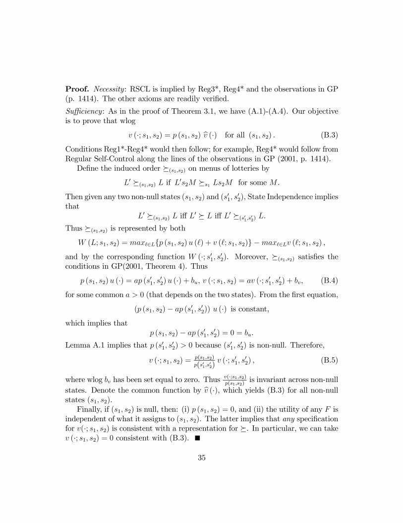
Proof. Necessity: RSCL is implied by Reg3*, Reg4* and the observations in GP(p. 1414). The other axioms are readily veri�ed.

Su¢ ciency: As in the proof of Theorem 3.1, we have (A.1)-(A.4). Our objectiveis to prove that wlog

v (�; s1; s2) = p (s1; s2) bv (�) for all (s1; s2) . (B.3)

Conditions Reg1*-Reg4* would then follow; for example, Reg4* would follow fromRegular Self-Control along the lines of the observations in GP (2001, p. 1414).De�ne the induced order �(s1;s2) on menus of lotteries by

L0 �(s1;s2) L if L0s2M �s1 Ls2M for some M .

Then given any two non-null states (s1; s2) and (s01; s02), State Independence implies

thatL0 �(s1;s2) L i¤ L0 � L i¤ L0 �(s01;s02) L.

Thus �(s1;s2) is represented by both

W (L; s1; s2) = max`2Lfp (s1; s2)u (`) + v (`; s1; s2)g �max`2Lv (`; s1; s2) ,

and by the corresponding function W (�; s01; s02). Moreover, �(s1;s2) satis�es theconditions in GP(2001, Theorem 4). Thus

p (s1; s2)u (�) = ap (s01; s02)u (�) + bu, v (�; s1; s2) = av (�; s01; s02) + bv, (B.4)

for some common a > 0 (that depends on the two states). From the �rst equation,

(p (s1; s2)� ap (s01; s02)) u (�) is constant,

which implies thatp (s1; s2)� ap (s01; s02) = 0 = bu.

Lemma A.1 implies that p (s01; s02) > 0 because (s

01; s

02) is non-null. Therefore,

v (�; s1; s2) = p(s1;s2)

p(s01;s02)v (�; s01; s02) , (B.5)

where wlog bv has been set equal to zero. Thusv(�;s1;s2)p(s1;s2)

is invariant across non-nullstates. Denote the common function by bv (�), which yields (B.3) for all non-nullstates (s1; s2).Finally, if (s1; s2) is null, then: (i) p (s1; s2) = 0, and (ii) the utility of any F is

independent of what it assigns to (s1; s2). The latter implies that any speci�cationfor v(�; s1; s2) is consistent with a representation for �. In particular, we can takev (�; s1; s2) = 0 consistent with (B.3).

35

References

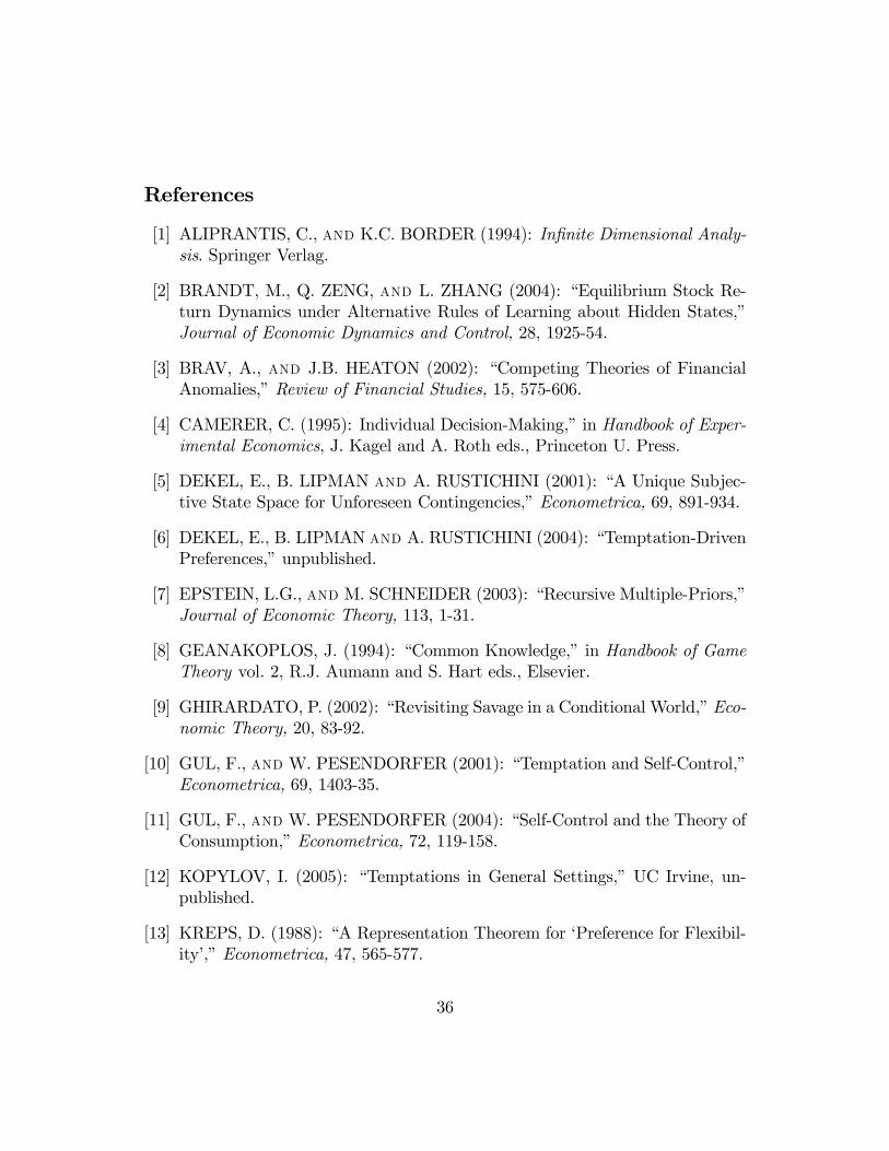
[1] ALIPRANTIS, C., and K.C. BORDER (1994): In�nite Dimensional Analy-sis. Springer Verlag.

[2] BRANDT, M., Q. ZENG, and L. ZHANG (2004): �Equilibrium Stock Re-turn Dynamics under Alternative Rules of Learning about Hidden States,�Journal of Economic Dynamics and Control, 28, 1925-54.

[3] BRAV, A., and J.B. HEATON (2002): �Competing Theories of FinancialAnomalies,�Review of Financial Studies, 15, 575-606.

[4] CAMERER, C. (1995): Individual Decision-Making,�in Handbook of Exper-imental Economics, J. Kagel and A. Roth eds., Princeton U. Press.

[5] DEKEL, E., B. LIPMAN and A. RUSTICHINI (2001): �A Unique Subjec-tive State Space for Unforeseen Contingencies,�Econometrica, 69, 891-934.

[6] DEKEL, E., B. LIPMAN and A. RUSTICHINI (2004): �Temptation-DrivenPreferences,�unpublished.

[7] EPSTEIN, L.G., and M. SCHNEIDER (2003): �Recursive Multiple-Priors,�Journal of Economic Theory, 113, 1-31.

[8] GEANAKOPLOS, J. (1994): �Common Knowledge,�in Handbook of GameTheory vol. 2, R.J. Aumann and S. Hart eds., Elsevier.

[9] GHIRARDATO, P. (2002): �Revisiting Savage in a Conditional World,�Eco-nomic Theory, 20, 83-92.

[10] GUL, F., andW. PESENDORFER (2001): �Temptation and Self-Control,�Econometrica, 69, 1403-35.

[11] GUL, F., andW. PESENDORFER (2004): �Self-Control and the Theory ofConsumption,�Econometrica, 72, 119-158.

[12] KOPYLOV, I. (2005): �Temptations in General Settings,�UC Irvine, un-published.

[13] KREPS, D. (1988): �A Representation Theorem for �Preference for Flexibil-ity�,�Econometrica, 47, 565-577.

36

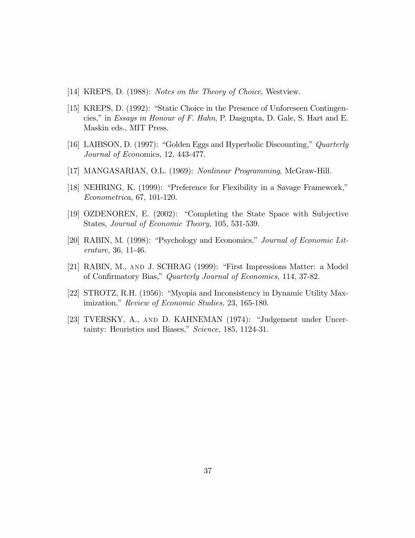
[14] KREPS, D. (1988): Notes on the Theory of Choice, Westview.

[15] KREPS, D. (1992): �Static Choice in the Presence of Unforeseen Contingen-cies,�in Essays in Honour of F. Hahn, P. Dasgupta, D. Gale, S. Hart and E.Maskin eds., MIT Press.

[16] LAIBSON, D. (1997): �Golden Eggs and Hyperbolic Discounting,�QuarterlyJournal of Economics, 12, 443-477.

[17] MANGASARIAN, O.L. (1969): Nonlinear Programming, McGraw-Hill.

[18] NEHRING, K. (1999): �Preference for Flexibility in a Savage Framework,�Econometrica, 67, 101-120.

[19] OZDENOREN, E. (2002): �Completing the State Space with SubjectiveStates, Journal of Economic Theory, 105, 531-539.

[20] RABIN, M. (1998): �Psychology and Economics,�Journal of Economic Lit-erature, 36, 11-46.

[21] RABIN, M., and J. SCHRAG (1999): �First Impressions Matter: a Modelof Con�rmatory Bias,�Quarterly Journal of Economics, 114, 37-82.

[22] STROTZ, R.H. (1956): �Myopia and Inconsistency in Dynamic Utility Max-imization,�Review of Economic Studies, 23, 165-180.

[23] TVERSKY, A., and D. KAHNEMAN (1974): �Judgement under Uncer-tainty: Heuristics and Biases,�Science, 185, 1124-31.

37