Embed Size (px)
Citation preview

An Autonomous Navigation Systemfor Lunar and Planetary Exploration Rovers
Douglas Hemingway
Individual Project Report submitted to the International Space University in partial
fulfillment of the requirements of the M.Sc. Degree in Space Studies
August, 2009
Internship Mentor: Dr. Takashi KUBOTA
Host Institution: Japan Aerospace Exploration Agency
Institute of Space and Astronautical Science
Sagamihara, Japan
ISU Academic Advisor: Dr. Yoshiki MORINO

ii
Acknowledgements
First, I would like to thank the European Space Agency whose generous financial support enabled me
to participate in the ISU Masters program this year.
I would also like to thank the ISU faculty and staff in Strasbourg, especially my academic advisor
Dr.!Yoshiki!Morino for his support in helping me secure an internship in Japan.
At the Japan Aerospace Exploration Agency (JAXA) Institute of Space and Astronautical Sciences
(ISAS) in Sagamihara, Japan, I would like to thank my advisor, Dr. Takashi Kubota for hosting me in
his robotics lab this summer.
Finally, I would like to thank my distinguished colleague, Kevin Frugier, whose lent expertise in
OpenGL was an asset to my project.
iii
Abstract
Surface exploration of solar system bodies is one of the most crucial tools available to
researchers wishing to learn about the history of the solar system and the rise of life within it.
Mobile robots are, and will continue to be, the major workhorse of solar system exploration,
reaching places where humans cannot go and supporting human crews where they can. The
productivity of these robots is largely a function of their ability to make their own decisions,
minimizing time spent waiting for instructions from Earth-based mission controllers. The
most basic level of autonomy that is required is the capability to identify and circumnavigate
obstacles.
The work presented here focuses on the ISAS (Institute of Space and Astronautical Science)
M6 rover as a platform for the development of an autonomous navigation system. The goal
has been to implement a basic working system that will serve as a starting point for
researchers developing autonomous navigation system components. It is hoped that the
modular approach of the implementation will allow researchers to replace or modify
individual components in an otherwise working framework. This will allow new ideas and
algorithms to be tested directly in field trials, helping the ideas to mature more rapidly and
with greater confidence. The main sources of sensor input for the system are stereo vision
and LIDAR (Light Detection and Ranging). Since little work had so far been done with
LIDAR, this was chosen as the sole input source for the prototype implementation, serving a
secondary project goal of verifying the effectiveness of using LIDAR as a primary input.
The annual ISAS Open House, held this year on July 25, was chosen as a target date for
completion of a prototype implementation. By this date, the system was able to complete a
scan of the area in front of the robot, build a world model from the laser measurements, assess
the traversability of the terrain, and finally plan an obstacle-avoiding path to a specified
destination using a simple custom-made path planning algorithm. While the results have been
generally satisfactory, this implementation is meant only to be a starting point. It is expected
that the system will be improved and augmented over time, gradually increasing robustness
and autonomy, progressing toward an ever more capable and productive rover for lunar and
planetary exploration.
iv
Table of Contents
Acknowledgements .................................................................................................... ii
Abstract ..................................................................................................................... iii
1 Introduction ..........................................................................................................11.1 Robotics in Solar System Exploration......................................................................1
1.2 Autonomy in Mobile Robotics..................................................................................21.2.1 The Need for Autonomy...................................................................................................21.2.2 Approaches for Increased Autonomy..............................................................................3
1.3 Project Context and Objectives ...............................................................................51.3.1 Rover Technology in Japan.............................................................................................51.3.2 Stereo Vision and LIDAR for Navigation.........................................................................71.3.3 Scope and Objectives......................................................................................................7
2 System Concepts .................................................................................................92.1 Operations Concept................................................................................................9
2.1.1 Behaviour Layers .............................................................................................................92.1.2 M6 Rover Operations.....................................................................................................11
2.2 Problem Definition ................................................................................................13
2.3 Assumptions.........................................................................................................132.3.1 Sensing...........................................................................................................................132.3.2 Modelling and Mapping..................................................................................................142.3.3 Terrain Assessment and Costing ..................................................................................152.3.4 Path Planning.................................................................................................................162.3.5 Directing the Rover ........................................................................................................172.3.6 Summary of Key Assumptions ......................................................................................17
2.4 Navigation System Overview ................................................................................18
3 Implementation...................................................................................................193.1 Sensing ................................................................................................................19
3.1.1 Laser Range Finder and Its Data ..................................................................................193.1.2 Noise and Filtering .........................................................................................................22
3.2 Modelling and Mapping.........................................................................................253.2.1 Transforming the Sensor Data into Cartesian Space...................................................253.2.2 Cartesian Space Point Cloud ........................................................................................273.2.3 Model Format Options ...................................................................................................283.2.4 Digital Elevation Model (DEM) Prototype Implementation...........................................29
3.3 Terrain Assessment and Costing ..........................................................................313.3.1 Potential Approaches.....................................................................................................313.3.2 Solution for the Prototype Implementation....................................................................31
3.4 Path Planning.......................................................................................................323.4.1 Potential Approaches.....................................................................................................333.4.2 Solution for the Prototype Implementation....................................................................34
3.5 Communications and Operating Modes ................................................................39

v
4 Discussion and Future Work ..............................................................................414.1 Experimental Results............................................................................................41
4.1.1 Laser Range Finder (LRF) Results ...............................................................................414.1.2 Modelling Results...........................................................................................................424.1.3 Costing Results ..............................................................................................................434.1.4 Path Planning Results....................................................................................................454.1.5 Open House Demonstrations ........................................................................................46
4.2 Proposed System Improvements ..........................................................................504.2.1 Programming Language ................................................................................................504.2.2 Terrain Assessment and Costing ..................................................................................504.2.3 Point Tracking for Localization ......................................................................................514.2.4 Path Planning.................................................................................................................524.2.5 Stereo Vision ..................................................................................................................52
4.3 System Expansion................................................................................................52
5 Conclusions........................................................................................................54
References ...............................................................................................................56
Glossary ...................................................................................................................58
vi
List of Figures
Figure 1.1: Micro-5 Rover (Kuroda et al., 1999) .................................................................... 5
Figure 1.2: Fleet of M6 Rovers .............................................................................................. 6
Figure 2.1: 3-Layer Architecture for Robot Autonomy ........................................................ 10
Figure 2.2: Existing Implementation.................................................................................... 11
Figure 2.3: Navigation System Testing Implementation....................................................... 12
Figure 2.4: Standard Aircraft Coordinate Frame Convention ............................................... 14
Figure 2.5: ISAS M6 Rover Frame Convention ................................................................... 14
Figure 2.6: Navigation System Overview............................................................................. 18
Figure 3.1: Nippon Signal Laser Range Finder .................................................................... 19
Figure 3.2: Rotating Mirror inside LRF ............................................................................... 20
Figure 3.3: Depth and Reflectivity Measured by LIDAR ..................................................... 21
Figure 3.4: Photograph of the Scanned Scene ...................................................................... 21
Figure 3.5: Non-credible Data Points in Raw LRF Data....................................................... 22
Figure 3.6: Inadequacy of Simplistic Filters......................................................................... 23
Figure 3.7: Data Points Before and After Filter Appliation .................................................. 24
Figure 3.8: Depth Map Filtering .......................................................................................... 24
Figure 3.9: Arbitrary Point, P, Relative to the Sensor........................................................... 25
Figure 3.10: Aribtrary Point, P, as Seen in the Depth Map Image......................................... 25
Figure 3.11: View Perpendicular to Vertical Plane Containing d.......................................... 26
Figure 3.12: Overhead View Showing d Projected Onto X-Y Plane as d cos!...................... 26
Figure 3.13: Point Cloud in a Cartesian Grid ....................................................................... 27
Figure 3.14: Terrain Model of Candor Chasma, Mars (GoogleEarth, 2009) ......................... 29
Figure 3.15: Accumulation of Multiple Scans Into Single DEM........................................... 30
Figure 3.16: Point Cloud with Data Points Clustered on Obstacles....................................... 32
Figure 3.17: Initially-Assumed Path is Already Clear .......................................................... 35
Figure 3.18: Initially-Assumed Path is Not Clear ................................................................. 35
Figure 3.19: Algorithm Encounters an Obstacle and Steps to the Side.................................. 36
Figure 3.20: Waypoint Inserted to the Side of the Obstacle .................................................. 36
Figure 3.21: New Collision Created..................................................................................... 37
Figure 3.22: Another Waypoint is Inserted .......................................................................... 37
Figure 3.23: Final Path is Clear of All Obstacles.................................................................. 38
Figure 3.24: Path Planning Algorithm Result Before Simplification .................................... 38
Figure 3.25: Path Planning Algorithm Result After Simplification....................................... 39
Figure 4.1: Detection of Rocks as Obstacles ........................................................................ 44
Figure 4.2: ISAS M6 Rover at Open House, July 25, 2009 .................................................. 46
Figure 4.3: ISAS M6 Rover Approaching Spectators at the Open House Demonstrations .... 47
Figure 4.4: LIDAR Scan of Spectators at the Edge of the Demonstration Field.................... 48
Figure 4.5: 3D DEM Modelling Spectators with Vertical Columns...................................... 48
Figure 4.6: 2D and 3D DEM Identifying Obstacles (shown in red) ...................................... 49
Figure 4.7: Obstacle-Avoiding Path Planned Around Spectators .......................................... 49
1
1 Introduction
Physical exploration of the solar system has been underway for several decades now.
Beginning with Luna 1 in 1959, the first human-made object to leave the vicinity of the Earth
(Harvey, 2008), humans have moved from Earth-based observation as the only means of
learning about the solar system, to direct physical exploration. To date, the Apollo program
of 1969-1971 remains the only example of human beings exploring the surfaces of other
worlds. In the coming decades, human crews are expected to return to the Moon to resume
the effort of human exploration. This will lay the groundwork for exploration of other solar
system bodies such as asteroids, the planet Mars, and more. Meanwhile, the major workhorse
of planetary exploration has been, and will continue to be, robots. Even as human exploration
activity increases, there will be an ongoing need for robotics in: 1) exploring bodies that are
too distant or too hostile for human missions; and 2) cooperatively supporting human crews
during surface operations.
1.1 Robotics in Solar System Exploration
When it landed on the Moon in 1966, Luna 9 became the first spacecraft to achieve a soft
landing on anther solar system body (Harvey, 2008). This marked the beginning of on-
surface data gathering from other worlds. Since then, robotic surface explorers have
blossomed in complexity through the stationary Surveyor, Venera/Vega, Viking, and ‘Mars’
lander programs to the first mobile surface explorers, Lunokhod, Mars Pathfinder’s
Sojourner, and most recently, the overwhelmingly successful twin Mars Exploration Rovers
(MERs), Spirit and Opportunity.
The advantage of mobility cannot be overstated. Most obviously, mobility extends surface
exploration from a few square meters of coverage at best, to several orders of magnitude
greater coverage, if not more. Exploration of the Martian surface, previously limited to the
immediate vicinity of a handful of landers, has now been vastly expanded by the recent and
ongoing MER mission whose rovers, Spirit and Opportunity, have so far traversed over 7.7
km and 17 km, respectively (Viotti, 2009). Mobility also allows for the possibility of
studying regions that are unsuitable as landing sites. Clearly, scientific yield is dramatically
increased when an exploration mission has mobility and thus the capability of investigating a
wider range of surface features in a variety of locations.
As exploration efforts continue, mobile robotic explorers will continue to be sent to study
lunar and planetary surfaces throughout the solar system. Initially, their role will be to
provide scientists with the first glimpses of alien world surfaces, the first geochemical
analyses of soil and rock samples, and the first opportunities to actively search for evidence of
water and ultimately indications of life whether extinct or extant.
In the fullness of time – and this may mean centuries of steady technological development –
many if not most solid bodies in the solar system should become accessible to human
explorers. For quite some time yet, however, robotic explorers may be the only practical
means for on-surface study of most of the solar system bodies. Since each body is another
clue to the history of the solar system and the life that arose within it, the development of
technology for productive, mobile robotic surface exploration is essential.
2
Apart from scientific study, mobile robots will also play a crucial role in scouting planetary
surfaces in preparation for future human exploration missions. The first task of the scouts
will likely be to evaluate the suitability of sites for human crews. Characterization of the soil
stability, for example, may be necessary prior to beginning construction of an outpost. To the
greatest practical extent, robots will also be used to begin building the infrastructure for such
outposts prior to the arrival of human crews. This helps ensure that crews have the best
possible start when they arrive and minimizes the risk that a failure of part of the outpost
construction process will have a critical impact on the mission.
Finally, once human crews do arrive, robotics will have a continuing role in assisting these
crews in their surface activities. Handling of very massive or cumbersome payloads or rock
and soil, will require the assistance of robotic cranes and vehicles. Activities requiring more
time than crews are able to dedicate in a single EVA (Extra-Vehicular Activity) will require
robots instead. For tasks requiring a combination of human flexibility and ingenuity along
with robotic strength and endurance, surface crews will work extensively in cooperation with
mobile robotic assistants.
1.2 Autonomy in Mobile Robotics
Unsophisticated robots can be preprogrammed for very straightforward or repetitive tasks in
simple environments. In most cases, however, mobile robots working on planetary surfaces
will be faced with complex environments that change from place to place as they move
around. One way to handle these challenges is to leave it to the intelligence of the operators;
the other is to build it directly into the robots themselves.
1.2.1 The Need for Autonomy
Clearly, the easier solution is to leave it to the remote operators to evaluate situations and
make decisions using their superior human intelligence and creativity. The problem, of
course, is that this takes time. Proper evaluation of a remote situation using only a limited set
of senor data, is a challenge unto itself. Due to the mission risks involved, remote human
operators will exercise great caution and will study the situation for some time before finally
executing a command. The situation is worse when the remote robot is very distant from the
Earth. Even on our neighbouring planet Mars, communication may suffer from a delay of as
much as 22 minutes each way.
3
Consider a robot conducting scientific exploration on the planet Mars. In the event that the
robot encounters a hazard or other situation that it is not programmed to handle, it must stop
and await instructions from its operators. Suppose it is a relatively simple problem and only
requires 30 minutes for the remote operators to assess the situation and decide on the
appropriate action. When Mars is at its most distant from Earth, some 22 light minutes, this
means the robot will be idle for at least 22 + 30 + 22 = 74 minutes while waiting for a
response from remote decision-makers (and this assumes no other delays in the receipt and
transmission of the signals due to radio telescope logistics). This is over an hour of
potentially productive scientific study time lost because of a minor problem the robot could
not handle on its own. If the remote operators need to get the robot to take some action, such
as moving its camera, in order to collect more information to help assess the problem, delays
will extend rapidly to many hours or days. For more distant robotic explorers, the problem
can be even worse. A robot exploring the surface of a Jovian moon could have to wait over
100 minutes for communication delays alone. For a robot on a Saturnian moon, the delays
could reach over 180 minutes (Williams, 2007). Adding sophistication to the robots can
eliminate many of these interruptions and can thereby greatly increase the scientific yield of
distant robotic exploration missions.
For robots operating on Earth’s Moon, on the other hand, communication delays are nearly
negligible and do not, by themselves, demand robot autonomy. However, even when there is
no appreciable communication delay, a robot that must stop its activity and wait for operator
instructions, is clearly less productive than one that can handle minor developments on its
own. This becomes critically important for robots that are working cooperatively with human
crews on the lunar surface. Imagine, for example, that an astronaut is working to set up some
equipment as part of a lunar base, and that this task requires a robotic assistant to bring
components to the astronaut. If the robot suddenly has to stop because it is not sure of how to
avoid an apparent obstacle, the result could be an unacceptable delay given that crew surface
time is very tightly scheduled. A robot with additional sophistication can avoid many such
delays and will make for a much more reliable assistant to human crews.
Since robotic intelligence is nowhere nearly as advanced as the human brain, it will be
necessary for the remote operators to intervene occasionally. But certainly the simpler issues
can be handled and with time, robots should be able to overcome more and more complex
challenges on their own, gradually becoming more productive and valuable.
1.2.2 Approaches for Increased Autonomy
One way to make robots better able to cope with complex environments is to design for
physical versatility. Robots with higher ground clearance, larger wheels, alternative methods
of locomotion such as walking, hopping or even flying, are better equipped to handle rough,
steep, or unstable terrain. This is a major area of research and will certainly have a big impact
on the capabilities and reach of mobile robots. However, robots will always, at some point,
be asked to work near the limits of their physical design. For this reason, decision-making is
always required to keep the robots operating safely.

4
The first extraterrestrial robotic explorer, Lunokhod, sent to the Moon in 1970, had virtually
no autonomy at all. Its operations were entirely directed by remote control from the ground
(Chaikin, 2004). In 1971, the Prop-M rover was sent to Mars on the Mars 3 lander. It was
designed to have some level of automatic obstacle avoidance but this was never demonstrated
due to loss of contact with the lander prior to the start of operations (Schilling and Jungius,
1996).
In 1997, Mars Pathfinder’s Sojourner became the first successfully deployed rover on the
surface of Mars. The rover was mainly operated by remote control from the Jet Propulsion
Laboratory (JPL) in Pasadena, California using a Graphical User Interface (GUI) that
depended mainly on camera views from the nearby stationary lander. Obstacles were avoided
by having the remote human operator plan waypoints around them based on stereoscopic
views of the scene (Cooper, 1997). Next came the Mars Exploration Rover (MER) program,
which successfully deployed two rovers, Spirit and Opportunity, on the Martian surface in
January 2004. As of the time of writing, both rovers are still working having already
surpassed their mission warranty periods by a factor of 20. These rovers incorporate some
additional sophistication and continue to have their software upgraded as the mission
progresses, but their top-level operation is still largely manual with command sequences
being built on Earth and uploaded periodically (Estlin et al., 2005).
At lower levels, however, the rovers do have some path planning and hazard avoidance
capabilities. They use stereo vision as their primary means of assessing threats. The on-board
Autonav system allows the rovers to autonomously avoid terrain that is very rough or steep or
where obstacles appear to exist. Based on the stereo images, a local grid-based terrain model
is built. For each cell in the grid, a measure of “goodness” is assigned based on the
characteristics of the terrain at that point including slope, roughness, and vertical step. A
series of path options is then projected onto the field in front of the rover and each is
evaluated based on: 1) how much it progresses towards the goal; and 2) the cumulative
“goodness” of the cells it traverses (Maimone et al., 2006).
While the hazard avoidance capabilities of the MERs’ Autonav system are a triumph in robot
autonomy, this is only the beginning. Researchers like Estlin and Castaño and others at JPL
and elsewhere are developing increasingly advanced levels of autonomy that aim to increase
the productivity and effectiveness of remote robotic explorers. Examples include the
Onboard Autonomous Science Investigation System (OASIS), developed at JPL, going far
beyond just obstacle avoidance by autonomously balancing priorities, optimizing its tasks and
enhancing scientific return by autonomously selecting serendipitous opportunities for
additional scientific study.
5
1.3 Project Context and Objectives
In the broadest sense, the purpose of the work described in this paper is to contribute to the
development of rover technology in Japan. It is hoped that this work will be useful to those
developing technology for increased autonomy in lunar and planetary surface exploration
rovers.
1.3.1 Rover Technology in Japan
As one of the earliest space faring nations, Japan has a long history of developing technology
for space applications. Since the beginning of Japan’s space activities in the 1960s, there has
been a strong connection with universities, especial for the Institute of Space and
Astronautical Science (ISAS), now part of the Japan Aerospace Exploration Agency (JAXA),
which merged ISAS with the National Aerospace Laboratory (NAL) and the National Space
Development Agency (NASDA) in 2003. Today, the strong connection with universities
continues.
With its recent successes in solar system exploration, namely with missions like SELENE and
Hayabusa, Japan is looking towards beginning surface exploration of the Moon and other
planetary bodies. Concepts have been developed for various methods of locomotion for
surface exploration robots including the idea of hoppers for low-gravity bodies. Minerva is a
hopper that was intended to explore the surface of asteroid Itokawa as part of the Hayabusa
mission (Yoshimitsu et al., 1999). Unfortunately, technical problems prevented the
successful landing of the robot.
Meanwhile, concepts have been under consideration for including a rover in an upcoming
lunar lander and exploration mission, perhaps in the SELENE mission successor, SELENE-2
which hopes to make a soft landing on the Moon, a first for Japan. There is now a great deal
of interest in developing rover technology all over Japan. One of the better-known examples
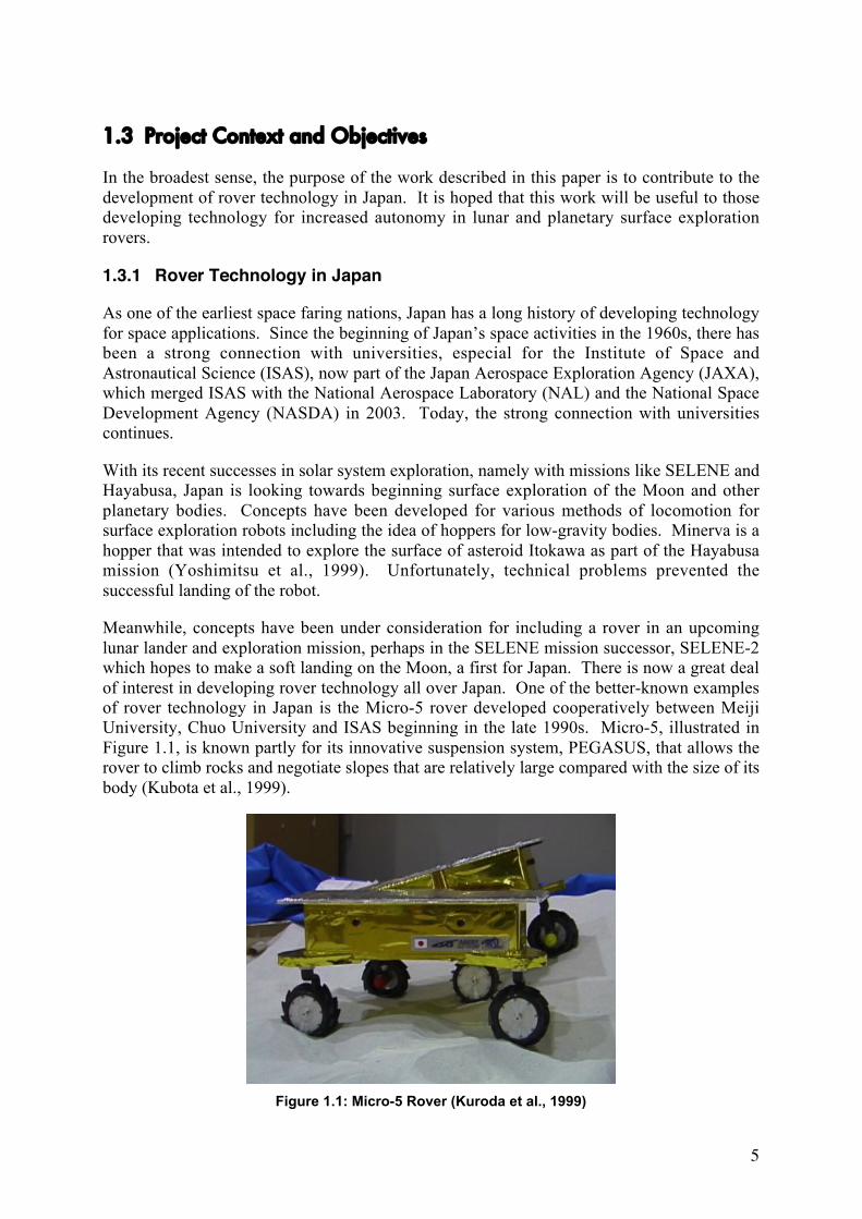
of rover technology in Japan is the Micro-5 rover developed cooperatively between Meiji
University, Chuo University and ISAS beginning in the late 1990s. Micro-5, illustrated in
Figure 1.1, is known partly for its innovative suspension system, PEGASUS, that allows the
rover to climb rocks and negotiate slopes that are relatively large compared with the size of its
body (Kubota et al., 1999).
Figure 1.1: Micro-5 Rover (Kuroda et al., 1999)
6
At the same time, other rover concepts are under development at institutions such as the
Tokyo Institute of Technology, Tohoku University and within JSpEC (JAXA Space
Exploration Center). Recently, ISAS, again in cooperation with Meiji and Chuo Universities,
has begun the development of a successor to the Micro-5, which they call M6. The M6 rover
is a much larger vehicle, approximately the size of the MERs, with a mast to support its main
sensors, two small forward reaching robotic arms, wheels that can be steered, generous
ground clearance and another innovative suspension system. Each of the three participating
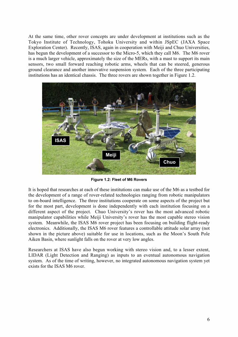
institutions has an identical chassis. The three rovers are shown together in Figure 1.2.
Figure 1.2: Fleet of M6 Rovers
It is hoped that researches at each of these institutions can make use of the M6 as a testbed for
the development of a range of rover-related technologies ranging from robotic manipulators
to on-board intelligence. The three institutions cooperate on some aspects of the project but
for the most part, development is done independently with each institution focusing on a
different aspect of the project. Chuo University’s rover has the most advanced robotic
manipulator capabilities while Meiji University’s rover has the most capable stereo vision
system. Meanwhile, the ISAS M6 rover project has been focusing on building flight-ready
electronics. Additionally, the ISAS M6 rover features a controllable attitude solar array (not
shown in the picture above) suitable for use in locations, such as the Moon’s South Pole
Aiken Basin, where sunlight falls on the rover at very low angles.
Researchers at ISAS have also begun working with stereo vision and, to a lesser extent,
LIDAR (Light Detection and Ranging) as inputs to an eventual autonomous navigation
system. As of the time of writing, however, no integrated autonomous navigation system yet
exists for the ISAS M6 rover.
ISAS
Meiji
Chuo
7
1.3.2 Stereo Vision and LIDAR for Navigation
Eventually, an autonomous navigation system will be developed for the ISAS M6 rover
including path planning and obstacle avoidance and may make use of a combination of stereo
vision and LIDAR inputs.
Stereo vision is already widely used in rovers, including on Mars Pathfinder’s Sojourner rover
and on the twin Mars Exploration Rovers (MERs) to extract 3D information from the robot’s
environment. The MERs use mast-mounted Navcam stereo cameras for general viewing and
global path planning while their local obstacle avoidance system uses lower-resolution, body-
mounted Hazcam stereo cameras instead. Unfortunately, these Hazcams have been
ineffective for Opportunity since it is operating in a region dominated by finely grained sand
that is impossible for the low-resolution Hazcams to resolve (Maimone et al., 2006). This
highlights one shortcoming of stereo vision, namely that it depends on the ability to identify
distinct features in the images. Another is the fact that its effectiveness depends heavily on
illumination of the scene, which relies entirely on light from the sun, and can suffer from
problems caused by low contrast or shadowing, for example.
LIDAR offers the advantage of not depending on sunlight to illuminate the scene. Instead,
laser pulses are actively reflected off objects in the scene and based on time of flight of the
returning laser pulse, distance can be computed. LIDAR can be used to construct precise
models of the environment under any lighting conditions. On the other hand, LIDAR does
little to characterize the surface appearance of the objects it views – a weakness in terms of
value for scientific analysis. Since it depends on the strength of the reflected signal, LIDAR
is effective only over a limited range. Thus, while LIDAR is useful for helping a robot model
its 3D environment, especially in its immediate vicinity, LIDAR alone is not sufficient for
scientific exploration missions. The best solution will likely be some combination of stereo
vision and LIDAR, capitalizing on the strengths of each.
1.3.3 Scope and Objectives
It is the author’s goal to make a real contribution to autonomous navigation research at ISAS
by doing more than simply conducting a study of the topic. Instead, the author’s goal has
been to provide a working, albeit basic, autonomous navigation system with the expectation
that the system will be augmented, expanded, and improved upon in the future. Such a
system would comprise data acquisition hardware as well as software for interfacing with the
sensor, storing data about the robot’s environment, identifying obstacles within that
environment, planning obstacle-avoiding trajectories, and communicating navigation
information to the robot’s motion control software.
8
The previously described M6 rover project is the perfect platform for demonstrating this kind
of system. The rover is physically nearly complete and includes a mast designed for
mounting of the primary navigation sensors: a stereo camera pair and a Laser Range Finder
(LRF) for LIDAR. Since another colleague is already focusing on the stereo vision system,
the work described in this report aims instead to employ the LRF as a primary sensor. A
secondary goal of this work is thus verifying the effectiveness of using LIDAR for this
application. Despite the initial focus on the LRF as the primary sensor, the system is
designed with the expectation that stereo vision will be integrated at a later date. The system
described in this report is by no means limited to this one particular robot, the M6 rover,
however, its prototype implementation does involve communication with the M6 rover’s
main On-Board Computer (OBC) and implementation on another system would require some
tailoring.
Since an LRF unit was already available for this project, the focus of the work described here
is on the software that processes the sensor data and ultimately produces navigation
instructions for the robot. Throughout the report, this software will generally be referred to as
the “navigation system”.
In order to satisfy the goal that this navigation system can be augmented, expanded and
improved upon in the future, it has been designed to be modular and configurable. This way,
an individual component can be swapped out with another one at any time, with little impact
to the overall functioning of the system. For example, should a researcher wish to test an
alternative method for modeling the terrain, it should be possible to do so without having to
significantly modify upstream or downstream components. Furthermore, should a researcher
wish to add a capability to the system such as localization (see section 4.2.3), it should be
possible to do so with little or no impact on the rest of the system.
This navigation system is meant only to provide researchers with a working starting point: a
testbed on which new algorithms and concepts can be tested in field trials. It is the author’s
view that new techniques and algorithms will mature far more rapidly and with greater
confidence through field trials rather than in mere computer simulations. Thus, the fact that
the system is working in an integrated manner is more important than the sophistication or
optimality of any of its components.
In order to motivate the realization of the project goals within the short time available, the
author chose a concrete target date for delivery of a working system: the ISAS Open House
on July 25, 2009. The Open House is an event hosted annually by ISAS during which the
facility’s doors are opened to the public. The event includes presentations and
demonstrations concerning a variety of engineering and science topics. This year, one such
demonstration included the three M6 rovers performing various tasks on an obstacle-strewn
field simulating a planetary surface. The author’s goal was to provide a navigation system
capable of instructing the ISAS M6 rover on how to avoid obstacles as it navigated the
simulated planetary surface during the demonstrations on July 25.
The scope of this project was limited to what was necessary to achieve a basic, working
obstacle-avoiding navigation tool in time for the ISAS Open House. No attempt was made to
develop any higher-level behaviour planning software such as task prioritization and
sequencing or automated supervisory systems for monitoring robot health and the like. The
intention was merely to have a working robot capable of spotting rocks or boulders in its path
and navigating around them.

9
2 System Concepts
This chapter begins by introducing the concept of operations for an autonomous rover and
identifying the role of the navigation system within it. From there, the navigation problem is
clarified and broken down into parts before discussing the key assumptions and approaches
that were employed. The chapter concludes with an overview of the resulting navigation
system and its components.
2.1 Operations Concept
Before discussing the details of the navigation system that has been developed, some context
is required. The purpose of the M6 rover project is to facilitate the development of rover
technology for lunar and planetary exploration. Lunar or planetary rovers will be sent first to
conduct scientific study and later to scout for upcoming human exploration missions. In
either case, the need for autonomy demands some high-level software to direct the actions of
the robot.
2.1.1 Behaviour Layers
At the highest level, Earth-based mission controllers will assign the robot’s tasks. A typical
assignment might be to search for and study any interesting rock samples in a given area.
Ideally, the robot could accept such a high-level command and could break it down into
smaller parts. The robot would be able to plan its approach, prioritize its actions and monitor
its own performance.
This kind of intelligence can be implemented in a 3-layer architecture. Typically, the top
layer handles planning and high-level decisions for the robot, the middle layer takes care of
executing specific tasks that are derived from those plans, and finally the bottom layer uses
the robot’s fundamental capabilities, such as capturing data from sensors and commanding
motion of actuators, to accomplish those tasks (Alami et al., 1998).
Initially based on this concept, engineers at JPL have been developing increasingly capable
architectures for rover autonomy (Estlin et al., 2007; Castaño et al., 2007). They have
developed a system called OASIS (Onboard Autonomous Science Investigation System),
whose aim it is to not only improve automatic handling of unexpected problems but also to
take advantage of serendipitous science opportunities that might arise. For example, a rover
on its way to some planned objective may come across a particularly interesting rock and may
choose to stop to take a closer look, and then re-prioritize its overall plan accordingly.
10
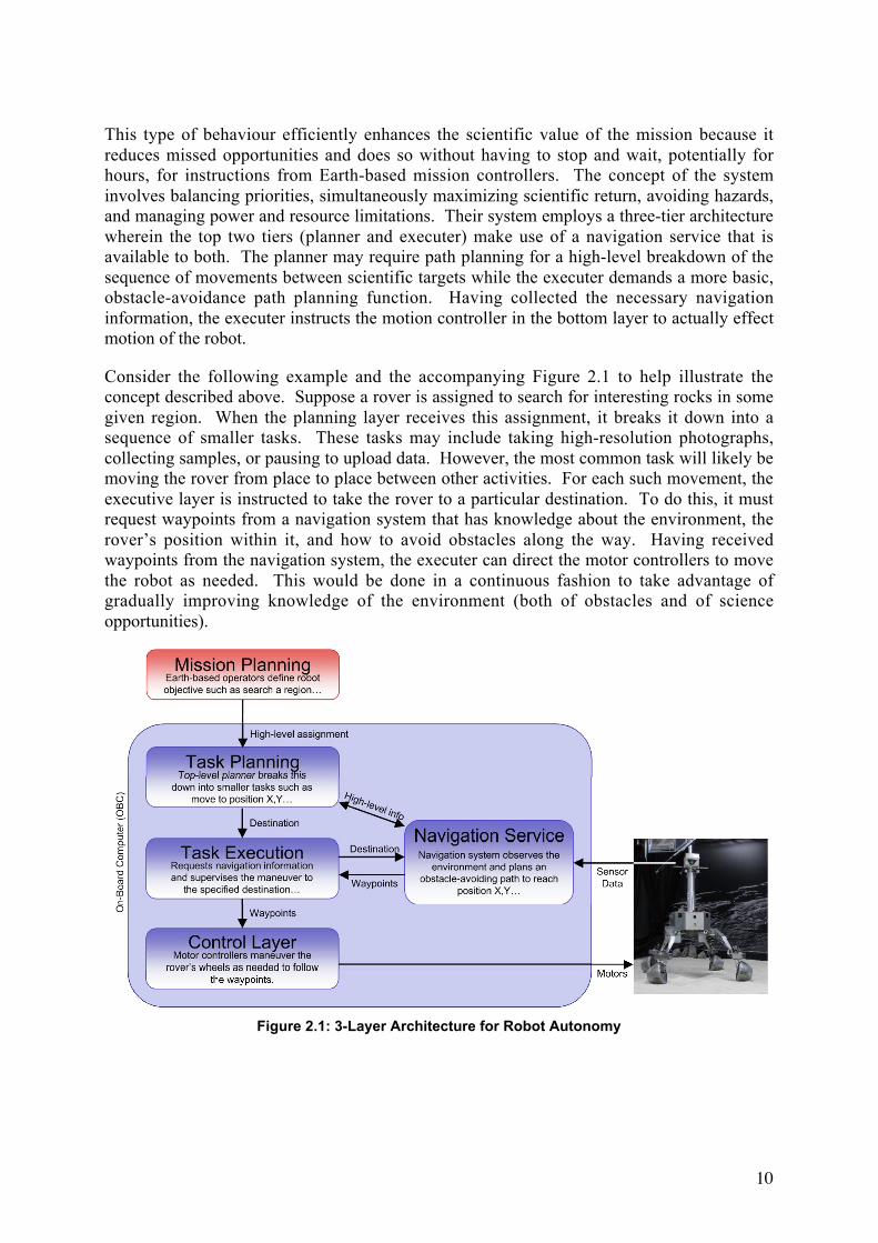
This type of behaviour efficiently enhances the scientific value of the mission because it
reduces missed opportunities and does so without having to stop and wait, potentially for
hours, for instructions from Earth-based mission controllers. The concept of the system
involves balancing priorities, simultaneously maximizing scientific return, avoiding hazards,
and managing power and resource limitations. Their system employs a three-tier architecture
wherein the top two tiers (planner and executer) make use of a navigation service that is
available to both. The planner may require path planning for a high-level breakdown of the
sequence of movements between scientific targets while the executer demands a more basic,
obstacle-avoidance path planning function. Having collected the necessary navigation
information, the executer instructs the motion controller in the bottom layer to actually effect
motion of the robot.
Consider the following example and the accompanying Figure 2.1 to help illustrate the
concept described above. Suppose a rover is assigned to search for interesting rocks in some
given region. When the planning layer receives this assignment, it breaks it down into a
sequence of smaller tasks. These tasks may include taking high-resolution photographs,
collecting samples, or pausing to upload data. However, the most common task will likely be
moving the rover from place to place between other activities. For each such movement, the
executive layer is instructed to take the rover to a particular destination. To do this, it must
request waypoints from a navigation system that has knowledge about the environment, the
rover’s position within it, and how to avoid obstacles along the way. Having received
waypoints from the navigation system, the executer can direct the motor controllers to move
the robot as needed. This would be done in a continuous fashion to take advantage of
gradually improving knowledge of the environment (both of obstacles and of science
opportunities).
Figure 2.1: 3-Layer Architecture for Robot Autonomy
11
The navigation system can be thought of as a basic capability or service that is provided to the
robot’s higher-level intelligences. The navigation system is capable of collecting information
about its environment mainly through sensors. The system models that environment in some
useful way and when queried, can provide information needed by the planning and execution
software. Note that during execution of a maneuver, it may be useful to have the navigation
system alert the executer or update the planned path as new information becomes available (in
case a previously undetected obstacle appears in the path, for example).
2.1.2 M6 Rover Operations
Although the M6 rover project could theoretically employ the behaviour layer concepts
presented in the preceding section, no such thing has yet been implemented. There is
currently no top-level robot behaviour planning system that prioritizes and sequences the
robot’s tasks, nor an executer to give the navigation system its orders. These layers of
autonomy can surely be added at a later date, with the navigation service integrated properly
on the On-Board Computer (OBC). But in the meantime, an alternative arrangement is
required.
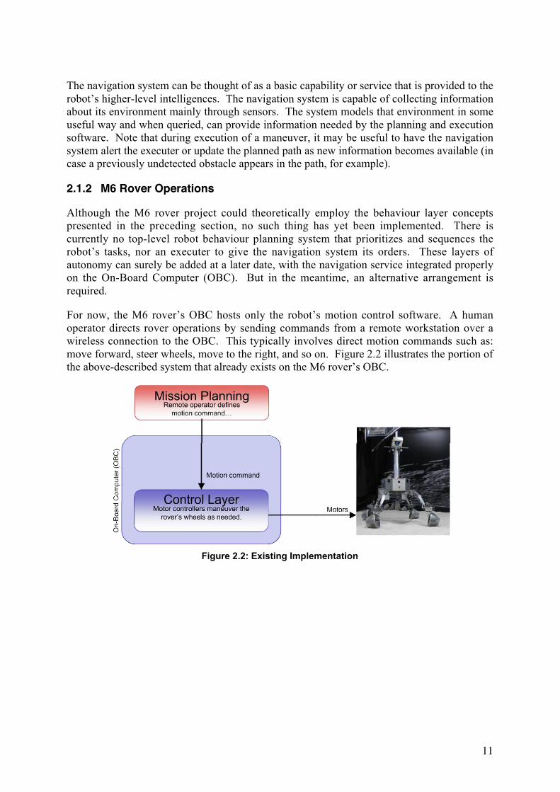
For now, the M6 rover’s OBC hosts only the robot’s motion control software. A human
operator directs rover operations by sending commands from a remote workstation over a
wireless connection to the OBC. This typically involves direct motion commands such as:
move forward, steer wheels, move to the right, and so on. Figure 2.2 illustrates the portion of
the above-described system that already exists on the M6 rover’s OBC.
Figure 2.2: Existing Implementation

12
In order to accommodate the integration and testing of the autonomous navigation system
described here, functionality was added to the OBC to interface between its existing motion
control capabilities and the waypoint-planning service provided by the navigation system.
For now, the navigation system runs as a standalone program on a separate computer and
interfaces with the OBC via TCP/IP over Ethernet. This temporary interface code added to
the OBC effectively takes the place of the higher-level task planning and execution software
by supplying the navigation system with destination coordinates and accepting and following
the waypoints it returns. Of course, without the real task planning software in place, the
selection of destination coordinates could not be determined autonomously. Instead, a human
operator working from a remote workstation would supply the destination coordinates. The
waypoints returned by the navigation software could be followed autonomously by the OBC’s
motion control software, provided that the OBC’s functionality included the ability to know
the rover’s position (see section 2.3.2 for more detail). As it relates to the previous two
diagrams, the system implemented as of the ISAS Open House, is shown in Figure 2.3.
Figure 2.3: Navigation System Testing Implementation
Because the navigation system runs on a separate computer, it does not have direct access to
the OBC’s position estimation information. The TCP/IP interface between the two computers
was therefore designed to have the OBC provide the navigation system with both destination
coordinates and the rover’s estimated current position (both in some absolute frame of
reference). The navigation computer responds to each with an updated next waypoint
(specified in the same absolute coordinate frame) accounting for the latest information about
the environment, the rover’s position within it, and its latest intended destination.
13
2.2 Problem Definition
The principal technical objective of this project has been to deliver a navigation system
capable of observing a scene using a Laser Range Finder (LRF) and ultimately providing
obstacle-avoiding navigation instructions to the ISAS M6 rover’s On-Board Computer
(OBC).
This problem can be broken down into the following parts:
1. Sensing: Use the LRF to collect data from the environment. This involves interfacing
the LRF device with the computer software and processing the raw data into
something meaningful. The result is an array of distance measurements in spherical
coordinates from the perspective of the sensor.
2. Modelling or Mapping: Use the LRF data to make a 3D model of the environment.
This requires transforming the incoming data from the spherical coordinates of the
sensor into Cartesian coordinates suitable for mapping. From this, construct a map of
the robot’s environment based on the 3D scene model. This involves gathering scene
model data over time and building an ever more complete map of the robot’s
environment.
3. Terrain Assessment and “Costing” for Obstacle Detection: Determine the
difficulty or “cost” associated with traversing given portions of the map. This is how
obstacles or dangerous terrain are identified.
4. Path Planning: Considering the dimensions of the robot, find a path to a specified
destination that avoids parts of the map that are not traversable (i.e. where the cost is
too high).
5. Direct the Rover’s Motion: Based on the planned path, provide the rover’s On-Board
Computer (OBC) with waypoints to direct its motion away from obstacles.
2.3 Assumptions
In this section, each of the parts of the problem is examined briefly and assumptions are
identified. Where it is warranted, explanations are given to justify the validity of the
assumptions or their suitability to the problem at hand.
2.3.1 Sensing
Naturally, some noise and errors are expected in the resulting data but it is generally assumed
that the LRF’s built-in time of flight calculations result in reasonably accurate distance
measurements. Since the focus of this work is to develop an end-to-end working system with
the potential for upgrading its individual components later, no significant or systematic effort
was conducted to characterize the accuracy or precision of the LRF. As part of future work,
this could be examined more closely with the sensor being properly characterized, or if a
better LIDAR unit becomes available, possibly replaced altogether.
14
2.3.2 Modelling and Mapping
The robot is assumed to begin with little or no information about its environment. Its model
of the environment will gradually improve over time as it explores. This assumption implies
a need to accumulate environmental data over time and store it in an integrated model. This,
in turn, implies a need for a consistent frame of reference so that multiple sensor
measurements can be combined in a coherent fashion.
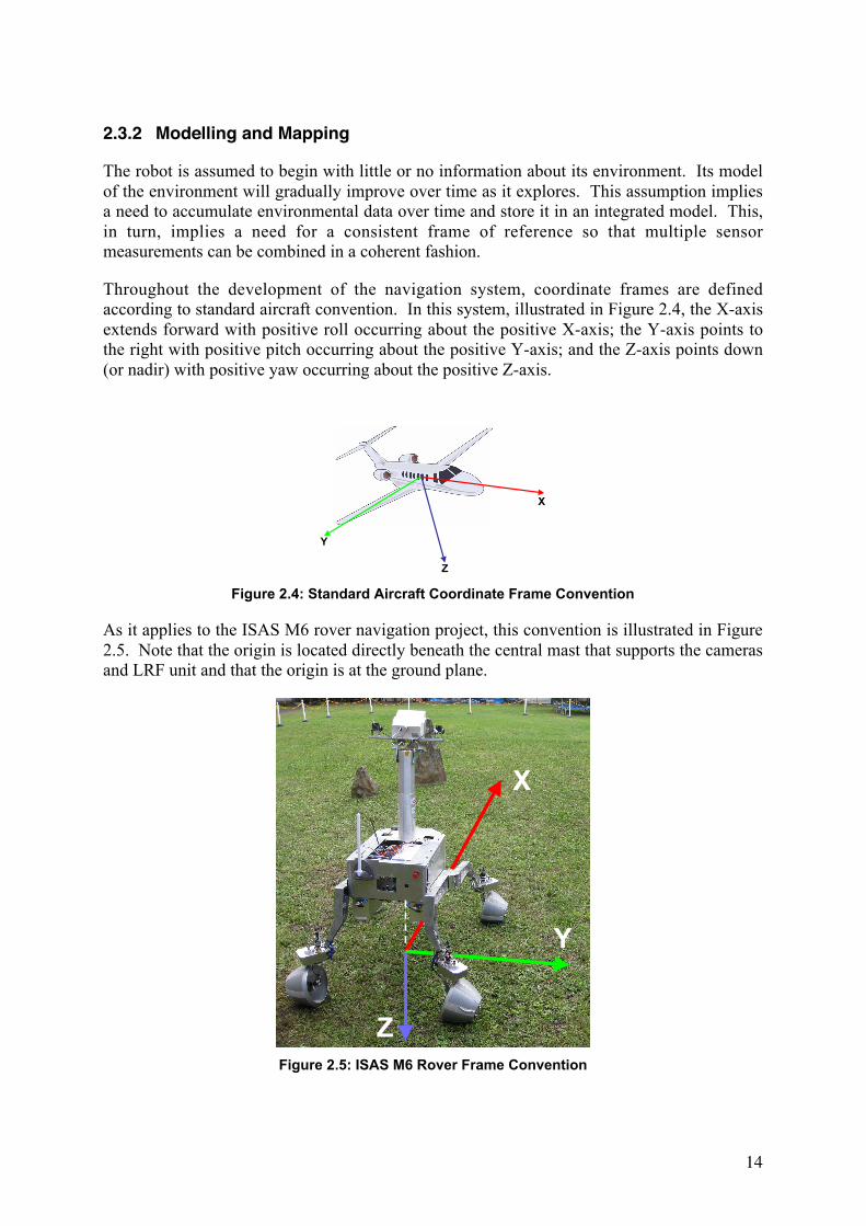
Throughout the development of the navigation system, coordinate frames are defined
according to standard aircraft convention. In this system, illustrated in Figure 2.4, the X-axis
extends forward with positive roll occurring about the positive X-axis; the Y-axis points to
the right with positive pitch occurring about the positive Y-axis; and the Z-axis points down
(or nadir) with positive yaw occurring about the positive Z-axis.
Z
X
Y
Figure 2.4: Standard Aircraft Coordinate Frame Convention
As it applies to the ISAS M6 rover navigation project, this convention is illustrated in Figure
2.5. Note that the origin is located directly beneath the central mast that supports the cameras
and LRF unit and that the origin is at the ground plane.
Z
X
Y
Figure 2.5: ISAS M6 Rover Frame Convention
15
Assuming the sensor provides position measurements in spherical coordinates, transforming
the data points into Cartesian coordinates is relatively straightforward and produces a cloud of
points expressed with respect to a coordinate frame centered on the sensor. In order to
transform this data into some absolute frame of reference for mapping purposes, the
navigation system must know both the pose (position and orientation) of the robot with
respect to that absolute reference frame as well as the pose of the sensor with respect to the
robot itself. Both of these pieces of information are assumed to be available to the navigation
system. Finally, to plan a path to a destination, the navigation system needs destination
coordinates to be provided, once again, in that same absolute reference frame.
Note, however, that obtaining an accurate estimate of the rover’s position is not trivial.
Hence, these fundamental assumptions are somewhat threatened and it is worth identifying
the potential consequences should a reliable position estimation functionality be absent.
Firstly, without rover position data, it will be impossible for the navigation system to
accumulate environmental knowledge over time. Two measurements taken from different
positions could not be combined into a single model or map unless those two positions were
known, at least with respect to each other. This means that the robot could never have
knowledge of areas beyond the immediate vicinity of the sensor. Furthermore, a navigation
system could, in theory accept a destination relative to its current position and plan a path
toward that point. But as soon as the rover starts moving, the previously identified destination
coordinates are no longer meaningful (since they will shift with the rover). This means that
the navigation system will be unable to update that path in the event that a previously
undetected obstacle is observed along the way. A problem made all the more likely by the
fact that the system’s environmental knowledge is limited to the small area immediately in
front of the rover.
2.3.3 Terrain Assessment and Costing
Costing essentially just means assigning a cost to areas of the map based on the perceived
difficulty of traversing those parts of the robot’s environment. Costing is used by path
planning algorithms to find an acceptable route from one point to another. The cost of
traversing smooth and level terrain should be low while the cost of traversing over very steep
or rough terrain, or through obstacles should be very high, if not infinite (to be sure the
planned path will not pass through an obstacle; see section 3.3 for details). Determination of
costs is partly a function of the rover’s size and terrain negotiation capabilities because what
is an obstacle for a small rover may not be an obstacle for a larger rover with larger wheels or
more ground clearance, for example. For purposes of M6 rover path planning, it is assumed
that the rover can overcome small rocks but that any objects rising more than 15 cm above the
ground plane should be considered obstacles.
The robot cannot be assumed to be positioned at a single point since this could result in a path
planned between two rocks that are too narrowly spaced to allow the rover to squeeze
between them. Instead, the full breadth of the robot’s footprint is considered. Because the
M6 rover has fairly high ground clearance, it is theoretically possible for it to straddle rocks
that are too large for the wheels to climb but small enough to pass safely beneath the robot’s
belly. A sophisticated approach to costing might separately assess the costs of wheel versus
body traversal. However, this will be left as future work. For simplicity in this prototype
implementation, the rover is assumed to occupy all the space beneath it.
16
2.3.4 Path Planning
An intuitive approach to path planning is to build a grid-based map of the robot’s
environment and assign costs to each cell in the grid. Cell costs would be relatively low in
flat terrain but very high where obstacles are located. Unknown cells (in regions that have not
yet been observed by the sensor) may be assigned a very high or infinite cost. This prevents
the robot from planning any paths through unknown and therefore potentially unsafe areas.
At first glance, this seems like a sensible approach to path planning. However, if a robot has
only sparse information about its environment, this approach is very restrictive. It means that
the robot cannot even attempt to go to an unexplored area. If the robot’s purpose is to explore
an unfamiliar planetary surface, this is obviously not acceptable.
For a robot that is exploring mostly unknown territory, it is more than reasonable to assume
that the robot will not have sufficient knowledge to plan a path all the way to its destination
without traversing any unknown areas. Indeed, the destination itself may be in an as-yet
unknown area. It is also reasonable to assume that the robot will have to dynamically adjust
the planned course as it learns more about its environment. If an obstacle appears to be in the
way, the path needs to be adjusted. This last assumption implies that the robot has to be able
to detect previously unknown obstacles as it approaches them. In other words, the robot must
have good and frequently updated knowledge of the area immediately in front of it.
A look at the way humans operate in unfamiliar environments illustrates why this approach is
entirely sensible. Suppose a man is outside a department store, and sees through the window,
a desirable item. If the man does not know the area, the most efficient route to get into the
store is probably not known. Assuming the item is sufficiently compelling, this lack of
knowledge will not cause the man to give up. Instead, he will venture into unknown territory
in search of an entrance. He may make a starting assumption and plan a tentative path to
follow. The man can do this with confidence because although he cannot be certain his
assumed path will work out, he is watching where he is going and knows that he is capable of
adjusting his plan as he goes. These exact same principles have been applied to the path
planning system described here.
For purposes of designing a path-planning algorithm, a few additional assumptions were
made. In particular, it has been assumed that the robot’s environment consists mostly of
navigable areas with obstacles and impassible terrain forming islands in an otherwise clear
workspace. In other words, the task of the path-planning algorithm is to find a path around
obstacles strewn in the rover’s workspace rather than to tunnel through a labyrinth. This is
important because it affects the choice of path planning algorithm, as some are more suited to
one type of environment or the other.
As discussed in the costing assumptions, the rover is assumed to occupy its entire footprint
area. For the prototype implementation, this footprint is assumed to be wide enough to allow
the robot’s heading to be ignored. This choice is based on the fact that the M6 rover, unlike a
car, is holonomic, meaning that its heading is not strictly tied to its direction of motion.
17
2.3.5 Directing the Rover
From the point of view of communication, the navigation system relies on the assumption that
it will receive TCP/IP packets from the OBC describing the latest rover pose and the latest
desired destination coordinates, both in the absolute reference frame. With this information
and its access to the LRF device, the navigation system can build its model of the
environment, plan a path to the destination coordinates and respond to the OBC with a
TCP/IP packet containing the next waypoint on the planned path. As the robot moves, the
OBC will continue to provide updated rover pose estimates (again, assumed to be reliable)
and with each update, will receive a new next waypoint from the navigation computer in
return. In this way, the rover is always working towards the nearest waypoint on the way to
the specified destination and this waypoint is always based on the latest available model of
the environment. Pose updates from the OBC are expected at a frequency of up to about 1Hz.
This high frequency of updates is required to ensure that newly viewed obstacles can be
avoided.
2.3.6 Summary of Key Assumptions
For convenience, the key assumptions described in the preceding sections are summarized
below.
1. The LRF measures points in a spherical coordinate system centered at the sensor.
2. The LRF measurements are sufficiently accurate for purposes of this work. No
deliberate calibration effort has been undertaken.
3. The robot begins with little or no information about its environment.
4. The robot gradually accumulates knowledge of its environment over time.
5. The navigation system models the environment in Cartesian space using some
absolute frame of reference.
6. The navigation system has available to it, the pose of the robot with respect to the
same absolute frame of reference.
7. The navigation system has available to it, the pose of the sensor with respect to the
robot.
8. The intended destination coordinates are provided to the navigation system with
respect to the absolute frame of reference.
9. Any rock or abrupt change in surface elevation greater than 15 cm in height is
considered to be an obstacle.
10. The robot does not generally have sufficient knowledge to guarantee a clear path all
the way to its destination, which may lie outside all known areas.
11. The robot will adjust the planned course dynamically as it learns more about the
environment.
12. The robot’s sensors have a good view of the area immediately in front of the rover.
13. The forward-viewing sensors are used often enough to detect obstacles as the robot
approaches them.
18
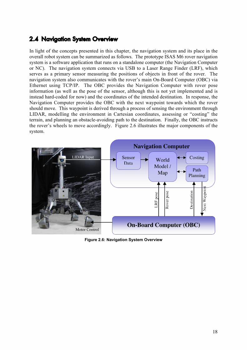
2.4 Navigation System Overview
In light of the concepts presented in this chapter, the navigation system and its place in the
overall robot system can be summarized as follows. The prototype ISAS M6 rover navigation
system is a software application that runs on a standalone computer (the Navigation Computer
or NC). The navigation system connects via USB to a Laser Range Finder (LRF), which
serves as a primary sensor measuring the positions of objects in front of the rover. The
navigation system also communicates with the rover’s main On-Board Computer (OBC) via
Ethernet using TCP/IP. The OBC provides the Navigation Computer with rover pose
information (as well as the pose of the sensor, although this is not yet implemented and is
instead hard-coded for now) and the coordinates of the intended destination. In response, the
Navigation Computer provides the OBC with the next waypoint towards which the rover
should move. This waypoint is derived through a process of sensing the environment through
LIDAR, modelling the environment in Cartesian coordinates, assessing or “costing” the
terrain, and planning an obstacle-avoiding path to the destination. Finally, the OBC instructs
the rover’s wheels to move accordingly. Figure 2.6 illustrates the major components of the
system.
Figure 2.6: Navigation System Overview
19
3 Implementation
This chapter examines the implementation details of each of the navigation system
components. Relevant research is discussed as various implementation options are
considered. The system was developed using the C programming language and only a
minimal set of basic libraries. Auxiliary programs were developed to support communication
testing and visualization but otherwise, the core of the system was implemented as a single
application operating on the Linux ubuntu operating system. Although a significant portion
of the effort of the work discussed here involved implementation challenges, these are not
discussed here. Instead, this section concentrates only on the core issues and algorithms.
3.1 Sensing
The first component in the navigation system is the collection of data about the robot’s
environment. Although the navigation system may theoretically accept input from various
different types of sensors, the prototype implementation discussed here uses only LIDAR.
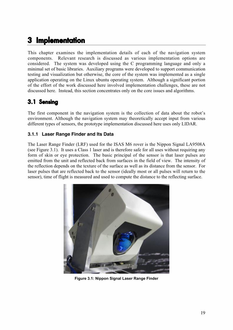
3.1.1 Laser Range Finder and Its Data
The Laser Range Finder (LRF) used for the ISAS M6 rover is the Nippon Signal LA9508A
(see Figure 3.1). It uses a Class 1 laser and is therefore safe for all uses without requiring any
form of skin or eye protection. The basic principal of the sensor is that laser pulses are
emitted from the unit and reflected back from surfaces in the field of view. The intensity of
the reflection depends on the texture of the surface as well as its distance from the sensor. For
laser pulses that are reflected back to the sensor (ideally most or all pulses will return to the
sensor), time of flight is measured and used to compute the distance to the reflecting surface.
Figure 3.1: Nippon Signal Laser Range Finder

20
The unit completes a scan over a 60º x 60º field of view by reflecting the beam of the
stationary laser off a rapidly rotating mirror (see Figure 3.2). As the pulsing laser beam is
swept over the field of view, distance and reflectivity measurements are recorded for each
pulse. This results in a square grid of 105 x 105 discrete measurements. The scanner
operates continually, replacing the scan data in its on-board memory buffer approximately
once every 0.8 seconds. The device is connected to a computer via USB. The C-language
source code used for the navigation system implementation uses standard USB libraries to
communicate with the device, collecting the latest scan results whenever needed.
Figure 3.2: Rotating Mirror inside LRF
Since the laser beam is always emitted from precisely the same point and is reflected off the
centre of the rotating mirror, the resulting distance measurements effectively give the
positions of every point in the field of view (minus those that do not sufficiently reflect the
laser pulse) in spherical coordinates with the origin at the centre of the reflecting mirror.
21
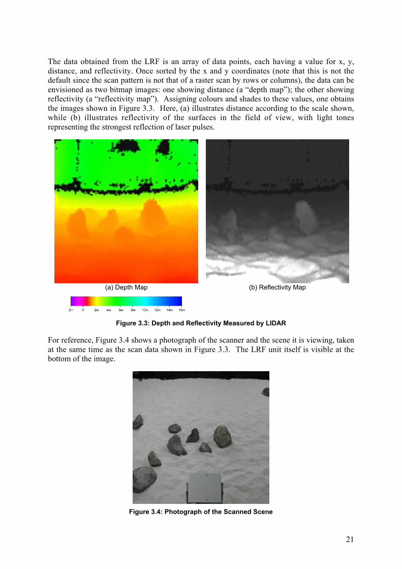
The data obtained from the LRF is an array of data points, each having a value for x, y,
distance, and reflectivity. Once sorted by the x and y coordinates (note that this is not the
default since the scan pattern is not that of a raster scan by rows or columns), the data can be
envisioned as two bitmap images: one showing distance (a “depth map”); the other showing
reflectivity (a “reflectivity map”). Assigning colours and shades to these values, one obtains
the images shown in Figure 3.3. Here, (a) illustrates distance according to the scale shown,
while (b) illustrates reflectivity of the surfaces in the field of view, with light tones
representing the strongest reflection of laser pulses.
(a) Depth Map (b) Reflectivity Map
Figure 3.3: Depth and Reflectivity Measured by LIDAR
For reference, Figure 3.4 shows a photograph of the scanner and the scene it is viewing, taken
at the same time as the scan data shown in Figure 3.3. The LRF unit itself is visible at the
bottom of the image.
Figure 3.4: Photograph of the Scanned Scene

22
3.1.2 Noise and Filtering
Unfortunately, the data supplied by the LRF is not always ready to use as-is. The LRF data
can sometimes contain artifacts giving the appearance of very near or very distant objects that
are in fact, not present at all. When the lens is dirty, distance estimates can be highly
inaccurate especially in areas with poor reflection. This is an important result because for
remote rovers, there will be no opportunity to clean the lens unless such a capability is
somehow built-in.
Regardless of the source of error, it is important to eliminate non-credible measurements from
the LRF data to avoid modelling phantom objects in the robot’s environment. Some simple
techniques were tried early in the implementation process including elimination of objects
that appear to be unrealistically near or far or surfaces that reflect very poorly, since this is
often associated with inaccurate distance estimates. These techniques proved too simplistic,
however, as they were not always capable of removing bad data without also removing some
good data. A look at the relationship between measured distance and reflectivity, hints at the
problem (see Figure 3.5).
LRF scan before filter
0
500
1000
1500
2000
2500
3000
-2 0 2 4 6 8 10 12 14 16
Distance (m)
Reflectivity
Figure 3.5: Non-credible Data Points in Raw LRF Data
Naturally, objects that are nearest to the sensor tend to reflect more brightly than do distant
objects. This suggests a natural distribution of data points with something like a negative
exponential shape. The data points highlighted in red lie outside the main family of data
points and thus seem less credible. Indeed, some of the points in the cluster near the origin
exhibit negative distance estimates, which of course is impossible. Similarly, there are data
points that appear to lie beyond the far wall of the room in which the tests were conducted.
23
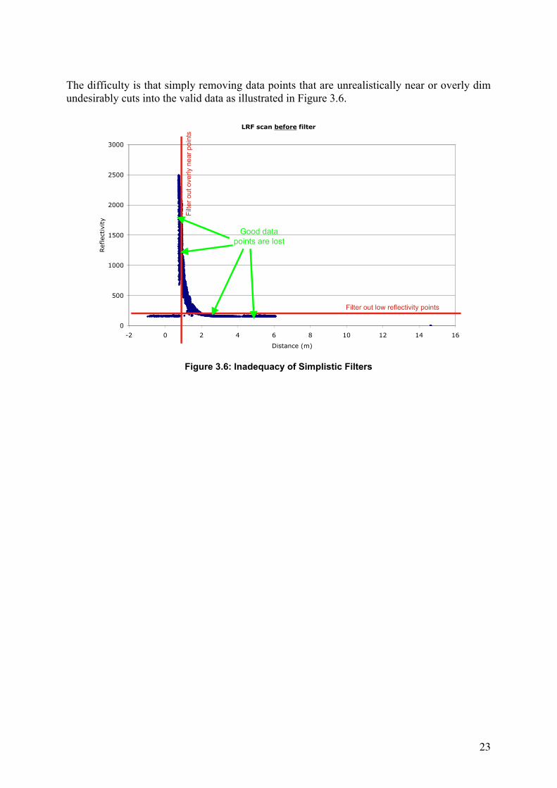
The difficulty is that simply removing data points that are unrealistically near or overly dim
undesirably cuts into the valid data as illustrated in Figure 3.6.
LRF scan before filter
0
500
1000
1500
2000
2500
3000
-2 0 2 4 6 8 10 12 14 16
Distance (m)
Reflectivity
Filter out low reflectivity points
Filt
er
out overly n
ear
poin
ts
Good data
points are lost
Figure 3.6: Inadequacy of Simplistic Filters
24
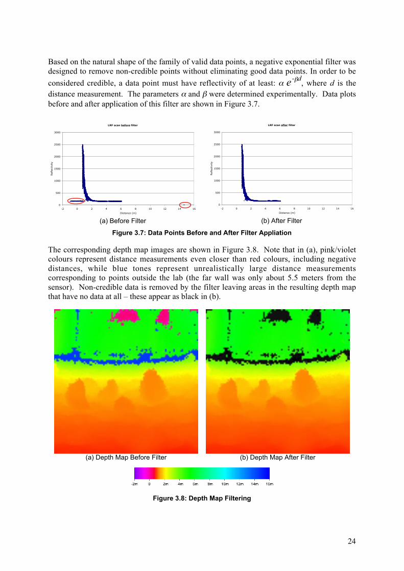
Based on the natural shape of the family of valid data points, a negative exponential filter was
designed to remove non-credible points without eliminating good data points. In order to be
considered credible, a data point must have reflectivity of at least: " e-#d
, where d is the
distance measurement. The parameters " and # were determined experimentally. Data plots
before and after application of this filter are shown in Figure 3.7.
LRF scan before filter
0
500
1000
1500
2000
2500
3000
-2 0 2 4 6 8 10 12 14 16
Distance (m)
Reflectivity
(a) Before Filter
LRF scan after filter
0
500
1000
1500
2000
2500
3000
-2 0 2 4 6 8 10 12 14 16
Distance (m)Reflectivity
(b) After Filter
Figure 3.7: Data Points Before and After Filter Appliation
The corresponding depth map images are shown in Figure 3.8. Note that in (a), pink/violet
colours represent distance measurements even closer than red colours, including negative
distances, while blue tones represent unrealistically large distance measurements
corresponding to points outside the lab (the far wall was only about 5.5 meters from the
sensor). Non-credible data is removed by the filter leaving areas in the resulting depth map
that have no data at all – these appear as black in (b).
(a) Depth Map Before Filter (b) Depth Map After Filter
Figure 3.8: Depth Map Filtering

25
3.2 Modelling and Mapping
In order to make use of the set of point measurements collected by the sensor, the data needs
to be organized into some coherent structure that is suitable for geometric analysis and
ultimately, for path planning purposes. The first problem is that the data is represented only
as a depth map. This must be converted into a Cartesian space representation. Since the
result is a Cartesian space cloud of points that is not organized in any useful way, the problem
then becomes organizing the data into a format that is related to the layout of the robot’s
environment.
3.2.1 Transforming the Sensor Data into Cartesian Space
The transformation from depth map to Cartesian space point cloud requires a few steps of
relatively straightforward trigonometry. First, a coordinate frame convention must be
established. As explained in the assumptions (see section 2.3.2), standard aircraft convention
has been applied throughout the navigation system. Correspondingly, the Cartesian frame
applied to the sensor is as illustrated in Figure 3.9. Now, consider an arbitrary point P, in the
sensor’s field of view. The goal is to find the Cartesian coordinates (x, y, z) of this point with
respect to the coordinate frame defined at the centre of the sensor.
Figure 3.9: Arbitrary Point, P, Relative to the Sensor
The LRF gives 3D coordinates of the point P, but expressed in spherical coordinates. In
spherical coordinates, the point P is expressed using three values, typically azimuth ($),
elevation (!), and radial distance (d, here). The distance, d, from the sensor to the point P is
available directly as the distance measurement given by the LRF. The azimuth ($) and
elevation (!), on the other hand, must be obtained based on the image pixel coordinate of the
point P. Knowing the pixel size (~0.57º for the LRF unit in question), the two angles can be
computed from the horizontal and vertical image pixel positions (respectively h and v) of
point P relative to the image centre (see Figure 3.10): $ = h * pixel_size, and ! = v *
pixel_size.
v
hImage
Centre
P
Figure 3.10: Aribtrary Point, P, as Seen in the Depth Map Image
26
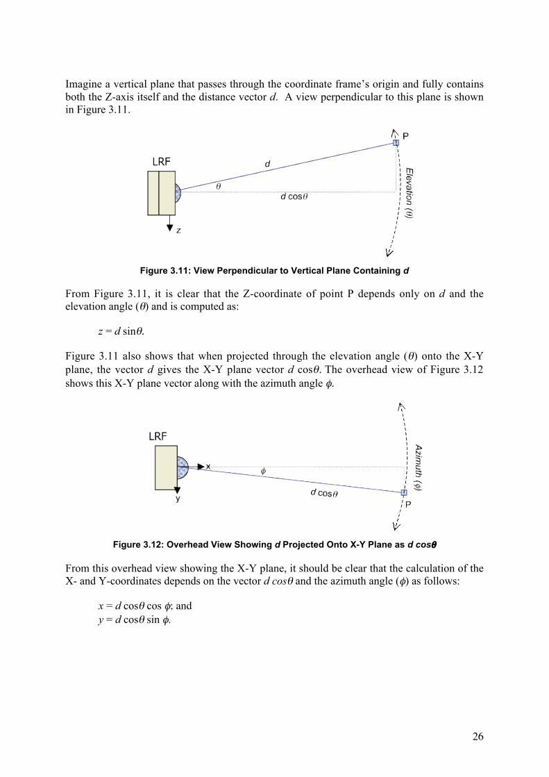
Imagine a vertical plane that passes through the coordinate frame’s origin and fully contains
both the Z-axis itself and the distance vector d. A view perpendicular to this plane is shown
in Figure 3.11.
Figure 3.11: View Perpendicular to Vertical Plane Containing d
From Figure 3.11, it is clear that the Z-coordinate of point P depends only on d and the
elevation angle (!) and is computed as:
z = d sin!.
Figure 3.11 also shows that when projected through the elevation angle (!) onto the X-Y
plane, the vector d gives the X-Y plane vector d cos!. The overhead view of Figure 3.12
shows this X-Y plane vector along with the azimuth angle $.
Figure 3.12: Overhead View Showing d Projected Onto X-Y Plane as d cos!
From this overhead view showing the X-Y plane, it should be clear that the calculation of the
X- and Y-coordinates depends on the vector d cos! and the azimuth angle ($) as follows:
x = d cos! cos $; and
y = d cos! sin $.
27
3.2.2 Cartesian Space Point Cloud
At this point, the positions of the point measurements are known in Cartesian coordinates
with respect to the sensor frame. But it is still necessary to transform from this frame to the
absolute reference frame in which the robot is operating. This step is accomplished using 4x4
homogeneous transformation matrices obtained from the known robot pose relative to the
absolute reference frame (Tabsref,robot
) and the known pose of the sensor relative to the robot
(Trobot,sensor
). The two transformations are computed from the known values for x, y, z, roll,
pitch, and yaw. The derivation for this is not shown here but the formula for the computation
can be found in the source code.
Once computed, the two matrices are multiplied together producing a single transformation
from the absolute reference frame to the sensor frame (Tabsref,sensor
= Tabsref,robot
Trobot,sensor
).
Finally, the point vector expressing the location of P in the sensor frame (vsensor,P
) can be
placed in the upper right corner of a 4x4 Identity matrix to form Tsensor,P
for use in the
following computation: Tabsref,P
= Tabsref,sensor
Tsensor,P
. The first three elements of the last
column of the resulting Tabsref,P
is the position vector vabsref,P
, giving the coordinates of P
relative to the absolute reference frame.
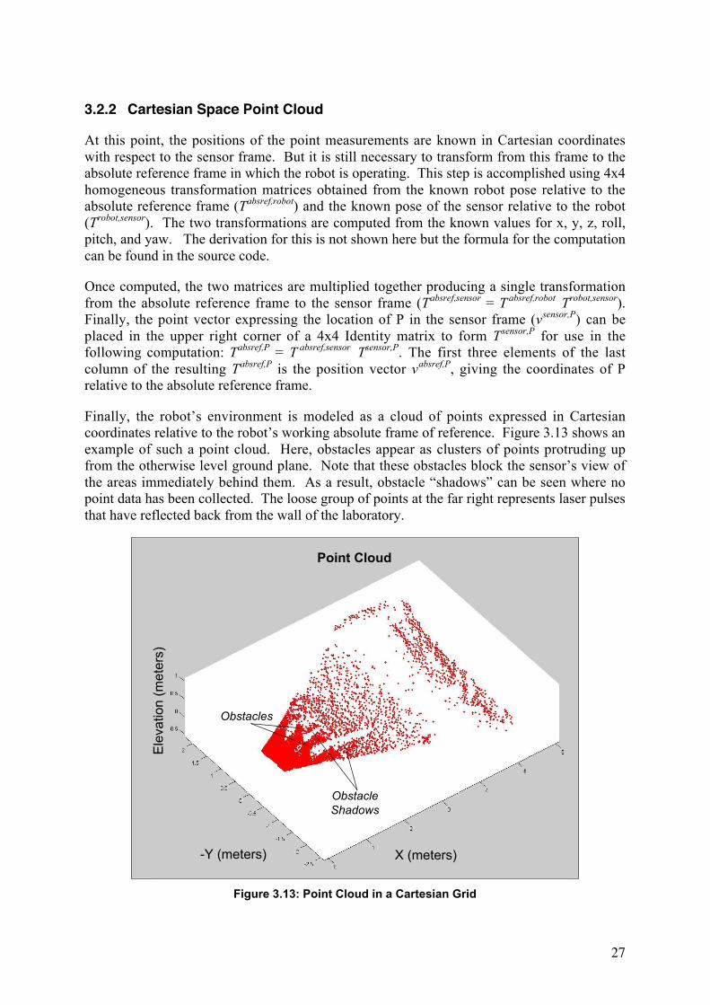
Finally, the robot’s environment is modeled as a cloud of points expressed in Cartesian
coordinates relative to the robot’s working absolute frame of reference. Figure 3.13 shows an
example of such a point cloud. Here, obstacles appear as clusters of points protruding up
from the otherwise level ground plane. Note that these obstacles block the sensor’s view of
the areas immediately behind them. As a result, obstacle “shadows” can be seen where no
point data has been collected. The loose group of points at the far right represents laser pulses
that have reflected back from the wall of the laboratory.
X (meters)
Point Cloud
Ele
va
tio
n (
me
ters
)
-Y (meters)
Obstacles
Obstacle
Shadows
Figure 3.13: Point Cloud in a Cartesian Grid

28
3.2.3 Model Format Options
The cloud of points discussed so far is an unorganized set of data in that it is a simple list of
coordinates and is not sorted in any way nor is it conveniently searchable. Before any terrain
analysis or path planning can be done, the data must be restructured into a map or world
model of some kind. The choice of data format depends on how the model will be used. For
efficiency, it may be practical to simplify the data, keeping only information that will be
important for the model’s ultimate purpose. On the other hand, some formats may do the
opposite, adding to the size of the data by identifying useful relationships between the points
in the original data cloud.
If the goal is to model a surface precisely, it may be appropriate to fit polygons to the points
in the cloud, generating a mesh that models the surfaces of objects in the scene. Rodríguez
Gonzálvez (2007) and Rekleitis, et al. (2009) have developed techniques for modelling
surfaces specifically based on LIDAR data. Rekleitis, et al. (2009) perform Delaunay
triangulation on the points and then decimate the resulting mesh by merging nearly coplanar
triangles in order to reduce the data to a more manageable set. This results in a high fidelity
model of the surfaces in the robot’s environment but it is a complex process and is
computationally intensive.
In some cases, it may be appropriate to model the robot’s environment in a topological
fashion. A robot that operates inside a house, for example, might maintain a graph with nodes
representing various rooms and edges connecting nodes only where it is possible to move
between those rooms. This conceptual approach may have some uses but does little to model
the geometry of the robot’s workspace and is thus not well suited to the obstacle avoidance
problem.

29
A more common approach is to define a grid over regular and definite Cartesian coordinates.
The result is a Digital Elevation Model (DEM), also called a Digital Terrain Model (DTM),
with a grid of cells over a 2D horizontal plane with each grid cell containing information
about the terrain in that area. Principally, the cell data includes the mean or maximum
elevation of the corresponding piece of terrain. Additional useful data can also be stored for
each cell depending on what information is available from the data collection. If the data
collection used photography, it may be possible to include colour and texture data in the cells
for photorealistic models such as those available in GoogleEarth. The Martian terrain
modeled in Figure 3.14 is based on satellite measurements and thus has somewhat course
resolution but the principle can be applied at arbitrarily higher resolutions.
Figure 3.14: Terrain Model of Candor Chasma, Mars (GoogleEarth, 2009)
Using DEMs has the advantage of being intuitive, straightforward to implement, easy to work
with and of keeping the data compact. Disadvantages include the fact that the model is
discretized into cells with the model’s fidelity depending on the size of those cells. However,
since the benefits appear to outweigh the drawbacks for purposes of this work, a DEM was
chosen as the mapping method for the prototype implementation.
3.2.4 Digital Elevation Model (DEM) Prototype Implementation
Once the grid-size has been defined for the DEM, the cell corresponding to any given
Cartesian coordinates can be calculated. Hence, collapsing the point cloud into the DEM is
conceptually straightforward. The choice of exactly what information to keep in the DEM
depends on how the DEM will be used. Since the purpose here is to plan paths based on the
difficulty or “cost” of traversing a given location, the cells of the DEM need to store enough
information to compute a cost for traversing that cell. The discussion of what information to
store in the cells themselves is left to section 3.3 on costing.
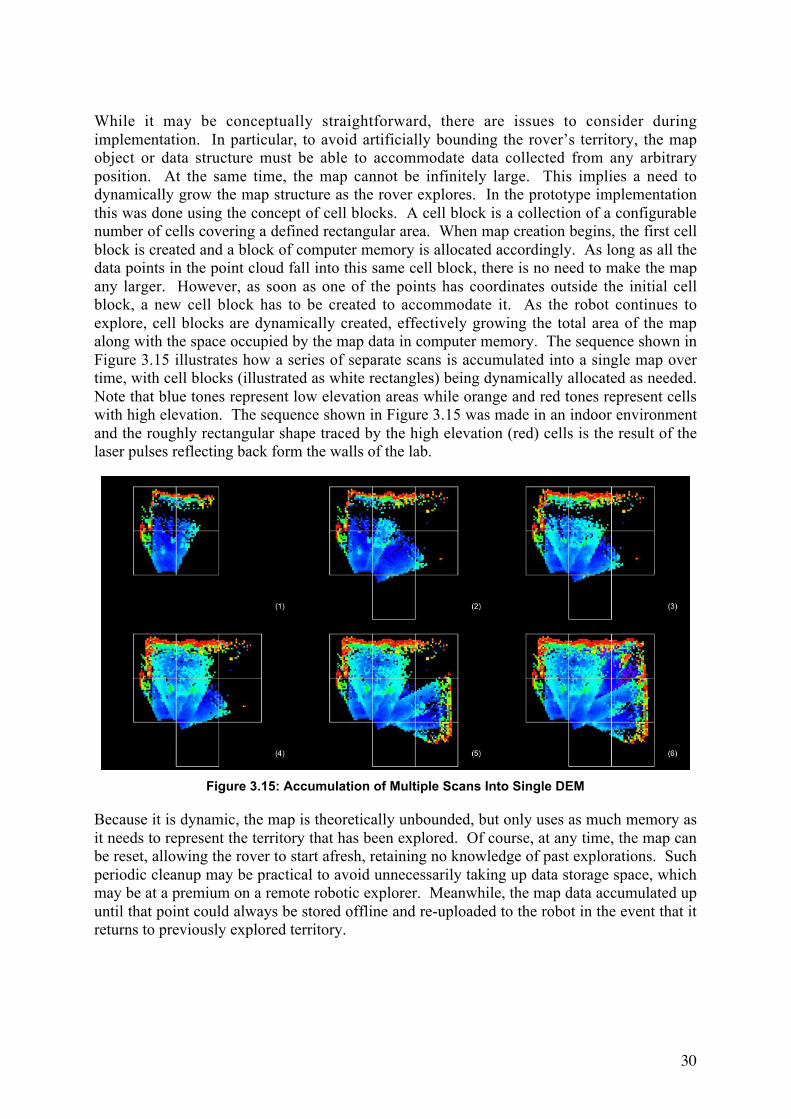
30
While it may be conceptually straightforward, there are issues to consider during
implementation. In particular, to avoid artificially bounding the rover’s territory, the map
object or data structure must be able to accommodate data collected from any arbitrary
position. At the same time, the map cannot be infinitely large. This implies a need to
dynamically grow the map structure as the rover explores. In the prototype implementation
this was done using the concept of cell blocks. A cell block is a collection of a configurable
number of cells covering a defined rectangular area. When map creation begins, the first cell
block is created and a block of computer memory is allocated accordingly. As long as all the
data points in the point cloud fall into this same cell block, there is no need to make the map
any larger. However, as soon as one of the points has coordinates outside the initial cell
block, a new cell block has to be created to accommodate it. As the robot continues to
explore, cell blocks are dynamically created, effectively growing the total area of the map
along with the space occupied by the map data in computer memory. The sequence shown in
Figure 3.15 illustrates how a series of separate scans is accumulated into a single map over
time, with cell blocks (illustrated as white rectangles) being dynamically allocated as needed.
Note that blue tones represent low elevation areas while orange and red tones represent cells
with high elevation. The sequence shown in Figure 3.15 was made in an indoor environment
and the roughly rectangular shape traced by the high elevation (red) cells is the result of the
laser pulses reflecting back form the walls of the lab.
Figure 3.15: Accumulation of Multiple Scans Into Single DEM
Because it is dynamic, the map is theoretically unbounded, but only uses as much memory as
it needs to represent the territory that has been explored. Of course, at any time, the map can
be reset, allowing the rover to start afresh, retaining no knowledge of past explorations. Such
periodic cleanup may be practical to avoid unnecessarily taking up data storage space, which
may be at a premium on a remote robotic explorer. Meanwhile, the map data accumulated up
until that point could always be stored offline and re-uploaded to the robot in the event that it
returns to previously explored territory.
31
3.3 Terrain Assessment and Costing
In the context of the work discussed here, costing refers to assigning a measure of the
assessed difficulty of having the rover traverse a given piece of terrain. The most obvious
factors to consider are the roughness, steepness or stability of the terrain but in some cases,
other factors such as access to sunlight or line-of-sight with communications antennas could
be important. In any case, the purpose of costing is to influence the path planning algorithms
to keep the rover away from trouble areas where it might have difficulties in physically
negotiating the terrain, maintaining adequate power via its solar arrays, or maintaining radio
contact, for example.
3.3.1 Potential Approaches
The costing function may be designed to help the path planning algorithm find path solutions
that are not only possible but are also optimal in that they avoid the unnecessary extra power
consumption resulting from having the rover navigate very steep slopes when a flatter route is
available. A sophisticated costing function could balance a large set of factors producing a
richly detailed cost map that could help optimize rover performance.
A more basic approach is for the costing function to produce a binary result where terrain that
can be traversed has zero cost and obstacles or non-traversable terrain have infinite cost. This
means that all traversable terrain is treated equally by path planning algorithms. In regions
where slopes are steep and terrain roughness is highly variable, this may lead to sub-optimal
paths but will at least keep the rover away from problem areas.
A hybrid approach might assign a range of costs to most parts of the terrain and infinite cost
to obstacles. The path-planning algorithm will look at the total cost of all the cells in the
robot’s footprint. If even one cell in the footprint has the impossibly high cost of an obstacle,
the corresponding robot position cannot be considered, even if the rest of the footprint gives a
very low cost. This prevents the robot from traversing through what seems to be a very
attractive, low-cost piece of terrain that contains an obstacle.
3.3.2 Solution for the Prototype Implementation
In the prototype implementation, several methods were attempted. At first, the only data
stored in each cell of the map was the maximum elevation. Terrain slopes were computed by
comparing the cell’s maximum elevation with that of each of four neighbouring cells.
Obstacles would cause steep slopes to appear in the map and these areas could be assigned
high costs to keep the path planner away. In practice, however, this method did not yield
good results. The DEM was then augmented to store not only the maximum, but also the
minimum elevation for each cell. The idea is that any cell that contains points spanning a
large vertical range must also have steep slopes within it. This method has the added
advantage of being computationally simpler since no neighbour cells need to be examined in
calculating the cost. Results were immediately promising but still not ideal. The parameter
defining the cost limit had to be found by trial and error and it proved difficult to find a value
that successfully identified true obstacles without also giving false positives.

32
A visual look at the point cloud leads to another idea. As seen in the point cloud, nearby
obstacles tend to have a large number of data points owing to the fact that they stick up from
the terrain and have surfaces nearly perpendicular to the sensor’s line of sight (see Figure
3.16). In other words, large numbers of data points are clustered together on the near side of
nearby obstacles. To test whether this was indeed a useful criterion for the identification of
obstacles, the DEM was again augmented to track the total number of points that are
accumulated into each cell when the data is reduced from the point cloud. The cost function
was redefined to use a combination of vertical range and number of data points for each cell.
After some parameter tuning, this method proved to be highly effective, assigning low cost to
flat terrain, higher cost to objects that protrude up from the generally flat terrain and giving
infinite cost to objects exceeding a certain threshold. Although results have been generally
good, there are some serious limitations to this approach. These issues and their possible
remedies are discussed in chapter 4.
X (meters)
Point Cloud
Ele
va
tio
n (
me
ters
)
-Y (meters)
Obstacles
Obstacle
Shadows
Figure 3.16: Point Cloud with Data Points Clustered on Obstacles
3.4 Path Planning
Generally, the goal of path planning is to find an efficient route for the robot to follow to get
from one point to another without having to traverse terrain that is difficult, dangerous or
impossible to negotiate. Typically, this is done as a graph-search problem wherein the nodes
in the graph represent potential robot positions and the edges represent connecting routes
between those points. In a grid-based map, each cell would be a node and the edges represent
movement between adjacent cells. Costs are assigned to either the nodes or the edges in the
graph based on characteristics such as local roughness or steepness of the terrain. The goal is
to find an efficient path that avoids impossibly high-cost terrain (i.e. obstacles).
33
3.4.1 Potential Approaches
The classic solution to finding the best path through a graph is Dijkstra’s algorithm, first
published in 1959. This algorithm measures the cost (sometimes simply the distance) of
travelling between each node of the graph and then computes a total cost for every possible
route from a specified starting point to every other point. The algorithm is widely used in
computer networking to find the optimal routing for sending TCP/IP packets between two
distant computers. The algorithm could be applied to the rover path-planning problem except
that because it is exhaustive, it is impractical for robots that have a large number of possible
routes to get to their destination. In a dense grid-based map, the number of nodes and edges
in the graph would be very large making this approach prohibitively expensive in terms of
computational power.
Instead, the traditional algorithm applied to vehicle path planning is A*, pronounced “A star”.
This algorithm is a best-first search that can converge to an optimal solution without having to
check every possible path exhaustively. For traversing a given node in the graph, the
algorithm estimates the total cost as the accumulated cost from the start to the current node
(usually called g(x)) plus an estimate of the remaining cost to get to the destination (usually
called h(x)). The accumulated cost so far, g(x), is measured along the way and is therefore
known precisely. On the other hand, the estimated remaining cost, h(x), is merely a heuristic
best-case scenario estimate. At each step, the “current node” advances towards whichever of
its neighbours appears, based on the estimated remaining cost, to be the most promising route
towards the goal. This is the concept of a best-first search. Since the estimate, h(x), is
optimistic, a route with a high estimated total cost is guaranteed to cost at least as much as the
estimate, so it need not be investigated as long as there exist other options that appear to be
less costly. A given route continues to be investigated until it no longer appears to be the best
possible option. Hence, at all times, the algorithm pursues the best possible option until
finally the goal is reached. Since the option being explored at this point is already the best of
the possible choices, the A* algorithm guarantees a globally optimal solution.
For exploration rovers, knowledge of the environment is initially incomplete but generally
improves with time. Since the A* algorithm is complex and computationally intensive, it
would be inefficient to have to repeat the algorithm from the start every time the robot gathers
new information about its environment. Stentz (1994) therefore developed D* (“D star”),
which is a dynamic version of the A* algorithm that works in reverse and avoids having to
update the entire path when new information becomes available.
Another approach is to use the concept of Potential Fields (PFs), which effectively push the
robot towards the goal. This concept can be visualized as placing a positive charge at the
starting point and a negative charge at the goal, causing electric potential to flow from the
start to the goal. The robot is then represented as a free-floating positive charge that is
repelled by the starting point and attracted towards the goal. Obstacles are also given positive
charges causing the robot to avoid them. The concept is appealing and can be successful but
can also end up trapped in local minima.
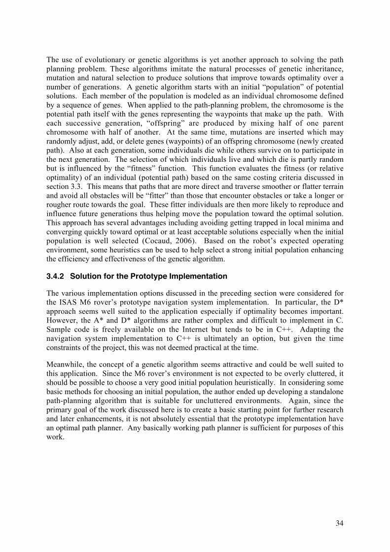
34
The use of evolutionary or genetic algorithms is yet another approach to solving the path
planning problem. These algorithms imitate the natural processes of genetic inheritance,
mutation and natural selection to produce solutions that improve towards optimality over a
number of generations. A genetic algorithm starts with an initial “population” of potential
solutions. Each member of the population is modeled as an individual chromosome defined
by a sequence of genes. When applied to the path-planning problem, the chromosome is the
potential path itself with the genes representing the waypoints that make up the path. With
each successive generation, “offspring” are produced by mixing half of one parent
chromosome with half of another. At the same time, mutations are inserted which may
randomly adjust, add, or delete genes (waypoints) of an offspring chromosome (newly created
path). Also at each generation, some individuals die while others survive on to participate in
the next generation. The selection of which individuals live and which die is partly random
but is influenced by the “fitness” function. This function evaluates the fitness (or relative
optimality) of an individual (potential path) based on the same costing criteria discussed in
section 3.3. This means that paths that are more direct and traverse smoother or flatter terrain
and avoid all obstacles will be “fitter” than those that encounter obstacles or take a longer or
rougher route towards the goal. These fitter individuals are then more likely to reproduce and
influence future generations thus helping move the population toward the optimal solution.
This approach has several advantages including avoiding getting trapped in local minima and
converging quickly toward optimal or at least acceptable solutions especially when the initial
population is well selected (Cocaud, 2006). Based on the robot’s expected operating
environment, some heuristics can be used to help select a strong initial population enhancing
the efficiency and effectiveness of the genetic algorithm.
3.4.2 Solution for the Prototype Implementation
The various implementation options discussed in the preceding section were considered for
the ISAS M6 rover’s prototype navigation system implementation. In particular, the D*
approach seems well suited to the application especially if optimality becomes important.
However, the A* and D* algorithms are rather complex and difficult to implement in C.
Sample code is freely available on the Internet but tends to be in C++. Adapting the
navigation system implementation to C++ is ultimately an option, but given the time
constraints of the project, this was not deemed practical at the time.
Meanwhile, the concept of a genetic algorithm seems attractive and could be well suited to
this application. Since the M6 rover’s environment is not expected to be overly cluttered, it
should be possible to choose a very good initial population heuristically. In considering some
basic methods for choosing an initial population, the author ended up developing a standalone
path-planning algorithm that is suitable for uncluttered environments. Again, since the
primary goal of the work discussed here is to create a basic starting point for further research
and later enhancements, it is not absolutely essential that the prototype implementation have
an optimal path planner. Any basically working path planner is sufficient for purposes of this
work.

35
The concept of the author’s path planning algorithm starts from the assumption that the
rover’s environment is relatively uncluttered. Indeed, there is a high probability that a safe
straight-line path connects the starting point with the goal. Figure 3.17 illustrates this
situation showing obstacles in red, the initial and final footprints of the rover in blue and
green, respectively, the path itself as a solid, arrowed line and the area swept out by the
rover’s footprint bounded by dashed lines. Here, there is no need for any computation beyond
a quick check verifying that the assumed swath is in fact clear of obstacles.
Figure 3.17: Initially-Assumed Path is Already Clear
If, instead of being completely clear, the path contains some obstacles, the algorithm’s
starting assumption of a clear path will turn out to be false (see Figure 3.18).
Figure 3.18: Initially-Assumed Path is Not Clear
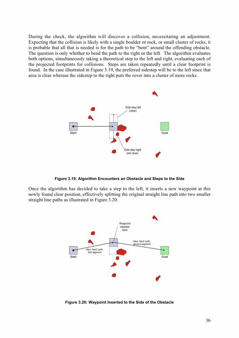
36
During the check, the algorithm will discover a collision, necessitating an adjustment.
Expecting that the collision is likely with a single boulder or rock, or small cluster of rocks, it
is probable that all that is needed is for the path to be “bent” around the offending obstacle.
The question is only whether to bend the path to the right or the left. The algorithm evaluates
both options, simultaneously taking a theoretical step to the left and right, evaluating each of
the projected footprints for collisions. Steps are taken repeatedly until a clear footprint is
found. In the case illustrated in Figure 3.19, the preferred sidestep will be to the left since that
area is clear whereas the sidestep to the right puts the rover into a cluster of more rocks.
Figure 3.19: Algorithm Encounters an Obstacle and Steps to the Side
Once the algorithm has decided to take a step to the left, it inserts a new waypoint at this
newly found clear position, effectively splitting the original straight line path into two smaller
straight line paths as illustrated in Figure 3.20.
Figure 3.20: Waypoint Inserted to the Side of the Obstacle
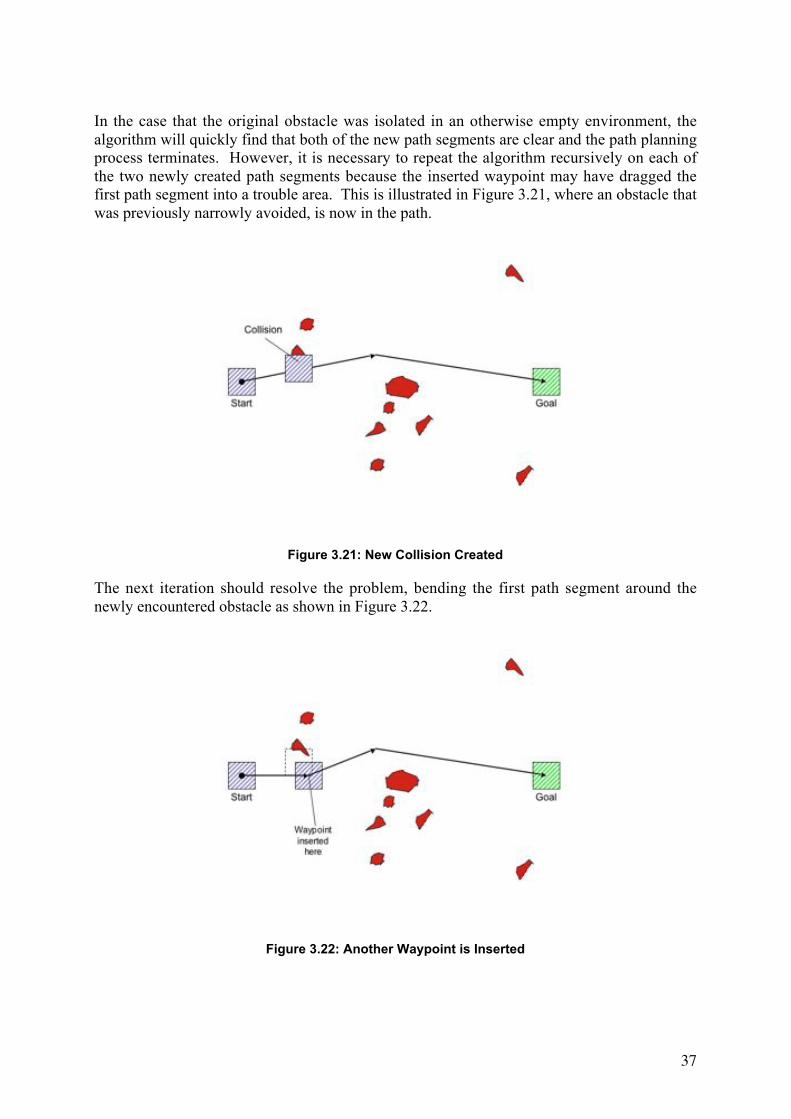
37
In the case that the original obstacle was isolated in an otherwise empty environment, the
algorithm will quickly find that both of the new path segments are clear and the path planning
process terminates. However, it is necessary to repeat the algorithm recursively on each of
the two newly created path segments because the inserted waypoint may have dragged the
first path segment into a trouble area. This is illustrated in Figure 3.21, where an obstacle that
was previously narrowly avoided, is now in the path.
Figure 3.21: New Collision Created
The next iteration should resolve the problem, bending the first path segment around the
newly encountered obstacle as shown in Figure 3.22.
Figure 3.22: Another Waypoint is Inserted

38
When all path segments are clear of obstacles, the algorithm terminates leaving an acceptable
solution to the path-planning problem as illustrated in Figure 3.23. Again, note that it is not
only the path line itself that must avoid obstacles but the entire swath of the robot’s footprint
as it follows that path.
Figure 3.23: Final Path is Clear of All Obstacles
The illustrated example is, of course, oversimplified. In practice, a larger number of smaller
sidesteps is typically taken when circumnavigating an obstacle. This results in several
waypoints being clustered together on the near side of an obstacle as illustrated in Figure
3.24, which is an experimental result. In this illustration, blue areas represent traversable
terrain while red areas represent obstacles; the destination is in an unexplored area (black) to
the right of the picture.
Figure 3.24: Path Planning Algorithm Result Before Simplification
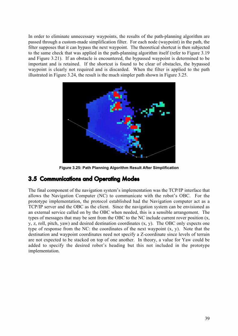
39
In order to eliminate unnecessary waypoints, the results of the path-planning algorithm are
passed through a custom-made simplification filter. For each node (waypoint) in the path, the
filter supposes that it can bypass the next waypoint. The theoretical shortcut is then subjected
to the same check that was applied in the path-planning algorithm itself (refer to Figure 3.19
and Figure 3.21). If an obstacle is encountered, the bypassed waypoint is determined to be
important and is retained. If the shortcut is found to be clear of obstacles, the bypassed
waypoint is clearly not required and is discarded. When the filter is applied to the path
illustrated in Figure 3.24, the result is the much simpler path shown in Figure 3.25.
Figure 3.25: Path Planning Algorithm Result After Simplification
3.5 Communications and Operating Modes
The final component of the navigation system’s implementation was the TCP/IP interface that
allows the Navigation Computer (NC) to communicate with the robot’s OBC. For the
prototype implementation, the protocol established had the Navigation computer act as a
TCP/IP server and the OBC as the client. Since the navigation system can be envisioned as
an external service called on by the OBC when needed, this is a sensible arrangement. The
types of messages that may be sent from the OBC to the NC include current rover position (x,
y, z, roll, pitch, yaw) and desired destination coordinates (x, y). The OBC only expects one
type of response from the NC: the coordinates of the next waypoint (x, y). Note that the
destination and waypoint coordinates need not specify a Z-coordinate since levels of terrain
are not expected to be stacked on top of one another. In theory, a value for Yaw could be
added to specify the desired robot’s heading but this not included in the prototype
implementation.
40
Once started up and initialized, the navigation system is put into “Go to position” mode. Its
first task in this mode is to configure the TCP/IP socket and wait for a connection. When the
OBC is ready to start commanding the rover and requesting navigation information, it opens a
connection with the NC and the process begins. From the perspective of the navigation
system, the navigation service is provided on an on-demand basis. Thus, all its actions are
driven by requests or “commands” it receives from the client OBC. At any time, the OBC
may send a message updating the navigation system’s knowledge of the rover position or the
destination coordinates. The navigation system waits until each of these two messages has
been received at least once. Once both pieces of information are available, LIDAR scan data
is collected, processed and built into a world model, then a path is planned toward the
specified destination. Having determined a path, the navigation system sends a message back
to the OBC specifying the coordinates of the next waypoint. At this point, execution stops
and waits for either of the two inputs to change (since there is no point in re-calculating a path
if the rover is not moving and the destination is unchanging). When the OBC sends an update
of either of these two inputs, the process is repeated beginning with a LIDAR scan and ending
with a response giving the next waypoint.
This is the nominal mode of operations and, once again, assumes that the OBC is capable of
estimating the rover’s position. If that is not possible, other modes of operation may be
required. Accordingly, and to support testing anyway, several other operational modes were
built into the navigation system application. These include diagnostics modes, single-scan
modes, and modes that only perform part of the sequence. Partial sequence modes include: a
scan-only mode that saves the scan results to a file for later processing; a mode that only
builds a map from a scan data file and saves the resulting map data; a mode that reads a map
data file, plans a path to user-specified coordinates and saves the path to a file; as well as
several combination modes. Due to the modularity of the various required functions, new
operation modes can be generated with relative ease. The impromptu mode creation
described in section 4.1.5 is an example of how this can be very practical.
41
4 Discussion and Future Work
This chapter takes a critical look at the implemented navigation system in light of
experimental results from both the laboratory and field trials. Generally, the system delivers
satisfactory results but there are some issues that beg further study. The chapter ends with a
look at potential development towards a broader implementation of robot autonomy.
4.1 Experimental Results
Because the goal was only to establish a starting point for an end-to-end navigation system,
development stopped once satisfactory results were obtained. No systematic testing
campaign has yet been undertaken to reveal potential flaws. Nevertheless, in the course of
developing and debugging the system, a number of experiments were conducted both in the
lab and in the field with varying, yet generally good results.
4.1.1 Laser Range Finder (LRF) Results
One of the first challenges in dealing with the LRF was in understanding the timing of the
data collection. When it is first powered up, a considerable warm-up time is required before
the scan results begin to become useful. Scan data collected in the first minute or so tend to
suffer from a large amount of random noise. Also, the device does not perform scans on
demand but instead scans continually. Once data is requested from the device, the buffer is
emptied and then replaced with the latest data. This means that to get a scan of the current
field of view, two requests are actually required: one to clear out the stale data from the buffer
and another to collect the new data.
Another problem discussed previously is that the cleanliness of the lens has a major influence
on performance. Even so much as a fingerprint on the lens can cause problems. Observations
suggest that when viewing distant or poorly reflecting features through a dirty or smudged
lens, distance is often estimated to be near zero, if not negative. Curiously, under identical
lens conditions, when brightly reflecting objects are placed in the field of view, they are
measured accurately. Clearly, the lens must be kept clean to avoid these problems.
As expected, lighting conditions were found to have no effect on the LIDAR performance.
Performance of the LRF appeared to be the same in the office, in the laboratory, and outside
both in cloudy and sunny conditions. This confirms that LIDAR operates consistently
through a range of lighting conditions and can therefore be an asset in complementing stereo
vision data.
42
The varying laser reflectivity of different surfaces can be an issue. Some types of rocks
reflect more strongly than others. The problem is that when the reflection is weak, the
distance estimate tends to be noisier. Within 2-3 meters of the sensor, most surfaces produce
a fairly strong reflection and distance estimates tend to be good. In the laboratory, return
signals are received from surfaces as far away as the walls, up to some 9 meters away from
the sensor, but for anything beyond a few meters, moderate noise exists in the distance
estimates. In outdoor trials, on level terrain, return signals are received from the terrain at up
to about 6 meters from the sensor. The fact that more distant measurements were observed on
indoor trials is due to the fact that the walls stand nearly perpendicular to the sensor’s line of
sight. Naturally, this near 90º angle of incidence results in strong reflections while the
oblique angle the sensor makes with the ground plane, usually 15º or 30º, results in weaker
reflections and no returning laser pulses from terrain beyond about 6 meters from the sensor.
When the laser pulse does not return to the sensor at all, the reflectivity value is recorded as
zero and the distance estimate leaps to the value of 14.6 meters indicating an invalid
measurement that will be filtered out (see section 3.1.2).
Again, since there was no extensive characterization campaign, the only ground-plane
surfaces that were observed were those of the testing areas: the tiled office floor, the sand in
the laboratory, and the grass in the outdoor field. None of these surfaces proved to be
problematic and within the near range of the sensor, distance estimates seemed to be
reasonably good for all of these surfaces. Note that some of the outdoor trials were conducted
shortly after rainfall meaning that the grass was damp. Although this was initially a concern
for the LIDAR performance, it proved to be a non-issue. Performance even on the damp
grass was satisfactory. Since further field-testing was not conducted, however, it is not clear
whether performance on dry grass might be even better.
4.1.2 Modelling Results
As outlined in section 3.2, modelling begins with converting the sensor measurements into
Cartesian coordinates and transforming the data into a consistent frame of reference. This
requires knowledge of the sensor’s pose with respect to that universal frame of reference.
Failing that, at least the attitude of the sensor must be known in order to produce accurate
local models.
At this time, the mast on which the sensor is mounted on the M6 rover is not motorized or
controlled in any way. This will be implemented eventually in order to allow the robot to
survey its surroundings from a fixed position, but for now, the sensor is fixed on the mast.
The angle the sensor’s line of sight makes with the horizontal can be adjusted mechanically
but not in any precise way. This leads to slight errors in the estimated pose of the sensor
relative to the robot. Furthermore, the robot’s precise attitude is not currently known and is
therefore assumed to be flat for simplicity. This contributes to even more error in the
estimated pose of the sensor with respect to the ground plane. This means that a ground plane
may appear to be slightly inclined in the model even if it is, in fact, perfectly level. Naturally,
this will lead to errors in elevation estimates and could ultimately impact the path planning
performance. Some of the laboratory testing also saw the sensor mounted on a tripod rather
than on the robot itself. Since the tripod’s feet can be placed at varying depths into the sand,
and since no precise leveling tool is currently in place, this leads to similar errors.
43
As discussed under the assumptions of section 2.3.2, the lack of knowledge of the robot’s
position in an absolute frame of reference has a major impact on modelling. Without this
knowledge, the robot can still model the immediate environment with respect to its own body
frame but multiple measurements cannot be combined into a single map. This, in fact, has
become the case since the M6 rover so far is not able to estimate its own position in an
absolute frame of reference. Until this is implemented, the navigation system can only be
operated in single-scan mode, modelling only what it can see at a given moment, and
necessarily resetting its map on each cycle, therefore not accumulating environmental
knowledge over time.
A separate issue encountered during modelling is the occasional erroneous appearance of
vertical columns in the model. This occurs in indoor environments when a scan collects data
points both on the ground plane as well as from the ceiling. Since, technically, the affected
cell has data at both extremes, it supposes they are connected and that a column exists at that
location, even when there is none. This highlights a previously unrecognized implicit
assumption that all observed points in the robot’s environment are parts of objects rising up
from the ground plane. While this assumption fails in the laboratory, it is reasonable for a
lunar or planetary surface prior to the construction of any artificial structures. Hence, this is
not considered a serious problem at the moment. To avoid the problem in the laboratory,
another assumption was introduced: it is now assumed that objects above the plane of the
sensor are not relevant to the robot since it can never reach them without first encountering
some rising terrain anyway.
4.1.3 Costing Results
As presented in section 3.3.2, the terrain assessment and costing system put in place for the
prototype implementation makes use of just two pieces of information stored in each cell of
the DEM: the vertical range of data points for that cell (an indication of terrain steepness in
the cell) and the number of data points (an indication of how perpendicular the surfaces are to
the sensor’s line of sight – obstacles tend to have this attribute).
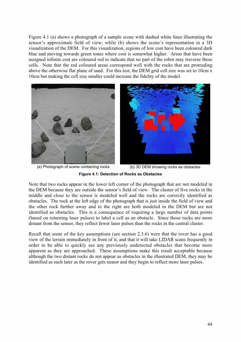
44
Figure 4.1 (a) shows a photograph of a sample scene with dashed white lines illustrating the
sensor’s approximate field of view; while (b) shows the scene’s representation in a 3D
visualization of the DEM. For this visualization, regions of low cost have been coloured dark
blue and moving towards green tones where cost is somewhat higher. Areas that have been
assigned infinite cost are coloured red to indicate that no part of the robot may traverse these
cells. Note that the red coloured areas correspond well with the rocks that are protruding
above the otherwise flat plane of sand. For this test, the DEM grid cell size was set to 10cm x
10cm but making the cell size smaller could increase the fidelity of the model.
(a) Photograph of scene containing rocks (b) 3D DEM showing rocks as obstacles
Figure 4.1: Detection of Rocks as Obstacles
Note that two rocks appear in the lower left corner of the photograph that are not modeled in
the DEM because they are outside the sensor’s field of view. The cluster of five rocks in the
middle and close to the sensor is modeled well and the rocks are correctly identified as
obstacles. The rock at the left edge of the photograph that is just inside the field of view and
the other rock further away and to the right are both modeled in the DEM but are not
identified as obstacles. This is a consequence of requiring a large number of data points
(based on returning laser pulses) to label a cell as an obstacle. Since those rocks are more
distant from the sensor, they reflect fewer laser pulses than the rocks in the central cluster.
Recall that some of the key assumptions (see section 2.3.6) were that the rover has a good
view of the terrain immediately in front of it, and that it will take LIDAR scans frequently in
order to be able to quickly see any previously undetected obstacles that become more
apparent as they are approached. These assumptions make this result acceptable because
although the two distant rocks do not appear as obstacles in the illustrated DEM, they may be
identified as such later as the rover gets nearer and they begin to reflect more laser pulses.
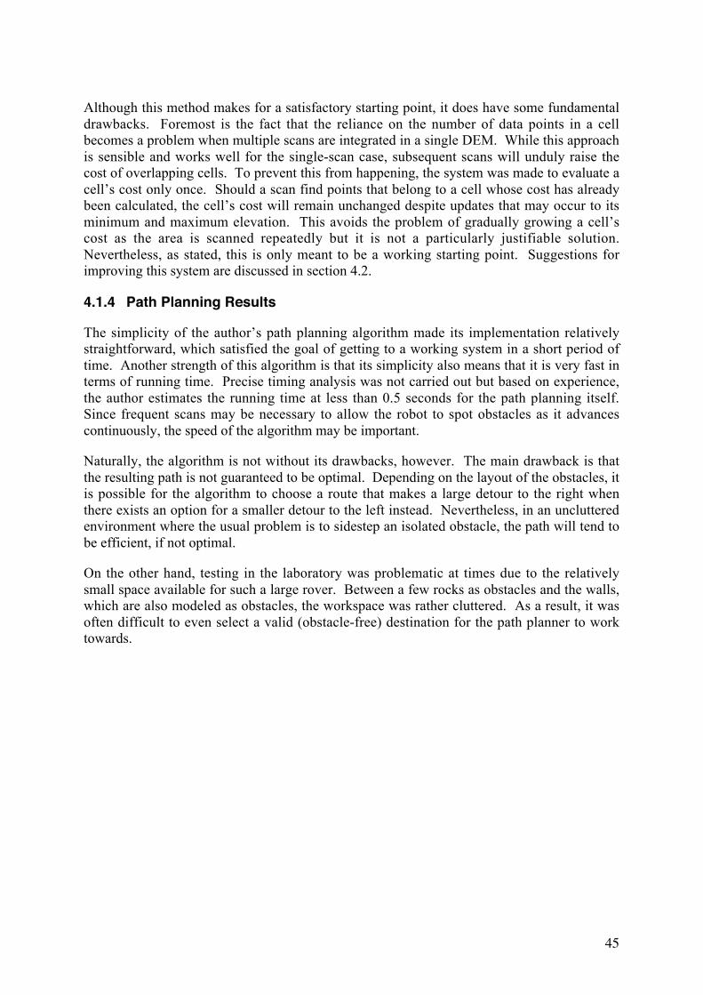
45
Although this method makes for a satisfactory starting point, it does have some fundamental
drawbacks. Foremost is the fact that the reliance on the number of data points in a cell
becomes a problem when multiple scans are integrated in a single DEM. While this approach
is sensible and works well for the single-scan case, subsequent scans will unduly raise the
cost of overlapping cells. To prevent this from happening, the system was made to evaluate a
cell’s cost only once. Should a scan find points that belong to a cell whose cost has already
been calculated, the cell’s cost will remain unchanged despite updates that may occur to its
minimum and maximum elevation. This avoids the problem of gradually growing a cell’s
cost as the area is scanned repeatedly but it is not a particularly justifiable solution.
Nevertheless, as stated, this is only meant to be a working starting point. Suggestions for
improving this system are discussed in section 4.2.
4.1.4 Path Planning Results
The simplicity of the author’s path planning algorithm made its implementation relatively
straightforward, which satisfied the goal of getting to a working system in a short period of
time. Another strength of this algorithm is that its simplicity also means that it is very fast in
terms of running time. Precise timing analysis was not carried out but based on experience,
the author estimates the running time at less than 0.5 seconds for the path planning itself.
Since frequent scans may be necessary to allow the robot to spot obstacles as it advances
continuously, the speed of the algorithm may be important.
Naturally, the algorithm is not without its drawbacks, however. The main drawback is that
the resulting path is not guaranteed to be optimal. Depending on the layout of the obstacles, it
is possible for the algorithm to choose a route that makes a large detour to the right when
there exists an option for a smaller detour to the left instead. Nevertheless, in an uncluttered
environment where the usual problem is to sidestep an isolated obstacle, the path will tend to
be efficient, if not optimal.
On the other hand, testing in the laboratory was problematic at times due to the relatively
small space available for such a large rover. Between a few rocks as obstacles and the walls,
which are also modeled as obstacles, the workspace was rather cluttered. As a result, it was
often difficult to even select a valid (obstacle-free) destination for the path planner to work
towards.
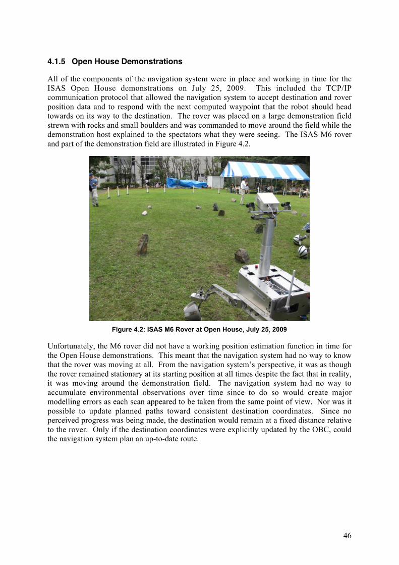
46
4.1.5 Open House Demonstrations
All of the components of the navigation system were in place and working in time for the
ISAS Open House demonstrations on July 25, 2009. This included the TCP/IP
communication protocol that allowed the navigation system to accept destination and rover
position data and to respond with the next computed waypoint that the robot should head
towards on its way to the destination. The rover was placed on a large demonstration field
strewn with rocks and small boulders and was commanded to move around the field while the
demonstration host explained to the spectators what they were seeing. The ISAS M6 rover
and part of the demonstration field are illustrated in Figure 4.2.
Figure 4.2: ISAS M6 Rover at Open House, July 25, 2009
Unfortunately, the M6 rover did not have a working position estimation function in time for
the Open House demonstrations. This meant that the navigation system had no way to know
that the rover was moving at all. From the navigation system’s perspective, it was as though
the rover remained stationary at its starting position at all times despite the fact that in reality,
it was moving around the demonstration field. The navigation system had no way to
accumulate environmental observations over time since to do so would create major
modelling errors as each scan appeared to be taken from the same point of view. Nor was it
possible to update planned paths toward consistent destination coordinates. Since no
perceived progress was being made, the destination would remain at a fixed distance relative
to the rover. Only if the destination coordinates were explicitly updated by the OBC, could
the navigation system plan an up-to-date route.
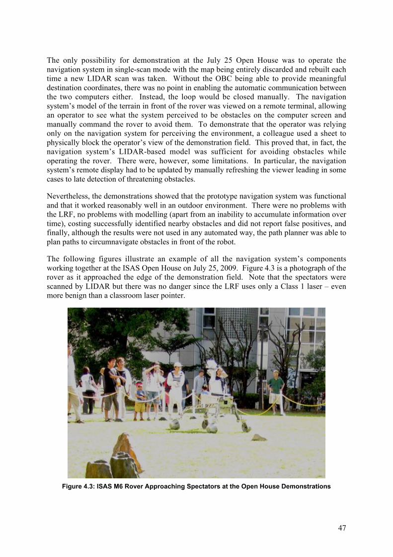
47
The only possibility for demonstration at the July 25 Open House was to operate the
navigation system in single-scan mode with the map being entirely discarded and rebuilt each
time a new LIDAR scan was taken. Without the OBC being able to provide meaningful
destination coordinates, there was no point in enabling the automatic communication between
the two computers either. Instead, the loop would be closed manually. The navigation
system’s model of the terrain in front of the rover was viewed on a remote terminal, allowing
an operator to see what the system perceived to be obstacles on the computer screen and
manually command the rover to avoid them. To demonstrate that the operator was relying
only on the navigation system for perceiving the environment, a colleague used a sheet to
physically block the operator’s view of the demonstration field. This proved that, in fact, the
navigation system’s LIDAR-based model was sufficient for avoiding obstacles while
operating the rover. There were, however, some limitations. In particular, the navigation
system’s remote display had to be updated by manually refreshing the viewer leading in some
cases to late detection of threatening obstacles.
Nevertheless, the demonstrations showed that the prototype navigation system was functional
and that it worked reasonably well in an outdoor environment. There were no problems with
the LRF, no problems with modelling (apart from an inability to accumulate information over
time), costing successfully identified nearby obstacles and did not report false positives, and
finally, although the results were not used in any automated way, the path planner was able to
plan paths to circumnavigate obstacles in front of the robot.
The following figures illustrate an example of all the navigation system’s components
working together at the ISAS Open House on July 25, 2009. Figure 4.3 is a photograph of the
rover as it approached the edge of the demonstration field. Note that the spectators were
scanned by LIDAR but there was no danger since the LRF uses only a Class 1 laser – even
more benign than a classroom laser pointer.
Figure 4.3: ISAS M6 Rover Approaching Spectators at the Open House Demonstrations

48
Figure 4.4 shows a LIDAR scan taken at approximately the same time as the photograph
shown above. Several spectators are clearly discernable about 3 meters from the sensor while
portions of others at greater distances, around 5-6 meters, can be made out just at the limit of
the sensor’s practical range.
Figure 4.4: LIDAR Scan of Spectators at the Edge of the Demonstration Field
Once converted to a point cloud and then collapsed into a DEM, the scene is modeled as a
series of 10 cm x 10 cm vertical columns as shown in Figure 4.5. In this visualization, the
colours represent maximum elevation in each cell with higher elevation indicated by red
tones, then moving through orange, yellow, green and finally blue tones for the lowest
elevation cells.
Figure 4.5: 3D DEM Modelling Spectators with Vertical Columns

49
Costing was then done on the cells in the DEM to identify which cells represent definite
obstacles and must therefore be avoided. Figure 4.6 shows 2D and 3D visualizations of the
DEM with low cost cells in dark blue tones, lighter blue and aqua tones for higher cost cells,
and red for cells that have been identified as obstacles. As expected, each of the nearby
spectators is identified as an obstacle.
Figure 4.6: 2D and 3D DEM Identifying Obstacles (shown in red)
Finally, having modeled the space before the rover and identified obstacles within it, an
obstacle-avoiding path could be planned. Again, there was no way for the path planner to
keep track of a meaningful destination as the rover moved around, but as a demonstration of
the path planner’s capabilities, a path was planned for every completed LIDAR scan (about
once every 2 seconds). The destination was set arbitrarily at 10 meters straight ahead of the
rover. Whenever the rover was attempting to drive straight ahead, the resulting path would
actually be useful. Otherwise, it just gave a rough guide as to whether to go left or right to
avoid obstacles. Figure 4.7 shows the results of a simplified path that circumnavigates all
known obstacles (in this case, the spectators within the sensor’s field of view) and puts the
rover on a course toward its arbitrary destination, 10 meters straight ahead.
Figure 4.7: Obstacle-Avoiding Path Planned Around Spectators
50
4.2 Proposed System Improvements
Although the results obtained so far have been generally satisfactory, and certainly make for a
useful starting point, there is a great deal of room for improvement. This section outlines a
number of improvements that could be made to the navigation system.
4.2.1 Programming Language
One of the first things that should be done is to port the implementation from C to C++. The
work was started in C and it did not become clear until well into the project that a C++
implementation may also be acceptable for the on-board computer. The author opted to first
complete the prototype implementation in C but hoped to move it to C++ at a later time since
the more powerful language is much better suited to the concepts applied in the
implementation.
In an effort to be modular, the system makes use of a number of object-like structures that
could be much better handled in object-oriented C++. A programmer who may be interested
in continuing this work will see that the current implementation includes functions that should
be implemented as object methods working with member variables. Instead, the current
solution is to have the calling functions pass an object handle (in fact, just a structure
pointer’s address for now) in order to give the function access to the object’s variables. This
also means that create and destroy functions are necessary to manage the memory allocations
associated with these quasi-objects. All of this is rather cumbersome and prone to error.
Most errors are caught by extensive error checking but the practice of manually managing
memory is dangerous and some critical bugs are likely to be found with more extensive
testing.
Moving to C++ will not only help avoid problems with the current implementation but will
also improve modularity and make the system more friendly for researchers who may wish to
work with the system to modify or replace its components.
4.2.2 Terrain Assessment and Costing
As stated previously, the choice of what information to store in the cells of the DEM depends
mainly on what information is needed for terrain analysis and costing. Currently, only the
minimum and maximum elevations are stored along with a counter recording how many point
cloud points were collapsed into the cell in question. Since the point count value does not
have direct physical meaning in terms of representing an object, and since its value can
change over time for the same object, it is fundamentally not a good parameter for the
identification of obstacles. Ideally, the costing function should use only parameters that are
physically meaningful. Over multiple successive scans, the value of a parameter that is
physically meaningful should converge, not grow monotonically as the point count does.
Examples of physically meaningful parameters include: maximum elevation, vertical range,
vertical standard deviation, and surface normal. The first two of these are sensible parameters
that are already stored in the current implementation.
51
Vertical standard deviation of the constituent points may provide a meaningful measure of the
roughness or steepness of the cell’s terrain. An obstacle should exhibit a wide range of
vertical points, spread evenly across that range therefore having a large vertical range and
large standard deviation. A piece of flat terrain plus an erroneous data point hovering high
above it will have a large vertical range, but a very low standard deviation, suggesting that it
is perhaps flatter than what is indicated by considering its vertical range alone. This could be
added relatively easily to the current implementation by storing a small point cloud object
within the cell object allowing the portion of the original cloud that belongs in a cell to remain
stored within that cell. Once the original point cloud is collected into the DEM, each cell’s
mini point cloud can be used to compute the vertical standard deviation of its points.
This same mini point cloud for a given cell could be used to estimate the mean slope in that
cell. If a plane is fitted to the cell’s mini point cloud, the normal to that plane gives an
indication of the slope in that cell. In flat terrain, the normal should be close to perpendicular
to the ground plane. Obstacles, on the other hand, may have surface normals nearly parallel
to the ground plane, indicating a steep slope.
Another area that may be worth studying is to start from the notion of the point count that is
used in the current implementation. While this number is not physically meaningful in itself,
it does yield good results for the single scan case and so it may be worth trying to derive a
physically meaningful value from it. It may also be worth considering resetting the point
count once the cost has been calculated. This way, the count could reflect only points
collected in the most recent scan. Some way to combine the previous cost with the cost
associated with the new points would have to be devised.
4.2.3 Point Tracking for Localization
As discussed in 4.1, the current system is severely limited in practice due to the fact that the
M6 rover is not yet able to compute its own position. Even if and when the robot is able to
estimate its position based on wheel odometery, this method is prone to rapid accumulation of
error, especially in terrain where wheel slippage is a problem.
Another option is to let the navigation system perform localization on its own. Vision-based
localization has become popular as it offers a significant improvement over wheel odometry,
estimating the robot’s position accurately with very little accumulation of error over time
(Matthies et al., 2007). As long as there is some overlap between successively viewed scenes,
points can be tracked from one cloud to the next producing an estimate of the amount of
motion of the camera. Stereo vision provides 3D information and thus allows this estimate to
be done in 3 dimensions. Since the point cloud data produced from the LIDAR scan gives
this same information, the same principle can be applied here.
Such a localization function could operate as a separate module that reads incoming point
cloud data (either from LIDAR data or stereo vision, or both) and feeds the results of its
position estimate to the world model module (the DEM). This localization module could also
accept as an input, the rover’s wheel odometry-based estimate in case it is somehow useful.
Since this module becomes an essential part of mapping, this is effectively Simultaneous
Localization and Mapping (SLAM).
52
To test the feasibility of this, a proof of concept was done using freely downloaded Matlab
code available from Mian (2009). The Matlab code takes two point clouds as inputs and
applies ICP (Iterative Closest Point) matching to estimate the distance that one cloud is
shifted from the other. A quick test was done in which the author manually shifted a point
cloud by a known amount and then passed both the unshifted and shifted clouds into the
Matlab routine to see if it could recover the transformation. The estimate was reasonably
close. Having demonstrated the possibility that this could work, the author conducted no
futher testing, however. Since the Matlab implementation made use of many built-in Matlab
librarires, porting the code to C or C++ could require a considerable amount of time. As
such, the author has chosen to leave this to future work.
4.2.4 Path Planning
The path planning algorithm presented here has been useful and generally successful in
uncluttered environments. Nevertheless, it is not very sophisticated and is prone to problems
when the robot’s workspace is more complex, such as in indoor spaces or where there is a
large distribution of obstacles.
A more sure solution is something traditional such as A* or better yet, its variant, D*, which
is more suitable for a robot that is moving around and gradually learning more about its
environment. Based on the work presented by Cocaud (2006), there is also reason to believe
that genetic algorithms may be suitable for the M6 rover. Of course, the navigation system
presented here should be equally suitable as a testbed for any number of other path planning
algorithms.
4.2.5 Stereo Vision
A relatively easy add-on to the current navigation system would be the integration of stereo
vision based models. A stereo vision system that produces point clouds can be integrated
seamlessly since the modelling component of the navigation system is not concerned with the
origin of the point cloud data, only its format. The model could collect point clouds from
stereo vision and LIDAR sources alike, integrating them into a single model. If for some
reason it is desirable to identify the source, a tag could easily be added to the point cloud
structure and to the mini point clouds within the cells of the DEM.
4.3 System Expansion
So far, future developments have been discussed specifically in the context of the navigation
and path planning system whose primary purpose is to help the rover avoid obstacles on its
way toward a specified destination. However, this says nothing about how such a destination
is selected.
Returning to the ideas discussed in section 1.2, the value of a robotic exploration vehicle can
be greatly enhanced by increasing its autonomy. The low-level autonomy of obstacle
avoidance is only the beginning; higher levels of autonomy to aid in task allocation,
prioritization, and managing of resources could greatly enhance scientific yield on exploration
missions.

53
Again, the M6 rover is a platform suitable for proving concepts of higher-level autonomy.
The work of Estlin, Castaño, and others at JPL, may provide a good example of the types of
intelligent decision-making that can be built into the M6 rover. To begin with, some overall
software architecture, such as the one described in 2.1.1 must be put in place to begin the
work of developing such higher levels of autonomy.
Ultimately, the M6 rover, as a testbed for rover technology in Japan, could reach levels of
autonomy well beyond simple path planning and obstacle avoidance. The rover could be used
to demonstrate autonomous decision-making that would allow: 1) a remote robotic explorer to
be highly productive by not requiring frequent consultations with Earth-based mission
controllers; and 2) a robot working in cooperation with human crews on the Moon or Mars or
elsewhere, to be flexible and responsive to the needs of their human colleagues.
54
5 Conclusions
The important matter of exploring the solar system relies to a large extent on the work of
mobile robots. In turn, the productivity and therefore value of these robots depends on their
ability to function without overly frequent guidance from Earth-based mission controllers.
Ideally, these robots should be able to balance priorities, manage their resources, and monitor
their own progress. But at a minimum, they should be able to handle minor problems such as
obstacle avoidance on their own.
The goal of the work described in this paper has been to develop a fully working, albeit basic,
autonomous navigation system to support future developments through field trials. The
intention has been to make the system modular enough to allow researchers to replace or
modify its components in order to test new and improved methods or to augment the system
by adding functionality. It is hoped that this system will serve as a starting point for
researchers who see the value of field trials as an effective means of advancing their work.
In the interest of completing the project in the short time available and considering that this
was only meant to be a starting point, the author tended to prefer simpler approaches at each
stage of the implementation. Nevertheless, the results of the prototype implementation are
generally good, especially in uncluttered outdoor environments.
The Laser Range Finder (LRF) was found to work equally well in any lighting conditions
both indoors and outside. On relatively level ground, the LRF data models the terrain well
over a radius of up to about 6 meters. The sensor data can be noisy and can include non-
credible measurements, especially when the lens is dirty, but a custom-designed filter
successfully removes these bad data points.
Based on the LRF data and the point cloud that results from its conversion to Cartesian
coordinates, the robot’s environment is modeled in a Cartesian-grid Digital Elevation Model
(DEM). This world model currently captures the vertical range of measurements in each of
its cells along with a count of the number of data points that have been collected into the cell.
In the current implementation, this is the only information used in terrain assessment.
Although results have been very good for the single-scan case, this approach to terrain
assessment does not lend itself well to the accumulation of data from multiple scans.
Concepts have been proposed for how to modify the terrain assessment method to consider
other, more physically meaningful parameters instead.
The path planning algorithm used in the prototype implementation is the author’s own and
has produced good results in relatively uncluttered spaces. Nevertheless, the algorithm may
be overly simplistic and, as such, may have limited robustness. Any of a number of other
methods outlined here could be implemented to replace the author’s basic algorithm. Note,
however, that as further sophistication is introduced, there is a risk that execution time may
grow.
55
At the ISAS Open House demonstrations on July 25, 2009, the end-to-end navigation system
was tested and found to work well. The only major aspect that could not be tested was the
accumulation of environmental information over time. This was due to the fact that the OBC
was not yet able to provide an estimate of the rover’s position as it moved around the field,
meaning that successive scan data could not be combined in any coherent manner. This
shortcoming highlights the potential importance of implementing a scheme to perform
localization based on the 3D point cloud as the map is being built (Simultaneous Localization
and Mapping – SLAM).
The implementation, although working in its current form, could be made much better by
porting it from C to C++. This would eliminate some current problems and would also make
the code much more accessible for researchers who wish to make use of it as a testbed for
their own algorithms or add-on subsystems. One of the first such add-ons could be a stereo
vision system as this could likely be added with little effort.
A working autonomous navigation system is just the first step towards building a highly
capable robotic explorer. With an autonomous navigation service in place, researchers can
turn towards building higher levels of intelligence, allowing the robot to balance its own
priorities and optimize its performance, making it highly effective for future missions that
will demand high levels of autonomy.

56
References
Alami, R., Chautila, R., Fleury, S., Ghallab, M., and Ingrand, F., 1998. An Architecture for
Autonomy. International Journal of Robotics Research, 17(4).
Castaño, R., Estlin, T., Gaines, D., Chouinard, C., Bornstein, B., Anderson, R. C., Burl, M.,
Thompson, D., Judd, M., 2007. Onboard Autonomous Rover Science. In: Proceedings of the IEEE
Aerospace Conference, Big Sky, Montana.
Cocaud, C., 2006. Rover Autonomous Tasks Allocation System. ISU Maseter’s Program Personal
Assignment report. International Space University.
Cooper, Brian, 1997. Mars Pathfinder Rover Control Workstation [online]. NASA JPL Caltech.
Available from: http://mars.jpl.nasa.gov/MPF/roverctrlnav/rcw.html. [Accessed 2009-08-01].
Chaikin, Andrew, 2004. The Other Moon Landings [online]. Air & Space Magazine. Available from:
http://www.airspacemag.com/space-exploration/other-moon.html [Accessed 2009-08-07].
Dijkstra, E. W., 1959. A Note on Two Problems in Connection with Graphs. Numerische
Mathematik, 1, 269-271.
Estlin, T., Gaines, D., Chouinard, C., Fisher, F., Castaño, R., Judd, M., Anderson, R. C., Nesnas, I.,
2005. Enabling Autonomous Rover Science Through Dynamic Planning and Scheduling. In
Proceedings International Joint Conference on Artificial Intelligence (IJCAI) Workshop on Issues in
Designing Physical Agents for Dynamic Real-Time Environments: World Modeling, Planning,
Learning, and Communicating, Acapulco, Mexico.
Estlin, T., Gaines, D., Chouinard, C., Castaño, R., Bornstein, B., Judd, M., Nesnas, I., Anderson, R.,
2007. Increased Mars RoverAutonomy using AI Planning, Scheduling and Execution. In: 2007 IEEE
International Conference on Robotics and Automation. Roma, Italy.
GoogleEarth, 2009. Explore Mars, Candor Chasma, at 6º21’09.19”S 68º32’04.92”W using
GoogleEarth [Application]. Imagery from: NASA / USGS / ESA / DLR / FU Berlin (G.Neukum).
Imagery Date: Feb 12, 2009.
Harvey, Samantha, 2008. NASA Solar System Exploration History [online]. NASA. Available from:
http://solarsystem.nasa.gov/history/index.cfm [Accessed 2009-07-30].
Kubota, T., Kuroda, Y., Kunii, Y., Natakani, I., 1999. Micro Planetary Rover ‘Micro5’. In: Fifth
International Symposium on Artificial Intelligence, Robotics and Automation in Space (ESA SP-440).
ESTEC, Noordwijk, Netherlands, 373-378.
Kuroda, Y., Kondo, K., Nakamura, K., Kunii, Y., Kubota, T., 1999. Low Power Mobility System for
Micro Planetary Rover ‘Micro5’. In: 5th International Symposium on Artificial Intelligence, Robotics
and Automation in Space. ESTEC, Noordwijk, Netherlands.
Maimone, M. W., Biesadecki, J., Tunstel, E., Cheng, Y., and Leger, P. C., 2006.
Surface navigation and mobility intelligence on the Mars Exploration Rovers. In: Intelligence for
Space Robotics. San Antonio, TX: TSI Press, 45–69.
57
Matthies, L., Maimone, M., Johnson, A., Cheng, Y., Willson, R., Villalpando, C., Goldberg, S.,
Huertas, A., Stein, A., Angelova, A., 2007. Computer Vision on Mars. International Journal of
Computer Vision, 75(1), 67–92.
Mian, Ajmal Saeed, 2009. Automatic Correspondence and Registration of Range Images for 3D
Modeling [online]. University of Western Australia, Computer Science. Available from:
http://www.csse.uwa.edu.au/~ajmal/3Dmodeling.html. [Accessed 2009-06-18].
Rekleitis, I., Bedwani, J., Dupuis, E., 2009. Autonomous Planetary Exploration using LIDAR data.
In: IEEE International Conference on Robotics and Automation Kobe International Conference
Center, May 12-17, 2009, Kobe, Japan.
Rodríguez Gonzálvez, P., González Aguilera, D., Gómez Lahoz, J., 2007. From Point Cloud to
Surface: Modelling Structures in Laser Scanner Point Clouds. In: P. Rönnholm, H. Hyyppä, J.
Hyyppä, ed. ISPRS Workshop on Laser Scanning 2007 and SilviLaser 2007, September 12-14, 2007,
Espoo, Finland. 338-343.
Schilling, K., Jungius, C., 1996. Mobile robots for planetary exploration. Control Engineering
Practice, 4 (4), 513–524.
Stentz, A., 1994. Optimal and Efficient Path Planning for Partially-Known Environments. In: IEEE
Proceedings International Conference on Robotics and Automation, April 26-May 1, New Orleans,
LA, USA. 3310-3317
Viotti, Michelle, 2009. NASA JPL Mars Exploration Rover Mission page [online]. NASA.
Available from: http://marsrovers.nasa.gov/mission/status.html. [Accessed 2009-08-01].
Williams, David, 2007. NASA GSFC Planetary Fact Sheets [online]. Greenbelt, MD, USA, NASA
Goddard Space Flight Center. Available from: http://nssdc.gsfc.nasa.gov/planetary/factsheet/.
[Accessed 2009-07-31].
Yoshimitsu, T., Kubota, T., Nakatani, I., Adachi, T., Saito, H., 1999. Hopping Rover MINERVA for
Asteroid Exploration. In: Fifth International Symposium on Artificial Intelligence, Robotics and
Automation in Space (ESA SP-440). ESTEC, Noordwijk, Netherlands, 83-88.
Cover image credit: NASA/JPL-Caltech/University of Arizona/Texas A&M University. NASA
Phoenix Mars Lander Color view to northwest of Phoenix [online]. Available from:
http://www.nasa.gov/mission_pages/phoenix/images/press/sol002_runout_color.html. [Accessed
2009-07-29].
Otherwise, all uncredited photographs and figures are either original works of the author or freely
available, public domain clipart or images.

58
Glossary
A* Common graph search algorithm that finds an optimal path
D* Dynamic version of the A* algorithm
DEM Digital Elevation Model
DTM Digital Terrain Model
ESA European Space Agency
EVA Extra-Vehicular Activity
GSFC NASA Goddard Space Flight Center, Greenbelt, Maryland
GUI Graphical User Interface
Heuristics Educated guesses or rules of thumb
Holonomic When the number of controllable degrees of freedom is equal to total degrees
of freedom (for the M6 rover, these are: x, y, and yaw)
ISAS Institute of Space and Astronautical Science, Sagamihara, Japan
ISU International Space University, Strasbourg, France
JAXA Japan Aerospace Exploration Agency
JPL NASA Jet Propulsion Laboratory, Pasadena, California
JSpEC JAXA Space Exploration Center
LIDAR Light Detection and Ranging (a process; whereas LRF refers to a device)
LRF Laser Range Finder (a device; whereas LIDAR refers to a process)
M6 Latest in ISAS series of concept rovers (the ‘M’ does not stand for anything)
MER NASA JPL’s Mars Exploration Rover(s)
NAL National Aerospace Laboratory of Japan
NASA National Aeronautics and Space Administration
NASDA National Aerospace Development Agency of Japan
OASIS JPL’s Onboard Autonomous Science Investigation System
OBC On-Board Computer (primary computer on-board the ISAS M6 rover)
OpenGL Open Graphics Library
Pose Position and Orientation, usually specified as ( x, y, z, roll, pitch, yaw )
SELENE Selenological and Engineering Explorer
SLAM Simultaneous Localization And Mapping
TCP/IP Transmission Control Protocol / Internet Protocol
USB Universal Serial Bus


![[ 2 ] Calendar Lunar - 2. 2012 - 5. Calendar Lunar Mai 2012](https://img.pdfslide.us/doc/110x75/55cf99fa550346d0339ff873/-2-calendar-lunar-2-2012-5-calendar-lunar-mai-2012.jpg)