In the Laboratory

110 Journal of Chemical Education • Vol. 83 No. 1 January 2006 • www.JCE.DivCHED.org

Feedback from recent graduates of the undergraduatechemical engineering program at The University of Texas in-dicates that familiarity with statistical process control (SPC)charts is one of the most valuable skills for newly hired pro-cess engineers. In this experiment, which is designed for ajunior-level chemical engineering “fundamentals of measure-ments and data analysis” course, students are introduced tothe concept of SPC through a simple inline mixing experi-ment. An aqueous stream with a high concentration of greenfood coloring is diluted with a stream of tap water and thedye concentration is monitored in situ spectroscopically be-fore and after an inline mixer. Students learn to create SPCcontrol charts and, more importantly, to understand theirfunction through some subtleties in the acquired data.

Background

Walter A. Shewhart first introduced the concept of sta-tistical process control (SPC) charts in the 1920s as a diag-nostic tool that can be used to systematically reduce variabilityin production (1). SPC charts typically monitor processingparameters (e.g., temperature, product yield, etc.) associatedwith repetitive operations in industrial plants and scientificlaboratories. The principal function of the control chart isto distinguish natural variability in a process from fluctua-tions attributable to an assignable cause (e.g., equipment fail-ure, operator error, etc.).

Process control charts are generated by plotting a mea-surable process parameter as a function of time. The expec-

tations for a stable, naturally fluctuating process are repre-sented graphically on the control chart by three parallel hori-zontal lines: the centerline, the upper control limit (UCL),and lower control limit (LCL). Naturally occurring processvariation causes the data to fluctuate about the centerline andthe UCL and LCL lines provide statistically acceptablebounds for the data. The process control limits are typicallyset at ±3σ from the centerline, where σ is the standard de-viation of the measured parameter. For a stable system,∼99.7% of the measured parameter values should fall withinthe “three-sigma” control limits (2).

An “out-of-control” process results when there is a sta-tistically significant portion of the data outside the controllimits (typically one or more points) or when there is sys-tematic variability in the monitored parameter such as cyclicpatterns, trends, and shifts that demonstrate nonrandom fluc-tuations resulting from assignable causes.

In this experiment, SPC charts will be created to evalu-ate an inline mixing process where a solution stream with ahigh concentration of food coloring will be mixed with a purewater stream to create a diluted “product” stream. The dyeconcentration in the product stream will be monitored spec-troscopically at points immediately before and after an inlinemixing device. Charts created in this experiment illustratesome important lessons in statistical process control. The mostcritical lesson is that effective use of control charts requiresmore than simple visual inspection. Knowledge of the pro-cess and a common-sense approach to analysis are critical re-quirements for coming to the proper conclusions regarding

An Automated Statistical Process Control Study Wof Inline Mixing Using Spectrophotometric DetectionMichael D. Dickey, Michael D. Stewart, and C. Grant Willson*Department of Chemical Engineering, The University of Texas at Austin, Austin, TX 78712; *willson@che.utexas.edu

David A. DickeyDepartment of Statistics, North Carolina State University, Raleigh, NC 27695

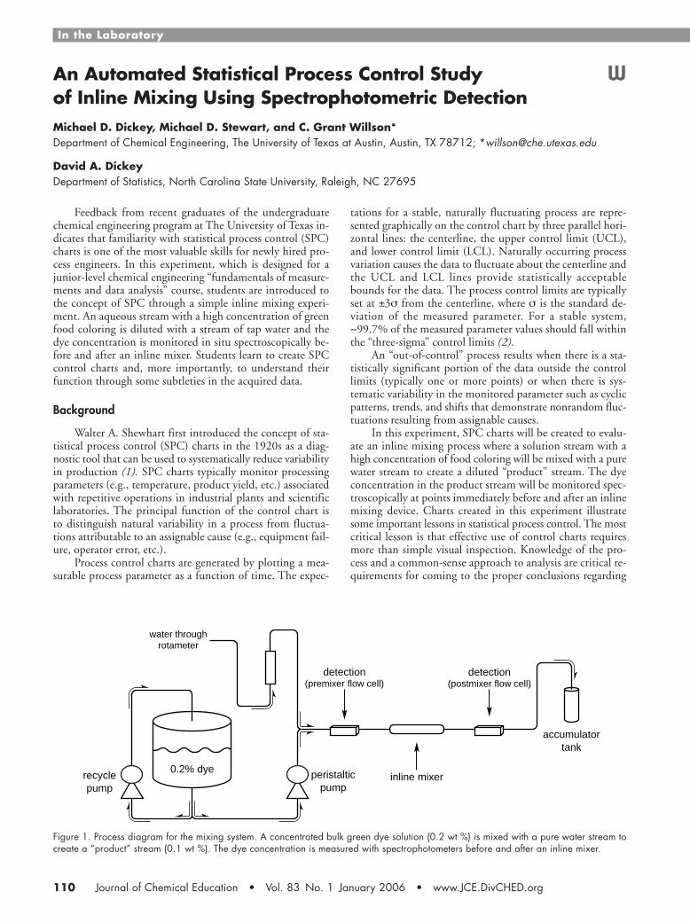
Figure 1. Process diagram for the mixing system. A concentrated bulk green dye solution (0.2 wt %) is mixed with a pure water stream tocreate a “product” stream (0.1 wt %). The dye concentration is measured with spectrophotometers before and after an inline mixer.

detection(premixer flow cell)

inline mixerperistalticpump

0.2% dye

accumulatortank

detection(postmixer flow cell)

water throughrotameter

recyclepump

In the Laboratory

www.JCE.DivCHED.org • Vol. 83 No. 1 January 2006 • Journal of Chemical Education 111

SPC charts. Specifically, efforts to reduce variability in a pro-cess, such as adding an inline mixer, typically result in nar-rower control limits. Narrow control limits are more sensitiveto minor nonrandom fluctuations and therefore are morelikely to produce out-of-control results. The key is for stu-dents to recognize this tradeoff and make the proper recom-mendations for handling sensitive control limits.

Experimental Procedure

A diagram of the experimental process is shown in Fig-ure 1, where a feed stream of green dye solution is mixedwith a pure water stream to create a “product” stream with alower dye concentration. Green food coloring (Adam’s Ex-tract) is used as the process dye and a pair of spectropho-tometers are used for detection. Full details for the equipmentand materials are given in the Supplemental Materials.W

The students should be familiar with the basic conceptof control charts from the lecture portion of the class. Thestudents are required to perform several simple tasks duringthe experiment: mix the feedstock solution, calibrate the waterflow meter prior to beginning the data acquisition, and makesimple calculations using Lambert–Beer law. The spectropho-tometer comes with user-friendly software but may require abriefing by the instructor prior to operation.

At least 500 absorbance measurements are taken of justthe feedstock stream, which is used for analysis of the vari-ability of the detectors and to determine the concentrationof the feedstock solution. Following these measurements, thepure water stream is set to the appropriate flow rate to dilutethe feedstock stream to 0.1 wt %. A minimum of 1000 ab-sorbance measurements are taken on this process stream (ata rate of about 1 per second). These experimental data arethen used to generate SPC charts. The entire experiment canbe performed in two hours.

Hazards

A safe, nontoxic food coloring should be used as the pro-cess dye. Some care should be taken to position electrical equip-ment (pumps, computer, spectrophotometer lamp) in dry areasaway from any potential dripping or leaking piping.

Results and Discussion

The primary pedagogical goal of this experiment is toteach students how to create and analyze SPC charts by evalu-ating the effects of the inline mixer on the dye mixing pro-cess. These charts can be quickly produced using a statisticalsoftware package (e.g., JMP, SAS Institute) or using a spread-sheet program such as Microsoft Excel. Students are requiredto provide sample hand calculations in the lab report to avoidan overreliance on “black box” computer programs.

Some typical raw data from this experiment are shownin Figure 2, where absorbance has been converted to dye con-centration via Beer’s Law. It is readily apparent that concen-tration fluctuations are much greater in the premixer readingsthan in the postmixer readings, which implies that the inlinemixer is effectively reducing concentration variations.

The students convert the raw data into control chart for-mat, breaking down the data into subgroups of size n = 5.

Subgroups intervals are chosen such that the variation withineach subgroup is attributable to only natural process varia-tion. This is often accomplished by picking a time intervalthat is short relative to any possible systematic process varia-tion. Figures 3 and 4 present the pre- and postmixer data inthe two control chart formats, X

– chart and R (range) chart.

X– charts plot the average value of each subgroup, while Rcharts plot the range of each subgroup, a measure of vari-ability (see the Supplemental MaterialW for details on the for-mation of control charts). As expected, the measuredvariability is lower after the stream passes through the inlinemixer. Based on the R– values found on the R charts in Fig-ures 3B and 4B, the mixer reduces concentration variationby a factor of 13. Students are asked to consider why de-creased variance is important to the process by becoming fa-miliar with the process capability index (Cp). Cp is the ratioof product tolerance limits to the process control limits, whichprovides a useful heuristic for evaluating the ability of a pro-cess to meet given product specifications. The students willfind that the premixer and postmixer capability values differsignificantly. The premixer process has a Cp value of about0.2 versus a value of about 1.6 for the postmixer (using speci-fication limits of 0.100 ± 0.002 wt %). Generally, a Cp of atleast 1.3 is desired to ensure that the product meets specifi-cation. Thus, the calculation of Cp clearly demonstrates theimportance of the mixer in assuring the product is actuallymeeting specifications.

Intuition suggests to most students that having an inlinemixer will provide an improvement in variance over not hav-ing a mixer in the process stream. This intuition is validatedby the dramatic reduction in variability achieved by the inlinemixer, as seen in Figure 2 and by the corresponding increasein Cp obtained through use of the mixer. Despite these im-provements, a non-discerning examination of the SPC chartscould lead to the incorrect conclusion that the inline mixeris detrimental to the process. The postmixer X– chart (Figure4A) shows that the process is out-of-control because thereare numerous points outside the control limits, which is incontrast to the premixer data. Based on this purely statisticalanalysis, the inline mixer has seemingly made things “worse”not “better”. This apparent contradiction between simplistic

Figure 2. Typical dye concentration data for the premixer andpostmixer measured spectroscopically. The data demonstrate thedramatic decrease in variability achieved by the inline mixer and,consequently, the improved process capability.

In the Laboratory

112 Journal of Chemical Education • Vol. 83 No. 1 January 2006 • www.JCE.DivCHED.org

chart reading and common sense expectations provides a pow-erful learning tool. The ability of the inline mixer to homog-enize the solution reduces the postmixer variability, whichin turn results in narrower control limits for the postmixer.Consequently, the postmixer control charts are more sensi-tive to small processing fluctuations that are otherwisedrowned out by the large variability in the premixer data.Narrow control limits rapidly alert the observer to small non-random fluctuations, but are also more likely to detect non-significant process variations. Therefore, it is critical thatthe student understands both the source and the impact ofany assignable variations to determine whether the sourceshould be addressed or neglected.

The primary reason the postmixer data in Figure 4A areout-of-control is due to the presence of systematic trends inthe data. The trends in the data are known as “autocorrela-tion”, where successive measurements are not independent.Although rigorous methods exist to quantify autocorrelation,a simple test is suggested in the lab handout to prove thedata are nonrandom. The method involves randomizing theorder of the data as a function of time and recalculating the

control charts. If the data are truly random, then the orderof the data should have no affect on the control charts. How-ever, after randomizing the data, the average range (R– ) typi-cally increases by a factor of 5–10 for the postmixer data.This simple analysis proves the fluctuations are nonrandomand implies that the data are correlated.

In the final step of the analysis, students must identifythe source of the nonrandom trends. The most likely culpritis nonconstant water flow rates owing to changing water pres-sure in the building manifold. Careful observation of the rota-meter on the water line would reveal slight fluctuations duringthe experiment. The sensitive control limits of the postmixercharts are capable of detecting these small process fluctua-tions. The premixer charts are incapable of detecting thesefluctuations due to the magnitude of the variations causedby poor mixing.

Based on their analysis, students must make recommen-dations for a future course of action, such as eliminating theassignable causes of variation or reevaluating the control limitsin light of the processing requirements. Typically when a pro-cess is out-of-control, the source of nonrandom fluctuations

Figure 3. Example SPC charts from the premixer detector duringmixing trial: (A) X

– chart and (B) R chart.

A

B

UCLAVGLCL

Subgroup Number

Sub

grou

p C

once

ntra

tion

(wt %

)

0.096

0.098

0.100

0.102

0.104

0.106

0 50 100 150 200 250 300

= 0.1006= 0.1053

= 0.0960

Subgroup Number

0.0000 50 100 150 200 250 300

0.004

0.008

0.012

0.016

UCL

AVG

LCL

= 0.0171

= 0.0081

= 0.0000

Sub

grou

p R

ange

(wt %

)

Figure 4. Example SPC charts from the postmixer detector duringmixing trial: (A) X

– chart and (B) R chart.

A

B

Subgroup Number

Sub

grou

p C

once

ntra

tion

(wt %

)

0.0995

0.1000

0.1010

0.1005

0.1015

0 50 100 150 200 250 300

UCL

AVG

LCL

= 0.1006

= 0.1010

= 0.1003

UCL

AVG = 0.0006

LCL

= 0.0013

= 0.0000

Subgroup Number

Sub

grou

p R

ange

(wt %

)

0.0000

0.0002

0.0004

0.0006

0.0008

0.0010

0.0012

0.0014

0.0016

0 50 100 150 200 250 300

In the Laboratory

www.JCE.DivCHED.org • Vol. 83 No. 1 January 2006 • Journal of Chemical Education 113

must be removed. However, since all of the data fall withinthe processing requirements, reevaluation of the control limitswould be the least expensive corrective action.

Conclusions

An experiment designed to teach students the power ofSPC charts was presented. The students learn how to createand analyze control charts in an effort to evaluate the ben-efits of a mixer. The experimental configuration is useful forstatistical analysis since the spectrophotometer detectors canrapidly acquire many data points. An important componentof the pedagogical power of this experiment lies in the seem-ingly contradictory nature of the data obtained, which forcesthe students to develop a deeper understanding of controlcharts. The experimental results show that the mixer clearlyreduces measured variability in dye concentration. However,the reduction in variability narrows the control limits, mak-ing the postmixer control charts hypersensitive to minor pro-cess fluctuations. The consequence of this effect is that thepostmixer data are technically out-of-control whereas thepremixer data are “in-control” despite having significantlygreater process variance. The source of the out-of-control datacan be logically narrowed down to a single assignable cause:variation in water flow rate. Students are forced to justify acourse of action based on the analysis of the control charts.Options include modifying the control limits or eliminatingsources of nonnatural variability.

Acknowledgments

We are grateful to Pavlos Tsiartas for assistance with theoptics for the spectrophotometer.

WSupplemental Material

An expanded version of the text, a detailed experimen-tal procedure for the students, notes for the instructor, and aprelab quiz are available in this issue of JCE Online. The tech-niques to create SPC charts are well established and can befound in most general statistics books (3–5).

Literature Cited

1. Shewhart, W. A. Economic Control of Quality of ManufacturedProduct; D. Van Nostrand Company Inc.: New York, 1931.

2. Wheeler, D. J.; Chambers, D. S. Understanding Statistical Pro-cess Control; Statistical Process Controls: Knoxville, TN, 1986;pp 72–83.

3. John, P. W. M. Statistical Methods in Engineering and QualityAssurance; Wiley: New York, 1990.

4. Walpole, R. E. Probability & Statistics for Engineers & Scien-tists, 7th ed.; Prentice Hall: Upper Saddle River, NJ, 2002;pp 625–635.

5. Miller, I.; Freund, J. E.; Johnson, R. A. Miller and Freund’sProbability and Statistics for Engineers; Prentice Hall: Engle-wood Cliffs, NJ, 1994; pp 516–523.