An attempt to model ion conductance when a SICM approaches a

1

An attempt to model ion

conductance when a SICM approaches a flat surface

Author: William Fletcher1 Supervisors: Dr. G Moss2

Dr . A Shevchuk3 1CoMPLEX (Centre for Mathematics and Physics in the Life Sciences and Experimental Biology), UCL (University College London), NW1 2HE, UK 2Dept. of Pharmacology, UCL (University College London), WC1E 7JE, UK 3Division of Medicine, Imperial College London, Hammersmith Hospital Campus, Du Cane Road, London, W12 0NN.

Abstract Scanning Ion Conductance Microscopy, it’s development, design and use are introduced. The theory behind modelling ion current flow into the SICM probe tip and the problems involved with analytically modelling the current flow are then briefly discussed. A numerical simulation using the Finite Difference Method is then used to model the current flow as the microscope probe tip approaches a flat non conducting surface.

2

Introduction This section introduces various types of scanning probe microscope, the Scanning Ion Conductance Microscope (SICM) in particular, and discusses their relative merits in application to biological imaging. The SICM, its construction, design and use is then outlined in more detail. Scanning Probe Microscopy A SICM (Scanning Ion Conductance Microscope) is a member of a family of microscopes, known collectively as SPMs (Scanning Probe Microscopes). SICMs will be discussed in greater detail in the next section, but first SPMs. and microscopy in general, will be introduced. When analysing a sample, optical microscopes have the great advantage that they are non-invasive. However, they are limited in resolution by the wavelength of visible light, which is made up of photons. One alternative is electron beam microscopes, which employ electrons in place of photons, and use magnets rather than lenses to focus the image. Electrons have a wavelength that is thousands of times smaller than that of photons so image resolution is greatly increased. However, samples being analysed have to be electrically conducting and electrons cannot be routed into living organisms, and biological samples, without causing undesired side effects. SPMs offer a variety of alternatives to these two approaches. SPMs allow measurement and imaging of objects in comparable detail to electron microscopy when compared to conventional optical microscopy. They can achieve molecular, and even atomic, resolution by means of a “probe” which is used to “scan” over the sample that one wants to investigate. The SPM family has many members that are well known by their own acronyms: STM, AFM and NSOM, to name but a few. Each has their own distinct detecting capabilities, and advantages and disadvantages related to their use, that largely depends on the type of sample that one wants to image. A few examples of SPMs are given below: STM: Binnig et al. [1] first demonstrated the use of STMs (Scanning Tunneling Microscopes) in 1982. An STM works by measuring a weak electrical current flowing between a sample and a very sharp metal wire tip that is used as a probe. The tip is held a very small distance from the sample (on the order of nanometres) and classically there should be no net current flow between the two. However, the STM exploits an effect known as “tunnelling”. Tunnelling is a quantum mechanical property where electrons move through barriers that they shouldn’t be allowed to move through according to classical theory. Using STMs to image biological samples poses two main problems. Firstly biological samples have low conductivities and secondly there is the issue of how to reliably place

3

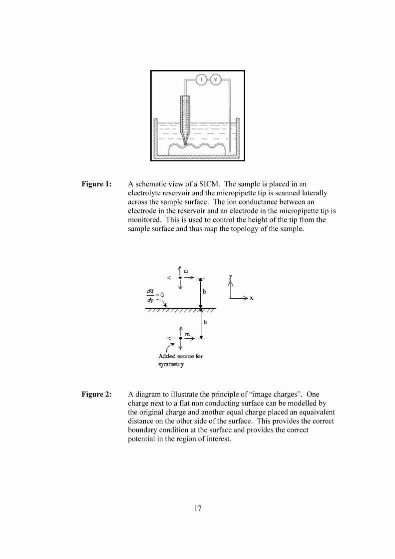
the sample on a flat conducting surface. Attempts have been made to solve these problems by Garcia et al. [2] when they coated biological samples with a thin film of platinum-carbon. Although this method may prove useful in some scenarios, it is far from the non-invasive method that biologists seek for most applications. AFM: Also first demonstrated by Binnig et al. [3]. An AFM (Atomic Force Microscope) employs a cantilever probe with a very sharp tip to measure samples. The microscope measures the interaction force, between its probe tip and the sample, by dragging the tip across the sample in much the same way as a stylus on a record player is dragged across the surface of a record. The information from the tip can then be used to map the sample surface topology. One advantage of AFMs is that they can be used in a variety of modes to measure other sample properties such as the magnetic field of the surface or the surface thermal conductivity properties. A disadvantage is that the sharp probe tip can damage soft samples, especially those of a biological nature, as shown by Henderson et al. [4] and You et al. [5]. Lewis et al. first described the use of a NSOM (Near-Field Scanning Optical Microscope) in 1984 [6]. NSOMs scan a small light source (normally a laser) over a sample and the detection of the energy from the reflected light is used to construct the image. Using this approach, image resolutions can be achieved that are an order of magnitude greater than conventional Far-Field Optical Microscopes. The application of NSOMs to the biological sciences is fraught with problems. For example, they are not well designed to deal with “wet samples” due to the varying optical properties (of the medium between microscope and sample) that may be encountered. The most significant problem is the control of the distance between the near field aperture and the sample, as discussed by Edidin [7], who believes that the application of NSOM to biology is only at a comparable stage to where electron microscopy was 40 or 50 years ago. Scanning Ion Conductance Microscopy The principle of Scanning Ion Conductance Microsopy was first developed by Hansma et al. [8] in 1989. Unlike other SPMs the SICM was designed specifically for biology and electrophysiology [8] in that it can image soft-non conductors, such as cell membranes, that are covered in electrolytes (although it wasn’t used for that purpose by Hansma). The original schematic view of the SICM provided by Hansma et al. in [8] is shown in Figure 1. In a SICM, a glass micropipette filled with electrolyte is used as a probe, and the sample to be analysed is placed in a reservoir of electrolyte. The tip is then lowered towards an insulating sample whilst the conductance, between an electrode inside the micropipette and another electrode in the electrolyte reservoir, is monitored. The probe tip’s position in relation to the sample surface strongly affects this measured ion conductance. As the micropipette tip is brought closer to the surface the space through which ions can flow is decreased, and so the ion current also decreases.

4

Once a reference level of ion conductance has been chosen, the micropipette is scanned laterally across the sample whilst a feedback loop alters the vertical position of the tip so that the level of conductance remains at this reference level. This has the effect of maintaining the probe tip to sample separation at a constant distance, and enables the topology of the sample surface to be mapped at very high resolutions without the tip of the micropipette ever making direct contact with the sample. A brief look at the development and use of SICM Variations on the general principle of SICM have been proposed over the years. Prater et al. [9] demonstrated a SICM with a more robust fabricated silicon tip in 1991, and Proksch et al. [10] developed a “tapping mode” SICM that used a bent micropipette tip as both a cantilever and a current sensitive probe. However, all these studies [8,9,10] have one thing in common - they involved imaging flat polymeric films and not biological samples or living cells. Using a SICM for this purpose, with the now familiar “feedback control” was first described by Korchev et al. [11,12] in 1997. In these papers the ion current flow characteristics of a SICM in relation to tip/sample separation distance is discussed in detail, and these works will be returned to in greater detail in the later sections. Since 1997, SICM has shown advantages over other types of microscopy in a variety of fields, and found many diverse applications in the biological sciences. In 2000, Korchev et al [13] found a novel use of the SICM to measure cell volumes whilst retaining cell functionality. Their method works over a wide range of cell volumes and the cellular processes, surface characteristics and volumes can all be measured simultaneously. Also in 2000, another group, also lead by Korchev, used SICM for the first time to map single active ion channels whilst simultaneously imaging intact cellular membranes [14]. This ability to measure more than one property at once is an advantage of SICM that crops up repeatedly. In 2002, Gorelik et al. incorporated SICM in a method for simultaneous recording of high resolution topography and cell surface fluorescence in a single scan [15]. In the same year, Gorelik led another group that exploited the fact that SICM and patch clamp recording both use a micropipette as a probe to incorporate the two processes into one. Using the same tip facilitated single ion channel recording from small cells and submicron cellular structures that are inaccessible by conventional methods [16]. Despite the widespread application of SICM to a variety of problems there is still a relative lack of understanding in precisely how the ion conductance varies as the probe tip scans over small topological features of a size comparable to the pipette tip radius. Although this does not represent a problem in a large number of applications it is an obvious gap in the theory behind SICM, as ion conductance is crucial in determining the tip height above the sample. There is not only an absence of analytical formulas to describe how ion conductance varies but an absence of numerical approximations for all but the simplest of scenarios. The reasons behind this are discussed in the next section and possible approaches to solving the problem are investigated.

5

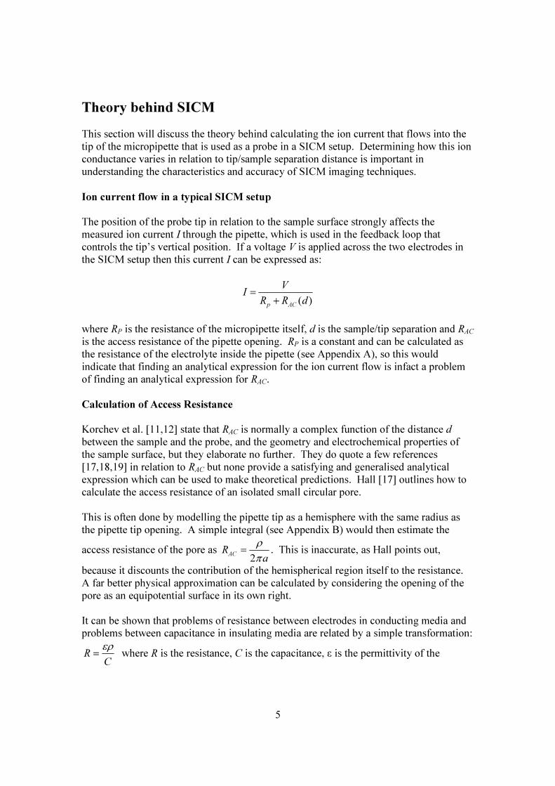
Theory behind SICM This section will discuss the theory behind calculating the ion current that flows into the tip of the micropipette that is used as a probe in a SICM setup. Determining how this ion conductance varies in relation to tip/sample separation distance is important in understanding the characteristics and accuracy of SICM imaging techniques. Ion current flow in a typical SICM setup The position of the probe tip in relation to the sample surface strongly affects the measured ion current I through the pipette, which is used in the feedback loop that controls the tip’s vertical position. If a voltage V is applied across the two electrodes in the SICM setup then this current I can be expressed as: ( )p AC

VIR R d

=+

where RP is the resistance of the micropipette itself, d is the sample/tip separation and RAC is the access resistance of the pipette opening. RP is a constant and can be calculated as the resistance of the electrolyte inside the pipette (see Appendix A), so this would indicate that finding an analytical expression for the ion current flow is infact a problem of finding an analytical expression for RAC. Calculation of Access Resistance Korchev et al. [11,12] state that RAC is normally a complex function of the distance d between the sample and the probe, and the geometry and electrochemical properties of the sample surface, but they elaborate no further. They do quote a few references [17,18,19] in relation to RAC but none provide a satisfying and generalised analytical expression which can be used to make theoretical predictions. Hall [17] outlines how to calculate the access resistance of an isolated small circular pore. This is often done by modelling the pipette tip as a hemisphere with the same radius as the pipette tip opening. A simple integral (see Appendix B) would then estimate the access resistance of the pore as

2ACRa

ρπ

= . This is inaccurate, as Hall points out, because it discounts the contribution of the hemispherical region itself to the resistance. A far better physical approximation can be calculated by considering the opening of the pore as an equipotential surface in its own right. It can be shown that problems of resistance between electrodes in conducting media and problems between capacitance in insulating media are related by a simple transformation: R

Cερ

= where R is the resistance, C is the capacitance, ε is the permittivity of the

6

medium where the capacitance is measured, and ρ is the resistivity of the medium where the resistance is measured. So if the circular mouth of the pore is considered an equipotential surface then the problem of calculating access resistance reduces to that of calculating the capacitance of a conducting disk to a half spherical electrode at infinity. Using the well known result [20] that the capacitance of a charged conducting disk of radius a is: 8C aε= a new estimate of the access resistance is calculated as

4ACRaρ

= . This value is a factor of / 2π larger than the previous estimate, and represents the access resistance of an isolated micropipette tip of radius a, in an electrolyte solution with specific resistivity ρ. Clearly any analytical expression for access resistance would then have to satisfy ( ) 4ACR d for d aa

ρ→ >> . Explicit expressions for access resistance

and current flow, that satisfy this condition have been found for other forms of microscopy [21]. No such expressions have yet been calculated for SICM. Attempt to find analytical expression for Access Resistance and Ion Conductance It is well known that all electrostatical problems can be reduced to solving Laplace’s equation, on a compact region, provided all boundary conditions are known. Laplace’s equation in familiar Cartesian coordinates is given by:

2 2 2

2 2 2 0x y zφ φ φ∂ ∂ ∂+ + =

∂ ∂ ∂

where φ is the electrostatic potential. If the charged disk (i.e. pipette opening) is in the x,y plane, i.e. the axis of the disk is parallel to the z axis then the current density i at the disk surface can be calculated as

0

1z

izφ

ρ=

∂= −∂

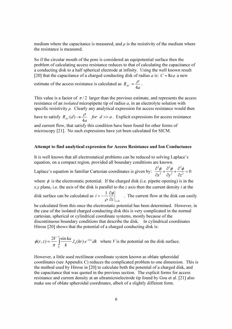
. The current flow at the disk can easily be calculated from this once the electrostatic potential has been determined. However, in the case of the isolated charged conducting disk this is very complicated in the normal cartesian, spherical or cylindrical coordinate systems, mostly because of the discontinuous boundary conditions that describe the disk. In cylindrical coordinates Hirose [20] shows that the potential of a charged conducting disk is:

| |0

0

2 sin( , ) ( ) k zV kar z J kr e dkk

φ π∞

−= ∫ where V is the potential on the disk surface.

However, a little used rectilinear coordinate system known as oblate spheroidal coordinates (see Appendix C) reduces the complicated problem to one dimension. This is the method used by Hirose in [20] to calculate both the potential of a charged disk, and the capacitance that was quoted in the previous section. The explicit forms for access resistance and current density at an ultramicroelectrode tip found by Gou et al. [21] also make use of oblate spheroidal coordinates, albeit of a slightly different form.

7

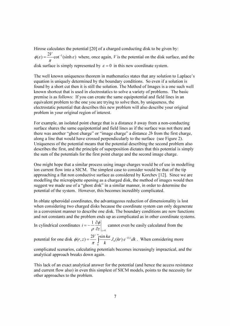
Hirose calculates the potential [20] of a charged conducting disk to be given by:

12( ) cot (sinh )Vφ ε επ−

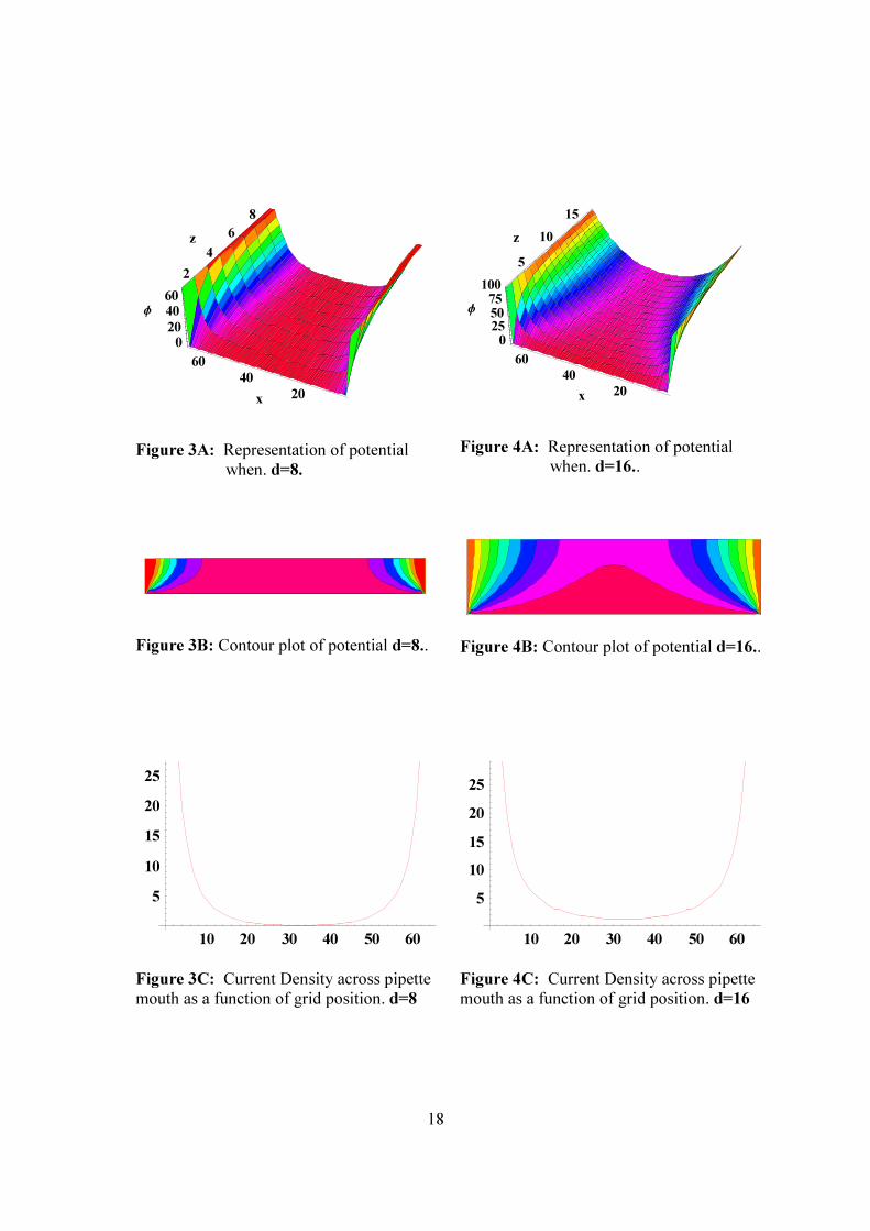
= where, once again, V is the potential on the disk surface, and the disk surface is simply represented by 0ε = in this new coordinate system. The well known uniqueness theorem in mathematics states that any solution to Laplace’s equation is uniquely determined by the boundary conditions. So even if a solution is found by a short cut then it is still the solution. The Method of Images is a one such well known shortcut that is used in electrostatics to solve a variety of problems. The basic premise is as follows: If you can create the same equipotential and field lines in an equivalent problem to the one you are trying to solve then, by uniqueness, the electrostatic potential that describes this new problem will also describe your original problem in your original region of interest. For example, an isolated point charge that is a distance b away from a non-conducting surface shares the same equipotential and field lines as if the surface was not there and there was another “ghost charge” or “image charge” a distance 2b from the first charge, along a line that would have crossed perpendicularly to the surface (see Figure 2). Uniqueness of the potential means that the potential describing the second problem also describes the first, and the principle of superposition dictates that this potential is simply the sum of the potentials for the first point charge and the second image charge. One might hope that a similar process using image charges would be of use in modelling ion current flow into a SICM. The simplest case to consider would be that of the tip approaching a flat non conductive surface as considered by Korchev [12]. Since we are modelling the micropipette opening as a charged disk, the method of images would then suggest we made use of a “ghost disk” in a similar manner, in order to determine the potential of the system. However, this becomes incredibly complicated. In oblate spheroidal coordinates, the advantageous reduction of dimensionality is lost when considering two charged disks because the coordinate system can only degenerate in a convenient manner to describe one disk. The boundary conditions are now functions and not constants and the problem ends up as complicated as in other coordinate systems. In cylindrical coordinates

0

1z

izφ

ρ=

∂= −∂

cannot even be easily calculated from the

potential for one disk | |0

0

2 sin( , ) ( ) k zV kar z J kr e dkk

φ π∞

−= ∫ . When considering more

complicated scenarios, calculating potentials becomes increasingly impractical, and the analytical approach breaks down again. This lack of an exact analytical answer for the potential (and hence the access resistance and current flow also) in even this simplest of SICM models, points to the necessity for other approaches to the problem.

8

Method - numerical approximation of ion current flow This section discusses a numerical approach to modelling ion current flow into a SICM micropipette tip. An outline is given of the assumptions made then the simulation process is described in more detail. Aims of the simulation Korchev et al [11,12] found a characteristic (experimentally verified) curve that relates ion current flow and tip/sample separation distance when modelling a SICM approaching a flat non conductive surface. The aim of this paper is to create a simple simulation that accurately models this relationship and recreates this characteristic relation. It was the intention to try and create a simulation that could be adapted to investigating current flow when a SICM approaches surfaces with other simple, non-flat topologies. Finite Difference Method (FDM) FDM (see Appendix D) is a well known method for finding solutions to partial differential equations (PDEs). Using Mathematica, FDM was used to solve Laplace’s equation according to certain boundary conditions that were chosen according to the following assumptions. Basic Assumptions of the model

• The problem of modelling current flow into the probe tip as it approaches a flat surface will exhibit radial symmetry so the problem can be considered as two dimensional.

• We will assume that the pipette opening can be modelled as a disk of radius a that

lies in the plane y=1. For the purposes of the 2D simulation, the disk will be modelled by a radial slice, so the disk will take the form of a line of grid points along the bottom of the simulation region.

• The flat surface shall be taken as being at y=d , and shall form a line of grid

points along the top boundary of the simulation region. The number d therefore represents the distance between sample and probe tip.

• If the coordinate x represents radial distance from the disk axis, then the

simulation region is a rectangle 2a grid points wide and d points high. The top boundary represents a portion of the flat surface. The bottom boundary is a radial cross section of the pipette opening which current flows through. The left and right boundaries represent the interaction between the simulation region and the rest of the electrolyte. It is through these left and right boundaries that any ion current must arrive in the simulation.

9

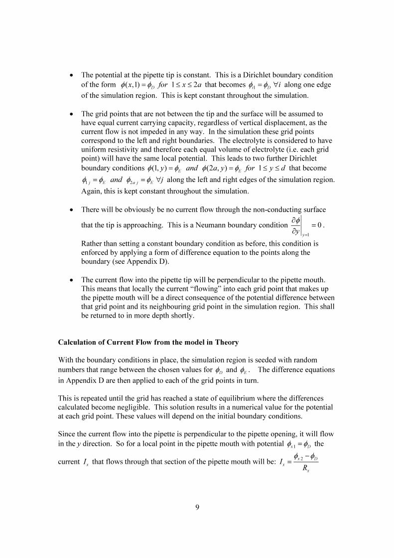
• The potential at the pipette tip is constant. This is a Dirichlet boundary condition of the form ( ,1) 1 2Dx for x aφ φ= ≤ ≤ that becomes 1i D iφ φ= ∀ along one edge of the simulation region. This is kept constant throughout the simulation.

• The grid points that are not between the tip and the surface will be assumed to

have equal current carrying capacity, regardless of vertical displacement, as the current flow is not impeded in any way. In the simulation these grid points correspond to the left and right boundaries. The electrolyte is considered to have uniform resistivity and therefore each equal volume of electrolyte (i.e. each grid point) will have the same local potential. This leads to two further Dirichlet boundary conditions (1, ) (2 , ) 1E Ey and a y for y dφ φ φ φ= = ≤ ≤ that become 1 2j E a j Eand jφ φ φ φ= = ∀ along the left and right edges of the simulation region.

Again, this is kept constant throughout the simulation.

• There will be obviously be no current flow through the non-conducting surface that the tip is approaching. This is a Neumann boundary condition

1

0yy

φ=

∂ =∂

.

Rather than setting a constant boundary condition as before, this condition is enforced by applying a form of difference equation to the points along the boundary (see Appendix D).

• The current flow into the pipette tip will be perpendicular to the pipette mouth.

This means that locally the current “flowing” into each grid point that makes up the pipette mouth will be a direct consequence of the potential difference between that grid point and its neighbouring grid point in the simulation region. This shall be returned to in more depth shortly.

Calculation of Current Flow from the model in Theory With the boundary conditions in place, the simulation region is seeded with random numbers that range between the chosen values for Dφ and Eφ . The difference equations in Appendix D are then applied to each of the grid points in turn. This is repeated until the grid has reached a state of equilibrium where the differences calculated become negligible. This solution results in a numerical value for the potential at each grid point. These values will depend on the initial boundary conditions. Since the current flow into the pipette is perpendicular to the pipette opening, it will flow in the y direction. So for a local point in the pipette mouth with potential 1x Dφ φ= the current xI that flows through that section of the pipette mouth will be: 2x D

xx

IR

φ φ−=

10

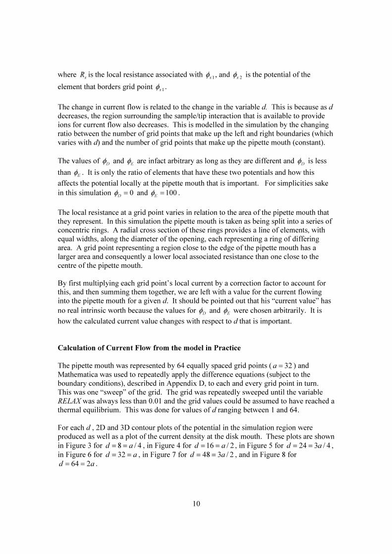
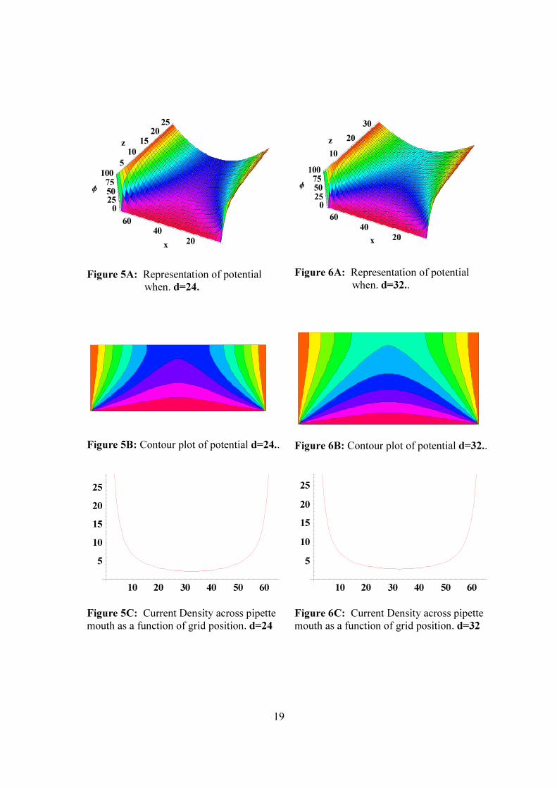
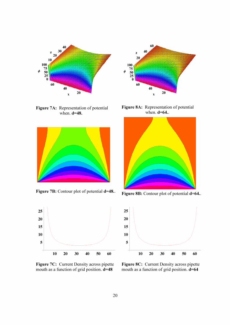
where xR is the local resistance associated with 1xφ , and 2xφ is the potential of the element that borders grid point 1xφ . The change in current flow is related to the change in the variable d. This is because as d decreases, the region surrounding the sample/tip interaction that is available to provide ions for current flow also decreases. This is modelled in the simulation by the changing ratio between the number of grid points that make up the left and right boundaries (which varies with d) and the number of grid points that make up the pipette mouth (constant). The values of Dφ and Eφ are infact arbitrary as long as they are different and Dφ is less than Eφ . It is only the ratio of elements that have these two potentials and how this affects the potential locally at the pipette mouth that is important. For simplicities sake in this simulation 0Dφ = and 100Eφ = . The local resistance at a grid point varies in relation to the area of the pipette mouth that they represent. In this simulation the pipette mouth is taken as being split into a series of concentric rings. A radial cross section of these rings provides a line of elements, with equal widths, along the diameter of the opening, each representing a ring of differing area. A grid point representing a region close to the edge of the pipette mouth has a larger area and consequently a lower local associated resistance than one close to the centre of the pipette mouth. By first multiplying each grid point’s local current by a correction factor to account for this, and then summing them together, we are left with a value for the current flowing into the pipette mouth for a given d. It should be pointed out that his “current value” has no real intrinsic worth because the values for Dφ and Eφ were chosen arbitrarily. It is how the calculated current value changes with respect to d that is important. Calculation of Current Flow from the model in Practice The pipette mouth was represented by 64 equally spaced grid points ( 32a = ) and Mathematica was used to repeatedly apply the difference equations (subject to the boundary conditions), described in Appendix D, to each and every grid point in turn. This was one “sweep” of the grid. The grid was repeatedly sweeped until the variable RELAX was always less than 0.01 and the grid values could be assumed to have reached a thermal equilibrium. This was done for values of d ranging between 1 and 64. For each d , 2D and 3D contour plots of the potential in the simulation region were produced as well as a plot of the current density at the disk mouth. These plots are shown in Figure 3 for 8 / 4d a= = , in Figure 4 for 16 / 2d a= = , in Figure 5 for 24 3 / 4d a= = , in Figure 6 for 32d a= = , in Figure 7 for 48 3 / 2d a= = , and in Figure 8 for

64 2d a= = .

11

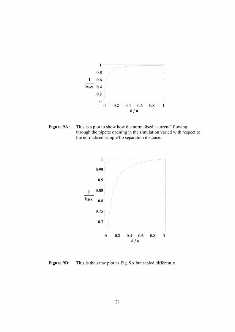
The “current value” was also calculated and stored for each d and, once normalised with respect to the calculated current value when d =a, was plotted to show the relationship between ion current flow and sample/tip separation in the model. This can be seen in Figure 9. After this a brief attempt to model the SICM tip approaching other non-flat surfaces was attempted. The simplest surface to consider is a step like surface. The simulation process is exactly the same except no analysis is performed on the grid points in the portion of the region corresponding to the step. The Neumann boundary condition along the top of the simulation region must be changed into three separate boundary conditions, one for each surface of the step. This corresponds to three sets of difference equation that are each applied to one surface of the step boundary in the simulation. Figures 10 to 15 show the arrangement and dimensions of the steps investigated. They are contour plots of the potential for various tip/sample separation distances d. It should be noted that d represents the distance to the top of the step in the sample surface. The current flow was modelled again through a similar process. The pipette opening was modelled as being 32 grid points wide (a=16) this time and the steps of height a/4 and a/2 were investigated in positions ¼, ½ and ¾ of the way across the pipette mouth. The current flow was calculated again, in a similar manner, for values of d ranging from 1 to 17 and the values stored for later inspection.

12

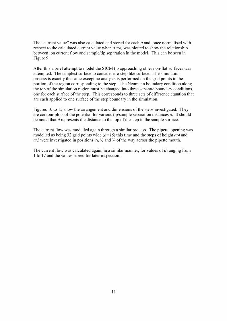
Results SICM Tip approaching a flat surface This section shall begin by discussing the graphs modelling potential and current flow that were obtained during the simulation of the tip approaching a flat surface. Figures 3A to 8A are three dimensional representations of the potential in the simulation region. The pipette mouth is represented along the bottom edge labelled x and the sample surface is the side directly opposite. Each level of potential is marked a different colour and the current flows at a tangent to the surface. The flat surface in Figure 3A shows that the region between sample and tip is all at roughly the same potential and hence there is relatively little current flow between grid points and into the pipette mouth. As d increases, the range of potentials in the simulation region (and hence the current flow in the region) increases as well. This is signified by the increase of different colours between the side representing the pipette opening and the side representing the sample surface. The current flow characteristics immediately in front of the pipette opening can be seen to change little when d becomes greater than a (Figures 6A to 8A). This can be seen more clearly in Figures 3B to 8B. They are two dimensional contour plots of the same information. The grid point potentials are colour coded and contours are drawn along lines of equal potential. The current flows along curves that cross these contours at right angles. The sample surface is represented by the top edge of the pictures and the pipette opening by the bottom edge. In the case when d=8, Figure 3B clearly shows that the simulation region shares the same potential and there is little current flow through most of the pipette opening. As d increases through Figures 3B to 8B the different contours are seen to enter the simulation region. This corresponds to a wider range of potentials in the simulation region and more current flow. For small d, as d increases, the range of colours in the local region in front of the pipette opening changes rapidly. Looking at cases of larger d, but still concentrating on this same local region, it can be seen to change little between Figures 6B and 8B. This lack of local change in front of the pipette tip suggests that the current flow through the opening levels off after d>a and reaches a maximum value. Figures 3C to 8C represent the current density along the pipette opening. In this simulation the pipette tip was modelled as a radial slice, 64 grid points long. So the point 1 and point 64 represent the very edges of the pipette opening and points 32 and 33 represent the very centre of the pipette opening. The vertical axis simply represents the amount of current flowing through a particular grid point. In all cases the current density can be seen to diverge at the exterior of the pipette opening as expected [20]. The real changes in current density happen in the centre of the pipette mouth around grid point 32.

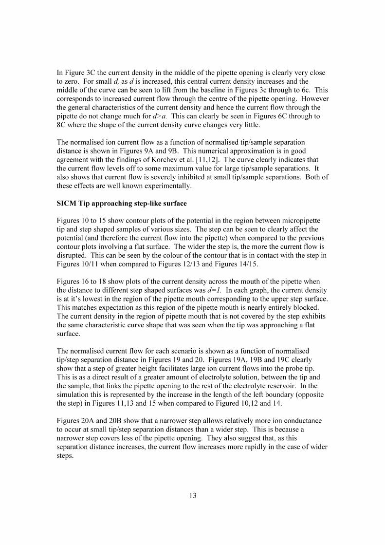
13

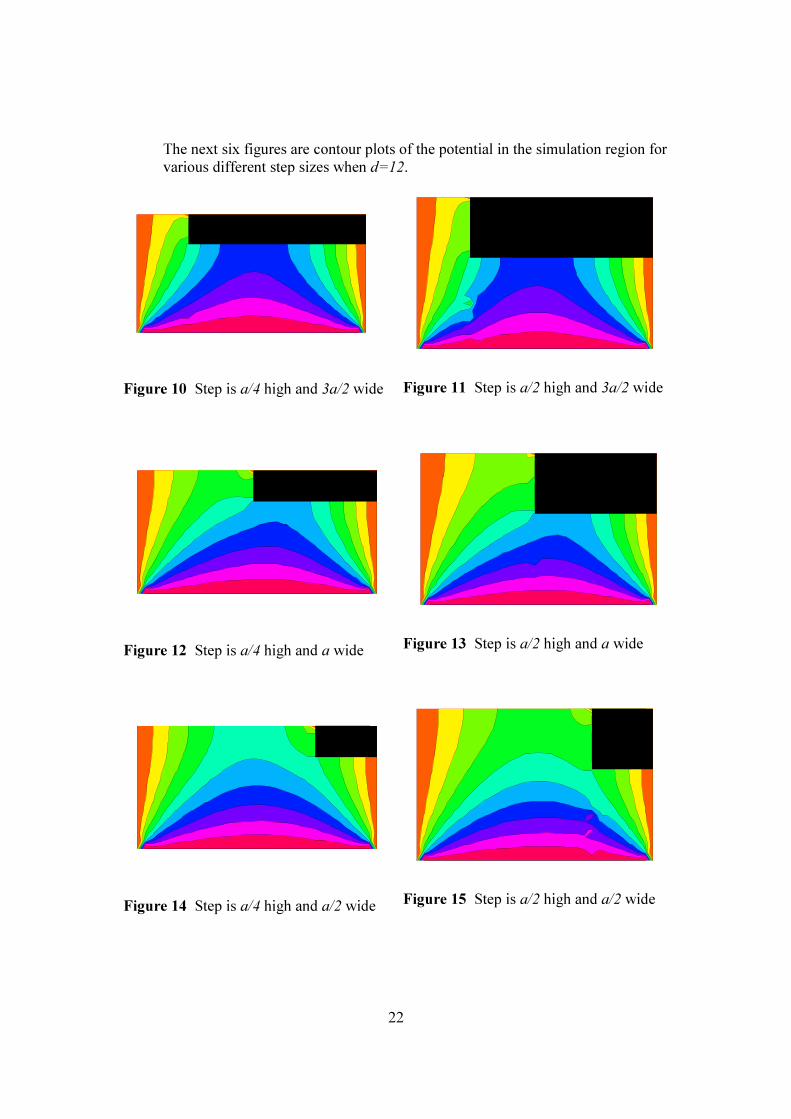
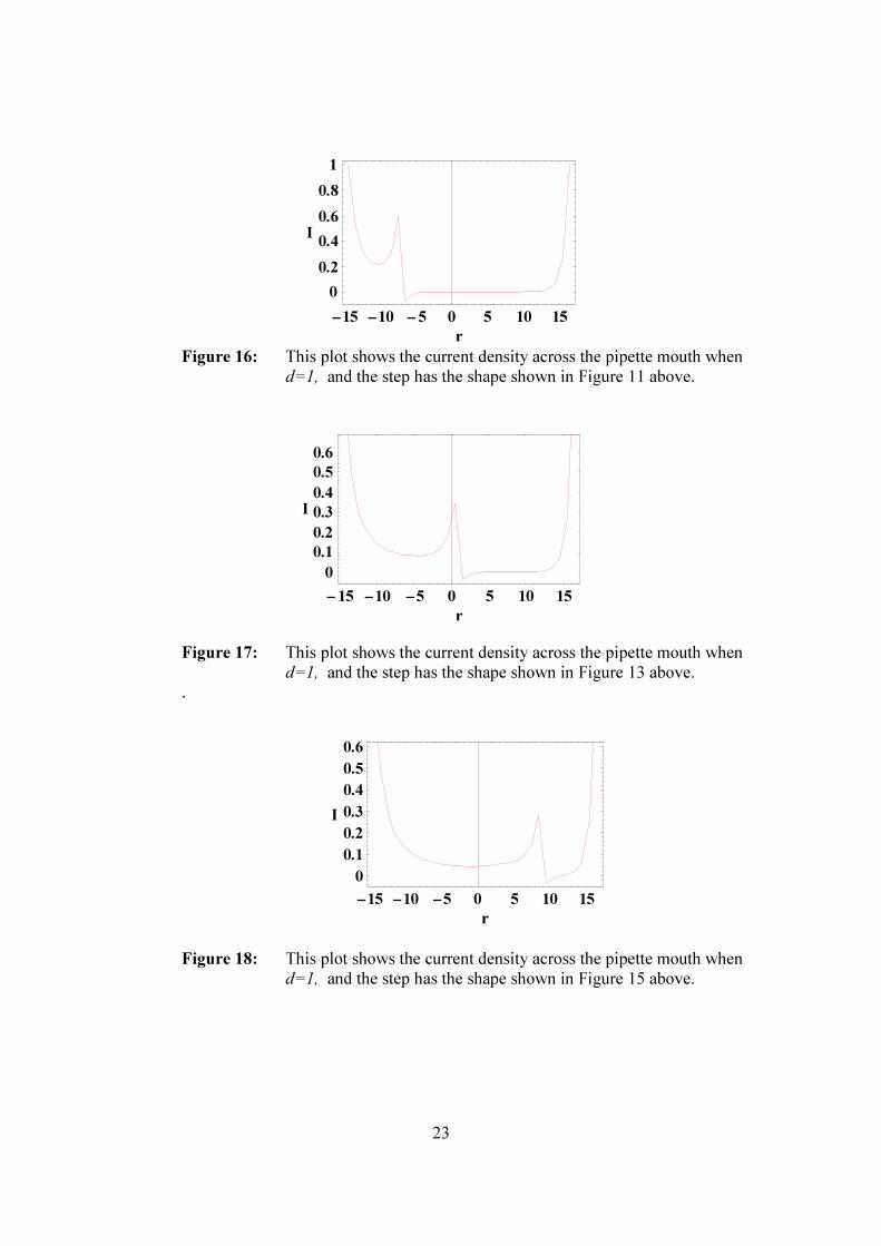
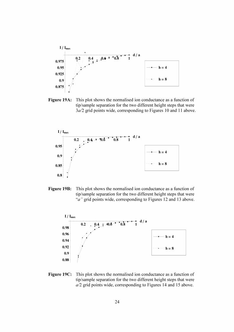
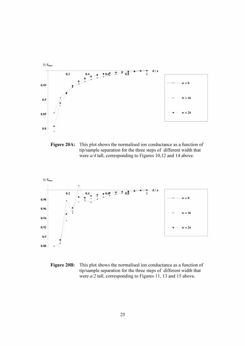
In Figure 3C the current density in the middle of the pipette opening is clearly very close to zero. For small d, as d is increased, this central current density increases and the middle of the curve can be seen to lift from the baseline in Figures 3c through to 6c. This corresponds to increased current flow through the centre of the pipette opening. However the general characteristics of the current density and hence the current flow through the pipette do not change much for d>a. This can clearly be seen in Figures 6C through to 8C where the shape of the current density curve changes very little. The normalised ion current flow as a function of normalised tip/sample separation distance is shown in Figures 9A and 9B. This numerical approximation is in good agreement with the findings of Korchev et al. [11,12]. The curve clearly indicates that the current flow levels off to some maximum value for large tip/sample separations. It also shows that current flow is severely inhibited at small tip/sample separations. Both of these effects are well known experimentally. SICM Tip approaching step-like surface Figures 10 to 15 show contour plots of the potential in the region between micropipette tip and step shaped samples of various sizes. The step can be seen to clearly affect the potential (and therefore the current flow into the pipette) when compared to the previous contour plots involving a flat surface. The wider the step is, the more the current flow is disrupted. This can be seen by the colour of the contour that is in contact with the step in Figures 10/11 when compared to Figures 12/13 and Figures 14/15. Figures 16 to 18 show plots of the current density across the mouth of the pipette when the distance to different step shaped surfaces was d=1. In each graph, the current density is at it’s lowest in the region of the pipette mouth corresponding to the upper step surface. This matches expectation as this region of the pipette mouth is nearly entirely blocked. The current density in the region of pipette mouth that is not covered by the step exhibits the same characteristic curve shape that was seen when the tip was approaching a flat surface. The normalised current flow for each scenario is shown as a function of normalised tip/step separation distance in Figures 19 and 20. Figures 19A, 19B and 19C clearly show that a step of greater height facilitates large ion current flows into the probe tip. This is as a direct result of a greater amount of electrolyte solution, between the tip and the sample, that links the pipette opening to the rest of the electrolyte reservoir. In the simulation this is represented by the increase in the length of the left boundary (opposite the step) in Figures 11,13 and 15 when compared to Figured 10,12 and 14. Figures 20A and 20B show that a narrower step allows relatively more ion conductance to occur at small tip/step separation distances than a wider step. This is because a narrower step covers less of the pipette opening. They also suggest that, as this separation distance increases, the current flow increases more rapidly in the case of wider steps.

14

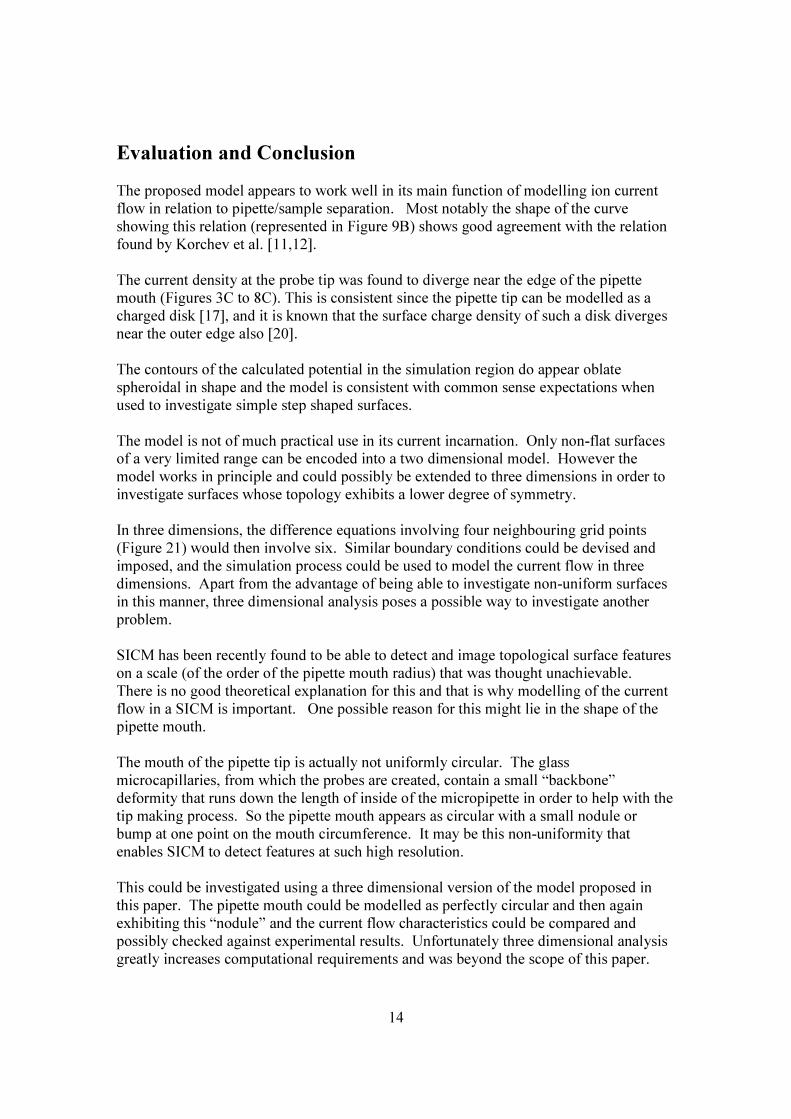
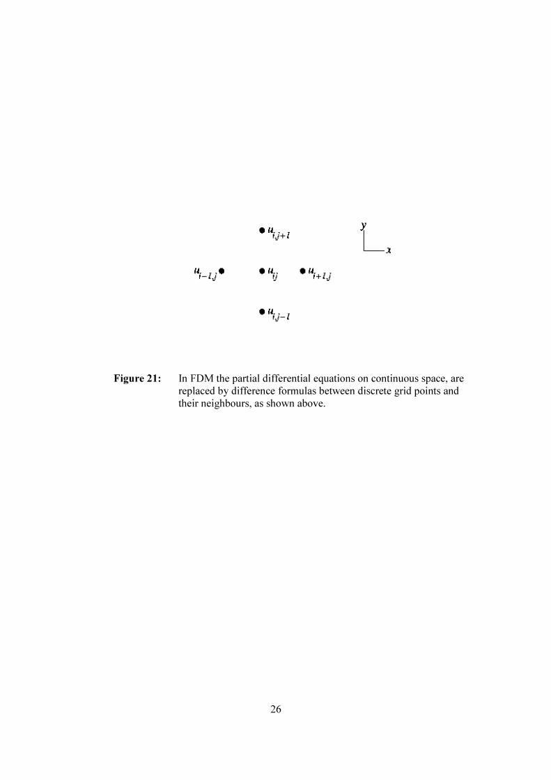
Evaluation and Conclusion The proposed model appears to work well in its main function of modelling ion current flow in relation to pipette/sample separation. Most notably the shape of the curve showing this relation (represented in Figure 9B) shows good agreement with the relation found by Korchev et al. [11,12]. The current density at the probe tip was found to diverge near the edge of the pipette mouth (Figures 3C to 8C). This is consistent since the pipette tip can be modelled as a charged disk [17], and it is known that the surface charge density of such a disk diverges near the outer edge also [20]. The contours of the calculated potential in the simulation region do appear oblate spheroidal in shape and the model is consistent with common sense expectations when used to investigate simple step shaped surfaces. The model is not of much practical use in its current incarnation. Only non-flat surfaces of a very limited range can be encoded into a two dimensional model. However the model works in principle and could possibly be extended to three dimensions in order to investigate surfaces whose topology exhibits a lower degree of symmetry. In three dimensions, the difference equations involving four neighbouring grid points (Figure 21) would then involve six. Similar boundary conditions could be devised and imposed, and the simulation process could be used to model the current flow in three dimensions. Apart from the advantage of being able to investigate non-uniform surfaces in this manner, three dimensional analysis poses a possible way to investigate another problem. SICM has been recently found to be able to detect and image topological surface features on a scale (of the order of the pipette mouth radius) that was thought unachievable. There is no good theoretical explanation for this and that is why modelling of the current flow in a SICM is important. One possible reason for this might lie in the shape of the pipette mouth. The mouth of the pipette tip is actually not uniformly circular. The glass microcapillaries, from which the probes are created, contain a small “backbone” deformity that runs down the length of inside of the micropipette in order to help with the tip making process. So the pipette mouth appears as circular with a small nodule or bump at one point on the mouth circumference. It may be this non-uniformity that enables SICM to detect features at such high resolution. This could be investigated using a three dimensional version of the model proposed in this paper. The pipette mouth could be modelled as perfectly circular and then again exhibiting this “nodule” and the current flow characteristics could be compared and possibly checked against experimental results. Unfortunately three dimensional analysis greatly increases computational requirements and was beyond the scope of this paper.

15

References [1] “Surface Studies of Scanning Tunneling Microscopy”, Binning, Rohrer, Gerber, Weibel

Physical Review Letters (1982): Vol. 49(1), 57-60 [2] “Imaging of metal-coated biological samples by scanning tunnelling microscopy”, Garcia, Keller, Panitz, Bear, Bustamante

Ultramicroscopy (1989): Vol 27(4), 367-373 [3] “Atomic Force Microscope”, Binnig, Quate

Physical Review Letters (1986): Vol. 56(9), 930-933 [4] “Actin filament dynamics in living glial cells imaged by atomic force microscopy”, Henderson, Haydon, Sakaguchi

Science (1992): Vol. 257, 1944-1946 [5] “Atomic Force Microscopy Imaging of Living Cells: a Preliminary Study of the Disruptive

Effect of the Cantilever Tip on Cell Morphology”, You, Lau, Zhang, Yu

Ultramicroscopy (2000): Vol. 82, 297-305 [6] “Development of a 500 Å spatial resolution light microscope”, Lewis, Isaacson, Harootunian, Muray

Ultramicroscopy (1984): Vol. 13, Issue 3, 227-231 [7] “Near-Field Scanning Optical Microscopy, a Siren Call to Biology”, Edidin

Traffic (2001): Vol. 2, Issue 11, 797

[8] “The Scanning Ion-Conductance Microscope”, Hansma, Drake, Marti, Gould, Prater Science (1989): Vol. 243, 641-643

[9] “Improved scanning ion-conductance microscope using microfabricated probes”, Prater, Hansma, Totonese, Quate

Review of Scientific Instruments, Vol. 62, 2634-2638

[10] “Imaging the internal and external pore structure of membranes in fluid: tapping mode Scanning Ion Conductance Microscopy”, Proksch, Lai, Hansma, Morse, Stucky

Journal of Biophysics (1996), Vol. 71, 2155-2157 [11]. “Specialized scanning ion-conductance microscope for imaging of living cells”,

Korchev, Milovanovic, Bashford, Bennett, Sviderskaya, Vodyanoy, Lab Journal of Microscopy (1997): Vol. 188, 17-23

[12] “Scanning Ion Conductance Microscopy of Living Cells”

Korchev, Bashford, Milovanovic, Vodyanoy, Lab Biophysical Journal (1997): Vol. 73, 653-658

16

[13] “Cell Volume Measurement Using Scanning Ion Conductance Microscopy”, Korchev, Gorelik, Lab, Sviderskaya, Johnston, Coombes, Vodyanoy, Edwards Biophysical Journal (2000): Vol. 78, 451-457

[14] “Functional localization of single active ion channels on the surface of a living cell”,

Korchev, Negulyaev, Edwards, Vodyanoy, Lab Nature Cell Biology (2000): Vol. 2, 616-619

[15] “Scanning surface confocal microscopy for simultaneous topographical and fluorescent

imaging: Application to single virus-like particle entry into a cell”, Gorelik, Shevchuk, Rmalho, Elliott, Lei, Higgins, Lab, Klenerman, Krauzewicz, Korchev PNAS (2002): Vol. 99, 16018-16023 [16] “Ion Channels in Small Cells and Subcellular Structures Can Be Studied with a Smart

Patch-Clamp System”, Gorelik, Gu, Spohr, Shevchuk, Lab, Harding, Edwards, Whitaker, Moss, Benton, Sanchez, Darszon, Vodyanoy, Klenerman, Korchev. Biophysical Journal (2002): Vol. 83, 3296-3303

[17] “Access Resistance of a Small Circular Pore”, Hall

Journal of General Physiology (1975): Vol. 66, 532-532 [18] “Sizing of an ion pore by access resistance measurements” Vodyanoy, Bezrukov

Biophysical Journal (1992): Vol. 62, 10-11 [19] “Ion Channels of Excitable Membranes”,

Hille Sinauer Associates Inc, Third Edition, p.352 [20] “Electrostatics II. Potential Boundary Value Problems”,

Hirose http://physics.usask.ca/~hirose/p812/notes/ch2.pdf pages 29-32

[21] “An Integrated Dual Ultramicroelectrode with Lower Solution Resistance Applied in

Ultrafast Cyclic Voltammetry”, Guo, Jiang, Lin Analytical Sciences (2005), Vol. 21, 101-105

17

Figure 1: A schematic view of a SICM. The sample is placed in an electrolyte reservoir and the micropipette tip is scanned laterally across the sample surface. The ion conductance between an electrode in the reservoir and an electrode in the micropipette tip is monitored. This is used to control the height of the tip from the sample surface and thus map the topology of the sample.

Figure 2: A diagram to illustrate the principle of “image charges”. One charge next to a flat non conducting surface can be modelled by the original charge and another equal charge placed an equaivalent distance on the other side of the surface. This provides the correct boundary condition at the surface and provides the correct potential in the region of interest.

18

24

68

z

2040

60

x

0204060

f

0

Figure 3A: Representation of potential when. d=8.

5

1015

z

2040

60

x

0255075

100f

Figure 4A: Representation of potential when. d=16..

Figure 3B: Contour plot of potential d=8..


10 20 30 40 50 60

5

10

15

20

25

Figure 3C: Current Density across pipette mouth as a function of grid position. d=8

10 20 30 40 50 60

5

1015

20

25


19

510

1520

25

z

2040

60

x

0255075

100f

0


1020

30

z

2040

60

x

0255075

100f




10 20 30 40 50 60

5

10

15

20

25


10 20 30 40 50 60

5

10

15

20

25


20

1020

3040

z

2040

60

x

0255075

100f

0


2040

60

z

2040

60

x

0255075

100f


Figure 7B: Contour plot of potential d=48.. Figure 8B: Contour plot of potential d=64..

10 20 30 40 50 60

5

10

15

20

25


10 20 30 40 50 60

5

10

15

20

25


21

0 0.2 0.4 0.6 0.8 1d ê a

00.20.40.60.81

IÄÄÄÄÄÄÄÄÄÄÄÄÄÄÄÄÄ

IMAX

Figure 9A: This is a plot to show how the normalised “current” flowing

through the pipette opening in the simulation varied with respect to the normalised sample/tip separation distance.

0 0.2 0.4 0.6 0.8 1d ê a

0.7

0.75

0.8

0.85

0.9

0.95

1

IÄÄÄÄÄÄÄÄÄÄÄÄÄÄÄÄÄ

IMAX

Figure 9B: This is the same plot as Fig. 9A but scaled differently.

22

The next six figures are contour plots of the potential in the simulation region for various different step sizes when d=12.

Figure 10 Step is a/4 high and 3a/2 wide

Figure 11 Step is a/2 high and 3a/2 wide

Figure 12 Step is a/4 high and a wide

Figure 13 Step is a/2 high and a wide

Figure 14 Step is a/4 high and a/2 wide

Figure 15 Step is a/2 high and a/2 wide

23

-15 -10 -5 0 5 10 15r

00.20.40.60.81

I

Figure 16: This plot shows the current density across the pipette mouth when d=1, and the step has the shape shown in Figure 11 above.

-15 -10 -5 0 5 10 15r

00.10.20.30.40.50.6

I

Figure 17: This plot shows the current density across the pipette mouth when d=1, and the step has the shape shown in Figure 13 above.

.

-15 -10 -5 0 5 10 15r

00.10.20.30.40.50.6

I

Figure 18: This plot shows the current density across the pipette mouth when

d=1, and the step has the shape shown in Figure 15 above.

24

0.2 0.4 0.6 0.8 1d ê a

0.8750.9

0.9250.950.975

I ê Imax

h= 8

h= 4

Figure 19A: This plot shows the normalised ion conductance as a function of tip/sample separation for the two different height steps that were 3a/2 grid points wide, corresponding to Figures 10 and 11 above.

0.2 0.4 0.6 0.8 1d ê a

0.8

0.85

0.9

0.95

I ê Imax

h= 8

h= 4

Figure 19B: This plot shows the normalised ion conductance as a function of tip/sample separation for the two different height steps that were “a” grid points wide, corresponding to Figures 12 and 13 above.

0.2 0.4 0.6 0.8 1d ê a

0.880.90.920.940.960.98

I ê Imax

h= 8

h= 4

Figure 19C: This plot shows the normalised ion conductance as a function of

tip/sample separation for the two different height steps that were a/2 grid points wide, corresponding to Figures 14 and 15 above.

25

0.2 0.4 0.6 0.8 1d ê a

0.8

0.85

0.9

0.95

I ê Imax

w = 24

w = 16

w = 8

Figure 20A: This plot shows the normalised ion conductance as a function of

tip/sample separation for the three steps of different width that were a/4 tall, corresponding to Figures 10,12 and 14 above.

0.2 0.4 0.6 0.8 1d ê a

0.88

0.9

0.92

0.94

0.96

0.98

I ê Imax

w = 24

w = 16

w = 8

Figure 20B: This plot shows the normalised ion conductance as a function of

tip/sample separation for the three steps of different width that were a/2 tall, corresponding to Figures 11, 13 and 15 above.

26

Figure 21: In FDM the partial differential equations on continuous space, are

replaced by difference formulas between discrete grid points and their neighbours, as shown above.

27

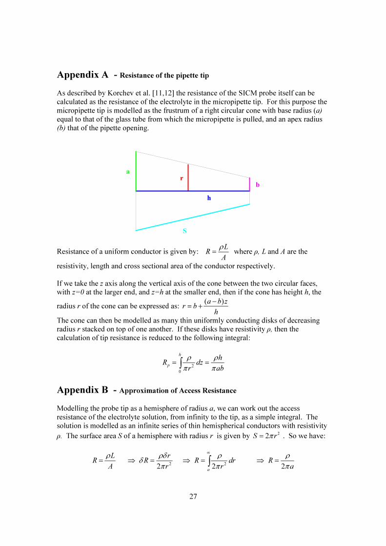
Appendix A - Resistance of the pipette tip As described by Korchev et al. [11,12] the resistance of the SICM probe itself can be calculated as the resistance of the electrolyte in the micropipette tip. For this purpose the micropipette tip is modelled as the frustrum of a right circular cone with base radius (a) equal to that of the glass tube from which the micropipette is pulled, and an apex radius (b) that of the pipette opening.

a

b

h

r

S Resistance of a uniform conductor is given by: LR

Aρ

= where ρ, L and A are the resistivity, length and cross sectional area of the conductor respectively. If we take the z axis along the vertical axis of the cone between the two circular faces, with z=0 at the larger end, and z=h at the smaller end, then if the cone has height h, the radius r of the cone can be expressed as: ( )a b zr b

h−

= + The cone can then be modelled as many thin uniformly conducting disks of decreasing radius r stacked on top of one another. If these disks have resistivity ρ, then the calculation of tip resistance is reduced to the following integral:

20

h

phR dz

r abρ ρ

π π= =∫

Appendix B - Approximation of Access Resistance Modelling the probe tip as a hemisphere of radius a, we can work out the access resistance of the electrolyte solution, from infinity to the tip, as a simple integral. The solution is modelled as an infinite series of thin hemispherical conductors with resistivity ρ. The surface area S of a hemisphere with radius r is given by 22S rπ= . So we have: 2 22 2 2

a

L rR R R dr RA r r aρ ρδ ρ ρδ π π π

∞

= ⇒ = ⇒ = ⇒ =∫

28

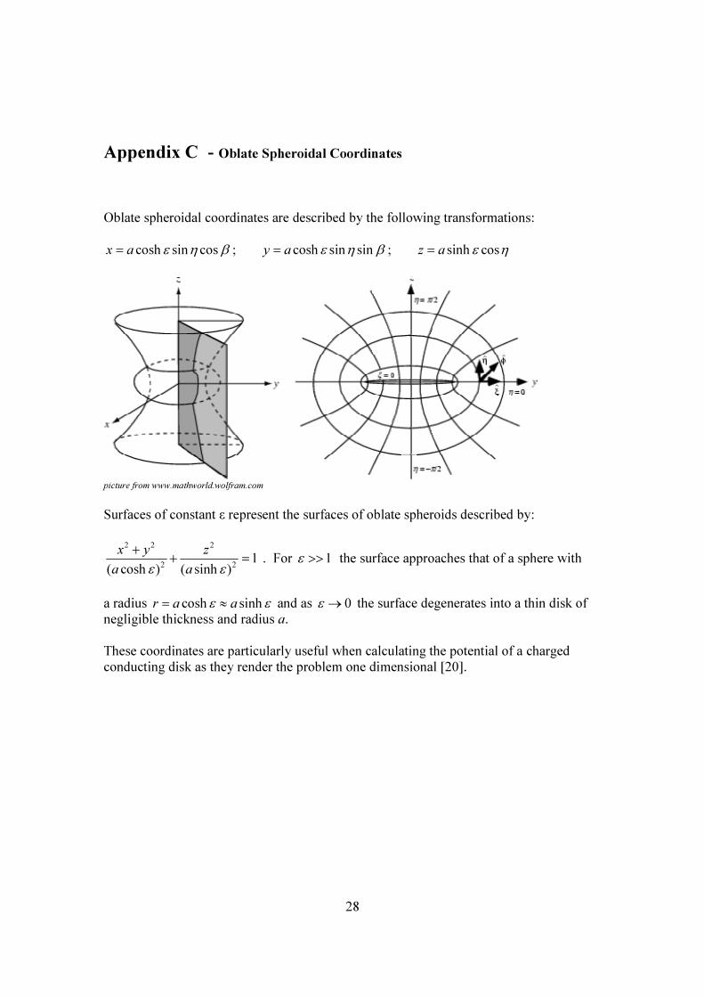
Appendix C - Oblate Spheroidal Coordinates Oblate spheroidal coordinates are described by the following transformations:

cosh sin cos ; cosh sin sin ; sinh cosx a y a z aε η β ε η β ε η= = =

picture from www.mathworld.wolfram.com Surfaces of constant ε represent the surfaces of oblate spheroids described by:

2 2 2

2 2 1( cosh ) ( sinh )x y za aε ε

++ = . For 1ε >> the surface approaches that of a sphere with

a radius cosh sinhr a aε ε= ≈ and as 0ε → the surface degenerates into a thin disk of negligible thickness and radius a. These coordinates are particularly useful when calculating the potential of a charged conducting disk as they render the problem one dimensional [20].

29

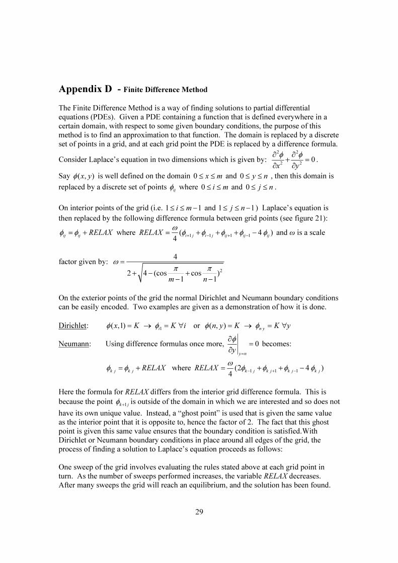
Appendix D - Finite Difference Method The Finite Difference Method is a way of finding solutions to partial differential equations (PDEs). Given a PDE containing a function that is defined everywhere in a certain domain, with respect to some given boundary conditions, the purpose of this method is to find an approximation to that function. The domain is replaced by a discrete set of points in a grid, and at each grid point the PDE is replaced by a difference formula. Consider Laplace’s equation in two dimensions which is given by:

2 2

2 2 0x yφ φ∂ ∂+ =

∂ ∂.

Say ( , )x yφ is well defined on the domain 0 x m≤ ≤ and 0 y n≤ ≤ , then this domain is replaced by a discrete set of points ijφ where 0 i m≤ ≤ and 0 j n≤ ≤ . On interior points of the grid (i.e. 1 1i m≤ ≤ − and 1 1j n≤ ≤ − ) Laplace’s equation is then replaced by the following difference formula between grid points (see figure 21): ij ij RELAXφ φ= + where 1 1 1 1( 4 )4 i j i j ij ij ijRELAX ω φ φ φ φ φ+ − + −= + + + − and ω is a scale

factor given by:

2

42 4 (cos cos )1 1m n

ωπ π

=

+ − +− −

On the exterior points of the grid the normal Dirichlet and Neumann boundary conditions can be easily encoded. Two examples are given as a demonstration of how it is done. Dirichlet: 1( ,1) ix K K iφ φ= → = ∀ or ( , ) n yn y K K yφ φ= → = ∀ Neumann: Using difference formulas once more, 0

y nyφ

=

∂ =∂

becomes:

k j k j RELAXφ φ= + where 1 1 1(2 4 )4 k j k j k j k jRELAX ω φ φ φ φ− + −= + + − Here the formula for RELAX differs from the interior grid difference formula. This is because the point 1k jφ + is outside of the domain in which we are interested and so does not have its own unique value. Instead, a “ghost point” is used that is given the same value as the interior point that it is opposite to, hence the factor of 2. The fact that this ghost point is given this same value ensures that the boundary condition is satisfied.With Dirichlet or Neumann boundary conditions in place around all edges of the grid, the process of finding a solution to Laplace’s equation proceeds as follows: One sweep of the grid involves evaluating the rules stated above at each grid point in turn. As the number of sweeps performed increases, the variable RELAX decreases. After many sweeps the grid will reach an equilibrium, and the solution has been found.

Documents

An attempt to model ion conductance when a SICM approaches a