OPERATIONS RESEARCHVol. 00, No. 0, Xxxxx 0000, pp. 000–000

issn 0030-364X |eissn 1526-5463 |00 |0000 |0001

INFORMSdoi 10.1287/xxxx.0000.0000

c© 0000 INFORMS

An Asymptotically Efficient Mechanism forCombinatorial Network Markets

Rahul JainEE & ISE Departments, University of Southern California, Los Angeles, CA 90089. Email: rahul.jain@usc.edu

Pravin VaraiyaEECS Department, University of California, Berkeley, CA 94720. Email: varaiya@eecs.berkeley.edu

Abstract: We consider the problem of efficient mechanism design for multilateral trading of multiple network

goods with independent private types for players and incomplete information among them. The problem is

motivated by an efficient resource allocation problem in communication networks where there are both buyers

and sellers. In such a setting, budget balance and ex post individual rationality are key requirements, while

efficiency and incentive compatibility are desirable goals. Such mechanisms are difficult, if not impossible

to design. We propose a combinatorial market mechanism which is budget-balanced and ex post individual

rational by design. For a single good with complete information, it is a Nash implementation and efficient. In

fact, we can show that under a “weak rationalizability” assumption, every Nash equilibrium is efficient. Under

incomplete information, the mechanism is budget-balanced, ex post individual rational and asymptotically

efficient and Bayesian incentive compatible. With multiple goods, we establish that with a large number of

players, modelled as a continuum, the auction outcome is a competitive equilibrium.

Key words : Network Resource Allocation, Mechanism Design, Combinatorial Auctions, Double Auctions,

Bayesian-Nash Equilibria. OR/MS subject classification: Games/group decisions: Bidding/auctions,

Natural resources: Energy, Communications.

Area of Review: Environment, Energy, and Natural Resources

History : Submitted: November 13, 2011

1. Introduction

We study a multilateral trading problem with multiple indivisible goods and independent private

types in which ex post budget-balance is required. The problem is partly motivated by the need to

design mechanisms for efficient resource allocation or exchange between strategic internet service

providers such as AT&T and Time-Warner Cable who lease transmission capacity (or bandwidth)

1

to form desired routes and networks and carriers such as Verizon and L3 who own capacity on

individual links. Bandwidth is traded in discrete amounts, say multiples of 100 Mbps, and hence

is an indivisible good. Thus, the buyers want bandwidth on combinations of several links available

in multiples of some indivisible unit. This makes the problem combinatorial. We consider the

interaction in several settings. (Similar problems also occur in other settings such as electricity

markets (Quintero 2001) and spectrum auctions (Milgrom 2000).)

We propose a ‘combinatorial sellers’ bid double auction’ (c-SeBiDA) mechanism for such settings

that achieves a socially desirable interaction among strategic agents. The mechanism is combina-

torial since buyers make bids on combinations of goods, such as several links that form a route.

However, each seller offers to sell only a single type of good (e.g., bandwidth on a single link). We

focus on single-unit demand and supply functions and bids. The mechanism mimics a competitive

market: it accepts buy and sell bids, solves a mixed-integer program that matches bids to maximize

the social surplus, and announces prices at which the matched (i.e., accepted) bids are settled.

The settlement price for a good is the highest price asked by a matched seller (hence “sellers’ bid”

auction). As a result there is a uniform price for each good.

It is shown that in the single good SeBiDA auction game with complete information, a Nash

equilibrium (NE) exists; it is not generally a competitive equilibrium, nor is it unique. Nevertheless,

there is an allocatively efficient NE wherein it is a weakly dominant strategy for all buyers and

for all sellers except the matched seller with the highest-ask price to be truthful. Moreover, every

NE in weakly rationalizable strategies (defined in section 3) is efficient in the single good case. In

the combinatorial case, it is shown through counterexamples that though a NE may not exist, but

when one with trade in every good exists, then every such NE is efficient.

When players have incomplete information, following Harsanyi (1967), we consider the Bayesian-

Nash equilibrium of the auction game. We show that with only a single good, if the players are

“risk-averse” and only use ex post individual rational (IR) strategies (Mas-Collel, et al. 1995), the

semi-symmetric Bayesian-Nash equilibrium strategies (wherein all sellers selling the same good use

2

the same strategy) converge to truth-telling as the number of players becomes very large. Bayesian-

Nash analyses of combinatorial auctions end up being quite intractable, and thus we investigate

the auction with a large number of players (modelled as a continuum economy) and show that the

outcome is a competitive equilibrium.

Previous Work and Our Contribution. The k-double auction was introduced by Chatterjee

and Samuelson (1983) as a model of bilateral bargaining. It was shown by Myerson and Satterth-

waite (1983) that when there is incomplete information, there exists no bilateral mechanism which

is Bayesian incentive compatible (BIC), interim individual rational (IIR), budget-balanced and

efficient. Thus, the notion of “constrained incentive efficiency” was considered by Wilson (1985).

The k-double auction mechanism was further generalized to the single-good multilateral case by

Satterthwaite and Williams (1989a,b). In this paper, we propose a multilateral trading mechanism

for multiple objects. It may be considered to be a generalization and modification of the k-double

auction mechanism (please see remark 1 and example 2 in section 2 for similarities and differences).

A survey of the vast auction theory literature is provided in Klemperer (1999), de Vries and Vohra

(2003), Krishna (2002). Many are extensions of Vickrey’s ideas (Vickrey 1961). A generalization

of the VCG mechanism with participation costs for multi-dimensional types and multiple objects

was introduced in Krishna and Perry (1998). Also, Dasgupta and Maskin (2000) extends the

VCG mechanism to the case of common values, and shows it is constrained efficient. Some multi-

round ascending bid auctions (Ausubel and Milgrom 2002, Perry and Reny 1999) achieve the same

outcome as VCG. However, these are single-sided auction mechanisms. A Vickrey double auction

mechanism for single goods is proposed in Yoon (2001) but it is neither (ex post) budget-balanced

nor individual rational. It appears very difficult to achieve ex post budget balance (along with

efficiency and individual rationality) in double-sided auction mechanisms (Parkes, et al., 2001).

Our interest is in a double-sided auction mechanism for multiple goods with independent private

types (and quasi-linear utility functions). We propose a combinatorial double auction mechanism

which is individual rational and budget-balanced by design, makes a compromise on incentive-

compatibility (IC) and yet is efficient. It is a non-VCG-type double-sided auction mechanism for

3

multiple goods. Like the proposal in Babaioff and Walsh (2005), our mechanism is also NP-hard.

But the mechanism’s mixed-integer linear program structure makes the computation manageable

for many practical applications (Kaskiris, et al. 2007).

The interplay between economic, game-theoretic and computational issues has sparked inter-

est in algorithmic mechanism design (Ronen 2000, de Vries and Vohra 2003). The generalized

Vickrey auction mechanisms for multiple heterogeneous goods are not computationally tractable

(Parkes 2001, Parkes, et al., 2001). Thus, mechanisms that rely on approximation of the inte-

ger program (Parkes 2001, Sandholm 2002), or linear programming (Bikhchandani, et al. 2001)

have been proposed. The results here also relate to the efforts in the network pricing literature

(MacKie-Mason and Varian 1995). There is an ongoing effort to propose mechanisms for divisible

resource allocation in networks through auctions (Yang and Hajek 2007, Jain and Walrand 2010)

and to understand the worst case Nash equilibrium efficiency loss of such mechanisms when users

act strategically (Johari and Tsitsiklis 2004). Optimal mechanisms for single divisible goods that

minimize this efficiency loss have been proposed (Yang and Hajek 2007) though not extended to

the incomplete information case nor for multiple goods. Most of this literature regards the good

as divisible, with complete information for all players. The case of combinatorial bids on multiple

indivisible goods or incomplete information case is harder. The work closest to this paper is Chu

and Shen (2008) which proposes a truthful double auction mechanism for multiple goods with a

“single output restriction”, i.e., each sellers produces at most one unit of a good. It was shown that

the mechanism they propose is strategy-proof, ex post IR, but only ex post weakly budget-balanced.

Moreover, the mechanism is analyzed in the complete information setting alone. No analysis, or

claims are presented for the incomplete information setting. In contrast, we are able to achieve ex

ante (strong) budget-balance. Moreover, we establish efficiency in the complete information setting,

and asymptotic efficiency in the incomplete information setting.

The results in this paper are significant from several perspectives. In the theory of mechanism

design, the VCG class of mechanisms is one of the few positive results (Green and Laffont 1979).

The generalized Vickrey auction (GVA) (with complete information) is ex post individual rational,

4

dominant strategy incentive compatible and efficient. It is however not budget-balanced. With

incomplete information, the expected externality (dAGVA) mechanism (Arrow 1979, d’Aspremont

and Gerard-Varet 1979) is Bayesian incentive compatible, efficient and budget-balanced. It is,

however, not ex post individual rational. Indeed, in the complete information setting there can be

no mechanism that is efficient, budget-balanced, ex post individual rational and dominant strategy

incentive compatible (Hurwicz (1975) impossibility theorem). In the incomplete information setting

there is no mechanism which is efficient, budget-balanced, ex post individual rational and Bayesian-

IC (Myerson and Satterthwaite (1983) impossibility theorem).

In this paper, we provide a combinatorial (market) mechanism which in the single-good com-

plete information case is budget-balanced, ex post individual rational, a Nash implementation and

efficient. In fact, we can show that when players use weakly rationalizable strategies, every Nash

equilibrium is efficient. With multiple goods, a Nash equilibrium may not exist. Nevertheless, we

can establish that when a Nash equilibrium with trade for every good exists, then every such

Nash equilibrium is efficient. Under incomplete information with a single good, the mechanism

s budget-balanced, ex post individual rational and asymptotically Bayesian incentive compatible

and efficient. Thus, the mechanism achieves budget-balance and ex post individual rationality by

design but compromises on incentive compatibility, only achieving asymptotic Bayesian incentive

compatibility and efficiency. With multiple goods and a large number of players, we establish that

the auction outcome is a competitive equilibrium.

The proposed mechanism for multiple heterogeneous goods is related to the (Myerson and Sat-

terthwaite 1983) mechanism for a single good. A positive result is achieved: While it is impossible

to achieve Bayesian incentive compatibility and efficiency along with ex post budget balance and

ex post individual rationality, it is possible to achieve these properties asymptotically even in a

multilateral, multiple goods trading environment.

The rest of this paper is organized as follows. In Section 2 we present the combinatorial seller’s bid

double auction (c-SeBiDA) mechanism. In Section 3 we consider Nash equilibrium of the complete

information auction game, first with a single good and then with multiple goods in a combinatorial

5

setting. Section 4 presents Bayesian-Nash analysis of the incomplete information setting. In Section

5, we investigate c-SeBiDA in a continuum economy model, and show that the auction outcome is

a competitive equilibrium. Section 6 presents some applications.

2. The Combinatorial Sellers’ Bid Double Auction

A buyer places buy bids for a bundle of goods. A buyer’s bid is combinatorial: he must receive all

goods in his bundle or nothing. A buy-bid consists of a buy-price for a single unit of the bundle.

On the other hand, each seller makes non-combinatorial bids. A sell-bid consists of an ask-price to

supply a single unit of the good offered for sale.

The mechanism collects all announced bids, matches a subset of these to maximize the ‘surplus’

(equation (1), below) and declares a settlement price for each good at which the matched buy and

ask bids—which we call the winning bids—are transacted. This constitutes the payment rule. As

will be seen, each matched buyer’s buy bid is larger, and each matched seller’s ask bid is smaller

than the settlement price. There is an asymmetry: buyers make multi-good combinatorial bids, but

sellers only offer one type of good. This yields uniform settlement prices for each good.

In the combinatorial sellers’ bid double auction (c-SeBiDA), each player places only one bid.

c-SeBiDA is a ‘double’ auction because both buyers and sellers bid; we call it a ‘sellers’ bid’ auction

because the settlement price depends only on the matched sellers’ bids.

Formal mechanism. There are L goods indexed 1, · · · ,L, m buyers and n sellers. Buyer i has

(true) reservation value vi for a single unit of a bundle of goods Ri ⊆ {1, · · · ,L}, and submits a

buy bid of bi for one unit of the bundle Ri. We assume that the buyers have quasi-linear utility

functions of the form ubi(x;ω,Ri) = vi ·x+ω where ω is money and x∈ {0,1}. Each seller sells only

one of the L goods. Seller j sells a good lj, has (true) per unit cost cj and offers to sell up to a

single unit of lj at a unit price of aj. Note that there may be many sellers j, j′, etc., selling the

same good lj = lj′ = l, etc. We assume that the sellers also have quasi-linear utility functions of the

form usj(y;ω, lj) =−cj · y+ω where ω is money and y ∈ {0,1}.

The mechanism receives all these bids, and matches some buy and sell bids. The possible matches

6

are described by xi, yj ∈ {0,1}. The mechanism determines the allocation (x∗, y∗) as the solution

of the surplus maximization problem

SMP: maxx,y

∑i bixi−

∑j ajyj (1)

s.t.∑

j yjI(l= lj)−∑

i xiI(l ∈Ri)≥ 0,∀l ∈ [1 :L],

xi ∈ {0,1},∀i, yj ∈ {0,1},∀j,

where I(·) denotes the indicator function. The settlement price is the highest ask-price among

matched sellers,

pl = max{aj : y∗j > 0, l= lj}. (2)

The payments are determined by these prices. If no seller of good l is matched, i.e., good l is not

traded, the price of pl is unspecified. Matched buyers pay the sum of the prices of goods in their

bundle; matched sellers receive a payment equal to the number of units sold times the price for

the good. Unmatched buyers and sellers do not get any allocation and do not make or receive any

payments. This completes the mechanism description.

If i is a matched buyer (x∗i > 0), it must be that his bid bi ≥∑

l∈Ripl; for otherwise, the surplus

(1) can be increased by eliminating the corresponding matched bid. Similarly, if j is a matched

seller (y∗j > 0), and l= lj, his bid aj ≤ pl, for otherwise the surplus can be increased by eliminating

his bid. It is easy to understand how the mechanism picks matched sellers. For each good j, a seller

with lower ask bid will be matched before one with a higher bid. So sellers with bid aj < pl sell.

On the other hand, because their bids are combinatorial, the matched buyers can be determined

only by solving the SMP.

Example 1. Consider one good, three buyers each of whom wants one unit and three sellers

each of whom has one unit to offer. Suppose buyers bid b1 = 3.1, b2 = 2.1, b3 = 1.1 and sellers bid

a1 = 1, a2 = 2, a3 = 3. Then, the revealed social surplus in SMP (1) is maximized when buyers 1 and

2, and sellers 1 and 2 are matched. The price then is p= 2. Note that if bids of buyer 3 and seller

3 are also accepted, this will result in a lower revealed social surplus.

7

Remarks. 1. The single good version SeBiDA resembles the k-double auction (a special case being

called the buyer’s bid double auction (Satterthwaite and Williams 1989b,a, Williams 1991)). The

k-DA is defined as follows: Sellers submit offers aj, j = 1, · · · , n and buyers bids bi, i = 1, · · · , n.

To determine who trades, list these offers/bids as s(1) ≤ s(2) ≤ · · · ≤ s(2n) where s(l) denotes the

lth order-statistic. Thus, s(n) could either be a buy-bid or a sell-offer. Then, for given k ∈ [0,1],

pick price to be p(k) = (1−k)s(n) +ks(n+1). Sell-offers below p and buy-bids above p are accepted.

Others are not. For the special case of k = 1, the k-DA mechanism is the same as the buyer’s bid

double auction (BBDA) mechanism (Satterthwaite and Williams 1989a). The “sell-side version”

would take k= 0 with p= s(n). But note that despite similar nomenclature and spirit, BBDA and

c-SeBiDA determine prices differently. We illustrate the difference through an example.

Example 2. Consider one good, three buyers each of whom wants one unit and three sellers

each of whom has one unit to offer. Suppose buyers bid b1 = 6.1, b2 = 3.1, b3 = 1.1 and sellers bid

a1 = 2, a2 = 4, a3 = 5. (i) BBDA: Then, s(3) = 3.1 and s(4) = 4, and the price determined by BBDA

is p = 4 with one trade between buyer 1 and seller 1. The “sell-side” version of BBDA would

determine a price p= 3.1 with a single trade. k-DA determines a price p ∈ [3.1,4]. (ii) c-SeBiDA:

The mechanism proposed in this paper, on the other hand, determines one trade between buyer 1

and seller 1 with price p= 2.

Thus, the mechanism proposed in this paper is distinct from BBDA (Satterthwaite and Williams

1989b). It is not clear what a generalization of the k-double auction or BBDA would be to the

combinatorial case.

2. The ties between players can be broken by randomly picking the winners. This has no effect on

the auction’s outcome, or its properties unlike other mechanisms.

Our goal is to understand the efficiency and incentive-compatibility properties of the mechanism.

3. Complete Information Nash Equilibrium Analysis of c-SeBiDA

As a first step, we study these properties under complete information. We will assume that players

don’t strategize over the bundles Ri, which will be considered given. A strategy for buyer i is a

8

buy bid bi, a strategy for seller j is an ask bid aj. Let θ denote a collective strategy. Given θ,

the mechanism determines the allocation (x∗, y∗) and the prices {pl}. So the payoff to buyer i and

seller j is, respectively,

ubi(θ) = vi ·x∗i −x∗i ·∑l∈Ri

pl, and usj(θ) = y∗j · plj − cj · y∗j . (3)

The bids bi, aj may be different from the true valuations vi, cj, which however figure in the payoffs.

A collective strategy θ∗ is a Nash equilibrium if no player can increase his payoff by unilaterally

changing his strategy (Fudenberg and Tirole 1991). Define social welfare function for the auction

game as

S(x, y) =∑i

vixi−∑j

cjyj.

where (x, y) satisfy the feasibility conditions of SMP (1). An auction mechanism will be called

efficient if every Nash equilibrium allocation maximizes social welfare.

We say that a strategy bi is weakly dominated for player i if there exists a strategy bi of player i

such that

ui(bi, b−i)≥ ui(bi, b−i),∀b−i

with strict inequality for at least one b−i, where b−i are the strategies of the other players. Such

strategies can be considered as unlikely to be played. Strategies which are not weakly dominated

will be called undominated. Strategies which remain undominated after iterated elimination of

weakly dominated strategies will be called weakly rationalizable strategies (Fudenberg and Tirole

1991).

3.1. Single-good Case

We first consider the single good case and construct a Nash equilibrium which yields an efficient

allocation. We then show that when players play weakly rationalizable strategies, all resulting Nash

equilibria are efficient in the single good case. Without loss of generality, we assume that true

valuations and costs lie in [0,1]. To avoid trivial cases of non-uniqueness, assume all buyers/sellers

have different valuations/costs.

9

Theorem 1 (SeBiDA Auction). (i) A Nash equilibrium (b∗, a∗) exists in the single good

SeBiDA game wherein except for the matched seller with the highest bid on each good, each player

bids truthfully. (ii) Furthermore, any Nash equilibrium in weakly rationalizable strategies has an

efficient allocation.

The proof involves enumerative analysis and can be found in the appendix.

Remarks. 1. It is obvious that even if the efficient allocation is unique, the efficient Nash equilib-

rium need not be unique. Furthermore, there are Nash equilibria where buyers may not bid their

true valuation.

Example 3. Consider the setting of Example 1. Let the bids be a1 = 2.05, a2 = 2.05, a3 = 3, b1 =

2.05, b2 = 2.05 and b3 = 1.1. It is easy to check this is a Nash equilibrium with efficient allocation.

But note that buyer 2 does not bid true valuation. Thus, in SeBiDA it is not a dominant-strategy

for buyers or sellers to be truthful.

2. We have considered Nash equilibrium in weakly rationalizable strategies since it is not rational

for players to play weakly dominated strategies. However, if we do consider all strategies, there

are no-trade Nash equilibria (even in the combintorial setting) which may not be efficient as the

following examples show.

Example 4. Consider a buyer with v= 0.7 and a seller with c= 0.3. Clearly a trade is possible and

in fact any b∗ = a∗ ∈ [0.3,0.7] is a Nash equilibrium with an efficient outcome. However, consider

the bids b= 0 and a= 1. Clearly, this is a Nash equilibrium with no trade, which is inefficient. But,

these strategies are strictly dominated by other strategies, e.g., the buyer can bid anything above

0.3 and the seller anything below 0.7.

Example 5. Consider a two goods (A and B) case. There is one buyer with v = 0.7 for one unit

of both goods, and zero otherwise. There is one seller who offers good A and has c1 = 0.2 and

another seller who offers good B and has c2 = 0.3. Clearly, the efficient allocation involves an

exchange between these players. Now, consider b= 0.6, a1 = 0.4 and a2 = 0.5. It is a no-trade Nash

equilibrium.

10

3. We note that under assumption of weak rationalizability, the inefficient no trade Nash equilibria

(i.e., when a trade is clearly possible) are eliminated from the set of Nash equilibria. However,

in other situations, no trade itself may be the efficient solution. For example, when say there is

a single buyer and a single seller and v < c, there should be no trade. In this case, the no trade

equilibrium is not eliminated under weak rationalizability assumption.

3.2. Combinatorial Case

In the combinatorial case, a Nash equilibrium may fail to exist, even when the efficient allocation

involves trade of every good, as the following example shows.

Example 6. Consider three goods, one seller with one unit for each good. Let there be four buyers.

Buyer 1 wants goods A and B and has v1 = 4, buyer 2 wants A and C and has v2 = 2, buyer 3

wants B and C, and has v3 = 2, and buyer 4 wants C and has v4 = 0.5. There are three sellers with

zero cost, one of each good. It is easy to verify that the efficient allocation is x∗ = (1,0,0,1) and

y∗ = (1,1,1). However, it can be checked that there is no Nash equilibrium in the c-SeBiDA game

for this setting.

Nevertheless, we can show that when there does exist Nash equilibria that involve trade of every

good, then every such Nash equilibrium has to be efficient. Thus, the properties achieved by the

c-SeBiDA mechanism are weaker in the combinatorial case than in the single good case.

Theorem 2. In the combinatorial case, if there exists a Nash equilibrium with non-zero trade for

each good, then every such Nash equilibrium (i.e., with non-zero trade for each good) is efficient.

The proof involves enumerative analysis and can be found in the appendix. It mostly follows ideas

as in the single good case. But there are some notable difficulties due to the combinatorial/bundle

nature of the problem. At times, these can be resolved by introducing a notion of “residual”

valuations and bids on a good. Furthermore, the key is Proposition 1, which is an interesting

observation in its own right.

11

Remarks. 4. When a Nash equilibrium with non-zero trade for every good exists, every such Nash

equilibrium is efficient. However, there can still be inefficient Nash equilibria where there may not

be trade for every good as the following example shows.

Example 7. Consider three goods A, B and C. There are two buyers, the first wants one unit of

(A,B), while the second wants one unit of (B,C). Let v1 = v2 = 1. There is one seller each of A and

C, and two of B, each with cost ci = 0. Then, the optimal allocation is that all match. A Nash

equilibrium is that both buyers bid 1 while all sellers bid 0.5, which is efficient and involves trade

for every good. Now, consider b1 = 1, b2 = 0, sellers of goods A and B bid 0.5 each, but seller of C

bids 1. This is also a Nash equilibrium that is inefficient, and there is no trade for every good.

4. SeBiDA is Asymptotically Bayesian Incentive Compatible

We now consider the incomplete information case. We analyze the SeBiDA market mechanism in

the limit of a large number of players. We assume that the number of buyers and the number of

sellers is the same, n≥ 2. The results can be extended to the case when the number of buyers and

sellers are different.

We will consider a Bayesian game to model incomplete information. Suppose nature draws

c1, · · · , cn from probability distribution U1 and draws v1, · · · , vn from probability distribution U2,

which are such that the corresponding pdfs u1 and u2 have full support on [0,1]. Each player

is then told his own valuation or cost. It is common information that the seller costs are drawn

from U1 and buyer valuations are drawn from U2. Let αj : [0,1]→ [0,1] denote the strategy of the

seller j and βi : [0,1]→ [0,1] denote the strategy of the buyer i. Then, the payoff received by the

buyers and sellers is as defined by equations (3) and (4). Let θ = (α1, · · · , αn, β1, · · · , βn) denote

the collective strategy of the buyers and the sellers. A buyer i chooses strategy βi to maximize

E[ubi(θ);βi], the conditional expectation of the payoff given its strategy βi. The seller j chooses

strategy αj to maximize E[usj(θ);αj], the conditional expectation of the payoff given its strategy

αj. The Bayesian-Nash equilibrium of the game is then the Nash equilibrium of the Bayesian game

defined above.

12

We consider symmetric Bayesian-Nash equilibria, i.e., equilibria where all buyers use the same

strategy β and all sellers use the same strategy α. Let α(c) := c and β(v) := v denote the truth-

telling strategies. Under strategies α and β, we denote the distribution of ask-bids a and buy-bids

b as F and G respectively. We denote [1−F (x)] by F (x). Under α and β, F =U1 and G=U2. We

consider only those bid strategies which satisfy the ex post individual rationality constraint, i.e.,

α(c)≥ c and β(v)≤ v. Denote X = {α : α(c)≥ c} and Y = {β : β(v)≤ v}.

We consider single unit bids and assume that a symmetric Bayesian-Nash equilibrium exists.

Theorem 3. Consider the SeBiDA auction game with (α,β)∈X ×Y, i.e., both buyers and sellers

have ex post individual rationality constraint. Let (αn, βn) be a symmetric Bayesian Nash equilib-

rium with n buyers and n sellers. Then, (i) βn(v) = β(v) = v ∀n≥ 2, and (ii) (αn, βn)→ (α, β) in

the uniform topology as n→∞, i.e., SeBiDA is asymptotically Bayesian incentive compatible.

We will first prove two lemmas.

Lemma 1. Consider the SeBiDA auction game with n buyers and n sellers. Suppose the sellers use

bid strategy α with f(a), the pdf of its ask-bid under strategy α. Then, the best-response strategy of

the buyers βn satisfies βn(v)≥ v for all n≥ 2.

The proof can be found in the appendix. The above conclusion at first glance seems surprising.

A buyer’s strategy is to bid more than his true value. However, intuitively it makes sense for this

mechanism since the prices are determined by the sellers’ bids alone, and by bidding higher, a

buyer only increases his probability of being matched. Of course, if he bids too high, he may end

up with a negative payoff. Result implies that under the ex post individual rationality constraint,

the buyer always uses the strategy βn = β.

Now, we look at the best response strategy of the sellers when the buyers bid truthfully.

Lemma 2. Consider the SeBiDA auction game with n buyers and n sellers and suppose buyers bid

truthfully, i.e., βn = β, and let αn be the sellers’ best-response strategy. Then, (αn, β)→ (α, β) as

n→∞.

13

The proof can be found in the appendix. The conclusion of this Lemma is what we would expect

intuitively. If all buyers bid truthfully, then as the number of sellers increases, increased competition

forces them to bid closer and closer to their true costs.

Proof: (Theorem 3) By Lemma 1 when the sellers use strategy αn, the buyers under the ex post

individual rationality constraint use strategy β. By Lemma 2, when the buyers bid truthfully,

sellers’ best-response is αn. Thus, (αn, β) is a Bayesian-Nash equilibrium with n players on each

side of the market. Further, Lemma 2 shows that (αn, βn) = (αn, β)→ (α, β) as n→∞, which is

the conclusion we wanted to establish.

Thus, under the ex post IR constraint, SeBiDA is ex ante budget balanced, asymptotically

Bayesian incentive compatible and efficient. Unlike in the complete information case when the

mechanism is not incentive compatible, yet the outcome is efficient, in the incomplete information

case, the mechanism is only asymptotically efficient.

The mechanism proposed in this paper is related to the buyer’s bid double auction (BBDA)

mechanism (Satterthwaite and Williams 1989a,b, Williams 1991). While the spirit of the two

mechanisms is the same (maximizing the efficiency of trading), the prices and the payments are

different. In SeBiDA, the prices are determined by the bids of the sellers only. This makes the

market asymmetric: In the complete information case, all buyers have no incentive to bid non-

truthfully but at least one seller does.

In BBDA, the determined price could be either a buyer’s bid or a seller’s bid. In Williams (1991),

it is simply assumed that the buyers bid truthfully which need not be true (Satterthwaite and

Williams 1989b). In fact we found that for SeBiDA, even though under complete information it is

a dominant strategy for buyers to bid truthfully, this is not the case for incomplete information.

The proof techniques used in this paper are in part inspired by those developed by Chatterjee and

Samuelson (1983), Satterthwaite and Williams (1989a,b), Williams (1991). The rate of convergence

of SeBiDA can be obtained from the analysis in the proof of Lemma 2. Though, Nash equilib-

rium analysis was ignored in (Satterthwaite and Williams 1989b). Finally, the ex post individual

14

rationality constraint seems restrictive at first glance. However, in two human subject experiments

we have conducted using this mechanism, it was observed that all subjects in fact always used

strategies that were ex post individual rational (Kaskiris, et al. 2007). Thus, the predictive power

of the result does not seem diminished in real-world settings despite the assumption made. It is also

pertinent to mention (Satterthwaite and Williams 2002) wherein the authors show that the k-DA

class of market mechanisms are worst-case asymptotic optimal, where optimality is measured in

how quickly the inefficiency diminishes as the market size increases. The mechanisms are evaluated

in the least favorable trading environment.

Bayesian-Nash Equilibrium in a Special Combinatorial Case

We now provide an extension of Theorem 3 to a combinatorial case.

Corollary 1. Suppose the buyer valuations and seller costs are uniform over [0,1], i.e., U1 =

U2 =U [0,1]. The combinatorial demands of buyers are such that each item is demanded by n buyers

and there are n sellers for each item. Then, the claim of Theorem 3 still holds, i.e., if both buyers

and sellers have ex post individual rationality constraint and (αn, βn) is a symmetric Bayesian-Nash

equilibrium, then, (i) βn(v) = β(v) = v ∀n≥ 2, and (ii) (αn, βn)→ (α, β) in the uniform topology

as n→∞, i.e., c-SeBiDA is asymptotically Bayesian incentive compatible.

The reader can check that the arguments in proof of Theorem 3 still hold. We provide an intuitive

argument. Suppose a buyer i would present his combinatorial bid as an itemized bid, i.e., a bid for

each item in his bundle. Now, for each item in its bundle it faces the same number of buyers n− 1

and the same number n of sellers. Suppose all other buyers j 6= i divide their bid equally among

all items in their bundle, i.e., if bj is the bid for the bundle Rj, bj/|Rj| is the bid for each item in

Rj. Then, buyer i has to divide his bid bi among his items in such a way that his expected payoff

is maximized. For given bids of all players, his payoff is zero if he is not matched and non-zero if

he is matched. Thus, he has to itemize his bid in a way that he maximizes the probability of being

matched. It can be verified that when buyer valuations and seller costs are drawn uniform over

15

[0,1], the probability of his bid being accepted is maximum if the bid is divided equally among all

items in his bundle. Thus, he would use the same strategy βn = bj/|Rj| on each item which would

induce the same distribution of buy-bids G on each item. This is true for all buyers since they are

symmetric. Similarly, all sellers will use the same bid strategy αn which will induce the distribution

of ask-bids F . Now, the game has been reduced to a single-item auction game on each item, and

the result follows from Theorem 3.

From the Nash equilibrium analysis for the combinatorial case and the Bayesian-Nash analysis for

the single item case, it seems plausible that the Bayesian-Nash equilibrium result can be extended

to the general combinatorial case. However, the analysis becomes rather messy and intractable.

New ideas are needed to accomplish Bayesian-Nash analysis of combinatorial auctions and will be

accomplished in future work. Thus, in the next section, we show that the c-SeBiDA outcome in

the combinatorial setting, when there are a large number of players (as in a continuum model) is

a competitive equilibrium.

5. c-SeBiDA outcome is a Competitive Equilibrium in a continuum model

We now consider the c-SeBiDA mechanism, and investigate the existence of a competitive equi-

librium (Arrow and Hahn 1971). It can easily be established that a competitive equilibrium may

not exist in such a setting with a finite number of players. We thus investigate the behavior of

the outcome of the c-SeBiDA auction when there are a large enough number of players such that

no single player by itself can affect the outcome. An idealization is a continuum of agents. Such

a setting was first considered by Aumann (1964) in a general equilibrium setting and others have

used this approach to analysis of games (Jackson 1992, Jackson and Manelli 1997).

Assume the continuum of buyers is indexed by t∈ [0,1], and the continuum of sellers is indexed

by τ ∈ [0,1]. There are m types of buyers and n types of sellers. Let B1, · · · ,Bm and S1, · · · , Sn

partition [0,1] so that all buyers in Bi demand the same set of items Ri (corresponding say to a

route), and all sellers in Sj offer the same item lj, Lj = {lj}. We assume that the partitions Bi’s

and Sj’s are subintervals.

16

A buyer t ∈Bi has true value v(t), bids p(t) per unit for the set Ri, and demands δ(t) ∈ [0,D]

units. Suppose v(t), p(t)∈ [0, V ]. A seller τ ∈ Sj has true cost c(τ) and asks q(τ) for the item(s) Lj

with supply σ(τ)∈ [0, S] units, with c(τ), q(τ)∈ [0,C]. Let x(t) and y(τ) be the decision variables,

i.e. buyer t’s x(t) is 1, if his bid is accepted, 0 otherwise. And similarly seller τ ’s y(τ) is 1 if his

offer is accepted, 0 otherwise. We assume that within each partition Bi, the buyers’ bid function

b(t) is non-increasing, and within each partition Sj, the sellers’ bid function q(τ) is nondecreasing.

Note that in this section we will assume that their bundles are all-or-none kind: All demand

must be met or none. Denote the indicator function by I(·) and as before, consider the surplus

maximization problem cLP:

supx,y

∫ 1

0

m∑i=1

x(t)δ(t)p(t)I(t∈Bi)dt −∫ 1

0

n∑j=1

y(τ)σ(τ)q(τ)I(τ ∈ Sj)dτ (4)

s.t.

∫ 1

0

n∑j=1

y(τ)σ(τ)I(l ∈Lj, τ ∈ Sj)dτ −∫ 1

0

m∑i=1

x(t)δ(t)I(l ∈Ri, t∈Bi)dt≥ 0,

∀l ∈ [1 :L] and x(t), y(τ) ∈ {0,1},∀t, τ ∈ [0,1].

The mechanism determines ((x∗, y∗), p) where (x∗, y∗) is the solution of the above continuous linear

integer program and for each l ∈ [1 :L],

pl = sup{q(τ) : y(τ)> 0, τ ∈ Sl}, (5)

pl = inf{q(τ) : y(τ) = 0, τ ∈ Sl}. (6)

The mechanism announces prices p= (p1, · · · , pL); the matched buyers (those for which x∗(t) = 1)

pay the sum of the prices of the items in their bundle while the matched sellers (those for which

y∗(τ) = 1) get a payment equal to the number of their items sold times the price of the item. When

buyers and sellers bid truthfully, the following result holds.

Theorem 4. If the bid function of the sellers q : [0,1]→ [0,C] is continuous and nondecreasing in

each partition Sj of [0,1], then (x∗, y∗) is a competitive allocation and p is a competitive price.

The proof can be found in the appendix. The implication of this result is that as the number of

players becomes large, the outcome of the above auction approximates the competitive equilibria of

17

the associated continuum exchange economy. We will defer discussion of the relationship between

the Nash equilibria and the competitive equilibria to the conclusions section.

We now show that the assumption that the sellers’ bid function is piecewise continuous and

non-decreasing is necessary for the c-SeBiDA’s price to be a competitive price.

Example 8. Suppose that there is only one item. Buyers t∈ [0,0.5] have reservation value 3 while

buyers t ∈ (0.5,1] have reservation value 4. Sellers t ∈ [0,0.5] have reservation cost 5 while sellers

t ∈ (0.5,1] have reservation cost 2. Then, it is clear that the buyers in (0.5,1] and sellers (0.5,1]

will be matched with surplus 0.5× 2 = 1. Thus, p= 2 which is not equal to p= 3. As can be easily

checked, the competitive price is λ∗ = 3 different from p.

6. Other Applications

We now discuss some of the direct applications of the auction mechanism proposed. How the

problem of bandwidth allocation in a communication network can be solved using the

market mechanism has been discussed in the introduction. We now show how some other problems

of resource allocation may also be formulated as combinational markets, and solved using the

mechanism proposed.

Designing Efficient Electric Power Markets. Let us now consider electric power markets.

Assume time [0, T ] to be slotted. Let a buyer i need 1 MW of power in time slot t. (Power in multi-

ple time slots can be bought by making multiple bids). Let his bid be bi(t) when his true maximum

willingness to pay is vi(t). Suppose a seller j offers Q MW of power over the time interval [0, T ].

This is equivalent to a bundle Rj = {(1,Q), · · · , (T,Q)}. And the seller specifies an ask of a for

this bundle. Thus, sellers make combinatorial bids while buyers make non-combinatorial bids. A

mechanism analogous to c-SeBiDA can be used where the buy-bids determine the price of power in

each time slot. In such a mechanism, the sellers will not have any incentive to act strategically and

misreport their true valuation and supply. Furthermore, the mechanism is incentive-compatible

(asymptotically Bayesian-incentive compatible in the incomplete information case), and the result-

ing allocation is efficient.

18

Air-Traffic Control Through Auctions. A typical metro airport handles hundreds of takeoffs

and landings each hour. Often the flights get delayed due to weather or other logistical reasons.

Thus, the air-traffic control has to adjust the landing and takeoff schedules to take into account

such changes. For an airline, a change in takeoff schedule at one airport is also accompanied by a

change in the landing schedule at another. Thus, the changes may occur in combinations, i.e., the

allocation problem is combinatorial. The slot allocation or reallocation problem can be solved in

a distributed manner using an auction mechanism since the players involved (the various airlines)

are self-interested and have their own selfish economic incentives.

Let x = 1, · · · ,N denote the locations and t = 1, · · · , T denote the time-slots on any day. Let

(T,x, t) denote a takeoff slot at location x at time t, and (L,y, s) denote a landing slot at location

y and time s. A buyer airline then would like to buy a bundle R = {(T,x, t), (L,y, s)} of takeoff

and landing slots for a flight taking off from x at time t and landing at y at time s for at most b

when its maximum willingness (or valuation) is v. While a seller airline whose flight R has gotten

rescheduled might want to offer (T,x, t) and (L,y, s) for sale at aT and aL respectively when its

minimum acceptable price (or true cost) might be cT and cL respectively.

Thus, the slot re-allocation problem can be solved using a combinatorial double-sided auction

such as c-SeBiDA. And if c-SeBiDA is used, then by the results of sections 3-5, it would yield an

efficient allocation (asymptotically efficient when there is incomplete information), providing a way

of solving a difficult distributed resource allocation problem.

7. Conclusions

We have introduced a combinatorial, sellers’ bid, double auction (c-SeBiDA). The first result con-

cerned the Nash equilibria for SeBiDA with complete information. In c-SeBiDA, settlement prices

are determined by sellers’ bids. We have shown that in the single good case, a Nash equilibrium

exists and every Nash equilibrium in weakly rationalizable strategies is efficient. Moreover, there

is a Nash equilibrium in undominated strategies wherein truth-telling is a dominant strategy for

all players except the highest matched seller for each good. In the combinatorial case, a Nash

19

equilibrium may not exist. Nevertheless, we showed that when a Nash equilibrium with non-zero

trade for every good exists, every such Nash equilibrium is efficient.

The second result concerned the Bayesian-Nash equilibrium of the market mechanism under

incomplete information. We have shown that under the ex post individual rationality constraint, the

semi-symmetric Bayesian-Nash equilibrium strategies converge to truth-telling. Thus, the mecha-

nism is asymptotically Bayesian incentive compatible, and hence asymptotically efficient.

Thus, we have proposed an combinatorial market mechanism for a multilateral network trading

environment. In such an environment it is impossible to achieve all the four desirable properties

of an auction mechanism. Nevertheless, we have shown that it is still possible to achieve budget

balance and ex post individual rationality, and asymptotic Bayesian incentive compatibility and

efficiency.

In Jain and Varaiya (2004), we considered a more general setting and showed that a competitive

equilibrium exists in a continuum model of an exchange economy with indivisible goods and money

(a divisible good). There, using results from optimal control, we also showed that within the

continuum model, the c-SeBiDA outcome is a competitive equilibrium. This again suggests that in

the finite setting, the auction outcome is close to efficient.

The issue of computational complexity for such mechanisms becomes very important when there

are a large number of players. Similar concerns arise in Babaioff and Walsh (2005) as well. However,

the computational problem here involves solving a boolean linear program, which can be solved

computationally efficiently.

We have tested the proposed mechanism c-SeBiDA through human-subject experiments. They

suggest good performance in laboratory settings, and can be found elsewhere (Kaskiris, et al. 2007).

Finally, while our work was primarily motivated by a market mechanism design problem, it

can also be considered as an indirect contribution to the strategic foundations of competitive

network markets (Gale 2000). Related literature relates Nash and Bayesian-Nash equilibrium with

competitive equilibrium. The basic idea is that as the economy gets large (in our context the

20

number of buyers and sellers and quantities of goods all go to infinity), Nash equilibrium strategies

should converge to competitive equilibrium strategies, because the ‘market power’ diminishes.

The relationship is first investigated in Roberts and Postlewaite (1976). In a later paper (Gul

and Postlewaite 1992), it is shown that under certain regularity conditions, a sufficiently repli-

cated economy has an allocation which is incentive-compatible, individually-rational and ex-post

ε-efficient. Similarly Jackson (1992) shows that the demand functions that an agent might consider

based on strategic considerations converge to the competitive demand functions. Further, Jackson

and Manelli (1997) shows that under certain conditions on beliefs of individual agents, not only

do the strategic behaviors of individual agents converge to the competitive behavior but the Nash

equilibrium allocations also converge to the competitive equilibrium allocation. The formulation in

Wilson (1985) is a buyer’s bid double auction with a single type of good that maximizes surplus. It

is shown that with Bayesian-Nash strategies, the mechanism is asymptotically “incentive efficient,”

the notion of incentive efficiency being different from that of incentive compatibility and efficiency

that we use here. Along a different line of investigation, Gresik and Satterthwaite (1989), Satterth-

waite and Williams (1989b), Rustichini, et al. (1994) investigate the rate of convergence of the Nash

equilibria to the competitive equilibria for buyer’s bid double auction. Finally, implementation and

mechanism design in a setting with a continuum of players is discussed in Mas-Colell and Vives

(1993). We have provided a market mechanism that asymptotically achieves competitive behavior

in multilateral, multiple good trading environment with incomplete information.

Acknowledgements The authors owe thanks to Wenyuan Tang of USC for help in resolving

the proof of Proposition 1, and to Charis Kaskiris for his experimental work (Kaskiris, et al. 2007)

based on this paper that helped to refine the earlier versions of the proposed mechanism. Gratitude

is also owed to Profs. Chris Shannon, Hal Varian and Jean Walrand of UC Berkeley, Bill Zame

of UCLA, John Ledyard of Caltech and Ramesh Johari of Stanford University for many helpful

discussions and valuable feedback.

21

Appendix

Proof of Theorem 1

Proof: (i) We will show existence by construction. Suppose buyer i has reservation value vi and

bids bi, while a seller j has a reservation cost cj and bids aj. Without loss of generality, assume

that v1 ≥ · · · ≥ vM and c1 ≤ · · · ≤ cN . Let k= max{0, i : ci ≤ vi}. If k= 0, denote ak = minj aj.

First consider the case where k= 0, that is there no trade at efficient allocation. In that case, let

aj = cj and bi = vi be the strategies. Since k = 0, it is quite obvious that minj aj >maxi bi. Thus,

no buyer or seller could ensure a match by unilaterally deviating from his strategy. Thus, if no

trade is the efficient allocation, then all players bidding truthfully is a Nash equilibrium.

We now consider the more interesting case of there being a trade at an efficient allocation (k≥ 1).

Consider the following set of strategies: ∀i, bi = vi; ∀j, 6= k,aj = cj; ak = min{ck+1, vk}. The

first k buyers and sellers are matched and the settlement price is p= ak.

Consider a matched buyer i ≤ k. This buyer has no incentive to bid lower, since by doing so

he may be able to lower the price but then he will also become unmatched; since he is already

matched, he has no incentive to bid higher.

Consider an unmatched buyer i > k. Observe that bi = vi < min{bk, ak+1}. Clearly, he has no

incentive to bid lower, as he will remain unmatched. He can become matched by bidding above ak

but then if he does get matched, he will pay ak > vi and his payoff will be negative.

Consider an unmatched seller j > k. He has no incentive to bid higher, as he will remain

unmatched. He can get matched by bidding lower than ak but since his cost is cj > ak, his payoff

will be negative.

Consider a matched seller j < k. By bidding lower, this seller will not improve his payoff. If he

bids higher to increase the settlement price, this will happen only if he bids above ak, but then he

will become unmatched.

Lastly, consider the ‘marginal’ matched seller k. He will not bid lower, as that will decrease his

payoff. If he bids more than ak, his bid will exceed either bk or ak+1, and in either case he will

become unmatched.

22

Thus, the strategies chosen above is a Nash equilibrium which yields the efficient allocation

z∗ = (x∗, y∗), which matches buyers with highest valuation and sellers with least cost.

(ii) We now show that in case of a single good any Nash equilibrium allocation in weakly

rationalizable strategies is efficient. (We will drop the subscript l for sellers).

First, observe that a seller’s bid below his cost is weakly dominated by his bid at cost: Thus,

aj ≥ cj,∀j. Further, since this elimination of strategy space of the sellers is common knowledge, no

buyer will bid below cmin = minj cj.

Let Bmatched and Smatched denote the set of buyers and sellers that are matched at a Nash

equilibrium (b, a). It is worth noting that at an equilibrium, the transaction price p= min{bi : i ∈

Bmatched}= max{aj : j ∈ Smatched}.

Now suppose z := (x, y) is an allocation, corresponding to the Nash equilibrium (b, a), which is

not efficient. There are two main cases:

(A) ‘No Trade is Efficient’ Case: Suppose that the efficient allocation (z∗ := (x∗, y∗)) involves

no trade, but the allocation z does. This implies that vi < cj, ∀i, j but there exists some buyer i

and seller j such that bi ≥ cj. Then, either bi > vi or aj < cj. In both cases, one of the buyer i or

the seller j has an incentive to deviate.

(B) ‘Non-zero Trade is Efficient’ Case: (1) First, suppose that the efficient allocation z∗ involves

a trade but the allocation z involves no trade. Let i∗ denote the buyer with highest value vi and

j∗ denote the seller with the least cost cj (c∗j = cmin). Then, vi∗ ≥ cj∗ but cmin ≤ bi∗ < aj∗ . But

then this cannot be a Nash equilibrium since either the buyer or the seller will have an incentive

to deviate.

(2) Now, suppose that the efficient allocation z∗ involves a trade and the allocation z involves a

trade but is not efficient. Then, the two allocations must differ in one of the following ways as we

go from z∗ to z:

(a) z∗ and z differ only among sellers: A (non-empty) set of sellers Sout matched in z∗, is no

longer matched in z and a (non-empty) set of sellers Sin are now matched;

23

(b) z∗ and z differ only among buyers: A (non-empty) set of buyers Bout matched in z∗, is no

longer matched in z and a (non-empty) set of buyers Bin are now matched;

(c) All buyers and sellers matched in z∗ remain matched in z, and some new buyers Bin and

some new sellers Sin now get matched;

(d) No new buyers and sellers are matched in z and some old buyers Bout and some old sellers

Sout are now not matched;

(e) A set of buyers Bout and a set of sellers Sout are no longer matched and a set of buyers Bin

and a set of sellers Sin are now matched in z.

Now, we establish that in each case, the inefficient allocation cannot be a Nash equilibrium

allocation.

Case (a) Suppose j1 ∈ Sin and j2 ∈ Sout. Then, it must be that cj1 > cj2 but aj1 < aj2 . But then

either j1’s payoff is negative or j2 can also bid just below j1’s bid. In either case z cannot be a

Nash equilibrium allocation.

Case (b) Suppose i1 ∈Bin and i2 ∈Bout. Then it must be that vi1 < vi2 and bi1 > bi2 . But then

either i1’s payoff is negative or i2 can also bid just above i1’s bid. In either case z cannot be a Nash

equilibrium allocation.

Case (c) Denote i := arg maxi∈Binbi and j := arg minj∈Sin aj. Then, vi < cj and bi ≥ aj. But then

at least one of the two has a negative payoff at (b, a), and so will deviate, in which case it cannot

be a Nash equilibrium outcome.

Case (d) Denote i := arg maxi∈Bout vi and j := arg minj∈Sout cj. And denote the transaction price

with bids (b, a) by p. Then, vi ≥ cj and bi < aj. Now, if aj < vi, then clearly, buyer i has an incentive

to bid just above aj and match. Similarly, if bi > cj, then seller j has an incentive to bid just below

bi and match. In either of these cases, the bids under consideration cannot be a Nash equilibrium.

Now, let us consider the case bi ≤ cj ≤ vi ≤ aj. There are three sub-cases: if p ∈ (bi, cj], then

buyer i can raise his bid and match; if p∈ [vi, aj), then seller j can lower his bid and match; and if

p ∈ (cj, ai), then both the buyer i and the seller j have an incentive to deviate from their current

24

bids and match. Thus, in none of the above sub-cases can the bids under consideration be a Nash

equilibrium.

Case (e) Denote i := arg mini∈Binbi and j := arg maxj∈Sin aj, and i := arg maxi∈Bout bi and j :=

arg minj∈Sout aj. And denote the transaction price with bids (b, a) by p. Then, bi ≥ p ≥ aj and

bi ≤ p≤ aj.

Now, observe that vi > vi and cj < cj since players i and j are matched in z∗, the efficient

allocation but players i and j are not. Further, bi ≥ p. So, either vi ≥ p, in which case vi ≥ p as

well and so buyer i can increase his bid to match; or vi < p, in which case buyer i has negative

payoff and so it will decrease his bid. Thus, in either case, the buyer has an incentive to deviate,

and hence the allocation z cannot correspond to a Nash equilibrium. A similar argument can also

be given for sellers.

Thus, for every case above, the corresponding bids cannot be a Nash equilibrium. This proves

claim (ii) of the theorem.

Proof of Theorem 2

Proof: Let Bmatched and Smatched denote the set of buyers and sellers that are matched at a Nash

equilibrium (b, a). Now suppose z := (x, y) is an allocation, corresponding to the Nash equilibrium

(b, a), which is not efficient. Denote the efficient allocation that involves a trade for all goods by

z∗ and the allocation z that also involves a trade for all goods but is not efficient. Then, the two

allocations must differ in one of the following ways as we go from z∗ to z:

(a) z∗ and z differ only among sellers: A (non-empty) set of sellers Sout matched in z∗, is no

longer matched in z and a (non-empty) set of sellers Sin are now matched;

(b) z∗ and z differ only among buyers: A (non-empty) set of buyers Bout matched in z∗, is no

longer matched in z and a (non-empty) set of buyers Bin are now matched;

(c) All buyers and sellers matched in z∗ remain matched in z, and some new buyers Bin and

some new sellers Sin now get matched;

25

(d) No new buyers and sellers are matched in z and some old buyers Bout and some old sellers

Sout are now not matched;

(e) A set of buyers Bout and a set of sellers Sout are no longer matched and a set of buyers Bin

and a set of sellers Sin are now matched in z.

(f) We club all cases into one that do not fall into any of the above five categories.

Case (a) Suppose (l, j1)∈ Sin and (l, j2)∈ Sout. Then, it must be that cl,j1 > cl,j2 but al,j1 < al,j2 .

But then either (l, j1)’s payoff is negative or (l, j2) can also bid just below (l, j1)’s bid. In either

case z cannot be a Nash equilibrium allocation.

Case (b) Now, given the sets of buyers Bin and Bout, let pl denote the set of prices on the links

at the allocation z. Then, it must be that

∑i∈Bout

vi >∑i∈Bin

vi ≥∑i∈Bin

∑l∈Ri

pl.

The first inequality follows because the set of Buyers Bout match ahead of the buyers Bin at the

efficient allocation z∗. The second inequality follows because the buyers Bin are matched with

allocation z and pay prices pl. Now, since (x, y) is the optimal allocation (i.e., auction outcome)

with bids (b, a), it follows that for any feasible allocation (x, y),

∑i

bixi−∑j

aj yj ≥∑i

bixi−∑j

ajyj.

Now, clearly there exists an i∈Bout such that vi >∑

l∈Ripl. Before proceeding further, we establish

a claim that we will use repeatedly in many cases.

Proposition 1. If a buyer i is unmatched at an allocation z with prices p and bids (b, a) and

vi >∑

l∈Ripl, then buyer i has an incentive to deviate.

Proof: Let buyer i be such an unmatched buyer, and define b′i =∑

l∈Ripl + ε for small enough

ε > 0. Consider the bids (b′, a′) such that a′ = a and b′−i = b−i and b′i as defined above. Denote the

allocation with these bids by z′ = (x′, y′).

We claim that the allocation (x′, y′) 6= (x, y). Indeed, consider an allocation z′′ = (x′′, y′′) obtained

from (x, y) in the following manner: For each good l in buyer i’s bundle Ri, at the equilibrium

26

allocation z, either there is an unmatched marginal seller such that al,kl+1 = al,kl = pl (denote the

set of such goods by Ri ⊆Ri), or there is a marginal matched buyer il (say) such that the surplus

of this buyer is zero, i.e., bil =∑

l′∈Rilpl′ (denote the set of such goods by Ri =Ri− Ri). Thus, a

feasible allocation z′′ = (x′′, y′′) can be constructed by matching such a marginal unmatched seller

on good l if it exists, i.e., y′′l,kl+1 = 1, or else dropping the marginal matched buyer with zero surplus,

i.e., x′′il = 0. This means that the allocation z′′ is an improvement over z with bids (b′, a′), i.e.,

∑i

b′ix′′i −∑j

a′jy′′j >

∑i

b′ixi−∑j

a′j yj =∑i

bixi−∑j

aj yj.

The strict inequality follows because the allocation z′′ is a strict improvement over the allocation z

(since only marginal buyers with zero surplus in z are now unmatched, while buyer i with positive

surplus is now matched). The equality follows because xi = 0 and all bids other than b′i are the

same as before. Thus, the allocation must change with bids (b′, a′).

We next claim that buyer i must be matched in allocation z′. Suppose not, then

∑i

bix′i−∑j

ajy′j =∑i

b′ix′i−∑j

a′jy′j ≥∑i

b′ix′′i −∑j

a′jy′′j >

∑i

bixi−∑j

aj yj.

Here, the equality follows because the bids (b′, a′) and (b, a) differ only in buyer i’s bid but x′i = 0

by assumption. The first inequality follows because by definition z′ = (x′, y′) is the auction outcome

with bids (b′, a′) and thus maximizes the surplus. The second strict inequality follows from above.

This would then imply that the allocation z′ is optimal (auction outcome) with bids (b, a).

Now, since buyer i can be matched at bid b′i (as defined earlier), and vi > b′i ≥∑

l∈Rip′l since

buyer i is matched with bids (b′, a′), buyer i has an incentive to deviate from his bid bi.

Thus, (b, a) cannot be a Nash equilibrium in this case.

Case (c) For a fixed l, denote (l, j) := arg min(l,j)∈Sin al,j and let i∈Bin be any such buyer. Then,

vi <∑

l∈Ricl,j since these bidders are not matched at z∗ and bi ≥

∑l∈R

ial,j since they are matched

at z. But then either buyer i or one of the sellers (l, j) with l ∈Ri has a negative payoff at (b, a),

and so will deviate, in which case it cannot be a Nash equilibrium outcome.

27

Case (d) Denote j(l) := arg min(l,j)∈Sout cl,j and i∈Bout, any such buyer. And denote the prices

with bids (b, a) by p. Then, pl ≤ cl,j(l) otherwise any seller (l, j(l)) can outbid the highest matched

seller on l in the allocation z.

Furthermore, vi >∑

l∈Ricl,j(l) and bi <

∑l∈Ri

al,j(l). Now, if∑

l∈Rial,j(l) < vi, then clearly, buyer

i has an incentive to bid just above∑

l∈Rial,j(l) and match.

And if∑

l∈Rial,j(l) ≥ vi >

∑l∈Ri

cl,j(l) ≥∑

l∈Ripl, then by Proposition 1 above, the unmatched

buyer i will deviate by changing his bid to b′i=∑

l∈Ripl + ε for some small enough ε > 0. Conse-

quently, the bids (b, a) cannot be a Nash equilibrium.

Case (e) Denote j(l) := arg max(l,j)∈Sin al,j and j(l) := arg min(l,j)∈Sout al,j, and let i ∈ Bin and

i ∈Bout be any buyers. Let Rii :=Ri ∩Ri be the set of common goods in the bundles of the two

buyers. Denote Rii := Ri \Rii and Rii := Ri \Rii. We shall use the shorthand p(R) to mean the

sum∑

l∈R pl.

Now, first consider the case when there is a common good between sellers Sin and Sout. Then,

clearly as in case (a), the bids under consideration cannot be a Nash equilibrium.

Thus, consider the case when the sellers Sin and Sout do not have any good in common and

suppose that no two buyers i∈Bin and i∈Bout have a good in common, i.e., Rii = ∅. Then, again

this reduces to cases (c) (for Bin, Sin) and (d) (for Bout, Sout) above, and we can conclude that the

bids under consideration cannot be a Nash equilibrium.

Now, we are left with the case where sellers Sin and Sout do not have a good in common and

some buyers i and i do, i.e., Rii 6= ∅. Further, we are given that there is at least one trade for each

good. Thus, clearly

pl ≤ cl,j(l) ≤ p∗l , for l with Sout, (7)

pl ≥ cl,j(l) ≥ p∗l , for l with Sin, (8)

otherwise some sellers would have an incentive to deviate. Further note that

vi−∑l∈Ri

p∗l > vi−∑l∈R

i

p∗l . (9)

28

This implies that

vi− p(Rii)≥ vi− p∗(Rii)≥ vi− p∗(Rii)≥ vi− p(Rii)≥ p(Rii)

which further implies that vi > p(Ri). The first inequality above uses inequality (7), the second

used inequality (9), and the third uses inequality (8). Now, as in case (b), by Proposition 1, bidding

p(Ri) + ε for small enough ε > 0, buyer i can get matched with a positive payoff, and hence has an

incentive to deviate. Thus, (b, a) cannot be a Nash equilibrium in this case.

Cases (f) (Reduction of remaining cases to other cases) It can be easily checked that only the

following cases can feasibly occur.

(i) The cases where Sin, Sout 6= ∅ and either Bin = ∅ or Bout = ∅ but not both, can be reduced to

case (a) above in the following manner. Clearly, if Bin = ∅, then there cannot be any good l on

which there is a new seller in Sin but no seller in Sout. Thus, Sin ⊆ Sout. But then this case reduces

to case (a) as a seller i ∈ Sout can outbid a seller j ∈ Sin on such a good l. Now, if Bout = ∅, then

we can easily conclude that Sout ⊆ Sin, and again this is similar to case (a).

(ii) The cases where Bin,Bout 6= ∅ and either Sin = ∅ or Sout = ∅, but not both can be reduced to

case (b) above in the following manner.

(α) First, consider the case where Sin = ∅ and Sout 6= ∅. Then, by efficiency of the allocation z∗,

we can easily conclude that

∑i∈Bout

vi >∑i∈Bout

vi−∑j∈Sout

cj >∑i∈Bin

vi >∑i∈Bin

∑l∈Ri

pl,

where the second inequality follows because buyers Bout and sellers Sout are matched at the efficient

allocation instead of the buyers Bin. The first inequality is obvious and the third follows in the

same way as in case (b). It can now easily be checked that the rest of the arguments there follow

unchanged, and we cannot have a such a Nash equilibrium that results in this sub-case.

(β) Now, consider the case Sout = ∅ and Sin 6= ∅. Let R(B) denote the set of goods demanded

by buyers B. Then, there will be set of goods, Rnew =R(Bin) \R(Bout) demanded by buyers Bin

but not by buyers Bout (and for which there are some sellers in Sin who offer them). Then, for

29

goods l ∈ Rnew, we must have p∗l ≤ max c(j,l)∈Sin ≤ pl. Now, consider any buyer i ∈ Bin. Define

v′i:= vi −

∑l∈R

i∩Rnew

pl and b′i:= bi −

∑l∈R

i∩Rnew

pl. One can think of these new valuations and

bids as “residual” valuations and bids of buyers Bin on the remaining set of goods R(Bin) \Rnew

that are also demanded by buyers Bout. This now reduces to case (b) and proceeding as in that

case we can construct a bid for a buyer i ∈ Bout which provides that buyer with an incentive to

deviate. Thus, z cannot be a Nash equilibrium allocation.

Thus, for every case above, the corresponding bids cannot be a Nash equilibrium.

Proofs of Lemmas 1 and 2

Proof: (Lemma 1) Set a0 = c0 = 0, b0 = v0 = 1. Fix a buyer j with valuation v. Suppose sellers use

a fixed bidding strategy α and denote the buyers best-response bidding strategy by βn. Consider

the game denoted G−j, where all players except buyer j participate and bid truthfully. Denote the

number of matched buyers and sellers by K = sup{k : a(k) ≤ b(k)}, which is a random variable. Here

a(k) denotes the order statistics increasing with k over the ask-bids of the participating sellers and

b(k) the order statistics decreasing with k over the buy-bids of the participating buyers. Denote

X = a(K), the ask-bid of the matched seller with the highest bid, Y = a(K+1), the ask-bid of the

unmatched seller with the lowest bid and U = b(K), the buy-bid of the matched buyer with the

lowest bid. It is easy to check that when buyer j also participates and bids b = β(v), he gets a

positive payoff

π′j(b) =

{v−X, if X <U < b and U <Y ;

v−Y, if X <Y < b and Y <U.(10)

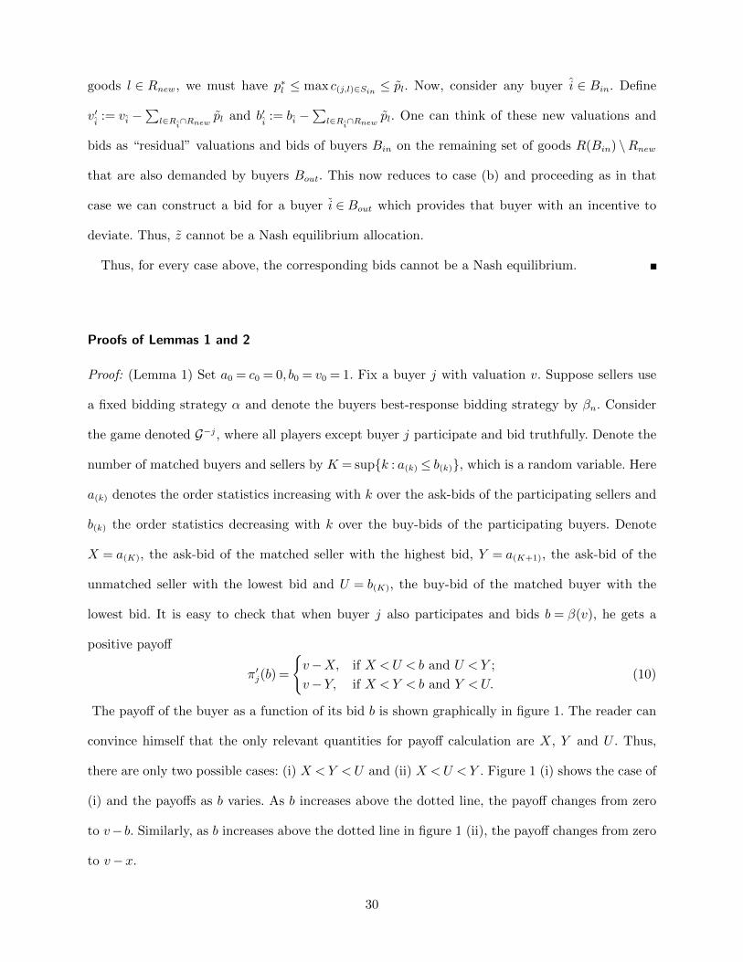
The payoff of the buyer as a function of its bid b is shown graphically in figure 1. The reader can

convince himself that the only relevant quantities for payoff calculation are X, Y and U . Thus,

there are only two possible cases: (i) X <Y <U and (ii) X <U <Y . Figure 1 (i) shows the case of

(i) and the payoffs as b varies. As b increases above the dotted line, the payoff changes from zero

to v− b. Similarly, as b increases above the dotted line in figure 1 (ii), the payoff changes from zero

to v−x.

30

X

Y

U

0b

b

b

b

0

v-y

v-y

X

Y

Ub

b

b

b

v-x

v-x

0

0

b+ b

b+ b

b

b

(i) (ii)

Figure 1 The payoff of the buyer as a function of its bid b for various cases.

The expected payoff denoted by π′j satisfies the differential equation

dπ′jdb

= P n(Ab,b)nf(b)(v− b) +

∫ b

0

P n(Bx,b)nf(x)(n− 1)g(b)(v−x)dx, (11)

where

P n(Ax,y) =n−1∑k=0

(n− 1

k

)F k(x)F n−1−k(x)

(n− 1

k

)Gk(y)Gn−1−k(y)

is the probability of the event that X = x and Y = y with x < y, among n− 1 sellers and n− 1

buyers. Similarly,

P n(Bx,y) =n−1∑k=1

(n− 1

k− 1

)F k−1(x)F n−k(x)

(n− 2

k− 1

)Gk−1(y)Gn−1−k(y)

is the probability of the event that X = x and Y = y with x < y, among n− 1 sellers and n− 2

buyers.

The boundary condition for the differential equation is π′j(0) = 0. The first term above arises

from the change in payoff when b is increased by ∆b and U > Y > b > X, and b + ∆b > Y as

shown in figure 1(i). Similarly, the second term is the change in payoff when Y > U > b >X and

b+ ∆b > U as shown in figure 1(ii). It is clear from (11) that for b ≤ v,dπ′jdb> 0. Given that the

sellers play strategy α, the best-response strategy of the buyers βn is such that b = βn(v) and

dπ′jdb

= 0. From this it is clear that b= βn(v)≥ v, ∀n≥ 2.

31

Proof: (Lemma 2) Set a0 = c0 = 0, b0 = v0 = 1. Fix a seller i with cost c. Consider the auction game,

denoted G−i, in which seller i does not participate and all participating buyers bid truthfully. As

before, denote the number of matched buyers and sellers by K = sup{k : a(k) ≤ b(k)}, U = b(K), the

bid of the lowest matched buyer, W = b(K+1), the bid of the highest unmatched buyer, X = a(K),

the bid of the highest matched seller, Y = a(K+1), the bid of the lowest unmatched seller, and

Z = a(K−1), the bid of the next highest matched seller.

a a-c

(i)

Z

X

W

x-ca

a

a

a

x-c

a-c

0

Z

X

Wz-ca

a

a

a

a-c

0

z-c

Z

X

Wa

a

a

0

a-c

z-c

(ii) (iii)

a

a a

Da

a

a a

Ea

a

a a

EaAa

Ba

CaCa

Figure 2 The payoff of the seller as a function of its bid a for various cases.

Consider the payoff of the i-th seller when he participates as well. His payoff when he bids

a= α(c) is given by

πi(a) =

x− c, if a<Z <X <W, or

Z < a<X <W ;

a− c, if Z <X <a<W, or

Z < a<W <X, or

Z <W <a<X, or

W <Z <a<X;

z− c, if a<Z <W <X, or

a<W <Z <X, or

W <a<Z <X.

(12)

The payoff of the seller as his bid a varies is shown graphically in figure 2. The reader can

convince himself that the only relevant quantities for payoff calculation are X, Z and W . Thus,

there are three cases: (i) Z <X <W , (ii) Z <W <X and (iii) W <Z <X.

32

The expected payoff denoted by πi satisfies the differential equation

dπi(a)

da= [P n(Aa) +P n(Ba) +P n(Ca)]

−[ng(a)P n(Da) + (n− 1)f(a)P n(Ea)](a− c), (13)

with the boundary condition πi(1) = 0 where Aa denotes the event that there are n− 1 sellers and

n buyers and X < a <W . As a is increased by ∆a, the payoff to the seller also increases by ∆a

since seller i is the price-determining seller. Similarly, Ba denotes the event that there are n− 1

sellers and n buyers and Z < a <W <X and seller i is the price-determining seller. In the same

way, Ca denotes the event that there are n− 1 sellers, n buyers and max(Z,W )<a<X and seller

i is the price-determining seller. Da denotes the event that there are n−1 sellers and n−1 buyers,

X <a (with the n-th buyer bidding a) and W ∈ [a,a+ ∆a] so that the seller i becomes unmatched

as it increases its bid. Similarly, Ea is the event that there are n−2 sellers, n buyers, W <a (with

the (n− 1)-th seller bidding a) and X ∈ [a,a+ ∆a]. And so as he increases his bid, he becomes

unmatched.

Figure 2 shows these events graphically. Events Aa, Ba and Ca correspond to various cases when

the change in the bid a from a to ∆a, causes a change in payoff of ∆a. Events Da and Ea correspond

to cases when the change in the bid a from a+ ∆a, causes a change in payoff of −(a− c).

The following can then be obtained:

P n(Aa) =n−1∑k=0

(n− 1

k

)F k(a)F n−1−k(a)

(n

k+ 1

)Gk+1(a)Gn−(k+1)(a)

P n(Ba) =n−1∑k=1

(n− 1

k− 1

)F k−1(a)F n−k(a)

(n

k+ 1

)Gk+1(a)Gn−(k+1)(a)

P n(Ca) =n−1∑k=1

(n− 1

k− 1

)F k−1(a)F n−k(a)

(n

k

)Gk(a)Gn−k(a)

P n(Da) =n−1∑k=0

(n− 1

k

)F k(a)F n−1−k(a)

(n− 1

k

)Gk(a)Gn−1−k(a)

P n(Ea) =n−1∑k=1

(n− 2

k− 1

)F k−1(a)F n−1−k(a)

(n

k

)Gk(a)Gn−k(a). (14)

33

Let a= αn(c) be the best-response strategy of the sellers. Then, dπida

= 0 at a= αn(c). For any

a< c, dπida> 0 from (13). Thus,

a= αn(c)≥ c, ∀n≥ 2. (15)

If a> c, setting (13) equal to zero and rearranging, we get

f(a) =[P n(Aa) +P n(Ba) +P n(Ca)]−ng(a)P n(Da)(a− c)

(n− 1)P n(Ea)(a− c)≥ 0,

from which we obtain

αn(c)− c ≤ [P n(Aa) +P n(Ba) +P n(Ca)]

ng(a)P n(Da)(16)

≤ 1

g(a)

∑n−1

k=0

(n−1k

)2 zk

(k+1)∑n−1

k=0

(n−1k

)2zk

G+

∑n−1

k=1

(n−1k

)2 zk

(n−k)∑n−1

k=0

(n−1k

)2zk

GF

F

+

1

g(a)

∑n−1

k=1

(n−1k

)2 kzk

(n−k)2∑n−1

k=0

(n−1k

)2zk

F

F

,where z = F (a)G(a)

F (a)G(a). Observe that the terms G(a), G(a)F (a) and F (a) in the numerator are

upper-bounded by one, and the term F (a) in the denominator is lower-bounded by F (c). It can

now be shown that each of the terms converges to zero for all z > 0 as n→ 0. Thus, (αn, β)→ (α, β).

Proof of Theorem 4

Proof: We first show the existence of (x∗, y∗) and (λ∗1, · · · , λ∗L), the dual variables corresponding

to the demand less than equal to supply constraints. We do this by casting the cLP above as an

optimal control problem and then appeal to Pontryagin’s maximum principle (?). Define

ζ(t) := Σmi=1x(t)δ(t)p(t)I(t∈Bi)−Σn

j=1y(t)σ(t)q(t)I(t∈ Sj), (17)

ξl(t) :=n∑j=1

y(t)σ(t)I(l ∈Lj, t∈ Sj)−m∑i=1

x(t)δ(t)I(l ∈Ri, t∈Bi), (18)

θ(t) := (ξ1(t), · · · , ξL(t), ζ(t))′, (19)

34

where θ is the state of the system, x and y are controls, and ζ(t) and ξ(t) describe the state

evolution as a function of the controls. The objective is to find the optimal control (x∗, y∗) which

maximizes ζ(1). Let

Σ(t) := {θ(t) : xl(0) = 0,∀l and x(t), y(t)∈ {0,1},∀t∈ [0,1]}. (20)

Observe that Σ(t) has cardinality at most 2L+1 in RL+1.∫ 1

0Σ(τ)dτ is the set of reachable states

under the set of all allowed control functions, namely, all measurable functions x and y such that

x(τ), y(τ)∈ {0,1}. Note that ζ(1) defines our total surplus; i.e., buyer surplus minus seller surplus,

and ξl(1) defines the excess supply for item l; i.e., total supply minus total demand for item l.

Define

Γ := {θ(1)∈RL+1 : θ(1)∈∫ 1

0

Σ(τ)dτ, ξl(1)≥ 0,∀l}, (21)

the set of final reachable states under all control functions such that state evolution happens

according to the equations above, and excess supply is non-negative.

Lemma 3. Γ is a compact, convex set.

Proof: By assumption, δ(t), p(t), σ(t), and q(t) are bounded. By Lyapunov’s theorem (Aumann

1965),∫ 1

0Σ(τ)dτ is a closed and convex set. Since x and y are bounded functions, the integral is

bounded as well. Thus, it is also compact. Moreover, ξl(1) is a hyperplane, and ξ(1) ≥ 0 defines

a closed subset of RL. Therefore, {θ(1) : θ(1) ∈∫ 1

0Σ(τ)dτ}

⋂{θ(1) : ξl(1) ≥ 0, l = 1, · · · ,L} is a

compact, convex set.

Now, our optimal control problem is: supθ(1)∈Γ ζ(1). But observe that one component of θ(1) is

ζ(1). Since Γ is compact and convex, the supremum is achieved and an optimal control (x∗, y∗)

exists in Γ. By the maximum principle (Varaiya 1971), there exist adjoint functions p∗0(t) and p∗l (t),

l= 1, · · · ,L such that p∗0(t) = 0, and p∗l (t) = 0, (i.e., p∗l (t) = λ∗l , a constant) for l= 0, · · · ,L.

Defining the Lagrangian over the objective function and the demand less than equal to supply

constraint

L(x, y;λ) = ζ(1) +L∑l=1

λlξl(1), (22)

35

we get from the saddle-point theorem (Varaiya 1971),

L(x, y;λ∗)≤L(x∗, y∗;λ∗)≤L(x∗, y∗;λ). (23)

We use this saddle point inequality to conclude the existence of a competitive equilibrium.

Lemma 4. If ((x∗, y∗), λ∗) is a saddle point satisfying the inequality (23) above, then the λ∗ are

competitive equilibrium prices. Moreover, pl ≤ λ∗l ≤ pl,∀l= 1, · · · ,L.

Proof: Let ((x∗, y∗), λ∗) be the saddle point satisfying the above inequality. Rewrite the Lagrangian

as

L(x, y;λ) =m∑i=1

∫Bi

δ(t)x(t)(p(t)−∑l∈Rt

λl)dt+n∑j=1

∫Sj

σ(τ)y(τ)(λl(τ)− q(τ))dτ

where l(τ) is the item offered by seller τ . Now, using the first saddle-point inequality, we get that

x∗(t) = I(p(t)> Σl∈Rtλ∗l ) and y∗(τ) = I(q(τ)< λ∗l(τ)), which implies that the Lagrange multipliers

are competitive equilibrium prices. To prove the second part, note that by definition, for a given τ ,

y(τ)> 0 implies that q(τ)≤ λ∗l for τ ∈ Sl, which implies the first inequality. Again from definition,

we get that y(τ) = 0 implies that q(τ)≥ λ∗l for τ ∈ Sl, which implies the second inequality.

To conclude the proof of the theorem, we observe that if q is continuous and non-decreasing in

each interval Sj of [0,1], then pl = pl for each l, which then equals λ∗l by Lemma 4.

References

C.D.Aliprantis and K.C.Border, Infinite Dimensional Analysis: A Hitchhiker’s Guide, Springer-Verlag,

1999.

K. Arrow, “The property rights doctrine and demand revelation under incomplete information”, in Eco-

nomics and Human Welfare, ed. M. Boskin, 1979.

K. J. Arrow and F. H. Hahn, General Competitive Analysis, Holden-Day, 1971.

C. d’Aspremont and L-A. Gerard-Varet, “Incentives and incomplete information”, J. of Public Eco-

nomics, 11:25-45, 1979.

R. J. Aumann, “Markets with a continuum of traders”, Economterica 32(1):39-50, 1964.

36

R. J. Aumann, “Integrals of set-valued functions”, J. Mathematical Analysis and Applications, 12:1-12,

1965.

L. M. Ausubel and P. Milgrom, “Ascending Auctions with Package Bidding”, Frontiers of Theoretical

Economics, 1(1):1-43, 2002.

M. Babaioff and W. Walsh, “Incentive-Compatible, Budget-Balanced, yet Highly Efficient Auctions for

Supply Chain Formation”, Decision Support Systems, 39(1):123-149, 2005.

S. Bikhchandani, S. de Vries, J. Schummer and R. Vohra, “Linear programming and Vickrey auc-

tions”, Mathematics of the Internet: E-Auctions and Markets. IMA Volumes in Mathematics and its

Applications, 75-116, 2001.

K. Chatterjee and W. Samuelson, “Bargaining under incomplete information”, Operations Research,

31:835-851, 1983.

L.Y. Chu and Z-J. Max Shen, “Truthful double auction mechanisms, Operations Research 56(1):102-120,

2008.

P. Dasgupta and E. Maskin, “Efficient Auctions”, Quaterly J. of Economics, 115(2):341-388, 2000.

D. Fudenberg, M. Mobius and A. Szeidl, “Existence of Equilibrium in Large Double Auctions”, Journal

of Economic Theory 133(1):550-567, 2007.

D. Fudenberg and J. Tirole, Game Theory, MIT Press, 1991.

D. Gale, Strategic Foundations of General Equilibrium, Cambridge University Press, 2000.

J. R. Green and J.-J. Laffont, “Characterization of satisfactory mechanisms for the revelation of pref-

erences for public goods”, Econometrica, 45:427-438, 1979

T. Gresik and M. Satterthwaite, “The rate at which market converges to efficiency as the number of

traders increases: An asymptotic result for optimal trading mechanism”, J. Economic Theory, 48:304-

332, 1989.

F. Gul and A. Postlewaite, “Asymptotic efficiency in large exchange economies with assymetric infor-

mation”, Econometrica, 60(6):1273-1292, 1992.

J. Harsanyi, “Games with incomplete information played by Bayesian players”, Parts I,II, and III, Man-

agement Science, 14:159-182, 320-334, 486-502, 1967-68.

37

L. Hurwicz, “On informationally decentralized systems”, In C. McGuire and R. Radner, eds., Decision and

Organization: A Volume in Honor of Jacob Marchak, North-Holland, 1975.

M. Jackson, “Incentive compatibility and competitive allocations”, Economics Lett., 40:299-302, 1992.

M. Jackson and A. Manelli, “Approximately competitive equilibria in large finite economies”, J. Eco-

nomic Theory 77(2):354-376, 1997.

M. Jackson and J. Swinkels, “Existence of Equilibrium in Single and Double Private Value Auctions

”,Econometrica 73(1):93-139, 2005.

R. Jain and P. Varaiya, “Combinatorial Bandwidth Exchange: Mechanism Design and Analysis”, Com-

munications in Information and Systems, 3(4):305-324, 2004.

R. Jain and J. Walrand, “An efficient Nash implementation mechanism for divisible resource allocation”,

Automatica, August 2010.

R. Johari and J. N. Tsitsiklis, “Efficiency loss in a network resource allocation game”, Mathematics of

Operations Research, 29(2):407-435, 2004.

C. Kaskiris, R. Jain, R. Rajagopal and P. Varaiya, “Combinatorial auction design for bandwidth

trading: An experimental study”, in Developments in Experimental Economics, Springer Lecture Notes

in Economics and Mathematical Systems, 2007.

E. Kazumori, “Towards a strategic theory of markets with incomplete information: Existence of Isotone

Equilibrium”, Working paper, 2003.

F. P. Kelly, A. K. Maullo and D. K. H. Tan, “Rate control in communication networks: shadow

prices, proportional fairness and stability”, J. of the Operational Research Soc., 49(1):237-252, 1998.

P. Klemperer, “Auction theory: A guide to the literature”, J. Economic Surveys, 13(3):227-286, 1999.

V. Krishna, Auction Theory, Academic Press, 2002.

V. Krishna and M. Perry, “Efficient Mechanism Design”, Working paper, 1998.

B. LeBrun, “Existence of equilibrium in first-price auctions”, Economic Theory, 7(3), 421-443, 1996.

J. K. MacKie-Mason and H. Varian, “Pricing congestible network resources”, IEEE J. Selected Areas

in Communication, 13(7):1141-1149, 1995.

A. Mas-Colell and X. Vives, “Implementation in economies with a continuum of agents”, Rev. Economic

Studies, 60(3):613-629, 1993.

38

A. Mas-Collel, M. Whinston and J. Green, Microeconomic Theory, Oxford University Press, 1995.

D. McAdams, “Monotone Equilibrium in Multi-unit Auctions”, Review of Economic Studies 73(4):1039-

1056, 2006.

P. Milgrom “Putting auction theory to work: The simultaneous ascending auction”, J. Political Economy,

108(2):245-272, 2000.

P.Milgrom and C.Shannon, “Monotone comparative statics”, Econometrica, 62(1):157-180, 1994.

R. B. Myerson and M. A. Satterthwaite, “Efficient mechanisms for bilateral trading”, J. Economic

Theory, 28:265-281, 1983.

D. Parkes, Iterative Combinatorial Auctions: Achieving Economic and Computational Efficiency, PhD

Thesis, University of Pennsylvania, 2001.

D. Parkes, J. Kalagnanam and M. Eso, “Achieving Budget-Balance with Vickrey-Based Payment

Schemes in Exchanges”, Proc. International Joint Conference on Artificial Intelligence, 2001.

M. Perry and P. Reny, “An Efficient Multi-Unit Ascending Auction”, Review of Economic Studies,

72(2):567-592, April 2005.

J. Quintero, “Combinatorial Electricity Auctions”, unpublished document, 2001.

D. Roberts and A. Postlewaite, “The incentives for price-taking behavior in large economies”, Econo-

metrica, 44(1):115-127, 1976.

A. Ronen, Solving Optimization Problems Among Selfish Agents, PhD Thesis, Hebrew University, 2000.

A. Rustichini, M. Satterthwaite and S. Williams, “Convergence to efficiency in a simple market with

incomplete information”, Econometrica, 62(5):1041-1063, 1994 .

T. Sandholm, “Algorithm for optimal winner determination in combinatorial auctions”, Artificial Intelli-

gence, 135:1-54, 2002.

M. Satterthwaite and S. Williams, “Bilateral trade with the sealed bid k-double auction: Existence

and efficiency”, J. Economic Theory, 48:107-133, 1989.

M. Satterthwaite and S. Williams, “The rate of convergence to efficiency in the buyer’s bid double

auction as the market becomes large”, Rev. Economic Studies, 56:477-498, 1989.

M. Satterthwaite and S. Williams, “The optimality of a simple market mechanism”, Econometrica

70(5):1841-1863, 2002.

39

W. Vickrey, “Counterspeculation, auctions, and sealed tenders”, J. Finance, 16:8-37, 1961.

A. Whinston, A. Gupta and D.O. Stahl, “An Economic Approach to Network Computing With Priority

Classes”, Journal of Organizational Computing and Electronic Commerce,” 6(1):71-95, 1996.

S. Williams, “Existence and convergence to equilibria in the buyer’s bid double auction”, Rev. Economic

Studies, 58:351-374, 1991.

P. P. Varaiya, Lecture Notes on Optimization, Nostrand-Holland, 1971.

S. de Vries and R. Vohra, “Combinatorial auctions: A survey”, Informs J. Computing, 15(3):284-309,

2003.

R. Wilson, “Incentive efficiency of double auctions”, Econometrica, 53(5):1101-1115, 1985.

S. Yang and B. Hajek, “VCG-Kelly mechanisms for allocation of divisible goods: Adapting VCG mecha-

nisms to one-dimensional signals, IEEE J. Selected Areas of Communications 25:1237-1243, 2007.

K. Yoon, “The modified Vickrey double auction”, J. Economic Theory, 101:572-584, 2001.

40