An Assessment of Transport Property Estimation Methods for ...orbit.dtu.dk/files/110304601/Nakai_et_al_abstract.pdf · International Journal of Thermophysics manuscript No. (will

General rights Copyright and moral rights for the publications made accessible in the public portal are retained by the authors and/or other copyright owners and it is a condition of accessing publications that users recognise and abide by the legal requirements associated with these rights.

• Users may download and print one copy of any publication from the public portal for the purpose of private study or research. • You may not further distribute the material or use it for any profit-making activity or commercial gain • You may freely distribute the URL identifying the publication in the public portal

If you believe that this document breaches copyright please contact us providing details, and we will remove access to the work immediately and investigate your claim.

Downloaded from orbit.dtu.dk on: Jun 05, 2018

An Assessment of Transport Property Estimation Methods for Ammonia–WaterMixtures and Their Influence on Heat Exchanger Size

Kærn, Martin Ryhl; Modi, Anish; Jensen, Jonas Kjær; Haglind, Fredrik

Published in:International Journal of Thermophysics

Link to article, DOI:10.1007/s10765-015-1857-8

Publication date:2015

Document VersionPeer reviewed version

Link back to DTU Orbit

Citation (APA):Kærn, M. R., Modi, A., Jensen, J. K., & Haglind, F. (2015). An Assessment of Transport Property EstimationMethods for Ammonia–Water Mixtures and Their Influence on Heat Exchanger Size. International Journal ofThermophysics, 36(7), 1468-1497. DOI: 10.1007/s10765-015-1857-8

http://dx.doi.org/10.1007/s10765-015-1857-8

http://orbit.dtu.dk/en/publications/an-assessment-of-transport-property-estimation-methods-for-ammoniawater-mixtures-and-their-influence-on-heat-exchanger-size(35dc4918-5380-48f0-b2b0-a351e965a661).html

International Journal of Thermophysics manuscript No.(will be inserted by the editor)

An Assessment of Transport Property Estimation Methods

for Ammonia-Water Mixtures and their Influence on Heat

Exchanger Size

M.R. Kærn · A. Modi · J.K. Jensen ·F. Haglind

Received: date / Accepted: date

Abstract Transport properties of fluids are indispensable for heat exchanger design.The methods for estimating the transport properties of ammonia-water mixtures arenot well established in the literature. The few existent methods are developed fromnone or limited, sometimes inconsistent experimental data sets, conducted for theliquid phase only. These data sets are usually confined to low concentrations andtemperatures, which are much less than those occurring in Kalina cycle boilers.

This paper presents a comparison of various methods used to estimate the vis-cosity and the thermal conductivity of ammonia-water mixtures. Firstly, the differentmethods are introduced and compared at various temperatures and pressures. Sec-ondly, their individual influence on the required heat exchanger size (surface area) isinvestigated. For this purpose, two case studies related to the use of the Kalina cy-cle are considered: a flue-gas-based heat recovery boiler for a combined cycle powerplant and a hot-oil-based boiler for a solar thermal power plant.

The different transport property methods resulted in larger differences at highpressures and temperatures, and a possible discontinuous first derivative, when usingthe interpolative methods in contrast to the corresponding state methods. Neverthe-less, all possible mixture transport property combinations used herein resulted in aheat exchanger size within 4.3 % difference for the flue-gas heat recovery boiler, andwithin 12.3 % difference for the oil-based boiler.

Keywords Ammonia-water · Heat transfer · Heat exchanger design · Kalina cycle ·Modeling · Transport properties · Zeotropic mixture

M.R. Kærn · A. Modi · J.K. Jensen · F. HaglindDepartment of Mechanical Engineering, Technical University of Denmark, Nils Koppels Allé Bygn. 403,DK-2800 Kgs. Lyngby, DenmarkTel.: +45 4525 4121Fax: +45 4593 5215E-mail: [email protected]

2 M.R. Kærn et al.

Nomenclature

RomanA area (m2)At total outer surface area (m2)cp specific heat capacity at constant pressure (J·kg−1·K−1)cv specific heat capacity at constant volume (J·kg−1·K−1)D outer diameter (m), dipole moment (debyes)d inner diameter (m)F interaction parameterG mass velocity or mass flux (kg·m−2·s−1)h heat transfer coefficient (W·m−2·K−1)k thermal conductivity (W·m−1·K−1), Boltzmann’s constantL length (m)m mass flow rate (kg·s−1)M molecular weight (g·mol−1)N number of parallel circuitsNu Nusselt numberp pressure (bar)Pr Prandtl numberQ heat flow rate (kW)Re Reynolds numberT temperature (K)U overall heat transfer coefficient (W·m−2·K−1)V molar volume (cm3·mol−1)x, x liquid mass and mole fractiony, y vapor mass and mole fractionZ bulk ammonia mass fraction

Greekα rotational coefficientρ molar density (mol·cm−3)ε energy-potential parameterη surface fin efficiencyκ polar association parameterµ dynamic viscosity (Pa·s)µ

m low-pressure gas viscosity (Pa·s)ω acentric fractorΩv viscosity collision integralσ molecular diameter (Å)

Subscriptsa ammoniac cold, criticalh hotm mixture

An Assessment of Transport Property Methods for Ammonia-Water Mixtures 3

r reducedw wall

Superscripts∗ correspondingˆ approximation¯ mean

AbbreviationsEV evaporatorEC economizerHRB heat recovery boilerOBB oil-based boilerSH superheater

1 Introduction

The zeotropic ammonia-water mixture has been used as a working fluid for decadesin various applications utilizing low-grade heat such as absorption refrigeration sys-tems, heat pumps, and power cycles. Reliable transport properties such as the viscos-ity and the thermal conductivity are always needed for the design of heat exchangersin such systems. The methods for estimating the transport properties of ammonia-water mixtures are not well established in the literature. The few existent methods aredeveloped from none or limited, sometimes inconsistent experimental data sets, con-ducted for the liquid phase only. Conde-Petit [1] proposed a set of methods tailoredfor ammonia-water mixtures in absorption refrigeration applications and comparedthese methods with the available experimental data in the literature. More recently,experimental data sets were obtained by Liu et al. [2] for the liquid dynamic viscosityand by Cuenca et al. [3] and Shamsetdinov et al. [4] for the liquid thermal conductiv-ity. Only the data set by Shamsetdinov et al. [4] included the full range of ammoniamass fractions and a large range of temperatures and pressures, whereas the formertwo data sets included small ranges of ammonia mass fractions (below 0.21), temper-atures and pressures. Even the standard property databases like the NIST standardizedreference database (REFPROP 9.12 [5]) do not allow for the transport property com-putation of polar mixtures such as ammonia-water. For these reasons, there is alwaysa need to verify the influence of the transport property estimation methods used for agiven heat exchanger design.

Both the plant efficiency and the cost (heat exchanger size) are important whencomparing an ammonia-water based system with other thermal energy systems. Oneof the main benefits of using the ammonia-water mixture as the working fluid is thepossibility of temperature matching between the heat source/sink and the workingfluid, thus decreasing thermal irreversibilities. In turn, the required heat transfer sur-face area might increase because of a smaller temperature difference between thefluids and influence negatively in the eventual economic advantage of a more effec-tive plant [6]. Additionally, the mixture boiling heat transfer coefficients are typicallyless than their pure counterparts [7, 8], thus leading to an even higher required heat

4 M.R. Kærn et al.

transfer surface area and cost. The boiling heat transfer degradation is mainly dueto the additional mass transfer resistance in the nucleate boiling region and changesin the transport properties in the convective boiling region [7]. A reliable estimationof the transport properties and thus the heat exchanger sizes are therefore imperativefor a full economic comparison of an ammonia-water based system with other sys-tems. When no validated transport property methods exists in the open literature, theinfluence of using different standard estimation methods must be evaluated.

To the authors’ knowledge, the only previous study in which the influence ofdifferent transport property methods are evaluated for ammonia-water systems, isthe study by Thorin [9]. The influence of two thermodynamic property correlations[6, 10] and two transport property correlations [6, 11] for the liquid and the vaporviscosity and thermal conductivity was assessed, and the differences in the heat ex-changer surface areas were as large as 24 % and 10 %, respectively, for individual heatexchangers in their Kalina cycle configuration. Furthermore, Thorin [9] argued thatseveral studies may be found in the literature in which the heat transfer processes ofammonia-water mixtures are involved, but they seldom report on the specific trans-port property methods used therein. Additionally, the method to evaluate the purecomponent transport properties, if needed by the mixture correlation, is typically notreported. The pure components might also be in different phases (liquid or vapor)compared with the mixture phase at the mixture temperature and pressure. Therefore,restriction should be imposed to ensure that the pure component estimations are inthe same phase as the mixture.

This paper compares various known transport property methods for the estima-tion of the liquid and the vapor viscosity and thermal conductivity of ammonia-watermixtures, and their individual influence on the required heat exchanger surface areaduring numerical design. The objective is to clarify whether the different transportproperty methods have a significant influence on the designed heat exchanger size.Two Kalina cycle case studies are considered for this purpose: a flue-gas-based heatrecovery boiler (HRB) for a combined cycle power plant and a hot-oil-based boiler(OBB) for a solar thermal power plant. Moreover, the two cases represent boilers witheither poor or good heat transfer characteristics on the secondary side. The boiler isusually the largest component in the Kalina cycle, taking up about half of the to-tal surface area [9] and destroying the most exergy [12]. In contrast to the work byThorin [9], several transport property estimation methods will be analyzed by simu-lating each possible combination individually, and a suitable two-phase heat transfercorrelation will be used instead of the fixed constant coefficient assumption by Thorin[9]. Finally, a discretized model is used that takes into account the local propertiesand heat transfer in the heat exchangers.

In total, 12 transport property methods are used during the numerical design forthe liquid and the vapor viscosity and thermal conductivity estimates. The actualestimates are graphically presented at various ammonia mass fractions, temperaturesand pressures, and compared to a few experimental data. All possible combinationsof transport property methods are simulated at different ammonia mass fractions andpressures in order to include several design conditions.

The outline of the paper is as follows: Sect. 2 introduces the transport property es-timation methods and correlations that have historically been proposed for ammonia-


water mixtures. Sect. 3 introduces the design models of the two case studies. Sect. 4presents the estimated heat exchanger sizes when using different transport propertymethods. Finally, the results are discussed in Sect. 5 and followed up by the conclu-sions in Sect. 6.

2 Transport Properties

Throughout this work, the NIST standardized reference database (REFPROP 9.12[5]) has been used to evaluate the thermodynamic properties. The latest so-called"Ammonia (Lemmon)" fluid file is used to select the ammonia-water mixture [13].The fluid file contains a refit of the ammonia equation of state that is compatiblewith the latest excess Helmholtz mixture model. The new ammonia-water mixtureformulation is more stable and faster [14] while giving outputs that are very close tothat of the earlier Tillner-Roth and Friend [10] formulation (REFPROP 9.0). For purecomponent transport properties, the same database is used while the critical mixtureproperties (temperature, pressure, and density) are evaluated using the experimentallyestablished formulations by Sassen et al. [15].

Many transport property estimation methods, for both pure components and mix-tures, have been gathered and described by Poling et al. [16]. The methods for mix-tures may be categorized to be either interpolative methods (e.g. the set of methodsproposed by Conde-Petit [1]) or corresponding state methods (e.g. the methods byChung et al. [17, 18]). Interpolative methods make use of the pure component trans-port properties evaluated at the same pressure and temperature as the mixture, whilethe corresponding state methods are based on pseudo-critical parameters and do notrequire the pure component transport properties. A includes all of the equations thatare used to estimate the transport properties used in this work, see Table 7 and 8, withthe exception of the mixing rules and the constant coefficients used in the methodsby Chung et al. [17, 18].

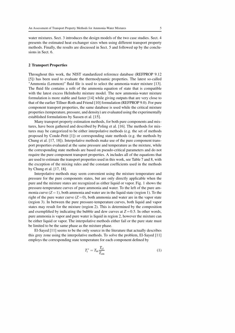
Interpolative methods may seem convenient using the mixture temperature andpressure for the pure components states, but are only directly applicable when thepure and the mixture states are recognized as either liquid or vapor. Fig. 1 shows thepressure-temperature curves of pure ammonia and water. To the left of the pure am-monia curve (Z=1), both ammonia and water are in the liquid state (region 1). To theright of the pure water curve (Z=0), both ammonia and water are in the vapor state(region 3). In between the pure pressure-temperature curves, both liquid and vaporstates may result for the mixture (region 2). This is determined by the compositionand exemplified by indicating the bubble and dew curves at Z=0.5. In other words,pure ammonia is vapor and pure water is liquid in region 2, however the mixture canbe either liquid or vapor. The interpolative methods either fail or the pure state mustbe limited to be the same phase as the mixture phase.

El-Sayed [11] seems to be the only source in the literature that actually describesthis grey zone using the interpolative methods. To solve the problem, El-Sayed [11]employs the corresponding state temperature for each component defined by

T ∗i = Tm

Tci

Tcm(1)

6 M.R. Kærn et al.

Mixture temperature, oC

Mix

ture

pre

ssure

, bar

Z=1

Z=0

Z=0.5

,bubble cu

rve

Z=0.5

,

dew c

urve

critical curve

region 1

region 2

region 3

0 50 100 150 200 250 300 350 400

0

50

100

150

200

250

Fig. 1 Pressure-temperature curves for pure ammonia (Z=1), pure water (Z=0) and a mixture at Z=0.5(bubble and dew curves). Region 1 (dark gray) is liquid for water, ammonia, and the mixture; Region 3(white) is vapor for ammonia, water, and the mixture; Region 2 (light gray) is vapor for ammonia, liquidfor water, but may be either vapor or liquid for mixture corresponding to composition

where Tm is the mixture temperature, Tci is the critical temperature of component i

and Tcm is the critical temperature of the mixture. The method limits the pure compo-nent state to be below its critical temperature. However, sometimes such a "pure" cor-responding state may lead to a non-existent pure state, e.g. at Tm=300 K and Z=0.1,the corresponding state temperature of ammonia becomes 300× (405.6/627.1)=194K,which is below the lower limit of ammonia in REFPROP. In other words, a generalinterpolation methodology does not exist. El-Sayed [11] used the corresponding statetemperature to evaluate the liquid viscosity and thermal conductivity; however forthe vapor viscosity and thermal conductivity, the mixture temperature and pressurewere used. The corresponding state temperature was also used by Teja and Rice [19]for the estimation of liquid viscosity. Similarly, Conde-Petit [1] proposed the samecorresponding temperature approach in his interpolation scheme, however again onlyfor liquid transport properties.

All other interpolative methods to be introduced herein use mixture temperatureand pressure for the pure component states. The fictive liquid ammonia and watervapor in region 2 are then evaluated as follows: For the pure liquid ammonia evalu-ation, we have limited the liquid state to be that of the saturated liquid at the sametemperature as the mixture. It is justified by the fact that pressure has little effecton liquid viscosity and thermal conductivity. If the mixture temperature is above thecritical temperature of ammonia, no liquid state of ammonia can be evaluated at thesame temperature as the mixture, thus we have limited the liquid ammonia state tobe that of the critical state. For the pure water vapor evaluation in region 2, we havelimited the vapor state to be that of saturated water vapor at the same temperature asthe mixture. For low pressure (dilute) gases this assumption holds true, but for highpressure (dense) gases the pressure/density effects become more important.

The strength of the corresponding state methods for mixtures (not to be confusedwith the pure corresponding state for interpolative methods) is that the pure com-ponent transport properties are not needed. In other words, such methods are purely


0 0.2 0.4 0.6 0.8 1

2

2.2

2.4

2.6

2.8

3

x 10−5

Dynam

ic v

iscosity, P

a ⋅

s

Ammonia mass fraction

0 0.2 0.4 0.6 0.8 1

2

2.2

2.4

2.6

2.8

3

x 10−5

Dynam

ic v

iscosity, P

a ⋅

s


250 300 350 400 450 5001.8

2

2.2

2.4

2.6

2.8

3x 10

−5

Dynam

ic v

iscosity, P

a ⋅

s

Temperature, oC

250 300 350 400 450 5001.8

2

2.2

2.4

2.6

2.8

3x 10

−5

Dynam

ic v

iscosity, P

a ⋅

s

Temperature, oC

Z=0.5, p=150 bar

a b

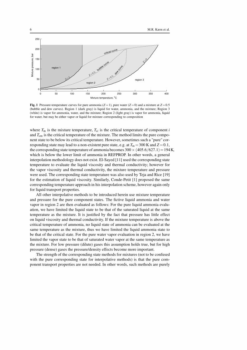
Fig. 2 Comparison of vapor viscosity methods. Curves (methods): Reichenberg [20]; Wilke[21]; Chung et al. [17, 18]; Chung et al. [17, 18] (composition averaged error). Symbols(conditions): T =325 C, p=50 bar; T =325 C, p=100 bar; T =425 C, p=100 bar; T =525C, p=100 bar;

predictive and thus generally applicable, however they tend to give higher errors thanthe interpolative methods [16]. If pure component transport properties are available,the estimation can be improved by using a composition-averaged error of the purecomponent predictions.

2.1 Vapor Viscosity

Fig. 2 shows four different vapor viscosity methods all of which are described inPoling et al. [16]. The first two listed methods (Reichenberg [20] and Wilke [21],Eqs. 16 and 15) are simplifications of the Chapman-Enskog kinetic theory extendedto mixtures and are interpolative. The third method is the corresponding state methodof Chung et al. [17, 18] (Eq. 17). It is also based on the Chapman-Enskog kinetictheory and is applicable for both high and low pressure gas mixtures. The fourthmethod corrects the corresponding state method of Chung et al. [17, 18] by using thecomposition-averaged error of the pure component predictions.

It should be noted that Fig. 2a shows results obtained only in region 3 of Fig. 1.In contrast, Fig. 2b shows results in regions 2 and 3.

Fig. 2a shows that the vapor viscosity depends more on the temperature than onthe pressure at these conditions. Changing the pressure from 50 to 100 bar at thesame temperature (325 C) does not have a significant effect on the pure componentviscosities and the interpolative methods, whereas the method of Chung et al. [17, 18]indicates a slightly larger significance of pressure. The method of Reichenberg [20]

8 M.R. Kærn et al.

is more complex than that of Wilke [21]. It suggests a parabolic trend, whereas Wilke[21] is almost linear with respect to composition. The latter method tends to be linear,because the interaction parameters (F12 and F21) are close to unity for ammonia-watermixtures, as the viscosities and molecular weights are similar. The correspondingstate method of Chung et al. [17, 18] results in a small error at the pure componentstates compared to the values suggested by REFPROP. The small error is consideredto be reasonable for a fully predictive method. When improving that method by thecomposition-averaged error of the pure components, it suggests nearly the same lineartrend as the method of Wilke [21]. The method of Wilke [21] has also been shown toperform well for other polar-polar compounds [16] which justifies its usage to someextent. The same method has been proposed by El-Sayed [11] and Conde-Petit [1]specific to ammonia-water mixtures.

Fig. 2b shows the problem of a nonexistent pure water vapor in region 2. Asalready mentioned, we limited the water vapor to be that of the saturated vapor at themixture temperature. For this reason, the methods that use the pure component vaporviscosities result in a C1 discontinuity (discontinuous first derivative) when crossingfrom region 2 to 3, i.e. at the saturation temperature of water (342 C at 150 bar). Thediscontinuity is not present in the corresponding state method of Chung et al. [17, 18]and highlights the strength of this fully predictive method. However, the discontinuityis small and vanishes at lower pressures.

2.2 Liquid Viscosity

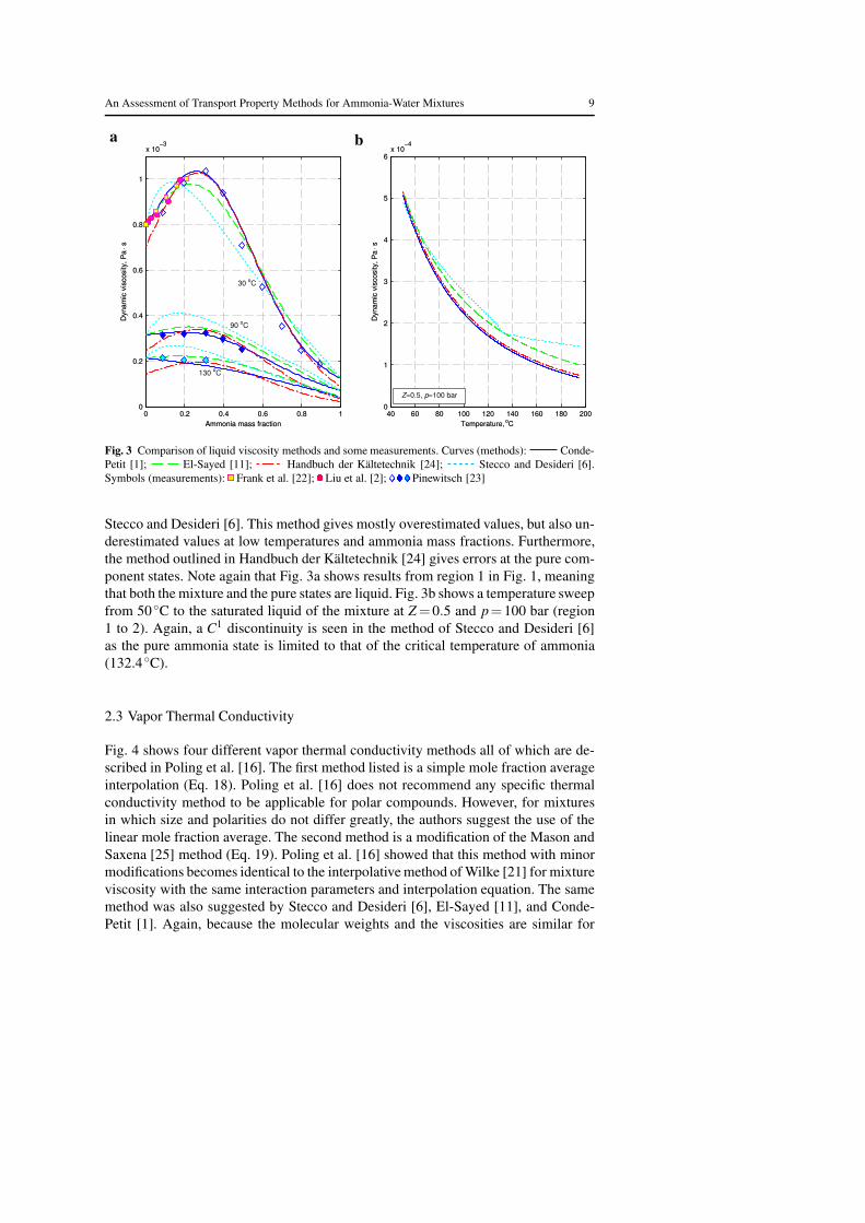
Regarding the estimation of both pure and mixture liquid viscosity, there is no theo-retical basis, and experimental data are particularly desirable. Fig. 3 illustrates fourdifferent liquid viscosity methods and their comparison to experimental data by Franket al. [22], Liu et al. [2] and Pinewitsch [23]. The first two listed (Conde-Petit [1] andEl-Sayed [11], Eqs. 7 and 8) have already been mentioned and are interpolative meth-ods using the “pure” corresponding state temperature approach. Note that the methodof El-Sayed [11] is misprinted in the original work, as pointed out by Thorin [9].The third method, proposed in Handbuch der Kältetechnik [24] (Eq. 9), was explic-itly developed for ammonia-water and based on a curve fit of experimental data. Ituses mixture temperature and composition directly, thus the pure component viscosi-ties are not required. The fourth method is a modified version of the Teja and Rice[19] method as used by Stecco and Desideri [6] (Eq. 10). The authors modified themethod by using the actual mixture temperature in the evaluation of the pure com-ponent viscosities instead of the pure corresponding state temperature. Additionally,the interaction parameter ψ was set to 8, which has also been suggested by El-Sayed[11]. All these methods take advantage of the liquid viscosity being nearly indepen-dent of pressure; thus when the pure component viscosities are needed, the saturatedliquid viscosity is used. All these methods are experimentally established, howeverthe method by Conde-Petit [1] has been established most recently and was developedusing the most number of experimental data points.

Fig. 3a shows that the methods correspond reasonably well to the experimen-tal data at various ammonia mass fractions and temperatures, except the method by


0 0.2 0.4 0.6 0.8 10

0.2

0.4

0.6

0.8

1

x 10−3

Dynam

ic v

iscosity, P

a ⋅

s


0 0.2 0.4 0.6 0.8 10

0.2

0.4

0.6

0.8

1

x 10−3

Dynam

ic v

iscosity, P

a ⋅

s


130 oC

90 oC

30 oC

40 60 80 100 120 140 160 180 2000

1

2

3

4

5

6x 10

−4

Dynam

ic v

iscosity, P

a ⋅

s

Temperature, oC

40 60 80 100 120 140 160 180 2000

1

2

3

4

5

6x 10

−4

Dynam

ic v

iscosity, P

a ⋅

s

Temperature, oC

Z=0.5, p=100 bar

a b

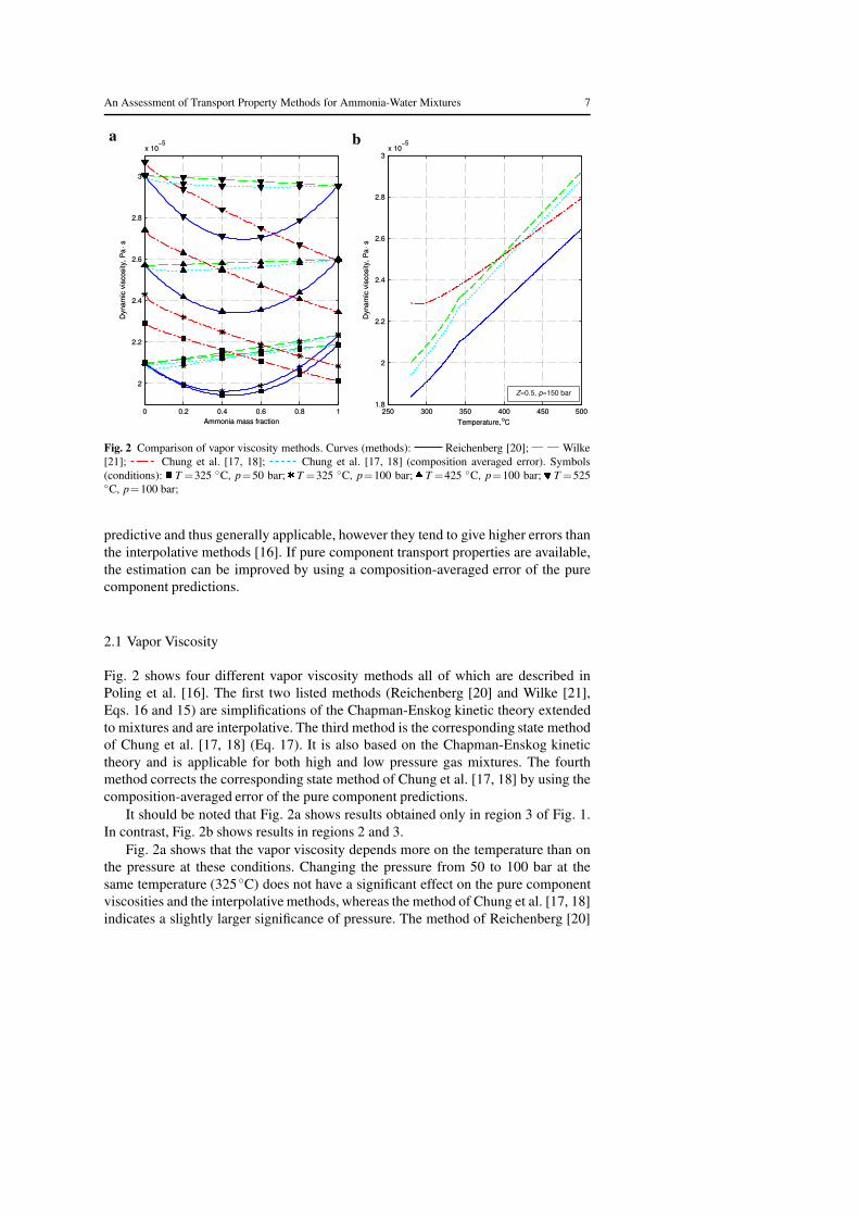
Fig. 3 Comparison of liquid viscosity methods and some measurements. Curves (methods): Conde-Petit [1]; El-Sayed [11]; Handbuch der Kältetechnik [24]; Stecco and Desideri [6].Symbols (measurements): Frank et al. [22]; Liu et al. [2]; Pinewitsch [23]

Stecco and Desideri [6]. This method gives mostly overestimated values, but also un-derestimated values at low temperatures and ammonia mass fractions. Furthermore,the method outlined in Handbuch der Kältetechnik [24] gives errors at the pure com-ponent states. Note again that Fig. 3a shows results from region 1 in Fig. 1, meaningthat both the mixture and the pure states are liquid. Fig. 3b shows a temperature sweepfrom 50 C to the saturated liquid of the mixture at Z =0.5 and p=100 bar (region1 to 2). Again, a C1 discontinuity is seen in the method of Stecco and Desideri [6]as the pure ammonia state is limited to that of the critical temperature of ammonia(132.4 C).

2.3 Vapor Thermal Conductivity

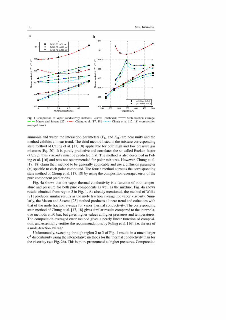
Fig. 4 shows four different vapor thermal conductivity methods all of which are de-scribed in Poling et al. [16]. The first method listed is a simple mole fraction averageinterpolation (Eq. 18). Poling et al. [16] does not recommend any specific thermalconductivity method to be applicable for polar compounds. However, for mixturesin which size and polarities do not differ greatly, the authors suggest the use of thelinear mole fraction average. The second method is a modification of the Mason andSaxena [25] method (Eq. 19). Poling et al. [16] showed that this method with minormodifications becomes identical to the interpolative method of Wilke [21] for mixtureviscosity with the same interaction parameters and interpolation equation. The samemethod was also suggested by Stecco and Desideri [6], El-Sayed [11], and Conde-Petit [1]. Again, because the molecular weights and the viscosities are similar for

10 M.R. Kærn et al.

0 0.2 0.4 0.6 0.8 10.05

0.06

0.07

0.08

0.09

0.1


Therm

al conductivity, W

⋅ m

−1⋅ K

−1

T=325

oC, p=50 bar

T=325 oC, p=100 bar

T=475 oC, p=100 bar

0 0.2 0.4 0.6 0.8 10.05

0.06

0.07

0.08

0.09

0.1


Therm

al conductivity, W

⋅ m

−1⋅ K

−1

200 250 300 350 400 450 5000.04

0.05

0.06

0.07

0.08

0.09

0.1

0.11

Temperature, oC

Therm

al conductivity, W

⋅ m

−1⋅ K

−1

p=50 bar, Z=0.5

p=150 bar, Z=0.5

200 250 300 350 400 450 5000.04

0.05

0.06

0.07

0.08

0.09

0.1

0.11

Temperature, oC

Therm

al conductivity, W

⋅ m

−1⋅ K

−1

a b

Fig. 4 Comparison of vapor conductivity methods. Curves (methods): Mole-fraction average;Mason and Saxena [25]; Chung et al. [17, 18]; Chung et al. [17, 18] (composition

averaged error)

ammonia and water, the interaction parameters (F12 and F21) are near unity and themethod exhibits a linear trend. The third method listed is the mixture correspondingstate method of Chung et al. [17, 18] applicable for both high and low pressure gasmixtures (Eq. 20). It is purely predictive and correlates the so-called Eucken-factor(k/µcv), thus viscosity must be predicted first. The method is also described in Pol-ing et al. [16] and was not recommended for polar mixtures. However, Chung et al.[17, 18] claim their method to be generally applicable and use a diffusion parameter(κ) specific to each polar compound. The fourth method corrects the correspondingstate method of Chung et al. [17, 18] by using the composition-averaged error of thepure component predictions.

Fig. 4a shows that the vapor thermal conductivity is a function of both temper-ature and pressure for both pure components as well as the mixture. Fig. 4a showsresults obtained from region 3 in Fig. 1. As already mentioned, the method of Wilke[21] produces similar results as the mole fraction average for vapor viscosity. Simi-larly, the Mason and Saxena [25] method produces a linear trend and coincides withthat of the mole fraction average for vapor thermal conductivity. The correspondingstate method of Chung et al. [17, 18] gives similar results compared to the interpola-tive methods at 50 bar, but gives higher values at higher pressures and temperatures.The composition-averaged error method gives a nearly linear function of composi-tion, and essentially verifies the recommendations by Poling et al. [16], i.e. the use ofa mole-fraction average.

Unfortunately, sweeping through region 2 to 3 of Fig. 1 results in a much largerC1 discontinuity using the interpolative methods for the thermal conductivity than forthe viscosity (see Fig. 2b). This is more pronounced at higher pressures. Compared to


0 0.2 0.4 0.6 0.8 10.3

0.35

0.4

0.45

0.5

0.55

0.6

0.65

0.7

Therm

al conductivity, W

⋅ m

−1⋅ K

−1


0 0.2 0.4 0.6 0.8 10.3

0.35

0.4

0.45

0.5

0.55

0.6

0.65

0.7

Therm

al conductivity, W

⋅ m

−1⋅ K

−1


T=30 oC

0 0.2 0.4 0.6 0.8 10.3

0.35

0.4

0.45

0.5

0.55

0.6

0.65

0.7

Therm

al conductivity, W

⋅ m

−1⋅ K

−1


0 0.2 0.4 0.6 0.8 10.3

0.35

0.4

0.45

0.5

0.55

0.6

0.65

0.7

Therm

al conductivity, W

⋅ m

−1⋅ K

−1


T=80 oC

0 0.2 0.4 0.6 0.8 1

0.2

0.3

0.4

0.5

0.6

0.7

Therm

al conductivity, W

⋅ m

−1⋅ K

−1


0 0.2 0.4 0.6 0.8 1

0.2

0.3

0.4

0.5

0.6

0.7

Therm

al conductivity, W

⋅ m

−1⋅ K

−1


T=130 oC

50 100 150 200 250

0.2

0.3

0.4

0.5

0.6

0.7

Therm

al conductivity, W

⋅ m

−1⋅ K

−1

Temperature, oC

50 100 150 200 250

0.2

0.3

0.4

0.5

0.6

0.7

Therm

al conductivity, W

⋅ m

−1⋅ K

−1

Temperature, oC

Z=0.5, p=100 bar

a b

c d

Fig. 5 Comparison of liquid thermal conductivity methods and some measurements. Curves (methods):Conde-Petit [1]; El-Sayed [11]; Filippov [27]; Jamieson et al. [28]. Symbols

(measurements): Cuenca et al. [3]; Shamsetdinov et al. [4]; Baranov et al. [26]

the corresponding state method of Chung et al. [17, 18], it is likely to be a nonphysicaldiscontinuity.

2.4 Liquid Thermal Conductivity

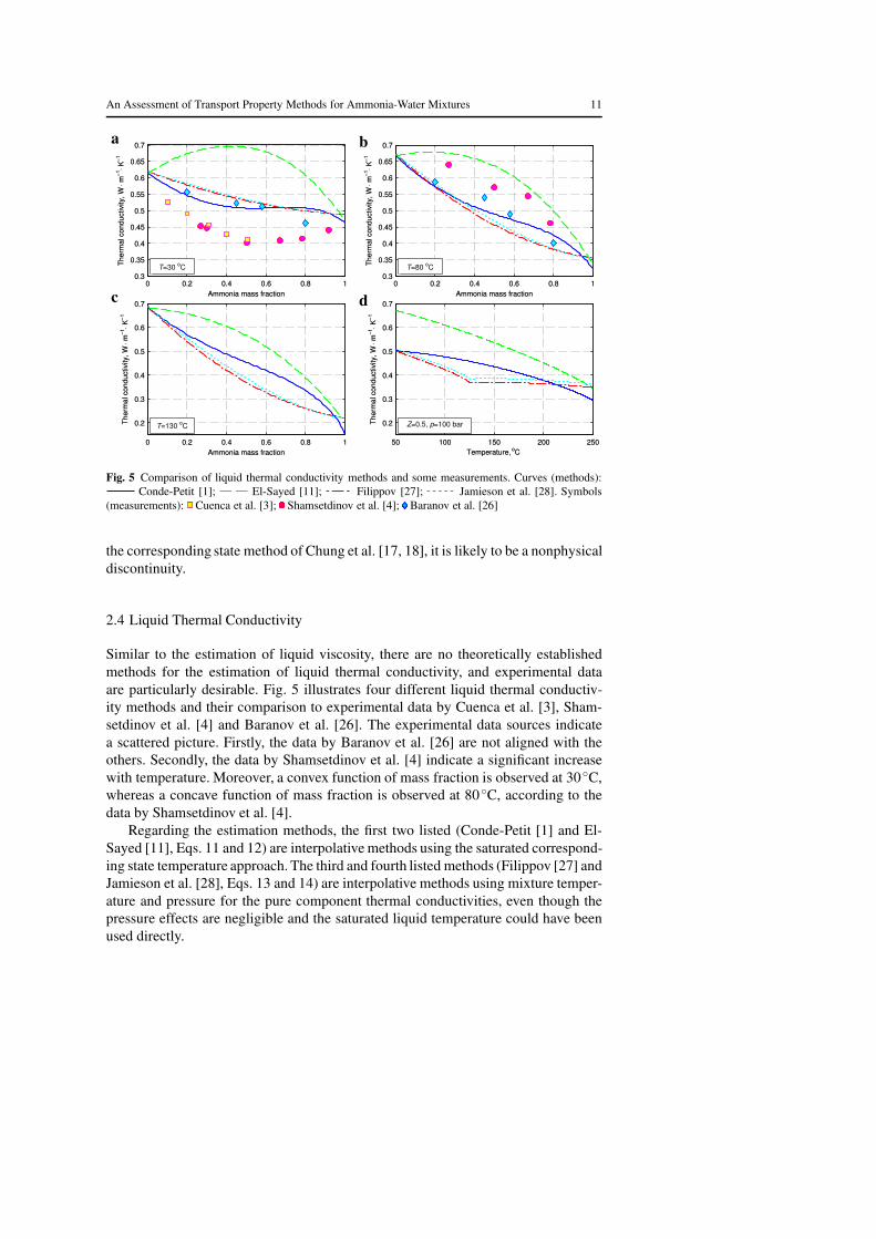
Similar to the estimation of liquid viscosity, there are no theoretically establishedmethods for the estimation of liquid thermal conductivity, and experimental dataare particularly desirable. Fig. 5 illustrates four different liquid thermal conductiv-ity methods and their comparison to experimental data by Cuenca et al. [3], Sham-setdinov et al. [4] and Baranov et al. [26]. The experimental data sources indicatea scattered picture. Firstly, the data by Baranov et al. [26] are not aligned with theothers. Secondly, the data by Shamsetdinov et al. [4] indicate a significant increasewith temperature. Moreover, a convex function of mass fraction is observed at 30 C,whereas a concave function of mass fraction is observed at 80 C, according to thedata by Shamsetdinov et al. [4].

Regarding the estimation methods, the first two listed (Conde-Petit [1] and El-Sayed [11], Eqs. 11 and 12) are interpolative methods using the saturated correspond-ing state temperature approach. The third and fourth listed methods (Filippov [27] andJamieson et al. [28], Eqs. 13 and 14) are interpolative methods using mixture temper-ature and pressure for the pure component thermal conductivities, even though thepressure effects are negligible and the saturated liquid temperature could have beenused directly.


Refering to Figs. 5a, 5b and 5c, the thermal conductivity of water exhibits a weakdependence on temperature, while the thermal conductivity of ammonia decreaseswith temperature. In fact water has a maximum in liquid thermal conductivity closeto 130-135 C, before decreasing at higher temperatures. Note that water at thesetemperatures and pressures is much subcooled. The figures show that the methodof El-Sayed [11] results in the concave function, the methods of Filippov [27] andJamieson et al. [28] result in the convex function, whereas the method of Conde-Petit[1] results in an S-shape function. It is difficult to judge which method performs thebest. At 80 C, it may be argued that the method of El-Sayed [11] performs the best,however at 30 C the method overestimates significantly (around 75% at Z = 0.5compared to Cuenca et al. [3] and Shamsetdinov et al. [4]). Overall, the method byConde-Petit [1] seems to perform the best and result in values close to the methods byFilippov [27] and Jamieson et al. [28]. Poling et al. [16] have shown that especiallythe method of Filippov [27] gave good results for some aqueous polar mixtures otherthan ammonia-water. However, it is only the method of Conde-Petit [1] that has beenexperimentally established even though these measurements also had remarkable in-consistencies [1].

Fig. 5d shows the transition from region 1 to 2 of Fig. 1 at p=100 bar and Z=0.5.Again, the limitation of the pure ammonia state to be liquid at its critical temperatureshows a C1 discontinuity in the methods of Filippov [27] and Jamieson et al. [28]. Incontrast, the corresponding state temperature approach by El-Sayed [11] and Conde-Petit [1] is smooth.

3 Model Development

This section presents the models of the HRB and the OBB, and explains the imple-mentation briefly. Then the HRB model is verified with earlier model results, andthe numerical convergence is duly analyzed for both models. The models are imple-mented in Dymola 2014 [29] using the Modelica language. All transport propertymethods used herein are freely available in the Modelica-REFPROP interface [30].

3.1 HRB Model

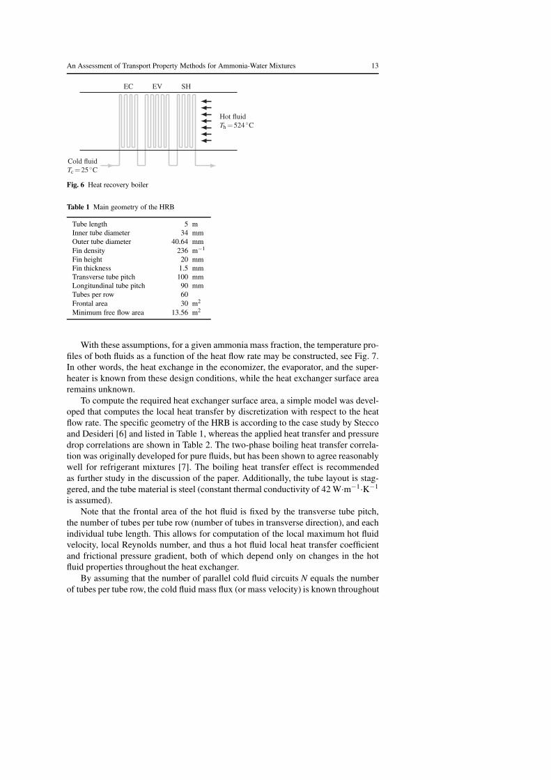
A sketch of the HRB is shown in Fig. 6. The HRB is recognized as a once-throughboiler having the cold fluid flowing inside a vertical tube bundle with external circularfins and the hot fluid flowing in a counter-cross flow arrangement. The hot fluid issimplified to be the product of a stoichiometric burning of methane and air (21 %O2, 79 % N2). The properties of the flue-gas are evaluated using the Modelica.Medialibrary, i.e. an ideal gas mixture. The inlet gas temperature and mass flow rate are524 C and 100 kg·s−1, respectively. The cold medium is the ammonia-water mixturewith an ammonia mass fraction, inlet temperature, and pressure of 0.7, 25 C and 40bar, respectively. The pinch point temperature difference is 15 K, and the approachtemperature difference (hot fluid inlet, cold fluid outlet) is 20 K. The ammonia massfraction and pressure are varied from 0.5 to 0.9 and from 40 to 100 bar, respectively,which are typical inlet conditions of the boiler in Kalina cycles [12, 31, 32].


Cold fluid

Tc=25C

Hot fluid

Th=524C

EC EV SH

Fig. 6 Heat recovery boiler

Table 1 Main geometry of the HRB

Tube length 5 mInner tube diameter 34 mmOuter tube diameter 40.64 mmFin density 236 m−1

Fin height 20 mmFin thickness 1.5 mmTransverse tube pitch 100 mmLongitundinal tube pitch 90 mmTubes per row 60Frontal area 30 m2

Minimum free flow area 13.56 m2

With these assumptions, for a given ammonia mass fraction, the temperature pro-files of both fluids as a function of the heat flow rate may be constructed, see Fig. 7.In other words, the heat exchange in the economizer, the evaporator, and the super-heater is known from these design conditions, while the heat exchanger surface arearemains unknown.

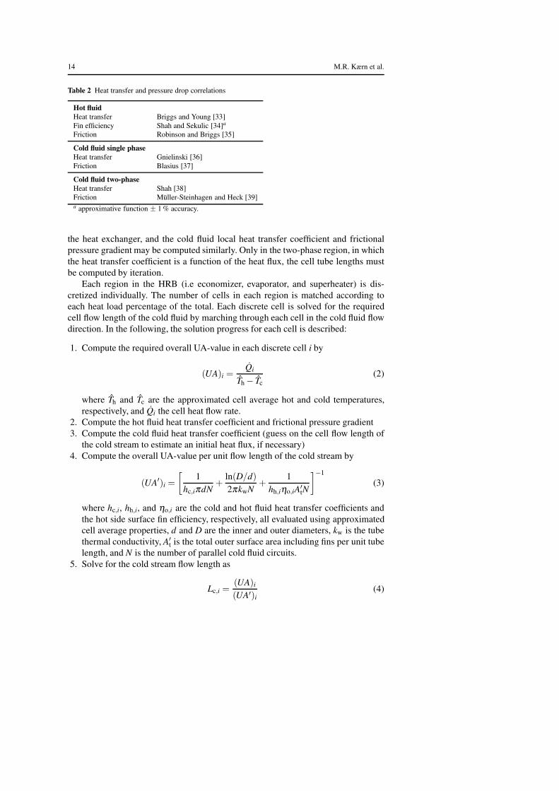
To compute the required heat exchanger surface area, a simple model was devel-oped that computes the local heat transfer by discretization with respect to the heatflow rate. The specific geometry of the HRB is according to the case study by Steccoand Desideri [6] and listed in Table 1, whereas the applied heat transfer and pressuredrop correlations are shown in Table 2. The two-phase boiling heat transfer correla-tion was originally developed for pure fluids, but has been shown to agree reasonablywell for refrigerant mixtures [7]. The boiling heat transfer effect is recommendedas further study in the discussion of the paper. Additionally, the tube layout is stag-gered, and the tube material is steel (constant thermal conductivity of 42 W·m−1·K−1

is assumed).Note that the frontal area of the hot fluid is fixed by the transverse tube pitch,

the number of tubes per tube row (number of tubes in transverse direction), and eachindividual tube length. This allows for computation of the local maximum hot fluidvelocity, local Reynolds number, and thus a hot fluid local heat transfer coefficientand frictional pressure gradient, both of which depend only on changes in the hotfluid properties throughout the heat exchanger.

By assuming that the number of parallel cold fluid circuits N equals the numberof tubes per tube row, the cold fluid mass flux (or mass velocity) is known throughout


Table 2 Heat transfer and pressure drop correlations

Hot fluid

Heat transfer Briggs and Young [33]Fin efficiency Shah and Sekulic [34]a

Friction Robinson and Briggs [35]

Cold fluid single phase

Heat transfer Gnielinski [36]Friction Blasius [37]

Cold fluid two-phase

Heat transfer Shah [38]Friction Müller-Steinhagen and Heck [39]a approximative function ± 1 % accuracy.

the heat exchanger, and the cold fluid local heat transfer coefficient and frictionalpressure gradient may be computed similarly. Only in the two-phase region, in whichthe heat transfer coefficient is a function of the heat flux, the cell tube lengths mustbe computed by iteration.

Each region in the HRB (i.e economizer, evaporator, and superheater) is dis-cretized individually. The number of cells in each region is matched according toeach heat load percentage of the total. Each discrete cell is solved for the requiredcell flow length of the cold fluid by marching through each cell in the cold fluid flowdirection. In the following, the solution progress for each cell is described:

1. Compute the required overall UA-value in each discrete cell i by

(UA)i =Qi

Th − Tc(2)

where Th and Tc are the approximated cell average hot and cold temperatures,respectively, and Qi the cell heat flow rate.

2. Compute the hot fluid heat transfer coefficient and frictional pressure gradient3. Compute the cold fluid heat transfer coefficient (guess on the cell flow length of

the cold stream to estimate an initial heat flux, if necessary)4. Compute the overall UA-value per unit flow length of the cold stream by

(UA′)i =

[

1hc,iπdN

+ln(D/d)

2πkwN+

1hh,iηo,iA

′tN

]−1

(3)

where hc,i, hh,i, and ηo,i are the cold and hot fluid heat transfer coefficients andthe hot side surface fin efficiency, respectively, all evaluated using approximatedcell average properties, d and D are the inner and outer diameters, kw is the tubethermal conductivity, A′

t is the total outer surface area including fins per unit tubelength, and N is the number of parallel cold fluid circuits.

5. Solve for the cold stream flow length as

Lc,i =(UA)i

(UA′)i

(4)


6. If the cold fluid heat transfer coefficient is a function of heat flux, repeat steps 3to 5 using the updated cold stream flow length until convergence. The total areais finally obtained by

At =n

∑i=1

A′tNLc,i (5)

7. Compute auxiliaries such as the number of tube rows, the cold fluid pressure drop,and the hot fluid pressure drop.

3.2 HRB Model Verification

The model is verified with numerical results obtained from Stecco and Desideri [6]at 0.7 ammonia mass fraction while using the same transport property methods. Noexperimental results have been found that are suitable for a HRB validation. Nev-ertheless, the model agrees well with the obtained numerical results as depicted inTable 3 for several important parameters. The total heat transfer surface area is pre-dicted within 6 %. The heat transfer coefficients match well for both the cold and hotfluids and show less than 4 % deviation, except that of the cold fluid in the superheaterwhich is over-predicted by 261 %. The cold fluid pressure drop is also over predictedin the superheater by 130 %. The results by Stecco and Desideri [6] indicate that thecircuitry (or geometry) must have been altered entering the superheater, such that thecold fluid mass flux decreases. Otherwise, the pressure drop cannot be lower than inthe evaporator for approximately the same heat exchanger size. In the current model,the cold fluid inlet and outlet velocities were 0.48 and 33.05 m·s−1, respectively. Thelatter, which is close to typical upper limits, could have been reduced by simply split-ting the cold streams, e.g. into twice as many parallel circuits, but it was not chosenbecause the pressure drop is of secondary interest in this work. Nevertheless, the totalhot fluid pressure drop matches well, and the deviation is within 10 % error.

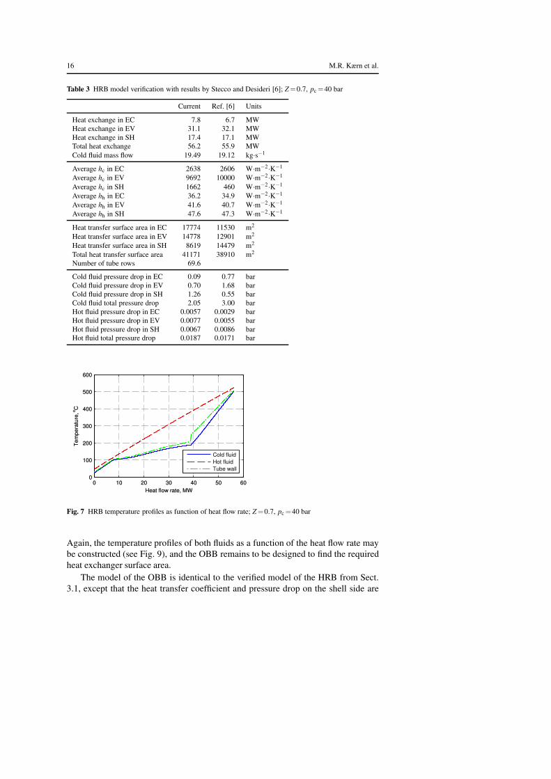
Fig. 7 shows the computed temperature profiles of the cold fluid, the hot fluid, andthe tube wall externally. It indicates that for this HRB, the hot fluid gas-side controlsthe heat transfer process, since the wall temperature is close to that of the cold fluid.In other words, the heat transfer resistance is highest on the gas-side. Hence, theeffects of different transport property methods used for the cold fluid ammonia-watermixture may have less importance for the HRB. This will be discussed in more detailin Sect. 4.

3.3 OBB Model

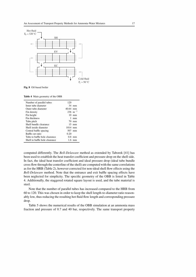
A sketch of the OBB is shown in Fig. 8. The OBB is recognized as several shell andtube heat exchangers having 1 shell pass for the hot fluid and 1 tube pass for the coldfluid. The tubes have circular fins and no tubes are placed in the window section.These options serve to enhance the heat transfer on the oil side while maintaininga low pressure drop. The hot fluid is Therminol 66, and the properties are obtainedfrom Solutia Inc. [40]. The conditions are almost the same as for the HRB, except thatthe cold fluid and the hot fluid inlet temperatures are 50 C and 320 C, respectively.


Table 3 HRB model verification with results by Stecco and Desideri [6]; Z=0.7, pc =40 bar

Current Ref. [6] Units

Heat exchange in EC 7.8 6.7 MWHeat exchange in EV 31.1 32.1 MWHeat exchange in SH 17.4 17.1 MWTotal heat exchange 56.2 55.9 MWCold fluid mass flow 19.49 19.12 kg·s−1

Average hc in EC 2638 2606 W·m−2·K−1

Average hc in EV 9692 10000 W·m−2·K−1

Average hc in SH 1662 460 W·m−2·K−1

Average hh in EC 36.2 34.9 W·m−2·K−1

Average hh in EV 41.6 40.7 W·m−2·K−1

Average hh in SH 47.6 47.3 W·m−2·K−1

Heat transfer surface area in EC 17774 11530 m2

Heat transfer surface area in EV 14778 12901 m2

Heat transfer surface area in SH 8619 14479 m2

Total heat transfer surface area 41171 38910 m2

Number of tube rows 69.6

Cold fluid pressure drop in EC 0.09 0.77 barCold fluid pressure drop in EV 0.70 1.68 barCold fluid pressure drop in SH 1.26 0.55 barCold fluid total pressure drop 2.05 3.00 barHot fluid pressure drop in EC 0.0057 0.0029 barHot fluid pressure drop in EV 0.0077 0.0055 barHot fluid pressure drop in SH 0.0067 0.0086 barHot fluid total pressure drop 0.0187 0.0171 bar

0 10 20 30 40 50 600

100

200

300

400

500

600

Heat flow rate, MW

Te

mp

era

ture

, oC

Cold fluid

Hot fluid

Tube wall

0 10 20 30 40 50 600

100

200

300

400

500

600

Heat flow rate, MW

Te

mp

era

ture

, oC

Fig. 7 HRB temperature profiles as function of heat flow rate; Z=0.7, pc =40 bar

Again, the temperature profiles of both fluids as a function of the heat flow rate maybe constructed (see Fig. 9), and the OBB remains to be designed to find the requiredheat exchanger surface area.

The model of the OBB is identical to the verified model of the HRB from Sect.3.1, except that the heat transfer coefficient and pressure drop on the shell side are


EC

EV

SH

Cold fluid

Tc =50C

Hot fluid

Th =320C

Fig. 8 Oil-based boiler

Table 4 Main geometry of the OBB

Number of parallel tubes 120Inner tube diameter 34 mmOuter tube diameter 40.64 mmFin density 236 m−1

Fin height 10 mmFin thickness 1 mmTube pitch 70 mmShell bundle clearance 15 mmShell inside diameter 1014 mmCentral baffle spacing 507 mmBaffle cut ratio 0.20Tube to baffle hole clearance 0.8 mmShell to baffle hole clearance 1.6 mm

computed differently. The Bell-Delaware method as extended by Taborek [41] hasbeen used to establish the heat transfer coefficient and pressure drop on the shell side.In fact, the ideal heat transfer coefficient and ideal pressure drop (ideal tube bundlecross flow through the centerline of the shell) are computed with the same correlationsas for the HRB (Table 2), however corrected for non-ideal shell flow effects using theBell-Delaware method. Note that the entrance and exit baffle spacing effects havebeen neglected for simplicity. The specific geometry of the OBB is listed in Table4. Additionally, the staggered rotated square layout is used, and the tube material issteel.

Note that the number of parallel tubes has increased compared to the HRB from60 to 120. This was chosen in order to keep the shell length-to-diameter ratio reason-ably low, thus reducing the resulting hot fluid flow length and corresponding pressuredrop.

Table 5 shows the numerical results of the OBB simulation at an ammonia massfraction and pressure of 0.7 and 40 bar, respectively. The same transport property


methods as used by Stecco and Desideri [6] are used to ensure a direct comparisonwith the HRB results from the previous section.

Table 5 OBB model results; Z=0.7, pc =40 bar

Heat exchange in EC 6.5 MWHeat exchange in EV 38.1 MWHeat exchange in SH 7.9 MWTotal heat exchange 52.4 MWCold fluid mass flow 23.9 kg·s−1

Average hc in EC 2063 W·m−2·K−1

Average hc in EV 10019 W·m−2·K−1

Average hc in SH 1106 W·m−2·K−1

Average hh in EC 213 W·m−2·K−1

Average hh in EV 302 W·m−2·K−1

Average hh in SH 350 W·m−2·K−1

Heat transfer surface area in EC 2706 m2

Heat transfer surface area in EV 3853 m2

Heat transfer surface area in SH 1684 m2

Total heat transfer surface area 8243 m2

Cold fluid total pressure drop 0.18 barHot fluid total pressure drop 1.16 bar

The heat exchanged in the OBB is similar to the heat exchanged in the HRB (seeTable 3). Less heat is however exchanged in the superheater, because the hot fluidinlet temperature is only 320 C in the OBB compared with 524 C in the HRB. Thecold fluid mass flow rate is also increased slightly. The heat transfer coefficients of thecold fluid are reduced because of the higher number of parallel tubes, thus reducingthe ammonia-water velocity, i.e. 0.31 and 14.2 m·s−1 for the inlet liquid and outletvapor, respectively. The hot fluid heat transfer coefficients are increased by a factorof 10, because of the better heat transfer characteristics of the oil compared withthe flue-gas. The required surface area is reduced to approximately one fifth of theHRB result. Finally, the hot fluid pressure drop becomes 1.16 bar while the cold fluidpressure drop results in 0.18 bar.

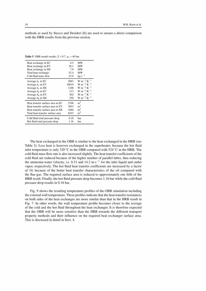
Fig. 9 shows the resulting temperature profiles of the OBB simulation includingthe external wall temperature. These profiles indicate that the heat transfer resistanceson both sides of the heat exchanger are more similar than that in the HRB result inFig. 7. In other words, the wall temperature profile becomes closer to the averageof the cold and the hot fluid throughout the heat exchanger. It is therefore expectedthat the OBB will be more sensitive than the HRB towards the different transportproperty methods and their influence on the required heat exchanger surface area.This is discussed in detail in Sect. 4.


0 10 20 30 40 50 600

50

100

150

200

250

300

350

Heat flow rate, MW

Te

mp

era

ture

, oC

Cold fluid

Hot fluid

Tube wall

0 10 20 30 40 50 600

50

100

150

200

250

300

350

Heat flow rate, MW

Te

mp

era

ture

, oC

Fig. 9 OBB temperature profiles as function of heat flow rate; Z=0.7, pc =40 bar

3.4 Convergence

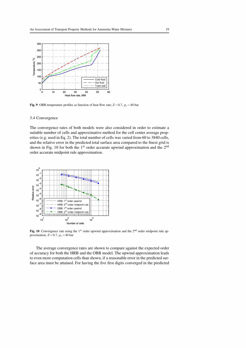
The convergence rates of both models were also considered in order to estimate asuitable number of cells and approximative method for the cell center average prop-erties (e.g. used in Eq. 2). The total number of cells was varied from 60 to 3840 cells,and the relative error in the predicted total surface area compared to the finest grid isshown in Fig. 10 for both the 1st order accurate upwind approximation and the 2nd

order accurate midpoint rule approximation.

101

102

103

10−9

10−8

10−7

10−6

10−5

10−4

10−3

10−2

10−1

100

Number of cells

Re

lative

err

or

HRB: 1st order upwind

HRB: 2nd

order midpoint rule

OBB: 1st order upwind

OBB: 2nd

order midpoint rule

101

102

103

10−9

10−8

10−7

10−6

10−5

10−4

10−3

10−2

10−1

100

Number of cells

Re

lative

err

or

Fig. 10 Convergence rate using the 1st order upwind approximation and the 2nd order midpoint rule ap-proximation, Z=0.7, pc=40 bar

The average convergence rates are shown to compare against the expected orderof accuracy for both the HRB and the OBB model. The upwind approximation leadsto even more computation cells than shown, if a reasonable error in the predicted sur-face area must be attained. For having the five first digits converged in the predicted


Table 6 HRB highest and lowest predicted areas and differences; Z=0.7, pc =40 bar

Viscosity Thermal conductivity Total Area DifferenceLiquid Vapor Liquid Vapor [m2] [%]

Stecco and Desideri [6] Wilke [21] Jamieson et al. [28] Mason and Saxena [25] 41196 1.48Stecco and Desideri [6] Wilke [21] Jamieson et al. [28] Mole-average 41195 1.48Stecco and Desideri [6] Chung et al. [17, 18] Jamieson et al. [28] Mason and Saxena [25] 41171 1.42Stecco and Desideri [6] Chung et al. [17, 18] Jamieson et al. [28] Mole-average 41170 1.41

Hdb Kältetechnik [24] Reichenberg [20] El-Sayed [11] Mason and Saxena [25] 40072 -1.29Hdb Kältetechnik [24] Reichenberg [20] El-Sayed [11] Mole-average 40071 -1.29Hdb Kältetechnik [24] Chung et al. [17, 18] El-Sayed [11] Chung et al. [17, 18] 40050 -1.34Hdb Kältetechnik [24] Reichenberg [20] El-Sayed [11] Chung et al. [17, 18] 40045 -1.36

surface area and using the midpoint rule approximation, we must choose at least 1000cells. For that reason, we used 2000 cells in all the simulations herein to be certainthat the predicted areas are converged.

4 Results

In this section, the influence of the transport property methods on the predicted heattransfer surface area is reported for both the HRB and the OBB. Three methods fromSect. 2.1 to 2.4 each (Figs. 2 to 5), i.e. 12 methods in total, are simulated for allcombinations. The Chung et al. [17, 18] composition-averaged error methods wereexcluded for the vapor viscosity and the thermal conductivity, because these methodsare more computationally intensive than all other methods and therefore not consid-ered to be beneficial for numerical simulation and design. Additionally, coincidingmethods were excluded for the liquid viscosity and thermal conductivity, namely themethods by El-Sayed [11] and Filippov [27], respectively.

4.1 HRB Results

Table 6 shows the four highest and lowest predicted areas for the HRB at an ammoniamass fraction and cold fluid pressure of 0.7 and 40 bar, respectively. Additionally, thearea difference with respect to the mean area (∆At/At) is given. Referring to Figs. 2 to5, the general trend in these results is that an increased thermal conductivity decreasesthe predicted area, while an increased viscosity increases the predicted area. Thisobservation may be explained by reviewing the simple single phase Dittus-Boelterequation [42], for which the heat transfer coefficient is isolated

h =Nuk

d=CRemPrn k

d

= C

(

Gd

µ

)m(cpµ

k

)n k

d

= f(

µn−m,k1−n, . . .)

(6)

where m=0.8, n=0.4, and C is a constant. Thus the exponent of viscosity µ is neg-ative while that of thermal conductivity k is positive in the computation of the single


phase heat transfer coefficient. The boiling two-phase flow heat transfer coefficient ismore complex to analyze similarly. However, the same trend should be expected atleast for the convective boiling contribution.

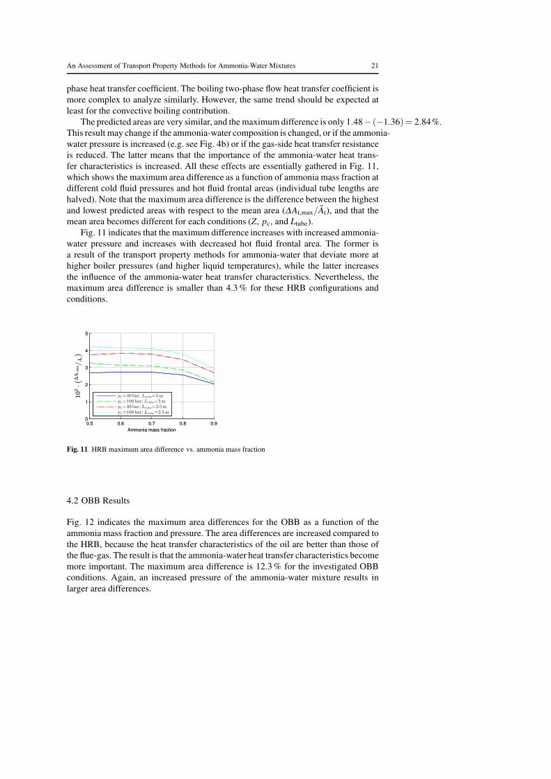
The predicted areas are very similar, and the maximum difference is only 1.48− (−1.36)= 2.84%.This result may change if the ammonia-water composition is changed, or if the ammonia-water pressure is increased (e.g. see Fig. 4b) or if the gas-side heat transfer resistanceis reduced. The latter means that the importance of the ammonia-water heat trans-fer characteristics is increased. All these effects are essentially gathered in Fig. 11,which shows the maximum area difference as a function of ammonia mass fraction atdifferent cold fluid pressures and hot fluid frontal areas (individual tube lengths arehalved). Note that the maximum area difference is the difference between the highestand lowest predicted areas with respect to the mean area (∆At,max/At), and that themean area becomes different for each conditions (Z, pc, and Ltube).

Fig. 11 indicates that the maximum difference increases with increased ammonia-water pressure and increases with decreased hot fluid frontal area. The former isa result of the transport property methods for ammonia-water that deviate more athigher boiler pressures (and higher liquid temperatures), while the latter increasesthe influence of the ammonia-water heat transfer characteristics. Nevertheless, themaximum area difference is smaller than 4.3 % for these HRB configurations andconditions.

0.5 0.6 0.7 0.8 0.9

0

1

2

3

4

5


102·

(

∆A

t,m

ax/A

t

)

pc=40 bar; Ltube=5m

pc=100 bar; Ltube=5m

pc=40 bar; Ltube=2.5 mpc=100 bar; Ltube=2.5 m

0.5 0.6 0.7 0.8 0.9

0

1

2

3

4

5


102·

(

∆A

t,m

ax/A

t

)

Fig. 11 HRB maximum area difference vs. ammonia mass fraction

4.2 OBB Results

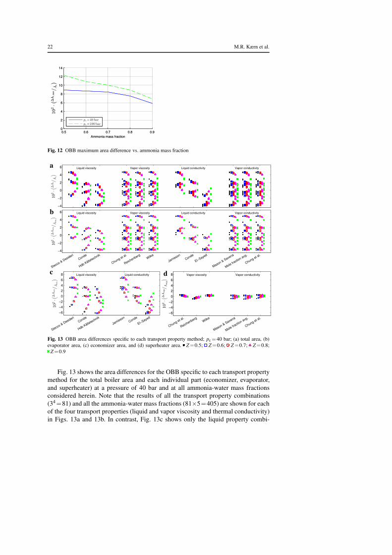
Fig. 12 indicates the maximum area differences for the OBB as a function of theammonia mass fraction and pressure. The area differences are increased compared tothe HRB, because the heat transfer characteristics of the oil are better than those ofthe flue-gas. The result is that the ammonia-water heat transfer characteristics becomemore important. The maximum area difference is 12.3 % for the investigated OBBconditions. Again, an increased pressure of the ammonia-water mixture results inlarger area differences.


0.5 0.6 0.7 0.8 0.9

0

2

4

6

8

10

12

14


102·

(

∆A

t,m

ax/A

t

)

pc=40 bar

pc=100 bar

0.5 0.6 0.7 0.8 0.9

0

2

4

6

8

10

12

14


102·

(

∆A

t,m

ax/A

t

)

Fig. 12 OBB maximum area difference vs. ammonia mass fraction

−4

−2

0

2

4

6

Stecco & Desideri

Conde

Hdb Kältetechnik

Chung et al.

ReichenbergWilke

Jamieson

Conde

El−Sayed

Mason & Saxena

Mole fractio

n avg.

Chung et al.

Liquid viscosity Vapor viscosity Liquid conductivity Vapor conductivity

102·

(

∆A

t/A

t

)

−4

−2

0

2

4

6

Stecco & Desideri

Conde

Hdb Kältetechnik

Chung et al.

ReichenbergWilke

Jamieson

Conde

El−Sayed

Mason & Saxena

Mole fractio

n avg.

Chung et al.

Liquid viscosity Vapor viscosity Liquid conductivity Vapor conductivity

102·

(

∆A

eva/A

eva

)

−6

−4

−2

0

2

4

6

8

Stecco & Desideri

Conde

Hdb Kältetechnik

Jamieson

Conde

El−Sayed

Liquid viscosity Liquid conductivity

102·

(

∆A

eco/A

eco

)

−6

−4

−2

0

2

4

6

8

Chung et al.

ReichenbergWilke

Mason & Saxena

Mole fractio

n avg.

Chung et al.

Vapor viscosity Vapor conductivity

102·

(

∆Asup/Asup

)

a

b

c d

Fig. 13 OBB area differences specific to each transport property method; pc =40 bar; (a) total area, (b)evaporator area, (c) economizer area, and (d) superheater area. Z=0.5; Z=0.6; Z=0.7; Z=0.8;

Z=0.9

Fig. 13 shows the area differences for the OBB specific to each transport propertymethod for the total boiler area and each individual part (economizer, evaporator,and superheater) at a pressure of 40 bar and at all ammonia-water mass fractionsconsidered herein. Note that the results of all the transport property combinations(34=81) and all the ammonia-water mass fractions (81×5=405) are shown for eachof the four transport properties (liquid and vapor viscosity and thermal conductivity)in Figs. 13a and 13b. In contrast, Fig. 13c shows only the liquid property combi-


nations (32×5= 45), while Fig. 13d shows only the vapor property combinations(32×5=45).

Fig. 13d indicates that the vapor transport property methods have little influenceon the required heat transfer surface area (≈1-2 %) of the superheater. This fact isalso indicated in Figs. 13a and 13b for the total and evaporator area, respectively.Here the area differences do not change much when changing the vapor transportproperty method.

On the other hand, the liquid transport property methods show larger area differ-ences as indicated in Fig. 13c for the economizer. These area differences are smallerfor the total and evaporator area (Figs. 13a and 13b), however they show a similartrend. Hence, the results in Fig. 13 suggest that the liquid properties have the highestimpact on the heat exchanger area estimation.

The trend in the results is the same for the 100 bar conditions, and also the samefor the HRB simulations; i.e. the liquid property methods matter the most. Fig. 13aindicates that the highest boiler area is achieved when the liquid viscosity method byStecco and Desideri [6] and the liquid conductivity method by Jamieson et al. [28]are used. This is the same result as indicated in Table 6 for the HRB. Furthermore,the lowest boiler area in Fig. 13a (at Z = 0.7) occurs when using the liquid viscos-ity method proposed in Handbuch der Kältetechnik [24] and the liquid conductivitymethod by El-Sayed [11]. Again, the same result is suggested in Table 6 for the HRB.

5 Discussion

The work by Thorin [9] suggests that the use of different transport property methodsmay lead to differences as much as 10 % in the predicted heat transfer area. It shouldbe noted that the 10 % refers to individual heat exchangers and not the HRB or thetotal heat transfer area in the author’s Kalina cycle configuration. Only 0.64 % areadifference was associated with the HRB, while half of the total area was used for thatcomponent. Moreover, 3 % area difference was associated with the total heat transferarea.

The current comparison shows a much higher difference for the HRB than in thework by Thorin [9] (4.3% ≫ 0.64%). Thorin [9] used an ammonia-water pressureof 108 bar. However, no information was given on the heat exchanger geometry suchas fins and frontal areas. The latter issue makes it difficult to compare the resultsdirectly. Additionally, Thorin [9] used a constant boiling heat transfer coefficient of10 kW·m−2·K−1.

The HRB is usually gas-side controlled, reducing the effects of the ammonia-water heat transfer characteristics. On the other hand, the heat transfer resistanceson both fluid sides are more evenly distributed. Nevertheless, the influence of usingdifferent transport property methods resulted in less than 12.3 % predicted area differ-ence during the OBB design. In the light of typical uncertainties in the heat transfercorrelations for both single and two-phase flows, the result is encouraging, becauseit indicates that the use of different ammonia-water transport property methods has aminor significance during heat exchanger design. The vapor methods showed nearlysimilar results, while the liquid methods appeared to have higher significance. It is


however believed that the recuperators in Kalina cycles may show larger area dif-ferences, because these have the ammonia-water mixtures on both sides of the heatexchanger.

For the above reasons, it cannot be claimed that some methods necessarily aremore appropriate to use than others. Nevertheless, a few preliminary guidelines areprovided in the following. For the liquid viscosity and thermal conductivity, the au-thors’ suggest the use of the methods by Conde-Petit [1]. These methods comparethe best with the experimental data in Fig. 3a, 5a and 5b, although the thermal con-ductivity data show a large scatter. Furthermore, these methods are smooth and con-tinuous in the investigated temperature range. For the vapor viscosity and thermalconductivity, the authors’ suggest use of the methods by Wilke [21] and Mason andSaxena [25], tentatively, when a dynamic simulation is not performed. For dynamicsimulation, a continuous first derivative is imperative, and the user should choose thecorresponding state methods by Chung et al. [17, 18]. The methods by Wilke [21] andMason and Saxena [25] were also proposed by Conde-Petit [1] and El-Sayed [11].

Many boiling heat transfer correlations have been proposed for binary mixtures,and these should also be assessed with regards to their significance on the predictedheat transfer area during design to achieve a full evaluation of ammonia-water mix-ture effects. These heat transfer correlations typically suggest high degradation forwide-boiling mixtures, thus leading to a higher heat transfer surface area. In thisstudy, the Shah [38] correlation was used including mixture properties. The corre-lation was not specially developed for mixtures, but has been shown to agree rea-sonably well for refrigerant mixtures [7]. However, it does not include the nucleateboiling suppression due to mass diffusion. It is a topic of interest in future work ofour research.

6 Conclusion

This paper presents a systematic numerical analysis of several transport propertymethods applicable to ammonia-water mixtures in an attempt to quantify their in-dividual influence during heat exchanger design. Two design studies related to theuse of the Kalina cycle were considered for this purpose: a flue-gas-based heat recov-ery boiler (HRB) for a combined cycle power plant and a hot-oil-based boiler (OBB)for a solar thermal power plant.

From the heat exchanger design simulations, it may be concluded that the trans-port property methods resulted in minor differences in the predicted heat transferarea. The maximum predicted heat transfer area differences were 4.3 % and 12.3 %for the HRB and the OBB, respectively. These simulations were performed at variousammonia-mass fractions (0.5 to 0.9) and pressures (40 to 100 bar). Additionally, thegas-side heat transfer resistance was reduced by halving the gas-side frontal area forthe HRB.

The design simulations indicate that the liquid transport property methods resultin more of the area differences than the vapor transport property methods. Addition-ally, the area difference increases at higher boiler pressures.


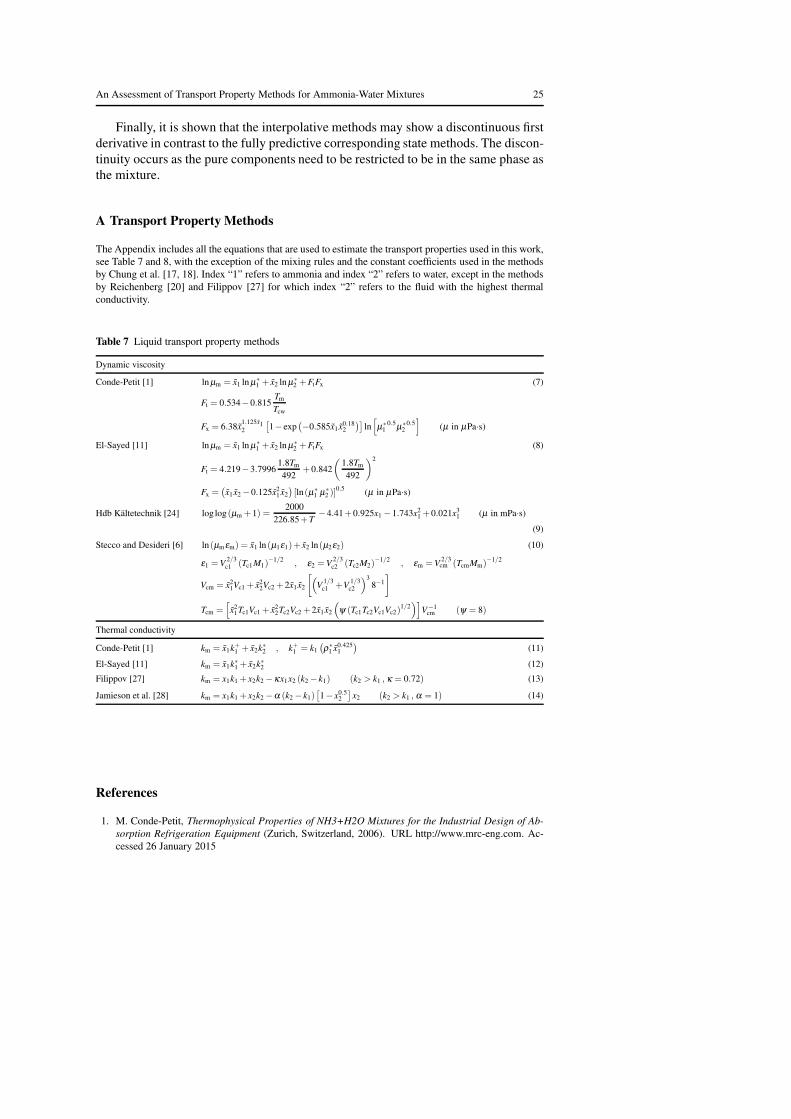
Finally, it is shown that the interpolative methods may show a discontinuous firstderivative in contrast to the fully predictive corresponding state methods. The discon-tinuity occurs as the pure components need to be restricted to be in the same phase asthe mixture.

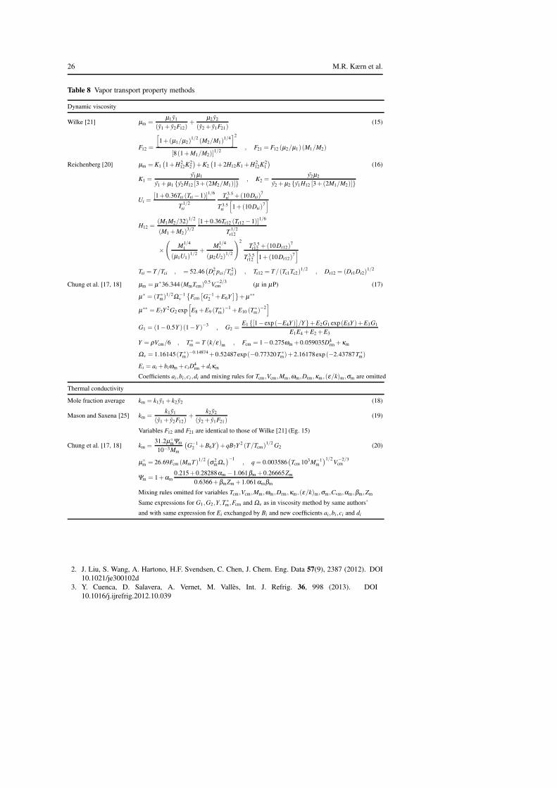
A Transport Property Methods

The Appendix includes all the equations that are used to estimate the transport properties used in this work,see Table 7 and 8, with the exception of the mixing rules and the constant coefficients used in the methodsby Chung et al. [17, 18]. Index “1” refers to ammonia and index “2” refers to water, except in the methodsby Reichenberg [20] and Filippov [27] for which index “2” refers to the fluid with the highest thermalconductivity.

Table 7 Liquid transport property methods

Dynamic viscosity

Conde-Petit [1] ln µm = x1 ln µ∗1 + x2 ln µ∗

2 +FtFx (7)

Ft = 0.534−0.815Tm

Tcw

Fx = 6.38x1.125x12

[

1− exp(

−0.585x1 x0.182

)]

ln[

µ∗1

0.5µ∗2

0.5]

(µ in µPa·s)

El-Sayed [11] ln µm = x1 ln µ∗1 + x2 ln µ∗

2 +FtFx (8)

Ft = 4.219−3.79961.8Tm

492+0.842

(

1.8Tm

492

)2

Fx =(

x1 x2 −0.125x21 x2)

[ln(µ∗1 µ∗

2 )]0.5 (µ in µPa·s)

Hdb Kältetechnik [24] log log (µm +1) =2000

226.85+T−4.41+0.925x1 −1.743x2

1 +0.021x31 (µ in mPa·s)

(9)

Stecco and Desideri [6] ln (µmεm) = x1 ln (µ1ε1)+ x2 ln(µ2ε2) (10)

ε1 =V2/3c1 (Tc1M1)

−1/2 , ε2 =V2/3c2 (Tc2M2)

−1/2 , εm =V2/3cm (TcmMm)

−1/2

Vcm = x21Vc1 + x2

2Vc2 +2x1 x2

[

(

V1/3c1 +V

1/3c2

)38−1]

Tcm =[

x21Tc1Vc1 + x2

2Tc2Vc2 +2x1 x2

(

ψ (Tc1Tc2Vc1Vc2)1/2)]

V−1cm (ψ = 8)

Thermal conductivity

Conde-Petit [1] km = x1k+1 + x2k∗2 , k+1 = k1(

ρ∗1 x0.425

1

)

(11)

El-Sayed [11] km = x1k∗1 + x2k∗2 (12)

Filippov [27] km = x1k1 + x2k2 −κx1x2 (k2 − k1) (k2 > k1 , κ = 0.72) (13)

Jamieson et al. [28] km = x1k1 + x2k2 −α (k2 − k1)[

1− x0.52

]

x2 (k2 > k1 , α = 1) (14)

References

1. M. Conde-Petit, Thermophysical Properties of NH3+H2O Mixtures for the Industrial Design of Ab-

sorption Refrigeration Equipment (Zurich, Switzerland, 2006). URL http://www.mrc-eng.com. Ac-cessed 26 January 2015


Table 8 Vapor transport property methods

Dynamic viscosity

Wilke [21] µm =µ1 y1

(y1 + y2F12)+

µ2 y2

(y2 + y1F21)(15)

F12 =

[

1+(µ1/µ2)1/2 (M2/M1)

1/4]2

[8(1+M1/M2)]1/2

, F21 = F12 (µ2/µ1)(M1/M2)

Reichenberg [20] µm = K1(

1+H212K2

2

)

+K2(

1+2H12K1 +H212K2

1

)

(16)

K1 =y1µ1

y1 +µ1 y2H12 [3+(2M2/M1)], K2 =

y2µ2

y2 +µ2 y1H12 [3+(2M1/M2)]

Ui =[1+0.36Tri (Tri −1)]1/6

T1/2

ri

T 3.5ri +(10Dri)

7

T 3.5ri

[

1+(10Dri)7]

H12 =(M1M2/32)1/2

(M1 +M2)3/2

[1+0.36Tr12 (Tr12 −1)]1/6

T1/2

r12

×

(

M1/41

(µ1U1)1/2

+M

1/42

(µ2U2)1/2

)2T 3.5

r12 +(10Dr12)7

T 3.5r12

[

1+(10Dr12)7]

Tri = T/Tci , = 52.46(

D2i pci/T 2

ci

)

, Tr12 = T/(Tc1Tc2)1/2 , Dr12 = (Dr1Dr2)

1/2

Chung et al. [17, 18] µm = µ∗36.344(MmTcm)0.5

V−2/3cm (µ in µP) (17)

µ∗ = (T ∗m)

1/2Ω−1v

Fcm[

G−12 +E6Y

]

+µ∗∗

µ∗∗ = E7Y 2G2 exp[

E8 +E9 (T∗

m)−1 +E10 (T

∗m)

−2]

G1 = (1−0.5Y )(1−Y )−3 , G2 =E1 [1− exp (−E4Y )]/Y+E2G1 exp (E5Y )+E3G1

E1E4 +E2 +E3

Y = ρVcm/6 , T ∗m = T (k/ε)m , Fcm = 1−0.275ωm +0.059035D4

rm +κm

Ωv = 1.16145(T ∗m)

−0.14874 +0.52487exp (−0.77320T ∗m)+2.16178exp (−2.43787T ∗

m)

Ei = ai +biωm + ciD4rm +diκm

Coefficients ai,bi,ci ,di and mixing rules for Tcm,Vcm,Mm,ωm,Drm,κm,(ε/k)m,σm are omitted

Thermal conductivity

Mole fraction average km = k1y1 + k2 y2 (18)

Mason and Saxena [25] km =k1y1

(y1 + y2F12)+

k2 y2

(y2 + y1F21)(19)

Variables F12 and F21 are identical to those of Wilke [21] (Eg. 15)

Chung et al. [17, 18] km =31.2µ

mΨm

10−3Mm

(

G−12 +B6Y

)

+qB7Y 2 (T/Tcm)1/2

G2 (20)

µm = 26.69Fcm (MmT )1/2 (σ2

mΩv)−1

, q = 0.003586(

Tcm 103M−1m

)1/2V

−2/3cm

Ψm = 1+αm0.215+0.28288αm −1.061βm +0.26665Zm

0.6366+βmZm +1.061αmβm

Mixing rules omitted for variables Tcm,Vcm,Mm,ωm,Drm,κm,(ε/k)m,σm,Cvm,αm,βm,Zm

Same expressions for G1,G2 ,Y,T∗

m ,Fcm and Ωv as in viscosity method by same authors’

and with same expression for Ei exchanged by Bi and new coefficients ai,bi,ci and di

2. J. Liu, S. Wang, A. Hartono, H.F. Svendsen, C. Chen, J. Chem. Eng. Data 57(9), 2387 (2012). DOI10.1021/je300102d

3. Y. Cuenca, D. Salavera, A. Vernet, M. Vallès, Int. J. Refrig. 36, 998 (2013). DOI10.1016/j.ijrefrig.2012.10.039


4. F.N. Shamsetdinov, Z.I. Zaripov, I.M. Abdulagatov, M.L. Huber, F.M. Gumerov, F.R. Gabitov, A.F.Kazakov, Int. J. Refrig. 36, 1347 (2013). DOI 10.1016/j.ijrefrig.2013.02.008

5. E.W. Lemmon, M.L. Huber, M.O. Mclinden, NIST Standard Reference Database 23: Reference Fluid

Thermodynamic and Transport Properties – REFPROP 9.12 (National Institute of Standards andTechnology, Boulder, Colorado, USA, 2013)

6. S.S. Stecco, U. Desideri, J. Eng. Gas Turbines Power 114(4), 701 (1992). DOI doi:10.1115/1.29066457. D.S. Jung, M. McLinden, R. Radermacher, D. Didion, Int. J. Heat Mass Transf. 32(9), 1751 (1989).

DOI 10.1016/0017-9310(89)90057-48. G.P. Celata, M. Cumo, T. Setaro, Exp. Therm. Fluid Sci. 9(4), 367 (1994). DOI 10.1016/0894-

1777(94)90015-99. E. Thorin, Int. J. Thermophys. 22(1), 201 (2001). DOI 10.1023/A:1006745100278

10. R. Tillner-Roth, D. Friend, J. Phys. Chem. Ref. data 27(1), 63 (1998). DOIhttp://dx.doi.org/10.1063/1.556015

11. Y. El-Sayed, Winter Annu. Meet. Am. Soc. Mech. Eng. pp. 19–24 (1988)12. A. Modi, F. Haglind, Appl. Therm. Eng. 65(1-2), 201 (2014). DOI

10.1016/j.applthermaleng.2014.01.01013. E.W. Lemmon, Private communication (National Institute of Standards and Technology, Boulder,

Colorado, USA, 2013)14. A. Modi, F. Haglind, Appl. Therm. Eng. 76, 196 (2015). DOI 10.1016/j.applthermaleng.2014.11.04715. C.L. Sassen, R.A.C. van Kwartel, H.J. van Der Kooi, J. de Swaan Arons, J. Chem. Eng. Data 35, 140

(1990). DOI 10.1021/je00060a01316. B.E. Poling, J.M. Prausnitz, J.P. O’Connell, The Properties of Gases and Liquids, 5th edn. (McGraw-

Hill, New York, USA, 2001)17. T.H. Chung, L.L. Lee, K.E. Starling, Ind. & Eng. Chem. Fundam. 23, 8 (1984). DOI

10.1021/i100013a00218. T.H. Chung, M. Ajlan, L.L. Lee, K.E. Starling, Ind. & Eng. Chem. Res. 27(4), 671 (1988). DOI

10.1021/ie00076a02419. A.S. Teja, P. Rice, Ind. & Eng. Chem. Fundam. 20(1), 77 (1981). DOI 10.1021/i100001a01520. D. Reichenberg, New simplified methods for the estimation of the viscosities of gas mixtures at moder-

ate pressures (National Physical Laboratory, Division of Chemical Standards, East Kilbride, Glasgow,Scotland, 1977)

21. C.R. Wilke, J. Chem. Phys. 18(4), 517 (1950). DOI 10.1063/1.174767322. M.J.W. Frank, J.A.M. Kuipers, W.P.M. van Swaaij, J. Chem. Eng. Data 41(2), 297 (1996). DOI

10.1021/je950157k23. G. Pinewitsch. Cholodilnaja Technika 20(3), 30 (1948). Reproduced in Kältetechnik 2(2), 29 (1950)24. R. Plank, F. Steimle, K. Stephan, Handbuch der Kältetechnik. - 6B: Wärmeaustauscher (Springer,

Berlin, Germany, 1988)25. E.A. Mason, S.C. Saxena, Phys. Fluids 1(5), 361 (1958). DOI 10.1063/1.172435226. A. Baranov, B. Churagulov, A. Kalina, F. Sharikov, A. Zharov, A. Yoroslavtsev, in Rep. Work. Thermo-

phys. Prop. Ammon. Mix., ed. by W. Friend, D.G., Haynes (NISTIR 5059, Boulder, Colorado, USA,1997), pp. 59–67

27. L. Filippov, Ser. Fiz. Mat. Estestv. Nauk 10, 67 (1955)28. D.T. Jamieson, J.B. Irving, J.S. Tudhope, Liquid thermal conductivity. A data survey to 1973 (Edin-

burgh, Scotland, 1975)29. Dymola 2014. Dynamic Modeling Laboratory, Dassault Systemes AB, Research Park Ideon SE-223

70, Lund, Sweden (2014)30. J. Wronski, M.R. Kærn, H. Francke, REFPROP2Modelica (Technical University of Denmark and

GFZ Potsdam, 2014). URL https://github.com/jowr/REFPROP2Modelica. Accessed 26 January 201531. M.B. Ibrahim, R.M. Kovach, Energy 18(9), 961 (1993). DOI 10.1016/S0360-5442(06)80001-032. P. Nag, A. Gupta, Appl. Therm. Eng. 18(6), 427 (1998). DOI 10.1016/S1359-4311(97)00047-133. D.E. Briggs, E.H. Young, Chem. Eng. Prog. Symp. Ser. 59(41), 1 (1963)34. R.K. Shah, D.P. Sekulic, Fundamentals of heat exchanger design (John Wiley & Sons, Hoboken, New

Jersey, USA, 2003)35. K.K. Robinson, D.E. Briggs, Chem. Eng. Prog. Symp. Ser. 62(64), 177 (1966)36. V. Gnielinski, Int. Chem. Eng. 16, 359 (1976)37. H. Blasius, in Mitteilungen über Forschungsarbeiten auf dem Gebiete des Ingenieurwesens 131

(Springer, Berlin, Germany, 1913), pp. 1–4138. M.M. Shah, ASHRAE Trans. 88, 185 (1982)


39. H. Müller-Steinhagen, K. Heck, Chem. Eng. Process. Process Intensif. 20, 297 (1986)40. Solutia Inc., Therminol 66, High performance highly stable heat transfer fluid (2014). URL

http://twt.mpei.ac.ru. Accessed 26 January 201541. J. Taborek, in Heat Exch. Des. Handb., ed. by G.F. Hewitt (Begell House, New York, USA, 1998),

chap. 3, pp. 3.3.3–1 – 3.3.11–542. F.W. Dittus, L.M.K. Boelter, Univ. Calif. Publ. Eng. 2(13), 443 (1930)

Documents

An Assessment of Transport Property Estimation Methods for ...orbit.dtu.dk/files/110304601/Nakai_et_al_abstract.pdf · International Journal of Thermophysics manuscript No. (will