AN ASSESSMENT OF THE IMPACTS OF FUTURE CO2 AND CLIMATE ON

CALIFORNIAN AGRICULTURE

A Report From: California Climate Change Center

Prepared By: Dennis Baldocchi and Simon Wong University of California, Berkeley

WH

ITE

PAPE

R

DISCLAIMER This report was prepared as the result of work sponsored by the California Energy Commission (Energy Commission) and the California Environmental Protection Agency (Cal/EPA). It does not necessarily represent the views of the Energy Commission, Cal/EPA, their employees, or the State of California. The Energy Commission, Cal/EPA, the State of California, their employees, contractors, and subcontractors make no warrant, express or implied, and assume no legal liability for the information in this report; nor does any party represent that the uses of this information will not infringe upon privately owned rights. This report has not been approved or disapproved by the California Energy Commission or Cal/EPA, nor has the California Energy Commission or Cal/EPA passed upon the accuracy or adequacy of the information in this report.

Arnold Schwarzenegger, Governor March 2006 CEC-500-2005-187-SF

i

Acknowledgements

We acknowledge support from the California Energy Commission and Environmental Protection Agency and the California Agricultural Extension Service. We thank the California Climate Archive for its provision of climate data, as well as the original data sources from the CIMIS project and the National Climate Center Coop network. We thank Ed Maurer, Mary Tyree, and Andrew Gutierrez for supplying the climate projection scenarios and Michael Hanemann and Guido Franco for their guidance and leadership. We thank Dr. Edward Vine of the California Institute for Energy and Environment for managing the peer review process that was conducted for this paper. Finally, we thank Rick Synder, Lloyd Wilson, David Wolfe, and Steve Shaffer for providing helpful and expert reviews of this report.

ii

Preface

The Public Interest Energy Research (PIER) Program supports public interest energy research and development that will help improve the quality of life in California by bringing environmentally safe, affordable, and reliable energy services and products to the marketplace.

The PIER Program, managed by the California Energy Commission (Energy Commission), annually awards up to $62 million to conduct the most promising public interest energy research by partnering with Research, Development, and Demonstration (RD&D) organizations, including individuals, businesses, utilities, and public or private research institutions.

PIER funding efforts are focused on the following RD&D program areas:

• Buildings End-Use Energy Efficiency

• Energy-Related Environmental Research

• Energy Systems Integration

• Environmentally Preferred Advanced Generation

• Industrial/Agricultural/Water End-Use Energy Efficiency

• Renewable Energy Technologies

The California Climate Change Center (CCCC) is sponsored by the PIER program and coordinated by its Energy-Related Environmental Research area. The Center is managed by the California Energy Commission, Scripps Institution of Oceanography at the University of California at San Diego, and the University of California at Berkeley. The Scripps Institution of Oceanography conducts and administers research on climate change detection, analysis, and modeling; and the University of California at Berkeley conducts and administers research on economic analyses and policy issues. The Center also supports the Global Climate Change Grant Program, which offers competitive solicitations for climate research.

The California Climate Change Center Report Series details ongoing Center-sponsored research. As interim project results, these reports receive minimal editing, and the information contained in these reports may change; authors should be contacted for the most recent project results. By providing ready access to this timely research, the Center seeks to inform the public and expand dissemination of climate change information; thereby leveraging collaborative efforts and increasing the benefits of this research to California’s citizens, environment, and economy.

For more information on the PIER Program, please visit the Energy Commission’s website www.energy.ca.gov/pier/ or contact the Energy Commission at (916) 654-5164.

iii

Table of Contents

Preface.. ................................................................................................................................................ ii Abstract ................................................................................................................................................v 1.0 Introduction ..........................................................................................................................1 2.0 Literature Synthesis .............................................................................................................3

2.1. Temperature ....................................................................................................................3 2.2. Carbon Dioxide Concentration.....................................................................................8

3.0 Water Use..............................................................................................................................11 4.0 Contemporary Temperature Trends .................................................................................17 5.0 Conclusions...........................................................................................................................29 6.0 References .............................................................................................................................30

List of Figures

Figure 1. Theoretical variations in latent heat exchange and stomatal conductance of a C3 leaf with varying CO2. A coupled leaf energy balance-photosynthesis model that considers the effect of CO2 is used to make the calculations (Baldocchi, 1994; Baldocchi et al., 1999). Computations assumed global radiation was 1000 W m-2, air temperature was 25°C (77°F), wind speed was 1.0 m s-1 and vapor pressure was 1.5 kilopascals (kPa). .......................................................................................................... 12

Figure 2. Relationship between normalized evaporation and canopy resistance. Data are from a variety of crops and native vegetation. (Baldocchi et al., 1997). The figure is updated with a new set of data from a Californian oak-grass savanna. .................... 13

Figure 3. Computation of evaporation from a California walnut orchard. Simulations are based on the CANVEG model. The top panel shows the seasonal course of daily average latent heat exchange for 2003 weather conditions. The bottom panel shows the difference in evaporation on the assumption that air temperature increases 3°C and CO2 is at 500 ppm........................................................................................................ 15

Figure 4. Trend in accumulated chill degree hours at Brentwood, California, between 1986 and 2005. The slope indicates a reduction of 422 chill degree hours per year. The coefficient of variation indicates that 48% of the variance in chill degree hours is explained by time. .............................................................................................................. 20

iv

Figure 5. Schematic of the mean diurnal temperature course. Line a is 6 hours in length, line b is the distance between average and reference temperatures, line c is between the reference and minimum temperature, and line d is one-half the duration that temperature is below the reference temperature. .......................................................... 21

Figure 6. Comparison between accumulated chill hours using hourly and maximum and minimum temperature measurements for Zamora, California. .................................. 22

Figure 7. Long-term trend in accumulated chill degree hours at Angwin, California. .... 23

Figure 8. Map of long-term trends in the change in winter chill accumulation (degree hours) over the course of the dormant period. Data are derived from the California Climate Archive. ................................................................................................................. 24

Figure 9. Current and future projections of chill degree hour accumulation for three sites up and down the Central Valley (Red Bluff, Davis, and Fresno). Climate projections were computed to 2100 for scenarios B1 and A2. .......................................................... 25

Figure 10. Current and future projections of chill hour accumulation for three sites up and down the Central Valley (Red Bluff, Davis, and Fresno). Climate projections were computed to 2100 for scenarios B1 and A2. .......................................................... 27

Figure 11. Probability distribution of sunlit leaf temperature for contemporary and future climate conditions................................................................................................... 28

List of Tables

Table 1. Summary of positive and negative effects on California agriculture by associated elevated CO2 and regional warming .............................................................. 4

Table 2. Fractional change in yield (% change /100) relative to current production in San Joaquin Valley for eight possible changes in precipitation and temperature (Adams et al., 2001) ............................................................................................................................. 7

Table 3. Estimates of regional evaporation for the western Pacific region of the United States. Scenarios based on the Canadian Climate and Hadley Centre climate models are used. (Izaurralde et al., 2003)..................................................................................... 16

Table 4. Number of hours below a threshold temperature, e.g., 7°C for dormancy. Australasian Tree Crops Source Book http://www.aoi.com.au/atcros/LM.htm. .. 17

v

Abstract

This report evaluates how global warming and the associated rise in atmospheric CO2 will affect several facets of agriculture in California―crop production, water use, and crop phenology. Our analysis is based on a survey of peer-reviewed literature, an analysis of trends in crop-related climate variables, and simulations with a biophysical model, CANVEG.

Our survey of the pertinent literature reveals a combination of positive and negative effects of warming and elevated CO2 on crop production. Elevated CO2 gives crops a spurt in growth, as photosynthesis responds positively to extra CO2. But enhanced photosynthesis is not sustained, as photosynthesis eventually experiences down-regulation. Elevated CO2 also causes stomata to close. This effect has favorable implications on water saving by reducing transpiration at the leaf scale. In contrast, larger crops growing in a warmer climate will use more water, at the field scale. Indirect effects of elevated CO2 and warming on agriculture will include a lengthening of the growing and transpiration seasons, stimulation of weeds and more insect pests. Pollination will be negatively impacted if warming causes asynchronization between flowering and the life cycle of insect pollinators.

An assessment of water use for a walnut orchard for future conditions that are 3°C (5.4°F) warmer and experience 500 parts per million (ppm) of CO2 was produced using the biophysical model CANWALNUT. Computations indicate that the orchard will use an additional 145 millimeters (5.7 inches) of water in the future. Partial stomatal closure in a high-CO2 world increases leaf temperature of sunlit leaves and strengthens the vapor pressure gradient between leaves and the atmosphere.

Fruit trees need 200 to 1200 hours of winter chill to flower. Long-term climate records, measured across the fruit growing region of California, were scrutinized for trends in winter chilling degree-hours and chill hours. Global warming seems to be in motion, as all sites studied are experiencing a negative trend in winter chill accumulation. Calculations of trends in future chill, based on CO2 emission scenarios and use of a global change model, indicate that by 2100, the occurrence of adequate winter chill may be lost for many fruit species. The development of cultivars requiring less winter chill may be one way to circumvent this trend.

1

1.0 Introduction California’s diverse geography and microclimates enables it to serve as a venue for more than 350 field and vegetable, fruit, and nut crops. From the perspective of the United States, California is nearly the sole producer of a large number of desirable fruits and crops. For example, California produces over 95% of the United State’s apricots, almonds, artichokes, figs, kiwis, raisin grapes, olives, cling peaches, dried plums, persimmons, pistachios, olives, and walnuts (California Agricultural Statistics Service, 2003). California’s ability to produce a large and diverse number of crops stems, in part, from the Mediterranean climate that is experienced in many of its interior valleys. There, typical climate conditions include a long growing season with ample sunshine and rainy, cool winters. Moreover, many of the interior valleys experience extended periods of fog during the winter (Suckling and Mitchell, 1988; Underwood et al., 2004). This meteorological occurrence is a key attribute for sustaining a sufficient dormant period for fruit trees (Aron, 1983). Additional factors for producing many unique crops, fruits, and nuts include an ample supply of irrigation water to fertile and arable soils.

California’s cornucopia is predicated on its current climate and its supply and distribution of irrigation water; the latter is mainly derived from the snowpack on the surrounding Cascade and Sierra Nevada mountains, and is stored in dams and distributed via a network of aqueducts and canals. Unfortunately, current climate conditions in California are expected to change over the next 50 to 100 years (Hayhoe et al., 2004). So before we can assess how agriculture may vary in the future we must ask and answer: what will the climate and the supply and demand for irrigation water be in the future? Future climate projections depend upon future patterns of fossil fuel combustion, deforestation, population growth, technological innovations, and future CO2 levels. Global mean CO2 levels are expected to continue rising, and range between 600 and 1000 parts per million (ppm) by 2100 (Friedlingstein et al., 2003; Fung et al., 2005). For perspective, these future values will more than double current CO2 levels (which are near 380 ppm) and pre-industrial levels CO2 levels, which were near 280 ppm (Prentice et al., 2000). Because CO2 is a radiation-absorbing greenhouse gas, its increasing burden in the atmosphere is expected to produce a warmer climate (Manabe and Wetherald, 1975). Climate models that simulate a coupling between the climate and carbon cycle predict a 3°C to 5°C (5.4°F to 9.0°F) increase in the mean global temperature by 2100 (Friedlingstein et al., 2003; Fung et al., 2005). At the regional scale, climate simulations for California predict that a doubling of pre-industrial CO2 levels, from 280 to 560 ppm, will produce up to a 3°C to 4°C (5.4°F to 7.2°F) warming. They also predict a decrease in the extent and amount of winter snowpack on the mountains of California (Hayhoe et al., 2004; Izaurralde et al., 2003; Snyder et al., 2002).

Regional analyzes of climate trends over agricultural regions of California suggest that climate change is already in motion. Feng and Hu (2004) document trends in lengthening of the growing season by about a day per decade over California. They also report that thermal time, heat units that are summed and used to predict phenology and crop growth, are increasing by 30 to 70 growing degree days per decade over California. Nemani et al. (2001) analyzed long term climate records along the coastal region of northern California. They report a warming trend in annual average temperature of over

2

1°C (1.8°F) over 47 years. This warming was associated with a 20 day (d) reduction in the last day of frost occurrence and a 65 d increase in the frost-free growing period. Proxy data, based on the analysis of the springtime advance in the blooming of lilac, provides additional and independent evidence that a warming trend is occurring across the western United States (Cayan et al., 2001). These results indicate that plants are sensing an advance in spring.

This report evaluates the potential consequences of global warming on Californian agriculture. In making this assessment we first distill and synthesize relevant literature on the impacts of climate change on various facets of Californian agriculture. This involves an evaluation on how elevated CO2 and warmer temperatures will affect crop growth, yield, and its associated physiological processes (photosynthesis, respiration, and transpiration). Next we evaluate long-term climate records in the crop growing regions of California to detect any emerging trends on climate indices that relate to crop production. Specifically, we examine trends in accumulated winter chill across the fruit-growing region of California.

3

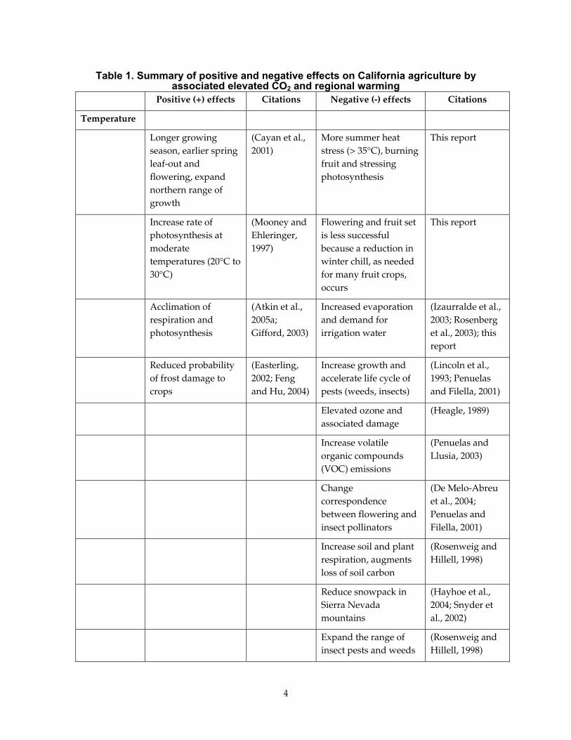
2.0 Literature Synthesis Crops need sunlight, heat, water, carbon dioxide, and nutrients to grow. Changing any of these factors, individually or in combination, with global warming can yield a blend of positive and negative effects on crop production and the physiological processes associated with crop production. These effects are summarized in Table 1 and discussed in greater detail below.

Predicting how crop production, and associated physiological processes, will respond to environmental perturbation is complex. First, many physiological processes (photosynthesis, respiration, transpiration) are non-linear functions of temperature and CO2. Secondly, there are situations when the crop production and physiological processes are dependent upon antecedent conditions, causing them to experience acclimation and down-regulation. In our assessment of how California agriculture could respond to future climate and environmental conditions, we first consider the direct (respiration, photosynthesis, evaporation) and indirect (growing season length, water use) effects of increasing temperature. This analysis is followed by an evaluation of the effects of elevated CO2 on crop production. Direct and indirect effects that co-vary with temperature and CO2 are also discussed. For example, stresses like summertime ozone levels and growth rates of weeds, insect pests, and pathogens will increase with temperature. In addition, threshold effects like flowering and pollination may be threatened if lengthening of the growing season introduces asynchrony between the timing of flowering and the life cycle of important insect pollinators or shortens the length of the dormant period.

2.1. Temperature Crop production is predicated on the condition that photosynthesis outpaces respiration. The enzyme reactions that promote photosynthesis and respiration vary, relative to one another, in their sensitivity to temperature, as defined by the Arrhenius equation (Amthor, 1994). In principle, increasing temperature promotes respiration over assimilation by causing the relative solubility of CO2 versus oxygen and the specificity factor of the enzyme Rubisco (ribulose carboxylase-oxygenase) to decrease (Farquhar et al., 1980; Harley and Tenhunen 1991). High leaf temperatures (exceeding 30°C (86°F) can damage chlorophyll-proteins in the thylakoid membrane, inactivate photosystem II and promote respiration (Harley and Tenhunen 1991).

In general, net carbon assimilation of a leaf will increase with temperature until an optimum is reached—then higher temperatures limit photosynthesis (Bjorkman, 1980; Long, 1985). Furthermore, photosynthesis ceases at extremely high and low temperatures. Most plants cease photosynthesis at temperatures exceeding 50°C (122°F) (Bjorkman, 1980) and temperatures between 0°C and 10°C (32°F to 50°F) tend to be key points for the cessation of photosynthetic activity.

4

Table 1. Summary of positive and negative effects on California agriculture by associated elevated CO2 and regional warming

Positive (+) effects Citations Negative (-) effects Citations

Temperature

Longer growing season, earlier spring leaf-out and flowering, expand northern range of growth

(Cayan et al., 2001)

More summer heat stress (> 35°C), burning fruit and stressing photosynthesis

This report

Increase rate of photosynthesis at moderate temperatures (20°C to 30°C)

(Mooney and Ehleringer, 1997)

Flowering and fruit set is less successful because a reduction in winter chill, as needed for many fruit crops, occurs

This report

Acclimation of respiration and photosynthesis

(Atkin et al., 2005a; Gifford, 2003)

Increased evaporation and demand for irrigation water

(Izaurralde et al., 2003; Rosenberg et al., 2003); this report

Reduced probability of frost damage to crops

(Easterling, 2002; Feng and Hu, 2004)

Increase growth and accelerate life cycle of pests (weeds, insects)

(Lincoln et al., 1993; Penuelas and Filella, 2001)

Elevated ozone and associated damage

(Heagle, 1989)

Increase volatile organic compounds (VOC) emissions

(Penuelas and Llusia, 2003)

Change correspondence between flowering and insect pollinators

(De Melo-Abreu et al., 2004; Penuelas and Filella, 2001)

Increase soil and plant respiration, augments loss of soil carbon

(Rosenweig and Hillell, 1998)

Reduce snowpack in Sierra Nevada mountains

(Hayhoe et al., 2004; Snyder et al., 2002)

Expand the range of insect pests and weeds

(Rosenweig and Hillell, 1998)

5

Table 1. (continued) Positive (+) effects Citations Negative (-) effects Citations

CO2

Increase biomass production

(Ainsworth and Long, 2005; Centritto et al., 1999; Long et al., 2004)

Greater plant respiration, which scales with increased biomass

(Gifford, 2003)

Reduced stomatal conductance, increasing water use efficiency

(Ainsworth and Long, 2005; Long et al., 2004)

Increase the need for fertilizer or nitrogen

(Zavaleta et al., 2003)

Marginal increase in the rate of evaporation for irrigated and closed canopies and C3 crops

This report Increase the absolute need for water

(Izaurralde et al., 2003)

Enhanced insect herbivory

(Lincoln et al., 1993)

Down-regulation of photosynthesis

(Wolfe et al., 1999)

Weeds are benefited more that crops

(Ziska, 2003)

Predicting how photosynthesis will respond to temperature trends is complicated by the fact that the optimum temperature for photosynthesis is very plastic and varies with temperature adaptation and acclimation (Bjorkman, 1980; Long, 1985). Optimum temperatures for desert species can increase from 25°C (77°F) in the spring to near 40°C (104°F) during the summer, or shift if they are grown in cool or hot climates (Larcher, 1975). One literature survey found that the optimum temperature increases by 1°C to 3°C (1.8°F to 5.4°F) for each 5°C (9°F) change in growth temperature (Long, 1985).

Plant respiration rates will approximately double with every 10°C (18°F) increase in temperature (Amthor, 2000). However, short-term responses of respiration to temperature do not reflect long-term responses (Atkin et al., 2005b; Gifford, 2003). Basal respiration rates, at a reference temperature, are highly dependent upon whether plants are grown in hot, warm, or cool conditions (Atkin et al., 2005b; Gifford, 2003). Plants growing in cool conditions, for example, will have a larger base rate than those growing under warm conditions. Basal respiration rates also jump in value during vegetative growth periods, anthesis, and flowering (Amthor, 2000; Gifford, 2003).

6

On seasonal and interannual time scales, climatic warming will extend the length of the growing season. Growing season length is determined by the intervening period between the last springtime frost and the first occurrence in the autumn. A longer and warmer growing season can have potentially positive benefits for perennial vegetation like alfalfa, vineyards and fruit trees by extending their growth period. And it can lead to improved wine quality (Nemani et al., 2001). A longer growing season can have negative effects, too. It can extend the period of evaporation, thereby increasing use of a precious commodity in California, water. If the timing of flowering becomes asynchronous with insect or avian pollinators, pollination will be disrupted (Parmesan et al., 2000; Penuelas and Filella, 2001). A longer growing season will also reduce the length of the dormant period that is necessary for fruit production (Aron, 1983; De Melo-Abreu et al., 2004). Finally, pollen is very sensitive to change in temperature, so pollen viability is reduced with warming that can be associated with an earlier spring.

Additional feedbacks of warming on crop production involve atmospheric pollution, insect pests, and pollen viability. Warming during the summer growing season produces a negative forcing on crop production via the emission of volatile organic hydrocarbons (VOC) from certain crops. Volatile organic hydrocarbons, in conjunction with emissions of nitrogen oxides from fossil fuel combustion, lead to the photochemical production of ozone—a phytotoxic compound (Heagle, 1989). On the other hand, there are circumstances when the production of hydrocarbons act to protect plants from thermal shock (Penuelas, Llusia, 2003; Sharkey, Yeh, 2001), as well as to protect them from insects and pathogens. Warming causes insect pests and pathogens to develop more quickly. It will also expand the geographical distribution of insect pests (Rosenweig, Hillell, 1998).

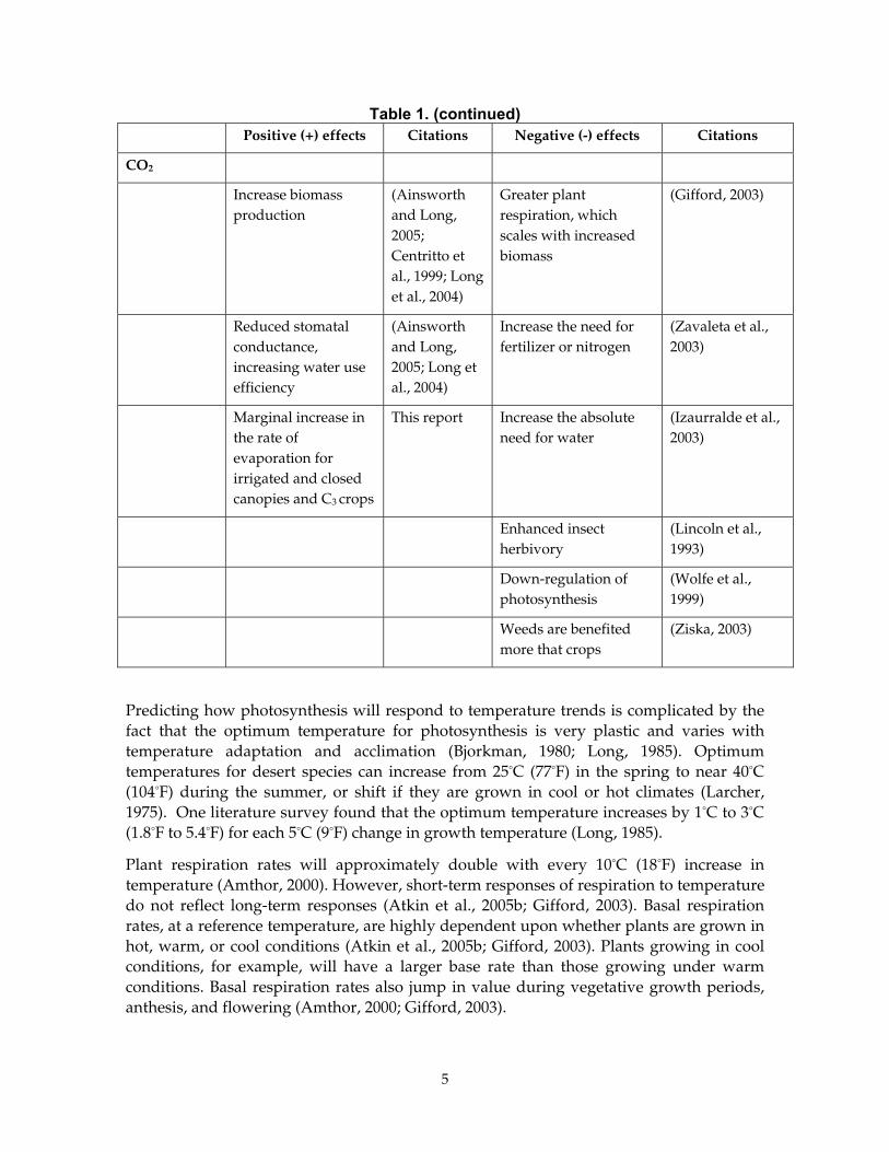
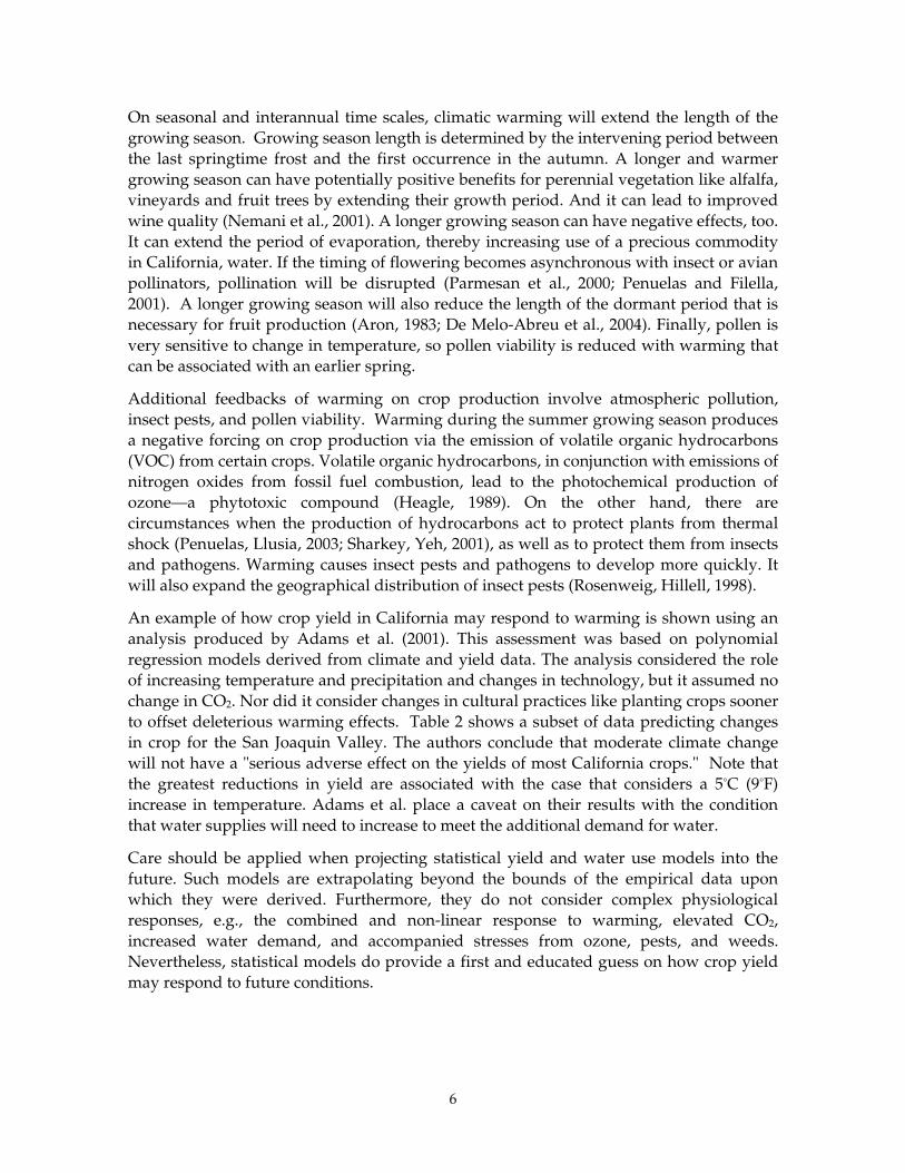
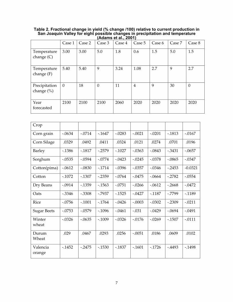
An example of how crop yield in California may respond to warming is shown using an analysis produced by Adams et al. (2001). This assessment was based on polynomial regression models derived from climate and yield data. The analysis considered the role of increasing temperature and precipitation and changes in technology, but it assumed no change in CO2. Nor did it consider changes in cultural practices like planting crops sooner to offset deleterious warming effects. Table 2 shows a subset of data predicting changes in crop for the San Joaquin Valley. The authors conclude that moderate climate change will not have a "serious adverse effect on the yields of most California crops." Note that the greatest reductions in yield are associated with the case that considers a 5°C (9°F) increase in temperature. Adams et al. place a caveat on their results with the condition that water supplies will need to increase to meet the additional demand for water.

Care should be applied when projecting statistical yield and water use models into the future. Such models are extrapolating beyond the bounds of the empirical data upon which they were derived. Furthermore, they do not consider complex physiological responses, e.g., the combined and non-linear response to warming, elevated CO2, increased water demand, and accompanied stresses from ozone, pests, and weeds. Nevertheless, statistical models do provide a first and educated guess on how crop yield may respond to future conditions.

7

Table 2. Fractional change in yield (% change /100) relative to current production in San Joaquin Valley for eight possible changes in precipitation and temperature

(Adams et al., 2001) Case 1 Case 2 Case 3 Case 4 Case 5 Case 6 Case 7 Case 8

Temperature change (C)

3.00

3.00 5.0 1.8 0.6 1.5 5.0 1.5

Temperature change (F)

5.40

5.40 9 3.24 1.08 2.7 9 2.7

Precipitation change (%)

0

18 0 11 4 9 30 0

Year forecasted

2100 2100 2100 2060 2020 2020 2020 2020

Crop

Corn grain -.0634 -.0714 -.1647 -.0283 -.0021 -.0201 -.1813 -.0167

Corn Silage .0329 .0492 .0411 .0324 .0121 .0274 .0701 .0196

Barley -.1386 -.1817 -.2579 -.1027 -.0363 -.0843 -.3431 -.0657

Sorghum -.0535 -.0594 -.0774 -.0423 -.0245 -.0378 -.0865 -.0347

Cotton(pima) -.0612 -.0830 -.1714 -.0396 -.0357 -.0346 -.2453 -0.0321

Cotton -.1072 -.1307 -.2359 -.0764 -.0475 -.0664 -.2782 -.0554

Dry Beans -.0914 -.1359 -.1563 -.0751 -.0266 -.0612 -.2668 -.0472

Oats -.3346 -.3308 -.7937 -.1525 -.0427 -.1187 -.7799 -.1189

Rice -.0756 -.1001 -.1764 -.0426 -.0003 -.0302 -.2309 -.0211

Sugar Beets -.0753 -.0579 -.1096 -.0461 -.031 -.0429 -.0694 -.0491

Winter wheat

-.0326 -.0635 -.1009 -.0326 -.0176 -.0269 -.1507 -.0111

Durum Wheat

.029 .0467 .0293 .0256 -.0051 .0186 .0609 .0102

Valencia orange

-.1452 -.2475 -.1530 -.1837 -.1601 -.1726 -.4493 -.1498

8

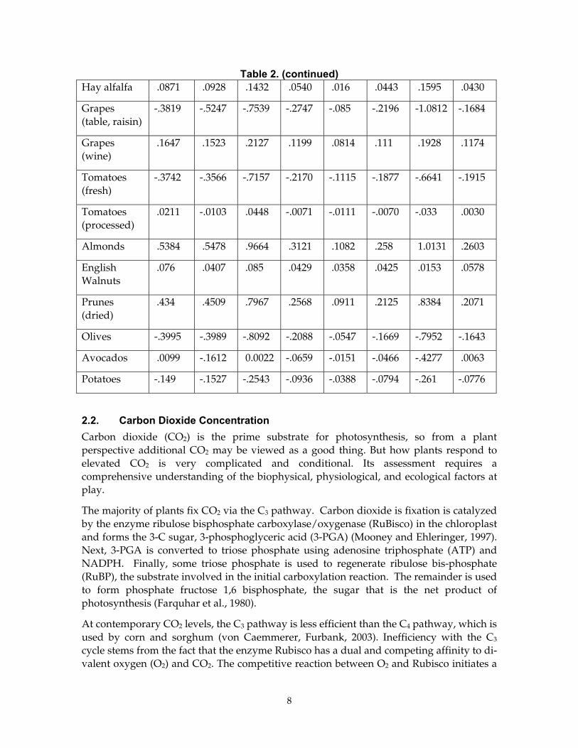
Table 2. (continued) Hay alfalfa .0871 .0928 .1432 .0540 .016 .0443 .1595 .0430

Grapes (table, raisin)

-.3819 -.5247 -.7539 -.2747 -.085 -.2196 -1.0812 -.1684

Grapes (wine)

.1647 .1523 .2127 .1199 .0814 .111 .1928 .1174

Tomatoes (fresh)

-.3742 -.3566 -.7157 -.2170 -.1115 -.1877 -.6641 -.1915

Tomatoes (processed)

.0211 -.0103 .0448 -.0071 -.0111 -.0070 -.033 .0030

Almonds .5384 .5478 .9664 .3121 .1082 .258 1.0131 .2603

English Walnuts

.076 .0407 .085 .0429 .0358 .0425 .0153 .0578

Prunes (dried)

.434 .4509 .7967 .2568 .0911 .2125 .8384 .2071

Olives -.3995 -.3989 -.8092 -.2088 -.0547 -.1669 -.7952 -.1643

Avocados .0099 -.1612 0.0022 -.0659 -.0151 -.0466 -.4277 .0063

Potatoes -.149 -.1527 -.2543 -.0936 -.0388 -.0794 -.261 -.0776

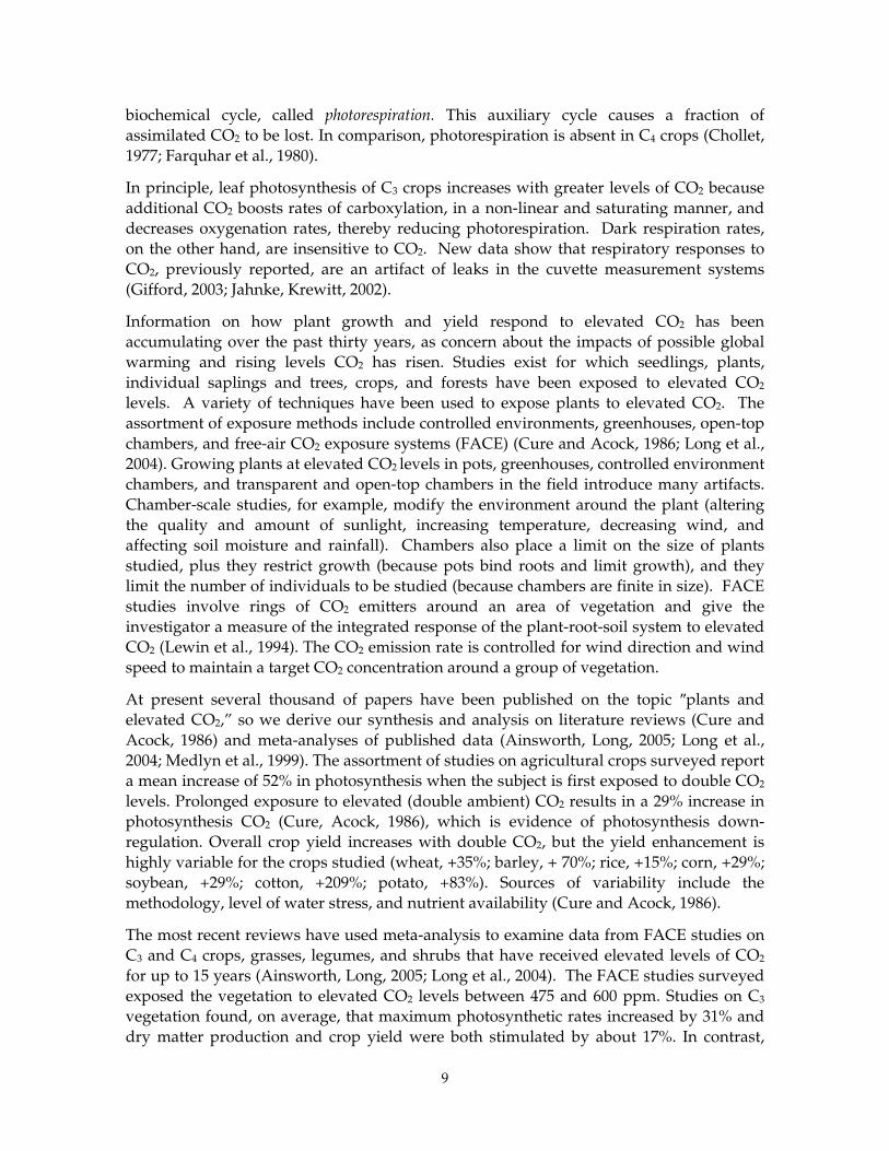
2.2. Carbon Dioxide Concentration Carbon dioxide (CO2) is the prime substrate for photosynthesis, so from a plant perspective additional CO2 may be viewed as a good thing. But how plants respond to elevated CO2 is very complicated and conditional. Its assessment requires a comprehensive understanding of the biophysical, physiological, and ecological factors at play.

The majority of plants fix CO2 via the C3 pathway. Carbon dioxide is fixation is catalyzed by the enzyme ribulose bisphosphate carboxylase/oxygenase (RuBisco) in the chloroplast and forms the 3-C sugar, 3-phosphoglyceric acid (3-PGA) (Mooney and Ehleringer, 1997). Next, 3-PGA is converted to triose phosphate using adenosine triphosphate (ATP) and NADPH. Finally, some triose phosphate is used to regenerate ribulose bis-phosphate (RuBP), the substrate involved in the initial carboxylation reaction. The remainder is used to form phosphate fructose 1,6 bisphosphate, the sugar that is the net product of photosynthesis (Farquhar et al., 1980).

At contemporary CO2 levels, the C3 pathway is less efficient than the C4 pathway, which is used by corn and sorghum (von Caemmerer, Furbank, 2003). Inefficiency with the C3 cycle stems from the fact that the enzyme Rubisco has a dual and competing affinity to di-valent oxygen (O2) and CO2. The competitive reaction between O2 and Rubisco initiates a

9

biochemical cycle, called photorespiration. This auxiliary cycle causes a fraction of assimilated CO2 to be lost. In comparison, photorespiration is absent in C4 crops (Chollet, 1977; Farquhar et al., 1980).

In principle, leaf photosynthesis of C3 crops increases with greater levels of CO2 because additional CO2 boosts rates of carboxylation, in a non-linear and saturating manner, and decreases oxygenation rates, thereby reducing photorespiration. Dark respiration rates, on the other hand, are insensitive to CO2. New data show that respiratory responses to CO2, previously reported, are an artifact of leaks in the cuvette measurement systems (Gifford, 2003; Jahnke, Krewitt, 2002).

Information on how plant growth and yield respond to elevated CO2 has been accumulating over the past thirty years, as concern about the impacts of possible global warming and rising levels CO2 has risen. Studies exist for which seedlings, plants, individual saplings and trees, crops, and forests have been exposed to elevated CO2 levels. A variety of techniques have been used to expose plants to elevated CO2. The assortment of exposure methods include controlled environments, greenhouses, open-top chambers, and free-air CO2 exposure systems (FACE) (Cure and Acock, 1986; Long et al., 2004). Growing plants at elevated CO2 levels in pots, greenhouses, controlled environment chambers, and transparent and open-top chambers in the field introduce many artifacts. Chamber-scale studies, for example, modify the environment around the plant (altering the quality and amount of sunlight, increasing temperature, decreasing wind, and affecting soil moisture and rainfall). Chambers also place a limit on the size of plants studied, plus they restrict growth (because pots bind roots and limit growth), and they limit the number of individuals to be studied (because chambers are finite in size). FACE studies involve rings of CO2 emitters around an area of vegetation and give the investigator a measure of the integrated response of the plant-root-soil system to elevated CO2 (Lewin et al., 1994). The CO2 emission rate is controlled for wind direction and wind speed to maintain a target CO2 concentration around a group of vegetation.

At present several thousand of papers have been published on the topic ″plants and elevated CO2,” so we derive our synthesis and analysis on literature reviews (Cure and Acock, 1986) and meta-analyses of published data (Ainsworth, Long, 2005; Long et al., 2004; Medlyn et al., 1999). The assortment of studies on agricultural crops surveyed report a mean increase of 52% in photosynthesis when the subject is first exposed to double CO2 levels. Prolonged exposure to elevated (double ambient) CO2 results in a 29% increase in photosynthesis CO2 (Cure, Acock, 1986), which is evidence of photosynthesis down-regulation. Overall crop yield increases with double CO2, but the yield enhancement is highly variable for the crops studied (wheat, +35%; barley, + 70%; rice, +15%; corn, +29%; soybean, +29%; cotton, +209%; potato, +83%). Sources of variability include the methodology, level of water stress, and nutrient availability (Cure and Acock, 1986).

The most recent reviews have used meta-analysis to examine data from FACE studies on C3 and C4 crops, grasses, legumes, and shrubs that have received elevated levels of CO2 for up to 15 years (Ainsworth, Long, 2005; Long et al., 2004). The FACE studies surveyed exposed the vegetation to elevated CO2 levels between 475 and 600 ppm. Studies on C3 vegetation found, on average, that maximum photosynthetic rates increased by 31% and dry matter production and crop yield were both stimulated by about 17%. In contrast,

10

stomatal conductance decreased by 20%, photosynthetic capacity (Vcmax) decreased by 13%, and specific leaf nitrogen mass decreased by 13%. Studies conducted on C4 vegetation found that elevated levels of CO2 increased photosynthesis by 15% to 20% and reduced stomatal conductance by 20%. The reduction in stomatal conductance was not significantly different from what was found for C3 vegetation.

Stomata partially close with elevated CO2 because a plant aims to maintain a balance between CO2 supply and demand. This is accomplished by keeping the ratio between internal and ambient CO2 near 0.7 for C3 plants and near 0.4 for C4 plants (Jones, 1992). The noted reduction in leaf nitrogen and Vcmax occurs in association with the down-regulation in photosynthesis (Wolfe et al., 1999). Sugars build up in a leaf because the demand for CO2 cannot keep up with supply. Sugars also activate genes, which in turn control the leaf’s nitrogen content and modulate its carboxylation velocity, Vcmax, a measure of photosynthetic capacity.

One explanation for greater vegetative growth at high CO2 levels is the “compound interest effect” (Centritto et al., 1999). Plants exposed to high CO2 get a faster initial jump on growth than those grown at ambient levels. However, the relative growth rate declines with time as a plant experiences a down-regulation in photosynthesis, self-shading and additional respiratory costs (Poorter, 1993). But nevertheless, the compound interest effect applied to the initial growth spurt leads to greater cumulative growth when plants are exposed to elevated CO2 (Centritto et al., 1999; Poorter, 1993). This is analogous to the fact that one will have more money in the bank when 4% interest is applied to an account with an initial deposit of $1000 than to one with an initial deposit of $500.

The meta-analyses and literature reviews surveyed do not examine the effect of elevated CO2 on whole plant respiration. However, we can deduce that respiration, at the canopy scale, will increase as crops become larger and their canopy photosynthesis rates increase. This will occur because plant respiration scales with photosynthesis and plant size (Gifford, 2003).

Exposure to both ozone and CO2 stimulates photosynthetic capacity relative to control conditions with normal CO2 and high ozone (Ainsworth and Long, 2005). This response is partly attributed to the fact that partial stomatal closure, associated with high CO2, reduces damage to plants exposed to elevated ozone levels.

11

3.0 Water Use At the regional and global scale, inferential evidence, based on measurements of continental river runoff and land surface climate models, suggests that growing levels of CO2 are reducing transpiration (Gedney et al., 2006). Yet, it is difficult to isolate and evaluate how evaporation may respond to elevated CO2 and temperature without introducing artifacts. We can, however, use theory and observations to deduce how evaporation from irrigated agricultural crops may change. In principle, partial stomatal closure (that is associated with elevated CO2 levels) decreases transpiration and increases water use efficiency (Cowan and Farquhar, 1977). However, feedback and feedforward effects, associated with the surface energy balance, occur and complicate the response of transpiration to elevated CO2 at the plant and field level (Farquhar et al., 1978; Mcnaughton and Jarvis, 1991). With no feedbacks between stomatal conductance, transpiration, and humidity, a linear decrease in stomatal conductance will produce a linear reduction in transpiration. But in nature, stomatal closure will induce an increase in leaf temperature. And because saturation vapor pressure is an exponential function of temperature, the humidity deficit between the leaf and atmosphere will be reinforced. Consequently partial stomatal closure promotes a feedback that modulates the direct effect of stomatal closure on transpiration.

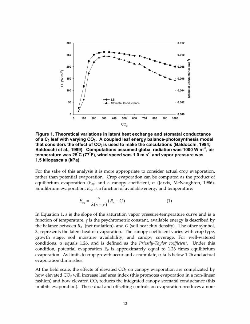
Model calculations of latent heat exchange for a sunlit leaf, based on a coupled leaf energy balance-photosynthesis model, demonstrate how leaf transpiration will vary with changes in CO2. In theory, increasing CO2 from 350 to 700 ppm will decrease stomatal conductance by 18%, but it will reduce transpiration by only 9% (Figure 1). If a down-regulation in photosynthesis occurs, the expected reduction in stomatal conductance and transpiration will be smaller.

How can we use this information to assess how evaporation will change in the future across the agriculture region of California? First we need to assess a baseline, the current amount of potential evaporation. Potential evaporation (E0) is defined as the evaporation rate from a well-watered, short, green surface. It is a metric that is commonly assessed from meteorological stations and is adjusted to reflect actual evaporation. Potential evaporation, based on data from a network of CIMIS stations in California, is on the order of 1344 +/- 70 mm per year over the period 1990 to 2001 (Hidalgo et al., 2005). Conceptually warming will reinforce additional potential evaporation. On the other hand, a restoring force on potential evaporation will be imposed by an increase in humidity, clouds and aerosols, factors that either decrease available sunlight (Roderick, Farquhar, 2002) or reduced the vapor pressure deficit of the atmosphere (Brutsaert, Parlange, 1998). At present no trends in potential evaporation have been detected across California (Hidalgo et al., 2005).

12

CO2

0 100 200 300 400 500 600 700 800 900 1000

LE (W

m-2 )

0

50

100

150

200

250

300

Stom

atal

Con

duct

ance

(ms-1

)

0.000

0.002

0.004

0.006

0.008

0.010

0.012

LEStomatal Conductance

Figure 1. Theoretical variations in latent heat exchange and stomatal conductance of a C3 leaf with varying CO2. A coupled leaf energy balance-photosynthesis model that considers the effect of CO2 is used to make the calculations (Baldocchi, 1994; Baldocchi et al., 1999). Computations assumed global radiation was 1000 W m-2, air temperature was 25°C (77°F), wind speed was 1.0 m s-1 and vapor pressure was 1.5 kilopascals (kPa).

For the sake of this analysis it is more appropriate to consider actual crop evaporation, rather than potential evaporation. Crop evaporation can be computed as the product of equilibrium evaporation (Eeq) and a canopy coefficient, α (Jarvis, McNaughton, 1986). Equilibrium evaporation, Eeq, is a function of available energy and temperature:

E ss

R Geq n=+

−λ γ( )

( ) (1)

In Equation 1, s is the slope of the saturation vapor pressure-temperature curve and is a function of temperature, γ is the psychrometric constant, available energy is described by the balance between Rn (net radiation), and G (soil heat flux density). The other symbol, λ, represents the latent heat of evaporation. The canopy coefficient varies with crop type, growth stage, soil moisture availability, and canopy coverage. For well-watered conditions, α equals 1.26, and is defined as the Priestly-Taylor coefficient. Under this condition, potential evaporation E0 is approximately equal to 1.26 times equilibrium evaporation. As limits to crop growth occur and accumulate, α falls below 1.26 and actual evaporation diminishes.

At the field scale, the effects of elevated CO2 on canopy evaporation are complicated by how elevated CO2 will increase leaf area index (this promotes evaporation in a non-linear fashion) and how elevated CO2 reduces the integrated canopy stomatal conductance (this inhibits evaporation). These dual and offsetting controls on evaporation produces a non-

13

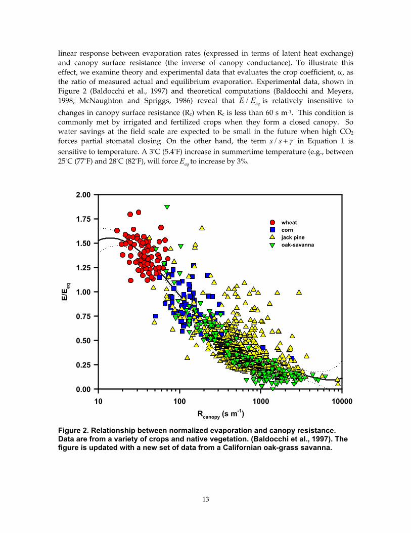
linear response between evaporation rates (expressed in terms of latent heat exchange) and canopy surface resistance (the inverse of canopy conductance). To illustrate this effect, we examine theory and experimental data that evaluates the crop coefficient, α, as the ratio of measured actual and equilibrium evaporation. Experimental data, shown in Figure 2 (Baldocchi et al., 1997) and theoretical computations (Baldocchi and Meyers, 1998; McNaughton and Spriggs, 1986) reveal that E Eeq/ is relatively insensitive to

changes in canopy surface resistance (Rc) when Rc is less than 60 s m-1. This condition is commonly met by irrigated and fertilized crops when they form a closed canopy. So water savings at the field scale are expected to be small in the future when high CO2 forces partial stomatal closing. On the other hand, the term s s/ + γ in Equation 1 is sensitive to temperature. A 3°C (5.4°F) increase in summertime temperature (e.g., between 25°C (77°F) and 28°C (82°F), will force Eeq to increase by 3%.

Rcanopy (s m-1)10 100 1000 10000

E/E eq

0.00

0.25

0.50

0.75

1.00

1.25

1.50

1.75

2.00

wheatcornjack pineoak-savanna

Figure 2. Relationship between normalized evaporation and canopy resistance. Data are from a variety of crops and native vegetation. (Baldocchi et al., 1997). The figure is updated with a new set of data from a Californian oak-grass savanna.

14

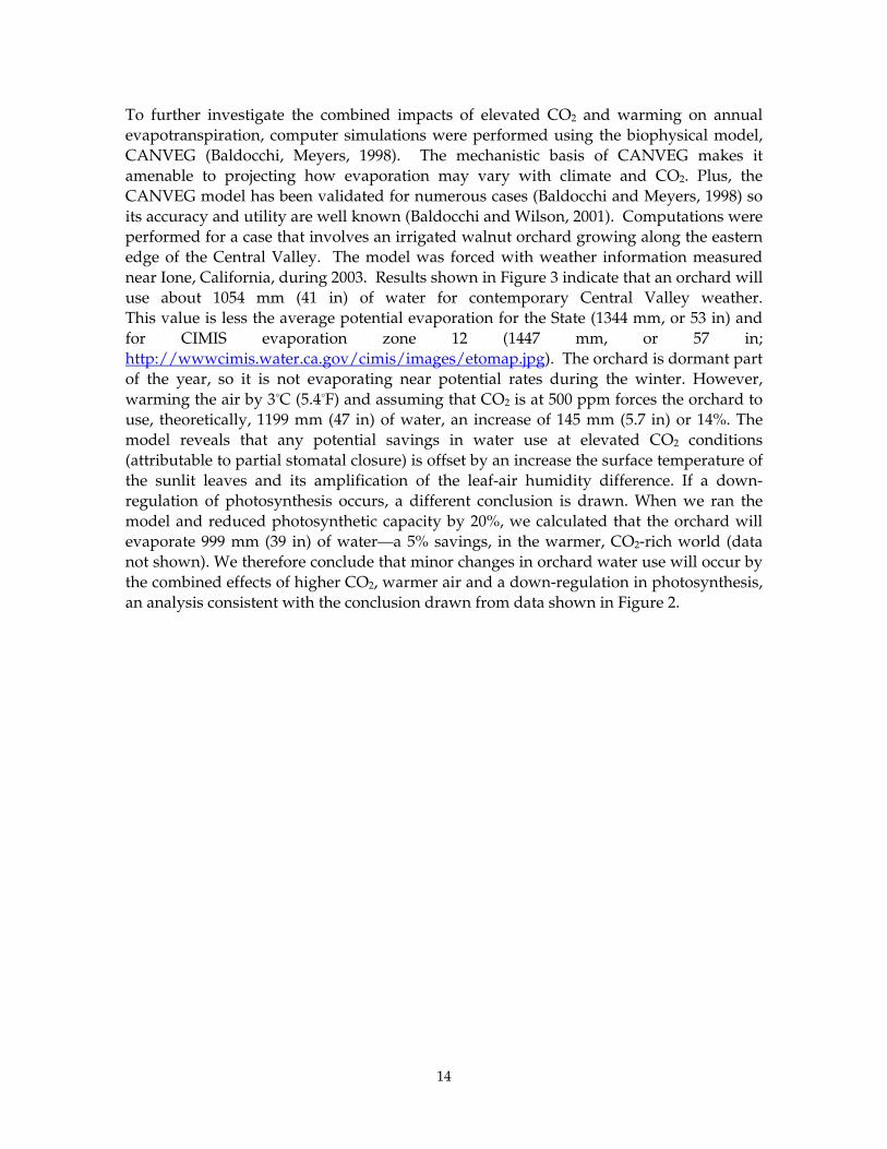
To further investigate the combined impacts of elevated CO2 and warming on annual evapotranspiration, computer simulations were performed using the biophysical model, CANVEG (Baldocchi, Meyers, 1998). The mechanistic basis of CANVEG makes it amenable to projecting how evaporation may vary with climate and CO2. Plus, the CANVEG model has been validated for numerous cases (Baldocchi and Meyers, 1998) so its accuracy and utility are well known (Baldocchi and Wilson, 2001). Computations were performed for a case that involves an irrigated walnut orchard growing along the eastern edge of the Central Valley. The model was forced with weather information measured near Ione, California, during 2003. Results shown in Figure 3 indicate that an orchard will use about 1054 mm (41 in) of water for contemporary Central Valley weather. This value is less the average potential evaporation for the State (1344 mm, or 53 in) and for CIMIS evaporation zone 12 (1447 mm, or 57 in; http://wwwcimis.water.ca.gov/cimis/images/etomap.jpg). The orchard is dormant part of the year, so it is not evaporating near potential rates during the winter. However, warming the air by 3°C (5.4°F) and assuming that CO2 is at 500 ppm forces the orchard to use, theoretically, 1199 mm (47 in) of water, an increase of 145 mm (5.7 in) or 14%. The model reveals that any potential savings in water use at elevated CO2 conditions (attributable to partial stomatal closure) is offset by an increase the surface temperature of the sunlit leaves and its amplification of the leaf-air humidity difference. If a down-regulation of photosynthesis occurs, a different conclusion is drawn. When we ran the model and reduced photosynthetic capacity by 20%, we calculated that the orchard will evaporate 999 mm (39 in) of water—a 5% savings, in the warmer, CO2-rich world (data not shown). We therefore conclude that minor changes in orchard water use will occur by the combined effects of higher CO2, warmer air and a down-regulation in photosynthesis, an analysis consistent with the conclusion drawn from data shown in Figure 2.

15

Walnuts2003 Climate data

Day

0 50 100 150 200 250 300 350 400

LE (W

m-2

)

0

50

100

150

200

250

ET: 1054 mm

Day

0 50 100 150 200 250 300 350 400

∆ LE

(W m

-2)

-20

0

20

40Ta + 3C, CO2 =500 ppmET: 1199 mm

Figure 3. Computation of evaporation from a California walnut orchard. Simulations are based on the CANVEG model. The top panel shows the seasonal course of daily average latent heat exchange for 2003 weather conditions. The bottom panel shows the difference in evaporation on the assumption that air

temperature increases 3°C and CO2 is at 500 ppm.

16

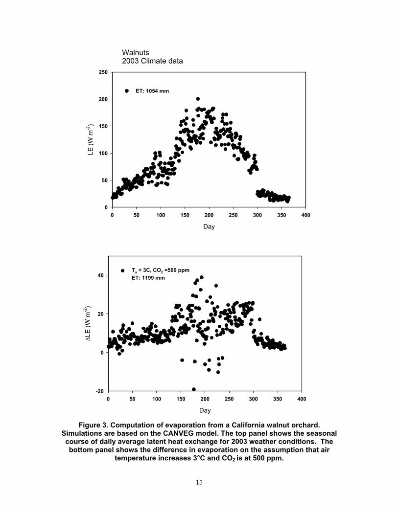
Simulations of regional water use produced by the general circulation climate model developed at the Hadley Centre in the United Kingdom indicates a small deduction (-7%) in evapotranspiration across the Pacific region, with an increase in CO2, to 560 ppm (Izaurralde et al., 2003) (Table 3). Combining warming scenarios and elevated CO2, on the other hand, produces an increase in regional evapotranspiration. Depending upon the degree of warming, evaporation can increase by 75 to 124 mm (3 to 5 in) per year. This response is consistent with computations based on the biophysical CANVEG model, despite the coarse-scale, the wetter climate scenario, and parameterized nature of the Hadley Centre evaporation sub-model (Hayhoe et al., 2004).

Table 3. Estimates of regional evaporation for the western Pacific region of the United States. Scenarios based on the Canadian Climate and Hadley Centre climate models are used. (Izaurralde et al., 2003)

Evaporation (mm)

Base: 365 ppm, 799 mm of precipitation, 12.2°C average air temperature

318

Change in evaporation

Base @ 560 ppm -7

H1 @ 560 ppm, + 44 mm of ppt, + 1°C in maximum temperature

75

H2 @ 560 ppm, +164 mm of precipitation, + 2.9°C maximum temperature

124

17

4.0 Contemporary Temperature Trends The previous agricultural-climate analysis by Hayhoe et al. (2004) focused primarily on trends in mean temperature. Here we examine other temperature statistics that are meaningful to agriculture and are buried within long-term climate data. Examples include summation of chilling temperature and probability statistics associated with exceeding critical temperatures.

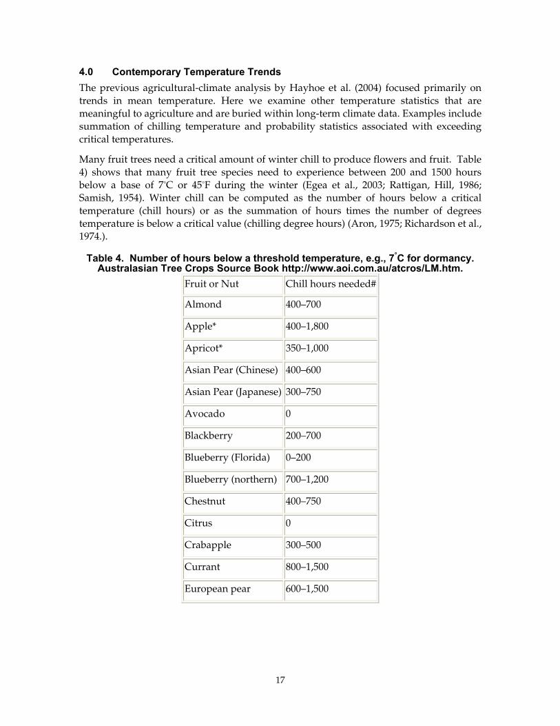
Many fruit trees need a critical amount of winter chill to produce flowers and fruit. Table 4) shows that many fruit tree species need to experience between 200 and 1500 hours below a base of 7°C or 45°F during the winter (Egea et al., 2003; Rattigan, Hill, 1986; Samish, 1954). Winter chill can be computed as the number of hours below a critical temperature (chill hours) or as the summation of hours times the number of degrees temperature is below a critical value (chilling degree hours) (Aron, 1975; Richardson et al., 1974.).

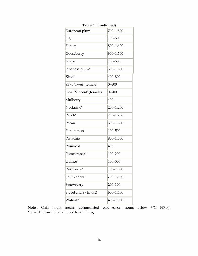
Table 4. Number of hours below a threshold temperature, e.g., 7°C for dormancy. Australasian Tree Crops Source Book http://www.aoi.com.au/atcros/LM.htm.

Fruit or Nut Chill hours needed#

Almond 400–700

Apple* 400–1,800

Apricot* 350–1,000

Asian Pear (Chinese) 400–600

Asian Pear (Japanese) 300–750

Avocado 0

Blackberry 200–700

Blueberry (Florida) 0–200

Blueberry (northern) 700–1,200

Chestnut 400–750

Citrus 0

Crabapple 300–500

Currant 800–1,500

European pear 600–1,500

18

Table 4. (continued) European plum 700–1,800

Fig 100–500

Filbert 800–1,600

Gooseberry 800–1,500

Grape 100–500

Japanese plum* 500–1,600

Kiwi* 400–800

Kiwi 'Twei' (female) 0–200

Kiwi 'Vincent' (female) 0–200

Mulberry 400

Nectarine* 200–1,200

Peach* 200–1,200

Pecan 300–1,600

Persimmon 100–500

Pistachio 800–1,000

Plum-cot 400

Pomegranate 100–200

Quince 100–500

Raspberry* 100–1,800

Sour cherry 700–1,300

Strawberry 200–300

Sweet cherry (most) 600–1,400

Walnut* 400–1,500

Note : Chill hours means accumulated cold-season hours below 7°C (45°F). *Low-chill varieties that need less chilling.

19

Under current climate conditions this dormancy is met because prolonged periods of fog in the Valley enable the trees to experience a sufficient period below a certain temperature threshold (e.g., 45°F, 7°C). In the event of climate warming we hypothesize that regional and global warming will reduce accumulated number of chill degree hours or chill hours in the fruit-growing region of California. In principle, a reduction in chill degree hours will result in a reduction in crop yield and quality. If true, this effect could have major economic and social consequences on fruit product in California. And if critical thresholds are reached with further warming (see Table 4), sustained production of high-value fruit crops like almonds, cherries, apricots, and others will be in jeopardy.

We based our analysis on a combination of CIMIS and National Weather Service (NWS) Coop climate data, available through the California Climate Archive.1 The CIMIS data is hourly, so it is ideal for computing accumulated winter chill hours, but unfortunately the data record is for a short duration to detect climate trends with confidence as it started in the 1980s. The NWS coop database, on the other hand, allows us to investigate longer climate trends, because many sites go back to the 1930s. However, this database only produces information on daily maximum and minimum temperature. To harmonize the databases, we first used the CIMIS dataset to develop and test an analytical equation for computing accumulated chill hours from maximum and minimum temperature measurements. Then we used the long coop data record to examine if there were trends in chill hours and to extend the spatial extent of the study.

Winter chill-degree hours (CDH) were summed between November 1 and Feb 28. On a daily basis the number of chill hours is computed relative to a reference temperature, in this case 45 oF.

CHD T T tref= −∑ ( )0

24 (2)

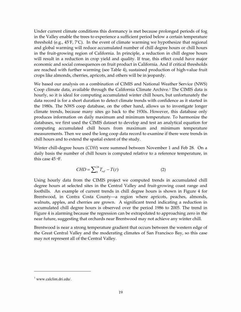
Using hourly data from the CIMIS project we computed trends in accumulated chill degree hours at selected sites in the Central Valley and fruit-growing coast range and foothills. An example of current trends in chill degree hours is shown in Figure 4 for Brentwood, in Contra Costa County—a region where apricots, peaches, almonds, walnuts, apples, and cherries are grown. A significant trend indicating a reduction in accumulated chill degree hours is observed over the period 1986 to 2005. The trend in Figure 4 is alarming because the regression can be extrapolated to approaching zero in the near future, suggesting that orchards near Brentwood may not achieve any winter chill.

Brentwood is near a strong temperature gradient that occurs between the western edge of the Great Central Valley and the moderating climates of San Francisco Bay, so this case may not represent all of the Central Valley.

1 www.calclim.dri.edu/.

20

Brentwood, CA

Year

1986 1988 1990 1992 1994 1996 1998 2000 2002 2004 2006

Chi

ll D

egre

e H

ours

, 45F

Nov

1 th

roug

h Fe

b 29

0

2000

4000

6000

8000

10000

12000

14000

16000

18000

Figure 4. Trend in accumulated chill degree hours at Brentwood, California, between 1986 and 2005. The slope indicates a reduction of 422 chill degree hours per year. The coefficient of variation indicates that 48% of the variance in chill degree hours is explained by time.

To extend the duration and spatial extent of the data record this study used climate data from the network of National Weather Service Coop stations, which measure maximum and minimum temperature. To compute cumulative chill degree hours from such data we applied trigonometric concepts to an ideal diurnal temperature course. First we assumed that the diurnal temperature course can be described by two adjoined triangles—one between the daily mean and the minimum temperature and the other between the daily mean and the maximum temperature (Figure 5).

21

Tmin

Tmax

Tref

a

d

b

cθ

TaveNoon

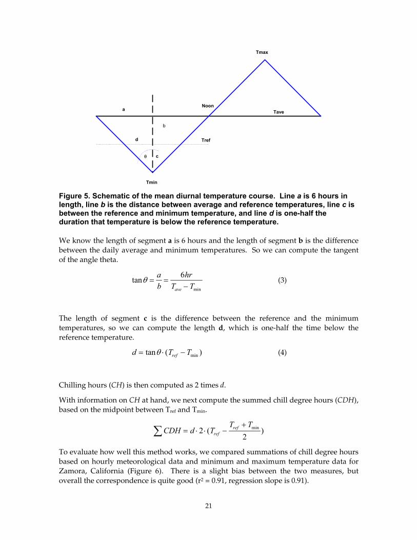
Figure 5. Schematic of the mean diurnal temperature course. Line a is 6 hours in length, line b is the distance between average and reference temperatures, line c is between the reference and minimum temperature, and line d is one-half the duration that temperature is below the reference temperature.

We know the length of segment a is 6 hours and the length of segment b is the difference between the daily average and minimum temperatures. So we can compute the tangent of the angle theta.

tanmin

θ = =−

ab

hrT Tave

6 (3)

The length of segment c is the difference between the reference and the minimum temperatures, so we can compute the length d, which is one-half the time below the reference temperature.

d T Tref= ⋅ −tan ( )minθ (4)

Chilling hours (CH) is then computed as 2 times d.

With information on CH at hand, we next compute the summed chill degree hours (CDH), based on the midpoint between Tref and Tmin.

CDH d TT T

refref∑ = ⋅ ⋅ −+

22

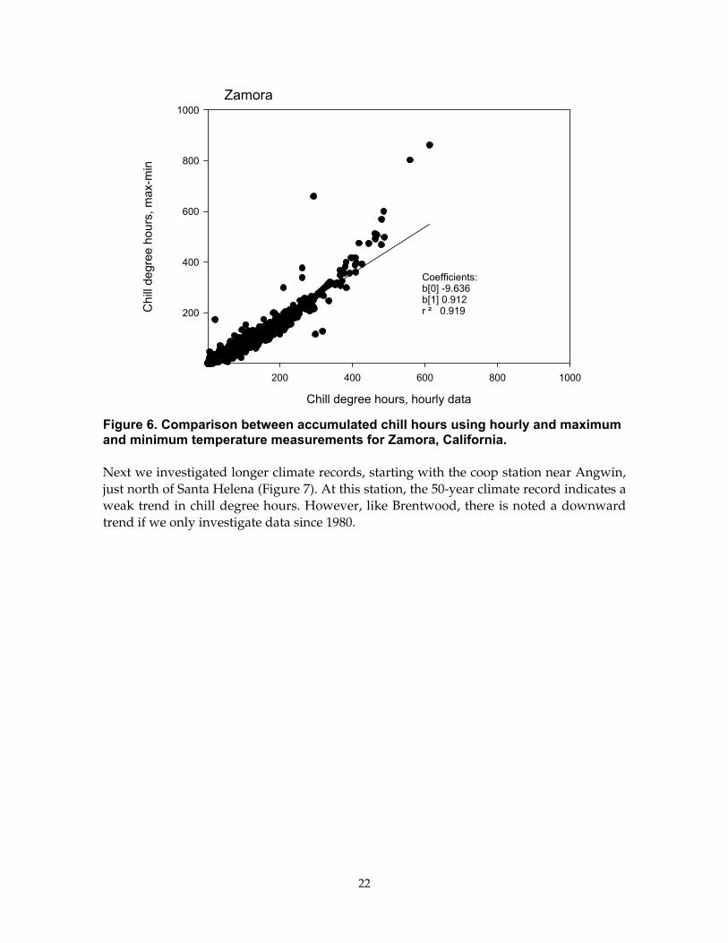
( )min

To evaluate how well this method works, we compared summations of chill degree hours based on hourly meteorological data and minimum and maximum temperature data for Zamora, California (Figure 6). There is a slight bias between the two measures, but overall the correspondence is quite good (r2 = 0.91, regression slope is 0.91).

22

Zamora

Chill degree hours, hourly data

200 400 600 800 1000

Chi

ll de

gree

hou

rs, m

ax-m

in

200

400

600

800

1000

Coefficients:b[0] -9.636b[1] 0.912r ² 0.919

Figure 6. Comparison between accumulated chill hours using hourly and maximum and minimum temperature measurements for Zamora, California.

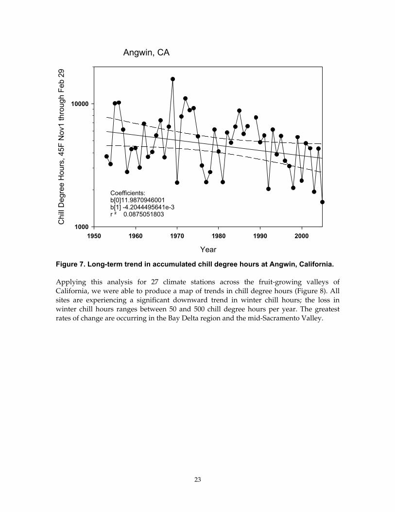
Next we investigated longer climate records, starting with the coop station near Angwin, just north of Santa Helena (Figure 7). At this station, the 50-year climate record indicates a weak trend in chill degree hours. However, like Brentwood, there is noted a downward trend if we only investigate data since 1980.

23

Angwin, CA

Year

1950 1960 1970 1980 1990 2000

Chi

ll D

egre

e H

ours

, 45F

Nov

1 th

roug

h Fe

b 29

1000

10000

Coefficients:b[0]11.9870946001b[1] -4.2044495641e-3r ² 0.0875051803

Figure 7. Long-term trend in accumulated chill degree hours at Angwin, California.

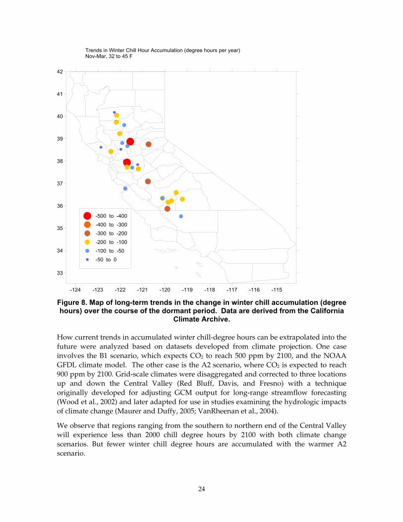
Applying this analysis for 27 climate stations across the fruit-growing valleys of California, we were able to produce a map of trends in chill degree hours (Figure 8). All sites are experiencing a significant downward trend in winter chill hours; the loss in winter chill hours ranges between 50 and 500 chill degree hours per year. The greatest rates of change are occurring in the Bay Delta region and the mid-Sacramento Valley.

24

-124 -123 -122 -121 -120 -119 -118 -117 -116 -115

33

34

35

36

37

38

39

40

41

42

-500 to -400 -400 to -300 -300 to -200 -200 to -100 -100 to -50 -50 to 0

Trends in Winter Chill Hour Accumulation (degree hours per year)Nov-Mar, 32 to 45 F

Figure 8. Map of long-term trends in the change in winter chill accumulation (degree hours) over the course of the dormant period. Data are derived from the California

Climate Archive.

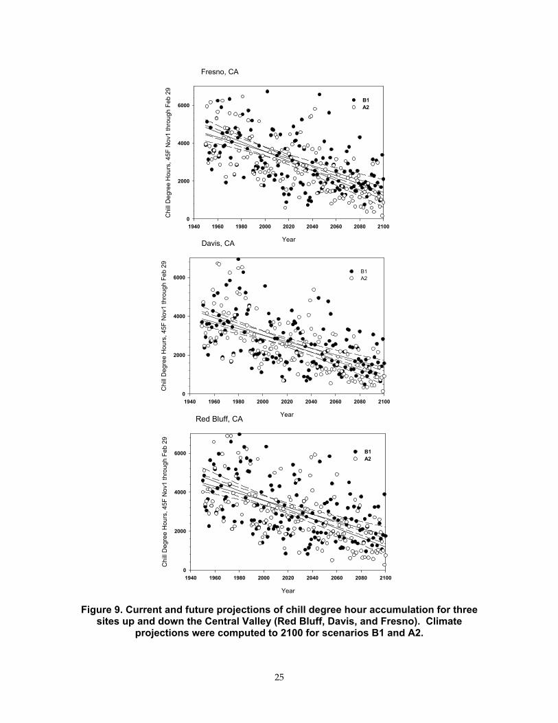
How current trends in accumulated winter chill-degree hours can be extrapolated into the future were analyzed based on datasets developed from climate projection. One case involves the B1 scenario, which expects CO2 to reach 500 ppm by 2100, and the NOAA GFDL climate model. The other case is the A2 scenario, where CO2 is expected to reach 900 ppm by 2100. Grid-scale climates were disaggregated and corrected to three locations up and down the Central Valley (Red Bluff, Davis, and Fresno) with a technique originally developed for adjusting GCM output for long-range streamflow forecasting (Wood et al., 2002) and later adapted for use in studies examining the hydrologic impacts of climate change (Maurer and Duffy, 2005; VanRheenan et al., 2004).

We observe that regions ranging from the southern to northern end of the Central Valley will experience less than 2000 chill degree hours by 2100 with both climate change scenarios. But fewer winter chill degree hours are accumulated with the warmer A2 scenario.

25

Red Bluff, CA

Year

1940 1960 1980 2000 2020 2040 2060 2080 2100

Chi

ll D

egre

e H

ours

, 45F

Nov

1 th

roug

h Fe

b 29

0

2000

4000

6000 B1A2

Davis, CA

Year

1940 1960 1980 2000 2020 2040 2060 2080 2100

Chi

ll D

egre

e H

ours

, 45F

Nov

1 th

roug

h Fe

b 29

0

2000

4000

6000B1A2

Fresno, CA

Year

1940 1960 1980 2000 2020 2040 2060 2080 2100

Chi

ll D

egre

e H

ours

, 45F

Nov

1 th

roug

h Fe

b 29

0

2000

4000

6000B1 A2

Figure 9. Current and future projections of chill degree hour accumulation for three sites up and down the Central Valley (Red Bluff, Davis, and Fresno). Climate

projections were computed to 2100 for scenarios B1 and A2.

26

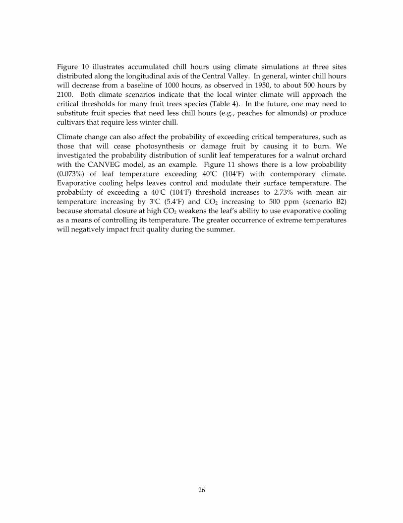
Figure 10 illustrates accumulated chill hours using climate simulations at three sites distributed along the longitudinal axis of the Central Valley. In general, winter chill hours will decrease from a baseline of 1000 hours, as observed in 1950, to about 500 hours by 2100. Both climate scenarios indicate that the local winter climate will approach the critical thresholds for many fruit trees species (Table 4). In the future, one may need to substitute fruit species that need less chill hours (e.g., peaches for almonds) or produce cultivars that require less winter chill.

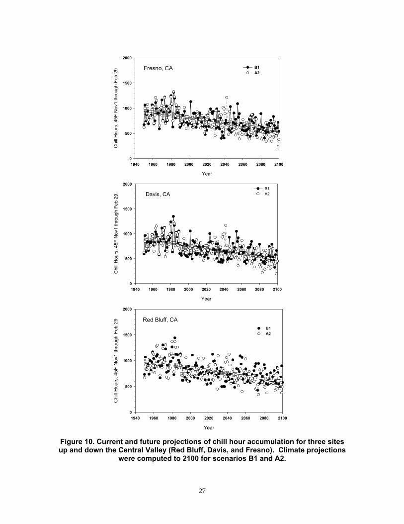
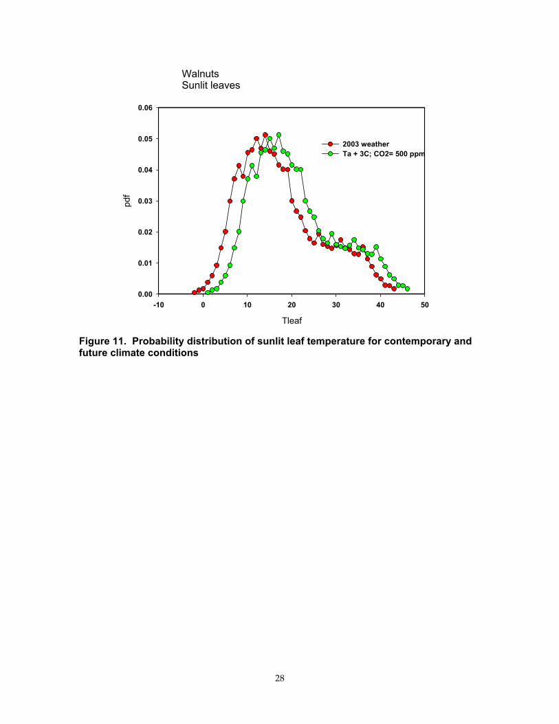
Climate change can also affect the probability of exceeding critical temperatures, such as those that will cease photosynthesis or damage fruit by causing it to burn. We investigated the probability distribution of sunlit leaf temperatures for a walnut orchard with the CANVEG model, as an example. Figure 11 shows there is a low probability (0.073%) of leaf temperature exceeding 40°C (104°F) with contemporary climate. Evaporative cooling helps leaves control and modulate their surface temperature. The probability of exceeding a 40°C (104°F) threshold increases to 2.73% with mean air temperature increasing by 3°C (5.4°F) and CO2 increasing to 500 ppm (scenario B2) because stomatal closure at high CO2 weakens the leaf’s ability to use evaporative cooling as a means of controlling its temperature. The greater occurrence of extreme temperatures will negatively impact fruit quality during the summer.

27

Fresno, CA

Year

1940 1960 1980 2000 2020 2040 2060 2080 2100

Chi

ll H

ours

, 45F

Nov

1 th

roug

h Fe

b 29

0

500

1000

1500

2000

B1 A2

Davis, CA

Year

1940 1960 1980 2000 2020 2040 2060 2080 2100

Chi

ll H

ours

, 45F

Nov

1 th

roug

h Fe

b 29

0

500

1000

1500

2000B1A2

Red Bluff, CA

Year

1940 1960 1980 2000 2020 2040 2060 2080 2100

Chi

ll H

ours

, 45F

Nov

1 th

roug

h Fe

b 29

0

500

1000

1500

2000

B1A2

Figure 10. Current and future projections of chill hour accumulation for three sites up and down the Central Valley (Red Bluff, Davis, and Fresno). Climate projections

were computed to 2100 for scenarios B1 and A2.

28

WalnutsSunlit leaves

Tleaf

-10 0 10 20 30 40 50

pdf

0.00

0.01

0.02

0.03

0.04

0.05

0.06

2003 weatherTa + 3C; CO2= 500 ppm

Figure 11. Probability distribution of sunlit leaf temperature for contemporary and future climate conditions

29

5.0 Conclusions This report has evaluated the effects of a warmer climate and high CO2 on aspects of California agriculture. Analysis was based on a survey of the scientific literature, application of biophysical models and an assessment of trends in current and future climate conditions.

This survey of the pertinent literature reveals a combination of positive and negative effects of warming and elevated CO2 on crop production. Elevated CO2 gives crops a spurt in growth, as photosynthesis responds positively to extra CO2. But enhanced photosynthesis is not sustained, as photosynthesis eventually experiences down-regulation. Indirect effects of elevated CO2 and warming on agriculture will include a lengthening of the growing and transpiration seasons, stimulation of weeds, and more insect pests. Pollination will be negatively impacted if warming causes asynchronization between flowering and the life cycle of insect pollinators.

Elevated CO2 causes stomata to close and have the potential to save water by reducing transpiration. But feedbacks between stomatal conductance, the temperature and humidity deficits of a leaf, and the air dampened the reduction in water savings. And indirect factors may increase water use because larger crops growing in a warmer climate will use more water, at the field scale. An assessment of water use for a walnut orchard for future conditions (temperature is 3°C (5.4°F) warmer and CO2 is 500 ppm) was conducted with a biophysical models. A typical orchard will use an additional 145 mm (5.7 in) of water in the future. Partial stomatal closure in a high-CO2 world increases leaf temperature of sunlit leaves and strengthens the vapor pressure gradient between leaves and the atmosphere.

Global warming may also affect fruit production in a negative manner. Fruit trees need 200 to 1200 hours of winter chill to flower. Long-term climate records, measured across the fruit-growing region of California, were scrutinized for trends in winter chilling degree-hours and chill hours. Global warming seems to be in motion, as all sites studied are experiencing a negative trend in winter chill accumulation. Calculations of trends in future chill, based on CO2 emission scenarios and use of a global change model, indicate that by 2100, the occurrence of adequate winter chill may be lost for many fruit species. The development of cultivars requiring less winter chill may be one way to circumvent this trend.

30

6.0 References Adams, R., J. Wu, L. L. Houston. (2001) The Effects of Climate Change on California Crops and Water Use, p. 182. California Energy Commision.

Ainsworth, E. A., and S. P. Long. (2005) "What have we learned from 15 years of free-air CO2 enrichment (FACE)? A meta-analytic review of the responses of photosynthesis, canopy properties and plant production to rising CO2." New Phytologist 165, 351-372.

Amthor, J. S. (1994) Higher plant respiration and its relationships to photosynthesis Springer Verlag, Berlin.

Amthor, J. S. (2000) "The McCree-de Wit-Penning de Vries-Thornley Respiration Paradigms: 30 Years Later." Annals of Botany 86, 1-20.

Aron, R. (1983) "Availability of chilling temperatures in California." Agricultural Meteorology 28, 351-363.

Aron, R. H. (1975) "A method for estimating the number of hours below a selected temperature threshold." Journal of Applied Meteorology 14, 1415-1418.

Atkin. O., D. Bruhn, V. Hurry, and M. Tjoelker. (2005a) "Evans Review No. 2: The hot and the cold: unravelling the variable response of plant respiration to temperature." Functional Plant Biology 32, 87-105.

Atkin, O. K., D. Bruhn, V. M. Hurry, M. G. Tjoelker. (2005b) "Evans Review No. 2: The hot and the cold: unravelling the variable response of plant respiration to temperature." Functional Plant Biology 32, 19.

Baldocchi, D. D. (1994) "An analytical solution for coupled leaf photosynthesis and stomatal conductance models." Tree Physiology 14, 1069-1079.

Baldocchi, D.D., J. Fuentes, D. Bowling, A. Turnipseed, R. Monson. (1999) "Scaling isoprene fluxes from leaves to canopies: test cases over a boreal aspen and a mixed temperate forest." Journal of Applied Meteorology 38, 885-898.

Baldocchi, D. D. and T. Meyers. (1998) "On using eco-physiological, micrometeorological and biogeochemical theory to evaluate carbon dioxide, water vapor and trace gas fluxes over vegetation: a perspective." Agricultural and Forest Meteorology 90, 1-25.

Baldocchi, D. D., C. A. Vogel, B. Hall. (1997) "Seasonal variation of energy and water vapor exchange rates above and below a boreal jackpine forest." Journal of Geophysical Research 102, 28939-28952.

Baldocchi, D. D., and K. B. Wilson.B (2001) "Modeling CO2 and water vapor exchange of a temperate broadleaved forest across hourly to decadal time scales." Ecological Modeling 142, 155-184.

Bjorkman, O. (1980) The response of photosynthesis to temperature. In: Plants and their atmospheric environment (eds. Grace J., E. D. Ford, and P. G. Jarvis), pp. 273-301. Blackwell, Oxford, UK.

31

Brutsaert, W., and M. B. Parlange. (1998) "Hydrologic cycle explains the evaporation paradox." Nature 396, 30.

California Agricultural Statistics Service. (2003) California Agriculture Overview, p. 10., Sacramento, California.

Cayan, D., S. Kammerdiener, M. Dettinger, J. Caprio, and D. Peterson. (2001) "Changes in the onset of spring in the western United States." Bulletin of the American Meteorological Society 82, 399-415.

Centritto, M., H. S. J. Lee, and P. G. Jarvis. (1999) "Increased growth in elevated [CO2]: An early, short-term response?" Global Change Biology 5, 623-633.

Chollet, R. (1977) "The biochemistry of photorespiration." Trends in Biochemical Sciences 2, 155-159.

Cowan I., and G. Farquhar. (1977) "Stomatal function in relation to leaf metabolism and environment." Symposium of the Society of Experimental Biology 31, 471-505.

Cure, J. D., and B. Acock. (1986) "Crop responses to carbon dioxide doubling: A literature survey." Agricultural and Forest Meteorology 38, 127-145.

De Melo-Abreu, J. P., D. Barranco, A. M. Cordeiro, et al. (2004) "Modelling olive flowering date using chilling for dormancy release and thermal time." Agricultural and Forest Meteorology 125, 117-127.

Easterling, D. R. (2002) "Recent changes in frost days and the frost free season in the United States." Bulletin of the American Meteorological Society.

Egea J., E. Ortega, P. Martinez-Gomez, and F. Dicenta. (2003) "Chilling and heat requirements of almond cultivars for flowering." Environmental and Experimental Botany 50, 79-85.

Farquhar, G. D., S. V. Caemmerer, and J. A. Berry. (1980) "A Biochemical-Model of Photosynthetic CO2 Assimilation in Leaves of C-3 Species." Planta 149, 78-90.

Farquhar, G. D., D. R. Dubbe, and K. Raschke. (1978) "Gain of Feedback Loop Involving Carbon-Dioxide and Stomata - Theory and Measurement." Plant Physiology 62, 406-412.

Feng, S., and Q. Hu. (2004) "Changes in agro-meteorological indicators in the contiguous United States: 1951-2000." Theoretical and Applied Climatology 78, 247-264.

Friedlingstein P., J-L. Dufresne, P. M. Cox, and P. Rayner. (2003) "How positive is the feedback between climate change and the carbon cycle?" Tellus B 55, 692-700.

Fung, I. Y., S. C. Doney, K. Lindsay, and J. John. (2005) "Evolution of carbon sinks in a changing climate." PNAS, 0504949102.

Gedney, N., P. M. Cox, R. A. Betts, et al. (2006) "Detection of a direct carbon dioxide effect in continental river runoff records." Nature 439, 835-838.

32

Gifford, R. (2003) "Plant respiration in productivity models: conceptualisation, representation and issues for global terrestrial carbon-cycle research." Functional Plant Biology 30, 171-186.

Harley, P., and J. Tenhunen. (1991) Modeling the photosynthetic response of C3 leaves to environmental factors. In: Modeling Crop Photosynthesis from Biochemistry to Canopy (eds. K. J. Boote, and R. S.Loomis), pp. 17-39. Crop Science Society of America, Madison, Wisc.

Hayhoe K., D. Cayan, C. Field, et al. (2004) Emissions pathways, climate change and impacts on California. Proceedings of the National Academy of Sciences of the United States of America 101, 12422-12427.

Heagle, A. S. (1989) Ozone and Crop Yield. Annual Review of Phytopathology 27, 397-423.

Hidalgo, H., D. Cayan, and M. Dettinger. (2005) "Sources of variability of evapotranspiration in California." Journal of Hydrometeorology 6, 3-19.

Izaurralde, R. C., N. J. Rosenberg, R. A. Brown, and A. M. Thomson. (2003) "Integrated assessment of Hadley Center (HadCM2) climate-change impacts on agricultural productivity and irrigation water supply in the conterminous United States: Part II. Regional agricultural production in 2030 and 2095." Agricultural and Forest Meteorology 117, 97-122.

Jahnke, S., and M. Krewitt. (2002) "Atmospheric CO2 concentration may directly affect leaf respiration measurement in tobacco, but not respiration itself." Plant, Cell and Environment 25, 641.

Jarvis, P. G., and K. G. McNaughton. (1986) "Stomatal Control of Transpiration - Scaling up from Leaf to Region." Advances in Ecological Research 15, 1-49.

Jones, H. G. (1992) Plants and microclimate: A quantitative approach to environmental plant physiology. Cambridge University Press, New York. p 51.

Larcher, W. (1975) Physiological Plant Ecology. Springer-Verlag, Berlin.

Lewin, K. F., G. R. Hendrey, J. Nagy, and R. L. LaMorte. (1994) "Design and application of a free-air carbon dioxide enrichment facility." Agricultural and Forest Meteorology 70, 15-29.

Lincoln, D. E., E. D. Fajer, and R. H. Johnson. (1993) "Plant-insect herbivore interactions in elevated CO2 environments." Trends in Ecology & Evolution 8, 64-68.

Long, S. P. (1985) Leaf gas exchange. In: Photosynthetic mechanisms and the environment (eds. Barber J, and N. R. Baker), 453-499. Elsevier Science Publisher.

Long, S. P., E. A. Ainsworth, A. Rogers, D. R. Ort. (2004) "RISING ATMOSPHERIC CARBON DIOXIDE: Plants FACE the Future.” Annual Review of Plant Biology 55, 591-628.

Manabe S., and R. Wetherald. (1975) "Effects of doubling CO2 concentration on climate of a general circulation model." Journal of Atmospheric Science 32, 3-15.

33

Maurer, E. P., and P. B. Duffy. (2005) "Uncertainty in Projections of Streamflow Changes due to Climate Change in California." Geophysical Research Letters 32, L03704 doi:10.1029/2004GL021462.

Mcnaughton, K. G., and P. G. Jarvis. (1991) "Effects of Spatial Scale on Stomatal Control of Transpiration." Agricultural and Forest Meteorology 54, 279-302.

McNaughton, K. G., and T. W. Spriggs. (1986) "A Mixed-Layer Model for Regional Evaporation." Boundary-Layer Meteorology 34, 243-262.

Medlyn, B. E., F-W. Badeck, D. G. G. De Pury, et al. (1999) "Effects of elevated CO2 on photosynthesis in European forest species: A meta-analysis of model parameters." Plant Cell Environ 22, 1475-1495.

Mooney, H. A., and J. R. Ehleringer. (1997) Photosynthesis. In: Plant Ecology (ed. Crawley M. J.), 1-27. Blackwell, Oxford.

Nemani, R. R., M. A. White, D. R. Cayan, et al. (2001) "Asymmetric warming over coastal California and its impact on the premium wine industry." Climate Research 19, 25-34.

Parmesan, C., T. Root, and M. Willig. (2000) "Impacts of extreme weather and climate on terrestrial biota." Bulletin of the American Meteorological Society 81, 443-450.

Penuelas, J., and I. Filella. (2001) "Phenology: Responses to a Warming World." Science 294, 793-795.

Penuelas, J., and J. Llusia. (2003) "BVOCs: Plant defense against climate warming?" Trends in Plant Science 8, 105-109.

Poorter, H. (1993) "Interspecific variation in the growth response of plants to an elevated ambient CO2 concentration." Plant Ecology (Historical Archive) 104-105, 77-97.

Prentice, I. C., M. Heimann, and S. Sitch. (2000) "The carbon balance of the terrestrial biosphere: Ecosystem models and atmospheric observations." Ecological Applications 10, 1553-1573.

Rattigan, K., and S. J. Hill. (1986) "Relationship between temperature and flowering in almond." Australian Journal of Experimental Agriculture 26, 399-404.

Richardson, E. A., S. D. Seeley, and D. R. Walker. (1974.) "A model for estimating the completion of rest for 'Redhaven' and 'Elberta' peach trees." HortScience 9, 331-332.

Roderick, M. L., and G. D. Farquhar. (2002) The Cause of Decreased Pan Evaporation over the Past 50 Years. Science 298, 1410-1411.

Rosenberg, N. J., R. A. Brown, R. C. Izaurralde, and A. M. Thomson. (2003) "Integrated assessment of Hadley Centre (HadCM2) climate change projections on agricultural productivity and irrigation water supply in the conterminous United States: I. Climate change scenarios and impacts on irrigation water supply simulated with the HUMUS model." Agricultural and Forest Meteorology 117, 73-96.

34

Rosenweig, C., and D. Hillell. (1998) Climate Change and the Global Harvest Oxford, Oxford, UK.

Samish, R. M. (1954) "Dormancy in Woody Plants." Annual Review of Plant Physiology 5, 183-204.

Sharkey, T. D., and S. Yeh. (2001) "Isoprene emission from plants." Annual Review of Plant Physiology and Plant Molecular Biology 52, 407-436.

Snyder, M. A , J. A. Bell, L. Sloan, P. B. Duffy, and B. Govindasamy. (2002) "Climate responses to a doubling of atmospheric carbon dioxide for a climatically vulnerable region." Geophysical Research Letters 29, 10.1029/2001GL014431.

Suckling, P. W., and M. D. Mitchell. (1988) "Fog Climatology of the Sacramento Urban Area." The Professional Geographer 40, 186-194.

Underwood, S. J., G. P. Ellrod, and A. L. Kuhnert. (2004) "A Multiple-Case Analysis of Nocturnal Radiation-Fog Development in the Central Valley of California Utilizing the GOES Nighttime Fog Product." Journal of Applied Meteorology 43, 297-311.

VanRheenan, N. T., A. W. Wood, R. N. Palmer, and D. P. Lettenmaier. (2004) "Potential implications of PCM climate change scenarios for Sacramento-San Joaquin River basin hydrology and water resources." Climatic Change 62, 257-281.

von Caemmerer, S., and R. Furbank. (2003) "The C4 pathway: An efficient CO2 pump." Photosynthesis Research 77, 191-207.

Wolfe, D. W., R. Gifford, D. Hilbert, Y. Luo. (1999) "Integration of photosynthetic acclimation to CO2 at the whole-plant level." Global Change Biology.

Wood, A. W., E. P. Maurer, A. Kumar, and D. P. Lettenmaier. (2002) "Long range experimental hydrologic forecasting for the eastern U.S." Journal of Geophysical Research 107, 4429.

Zavaleta, E. S., M. R. Shaw, N. R. Chiariello, H. A. Mooney, and C. B. Field. (2003) "Additive effects of simulated climate changes, elevated CO2, and nitrogen deposition on grassland diversity." PNAS 100, 7650-7654.

Ziska, L. (2003) "Evaluation of growth response of six invasive species to past, present, and future atmospheric CO." Journal of Experimental Botany 54, 395-406.