Embed Size (px)
Citation preview
POLITECNICO DI MILANO
Scuola di Ingegneria Industriale e dell'Informazione
Corso di Laurea Magistrale in
Ingegneria Gestionale
An assessment of the advantages of using TOC pull
replenishment in real situations
Supervisor: Miragliotta Giovanni
Co-supervisor: Buora Carlo
Master Graduate Thesis by:
Masdea Marco ID: 820364
Academic Year 2015 - 2016

i
Index of Contents
INDEX OF FIGURES ................................................................................III
INDEX OF TABLES ..................................................................................III
INDEX OF GRAPHS ................................................................................. IV
ABSTRACT ................................................................................................. V
1. INTRODUCTION 1
1.1 - COLLECTION AND REVIEW CRITERIA ..............................................................2
1.2 - GAPS ENCOUNTERED .....................................................................................8
1.3 - RESEARCH QUESTIONS ................................................................................ 10
2. TAXONOMY OF REPLENISHMENT STRATEGIES 11
2.1.1 - Push and Pull ................................................................................... 11
2.1.2 - Statistical Inventory Replenishment .................................................. 13 2.1.3 - Time-Phased Techniques: MRP and DRP ........................................ 19
2.1.4 - Lean Philosophy in Distribution ....................................................... 22
3. TOC PRINCIPLES AND PARADIGMS 25
3.1 - TOC GLOSSARY .......................................................................................... 27
3.1.1 - Constraints....................................................................................... 27
3.1.2 - Buffers ............................................................................................. 27
3.2 - LOGISTICS PARADIGM .................................................................................. 29
3.2.1 - Five Focusing Steps ......................................................................... 29 3.2.2 - VAT Analysis .................................................................................... 30
3.2.3 - Drum-Buffer-Rope ........................................................................... 31 3.2.4 - Buffer Management .......................................................................... 33
3.3 - PERFORMANCE MEASUREMENT ................................................................... 35
3.3.1 - Throughput Accounting .................................................................... 35
3.4 - DECISION MAKING ...................................................................................... 38
3.4.1 - Thinking Processes .......................................................................... 38
3.5 - TOC IN PRODUCTION ................................................................................... 40
3.5.1 - Simplified DBR ................................................................................ 40 3.5.2 - Make-To-Availability ....................................................................... 43
4. TOC AND SUPPLY CHAIN MANAGEMENT 47
4.1 - SUPPLY CHAIN REPLENISHMENT SYSTEM ..................................................... 47
4.1.1 - Aggregate Stock ............................................................................... 48 4.1.2 - Determine Buffer .............................................................................. 48
4.1.3 - Increase Replenishment Frequency .................................................. 50 4.1.4 - Manage Flow ................................................................................... 51
4.1.5 - Dynamic Buffer Management ........................................................... 52 4.1.6 - Set Manufacturing Priorities ............................................................ 55
4.2 - LOCAL PERFORMANCE MEASUREMENT ........................................................ 55
ii
5. SIMULATIONS OF REPLENISHMENT 57
5.1 - FEATURES OF THE MODEL ............................................................................57
5.1.1 - Structure of Network ........................................................................57 5.1.2 - Assumptions and Variables ..............................................................58
5.1.3 - Recorded Parameters .......................................................................61 5.1.4 - Formulas of Performances ...............................................................62
5.2 - MODELLED POLICIES ...................................................................................63
5.3 - SIMULATIONS ..............................................................................................65
5.3.1 - Scenario 1: Stationary demand with low variability..........................66 5.3.2 - Scenario 2: Stationary demand with higher variability .....................71
5.3.3 - Scenario 3: Demand with seasonality ...............................................81
6. CONCLUSIONS 85
6.1 - FINDINGS.....................................................................................................85
6.2 - LIMITS OF THE MODEL ..................................................................................89
6.3 - FURTHER DEVELOPMENTS ...........................................................................89
REFERENCES ........................................................................................... 90

iii
Index of Figures
Fig. 1: Growth of literature on TOC ...................................................................................... 4
Fig. 2: DRP in a multi-echelon supply chain ........................................................................ 20 Fig. 3: Five Lean Principles ................................................................................................. 22
Fig. 4: TOC Elements .......................................................................................................... 25 Fig. 5: Current state of TOC ................................................................................................ 26
Fig. 6: Types of buffer (adapted from Schragenheim & Dettmer, 2001) ................................ 28 Fig. 7: Five Focusing Steps cycle ......................................................................................... 29
Fig. 8: Network Typologies in VATI Analysis ....................................................................... 30 Fig. 9: Traditional DBR (adapted from Schragenheim & Dettmer, 2001) ............................. 32
Fig. 10: Buffer Zonation ...................................................................................................... 33 Fig. 11: Planned Load ......................................................................................................... 41
Fig. 12: Estimation of Safe Due Dates ................................................................................. 42 Fig. 13: Buffer Status ........................................................................................................... 51
Fig. 14: Dynamic Buffer Management ................................................................................. 53 Fig. 15: Network Model ....................................................................................................... 57
Index of Tables
Table 1: Papers and Articles selected..................................................................................... 3
Table 2: Categorization of Papers.......................................................................................... 5 Table 3: TOC Branches researched ....................................................................................... 5
Table 4: Basic Replenishment Strategies .............................................................................. 14 Table 5: Ordering Policy (adapted from Wensing, 2011) ..................................................... 16
Table 6: Networks configurations in VAT Analysis (adapted from Lockamy, 2008) .............. 31 Table 7: Common TOC Performance metrics ....................................................................... 37
Table 8: Example of Throughput Accounting (adapted from Cox & Schleier, 2010) ............. 37 Table 9: Local Performance Measures ................................................................................. 55
Table 10: Recorded Parameters ........................................................................................... 62 Table 11: Formulas.............................................................................................................. 62
Table 12: ROP, low variability............................................................................................. 66 Table 13: ROP, low var., minimum saturation and priority to profit..................................... 67
Table 14: DBM, low variability ............................................................................................ 68 Table 15: ROP, higher variability ........................................................................................ 71
Table 16: ROP, higher var., minimum saturation and priority to profit ................................ 72 Table 17: DBM Variations - Target resize and Cooling time ................................................ 73
Table 18: DBM Variations - Enhancement to Trigger of TMR.............................................. 76 Table 19: DBM vs ROP - Target Resize 10% and Trigger TMR 90% ................................... 78
Table 20: DBM - Order Batching ......................................................................................... 79 Table 21: DBM with batch ................................................................................................... 80 Table 22: ROP, seasonality .................................................................................................. 81
Table 23: DBM Variations: Target Resize and Trigger TMR with seasonality ...................... 82
iv
Index of Graphs
Graph 1: Scenario 1 - ROP, low variability.......................................................................... 66
Graph 2: Scenario 1 - Loading Priority to Profitability ........................................................ 67 Graph 3: Scenario 1 - DBM vs ROP, low variability ............................................................ 68
Graph 4: Scenario 2 - ROP, higher variability ..................................................................... 71 Graph 5: Scenario 2 - Loading Priority to Profitability ........................................................ 72
Graph 6: Scenario 2 - DBM Variations: Target resize and Cooling time .............................. 74 Graph 7: Scenario 2 - DBM Variations: enhancement to Trigger of TMR ............................ 77
Graph 8: Scenario 2 - DBM vs ROP: Target resize 10% and Trigger TMR 90% .................. 78 Graph 9: Scenario 2 - DBM with batch ................................................................................ 79
Graph 10: Scenario 2 - DBM with batch vs ROP.................................................................. 80 Graph 11: Scenario 3 - ROP, seasonality ............................................................................. 81
Graph 12: Scenario 3 - DBM Variations: Target resize and Cooling time with seasonality .. 83 Graph 13: Scenario 3 - DBM vs ROP, seasonality ............................................................... 84
v
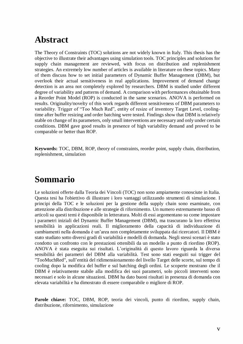
Abstract
The Theory of Constraints (TOC) solutions are not widely known in Italy. This thesis has the
objective to illustrate their advantages using simulation tools. TOC principles and solutions for
supply chain management are reviewed, with focus on distribution and replenishment
strategies. An extremely low number of articles is available in literature on these topics. Many
of them discuss how to set initial parameters of Dynamic Buffer Management (DBM), but
overlook their actual sensitiveness in real applications. Improvement of demand change
detection is an area not completely explored by researchers. DBM is studied under different
degree of variability and patterns of demand. A comparison with performances obtainable from
a Reorder Point Model (ROP) is conducted in the same scenarios. ANOVA is performed on
results. Originality/novelty of this work regards different sensitiveness of DBM parameters to
variability. Trigger of “Too Much Red”, entity of resize of inventory Target Level, cooling-
time after buffer resizing and order batching were tested. Findings show that DBM is relatively
stable on change of its parameters, only small interventions are necessary and only under certain
conditions. DBM gave good results in presence of high variability demand and proved to be
comparable or better than ROP.
Keywords: TOC, DBM, ROP, theory of constraints, reorder point, supply chain, distribution,
replenishment, simulation
Sommario
Le soluzioni offerte dalla Teoria dei Vincoli (TOC) non sono ampiamente conosciute in Italia.
Questa tesi ha l'obiettivo di illustrare i loro vantaggi utilizzando strumenti di simulazione. I
principi della TOC e le soluzioni per la gestione della supply chain sono esaminate, con
attenzione alla distribuzione e alle strategie di rifornimento. Un numero estremamente basso di
articoli su questi temi è disponibile in letteratura. Molti di essi argomentano su come impostare
i parametri iniziali del Dynamic Buffer Management (DBM), ma trascurano la loro effettiva
sensibilità in applicazioni reali. Il miglioramento della capacità di individuazione di
cambiamenti nella domanda è un’area non completamente sviluppata dai ricercatori. Il DBM è
stato studiato sotto diversi gradi di variabilità e modelli di domanda. Negli stessi scenari è stato
condotto un confronto con le prestazioni ottenibili da un modello a punto di riordino (ROP).
ANOVA è stata eseguita sui risultati. L’originalità di questo lavoro riguarda la diversa
sensibilità dei parametri del DBM alla variabilità. Test sono stati eseguiti sui trigger del
"TooMuchRed", sull’entità del ridimensionamento del livello Target delle scorte, sul tempo di
cooling dopo la modifica del buffer e sul batching degli ordini. Le scoperte mostrano che il
DBM è relativamente stabile alla modifica dei suoi parametri, solo piccoli interventi sono
necessari e solo in alcune situazioni. DBM ha dato buoni risultati in presenza di domanda con
elevata variabilità e ha dimostrato di essere comparabile o migliore di ROP.
Parole chiave: TOC, DBM, ROP, teoria dei vincoli, punto di riordino, supply chain,
distribuzione, rifornimento, simulazione

vi
1
1. Introduction
Distribution has always been critical for many industries. Availability is considered a given by
customers and today stockouts have a greater impact on reputation and customer retention than
in the past. At the same time, distribution networks have grown larger and more complex than
ever. Challenging goals like minimization of total costs and improvement of service level are
even more tough in this context. In distribution networks, transportation costs are high,
especially if they are world-wide extended. Due dates are extremely important in supply chains
and firms are often on the verge of delays, which are paid with relevant penalties.
An effective planning and replenishment strategies are vital in order to simplify these
complexities.
The aim of this thesis is to evaluate Theory of Constraints (TOC) pull replenishment strategies
and describe their advantages in real situations using simulation tools. Distribution and
replenishment management literature is constantly developing. In spite of it, this theory is not
really well known in Italy.
In order to provide the whole picture, three preliminary steps were made:
1) Determine the basis of TOC and its state of development.
2) Determine a framework of the major replenishment strategies.
3) Determine the rules of TOC Pull Replenishment for distribution.
Gaps encountered have generated some research questions. Simulation scenarios were
modelled to answer them and they were tested using the tools of Rockwell ARENA. Results
were collected in MS EXCEL for a preliminary study, while statistical analysis and ANOVA
were conducted using software ERRE.
Originality of this work regards different sensitiveness of DBM parameters to variability that
they could face in real applications of TOC replenishment solutions. DBM has many parameters
but their effects are not clearly assessed in relation to variability of demand. Possible corrections
operated by controllers will be simulated and compared.

1. Introduction
2
1.1 - Collection and Review Criteria
Literature review was conducted by following a structured and systematic approach as
suggested by (Tranfield et al., 2003). This methodology has been employed by many researches
on logistics and supply chain management; the following three-steps are a variation of those
adopted by (Mangiaracina et al., 2015).
STEP 1 - ARTICLES SELECTION
Classification context: Literature evaluated in this work is about replenishment strategies in
downstream of supply chains. Different levels of integration between distribution and
production was taken into consideration, although the focus of this thesis is only on
distribution topics. Focus is on Theory of Constraints and its related methodologies.
Definition of the unit of analysis: The main sources of the collected information were
journals and articles, considering only those peer reviewed. Conference proceedings were
not included. Citations from books and manuals of high impact were added to provide a
more solid basis to the assertions of this work and to complete information scarcity on some
topics.
Collecting publications: Articles were selected from databases like Scopus and Web of
Science or downloaded from sites of publishers Springer Link, Science Direct (Elsevier),
Wiley Online, Emerald Insight, JSTOR and other. The main journals articles come from
are:
- Journal of Operations Management (JOM)
- European Journal of Operational Research (EJOR)
- Production and Operations Management (POM)
- Manufacturing and Service Operations Management (MSOM)
- International Journal of Production Research (IJPR)
- International Journal of Production Economics (IJPE)
- International Journal of Operations and Production Management (IJOPM)
The keywords entered to filter databases were combinations of the following words:
“Supply chain”, “Theory of Constraints”, “Replenishment”, “Dynamic Buffer
Management”, “Simulation”, “Distribution”, “Inventory Management”, “Policy”. Thanks
to these filtering criteria, their presence in title and abstract have been analysed, limiting the

1. Introduction
3
search to Business, Management and Economics fields and Decision Science or those
related to Engineering.
Delimiting Fields: Documents including the words “Theory of Constraints” in title, abstract
or keywords were 1082 (searched in Scopus, August 2016), without distinction about area,
document type, specific topic or temporal restriction of sources. Some of them were written
even before 1980 and some other were not related with TOC; after their removal a total of
954 was selected. Filtering only articles and reviews from journals they were reduced to
556.
A search by keywords connected with supply chain management sorted 146 papers. A
refinement was conducted by reading titles and abstracts and selecting appropriate subject
areas, as Management and Decision Science. Ignoring those dedicated exclusively to
production or matters not directly linked to distribution, no more than 74 articles were
reputed of direct interest. Finally, those not dealing with topics of distribution,
replenishment or inventory control were excluded.
The selection highlighted 23 articles related to the topics of this thesis. Because of their
little amount, a new search was conducted on other databases (like Web of Science) relaxing
the restriction on the subject area. Other three articles were found, so a total number of 26
articles was considered.
Even in this preliminary phase, this little amount of articles was already seen as a clear
evidence of the low attention on TOC by researchers.
Document containing “Theory of
constraints” (no restrictions) 1082
Topics of TOC 954
Only articles and reviews from journals 556
Topics on SCM or related 146
Topics on SCM, distribution and TOC
replenishment 74
Core on distribution and replenishment 23
(other sources and less formal search) 3
TOTAL 26
Table 1: Papers and Articles selected
1. Introduction
4
STEP 2 – REVIEW METHOD
General characteristics of papers: First, collected papers were analysed using their titles,
abstracts (when available), year of publication and authors. Attention focused on the main
pieces of information with the aim of finding a pattern to TOC studies and popularity of its
concepts applied to supply chain management.
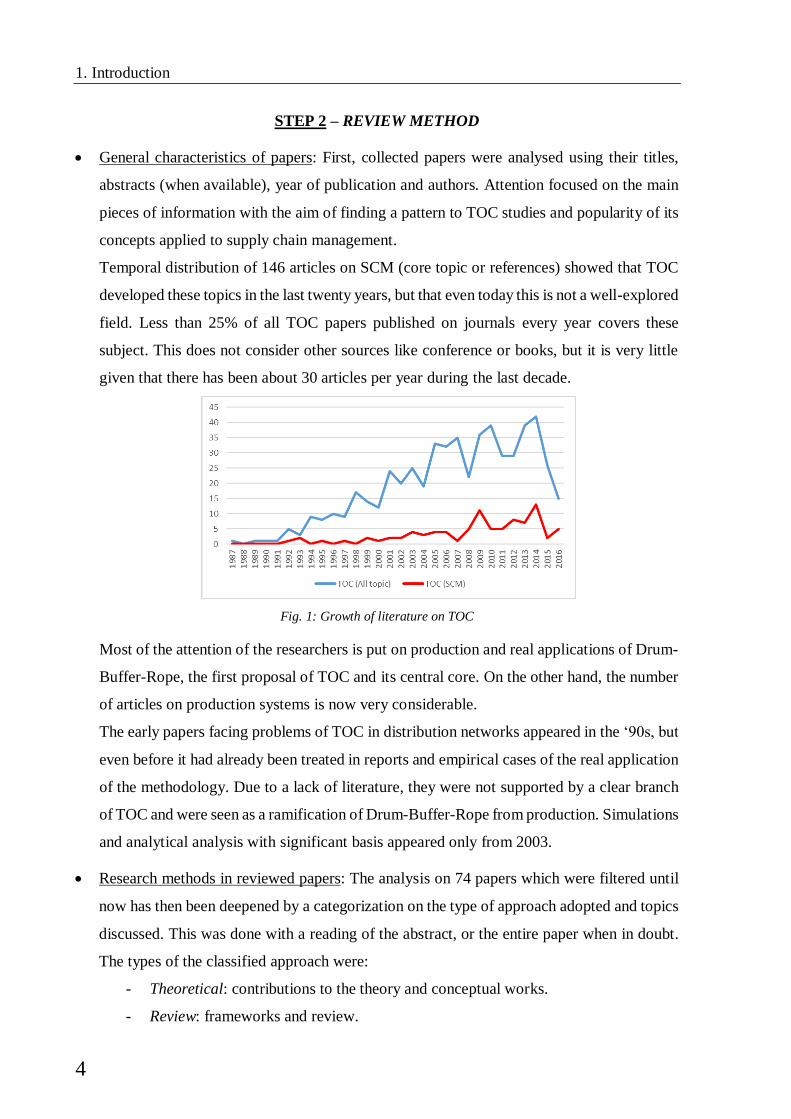
Temporal distribution of 146 articles on SCM (core topic or references) showed that TOC
developed these topics in the last twenty years, but that even today this is not a well-explored
field. Less than 25% of all TOC papers published on journals every year covers these
subject. This does not consider other sources like conference or books, but it is very little
given that there has been about 30 articles per year during the last decade.
Fig. 1: Growth of literature on TOC
Most of the attention of the researchers is put on production and real applications of Drum-
Buffer-Rope, the first proposal of TOC and its central core. On the other hand, the number
of articles on production systems is now very considerable.
The early papers facing problems of TOC in distribution networks appeared in the ‘90s, but
even before it had already been treated in reports and empirical cases of the real application
of the methodology. Due to a lack of literature, they were not supported by a clear branch
of TOC and were seen as a ramification of Drum-Buffer-Rope from production. Simulations
and analytical analysis with significant basis appeared only from 2003.
Research methods in reviewed papers: The analysis on 74 papers which were filtered until
now has then been deepened by a categorization on the type of approach adopted and topics
discussed. This was done with a reading of the abstract, or the entire paper when in doubt.
The types of the classified approach were:
- Theoretical: contributions to the theory and conceptual works.
- Review: frameworks and review.

1. Introduction
5
- Analytical/Quantitative: papers with quantitative analysis or proposing simulations.
- Empirical: mostly focused on a case study.
The papers selected treat supply chains with a various degree of integration between
production and distribution. They were considered of interest when replenishment in a
downstream network was explicitly cited, retailers were involved or the contribution of the
production system was lower. All the simulations and quantitative works were held, seen
the preselection of papers regarding supply chain. However, only three simulations focused
on distribution environments and compared them.
It is worth noting that only one review was completely dedicated to outbound logistics
of TOC and the low number of empirical cases on distribution. Two additional cases were
found thanks to a less structured search. Nonetheless, it is important to report that a greater
number of cases was available googling in Internet but they were not considered because
of their unknown origin.
TOC branches researched: Papers were also classified according to the TOC areas they
discussed. Only when the article contents were linked to these main areas and they were
more than just an isolated citation, have they been taken into consideration:
Papers on
SCM
On TOC
Replenishment
Theoretical 43 10
Review 8 1
Analytical 10 10 (+1)
Empirical 13 2 (+2)
TOTAL 74 23 (+3)
Table 2: Categorization of Papers
(NB. Papers have been classified under more than one research topic)
Table 3: TOC Branches researched
5FS
VA
T A
nal
isys
Bu
ffer
Man
agem
ent
DB
R
(Pro
du
ctio
n)
TOC
Su
pp
ly C
hai
n
Rep
len
ish
men
t
Syst
em
(TO
C-S
CR
S)
Thro
ugh
pu
t
Acc
ou
nti
ng
Thin
kin
g P
roce
ss
21 11 20 20 16 22 13
28% 15% 27% 27% 22% 30% 18%
PerformanceDecision
MakingLogistic ParadigmScheduling and
Control
1. Introduction
6
It seemed that articles on supply chain were well distributed between the areas of TOC.
Authors discussed the topics quite uniformly, so the modern approach on TOC problems
seems to have changed from the past. Indeed, this is not true for other systems addressed
by TOC researches: for example, a great number of empirical cases on TOC production
systems were reported during the years, but their analysis with the principles of Thinking
Process is far more recent. This is coherent with the prospected shift advocated by (K. J.
Watson et al., 2007).
Summarize Papers: Articles referring to replenishment and distribution were read and
outlined below:
(Simatupang et al., 2004) studied how TOC replenishment positively affects the collaboration
between supplier and retailer in reducing the Bullwhip Effect. Contributions on how to manage
demand peaks and buffer levels were brought by (Ronen et al., 2001), while methods of
prioritization of multiple orders in supply chain adopting TOC were studied by (Tang & Cai,
2009).
Simulation regarding TOC are numerous in literature, but most of them are about
production systems and DBR (Walker, 2002). Works that addresses TOC replenishment in
distribution are infrequent and most of them are exploratory kind of studies. One of the first
was (K. Watson & Polito, 2003) with a comparison between TOC and DRP. They created
scenarios using a field research they conducted on multi-product multi-echelon network of a
US manufacturer. The four models dealt with the situation “AS IS” and three possible ways of
its improvement. Baseline model was a decentralized DRP with a lot for lot policy; network
was structured by six retailers and a manufacturer where seasonality and lost sales were
permitted. They simulated other models using DRP under centralization of warehouse and two
implementations of TOC, one aimed to service and one to inventory reduction. Results gave
evidences of the validity of TOC models, with a general improvement of costs and profit
without losing availability.
(Kaijun & Yuxia, 2010) proposed three different TOC policies comparing them with a (s,S,T)
Min-Max policy. First of all, they warned how the model of TOC replenishment was not
formalized in literature, despite being already adopted in various forms by real firms, and the
conflict in determining the replenishment frequency and quantity in central warehouse and
plant. They tried to enhance to most widespread variant in an environment with non-stationary
demand basing on previous researches of (Yuan et al., 2003). Their conclusions showed that
1. Introduction
7
customizing the model to the context provided the better performance and it can also outperform
the Min-Max policy.
A model inspired to the classic Beer Game is proposed by (Costas et al., 2015). It is a single
product linear supply chain composed by five actors. They compared an Order-Up-To policy
(r,S) with a variant of TOC replenishment based on an agent-based approach, a branch of
artificial intelligence.
(Jafarnejad et al., 2016) studied simulation models comparing JIT, TOC and Mixed Integer
Programming (MIP) on the optimization of orders across supply chain. They tried to maximize
profit by considering ABC logic and due dates of the orders, so that the final results were an
appropriate planning for an optimized allocation.
The problem of order frequency under capacity constraint in plant or warehouses were
addressed by (Wu et al., 2010). The problem consists in the dependency of frequency and lead
time of production from order quantity when these locations are capacity constrained; however,
in TOC replenishment these parameters are considered as given in order to determine the order
quantity. The consequence is that order quantity could not be produced or replenished entirely.
This problem does not exist when plant has enough capacity, so that replenishment frequency
can be as fast as possible. Authors proposed possible solutions with an algorithm for the
simultaneous determination of both parameters. The same authors suggested prolongations of
replenishment frequency in another paper (Wu et al., 2012) and how to moderate impact of the
increment in inventory of low frequency (Jiang et al., 2013). The problem had great attention
and other procedures based on swarm particle optimization, genetic algorithm (Jiang & Wu,
2013b) and optimization models (Jiang & Wu, 2013a) were developed refining the solution.
Later, some papers formalized the knowledge on TOC in distribution and downstream of
supply chains (Souza & Pires, 2010) and new approaches emerged. (Leng & Chen, 2012) using
a genetic algorithm to improve coordination and peak management between members of the
supply chain, while (Tabrizi et al., 2012) showed the advantages of information sharing in TOC
and how contract management can benefit both vendor and retailer. (Tsou, 2013) explored
strategies of detection of demand changes with a collaborative approach and how this can
improve the efficiency of Dynamic Buffer Management.
Recently some authors developed strategies mixed with TOC and hybrid methodologies;
for example, (Puche et al., 2016) studied the integration of TOC replenishment with practices
of collaboration proposed by Viable System Model. Most of these studies are supported by
specific industries: some empirical cases were presented by (Chang, Chang & Lei, 2014) in
1. Introduction
8
semiconductor and wafer production supply chain. They analysed the characteristics of demand
and products in order to find effective grouping strategies and apply Drum-Buffer-Rope and
TOC replenishment along the supply chain. (Chang, Chang & Huang, 2014) studied the
integration of demand management through forecast with the pull-demand approach of TOC in
the same industry. (Chang et al., 2015) simulated scenarios using this hybrid and comparing
them with statistical policies. (Lawler & Murgolo-Poore, 2011) studied an application of the
theory to supply chains of the gaming industry, while (Dos Santos & Alves, 2015) its
effectiveness in home appliances segment. Other empirical study like (Oglethorpe & Heron,
2013) used tools and concepts of TOC in studying UK food supply chain next to traditional
ones and finally proposed improvement in management of downstream supply chain with TOC
replenishment. Testing of TOC replenishment with online retailers and e-commerce were
investigate by (Sun & Leng, 2013).
1.2 - Gaps Encountered
The last step of the review procedure presents the findings of readings and analysis conducted
on articles:
STEP 3 – REPORTING
1) Incoherency on the meaning of some terms.
Studying TOC sources some discrepancies were found among the definitions adopted by
researchers. This was caused by an evolution of the topic itself, but also by some misleading
interpretations accepted for years. The most evident example is the meaning of TOC
performance measurements; indeed, Throughput, Operating Expenses and Investments are
those used with a wrong meaning more frequently. TOC terms cited in this work are all and
only those referenced by TOCICO dictionary (Cox III et al., 2012). These are the terms
officially accepted today by TOC practitioners in order to give uniformity to researches.
2) Low number of study on supply chain management and on replenishment
solutions.
From the starting point, total number of papers on TOC was not so high, about one thousand.
Of those excluded it was found that most of the literature on TOC is about production, project
management or organizational change. The first two topics are the initial core of Theory of
Constraints so they are well documented and historically they are the most researched. Even
now empirical cases of DBR are reported; it has been the most promising area of TOC for a

1. Introduction
9
long time. The same can be said about project management and methodology of Critical Chain.
The reason behind the development of so many articles on organizational change management
and strategy are exactly opposite. This is chronologically the last area investigated by TOC
researchers so most of the recent papers are dedicated to these topics.
Literature on supply chain management has not received much attention and this is clearly
visible in the low number of articles. Even if it has finally had an increasing visibility, the
research on some topics are really lacking. Distribution is one of them.
3) Excessive focus on initial parameters instead of demand change detection
Researchers focused their attention on how efficiently setting initial parameters of buffer
management in order to provide quicker start-up in real implementation. Papers on this subject
are largely available in literature, because researchers consider the standard method too
simplistic. By the way, all these criteria have a limited effect and only in the initial phase of
implementation, while autoregulation of DBM can provide more benefit on long term.
Researches should focus on implementing effective criteria to detect changes in demand
pattern.
Little literature on TOC in distribution was found, but this is probably linked to the low attention
of TOC in general towards supply chain management. Excluding papers and articles, only two
books report rigorous formulas of TOC replenishment and how it detects demand change. They
are slightly different: the first is similar to classic DBR in production (Cox III & Schleier, 2010),
the other is based on cumulative penetration (Schragenheim et al., 2009). Principles and theory
supporting them do not change, but the second approach seems to have better performances in
real applications. Nonetheless, most of the papers found in literature apply the first method,
probably because it is slightly simpler and similar to the classic DBR.
4) Lack of empirical cases and quantitative analysis.
Only few empirical cases and real application of TOC distribution management were reported
and well documented in literature. Most of the studies are not available or not accepted in
academic database and those existing regard strategic analysis of firms using Five Focusing
Steps or Thinking Processes.
A limited number of simulations was found. Findings on stability of this solution with
constraints like transportation or minimum batch are missing. Reorder point models with a fixed
order quantity were not found, despite they have been the most common simulations of DBR
in a production system for a long time.
1. Introduction
10
Comparison found in a multi-echelon network were conducted with strategies like DRP, Order-
up-To and Min-Max policies. A few simulations compared TOC with JIT, but in a context
highly integrated with production system and marginal attention on distribution network. All
simulations found considered a pattern of demand quite variable, even with demand peaks, but
rarely verifying the behaviour for a pretty stable demand rate. This is one of the main hypothesis
of models like EOQ and it is the pattern of demand where they reach optimal results. Though
EOQ may perform less efficiently with variable demand, it would be interesting verify that
DBM do not degrade its performance in a stable context.
1.3 - Research Questions
The following questions were formulated studying the gaps in literature. They are considered
interesting for an investigation about TOC with simulation tools and focus the aim of the thesis
towards a definite direction:
1) How does TOC perform in a distribution network compared to a Reorder Point
policy?
2) DBM has numerous settings that guide its functioning. Which parameters have
greater influence on performances?
3) Which constraints\variables\context provides more limitations to DBM
performance?
4) What are limits and drawbacks in TOC Pull Replenishment?

11
2. Taxonomy of
Replenishment
Strategies
The following framework has the aim to trace the principal variants of replenishment strategies.
A complete classification is really difficult due to the huge quantity of articles on this subject.
A considerable number of factors influences configurations of a distribution system and
strategies adopted. They have a trade-off with qualitative variables, which multiply the possible
results and complexity of a unique framework.
Replenishment logic affects profitability and goals, like improvement of service level,
minimization of operating costs or inventory investment. A proper strategy has to customize a
standard methodology in relation to context and adapt it to its objectives determining the
variables needed in order to fit the market. Here is presented a taxonomy of standard models
for inventory control and replenishment decisions, with some of the most known variety.
2.1.1 - Push and Pull
Although push and pull systems are assigned precise definitions by APICS (Blackstone Jr.,
2013), it is also notable that many variants exist. By definition:
Push: “a system for replenishing field warehouse inventories where replenishment
decision making is centralized”. In a push logic, inventory planning is responsibility of
a unique planner and replenishments are allocated to downstream locations; centralized
forecasts and allocations to downstream warehouses are typical of push systems.
Pull: “a system for replenishing field warehouse inventories where replenishment
decisions are made at the field warehouse itself”. In a pull logic, every facility maintains
control on local planning and place orders independently from manufacturers or
distributors; a decentralized ordering and demand-driven approach are more distinctive
of pull systems.

2. Taxonomy of Replenishment Strategies
12
In distribution systems, the dividing line between these logics is put where decision making
about replenishment takes place. Other implications of adopting a pull system consist in the
possibility of each facility to choose its own ordering technique and necessity to establish a
solid channel of communication with high quality information. TOC avoids push approach
because this model has a natural predisposition to keep extra stock as close as possible to
customers without a real and manifest demand.
The advantages of a push logic are risk reduction, provided by accumulating inventory at
POS, and economies of scale. Having control on all replenishments in supply chain enables
accurate planning and optimal reorder points. On the other hand, the large amount of stock
implies higher holding costs and obsolescence. The problem firms are more sensible to is the
low flexibility and lack of responsiveness. The pre-allocated inventory cannot cope effectively
with a sudden demand peak and forecasts can prevent this only partially (if correct).
In last decades an increasing number of firms is turning to pull models. Advantages of pull
systems come from a simpler planning and higher inventory turns. Every location is responsible
for its planning, with less efforts of planners at central warehouse. Only the needed quantities
are supplied, so generally overall cost of inventory is lower and stock turnover faster.
Conversely, this decentralized approach makes critics quality of communications and feedback.
A constant monitoring of performance and status is needed for a correct application of
replenishments. Local optimizations are a concrete risk if a correct performance measurement
system is not implemented, partially reducing potential benefits of the model. Pull requires the
quality of transmitted information to be improved while push is more permissive. In a push
strategy information really needed circulating in the network are a small amount and less
essential.
Generally, supply chains use both these types of models, avoiding the consequences of a
radical shift from a pure model. Push approach is useful and preferred in upstream locations
because of a better reliability of forecasts; pull is applied downstream in order to enable
postponement strategies and avoid big amount of inventory. Decoupling points are the
connection between a push upstream and pull downstream, working as interfaces. The
positioning of these points cannot proceed separately from the identification of push/pull
features required by the market. However, once they are in place, some of these characteristics
may be changed to match different requirements. Managerial decisions can change the
behaviour of the system and move decoupling points. A change of this entity requires also a
2. Taxonomy of Replenishment Strategies
13
different strategic view of the system. In this context every supply chain has a mix of push and
pull processes in order to assure agility (Christopher & Towill, 2000).
Push and Pull concepts are applied by numerous techniques in different ways. They are
referred indistinctly to whole systems, policies or simple features of controlling. It is not trivial
to study networks or complex systems and to determine under which direction they are moving,
because their locations can be subject to different pressures.
Despite of where orders are issued in a network and the general classification provide by
definitions, there are methodologies and tools recognized as typical of a pull system more than
others; however, they do not exclude practices and tools of the opposite strategy in the same
system. A supply chain can be temporarily unbalanced towards one of these extremes if
circumstances call for it
(Pyke & Cohen, 1990) propose a partial framework for some common control systems in
order to resolve the ambiguity of terms “push” and “pull”. Their schema follows the definitions
of APICS, studying who has decisional authority, and determines how information flow
through the network. The analysis reveals that MRP and Kanban have features that are not
completely push or pull, though they are considered the quintessential examples of respective
systems. (Hopp & Spearman, 2004) study pull production systems and offer an empirical
alternative of the meaning of these terms. They highlight that an explicit limitation to WIP is
the only feature common to all pull systems and absent in push; also distribution system respects
this observation.
2.1.2 - Statistical Inventory Replenishment
A large variety of systems is treated in literature, each of them with its own specific problems
and a different degree of attention during past years. Numerous solutions were proposed,
implementing new philosophies, hypothesis or counterintuitive algorithms.
Commonly, classifications of replenishment rules are based on review frequency and order
quantity as the two decisions that answer questions like “when” and “how much” an order
should be issued. Other classifications with a higher level of detail were proposed by
(Aggarwal, 1974), (Hollier & Vrat, 1978), (Silver, 1981), (Prasad, 1994) considering also
inventory-related costs, environmental parameters and structure of the system.
Inventory reviewing frequency splits strategies in two broad categories:
- Continuous review: monitoring in every instant trigger points.
- Periodic review: with a fixed frequency of control.

2. Taxonomy of Replenishment Strategies
14
Strategies are classified as hybrid when they mix characteristics from these monitoring method.
Orders size can be either fixed or variable; quantity is fixed when orders are in batch of size
(Q), while it is variable if it is adjusted to make inventory position meet a predetermined
inventory target level (S), generally called base-stock level.
This provides a first partition between policies with variable cycle/fixed order quantity and
fixed cycle/variable order quantity. Inventory position (IP) includes physical inventory actually
on hand, backorders to fulfil and orders from suppliers not arrived yet. It is defined as:
𝐼𝑛𝑣𝑒𝑛𝑡𝑜𝑟𝑦 𝑝𝑜𝑠𝑖𝑡𝑖𝑜𝑛 = 𝑆𝑡𝑜𝑐𝑘 𝑜𝑛 ℎ𝑎𝑛𝑑 + 𝑂𝑢𝑡𝑠𝑡𝑎𝑛𝑑𝑖𝑛𝑔 𝑂𝑟𝑑𝑒𝑟𝑠 − 𝐵𝑎𝑐𝑘𝑜𝑟𝑑𝑒𝑟𝑠
The evaluation of the strategy to adopt is based on the limitation of trade-off between
ordering/reviewing and warehousing costs. Considering demand, we can see that a continuous
approach for low demand and a periodic review for high demand items is frequent. There are
also qualitative characteristics of the supply chain that influence this decision, for example
reliability of the suppliers, the difficulties of taking a complete inventory or the possibility of
order aggregation. A continuous review is more responsive to demand variation and reduces
the level of safety stock, while periodic review has an exposition equal to order frequency
interval. A periodic review opens to some risks but it is usually less expensive and involves less
efforts thanks to the discontinued approach, enabling also a detailed planning. However, today
the cost differences have been reduced progressively because of the new tools of information
technology and results of a continuous or periodic review are very similar for short review
period.
Given the choice between fix or variable, four basic policies are possible (Ross, 2015). The
adopted notation may vary from other literature:
Q = Fixed Order Quantity S = Base stock (MAX)
r = Review Frequency s (often indicated as R) = Order Point (MIN)
Order Quantity
Fix Variable
Review
Frequency
Periodic (r,Q) (r,S)
Continuous (s,Q)
also known as (R,Q) (s,S)
Table 4: Basic Replenishment Strategies

2. Taxonomy of Replenishment Strategies
15
(R,Q) and (s,S) replenishment rules are classified under continuous review and are also called
Reorder Point (ROP) systems. (r,S) policies has a periodic review system, while generally (r,Q)
is of low interest because it is the most rigid. Their logic is described as follows:
(r,Q): a periodic review policy with a fixed order of size Q released every r period. Note
that only order size is fixed, not number of orders, so it is possible to release N orders
of size Q. This limitation usually is related to an EOQ calculation or a transportation
constraint, so it has a low flexibility.
(s,Q) or (R,Q): continuous review policy where N orders of size Q are released every
time IP is equal or less than a minimum quantity s. It often is adopted when supplier
requires ordering in batch, so it is also denoted as (s, nQ). Number of orders depends on
the minimum quantity of batch required so that IP is at least higher than s, but the
maximum value of inventory position is always limited at IP ≤ s + Q (Axsäter, 2015);
the Order Point (OP) is met exactly in s only in a case with constant demand and
continuous review.
(r,S): a periodic review policy commonly referred to as “Order-Up-to” or “Base Stock
Policy”. Every r periods an order is released so that IP once replenished is at least equal
to a maximum value S. Note that ordering in this policy is mandatory and it is
completely independent from actual inventory position.
(s,S): also called “Min-Max” policy. A variable order of size OQ = S – IP is released
every time inventory position is equal or less than a predetermined minimum value s in
order to restore the stock to the max level S. This policy is equivalent to (s,Q) when S
= s + Q. It has a variation called (S-1,S) when it releases order immediately after one
unit is taken.
This classification is the most widely adopted in literature, but reviewing method and triggers
are somehow overlapped. Reviewing method regulates the task of determining inventory
position and how much inventory is in stock; that decides how often inventory is monitored.
On the other hand, trigger outlines how orders are placed and it is not strictly dependent on
inventory position. Indeed, an order could be mandatory because of some contractual
constraints with supplier, so the trigger would be fix. Instead, triggers are variable if linked to
a minimum inventory level (s); when inventory position is equal or less than a certain reorder
point, then an order is placed.
2. Taxonomy of Replenishment Strategies
16
In all the policies above, the instant of identification of actual stock level is the same of
when is possible to release an order. Realistically, it is not always viable; although information
technology can make it possible for most of the products, there are also items that for some
reason record delays between these two events. Seen the importance of Buffer Management for
TOC, it is interesting to add a further distinction between these two parameters and to split the
decisions in order to provide a better comparison. Wensing studies this type of classification
(Wensing, 2011) and identifies combinations of triggers and reviewing methods that do not fit
each others:
Frequency of inventory review (HOW OFTEN)
Size of the order (HOW MUCH)
Triggers for order release (WHEN)
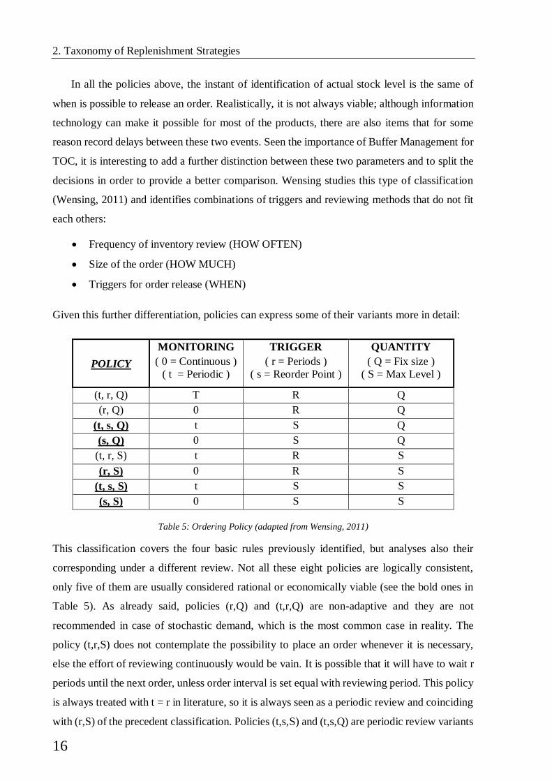
Given this further differentiation, policies can express some of their variants more in detail:
This classification covers the four basic rules previously identified, but analyses also their
corresponding under a different review. Not all these eight policies are logically consistent,
only five of them are usually considered rational or economically viable (see the bold ones in
Table 5). As already said, policies (r,Q) and (t,r,Q) are non-adaptive and they are not
recommended in case of stochastic demand, which is the most common case in reality. The
policy (t,r,S) does not contemplate the possibility to place an order whenever it is necessary,
else the effort of reviewing continuously would be vain. It is possible that it will have to wait r
periods until the next order, unless order interval is set equal with reviewing period. This policy
is always treated with t = r in literature, so it is always seen as a periodic review and coinciding
with (r,S) of the precedent classification. Policies (t,s,S) and (t,s,Q) are periodic review variants
POLICY
MONITORING
( 0 = Continuous )
( t = Periodic )
TRIGGER
( r = Periods )
( s = Reorder Point )
QUANTITY
( Q = Fix size )
( S = Max Level )
(t, r, Q) T R Q
(r, Q) 0 R Q
(t, s, Q) t S Q
(s, Q) 0 S Q
(t, r, S) t R S
(r, S) 0 R S
(t, s, S) t S S
(s, S) 0 S S
Table 5: Ordering Policy (adapted from Wensing, 2011)
2. Taxonomy of Replenishment Strategies
17
where evaluation of inventory is not continuous. This difference enables the coordination of
orders processes compared to the (s,S) and (R,Q).
Numerous variants of these policies have been studied in literature, and it has been noticed
that most of them have hybrid characteristics. It has been demonstrated that under simple
assumptions optimal policies exist in a single-echelon context. (Veinott, 1965) proved
optimality of (R,Q) policy in serial systems when there are no ordering costs and order quantity
is a multiple of Q. Also (s,S) policy is optimal for serial systems, as shown by (Iglehart, 1963)
and (Zheng, 1991). These results have been extended also to assembly systems thanks to
(Rosling, 1989), who proved that serial systems are only a subcategory of them when costs are
linear.
Till this point, only single-echelon systems have been considered. However, supply chains
are formed by the interaction of more actors and warehouses. Optimality of the precedent cases
is not maintained in every multi-echelon systems. Coordination covers a particular role and new
technologies assume a vital role to get clear information. Heuristic approaches are more
common for these systems, because of the great complication of the problem. Distribution
networks may have an arborescent structure with many downstream locations, differently from
serial and assembly systems of production which have at most one successor. In TOC, a similar
research is conducted with the help of VAT analysis, explained in the following paragraphs.
The necessity of a global point of view has led to a differentiation in how stock are viewed.
In ’60s, Clark introduced the distinction between installation stock and echelon stock (Clark &
Scarf, 2004). For a distribution system where typologies of items are the same at every level,
echelon stock is equal to the sum of installation stock at a certain level plus all those
downstream. Inventory position in an installation stock policy regards only local inventory, so
facility N releases an order to N+1 location without considering the whole amount of inventory
already in downstream supply chain. This kind of policy is always nested, linking each level to
the next one. Instead, an echelon stock policy reacts only to the final demand because it
considers the total amount of the downstream stock in inventory position calculation. A problem
to face using echelon stock policy is the number of information needed; although it has a global
point of view, it requires also a constant flow of information from downstream in addition to
local information on inventory position. On the contrary, they are minimal with installation
stock but local optimizations are more likely.
2. Taxonomy of Replenishment Strategies
18
(Axsäter & Rosling, 1993) proved the following propositions related to (R,Q) multi-echelon
policies for serial systems:
1. “An installation stock reorder point policy can always be replaced by an equivalent
echelon stock reorder point policy”.
2. “An echelon stock reorder point policy which is nested can always be replaced by an
equivalent installation stock reorder point policy”.
This means that installation stock policy is a special case of an echelon stock policy for linear
and converging supply chain, similarly to the single-echelon case. The republished work of
(Clark & Scarf, 2004) provides results regarding optimal base-stock policies in serial multi-
echelon systems. They validate this in a finite horizon periodic problem, with unlimited
capacity, no setup cost and linear transportation cost. Later, this has been extended to infinite
horizon or presence of capacity limitation and even to assembly systems, but it is not possible
to state this optimality also for distribution systems. Other results about these systems with
batching orders were brought by (Chen, 2000b).
(Axsäter & Rosling, 1993) shows that optimality of echelon stock is not assured for distribution
system, contrary to cases of serial and assembly systems:
3. “S policies based on the echelon stock are equivalent to S policies based on the
installation stock for general systems”
An optimal approach is not found out in these situations. Base Stock policies are said to be
myopic, however they can reach good results even in this context (Kogan & Shnaiderman,
2011). Generally, a (R,Q) policy offers comparable results in these cases; this is true in
particular for (S-1,S) policy, which is a special case of a (R,Q).
A problem of installation stock policy in multi-echelon system is the “Forrester effect” or
“Bullwhip effect”. The functioning of the policy does not require other information than local
one, so communication could be neglected to a low level. Synchronization and collaboration
between stages of supply chain is one of the most effective way to avoid this backstroke of
installation stock (Ciancimino et al., 2012).
In multi-echelon systems, there are at least three methodologies of common use:
(R,Q) or (s,S) installation stock policy to control each facility, each of them with their
own reorder point and inventory position.

2. Taxonomy of Replenishment Strategies
19
(R,Q) echelon stock policy, considering that calculation of inventory position is slightly
different and require more information.
Kanban policies; they are very similar to an installation stock (R,Q) policy where
backorders are not subtracted from inventory position.
A great variety of simulations is present in literature, each of them focusing on some elements
or introducing new decision variables. (Pérez & Geunes, 2014) considered a single-stage
inventory replenishment model that includes two delivery modes, one cheaper but less reliable
while the other one more expensive and really fast in case of emergency. (E. A. Silver, H.
Naseraldin,D.P.Bischak, 2009) studied an Order-up-To under periodic and continuous review
and presented an approach to determine reorder point and target value using customer fill rate.
A variation of the same model was discussed in (Silver et al., 2012), considering negative
binomial demand. (Handfield et al., 2009) presented a model considering the attitude of
decision maker toward the risk of stocking out during the replenishment period and use a
triangular fuzzy functions for modelling the uncertainty of factors. (Grewal et al., 2015) studied
a dynamic adjustment of decision variables with seasonal demand. They recognize the
advantages of these corrections, but do not link them to Theory of Constraints.
2.1.3 - Time-Phased Techniques: MRP and DRP
A different solution from statistical calculation is to apply a time-phased demand and supply
in a multi-echelon supply chain. (Whybark, 1975) proposed Distribution Requirements
Planning (DRP) as an extension of MRP, while (Stenger & Cavinato, 1979) formalized the
logic moving the same principles of MRP from production to distribution. Their relationship
is really tight because DRP feeds Master Production Schedule, which is itself an input to
MRP. DRP uses the same backward logic of MRP, but it can be applied under either push or
pull logic. Its pull functioning requires some input data:
Inventory Status: on-hand stock available and safety stock level.
Ordering Data: minimum lot size required for an efficient process of replenishment.
Distribution Network Design: required for addressing orders to the correct facilities
and determines lead times.
Bill of Distribution: product structures and dependencies of components undergo an
“implosion” of requirements, instead of an “explosion” of Bill of Materials (BOM) like
in MRP.
2. Taxonomy of Replenishment Strategies
20
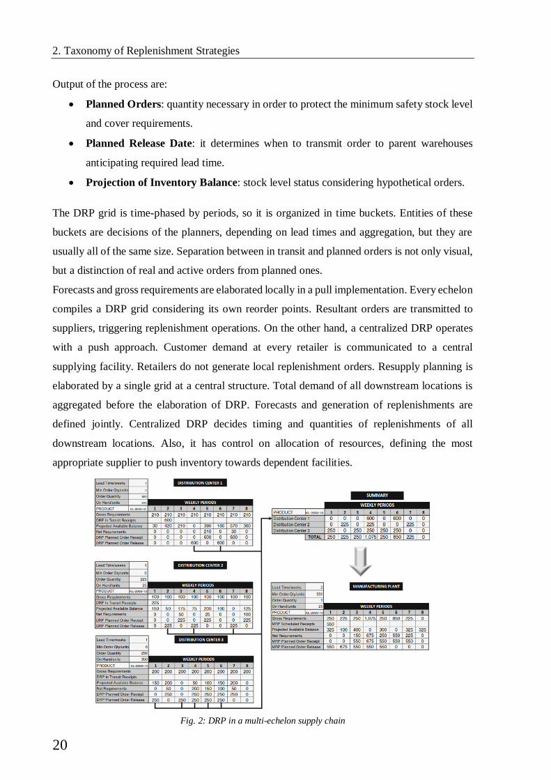
Output of the process are:
Planned Orders: quantity necessary in order to protect the minimum safety stock level
and cover requirements.
Planned Release Date: it determines when to transmit order to parent warehouses
anticipating required lead time.
Projection of Inventory Balance: stock level status considering hypothetical orders.
The DRP grid is time-phased by periods, so it is organized in time buckets. Entities of these
buckets are decisions of the planners, depending on lead times and aggregation, but they are
usually all of the same size. Separation between in transit and planned orders is not only visual,
but a distinction of real and active orders from planned ones.
Forecasts and gross requirements are elaborated locally in a pull implementation. Every echelon
compiles a DRP grid considering its own reorder points. Resultant orders are transmitted to
suppliers, triggering replenishment operations. On the other hand, a centralized DRP operates
with a push approach. Customer demand at every retailer is communicated to a central
supplying facility. Retailers do not generate local replenishment orders. Resupply planning is
elaborated by a single grid at a central structure. Total demand of all downstream locations is
aggregated before the elaboration of DRP. Forecasts and generation of replenishments are
defined jointly. Centralized DRP decides timing and quantities of replenishments of all
downstream locations. Also, it has control on allocation of resources, defining the most
appropriate supplier to push inventory towards dependent facilities.
Fig. 2: DRP in a multi-echelon supply chain
2. Taxonomy of Replenishment Strategies
21
DRP and MRP grids are similar in functioning. They do not calculate inputs like lot size, safety
stock or frequency of replenishment under a predetermined integrated algorithm or a certain
policy. This means that their implementation can be complementary to an existing policy, but
it can also be independent from it, applying their calculations of these inputs rather than using
another method. For example, choice of a lot size can be made by using Economic Order
Quantity, Lot for Lot or the result of a policy.
A great drawback of MRP and DRP is the large computational effort in case of thousands
of items and complex structures. Nonetheless, their logic is simple and effective. Another well-
known problem is “nervousness” of MRP output even for small change in input. A centralized
DRP has this same problem related to instability of input forecast, instead of MPS. ”Freezing”
closest orders is a solution to avoid nervousness.
Contributions to this theme are brought by (Bookbinder & Heath, 1988), with a comparison
of five lot-sizing policies in a multi-level distribution network with stochastic demand. They
find that, contrary to MRP cases in production, DPR performances are greatly influenced by
lot-sizing policies. Within their simulations, they identify the best outcome in Silver-Meal
heuristic (Silver & Meal, 1973). (Martel, 2003) studies rolling planning horizon policies,
discussing the impact of expediting actions on DRP. A complete review on rolling planning is
developed by (Sahin et al., 2013). (Wang, 2009) propose an integration artificial intelligence
and DRP, examining the field of continuous review inventory model with the introduction of a
transformation of fuzzy number into a closed interval. An effective comparison between
DRP/MRP, Reorder Point policy and Kanban is provided (Suwanruji & Enns, 2006). They
simulate multi-echelon supply chain with stochastic demand considering both production and
distribution. Their results highlight that with a seasonal demand DRP/MRP perform best,
followed by Reorder point policies and Kanban. What is more interesting for this thesis, they
argue that performance ranking depends on capacity constraints without seasonality, so they
analyse it with queueing theory: in presence of a constraint, Kanban is the best and DRP/MRP
immediately follow; without evident capacity constraints, Reorder point is the top and
DRP/MRP is even better than Kanban. Similar comparison between MRP, Kanban and Reorder
Point policies is conducted by (Axsäter & Rosling, 1994). In particular, they demonstrate that
MRP is dominant over installation stock policy for general inventory system and it is equivalent
to a reorder point policy if replenishments are instantaneous. As already said for statistical
techniques, they argue that a mere classification of MRP and DRP under the name of push and
pull is unclear. They demonstrate that:

2. Taxonomy of Replenishment Strategies
22
1. For a general inventory system, an MRP system can give the same control as any
installation stock reorder point system.
2. For serial and assembly systems, MRP can work as any echelon stock reorder point
system.
2.1.4 - Lean Philosophy in Distribution
Today the Lean approach has a large diffusion in numerous industries and business. Its origins
dates back to Japan of post Second World War and it has been largely influenced by this context
strongly constrained by resources. Principles of Toyota Production System (Ohno, 1988)
blended Ford’s mass production and Japanese culture and was recognized as a new approach.
TPS had a great success in manufacturing and Just-in-Time concept became popular among
western companies. Lean Thinking (Monden, 1998; Womack & Jones, 1996) is one of the
responsible for the shift from a push-based production to a pull-based approach. Philosophy of
JIT expanded and was applied on other enterprise areas, until it overtook company borders with
applications on supply chains. This evolution involved even environments completely different
from manufacturing, like service operations (Swank, 2003).
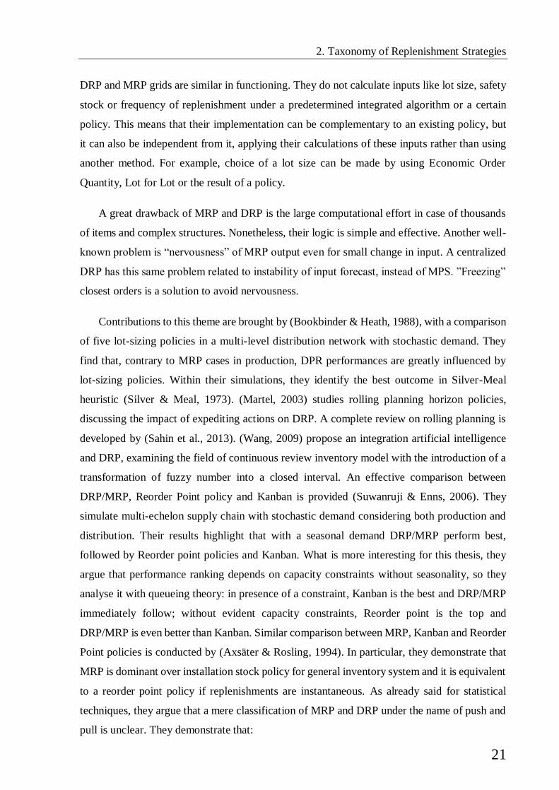
Lean Principles are the key elements of Lean
philosophy. It is visible the similarity of these
principles with Five Focusing Steps of TOC, even if
they focus on different aspects: TOC controls
constraints that limit throughput, while Lean
eliminates waste and variability in order to level the
flow. Both of them are customer oriented and pull-
based, but the way chosen to achieve this is opposite:
for example, Lean focuses on balancing; on the other
hand, TOC accepts imbalance if it can maximize
throughput.
Despite developments of the theory and the presence of an incredible number of cases of
study, (Anand & Kodali, 2008) note that theoretical concepts behind Lean Supply Chain could
be furtherly developed. Lean Distribution is a logical extension of Lean Supply chain and Lean
Logistics (Zylstra, 2005), so it is not a radically new concept and could benefit of those same
studies. A definition of Lean Distribution under Lean Thinking philosophy is “minimizing
waste in the downstream supply chain, while making the right product available to the end
Fig. 3: Five Lean Principles

2. Taxonomy of Replenishment Strategies
23
customer at the right time and location” (Reichhart & Holweg, 2007). Unfortunately, this area
of Lean has less evidence in literature, while relationships with suppliers have a predominant
role and have been deeply investigated (MacDuffie, 1997).
Compared to other branches of Lean, authors have been interested in the Supply Chain
Management only lately, facing problems of responsiveness (Fisher et al., 1994; Fisher, 1997).
(Manzouri & Rahman, 2013) investigate how supply chain management theories adapt to lean
principles. (Reichhart & Holweg, 2007) argue that contributions of Lean focusing specifically
on distribution operations and applications to downstream are really scarce in literature. They
retrieve a possible cause in the conflict between lean principle of level scheduling (heijunka)
and the excessive variability of market and demand of final customers; inevitably, a lean
distribution system collides with buffering against demand volatility. More recently (González-
R et al., 2013) discuss the slow diffusion of JIT in downstream locations in pull-based supply
chains, but highlighting an increment of studies on this subject. They propose a methodology
for implementation of short-term control in a multi-echelon supply chain with a sequential-
iterative mechanism to optimize the single-card Kanban loops. An example of a recent study
on distribution and retail sector is (Daine et al., 2011). (Martínez Jurado & Moyano Fuentes,
2014) show empirical evidence that researchers have focused on analysing ‘upstream’ Lean
principles and practices, while little work has been done on analysing how they have been
applied ‘downstream’. Despite the lack of theoretical studies on this matter, numerous cases of
study have been reported of successful implementations of JIT in distribution. Some examples
are (Kiff, 2000) about automotive dealers and their customers, (Jaca, 2012) in distribution
centres and retail sector with insight on change management and (Lehtonen & Holmström,
1998) in paper industry.
(Olhager, 2002) analyses advantages of JIT in supply chain management and potential
benefit of balancing lead times between locations. He suggests that lead-time conformity in
every stage of supply chain is more important than equivalence between processing time in
order to achieve good lead-time performance. He supports the analysis of lead-time efficiency
as key measure of a good implementation of JIT in supply chains. However, a distribution
system has to manage extreme variability and it cannot work in efficient way without a certain
amount of inventory placed strategically along the network. This trade-off is faced by
(Christopher, 2000) and (Christopher & Towill, 2000) with the proposal of a shift from Lean
Supply Chain to an Agile Supply Chain, aimed to a better availability.
Themes linked to supply chain management are growing, particularly on green practices,
but most of them are focused on the relations between suppliers and the focal company.

2. Taxonomy of Replenishment Strategies
24
For example, (Vachon & Klassen, 2006) study how green practices are related to supply chain
characteristics, making a distinction between suppliers and customers. Downstream integration
and extensions of collaborative paradigm to customers are investigated, but they highlight that
these practices are strong only on a strategic level and less effective on a tactical level. Thanks
to surveys and empirical evidence, they find out that most firms believe it is more productive
sharing and monitoring with suppliers on environmental measures, despite the growing
attention of customers on these topics.
Lean manages buffers in a manner sharply different from TOC. In a Lean system they are
placed between every node and replenished of the quantity required by downstream location;
they absorb demand variations in order to minimize fluctuations on the flow. In contrast, TOC
places consistent buffers only in strategic locations and it uses an additional regulation
mechanism of buffer size next to normal replenishment cycle.
Kanban cards are the most common technique to trigger inventory replenishment in a Just-
in-Time implementation. Many variations of the Kanban system are present in literature.
Originally, Toyota adopted a double-card Kanban system (Sugimori et al., 1977), but numerous
alternatives have been developed in order to fit a wide range of systems and surpass its
restrictions. Their peculiarities aim to better performance, maintaining Kanban logic;
development of new communication technologies opened to a progressive evolution of Kanban.
(Lage Junior & Godinho Filho, 2010) studied 32 typologies of Kanban, from the original
double-card Kanban to E-Kanban, without physical cards circulating.
Kanban policy operates in a similar manner to a (R,Q) policy (Axsater et al., 1999; Axsäter,
2015). If we consider a system with N containers / Kanban of size Q and one container serving
per time, then N-1 containers are always full. Actual inventory position will be equal to (N-
1)∙Q plus the remaining of container serving in that moment; a new order is triggered every
time a container is empty and its Kanban released. The behaviour of this simple case is the same
of a (R,Q) policy with R = (N-1)∙Q and container size identical to order size. The real difference
between the two models is that Kanban put an explicit limit also to the total number of
outstanding orders; no more orders are released when their number reaches N, that is the
maximum number of Kanban cards in the system.
Even base-stock policies have similarity with Kanban (Veatch & Wein, 1994). (S-1,S) is a
variation of a Min-Max policy with a continuous review process that releases an order of one
unit as another item is taken away. Ideally, Kanban is reduced to a single piece when Lean
achieves the objective of One-piece-flow processes. (S-1, S) policy operates in the same manner
when they are near this upper limit.

25
3. TOC Principles
and Paradigms
In the late ‘70s, Eliyahu M. Goldratt formulated first principles and basis of Theory of
Constraints (TOC); its development started with the introduction of a scheduling and control
software known as Optimized Production Technology (OPT), but only by ‘80s the overall
concept became known as TOC (Goldratt & Cox, 2004; Spencer & Cox III, 1995).
It started as a production philosophy but gradually expanded to every aspect of business: it
refined itself from production floor and logistical system for material flow Drum-Buffer-Rope
(DBR) till a comprehensive approach called Thinking Processes (TP), which can analyse
constraints in every division of a firm. Currently, these Thinking Processes are the most
advanced paradigm of TOC.
TOC has three major interrelated components (Boyd & Gupta, 2004; Inman et al., 2009;
Rahman, 1998): a philosophy that defines the production/logistics paradigm, which covers the
continuous improvement with Five Focusing Steps, VATI analysis, Drum-Buffer-Rope
scheduling system and Buffer Management control system; a methodology to deal with problem
solving and decision making, where Thinking Processes are the key tools in order to examine
methodically complex situations; a new performance measurement system, different from
traditional cost accounting, called Throughput Accounting.
Fig. 4: TOC Elements
3. TOC Principles and Paradigms
26
In literature are present numerous frameworks that facilitate comparison with other
methodologies of operational research and management science. Refer to the work of Davies,
Mabin and Balderstone (Davies et al., 2005) for a classification of TOC and its tools in the most
known frameworks and for further comparisons with other important philosophies.
Apart these development, TOC had great numbers of critics since its first appearance. (K. J.
Watson et al., 2007) identified the most relevant of them, highlighting how most part have been
resolved nowadays. Major points are:
Results not always optimal, but nonetheless feasible and immediately viable.
Ambiguity on some basic definitions.
Lack of methodology and structure in many studies.
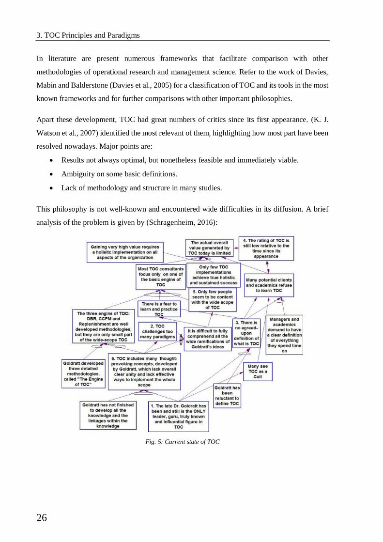
This philosophy is not well-known and encountered wide difficulties in its diffusion. A brief
analysis of the problem is given by (Schragenheim, 2016):
Fig. 5: Current state of TOC

3. TOC Principles and Paradigms
27
3.1 - TOC Glossary
3.1.1 - Constraints
TOC defines “constraint” everything that prevents a firm from achieving its goal and obtaining
higher performances. A basic assumption of TOC is that every system has at least one
constraint; otherwise, it conducts to the absurd that a system would be infinitely capable
(Goldratt & Fox, 1986).
There are two large categories of constraints, internal and external; indeed, internal ones can be
further defined:
Physical (internal): they are the physical capacity limit; every resource could be a
Capacity Constrained Resource (CCR) limiting the output, while raw materials, WIP
and any other goods necessary to process are Material Constraints (MC). Usually they
are very common on shop floor in form of production bottlenecks. Physical constraints
are the simplest to solve and elevate.
Policies (internal): they are rules and restraints that a firm puts to itself to limit wrong
or maverick behaviours and make its processes and procedures respected; they also
strongly affect a good decision making and most of the time they increase bureaucracy.
Market (external): the existing system is unable to cope with demand from the market
itself, so strong and deeper improvements are necessary. It can depend on a high level
of demand and too small capacity or bad buffer management.
This means that the widely known production bottlenecks are only a particular class of
constraints, while policies are more widespread and limiting in every organization.
3.1.2 - Buffers
They may be time, stock, capacity, space or money buffers and are strategically located to
protect the system from disruption (Cox III et al., 2012). Stock Buffers are used both in MTS
and MTO environments, while Time Buffers are specific of MTO context. In DBR they are
categorized as Constraint, Assembly and Shipping Buffers. Usually, Times Buffers are time in
advance that materials are released before they are planned to be processed. The characteristic
of TOC is that this type of buffer is not used to protect a planning or respect machine schedules
during the process, but to assure that the entire system is on time for a due date. More generally,
a Time Buffer is defined as a liberal estimate of the manufacturing lead time from one control

3. TOC Principles and Paradigms
28
point to another, which can be a material release point, a CCR or a shipping dock. They are
“liberal estimation” because this implies that both manufacturing time and a reasonable safety
time are included. For example, in case of Shipping Buffers this means that usually they are not
larger than the quoted lead time for customer in MTO context (Schragenheim et al., 2009).
Three types of buffers are identified:
Constraint Buffer: liberal estimation of the manufacturing lead time from the release
of raw materials to the site of the CCR; this typology of buffer is present only if there is
an internal CCR to the process and protects the constraint from starvation.
Assembly Buffer: liberal estimation of the manufacturing lead time from the release of
raw materials to an assembly point where CCR parts and non-CCR parts are combined.
Its presence depends on routing and bill of material of the item, it could be unnecessary.
Shipping Buffer: liberal estimation of the manufacturing lead time from the CCR to
the completion of an order. It protects from any statistical fluctuation along the process.
Time Buffers cannot be directly related with the physical presence of stock on the shop floor.
Naturally there will be more orders in the process, but they are not assigned to a specific
location. This is why Time Buffer can be computed only between two control points. The real
value of these buffers depends on time they need to be processed and the overall level of
variability of the system.
Fig. 6: Types of buffer (adapted from Schragenheim & Dettmer, 2001)
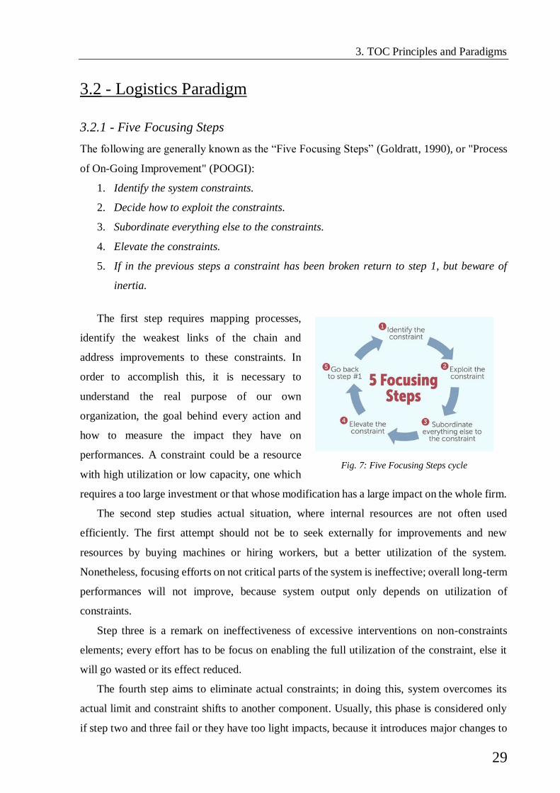
3. TOC Principles and Paradigms
29
3.2 - Logistics Paradigm
3.2.1 - Five Focusing Steps
The following are generally known as the “Five Focusing Steps” (Goldratt, 1990), or "Process
of On-Going Improvement" (POOGI):
1. Identify the system constraints.
2. Decide how to exploit the constraints.
3. Subordinate everything else to the constraints.
4. Elevate the constraints.
5. If in the previous steps a constraint has been broken return to step 1, but beware of
inertia.
The first step requires mapping processes,
identify the weakest links of the chain and
address improvements to these constraints. In
order to accomplish this, it is necessary to
understand the real purpose of our own
organization, the goal behind every action and
how to measure the impact they have on
performances. A constraint could be a resource
with high utilization or low capacity, one which
requires a too large investment or that whose modification has a large impact on the whole firm.
The second step studies actual situation, where internal resources are not often used
efficiently. The first attempt should not be to seek externally for improvements and new
resources by buying machines or hiring workers, but a better utilization of the system.
Nonetheless, focusing efforts on not critical parts of the system is ineffective; overall long-term
performances will not improve, because system output only depends on utilization of
constraints.
Step three is a remark on ineffectiveness of excessive interventions on non-constraints
elements; every effort has to be focus on enabling the full utilization of the constraint, else it
will go wasted or its effect reduced.
The fourth step aims to eliminate actual constraints; in doing this, system overcomes its
actual limit and constraint shifts to another component. Usually, this phase is considered only
if step two and three fail or they have too light impacts, because it introduces major changes to
Fig. 7: Five Focusing Steps cycle

3. TOC Principles and Paradigms
30
the system. Contrary to common sense, TOC views constraints as positive because their
presence establish actual performance and elevate them is a source of opportunities (Rahman,
1998). Last step completes the loop guarding from inertia; this is a cyclic process where
changing is the norm, while stopping in a steady state prevents from further improvements.
3.2.2 - VAT Analysis
VAT Analysis studies the flowing of parts, materials and work through plants and supply chain.
This mapping technique permits a good level of synthesis, but it gives also an overview on the
whole system, providing a valid support in decisions of how to exploit the constraint and
subordinate non-constraints resources through the determination of system control points
(gating, convergent, divergent, constraints and shipping points). Its application should precede
DBR and Buffer Management implementation, avoiding occasional local optimization.
This approach recognises three types of basic configurations that can be mixed and
modified to describe systems. This categorization is based upon the nature of the dominant
material flows, products routings and bill of materials; it provides information on level of
variety at each stage and how much it explodes or reduces compared to the number of
components and assembly parts. Usually, graphical representations of flows are somehow
similar to V, A, T letters:
Recognizing the type of system and its workflow permits a better study of critical points at
different levels. Originally it developed for the study of plants and facility, afterwards its scope
was expanded to the entire Supply Chain networks. Lockamy explains the actions that this
framework suggests in implementation of DBR and Buffer Management referring to divergence
and convergence points (Lockamy, 2008):
Fig. 8: Network Typologies in VATI Analysis
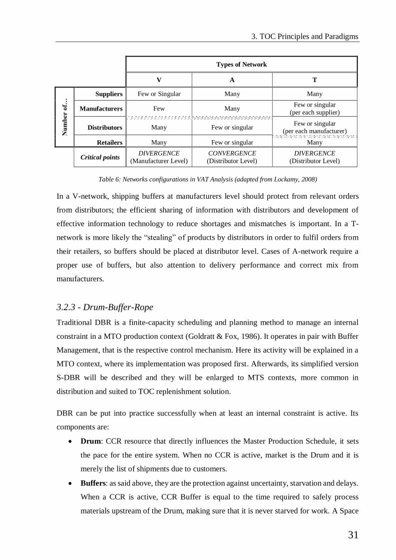
3. TOC Principles and Paradigms
31
In a V-network, shipping buffers at manufacturers level should protect from relevant orders
from distributors; the efficient sharing of information with distributors and development of
effective information technology to reduce shortages and mismatches is important. In a T-
network is more likely the “stealing” of products by distributors in order to fulfil orders from
their retailers, so buffers should be placed at distributor level. Cases of A-network require a
proper use of buffers, but also attention to delivery performance and correct mix from
manufacturers.
3.2.3 - Drum-Buffer-Rope
Traditional DBR is a finite-capacity scheduling and planning method to manage an internal
constraint in a MTO production context (Goldratt & Fox, 1986). It operates in pair with Buffer
Management, that is the respective control mechanism. Here its activity will be explained in a
MTO context, where its implementation was proposed first. Afterwards, its simplified version
S-DBR will be described and they will be enlarged to MTS contexts, more common in
distribution and suited to TOC replenishment solution.
DBR can be put into practice successfully when at least an internal constraint is active. Its
components are:
Drum: CCR resource that directly influences the Master Production Schedule, it sets
the pace for the entire system. When no CCR is active, market is the Drum and it is
merely the list of shipments due to customers.
Buffers: as said above, they are the protection against uncertainty, starvation and delays.
When a CCR is active, CCR Buffer is equal to the time required to safely process
materials upstream of the Drum, making sure that it is never starved for work. A Space
Types of Network
V A T
Nu
mb
er o
f… Suppliers Few or Singular Many Many
Manufacturers Few Many Few or singular
(per each supplier)
Distributors Many Few or singular Few or singular
(per each manufacturer)
Retailers Many Few or singular Many
Critical points DIVERGENCE
(Manufacturer Level)
CONVERGENCE
(Distributor Level)
DIVERGENCE
(Distributor Level)
Table 6: Networks configurations in VAT Analysis (adapted from Lockamy, 2008)
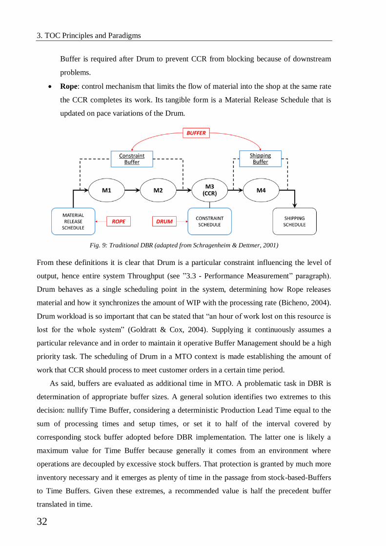
3. TOC Principles and Paradigms
32
Buffer is required after Drum to prevent CCR from blocking because of downstream
problems.
Rope: control mechanism that limits the flow of material into the shop at the same rate
the CCR completes its work. Its tangible form is a Material Release Schedule that is
updated on pace variations of the Drum.
From these definitions it is clear that Drum is a particular constraint influencing the level of
output, hence entire system Throughput (see ”3.3 - Performance Measurement” paragraph).
Drum behaves as a single scheduling point in the system, determining how Rope releases
material and how it synchronizes the amount of WIP with the processing rate (Bicheno, 2004).
Drum workload is so important that can be stated that “an hour of work lost on this resource is
lost for the whole system” (Goldratt & Cox, 2004). Supplying it continuously assumes a
particular relevance and in order to maintain it operative Buffer Management should be a high
priority task. The scheduling of Drum in a MTO context is made establishing the amount of
work that CCR should process to meet customer orders in a certain time period.
As said, buffers are evaluated as additional time in MTO. A problematic task in DBR is
determination of appropriate buffer sizes. A general solution identifies two extremes to this
decision: nullify Time Buffer, considering a deterministic Production Lead Time equal to the
sum of processing times and setup times, or set it to half of the interval covered by
corresponding stock buffer adopted before DBR implementation. The latter one is likely a
maximum value for Time Buffer because generally it comes from an environment where
operations are decoupled by excessive stock buffers. That protection is granted by much more
inventory necessary and it emerges as plenty of time in the passage from stock-based-Buffers
to Time Buffers. Given these extremes, a recommended value is half the precedent buffer
translated in time.
Fig. 9: Traditional DBR (adapted from Schragenheim & Dettmer, 2001)
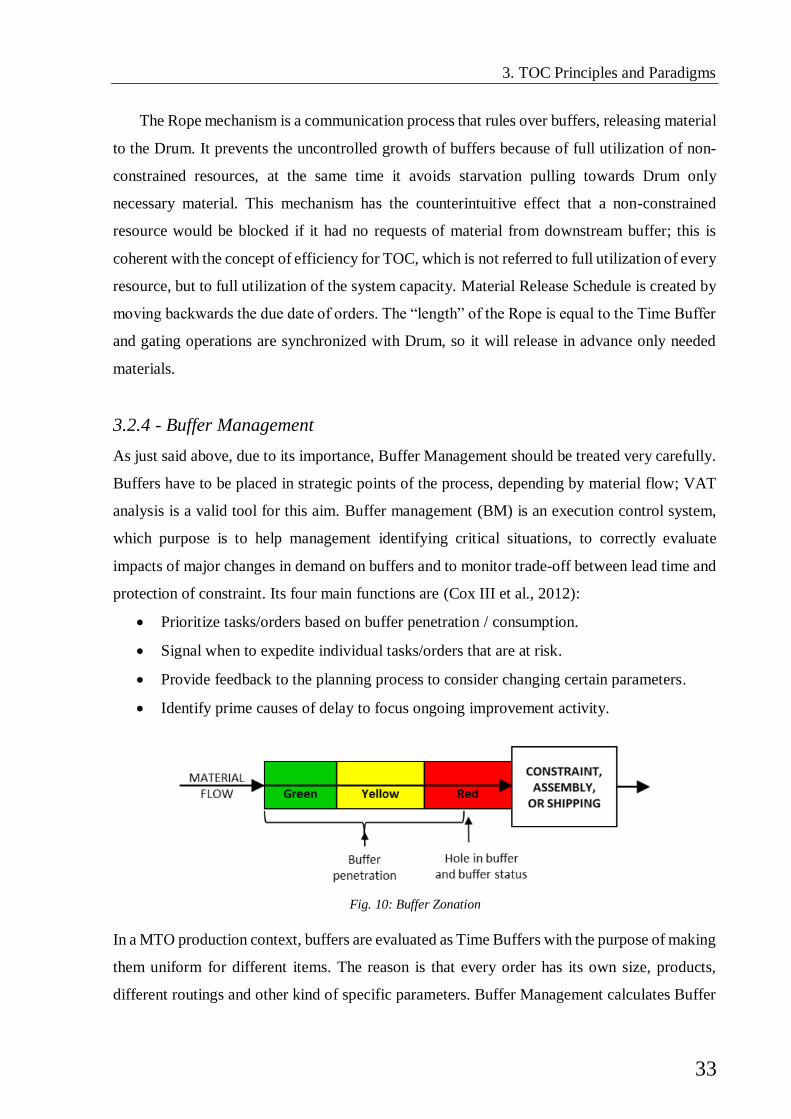
3. TOC Principles and Paradigms
33
The Rope mechanism is a communication process that rules over buffers, releasing material
to the Drum. It prevents the uncontrolled growth of buffers because of full utilization of non-
constrained resources, at the same time it avoids starvation pulling towards Drum only
necessary material. This mechanism has the counterintuitive effect that a non-constrained
resource would be blocked if it had no requests of material from downstream buffer; this is
coherent with the concept of efficiency for TOC, which is not referred to full utilization of every
resource, but to full utilization of the system capacity. Material Release Schedule is created by
moving backwards the due date of orders. The “length” of the Rope is equal to the Time Buffer
and gating operations are synchronized with Drum, so it will release in advance only needed
materials.
3.2.4 - Buffer Management
As just said above, due to its importance, Buffer Management should be treated very carefully.
Buffers have to be placed in strategic points of the process, depending by material flow; VAT
analysis is a valid tool for this aim. Buffer management (BM) is an execution control system,
which purpose is to help management identifying critical situations, to correctly evaluate
impacts of major changes in demand on buffers and to monitor trade-off between lead time and
protection of constraint. Its four main functions are (Cox III et al., 2012):
Prioritize tasks/orders based on buffer penetration / consumption.
Signal when to expedite individual tasks/orders that are at risk.
Provide feedback to the planning process to consider changing certain parameters.
Identify prime causes of delay to focus ongoing improvement activity.
In a MTO production context, buffers are evaluated as Time Buffers with the purpose of making
them uniform for different items. The reason is that every order has its own size, products,
different routings and other kind of specific parameters. Buffer Management calculates Buffer
Fig. 10: Buffer Zonation
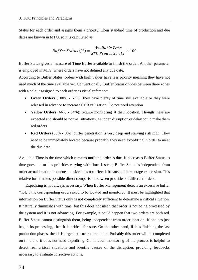
3. TOC Principles and Paradigms
34
Status for each order and assigns them a priority. Their standard time of production and due
dates are known in MTO, so it is calculated as:
𝐵𝑢𝑓𝑓𝑒𝑟 𝑆𝑡𝑎𝑡𝑢𝑠 (%) =𝐴𝑣𝑎𝑖𝑙𝑎𝑏𝑙𝑒 𝑇𝑖𝑚𝑒
𝑆𝑇𝐷 𝑃𝑟𝑜𝑑𝑢𝑐𝑡𝑖𝑜𝑛 𝐿𝑇× 100
Buffer Status gives a measure of Time Buffer available to finish the order. Another parameter
is employed in MTS, where orders have not defined any due date.
According to Buffer Status, orders with high values have less priority meaning they have not
used much of the time available yet. Conventionally, Buffer Status divides between three zones
with a colour assigned to each order as visual reference:
Green Orders (100% - 67%): they have plenty of time still available or they were
released in advance to increase CCR utilization. Do not need attention.
Yellow Orders (66% - 34%): require monitoring at their location. Though these are
expected and should be normal situations, a sudden disruption or delay could make them
red orders.
Red Orders (33% - 0%): buffer penetration is very deep and starving risk high. They
need to be immediately located because probably they need expediting in order to meet
the due date.
Available Time is the time which remains until the order is due. It decreases Buffer Status as
time goes and makes priorities varying with time. Instead, Buffer Status is independent from
order actual location in queue and size does not affect it because of percentage expression. This
relative form makes possible direct comparison between priorities of different orders.
Expediting is not always necessary. When Buffer Management detects an excessive buffer
“hole”, the corresponding orders need to be located and monitored. It must be highlighted that
information on Buffer Status only is not completely sufficient to determine a critical situation.
It naturally diminishes with time, but this does not mean that order is not being processed by
the system and it is not advancing. For example, it could happen that two orders are both red.
Buffer Status cannot distinguish them, being independent from order location. If one has just
begun its processing, then it is critical for sure. On the other hand, if it is finishing the last
production phases, then it is urgent but near completion. Probably this order will be completed
on time and it does not need expediting. Continuous monitoring of the process is helpful to
detect real critical situations and identify causes of the disruption, providing feedbacks
necessary to evaluate corrective actions.
3. TOC Principles and Paradigms
35
Coloured tag orders give useful information about the adequacy of Production Lead Time.
An equilibrated amount of green, yellow and also red orders is necessary. Too much Green
Orders indicate a too large batching, while predominant Red Orders are signal of too small
batch. The system will be regulated by adapting batch size to contingency, meaning it is
possible that inventory will be increased under some circumstances. This reflect precisely the
subordination of everything else to the protection of CCR.
These general indications seem in contrast with the importance of Buffer Management, but
they are coherent with the main idea of TOC that few indicators avoid conflicts and
misinterpretations, so contexts with high complexity need clearer information.
3.3 - Performance Measurement
Throughput Accounting is an area of TOC that has been exposed to critics more than others.
Definitions of new performance measurements were given confusedly and usually they mixed
Traditional Accounting terminology with TOC metrics. This problem affected a large number
of the first articles, books and papers on TOC. Today this problem has been solved establishing
a unique dictionary for TOC (Cox III et al., 2012).
3.3.1 - Throughput Accounting
Increasing complexity triggers the necessity of new metrics and performance assessments. TOC
approach is to face complexity with even simpler metrics which permit to take decisions on
clear information, otherwise data overflow can paralyze the process. Other approaches try to
get the whole range of the problem. They enlarge the scope using large performance
dashboards. Indeed, their effectiveness depends on a good design phase and continuous
maintenance. Also skills of the readers influence their success; ability in interpreting qualitative
factors, besides quantitative ones, is not a given. Such a system usually does not focus on less
than ten measures and clean data are also quite difficult to obtain for some of them (Nørreklit,
2000).
The aim of TOC is to concentrate efforts on few simple measurements avoiding the
possibility of bad behaviours or opportunism, which can be inducted by misinterpretation or
contradictory metrics. “Throughput accounting” is proposed to provide a better explanation of
financial and operative aspects, because traditional accounting methods in decision making are
3. TOC Principles and Paradigms
36
not considered effective with such a complexity. The basic set of operational measurements
includes (Bragg, 2007):
Throughput (T): “the rate at which the system generates money through sales”; output
which is produced and sold. Pieces not sold become inventory. In calculating
Throughput, TOC accounts the part of total variable costs (TVC) that depends from sold
products. The consequence is that generally throughput measures are higher than gross
margin from traditional cost accounting. In traditional cost accounting this measurement
is a contribution margin considering only totally avoidable costs; both approaches
suggest it for a better decision making in case of product-mix definition, acceptation of
extra-orders and make-or-buy decisions (Azzone et al., 2011). TOC proposes the use of
a “Throughput per unit of constraint time” in order to respect the usage of CCR and be
effective considering the configuration of the system.
Operating expenses (OE): “all the money the system spends in turning inventory into
throughput”. It includes company costs like overhead, semi-variable and not totally
avoidable costs (e.g. direct and indirect labour, supplies, MRO, scrap…), but also costs
incurred due the passing time (e.g. depreciation, carrying cost). Today is usual hiring
workforce with a contractual form that makes workers a fixed resource; they cannot be
hired and fired following market oscillation and even if a production line is blocked they
will be paid. Piecework is a rare case where direct labour is not accounted as operating
expense, but as a truly variable cost. Direct labour would not be considered unless
employees were paid only if an item is produced.
Inventory (or investment) (I): “all the money invested in things the system intends to
sell”. It includes every physical inventory intended to be sold; so finished products,
tools, WIP, buildings, capital equipment, furnishing, but also knowledge products like
patents and technology licenses if they are going to be sold. The term “investment” has
been adopted as synonymous with inventory to solve this misunderstanding.
These three measurements are defined in a very plain and simple way in order to be the most
understandable and less arguable possible. In TOC there are only three categories of cost: total
variable costs, investments/inventory and operating expense. Investments and Operating
Expenses are defined with reference to the destination of the costs: for example, a building is
an investment and its depreciation is an operating expense. Actually, definitions of I and OE
eliminate difficulties in accounting value added, which is not purposely assessed by TOC
(Goldratt & Cox, 2004). Generally, TOC does not distinct between direct and indirect labour
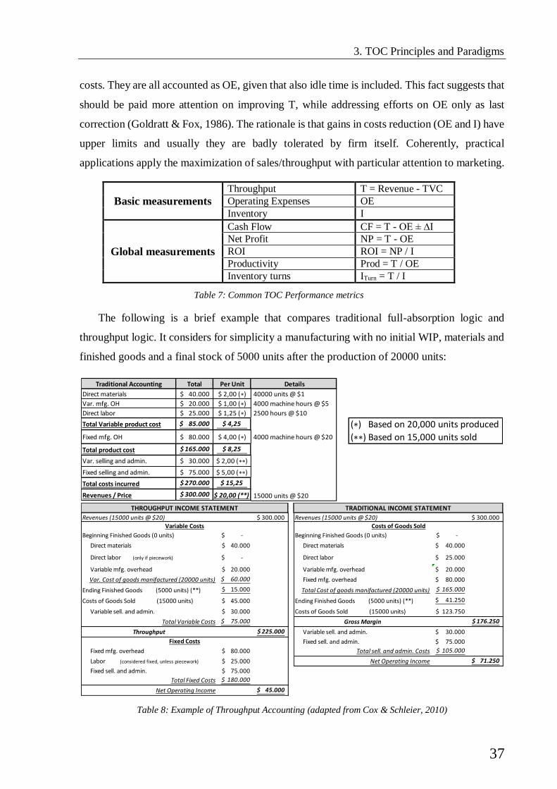
3. TOC Principles and Paradigms
37
costs. They are all accounted as OE, given that also idle time is included. This fact suggests that
should be paid more attention on improving T, while addressing efforts on OE only as last
correction (Goldratt & Fox, 1986). The rationale is that gains in costs reduction (OE and I) have
upper limits and usually they are badly tolerated by firm itself. Coherently, practical
applications apply the maximization of sales/throughput with particular attention to marketing.
The following is a brief example that compares traditional full-absorption logic and
throughput logic. It considers for simplicity a manufacturing with no initial WIP, materials and
finished goods and a final stock of 5000 units after the production of 20000 units:
Basic measurements
Throughput T = Revenue - TVC
Operating Expenses OE
Inventory I
Global measurements
Cash Flow CF = T - OE ± ∆I
Net Profit NP = T - OE
ROI ROI = NP / I
Productivity Prod = T / OE
Inventory turns ITurn = T / I
Table 7: Common TOC Performance metrics
Table 8: Example of Throughput Accounting (adapted from Cox & Schleier, 2010)
Traditional Accounting Total Per Unit Details
Direct materials 40.000$ $ 2,00 (∗) 40000 units @ $1
Var. mfg. OH 20.000$ $ 1,00 (∗) 4000 machine hours @ $5
Direct labor 25.000$ $ 1,25 (∗) 2500 hours @ $10
Total Variable product cost 85.000$ $ 4,25 (∗) Based on 20,000 units producedFixed mfg. OH 80.000$ $ 4,00 (∗) 4000 machine hours @ $20 (∗∗) Based on 15,000 units soldTotal product cost 165.000$ $ 8,25
Var. selling and admin. 30.000$ $ 2,00 (∗∗)
Fixed selling and admin. 75.000$ $ 5,00 (∗∗)
Total costs incurred 270.000$ $ 15,25
Revenues / Price 300.000$ $ 20,00 (**) 15000 units @ $20
Revenues (15000 units @ $20) 300.000$ Revenues (15000 units @ $20) 300.000$
Beginning Finished Goods (0 units) -$ Beginning Finished Goods (0 units) -$
Direct materials 40.000$ Direct materials 40.000$
Direct labor (only if piecework) -$ Direct labor 25.000$
Variable mfg. overhead 20.000$ Variable mfg. overhead 20.000$
Var. Cost of goods manifactured (20000 units) 60.000$ Fixed mfg. overhead 80.000$
Ending Finished Goods (5000 units) (**) 15.000$ Total Cost of goods manifactured (20000 units) 165.000$
Costs of Goods Sold (15000 units) 45.000$ Ending Finished Goods (5000 units) (**) 41.250$
Variable sell. and admin. 30.000$ Costs of Goods Sold (15000 units) 123.750$
Total Variable Costs 75.000$ Gross Margin 176.250$
Throughput 225.000$ Variable sell. and admin. 30.000$
Fixed sell. and admin. 75.000$
Fixed mfg. overhead 80.000$ Total sell. and admin. Costs 105.000$
Labor (considered fixed, unless piecework) 25.000$ Net Operating Income 71.250$
Fixed sell. and admin. 75.000$
Total Fixed Costs 180.000$
Net Operating Income 45.000$
THROUGHPUT INCOME STATEMENT TRADITIONAL INCOME STATEMENT
Variable Costs Costs of Goods Sold
Fixed Costs

3. TOC Principles and Paradigms
38
Throughput is calculated directly from TVC, while Operating Expenses are all items of cost
not included. Total Investments are increased by the number of finished goods not sold this
period ($15000). Total value can be retrieved from Balance Sheet as Total Assets less Current
Liabilities, free of adjustments, revaluations, allocations etc. This is similar to Net Working
Capital. By definition, it is the difference between current assets and current liabilities, but the
metric proposed is more comprehensive.
Conventional accounting uses full-absorption costing while Throughput Accounting adopts
a form of direct costing. It is not a new concept and it is present in every accounting textbook.
Direct costing has the advantage of a higher support in managerial decision, making a
distinction between fixed and variable production costs. The key difference between these
approaches is the treatment of inventories and cost of product. TOC solution is more
conservative regards to inventory variations and it does not allocate fixed costs of
manufacturing to products. Goods are not assets until they are sold. The difference in Net
Operating Income of the precedent example is due to a part of fixed manufacturing overhead
and direct labour costs accounted as not already sustained (respectively $4,00 and $1,25 for
5000 units unsold) and allocated to finished goods in inventory (Cox III & Schleier, 2010).
There are also some qualitative differences from direct costing. Product costs itself is a
virtual cost, because this category enables more alternative allocations to products. None of
them is supported by TOC. For the same reason, TOC considers labour costs mostly fixed.
Apart particular cases such as piecework, nowadays workers have always a minimum of paid
hours, even if they do not represent a physical constraint (Draman et al., 2002). The necessity
to split value added from idle time does not exist in common applications of TOC. The only
guideline about the price is that it should be greater than the sum of Investments per unit and
Operating Expense.
3.4 - Decision Making
3.4.1 - Thinking Processes
Thinking Processes are not part of this work, but they are worth to cite because of their implicit
presence in every application of TOC. They are a tool that helps the exploration and resolution
of cause-effect problems in change processes (Scheinkopf, 1999) and answer to three questions:
What to change?
What to change to?

3. TOC Principles and Paradigms
39
How to make the change?
They are answered using some base concepts: cause-effect relations, necessary-sufficient
conditions and a set of constructions rules. They are expressed in form of cause-effect diagrams
establishing a structured approach which pushes to verbalize the contrast:
Current Reality Tree (CRT): it discovers actual problems and undesirable effects
(called UDE). While UDE are the effects, the aim of this tree is to find out their “root
causes”. Usually, a sufficiently complete tree will lead to at least one core problem,
cause of many UDE.
Evaporating Cloud (EC): it is a conflict resolution tool. It points to the unresolved
problems in current reality tree and tries to exploit a settlement to the situation.
Future Reality Tree (FRT): it is another cause-effect diagram which studies the effects
of the solution identified. Part or all UDE will be eliminated, but there is the possibility
that it will generate new UDE; the new problem is called “Negative branch reservation”
and it should be trimmed changing the original solution or adding another correction.
Prerequisite Tree (PRT): it is made by intermediate objectives that are necessary to
resolve UDE. It highlights conflicts and obstacles that can arise during the transition
from Current Reality Tree to Future Reality Tree. The output of this tree is a sequence
of objectives. It discloses which ones can be achieved independently or in parallel and
which are strictly subsequent to others. Sometimes these intermediate goals are
unfeasible, precluding the resolution.
Transition Tree (TRT): it guides the implementation, unlike Prerequisite Tree. This
tree analyses the action that should be taken. It is like a road map, while Prerequisite
Tree is focused only on results of actions. It helps to identify which actions are sufficient
to achieve the results and which one are only collateral.
The CRT, FRT and TRT are based on a sufficiency logic, while EC and PRT are based on
necessary logic. The validity of the sufficiency-based trees is tested by a set of rules called
“categories of legitimate reservation”, which proves the robustness of entities, relationships and
additional or insufficient causes

3. TOC Principles and Paradigms
40
3.5 - TOC in Production
3.5.1 - Simplified DBR
DBR can be furtherly improved under some circumstances. From DBR to simplified DBR (S-
DBR) there is an inversion of the basic assumptions. DBR holds mandatory due dates for orders
and it can simply check if CCR schedule assures a margin of safety after it is generated. Instead,
Simplified DBR provides a method to estimate Safe Due Dates before a customer order is
issued.
Particular cases are possible in CCR identification while following the Five Focusing Steps.
One of them is to identify more active constraints or even market itself as a constraint. DBR
does not perform at its best in these situations, but with some modifications it can accomplish
even better results. The following planning method is generally accepted as a preferable
solution to DBR in MTO context.
Implementation and functioning are made easier by these developments, so it has been called
Simplified-DBR (S-DBR). Range of adoption is wider, but it is not a solution in all situations
because it has some unresolved limitations from DBR. In S-DBR there are two more underlying
assumptions than DBR (Schragenheim & Dettmer, 2001):
1. Market is always the constraint: even if an internal CCR were to emerge, it would be
considered avoidable. This means that market is always the Drum of the system.
2. A small change to the actual processing sequence at an internal constraint does not have
much impact on overall system performance.
The reason behind first assumption is the direct impact on future demand that a firm will suffer
if today it does not comply needs of its customers. The damage of lose a customer is not
acceptable compared to the additional cost of keeping capacity buffers. It is considered as a loss
in value of a long-term relationship. Whenever a new CCR becomes active there would be
strong routing problems in a normal DBR implementation. This is due to unwanted interactions
between the constraints. When this event occurs, it is complex to determine which CCR should
have priority in expediting orders. Conflicts between resources emerge, but S-DBR overcomes
this complication introducing a qualitative difference between constraints. Indeed, only market
is always a constraint so all internal CCR should be fully subordinated. Some additional
capacity is necessary in order to avoid multiple internal constraints, but subordination to market
avoids excessive monitoring and detailed scheduling, in favour of the only real critical point.

3. TOC Principles and Paradigms
41
The absence of detailed CCR scheduling requires the second hypothesis. S-DBR does not
perform at its full capabilities with sequence-dependent setups. Routing and sequences impose
to BM more constrictions on priorities (Schragenheim et al., 2009). However, S-DBR would
be still applicable if flexibility were assured and difficulties would be lesser than using DBR.
Capacity management deserves a particular care in S-DBR and attention on load is stressed. In
S-DBR another monitoring tool is adopted alongside Buffer Management.
Simplified DBR provides planning only for short-term, not for medium or long-term.
Useful schedules and buffers are only those that protect market, so Shipping Buffer is the focal
point. This buffer is renamed Production Buffer and defined as a liberal estimate of the amount
of time required to reliably complete production of the work orders (Cox III et al., 2012). This
is the only relevant Time Buffer in order to promise reliable due dates to customer orders. The
Drum schedule simply corresponds to the list of orders, while other Constraints Buffers or CCR
schedule are unnecessary in S-DBR. The potentially critical resources should have some
additional capacity in order to cope with demand from the Drum/market and prevent the
activation of internal constraints. They will be held back from full utilization, in order to avoid
emerging of other CCR.
“Load Control” prevents this from happening and replaces detailed schedules of CCR.
Material Release and CCR schedules should be recalculated whenever a new order is issued in
traditional DBR. Three buffers do not grant flexibility and new schedules are not always
immediate. Planned Load simplifies the alerting system, so that impact of a new order is directly
visible. Rope is no longer tied to CCR schedule, but directly to market. Material and Order
Release are ineffective if this condition is managed by a rigid Time Buffer like in DBR. Also
dynamic corrections from BM are too slow.
Planned Load is a tool used to prevent any
emerging CCR and to quote reliable due
dates in advance. It is the sum of the derived
load on the CCR from all production orders
already released, but not yet processed by
CCR. It compares the required capacity of a
new order and the current derived load; if
load of the probable CCR exceeds a safe
limit, the order that is going to be added
Fig. 11: Planned Load
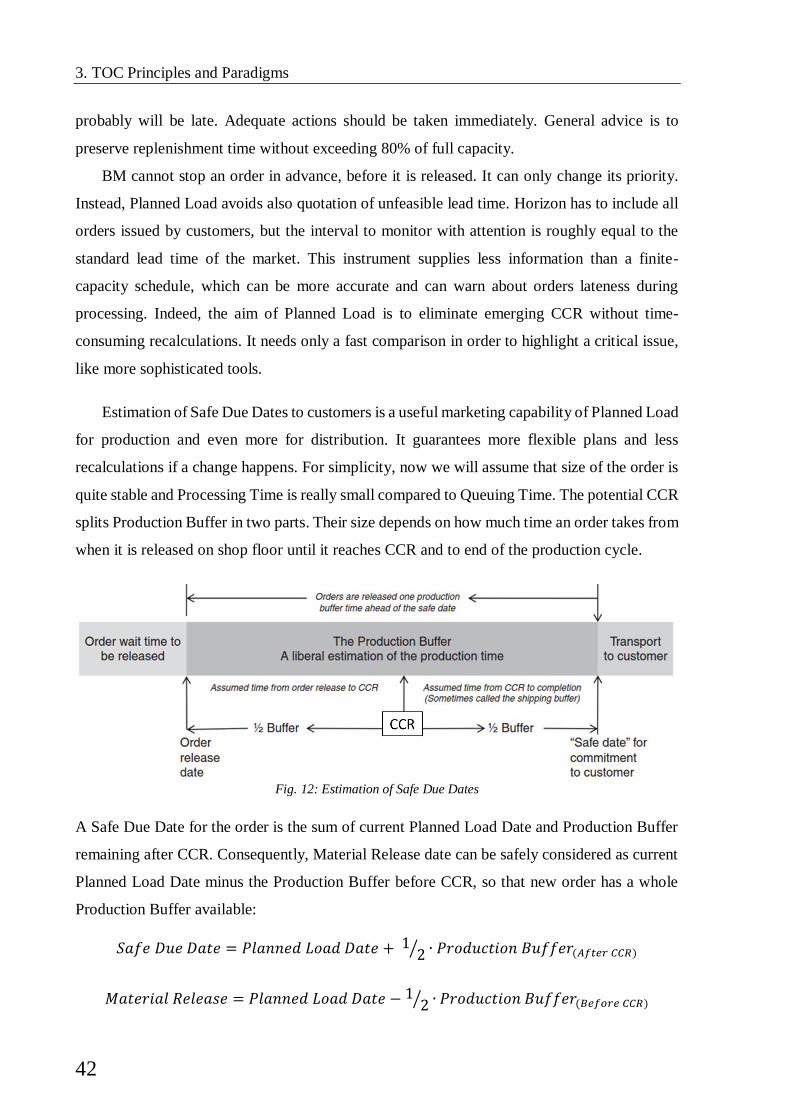
3. TOC Principles and Paradigms
42
probably will be late. Adequate actions should be taken immediately. General advice is to
preserve replenishment time without exceeding 80% of full capacity.
BM cannot stop an order in advance, before it is released. It can only change its priority.
Instead, Planned Load avoids also quotation of unfeasible lead time. Horizon has to include all
orders issued by customers, but the interval to monitor with attention is roughly equal to the
standard lead time of the market. This instrument supplies less information than a finite-
capacity schedule, which can be more accurate and can warn about orders lateness during
processing. Indeed, the aim of Planned Load is to eliminate emerging CCR without time-
consuming recalculations. It needs only a fast comparison in order to highlight a critical issue,
like more sophisticated tools.
Estimation of Safe Due Dates to customers is a useful marketing capability of Planned Load
for production and even more for distribution. It guarantees more flexible plans and less
recalculations if a change happens. For simplicity, now we will assume that size of the order is
quite stable and Processing Time is really small compared to Queuing Time. The potential CCR
splits Production Buffer in two parts. Their size depends on how much time an order takes from
when it is released on shop floor until it reaches CCR and to end of the production cycle.
A Safe Due Date for the order is the sum of current Planned Load Date and Production Buffer
remaining after CCR. Consequently, Material Release date can be safely considered as current
Planned Load Date minus the Production Buffer before CCR, so that new order has a whole
Production Buffer available:
𝑆𝑎𝑓𝑒 𝐷𝑢𝑒 𝐷𝑎𝑡𝑒 = 𝑃𝑙𝑎𝑛𝑛𝑒𝑑 𝐿𝑜𝑎𝑑 𝐷𝑎𝑡𝑒 + 12⁄ ∙ 𝑃𝑟𝑜𝑑𝑢𝑐𝑡𝑖𝑜𝑛 𝐵𝑢𝑓𝑓𝑒𝑟(𝐴𝑓𝑡𝑒𝑟 𝐶𝐶𝑅)
𝑀𝑎𝑡𝑒𝑟𝑖𝑎𝑙 𝑅𝑒𝑙𝑒𝑎𝑠𝑒 = 𝑃𝑙𝑎𝑛𝑛𝑒𝑑 𝐿𝑜𝑎𝑑 𝐷𝑎𝑡𝑒 − 12⁄ ∙ 𝑃𝑟𝑜𝑑𝑢𝑐𝑡𝑖𝑜𝑛 𝐵𝑢𝑓𝑓𝑒𝑟(𝐵𝑒𝑓𝑜𝑟𝑒 𝐶𝐶𝑅)
Fig. 12: Estimation of Safe Due Dates
3. TOC Principles and Paradigms
43
Generally, half of the Production Buffer is a recommended value whatever the position of the
potential CCR. This avoids problems during the first identification of CCR. Anyway, it can be
refined after identification of CCR position. Moreover, this interval should be sufficient for BM
to correct priorities and eventually to give precedence to late orders. This formulation is
preferable to a Production Buffer time ahead of the due date, as it is calculated in DBR. This
value avoids idle time at CCR. If Safe Due Date is shorter than the Standard Lead Time quoted
by the market also for new orders, then no critical situations are present at the time of calculation
of Planned Load. This is not a guarantee that received orders will be on time, because probably
they need to be processed from other resources after CCR. A strong limitation of Planned Load
is that it assumes all precedent due dates as given.
BM is the only control once an order is released. Its functioning is not different from DBR,
but it is more critical. Priorities have to be well defined because production is more flexible
than in S-DBR.
Differences between the two models are visible and tangible. S-DBR requires only
Shipping Buffer to be maintained. Assembly and Constraint Buffers are unnecessary without a
CCR. Shop floor control is simplified using directly Master Production Schedule and not CCR
schedule. This translates in a shorter lead time and higher responsiveness.
Implementation and control of S-DBR are surely easier than DBR, too. A complex situation
does not require more detailed schedules, but a simpler approach. S-DBR performs well in this
cases, while traditional DBR is not suited due to the calculation of many schedules. The same
goes for a system with multiple CCR or worse cases where they move along the system.
Stability of schedules is a critical point in traditional DBR. New or deleted orders affect Master
Production Schedule, which implies a probable recalculation of various schedules. This
problem is minimized (but not eliminated) in S-DBR because it is based on Master Production
Schedule. Also CCR schedules are subordinated to it. Moreover, S-DBR can anticipate capacity
problems with Planned Load.
3.5.2 - Make-To-Availability
TOC describes Make-To-Availability (MTA) as Make-To-Stock with a marketing message. It
commits to the perfect availability of an item at a specific location (Cox III et al., 2012).
MTA is definitely a subset of MTS, but it can grant a competitive edge if the commitment to
availability is correctly communicated to customers. In order to accomplish this, TOC modifies
furtherly DBR model and applies it to a MTS context. MTA is not a substitute of MTS. Make-
3. TOC Principles and Paradigms
44
to-stock is necessary in situations like producing in advance, levelling load before a demand
peak or when lead time requests by customer is shorter than Production Lead Time.
MTA is very near and similar to TOC Replenishment solution and can be considered its
precursor in a production environment. In a broad meaning also Vendor Managed Inventory
(VMI) is a type of MTA, where stock is at customer location.
Schragenheim highlights five points that guide the correct implementation of MTA
(Schragenheim et al., 2009):
1. Inventory and replenishment time are closely correlated.
2. Work-in-process supplements protection of availability.
3. Tomorrow will be similar to today.
4. Status of finished inventory dictates production floor priorities.
5. Stagnation is undesirable.
The first and second observations are just a reformulation of the “Little’s Law”. They point out
that if an increase in stock were to happen in order to maintain availability, then an equivalent
enlargement of Replenishment Time would be necessary. This operation of stock increment is
the corresponding of an elongation of Production Buffer in DBR if due dates are not met.
Buffers are evaluated using quantities instead of time, but they have the same purpose they had
in MTO. The meaning of Production Buffer is not changed; it is still a protection. The difference
is that in a context like MTA there are not explicit due dates, but commitment on availability.
It has to cope with the interval between the sale of an item and the arrival of the replenishment:
𝑃𝑟𝑜𝑑𝑢𝑐𝑡𝑖𝑜𝑛 𝐵𝑢𝑓𝑓𝑒𝑟 = 𝐹𝑖𝑛𝑖𝑠ℎ𝑒𝑑 𝐺𝑜𝑜𝑑𝑠 + 𝑊𝐼𝑃
WIP is a protection to availability, too. MTA imposes a limit to the value of Production Buffer,
given that both finished goods and what is in the pipeline assures availability. This limit is
called Target Level. Two simple methods are employed for the selection of initial Target
Levels: “Paranoia Factor” and “Reliable Replenishment Time”. The first method is simple, but
quite subjective and it is not safe in case of sequence-dependent setup; on the other hand, the
second approach is generally better, but it needs at least 6-12 months of data. These methods
are explained below, in paragraph dedicated to distribution.
The hypothesis of having day by day similar demand makes the system stable on the short
term, ensuring validity of Little’s Law. In absence of any evidence of changes, MTA will
continue to produce only what was consumed in the precedent period. Total quantity of stock

3. TOC Principles and Paradigms
45
does not change significantly. When a product is consumed, a production order is generated. In
this manner replenishment quantities are known, making it a pull system. They do not change
the overall level of stock. TOC avoids every form of long-term forecast with this assumption
and adapts the model to short-term characteristics of DBR. MTA is not interested in what is
sold on average in a period, but in what might be sold if a peak were to happen in that period.
Forecasts should try to individuate the maximum value of sales, not a probable mean.
Differently from a push MTS, order quantities are not just an estimation of consumption during
a certain period. It is different also from MTO, where they are precisely defined by customer
orders.
Deviations from the Target Level of each item define orders priorities. Orders are released
without any due date in MTA, so BM cannot establish priorities looking at Time Buffers. Lack
of due dates limits performance measurements concerning time in MTS. In fact, availability is
a better indicator. A system similar to BM assigns a priority to each order that is going to be
released in production. MTA adopts a modified version of Buffer Status. Priorities depends on
the quantity of stock positioned downstream the order, between its position and Production
Buffer:
𝐵𝑢𝑓𝑓𝑒𝑟 𝑆𝑡𝑎𝑡𝑢𝑠(%) =𝑂𝑛 𝐻𝑎𝑛𝑑 + 𝑃𝑖𝑝𝑒𝑙𝑖𝑛𝑒
𝑇𝑎𝑟𝑔𝑒𝑡 𝐿𝑒𝑣𝑒𝑙× 100
The division in three coloured zones provides a visual reference about urgency even before
releasing orders. The number of orders entering in shop floor is tied to the current value of
Planned Load, like in S-DBR.
The last guideline supports a new element of control system for MTA. It is an improvement
to Buffer Management, called Dynamic Buffer Management (DBM): an intervention is
necessary to resize Target Levels when too much orders are constantly in red or green zone.
This allows the system to get a new balance with a gradual adaptation and to avoid disruption
in the short-term. This mechanism will be explained extensively later, because it is central for
TOC Replenishment.
Two important premises before the adoption of the MTA solution should be noted. The
first is that initial Target Level set with the methods explain above is only temporary. Those
values are proxies before MTA is stabilized. They will be monitored and adapted by DBM in
order to face actual demand. The second is that finished goods buffer should be full since the
initial implementation of MTA, otherwise DBM could cause problems with wrong adjustments.

3. TOC Principles and Paradigms
46
The biggest risk for MTA is a growing market (Cox III & Schleier, 2010). In MTO is possible
to quote longer lead time in order to avoid an overwhelming demand, but MTA cannot do this.
It is in contrast with the principle of MTA itself. Capacity Management and the correct use of
Planned Load is a key element to maintain some idle capacity. Preserve a little more capacity
than what CCR is capable to handle is required.
Similar studies to this thesis have been already brought to the attention of researchers during
last decades, but most of them is concentrated on production side. These works are a start point,
providing ideas and methodology in a new field of research as distribution networks.
Comparisons of DBR with other scheduling systems are numerous. (Mabin & Gibson, 1998)
sustains the synergies with Linear Programming. (Chakravorty, 2001) examines performance
of DBR on shop floor comparing it with two workload control policies. Results highlight the
effectiveness of DBR if CCR is protected adequately with some extra capacity. (Steele et al.,
2005) perform a simulation supported by a real case of transition from MRP to DBR. Although
DBR surpasses MRP on the field, they modify MRP with a DBR-like policy that greatly
improves classic performance and argue the importance of a pull policy. A great number of
studies on Just-in-Time and DBR is available in literature, using any kind of simulation,
hypothesis and industry. (K. J. Watson & Patti, 2008) corroborates evidences that under the
same conditions JIT requires a greater quantity of inventory in order to achieve the same level
of output as DBR. They show a greater stability of DBR in presence of system variation.
A comprehensive review and a deeper analysis can be retrieved in (Gupta & Snyder, 2009).
They study literature that compares MRP, JIT and DBR. Their work argues the lack of empirical
and analytical articles and proposes a more methodical approach in future researches.
Nonetheless, they recognize that these researches bring interesting achievements that need to
be investigated with applications in real world. A new impulse to cases of study has been
launched following these suggestions. One of the most recent implementation is in (Darlington
et al., 2015), that show how TOC and DBR can perfectly complement Lean and Kanban.
47
4. TOC and Supply
Chain Management
Theory of Constraints philosophy aims to a systemic perspective in supply chain management.
Local optimizations are not effective, especially in contexts subject to high variability. Supply
chains are not always coordinated, so excess of stock and stockout are possible in the same
location as results of the “Forrester effect”.
4.1 - Supply Chain Replenishment System
The official TOCICO Dictionary (Cox III et al., 2012) defines TOC replenishment solution as:
Replenished stock usually is a quantity roughly equal to the actual sales of previous period. It
is based on the effective depletion of inventory. The most part of stock is held in a central
warehouse at the manufacturer. Only a small quantity is at regional warehouses (Schragenheim
et al., 2009). More frequent deliveries increase transportation cost, but this is more than
compensated by additional Throughput given by the high availability of items at retailers.
This definition is complied with six main decisions that help the shift from the former
replenishment system (Cox III & Schleier, 2010):
1) Aggregate stock at the highest level in the supply chain.
2) Determine stock buffer sizes for all chain locations based on demand, supply and
replenishment lead time.
3) Increase the frequency of replenishment.
4) Manage the flow of inventories using buffers and buffer penetration.
“A pull-distribution method that involves setting stock buffer sizes and then
monitoring and replenishing inventory within a supply chain based on the actual
consumption of the end user rather than a forecast. Each link in the supply chain
holds the maximum expected demand within the average replenishment time,
adjusted for the level of unreliability in replenishment time. Each link generally
receives what was shipped or sold, though this amount is adjusted up or down when
buffer management detects changes in the demand pattern”

4. TOC and Supply Chain Management
48
5) Use Dynamic Buffer Management (DBM).
6) Set manufacturing priorities according to urgency in stock buffers at Plant
Warehouse.
4.1.1 - Aggregate Stock
The principle behind TOC Supply Chain Replenishment System (SCRS) is the “Law of large
numbers”. Statistical fluctuations of supply and demand are sharply reduced aggregating stock
closest as possible to the source/plant. This is a result already known since the studies of Maister
on effects of stock centralisation and the so-called “Root Law” (Maister, 1976). Further
refinements on total cost reduction due to risk pooling were proposed by Eppen (Eppen, 1979).
The first step is identification of divergence points in supply chain. Tools like VAT analysis
can be useful to analyse the flow and find critical points where variety explodes or inventory is
excessive. Aggregation of inventory in these locations and establishing central warehouses
provides a notable reduction of variability. Plant Warehouses (PWH) and Central Warehouses
(CWH) replenish retailers keeping stock at acceptable levels. Indeed, the effect of this
aggregation is a reduction of stock level in the whole supply chain. These locations guarantee
the lowest level of inventory possible, as demonstrated. Their position is not always favourable
in order to meet Point of Sales (POS) requests. Other Regional Warehouses (RWH) would be
necessary closer to final consumption point if transportation time were excessive or lead times
were a strong qualifier to the market (Cox III & Schleier, 2010).
A change to distribution network is not required in a first implementation, SCRS can be adapted
to the actual structure. These are strategic considerations that are bound to Distribution Network
Design. They can be developed later, when also continuous improvement and other concepts
will be accepted.
4.1.2 - Determine Buffer
Buffers provide protection to Throughput. Their most important task is to secure it from every
disruption. Firstly, it is influenced by demand rate, supply and Replenishment Lead Time (RLT)
in a supply chain. Stock buffer size is connected directly to the level of safety desired and it
varies by item and location. As said for production, initial values of buffers size are not critical
decisions. They do not need a precise value to grant the success of implementation, because
DBM process will correct Target Level of each item driven by effective demand.
4. TOC and Supply Chain Management
49
TOC suggests two methods to determine initial buffers size, also adopted in production (Cox
III & Schleier, 2010):
Paranoia Factor: it consists in multiplying average demand rate during a certain period
and the corresponding Replenishment Time for a “Paranoia Factor”, usually 1.5 or 2, in
order to avoid peak of sales or blockage. This factor reflects the anxiety of a possible
stockout and adds a certain quantity of stock as additional safety.
Reliable Replenishment Time: it is called “reliable” because an order has a really high
probability (90%-95%) of arriving to destination within this time. It is different from
standard replenishment time, which is calculated on average. Reliable Replenishment
Time is greater than average and more similar to a maximum value. This method needs
historical time series of sales to evaluate the maximum peaks in the last year.
A good base for initial target value can be obtained using “Paranoia Factor” method, but it is
only a suggested cautious criterion to avoid a more complicated procedure.
Although demand and supply can be affected by actions of the firm, these imply external
interactions with market and supplier. TOC prefers controlling replenishment frequency in
order to influence Replenishment lead time. Its definition is slightly different from the
traditional one, deeply affecting system behaviour. APICS defines RLT as the “total period of
time that elapses from the moment it is determined that a product should be reordered until the
product is back on the shelf available for use” (Blackstone Jr., 2013). This definition refers to
the moment when the perception of need emerges. An order is placed only when it reaches
some type of trigger point that depends on the policy adopted. It can be a reorder level, a
minimum of stock or also a certain review frequency. RLT(TOC) is quite different because it
starts when an item is sold or consumed, so it includes the time that replenishment policy
requires to identify the need. RLT(TOC) comprises four different lead times:
𝑅𝐿𝑇(𝑇𝑂𝐶) = 𝑂𝑟𝑑𝑒𝑟𝐿𝑇 + 𝑃𝑟𝑒𝑟𝑒𝑙𝑒𝑎𝑠𝑒𝐿𝑇 + 𝑃𝑟𝑜𝑑𝑢𝑐𝑡𝑖𝑜𝑛𝐿𝑇 + 𝑇𝑟𝑎𝑛𝑠𝑝𝑜𝑟𝑡𝑎𝑡𝑖𝑜𝑛𝐿𝑇
Order LT: time from the consumption until a replenishment order is placed.
Prerelease LT: time between the acceptance of the order and its release to production.
Production LT: time from order release until it is ready for shipment or storing.
Transportation LT: time it takes to transport order to the point of sales/consumption.
An implementation of SCRS tries to reduce drastically replenishment lead time. The first
component of RLT is intrinsic in the replenishment model adopted. Monitoring frequencies and
4. TOC and Supply Chain Management
50
order points decide responsiveness of the system. Part of this component is not considered
explicitly by the APICS definition and it contributes to extend the risky interval with a non-
perfect availability. Improvements of Order LT are limited by economies of scale and also by
technologies, although nowadays this is no more a problem considering the advancements in
IT.
Prerelease and Production LT components are bounded to manufacturing environment.
Prerelease LT ends when rope signal is received by DBR or S-DBR and it is pulled in the
productive cycle. The ideal situation would be an instantaneous release into shop floor, but in
order to avoid overload a prerelease time is necessary. This lead time depends on actual load,
number of orders in queue and urgency. In a push system an order might be released to
production with less regard to the work in process. Pull solutions and capacity control can
provide a better reduction of Production LT. They grant also a continuous flow, with benefit on
capacity and Prerelease LT. S-DBR and Buffer Management are TOC pull solutions, but these
results are achievable following different ways, like Lean Production and Kanban.
The very limit of RLT is Transportation LT. The natural limit of RLT will be the distance and
transportation time between locations once a replenishment model, sufficient capacity and an
effective production cycle are in place.
4.1.3 - Increase Replenishment Frequency
Replenishment frequency is directly linked to responsiveness of the system. TOC tries to
unbalance the trade-off between inventory and transportation cost with the adoption of a new
set of measurements and a strong attention on availability instead of cost. Increased frequency
provides some benefits, like less amount of safety stock and more flexibility on shipments. TOC
suggests to increase the number of transportations, even more deliveries per day if necessary.
Improvements in Transportation LT are the most difficult to achieve. TOC suggests to exploit
them using faster transports, even if their cost is considerably higher. The higher transportation
costs are justified if studied with the measurements of Throughput Accounting. Cost of an
additional shipment is for the most part a TVC if the vehicle is owned. This cost is less than
marginal increment obtainable in Throughput in almost any case. The rationale is that
Throughput increment fully covers these additional costs. Moreover, inventory costs decrease
at the consumption points because stock is smaller for a shorter lead time. TOC recommends to
invest in variety when this happens, given that availability is at good level. Order LT is heavily

4. TOC and Supply Chain Management
51
reduced thanks to this replenishment model, because it delays an order for a shorter time before
the next shipment.
Batching orders to meet the right volume or benefit of big discounts are behaviour
discouraged by TOC. It suggests to create mixed orders so that all variety can be replenished
more frequently. Discounts from suppliers can be obtained in other way, like redefinition of
contracts regarding annual quantities, not single purchases.
4.1.4 - Manage Flow
Managing flow simply means to keep consistent buffers in every location of supply chain.
Number of buffers in a supply chain tends to explode with the enlargement of distribution
network. Different buffers for the same item are maintained in every location, even for slow-
moving articles. Small quantities scattered in various places are difficult to monitor and subject
to big oscillations. Aggregation at CWH achieves great results and makes controlling simpler.
SCRS uses Buffer Management as control mechanism. It monitors inventory level and
penetration with a measurement similar to Buffer Status, but considering buffer by unit of stock.
Buffer Status alone, as it is defined in
production, does not provide complete
information about stock in a distribution
network. Every local inventory is
associated to a specific Buffer Status
measurement. Hence, it provides only
partial data about a specific place and does
not consider supply chain as whole.
However, in supply chains there are stock along pipeline and some other in downstream
locations. A measure so location-dependent does not take in consideration precedent
replenishment actions and what is happening in other sites. Moreover, different buffers of a
same item are managed separately and not seen as connected.
This problem emerges when two or more orders from different locations are placed. Orders
priorities cannot be influenced only on Buffer Status at the stocking points. They could even
have a similar penetration or ignore a precedent replenishment. TOC defines Virtual Buffer
(VB) in order to coordinate items priorities in supply chain:
𝑉𝐵(%) =𝐴𝑔𝑔𝑟𝑒𝑔𝑎𝑡𝑒𝑑 𝑆𝑡𝑜𝑐𝑘(𝑃𝐼𝑃𝐸𝐿𝐼𝑁𝐸 + 𝐿𝑂𝐶𝐴𝐿)
𝑇𝑎𝑟𝑔𝑒𝑡 𝐿𝑒𝑣𝑒𝑙(𝐿𝑂𝐶𝐴𝐿)× 100
Fig. 13: Buffer Status

4. TOC and Supply Chain Management
52
It is calculated for every item, considering aggregated stock of what is on the pipeline, headed
to the next site, and stock already available locally. Stock varies with the closeness to the
customer, so a value of VB for an item is valid only until the next stocking point (Cox III &
Schleier, 2010). VB of an item is related to the local target level, but at the same time its urgency
reflects also precedent replenishment orders and all stock that is already on-hand.
Priorities are coordinated and changed dynamically with the same rules of buffer
management. They are defined by VB status in the next downstream location and not related to
the status of upstream inventory. They consider only what has been requested by point of sales.
Priorities of a same item are coordinated with the actual demand, providing full visibility on
the overall level of stock in the system.
Availability should take in account also stock in-transit, which is not yet arrived to destination.
It cannot be ignored as a form of protection. This measurement avoids replenishment
overreactions of the system. In fact, red zone will be reached locally in some sites, but VB can
monitor the overall level of stock. It highlights when this alarm needs interventions or if it has
been already replenished with a precedent order that is on the pipeline.
4.1.5 - Dynamic Buffer Management
TOC does not specify an optimal level for buffers and does not push necessarily towards an
inventory reduction. Dynamic Buffer Management (DBM) regulates buffers size on actual
demand and variations of the context. These adjustments are natural corrections of Buffer
Management mechanism, taking part in a finer tuning of its zones. Initial level of stock has an
impact only in early phase of a Buffer Management implementation, while the process is
warming up. When the process reaches a steady state, buffer size will be adjusted with DBM
algorithm as time goes. In a first time, buffers can be safely initialized on higher quantities in
order to avoid all disruptions. The above cited methods of Paranoia Factor and Reliable
Replenishment Time are of common use in SCRS applications. Their simplicity is suited for
the great number of buffers in a distribution network, proportional to number of items and
locations.
DBM modifies size of buffers under the condition of continuous high or low buffer
penetration. It works in reaction to actual level of inventory and has the advantage of being
responsive both to lowering and increasing in demand. When the irregular situation is stable for
a certain number of periods, it corrects the excess or shortage changing buffer size. DBM
identifies two categories of corrections:

4. TOC and Supply Chain Management
53
“Too much Green” (TMG): if buffer penetration is in green zone or above for a long
period. Size of buffer is excessive and inventory are accumulating, so DBM contrasts
overstocking with a reduction of buffer Target Level.
“Too much Red” (TMR): opposite to green. Here the risk is stockout, not overstocking.
DBM increases buffer size in order to stabilize buffer penetration in yellow zone.
A rule of common sense for BM and distribution is “report daily and transport frequently”
(Schragenheim et al., 2009). Longer intervals in placing orders requires more inventory, so a
check period of at least twice the replenishment time is considered conservative in order to
avoid TMG. If buffer is persistently in green zone for such a long time, then a reduction of its
size is necessary.
The opposite intervention is activated when a buffer remains regularly in red zone.
Replenishment is considered urgent following the rules of Buffer Management and it needs to
expedite orders immediately. Differently from TMG, entity of penetration is a relevant
information. It signals how much critical is situation.
Two algorithms are documented for identification of TMR in literature. The first is similar to
the mechanism applied in production and it is simply triggered by the amount of time on-hand
inventory remains below red level (Cox III & Schleier, 2010). The other one is more recent and
it is believed more effective, though it requires some more information. An increment of size
is recommended only if the cumulative sum of units below red zone during an interval equal to
replenishment time reaches the size of red zone itself (Schragenheim et al., 2009).
Finally, DBM does not operate if a steady state is achieved with a buffer penetration
between green and yellow zone. In this case Buffer Management is working correctly and
demand is pretty stable. Intervention of DBM is not even necessary in such a situation because
Fig. 14: Dynamic Buffer Management
4. TOC and Supply Chain Management
54
it could introduce an artificial disruption. Only minor corrections should be applied in order to
avoid stagnation. Further actions would be aimed at inventory reduction.
DBM adjusts stock level on contingency, so its corrections vary their intensity from item
to item. The suggested standard correction is a 33% increment/decrement of Target Level, but
it is influenced by importance of the product, strategic value of location where buffer is placed
and managerial decisions that support strong reactivity of DBM. These adjustments depend
entirely on the type of algorithm chosen. It can be a simple instruction as the suggested one or
taking in consideration other parameters. At the same manner, width of buffer zones is not an
unchangeable decision. DBM can adapt itself to greater complexity by working on simple rules
that control its functioning. However, these parameters can also be treated separately from
buffer size in more advanced applications. The key point is to study their penetrations
consistently with demand rate of the downstream sites.
A certain “cooling period” is required after every adjustment acted by DBM. The next
correction check should be delayed at least the time necessary for replenishment delivery to
reach the buffer, in order to stabilize it. Twice the replenishment time is the suggested value in
literature. It is more than conservative and avoids nervousness in adjustments.
This mechanism provides good results with gradual demand shifts, but it can introduce
some nervousness in case of sudden changes. DBM makes corrections very quickly and reacts
immediately to demand, but placement or removal of inventory are not instantaneous. This is
due to the natural adjustments of buffer level and to long transportation lead time. They cannot
be removed completely, but DBM can still be applied without worries if replenishment lead
time is not extremely long.
A similar problem is created by seasonality. If demand pattern assumes a steep and rapid
peak or a product is affected by strong seasonality, then DBM can support wrong or delayed
adjustments. In these cases, anticipation of demand is the only way to help a gradual shift
towards the peak. Seasonality could be caused by actions of the firm itself. Most common
explanations are promotions, an announced price adjustment or concentrated purchases at the
end of financial periods (for B2B firms). Nonetheless, if the reason of the disruptive events are
environmental variables, firms can only face them, being independent from their decisions.

4. TOC and Supply Chain Management
55
4.1.6 - Set Manufacturing Priorities
Five Focusing Steps are valid also in supply chain. Walker discusses the importance of the
correct identification of which partner in a supply chain should be the drum (Walker, 2002).
Subordination of a not CCR in production has a respective in a distribution network.
The problem is a coherent assignment of priorities with both production and distribution.
Urgency of an order should not be different between manufacturing and transportation,
otherwise it cannot flow smoothly through the system. Supply chain has to assume a point of
view that regards all actors and does not encourage local efficiency. VB is extended to
production in order to accomplish this, synchronizing S-DBR with the rest of the network. The
most reliable point for setting this mechanism is at the Plant Warehouse, which generally is the
highest level of aggregation. In this point VB can react to every variation in supply chain and
has a complete view on all downstream locations. If priority of production order depends on
VB, then it is influenced by all other stock remaining in the whole network, until the last emitted
order of the same item. This mechanism is not limited to shop floor, but includes orders from
all downstream locations.
4.2 - Local Performance Measurement
TOC supports global measurements, but they do not provide an immediate push to improvement
on local level. The three main measures are shifted on operative level:
(Simatupang et al., 2004) described how these measures should be used to manage supply chain
network performance. Reliability and effectiveness in each link of supply chain can be assessed
with Throughput-value-days (TVD) and Inventory-value-days (IVD). Suppliers can use IDV to
evaluate stock at retailer, while retailer can assess reliability of supplier using TDD. These
measures have not a correspondence in reality. They cannot be compared with other real
quantity, but only between them. Their sole purpose is to launch a clear signal and trigger
attention of the controller.
Local
level
Throughput-value-days TVD
Inventory-value-days IVD
Local Operating Expenses LOE
Table 9: Local Performance Measures
4. TOC and Supply Chain Management
56
(Schragenheim et al., 2009) reflected upon the usefulness of this measures when due date
performances are already close to 100%. A correct implementation of DBR leads to a marginal
role of these measures. Initial stages of model implementation or system with really high
variability can benefit of their value. However, it seems they are progressively made redundant.
(Gupta & Andersen, 2012) sustained the same conjecture and presented also a case where these
measurements push towards organizational changes. At the same time, they observed that
management seems to refuse this metrics because they have not a correspondence in reality.
Throughput-Value-Days
It is the potential Throughput generated by an order multiplied for the number of days late that
order accumulated before shipping. It is a measure of reliability of supply chain, an estimation
of the impact of late orders. The best achievement is to maintain this value to zero, because it
grows rapidly with every late order.
The assumption behind TVD is that customers have perception of damage and uncertainty the
more they wait. However, a correct value of this perception is not possible and every
measurement is unreliable. Taken this assumption, TOC tries to estimate the potential
improvement of the system. It shifts focus on supply chain itself. The losses suffered are safely
assumed higher than the value of throughput, so lost Throughput is seen as an opportunity cost.
The more an order has to wait before delivery, more it implies a deficiency of the system.
Inventory-Value-Days
IVD is computed as the sum of all current inventory on hand valued at the original purchase
price multiplied for the number of days since the inventory was received and it remains unsold.
It is a measure of effectiveness. Inventory should be set to the minimum required level in order
to maintain TVD at an acceptable level, ideally near zero. A growth of IVD value is sign of a
push behaviour and an accumulation of inventory not required. This metric is proven to be
effective at retailers and in levels of supply chain in direct contact with the market.
Local Operating Expense
It is equal to amount of operating expense that is directly under control of the local manager. It
is the least relevant between the three. Its purpose is to provide a simple measurement of
variations between real and planned expenses.
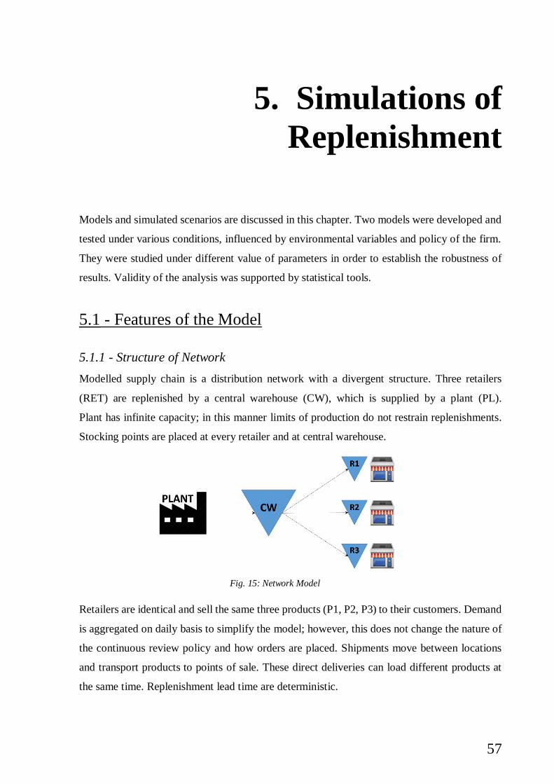
57
5. Simulations of
Replenishment
Models and simulated scenarios are discussed in this chapter. Two models were developed and
tested under various conditions, influenced by environmental variables and policy of the firm.
They were studied under different value of parameters in order to establish the robustness of
results. Validity of the analysis was supported by statistical tools.
5.1 - Features of the Model
5.1.1 - Structure of Network
Modelled supply chain is a distribution network with a divergent structure. Three retailers
(RET) are replenished by a central warehouse (CW), which is supplied by a plant (PL).
Plant has infinite capacity; in this manner limits of production do not restrain replenishments.
Stocking points are placed at every retailer and at central warehouse.
Retailers are identical and sell the same three products (P1, P2, P3) to their customers. Demand
is aggregated on daily basis to simplify the model; however, this does not change the nature of
the continuous review policy and how orders are placed. Shipments move between locations
and transport products to points of sale. These direct deliveries can load different products at
the same time. Replenishment lead time are deterministic.
Fig. 15: Network Model

5. Simulations of Replenishment
58
5.1.2 - Assumptions and Variables
Demand Generation
Simulations are conducted under stationary demand with low and high variability and then with
seasonality. The process of demand generation is slightly different.
Formula is based on that from (Chen, 2000a) and (Lee, 2000), but modified in order to introduce
a certain degree of instability. Original formula was:
𝐷𝑡 = 𝑘 + 𝜌 ∗ 𝐷𝑡−1 + 𝜀
𝐷𝑡 = Demand in period t
𝑘 = Not-negative constant
𝜌 = Correlation factor
𝜀 = White noise, Normal distribution N(0,1)
Demand generated by this formula is stable after a warm-up period. For great value of K, it is
almost flat and white noise is strongly reduced. Simulation of a greater variability is introduced
by using a Normal distribution with 𝜎2 ≠ 1 for the generation of white noise.
Without losing generality, it is modelled as:
𝐷𝑡 = 𝑚𝑎𝑥(𝑁(𝑘, 𝜎2) + 𝜌 ∗ 𝐷𝑡−1; 0)
This is nearly equivalent to the precedent for 𝜎2 = 1. It requires less calculation to the simulator
and, if necessary, can introduce a higher level of variability when it normally would reach
steady state. Also, high values of K do not limit variability and it oscillates around a certain
value at steady state.
Seasonality is introduced using a multiplicative component. Correlation is set to 0 in order
to avoid divergence and parameters of Normal is set with the values of steady state. It gradually
grows so that demand is two times the original value when it reaches its peak. Products do not
have peak at the same time, they are equally distributed along the year.
All simulations generate the same demand values thanks to the implementation of identical
seed generators in ARENA. This way, results are completely independent from random value,
though randomly generated.
𝑆1(𝑡) =1
2∗ sin (
2𝜋
300∗ 𝑡 +
𝜋
2) + 1.5
𝑆2(𝑡) =1
2∗ 𝑠𝑖𝑛 (
2𝜋
300∗ 𝑡 −
𝜋
6) + 1.5
𝑆3(𝑡) =1
2∗ 𝑠𝑖𝑛 (
2𝜋
300∗ 𝑡 −
5𝜋
6) + 1.5
NB: 300 days = 1 Year
5. Simulations of Replenishment
59
Stockout and Backorder
Stockout are recorded each time retailers or CW cannot meet demand. At retailers, every order
not entirely satisfied is recorded as a stockout. Available pieces are sold while the rest of the
order is considered lost. In this manner retailers cannot have backorders.
Indeed, backorders are allowed at Central Warehouse: available part of the order is delivered,
while the remaining is put in a queue until stock is replenished from plant. Stockout is recorded
in any case.
Ordering Costs
Demand is aggregated daily, so every day only one order for each product can be placed. Costs
under this category are:
- Costs of preparation and emission
- Administration costs
- Costs of receiving and control
- Transportation costs
The first three costs are considered as an aggregate in these models. Personnel in charge of
receiving and controlling goods at arrival of replenishments is not saturated, so accounting of
this cost is done for every order emission. Orders are placed independently for each product, so
a logic of joint replenishments optimization is not implemented.
Transportation costs are treated separately, paying a fee for every truck sent from supplier or
adopting a pay-per-use tariff.
Holding Costs
Typical components of this cost are listed here. Not all of them are considered in these models:
- Capital costs: interests on working capital or opportunity cost of the money
invested in the inventory.
- Storage costs: building and facility maintenance.
- Inventory Services costs: IT, personnel and physical handling of inventory,
Insurance and Taxes.
- Inventory Risk costs: damage, shrinkage, administrative errors, theft.
By hypothesis, they are set at 30 % for retailers and at 20% for central warehouse on annualized
basis (Creazza et al., 2010). Studies have reported that generally 5% - 15% are capital costs,
while the rest is split between the others (Richardson, 1995).
Products are considered not perishable, damageable or subject to theft; otherwise, inventory
risk is one of the most relevant cost in retail industry.
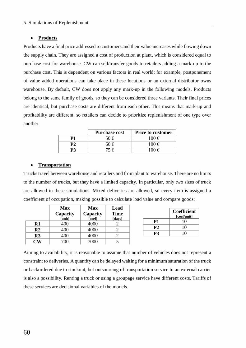
5. Simulations of Replenishment
60
Products
Products have a final price addressed to customers and their value increases while flowing down
the supply chain. They are assigned a cost of production at plant, which is considered equal to
purchase cost for warehouse. CW can sell/transfer goods to retailers adding a mark-up to the
purchase cost. This is dependent on various factors in real world; for example, postponement
of value added operations can take place in these locations or an external distributor owns
warehouse. By default, CW does not apply any mark-up in the following models. Products
belong to the same family of goods, so they can be considered three variants. Their final prices
are identical, but purchase costs are different from each other. This means that mark-up and
profitability are different, so retailers can decide to prioritize replenishment of one type over
another.
Purchase cost Price to customer
P1 50 € 100 €
P2 60 € 100 €
P3 75 € 100 €
Transportation
Trucks travel between warehouse and retailers and from plant to warehouse. There are no limits
to the number of trucks, but they have a limited capacity. In particular, only two sizes of truck
are allowed in these simulations. Mixed deliveries are allowed, so every item is assigned a
coefficient of occupation, making possible to calculate load value and compare goods:
Max
Capacity [unit]
Max
Capacity [coef]
Lead
Time [days]
R1 400 4000 2
R2 400 4000 2
R3 400 4000 2
CW 700 7000 5
Coefficient
[coef/unit]
P1 10
P2 10
P3 10
Aiming to availability, it is reasonable to assume that number of vehicles does not represent a
constraint to deliveries. A quantity can be delayed waiting for a minimum saturation of the truck
or backordered due to stockout, but outsourcing of transportation service to an external carrier
is also a possibility. Renting a truck or using a groupage service have different costs. Tariffs of
these services are decisional variables of the models.

5. Simulations of Replenishment
61
Loading Priorities
Mixed deliveries need a set of rules to define priorities between orders. Though capacity limit
of trucks can be overcome with multiple deliveries, goods are loaded with different priorities.
Deliveries with low priority or a low saturation can be avoided, but it is necessary a policy to
determine their status. Common policies consider either availability or profitability; DBM uses
a policy integrated with the rest of the methodology and based on Buffer Status.
All simulations are conducted aiming to full availability. In presence of order batching and
minimum saturation also mechanisms prioritizing the most profitable items are implemented.
Minimum Batch
Every product has a minimum order quantity to meet. This is an important limitation to the
effectiveness of replenishment policies if it is a constraint imposed by a supplier. ROP models
do not consider such a situation in these simulations, setting minimum order equal to EOQ.
Instead, this can be a policy constraint that greatly affects DBM, because order quantity is
supposed to adapt itself to demand. This is far from being an optimal reorder, but some batching
can improve cost performance of DBM without compromising it. By default, batch is set to 1
in the following DBM models, eliminating this effect.
Minimum Saturation
The same logic is applied to deliveries. Orders are loaded on one or more trucks; if an order
exceeds capacity limit of the vehicle, then a second truck is loaded. Naturally this imply to start
two deliveries and so an extra cost. Setting a minimum saturation partially avoids this situation,
stopping the second vehicle if it does not meet a requisite. A minimum saturation of truck
capacity has to be meet in order to start journey of a vehicle, otherwise the part of order
exceeding is backordered and has to wait until a sufficient load.
In this manner, the number of deliveries is reduced and a small cost optimization is done. An
internal policy can impose this limitation in real world, aiming to increase saturation of
deliveries.
5.1.3 - Recorded Parameters
Every replication records the same indexes for each product, both at retailers and CW. They are
collected in form of matrix 3x4 for simplicity, where the meaning of the first number is type of
goods (P1, P2, P3) and the other stays for the location (R1, R2, R3, CW): for example,
#Stockout(2,4) is the index for number of stockout of P2 at CW. The complete list of indicators:
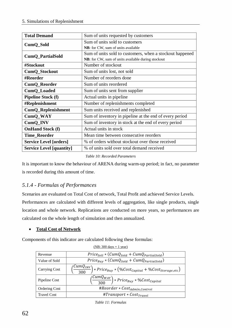
5. Simulations of Replenishment
62
Total Demand Sum of units requested by customers
CumQ_Sold Sum of units sold to customers
NB: for CW, sum of units available
CumQ_PartialSold Sum of units sold to customers, when a stockout happened
NB: for CW, sum of units available during stockout
#Stockout Number of stockout
CumQ_Stockout Sum of units lost, not sold
#Reorder Number of reorders done
CumQ_Reorder Sum of units reordered
CumQ_Loaded Sum of units sent from supplier
Pipeline Stock (f) Actual units in pipeline
#Replenishment Number of replenishments completed
CumQ_Replenishment Sum units received and replenished
CumQ_WAY Sum of inventory in pipeline at the end of every period
CumQ_INV Sum of inventory in stock at the end of every period
OnHand Stock (f) Actual units in stock
Time_Reorder Mean time between consecutive reorders
Service Level [orders] % of orders without stockout over those received
Service Level [quantity] % of units sold over total demand received
Table 10: Recorded Parameters
It is important to know the behaviour of ARENA during warm-up period; in fact, no parameter
is recorded during this amount of time.
5.1.4 - Formulas of Performances
Scenarios are evaluated on Total Cost of network, Total Profit and achieved Service Levels.
Performances are calculated with different levels of aggregation, like single products, single
location and whole network. Replications are conducted on more years, so performances are
calculated on the whole length of simulation and then annualized.
Total Cost of Network
Components of this indicator are calculated following these formulas:
(NB: 300 days = 1 year)
Revenue 𝑃𝑟𝑖𝑐𝑒𝑆𝑒𝑙𝑙 ∗ (𝐶𝑢𝑚𝑄𝑆𝑜𝑙𝑑 + 𝐶𝑢𝑚𝑄𝑃𝑎𝑟𝑡𝑖𝑎𝑙𝑆𝑜𝑙𝑑)
Value of Sold 𝑃𝑟𝑖𝑐𝑒𝐵𝑢𝑦 ∗ (𝐶𝑢𝑚𝑄𝑆𝑜𝑙𝑑 + 𝐶𝑢𝑚𝑄𝑃𝑎𝑟𝑡𝑖𝑎𝑙𝑆𝑜𝑙𝑑)
Carrying Cost (𝐶𝑢𝑚𝑄𝐼𝑁𝑉
300) ∗ 𝑃𝑟𝑖𝑐𝑒𝐵𝑢𝑦 ∗ (%𝐶𝑜𝑠𝑡𝐶𝑎𝑝𝑖𝑡𝑎𝑙 + %𝐶𝑜𝑠𝑡𝑆𝑡𝑜𝑟𝑎𝑔𝑒,𝑒𝑡𝑐)
Pipeline Cost (𝐶𝑢𝑚𝑄𝑊𝐴𝑌
300) ∗ 𝑃𝑟𝑖𝑐𝑒𝐵𝑢𝑦 ∗ %𝐶𝑜𝑠𝑡𝐶𝑎𝑝𝑖𝑡𝑎𝑙
Ordering Cost #𝑅𝑒𝑜𝑟𝑑𝑒𝑟 ∗ 𝐶𝑜𝑠𝑡𝐴𝑑𝑚𝑖𝑛,𝐶𝑜𝑛𝑡𝑟𝑜𝑙
Travel Cost #𝑇𝑟𝑎𝑛𝑠𝑝𝑜𝑟𝑡 ∗ 𝐶𝑜𝑠𝑡𝑇𝑟𝑎𝑣𝑒𝑙
Table 11: Formulas
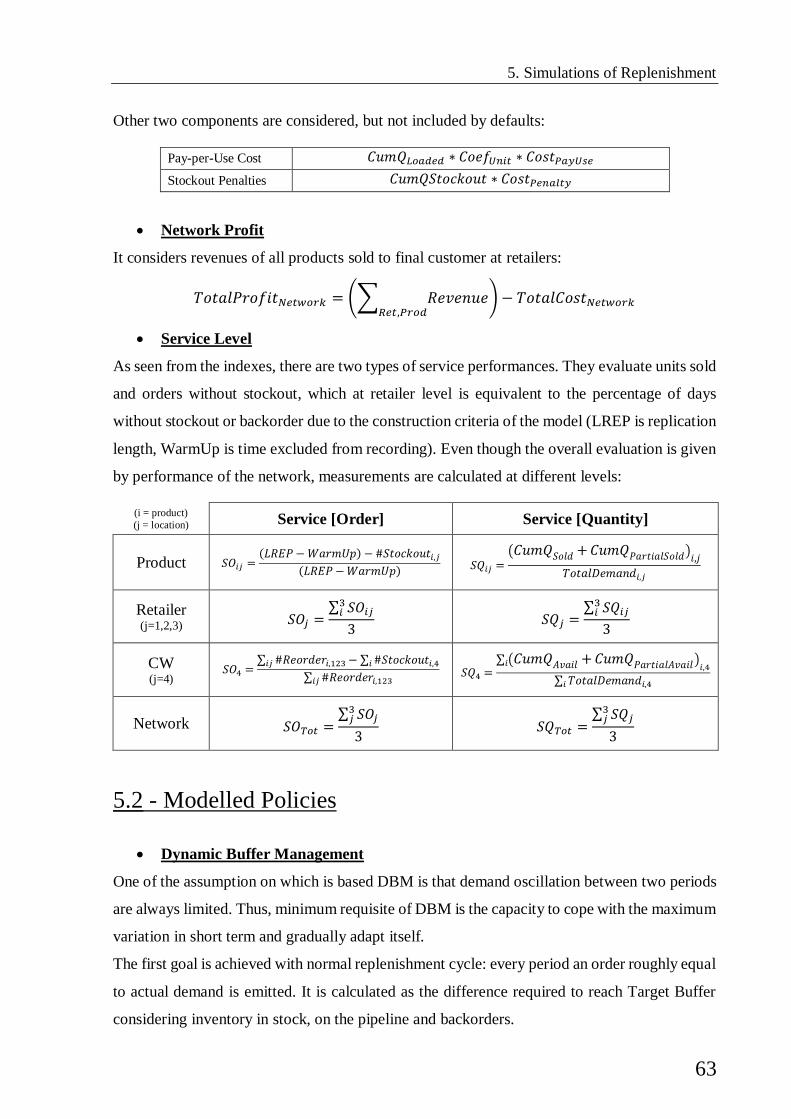
5. Simulations of Replenishment
63
Other two components are considered, but not included by defaults:
Pay-per-Use Cost 𝐶𝑢𝑚𝑄𝐿𝑜𝑎𝑑𝑒𝑑 ∗ 𝐶𝑜𝑒𝑓𝑈𝑛𝑖𝑡 ∗ 𝐶𝑜𝑠𝑡𝑃𝑎𝑦𝑈𝑠𝑒
Stockout Penalties 𝐶𝑢𝑚𝑄𝑆𝑡𝑜𝑐𝑘𝑜𝑢𝑡 ∗ 𝐶𝑜𝑠𝑡𝑃𝑒𝑛𝑎𝑙𝑡𝑦
Network Profit
It considers revenues of all products sold to final customer at retailers:
𝑇𝑜𝑡𝑎𝑙𝑃𝑟𝑜𝑓𝑖𝑡𝑁𝑒𝑡𝑤𝑜𝑟𝑘 = (∑ 𝑅𝑒𝑣𝑒𝑛𝑢𝑒𝑅𝑒𝑡,𝑃𝑟𝑜𝑑
) − 𝑇𝑜𝑡𝑎𝑙𝐶𝑜𝑠𝑡𝑁𝑒𝑡𝑤𝑜𝑟𝑘
Service Level
As seen from the indexes, there are two types of service performances. They evaluate units sold
and orders without stockout, which at retailer level is equivalent to the percentage of days
without stockout or backorder due to the construction criteria of the model (LREP is replication
length, WarmUp is time excluded from recording). Even though the overall evaluation is given
by performance of the network, measurements are calculated at different levels:
(i = product)
(j = location) Service [Order] Service [Quantity]
Product 𝑆𝑂𝑖𝑗 =(𝐿𝑅𝐸𝑃 − 𝑊𝑎𝑟𝑚𝑈𝑝) − #𝑆𝑡𝑜𝑐𝑘𝑜𝑢𝑡𝑖,𝑗
(𝐿𝑅𝐸𝑃 − 𝑊𝑎𝑟𝑚𝑈𝑝) 𝑆𝑄𝑖𝑗 =
(𝐶𝑢𝑚𝑄𝑆𝑜𝑙𝑑 + 𝐶𝑢𝑚𝑄𝑃𝑎𝑟𝑡𝑖𝑎𝑙𝑆𝑜𝑙𝑑)𝑖,𝑗
𝑇𝑜𝑡𝑎𝑙𝐷𝑒𝑚𝑎𝑛𝑑𝑖,𝑗
Retailer (j=1,2,3) 𝑆𝑂𝑗 =
∑ 𝑆𝑂𝑖𝑗3𝑖
3 𝑆𝑄𝑗 =
∑ 𝑆𝑄𝑖𝑗3𝑖
3
CW (j=4)
𝑆𝑂4 =∑ #𝑅𝑒𝑜𝑟𝑑𝑒𝑟𝑖,123𝑖𝑗 − ∑ #𝑆𝑡𝑜𝑐𝑘𝑜𝑢𝑡𝑖,4𝑖
∑ #𝑅𝑒𝑜𝑟𝑑𝑒𝑟𝑖,123𝑖𝑗 𝑆𝑄4 =
∑ (𝐶𝑢𝑚𝑄𝐴𝑣𝑎𝑖𝑙 + 𝐶𝑢𝑚𝑄𝑃𝑎𝑟𝑡𝑖𝑎𝑙𝐴𝑣𝑎𝑖𝑙)𝑖,4𝑖
∑ 𝑇𝑜𝑡𝑎𝑙𝐷𝑒𝑚𝑎𝑛𝑑𝑖,4𝑖
Network 𝑆𝑂𝑇𝑜𝑡 =∑ 𝑆𝑂𝑗
3𝑗
3 𝑆𝑄𝑇𝑜𝑡 =
∑ 𝑆𝑄𝑗3𝑗
3
5.2 - Modelled Policies
Dynamic Buffer Management
One of the assumption on which is based DBM is that demand oscillation between two periods
are always limited. Thus, minimum requisite of DBM is the capacity to cope with the maximum
variation in short term and gradually adapt itself.
The first goal is achieved with normal replenishment cycle: every period an order roughly equal
to actual demand is emitted. It is calculated as the difference required to reach Target Buffer
considering inventory in stock, on the pipeline and backorders.
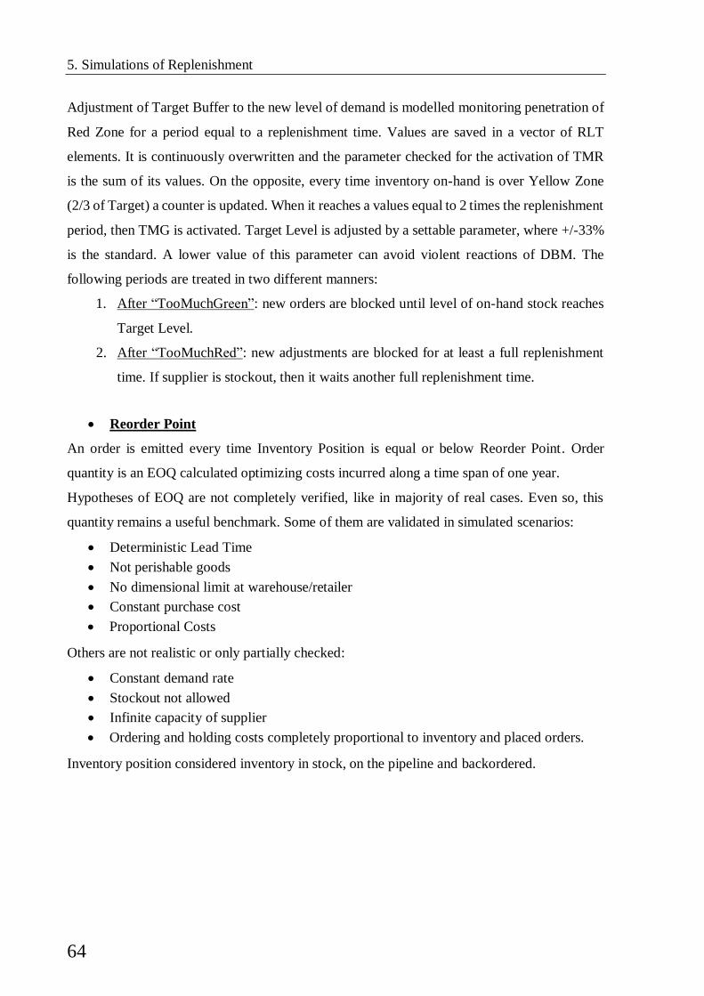
5. Simulations of Replenishment
64
Adjustment of Target Buffer to the new level of demand is modelled monitoring penetration of
Red Zone for a period equal to a replenishment time. Values are saved in a vector of RLT
elements. It is continuously overwritten and the parameter checked for the activation of TMR
is the sum of its values. On the opposite, every time inventory on-hand is over Yellow Zone
(2/3 of Target) a counter is updated. When it reaches a values equal to 2 times the replenishment
period, then TMG is activated. Target Level is adjusted by a settable parameter, where +/-33%
is the standard. A lower value of this parameter can avoid violent reactions of DBM. The
following periods are treated in two different manners:
1. After “TooMuchGreen”: new orders are blocked until level of on-hand stock reaches
Target Level.
2. After “TooMuchRed”: new adjustments are blocked for at least a full replenishment
time. If supplier is stockout, then it waits another full replenishment time.
Reorder Point
An order is emitted every time Inventory Position is equal or below Reorder Point. Order
quantity is an EOQ calculated optimizing costs incurred along a time span of one year.
Hypotheses of EOQ are not completely verified, like in majority of real cases. Even so, this
quantity remains a useful benchmark. Some of them are validated in simulated scenarios:
Deterministic Lead Time
Not perishable goods
No dimensional limit at warehouse/retailer
Constant purchase cost
Proportional Costs
Others are not realistic or only partially checked:
Constant demand rate
Stockout not allowed
Infinite capacity of supplier
Ordering and holding costs completely proportional to inventory and placed orders.
Inventory position considered inventory in stock, on the pipeline and backordered.
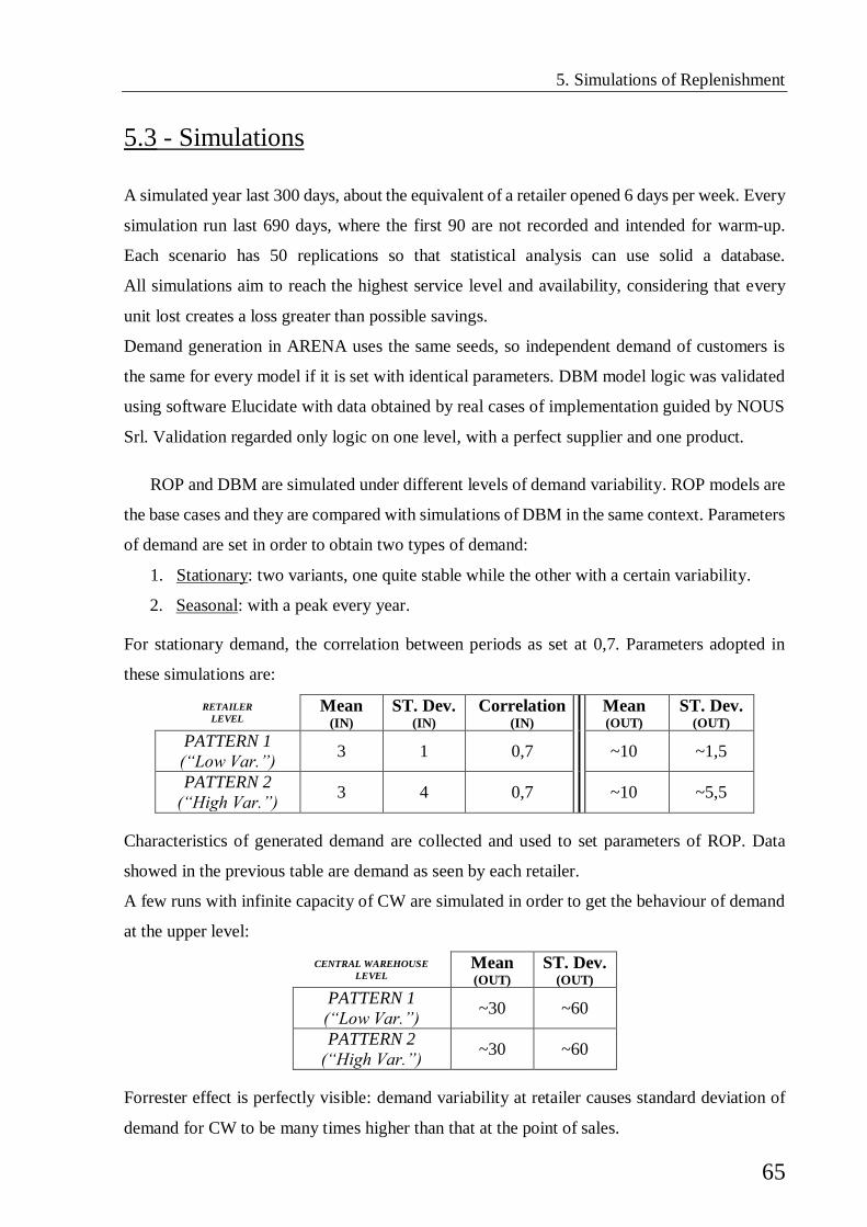
5. Simulations of Replenishment
65
5.3 - Simulations
A simulated year last 300 days, about the equivalent of a retailer opened 6 days per week. Every
simulation run last 690 days, where the first 90 are not recorded and intended for warm-up.
Each scenario has 50 replications so that statistical analysis can use solid a database.
All simulations aim to reach the highest service level and availability, considering that every
unit lost creates a loss greater than possible savings.
Demand generation in ARENA uses the same seeds, so independent demand of customers is
the same for every model if it is set with identical parameters. DBM model logic was validated
using software Elucidate with data obtained by real cases of implementation guided by NOUS
Srl. Validation regarded only logic on one level, with a perfect supplier and one product.
ROP and DBM are simulated under different levels of demand variability. ROP models are
the base cases and they are compared with simulations of DBM in the same context. Parameters
of demand are set in order to obtain two types of demand:
1. Stationary: two variants, one quite stable while the other with a certain variability.
2. Seasonal: with a peak every year.
For stationary demand, the correlation between periods as set at 0,7. Parameters adopted in
these simulations are:
RETAILER
LEVEL Mean
(IN) ST. Dev.
(IN) Correlation
(IN) Mean (OUT)
ST. Dev. (OUT)
PATTERN 1
(“Low Var.”) 3 1 0,7 ~10 ~1,5
PATTERN 2
(“High Var.”) 3 4 0,7 ~10 ~5,5
Characteristics of generated demand are collected and used to set parameters of ROP. Data
showed in the previous table are demand as seen by each retailer.
A few runs with infinite capacity of CW are simulated in order to get the behaviour of demand
at the upper level:
CENTRAL WAREHOUSE
LEVEL Mean (OUT)
ST. Dev. (OUT)
PATTERN 1
(“Low Var.”) ~30 ~60
PATTERN 2
(“High Var.”) ~30 ~60
Forrester effect is perfectly visible: demand variability at retailer causes standard deviation of
demand for CW to be many times higher than that at the point of sales.

5. Simulations of Replenishment
66
Initial targets of DBM are set using paranoia factor criteria, while initial stock is set at
slightly superior values both for ROP and DBM.
5.3.1 - Scenario 1: Stationary demand with low variability
Case 1: ROP
The following are the results using ROP with the first pattern. Uncertainty of demand is limited
so safety stock is very little in this simulation. As expected, it minimizes total costs providing
optimal results with stationary demand. Demand rate is almost constant so replenishments are
regular and transportation reduced. Levels of safety stock, reorder points and EOQ are
calculated with the standard formulas proposed in literature, imposing a service level of 97%:
NETWORK (n=50)
Mean
(�̅�)
ST. Dev. (𝝈)
Confidence
Interval (95%)
(±𝝈
√𝒏𝒕𝒏−𝟏,𝜶 𝟐⁄ )
Mean
(�̅�)
ST. Dev. (𝝈)
Confidence
Interval (95%)
(±𝝈
√𝒏𝒕𝒏−𝟏,𝜶 𝟐⁄ )
With tariff-per-unit With cost-per-vehicle
Profit € 974.261 4487 +/- € 1.275 € 964.078 4471 +/- € 1.271
Revenue € 2.702.639 11192 +/- € 3.181 = = =
Total Cost € 1.728.378 7019 +/- € 1995 € 1.738.561 7062 +/- € 2.007
Value of sold € 1.666.480 6971 +/- € 1.981 = = =
Carrying € 39.437 153,1 +/- € 43,5 = = =
Pipeline € 3.863 21,2 +/- € 6,03 = = =
Ordering € 828 5,44 +/- € 1,55 = = =
Transport € 17.770 121,3 +/- € 34,48 € 27.953 300,7 +/- € 85,5
Service [Ord] 99,95% 0,05% +/- 0,013% = = =
Service [Q] 99,97% 0,04% +/- 0,010% = = =
Table 12: ROP, low variability
Service level is nearly perfect, with average values over 99,9% in orders and quantities. These
tables report results of simulations in two manners, with a different treatment of transportation
costs: one pays a tariff per delivered unit, the other has a cost per sent vehicle. In the following
Graph 1: Scenario 1 - ROP, low variability

5. Simulations of Replenishment
67
paragraph will be explained the reasons of this choice. All comparisons will consider tariff-per-
unit from here on.
Previous outcome is the result of a loading priority based on urgency at the downstream
level. This criterion is similar to that proposed by DBM and is aimed to ensure availability.
Testing is conducted also prioritizing the most profitable items under a constraint of minimum
saturation:
NETWORK (n=50)
Mean
(�̅�)
Confidence
Interval (95%)
(±𝝈
√𝒏𝒕𝒏−𝟏,𝜶 𝟐⁄ )
Mean
(�̅�)
Confidence
Interval (95%)
(±𝝈
√𝒏𝒕𝒏−𝟏,𝜶 𝟐⁄ )
Mean
(�̅�)
Confidence
Interval (95%)
(±𝝈
√𝒏𝒕𝒏−𝟏,𝜶 𝟐⁄ )
Min 5% Sat. - Profit priority Min 10% Sat. - Profit priority Min 20% Sat. - Profit priority
Profit € 974.229 +/- € 1.273 € 973.706 +/- € 1.281 € 973.033 +/- € 1.315
Revenue € 2.702.503 +/- € 3.175 € 2.700.185 +/- € 3.199 € 2.697.159 +/- € 3.376
Total Cost € 1.728.274 +/- € 1.991 € 1.726.479 +/- € 2.006 € 1.724.126 +/- € 2.152
Value of sold € 1.666.384 +/- € 1.975 € 1.664.657 +/- € 1.993 € 1.662.419 +/- € 2.128
Carrying € 39.426 +/- € 43,48 € 39.350 +/- € 46,33 € 39.215 +/- € 48,42
Pipeline € 3.866 +/- € 6,10 € 3.887 +/- € 6,75 € 3.926 +/- € 8,85
Ordering € 828 +/- € 1,56 € 827 +/- € 1,50 € 826 +/- € 1,55
Transport € 17.771 +/- € 34,70 € 17.757 +/- € 32,25 € 17.740 +/- € 32,90
Service [Ord] 99,94% +/- 0,014% 99,85% +/- 0,025% 99,72% +/- 0,046%
Service [Q] 99,97% +/- 0,010% 99,88% +/- 0,023% 99,77% +/- 0,043%
Table 13: ROP, low var., minimum saturation and priority to profit
Low priority deliveries are avoided thanks to a minimum threshold. Saturation of vehicles
increases, but part of demand is lost due to this policy. It has an effect of cost reduction, but it
is counterbalanced by lost revenue. In these simulations the aim is availability. Setting loading
priorities on profitability has mainly drawbacks. It does not let deliveries to bring at retailers
what is really needed. Restraining the load to even higher minimum saturation deteriorates
performances even more.
Graph 2: Scenario 1 - Loading Priority to Profitability
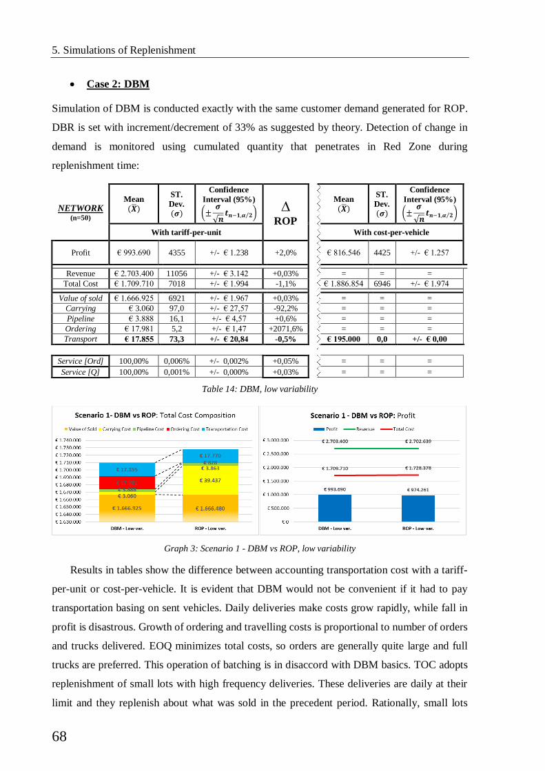
5. Simulations of Replenishment
68
Case 2: DBM
Simulation of DBM is conducted exactly with the same customer demand generated for ROP.
DBR is set with increment/decrement of 33% as suggested by theory. Detection of change in
demand is monitored using cumulated quantity that penetrates in Red Zone during
replenishment time:
NETWORK (n=50)
Mean
(�̅�)
ST.
Dev. (𝝈)
Confidence
Interval (95%)
(±𝝈
√𝒏𝒕𝒏−𝟏,𝜶 𝟐⁄ )
∆ ROP
Mean
(�̅�) ST.
Dev. (𝝈)
Confidence
Interval (95%)
(±𝝈
√𝒏𝒕𝒏−𝟏,𝜶 𝟐⁄ )
With tariff-per-unit With cost-per-vehicle
Profit € 993.690 4355 +/- € 1.238 +2,0%
€ 816.546 4425 +/- € 1.257
Revenue € 2.703.400 11056 +/- € 3.142 +0,03% = = =
Total Cost € 1.709.710 7018 +/- € 1.994 -1,1% € 1.886.854 6946 +/- € 1.974
Value of sold € 1.666.925 6921 +/- € 1.967 +0,03% = = =
Carrying € 3.060 97,0 +/- € 27,57 -92,2% = = =
Pipeline € 3.888 16,1 +/- € 4,57 +0,6% = = =
Ordering € 17.981 5,2 +/- € 1,47 +2071,6% = = =
Transport € 17.855 73,3 +/- € 20,84 -0,5% € 195.000 0,0 +/- € 0,00
Service [Ord] 100,00% 0,006% +/- 0,002% +0,05% = = =
Service [Q] 100,00% 0,001% +/- 0,000% +0,03% = = =
Table 14: DBM, low variability
Results in tables show the difference between accounting transportation cost with a tariff-
per-unit or cost-per-vehicle. It is evident that DBM would not be convenient if it had to pay
transportation basing on sent vehicles. Daily deliveries make costs grow rapidly, while fall in
profit is disastrous. Growth of ordering and travelling costs is proportional to number of orders
and trucks delivered. EOQ minimizes total costs, so orders are generally quite large and full
trucks are preferred. This operation of batching is in disaccord with DBM basics. TOC adopts
replenishment of small lots with high frequency deliveries. These deliveries are daily at their
limit and they replenish about what was sold in the precedent period. Rationally, small lots
Graph 3: Scenario 1 - DBM vs ROP, low variability
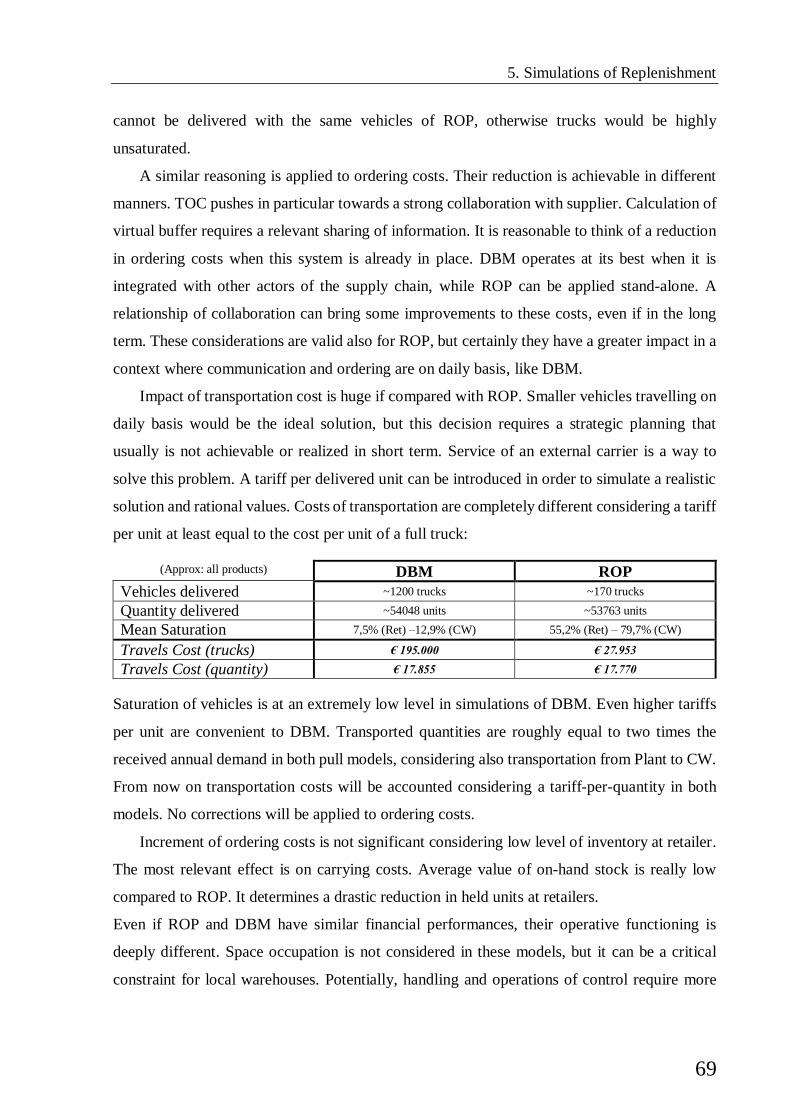
5. Simulations of Replenishment
69
cannot be delivered with the same vehicles of ROP, otherwise trucks would be highly
unsaturated.
A similar reasoning is applied to ordering costs. Their reduction is achievable in different
manners. TOC pushes in particular towards a strong collaboration with supplier. Calculation of
virtual buffer requires a relevant sharing of information. It is reasonable to think of a reduction
in ordering costs when this system is already in place. DBM operates at its best when it is
integrated with other actors of the supply chain, while ROP can be applied stand-alone. A
relationship of collaboration can bring some improvements to these costs, even if in the long
term. These considerations are valid also for ROP, but certainly they have a greater impact in a
context where communication and ordering are on daily basis, like DBM.
Impact of transportation cost is huge if compared with ROP. Smaller vehicles travelling on
daily basis would be the ideal solution, but this decision requires a strategic planning that
usually is not achievable or realized in short term. Service of an external carrier is a way to
solve this problem. A tariff per delivered unit can be introduced in order to simulate a realistic
solution and rational values. Costs of transportation are completely different considering a tariff
per unit at least equal to the cost per unit of a full truck:
(Approx: all products) DBM ROP
Vehicles delivered ~1200 trucks ~170 trucks
Quantity delivered ~54048 units ~53763 units
Mean Saturation 7,5% (Ret) –12,9% (CW) 55,2% (Ret) – 79,7% (CW)
Travels Cost (trucks) € 195.000 € 27.953
Travels Cost (quantity) € 17.855 € 17.770
Saturation of vehicles is at an extremely low level in simulations of DBM. Even higher tariffs
per unit are convenient to DBM. Transported quantities are roughly equal to two times the
received annual demand in both pull models, considering also transportation from Plant to CW.
From now on transportation costs will be accounted considering a tariff-per-quantity in both
models. No corrections will be applied to ordering costs.
Increment of ordering costs is not significant considering low level of inventory at retailer.
The most relevant effect is on carrying costs. Average value of on-hand stock is really low
compared to ROP. It determines a drastic reduction in held units at retailers.
Even if ROP and DBM have similar financial performances, their operative functioning is
deeply different. Space occupation is not considered in these models, but it can be a critical
constraint for local warehouses. Potentially, handling and operations of control require more
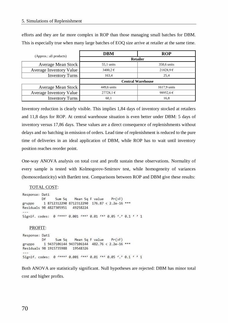
5. Simulations of Replenishment
70
efforts and they are far more complex in ROP than those managing small batches for DBM.
This is especially true when many large batches of EOQ size arrive at retailer at the same time.
(Approx.: all products) DBM ROP
Retailer
Average Mean Stock 55,1 units 358,6 units
Average Inventory Value 3400,2 € 21828,9 €
Inventory Turns 163,4 25,4
Central Warehouse
Average Mean Stock 449,6 units 1617,9 units
Average Inventory Value 27728,1 € 98952,6 €
Inventory Turns 60,1 16,8
Inventory reduction is clearly visible. This implies 1,84 days of inventory stocked at retailers
and 11,8 days for ROP. At central warehouse situation is even better under DBM: 5 days of
inventory versus 17,86 days. These values are a direct consequence of replenishments without
delays and no batching in emission of orders. Lead time of replenishment is reduced to the pure
time of deliveries in an ideal application of DBM, while ROP has to wait until inventory
position reaches reorder point.
One-way ANOVA analysis on total cost and profit sustain these observations. Normality of
every sample is tested with Kolmogorov-Smirnov test, while homogeneity of variances
(homoscedasticity) with Bartlett test. Comparisons between ROP and DBM give these results:
TOTAL COST:
PROFIT:
Both ANOVA are statistically significant. Null hypotheses are rejected: DBM has minor total
cost and higher profits.
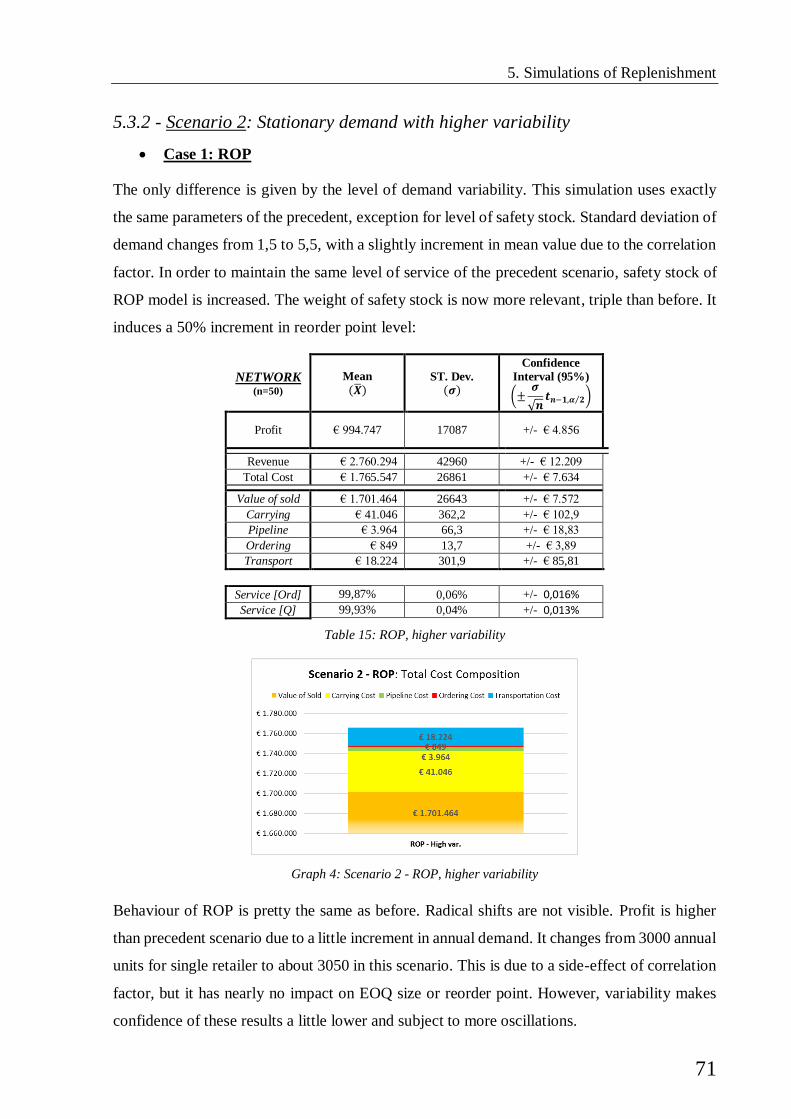
5. Simulations of Replenishment
71
5.3.2 - Scenario 2: Stationary demand with higher variability
Case 1: ROP
The only difference is given by the level of demand variability. This simulation uses exactly
the same parameters of the precedent, exception for level of safety stock. Standard deviation of
demand changes from 1,5 to 5,5, with a slightly increment in mean value due to the correlation
factor. In order to maintain the same level of service of the precedent scenario, safety stock of
ROP model is increased. The weight of safety stock is now more relevant, triple than before. It
induces a 50% increment in reorder point level:
NETWORK (n=50)
Mean
(�̅�)
ST. Dev. (𝝈)
Confidence
Interval (95%)
(±𝝈
√𝒏𝒕𝒏−𝟏,𝜶 𝟐⁄ )
Profit € 994.747 17087 +/- € 4.856
Revenue € 2.760.294 42960 +/- € 12.209
Total Cost € 1.765.547 26861 +/- € 7.634
Value of sold € 1.701.464 26643 +/- € 7.572
Carrying € 41.046 362,2 +/- € 102,9
Pipeline € 3.964 66,3 +/- € 18,83
Ordering € 849 13,7 +/- € 3,89
Transport € 18.224 301,9 +/- € 85,81
Service [Ord] 99,87% 0,06% +/- 0,016%
Service [Q] 99,93% 0,04% +/- 0,013%
Table 15: ROP, higher variability
Behaviour of ROP is pretty the same as before. Radical shifts are not visible. Profit is higher
than precedent scenario due to a little increment in annual demand. It changes from 3000 annual
units for single retailer to about 3050 in this scenario. This is due to a side-effect of correlation
factor, but it has nearly no impact on EOQ size or reorder point. However, variability makes
confidence of these results a little lower and subject to more oscillations.
Graph 4: Scenario 2 - ROP, higher variability

5. Simulations of Replenishment
72
Variability is covered by ROP with additional safety stock; nonetheless service levels show the
presence of a little number of not satisfied orders and that lost units increases. This drop of
service is infinitesimal. It does not impact customer perception nor performance of ROP.
It is important to note that setting of DBM is done in the most accurate possible way.
Results highlight how a correct regulation of parameters can stabilize performances also in
context with high variability.
This model is tested also giving higher loading priority to the most profitable items. The
results are similar to those with stable demand. A minimum saturation of 5% and priority to
profitable items have only marginal effects:
NETWORK (n=50)
Mean
(�̅�)
Confidence
Interval (95%)
(±𝝈
√𝒏𝒕𝒏−𝟏,𝜶 𝟐⁄ )
Mean
(�̅�)
Confidence
Interval (95%)
(±𝝈
√𝒏𝒕𝒏−𝟏,𝜶 𝟐⁄ )
Mean
(�̅�)
Confidence
Interval (95%)
(±𝝈
√𝒏𝒕𝒏−𝟏,𝜶 𝟐⁄ )
Min 5% Sat. - Profit priority Min 10% Sat. - Profit priority Min 20% Sat. - Profit priority
Profit € 994.701 +/- € 4.847 € 993.949 +/- € 4.852 € 993.200 +/- € 4.862
Revenue € 2.760.176 +/- € 12.178 € 2.757.162 +/- € 12.186 € 2.754.070 +/- € 12.204
Total Cost € 1.765.475 +/- € 7.612 € 1.763.213 +/- € 7.596 € 1.760.870 +/- € 7.613
Value of sold € 1.701.394 +/- € 7.552 € 1.699.212 +/- € 7.520 € 1.696.991 +/- € 7.544
Carrying € 41.042 +/- € 100,75 € 40.966 +/- € 91,99 € 40.828 +/- € 103,99
Pipeline € 3.966 +/- € 18,79 € 3.984 +/- € 19,12 € 4.017 +/- € 20,03
Ordering € 849 +/- € 3,85 € 848 +/- € 3,85 € 847 +/- € 3,98
Transport € 18.225 +/- € 85,18 € 18.204 +/- € 85,58 € 18.188 +/- € 88,88
Service [Ord] 99,86% +/- 0,017% 99,76% +/- 0,033% 99,65% +/- 0,043%
Service [Q] 99,92% +/- 0,014% 99,81% +/- 0,036% 99,70% +/- 0,046%
Table 16: ROP, higher var., minimum saturation and priority to profit
Graph 5: Scenario 2 - Loading Priority to Profitability
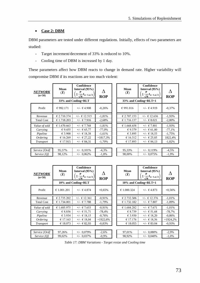
5. Simulations of Replenishment
73
Case 2: DBM
DBM parameters are tested under different regulations. Initially, effects of two parameters are
studied:
- Target increment/decrement of 33% is reduced to 10%.
- Cooling time of DBM is increased by 1 day.
These parameters affect how DBM reacts to change in demand rate. Higher variability will
compromise DBM if its reactions are too much violent:
NETWORK (n=50)
Mean
(�̅�)
Confidence
Interval (95%)
(±𝝈
√𝒏𝒕𝒏−𝟏,𝜶 𝟐⁄ )
∆ ROP
Mean
(�̅�)
Confidence
Interval (95%)
(±𝝈
√𝒏𝒕𝒏−𝟏,𝜶 𝟐⁄ )
∆ ROP
33% and Cooling=RLT 33% and Cooling=RLT+1
Profit € 992.171 +/- € 4.908 -0,26%
€ 991.016 +/- € 4.919 -0,37%
Revenue € 2.710.374 +/- € 12.515 -1,81% € 2.707.153 +/- € 12.636 -1,93%
Total Cost € 1.718.203 +/- € 7.916 -2,68% € 1.716.137 +/- € 8.021 -2,80%
Value of sold € 1.670.663 +/- € 7.768 -1,81% € 1.668.658 +/- € 7.881 -1,93%
Carrying € 9.455 +/- € 65,77 -77,0% € 9.379 +/- € 61,80 -77,1%
Pipeline € 3.900 +/- € 18,38 -1,61% € 3.895 +/- € 18,53 -1,75%
Ordering € 16.269 +/- € 27,22 +1817,3% € 16.312 +/- € 25,85 1822,4%
Transport € 17.915 +/- € 84,31 -1,70% € 17.893 +/- € 84,13 -1,82%
Service [Ord] 95,57% +/- 0,101% -4,3% 95,33% +/- 0,119% -4,5%
Service [Q] 98,12% +/- 0,062% -1,8% 98,00% +/- 0,075% -1,9%
NETWORK (n=50)
Mean
(�̅�)
Confidence
Interval (95%)
(±𝝈
√𝒏𝒕𝒏−𝟏,𝜶 𝟐⁄ )
∆ ROP
Mean
(�̅�)
Confidence
Interval (95%)
(±𝝈
√𝒏𝒕𝒏−𝟏,𝜶 𝟐⁄ )
∆ ROP
10% and Cooling=RLT 10% and Cooling=RLT+1
Profit € 1.001.201 +/- € 4.874 +0,65%
€ 1.000.324 +/- € 4.873 +0,56%
Revenue € 2.735.202 +/- € 12.361 -0,91% € 2.732.506 +/- € 12.376 -1,01%
Total Cost € 1.734.001 +/- € 7.788 -1,79% € 1.732.182 +/- € 7.807 -1,89%
Value of sold € 1.685.975 +/- € 7.653 -0,91% € 1.684.282 +/- € 7.671 -1,01%
Carrying € 8.856 +/- € 51,71 -78,4% € 8.739 +/- € 51,68 -78,7%
Pipeline € 3.934 +/- € 18,15 -0,76% € 3.930 +/- € 18,20 -0,86%
Ordering € 17.163 +/- € 18,04 +1922,6% € 17.176 +/- € 18,56 +1924,2%
Transport € 18.073 +/- € 82,93 -0,83% € 18.055 +/- € 83.04 -0,93%
Service [Ord] 97,26% +/- 0,079% -2,6% 97,01% +/- 0,080% -2,9%
Service [Q] 99,02% +/- 0,037% -0,9% 98,92% +/- 0,040% -1,0%
Table 17: DBM Variations - Target resize and Cooling time
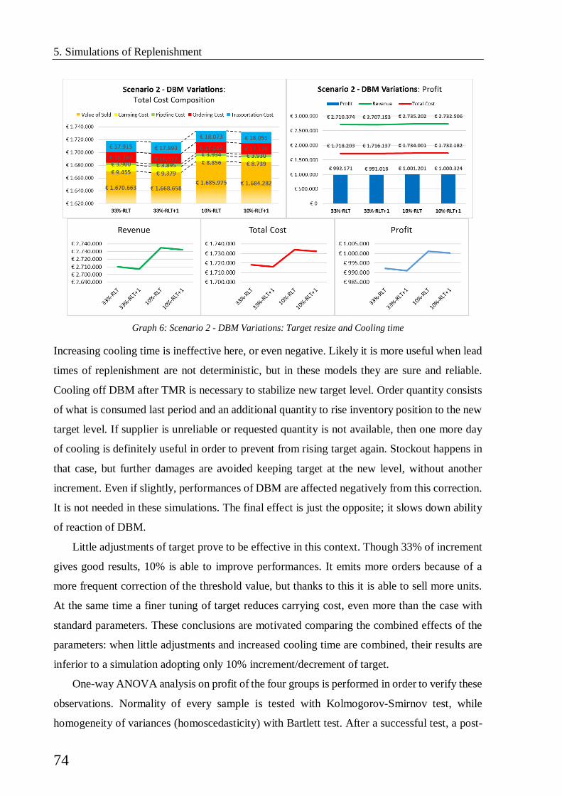
5. Simulations of Replenishment
74
Increasing cooling time is ineffective here, or even negative. Likely it is more useful when lead
times of replenishment are not deterministic, but in these models they are sure and reliable.
Cooling off DBM after TMR is necessary to stabilize new target level. Order quantity consists
of what is consumed last period and an additional quantity to rise inventory position to the new
target level. If supplier is unreliable or requested quantity is not available, then one more day
of cooling is definitely useful in order to prevent from rising target again. Stockout happens in
that case, but further damages are avoided keeping target at the new level, without another
increment. Even if slightly, performances of DBM are affected negatively from this correction.
It is not needed in these simulations. The final effect is just the opposite; it slows down ability
of reaction of DBM.
Little adjustments of target prove to be effective in this context. Though 33% of increment
gives good results, 10% is able to improve performances. It emits more orders because of a
more frequent correction of the threshold value, but thanks to this it is able to sell more units.
At the same time a finer tuning of target reduces carrying cost, even more than the case with
standard parameters. These conclusions are motivated comparing the combined effects of the
parameters: when little adjustments and increased cooling time are combined, their results are
inferior to a simulation adopting only 10% increment/decrement of target.
One-way ANOVA analysis on profit of the four groups is performed in order to verify these
observations. Normality of every sample is tested with Kolmogorov-Smirnov test, while
homogeneity of variances (homoscedasticity) with Bartlett test. After a successful test, a post-
Graph 6: Scenario 2 - DBM Variations: Target resize and Cooling time
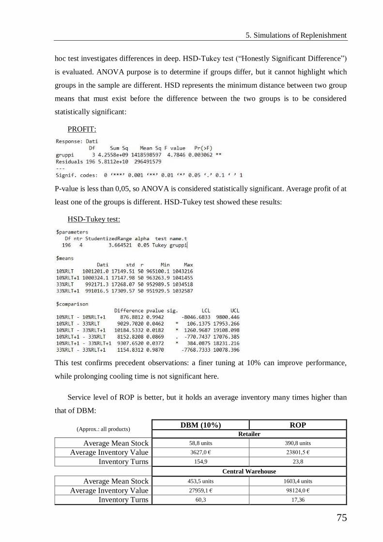
5. Simulations of Replenishment
75
hoc test investigates differences in deep. HSD-Tukey test (“Honestly Significant Difference”)
is evaluated. ANOVA purpose is to determine if groups differ, but it cannot highlight which
groups in the sample are different. HSD represents the minimum distance between two group
means that must exist before the difference between the two groups is to be considered
statistically significant:
PROFIT:
P-value is less than 0,05, so ANOVA is considered statistically significant. Average profit of at
least one of the groups is different. HSD-Tukey test showed these results:
HSD-Tukey test:
This test confirms precedent observations: a finer tuning at 10% can improve performance,
while prolonging cooling time is not significant here.
Service level of ROP is better, but it holds an average inventory many times higher than
that of DBM:
(Approx.: all products) DBM (10%) ROP Retailer
Average Mean Stock 58,8 units 390,8 units
Average Inventory Value 3627,0 € 23801,5 €
Inventory Turns 154,9 23,8
Central Warehouse
Average Mean Stock 453,5 units 1603,4 units
Average Inventory Value 27959,1 € 98124,0 €
Inventory Turns 60,3 17,36
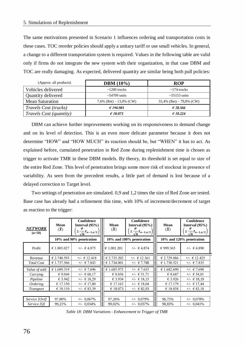
5. Simulations of Replenishment
76
The same motivations presented in Scenario 1 influences ordering and transportation costs in
these cases. TOC reorder policies should apply a unitary tariff or use small vehicles. In general,
a change to a different transportation system is required. Values in the following table are valid
only if firms do not integrate the new system with their organization, in that case DBM and
TOC are really damaging. As expected, delivered quantity are similar being both pull policies:
(Approx: all products) DBM (10%) ROP
Vehicles delivered ~1200 trucks ~174 trucks
Quantity delivered ~54709 units ~55153 units
Mean Saturation 7,6% (Ret) – 13,0% (CW) 55,4% (Ret) – 79,8% (CW)
Travels Cost (trucks) € 194.981 € 28.566
Travels Cost (quantity) € 18.073 € 18.224
DBM can achieve further improvements working on its responsiveness to demand change
and on its level of detection. This is an even more delicate parameter because it does not
determine “HOW” and “HOW MUCH” its reaction should be, but “WHEN” it has to act. As
explained before, cumulated penetration in Red Zone during replenishment time is chosen as
trigger to activate TMR in these DBM models. By theory, its threshold is set equal to size of
the entire Red Zone. This level of penetration brings some more risk of stockout in presence of
variability. As seen from the precedent results, a little part of demand is lost because of a
delayed correction to Target level.
Two settings of penetration are simulated. 0,9 and 1,2 times the size of Red Zone are tested.
Base case has already had a refinement this time, with 10% of increment/decrement of target
as reaction to the trigger:
NETWORK (n=50)
Mean
(�̅�)
Confidence
Interval (95%)
(±𝝈
√𝒏𝒕𝒏−𝟏,𝜶 𝟐⁄ )
Mean
(�̅�)
Confidence
Interval (95%)
(±𝝈
√𝒏𝒕𝒏−𝟏,𝜶 𝟐⁄ )
Mean
(�̅�)
Confidence
Interval (95%)
(±𝝈
√𝒏𝒕𝒏−𝟏,𝜶 𝟐⁄ )
10% and 90% penetration 10% and 100% penetration 10% and 120% penetration
Profit € 1.003.027 +/- € 4.875 € 1.001.201 +/- € 4.874 € 999.365 +/- € 4.890
Revenue € 2.740.593 +/- € 12.418 € 2.735.202 +/- € 12.361 € 2.729.886 +/- € 12.425
Total Cost € 1.737.566 +/- € 7.843 € 1.734.001 +/- € 7.788 € 1.730.521 +/- € 7.835
Value of sold € 1.689.319 +/- € 7.696 € 1.685.975 +/- € 7.653 € 1.682.690 +/- € 7.698
Carrying € 9.044 +/- € 60,17 € 8.856 +/- € 51,71 € 8.687 +/- € 54,01
Pipeline € 3.942 +/- € 18,29 € 3.934 +/- € 18,15 € 3.926 +/- € 18,19
Ordering € 17.150 +/- € 17,80 € 17.163 +/- € 18,04 € 17.179 +/- € 17,44
Transport € 18.110 +/- € 83,39 € 18.073 +/- € 82,93 € 18.038 +/- € 83,18
Service [Ord] 97,80% +/- 0,067% 97,26% +/- 0,079% 96,75% +/- 0,078%
Service [Q] 99,21% +/- 0,034% 99,02% +/- 0,037% 98,83% +/- 0,041%
Table 18: DBM Variations - Enhancement to Trigger of TMR
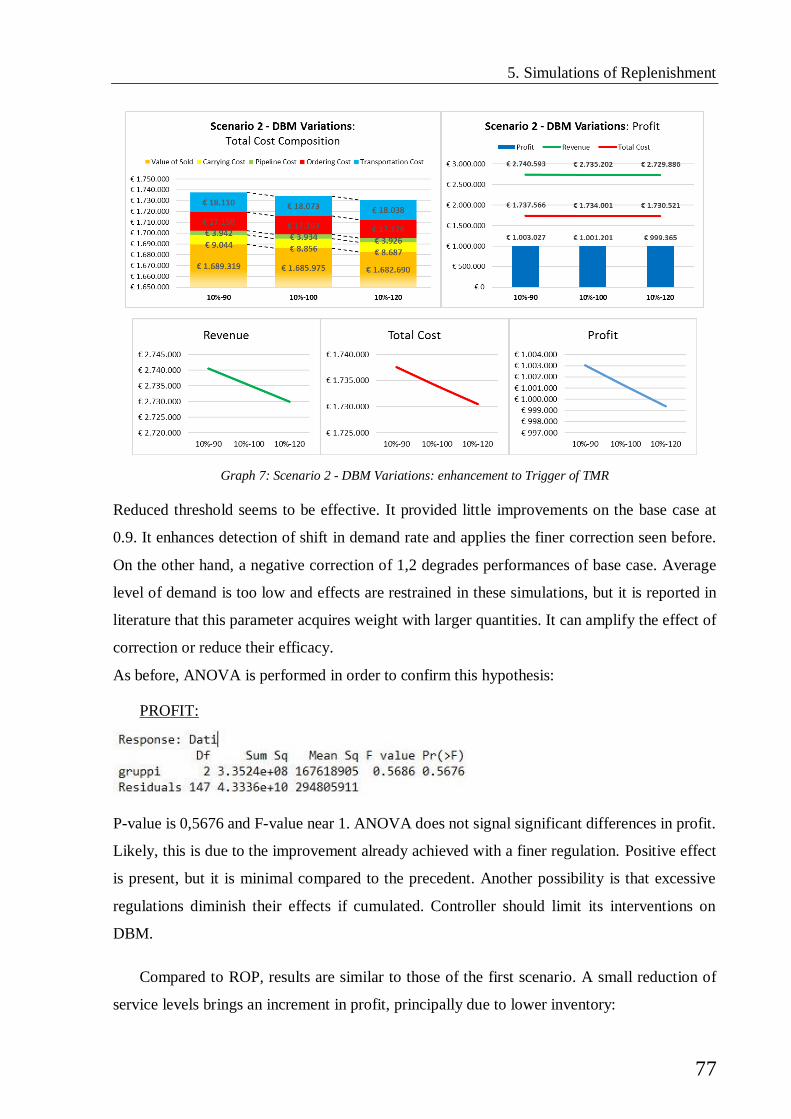
5. Simulations of Replenishment
77
Reduced threshold seems to be effective. It provided little improvements on the base case at
0.9. It enhances detection of shift in demand rate and applies the finer correction seen before.
On the other hand, a negative correction of 1,2 degrades performances of base case. Average
level of demand is too low and effects are restrained in these simulations, but it is reported in
literature that this parameter acquires weight with larger quantities. It can amplify the effect of
correction or reduce their efficacy.
As before, ANOVA is performed in order to confirm this hypothesis:
PROFIT:
P-value is 0,5676 and F-value near 1. ANOVA does not signal significant differences in profit.
Likely, this is due to the improvement already achieved with a finer regulation. Positive effect
is present, but it is minimal compared to the precedent. Another possibility is that excessive
regulations diminish their effects if cumulated. Controller should limit its interventions on
DBM.
Compared to ROP, results are similar to those of the first scenario. A small reduction of
service levels brings an increment in profit, principally due to lower inventory:
Graph 7: Scenario 2 - DBM Variations: enhancement to Trigger of TMR

5. Simulations of Replenishment
78
NETWORK (n=50)
10% and 90%
penetration ROP
∆ ROP
Profit € 1.003.027 € 994.747
+0,83%
Revenue € 2.740.593 € 2.760.294 -0,71%
Total Cost € 1.737.566 € 1.765.547 -1,58%
Value of sold € 1.689.319 € 1.701.464 -0,71%
Carrying € 9.044 € 41.046 -78,0%
Pipeline € 3.942 € 3.964 -0,6%
Ordering € 17.150 € 849 +1921,1%
Transport € 18.110 € 18.224 -0,63%
Service [Ord] 97,80% 99,87% -2,1%
Service [Q] 99,21% 99,93% -0,7%
Table 19: DBM vs ROP - Target Resize 10% and Trigger TMR 90%
ANOVA confirms the improvements:
TOTAL COST:
PROFIT:
Both ANOVA are statistically significant. However, ANOVA on profit highlights how
difference on this performance is less evident. DBM has better results on cost performances
than ROP, but they are very similar on overall profit.
Graph 8: Scenario 2 - DBM vs ROP: Target resize 10% and Trigger TMR 90%

5. Simulations of Replenishment
79
Order batching is another typical solution to cope with variability. Ordered quantities
become more regular reducing order frequency. Doing so, replenishments are normalized when
demand is really unstable. This is not the favourite solution for TOC; nonetheless, it is
mandatory in presence of a constraint on minimum order quantity from supplier. It is also
rational in case of unsaturated vehicles. Changing batch size gives the following results in this
simulation:
NETWORK (n=50)
(33% and
Cooling=RLT)
Mean
(�̅�)
Mean
(�̅�)
Mean
(�̅�)
Mean
(�̅�)
Mean
(�̅�)
Batch=None Batch=5 Batch=10 Batch=15 Batch=20
Profit € 992.171 € 994.142 € 996.100 € 990.765 € 988.542
Revenue € 2.710.374 € 2.712.686 € 2.712.130 € 2.690.901 € 2.681.228
Total Cost € 1.718.203 € 1.718.544 € 1.716.030 € 1.700.136 € 1.692.686
Value of sold € 1.670.663 € 1.672.007 € 1.671.776 € 1.658.662 € 1.652.744
Carrying € 9.455 € 9.486 € 9.582 € 9.802 € 10.124
Pipeline € 3.900 € 3.903 € 3.902 € 3.872 € 3.857
Ordering € 16.269 € 15.219 € 12.842 € 10.014 € 8.241
Transport € 17.915 € 17.930 € 17.927 € 17.786 € 17.721
Service [Ord] 95,57% 95,75% 96,29% 95,72% 95,31%
Service [Q] 98,12% 98,20% 98,18% 97,41% 97,06%
Table 20: DBM - Order Batching
Order batching improves ordering costs. A batch size approximately equal to daily demand
increases revenue and profit, with marginal effects on service levels. Larger batches are
Graph 9: Scenario 2 - DBM with batch
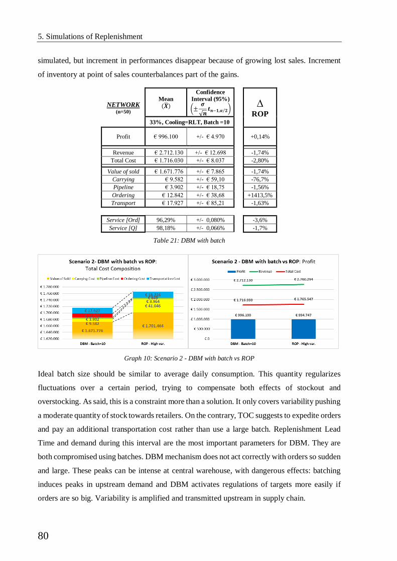
5. Simulations of Replenishment
80
simulated, but increment in performances disappear because of growing lost sales. Increment
of inventory at point of sales counterbalances part of the gains.
NETWORK (n=50)
Mean
(�̅�)
Confidence
Interval (95%)
(±𝝈
√𝒏𝒕𝒏−𝟏,𝜶 𝟐⁄ )
∆ ROP
33%, Cooling=RLT, Batch =10
Profit € 996.100 +/- € 4.970
+0,14%
Revenue € 2.712.130 +/- € 12.698 -1,74%
Total Cost € 1.716.030 +/- € 8.037 -2,80%
Value of sold € 1.671.776 +/- € 7.865 -1,74%
Carrying € 9.582 +/- € 59,10 -76,7%
Pipeline € 3.902 +/- € 18,75 -1,56%
Ordering € 12.842 +/- € 38,68 +1413,5%
Transport € 17.927 +/- € 85,21 -1,63%
Service [Ord] 96,29% +/- 0,080% -3,6%
Service [Q] 98,18% +/- 0,066% -1,7%
Table 21: DBM with batch
Ideal batch size should be similar to average daily consumption. This quantity regularizes
fluctuations over a certain period, trying to compensate both effects of stockout and
overstocking. As said, this is a constraint more than a solution. It only covers variability pushing
a moderate quantity of stock towards retailers. On the contrary, TOC suggests to expedite orders
and pay an additional transportation cost rather than use a large batch. Replenishment Lead
Time and demand during this interval are the most important parameters for DBM. They are
both compromised using batches. DBM mechanism does not act correctly with orders so sudden
and large. These peaks can be intense at central warehouse, with dangerous effects: batching
induces peaks in upstream demand and DBM activates regulations of targets more easily if
orders are so big. Variability is amplified and transmitted upstream in supply chain.
Graph 10: Scenario 2 - DBM with batch vs ROP

5. Simulations of Replenishment
81
5.3.3 - Scenario 3: Demand with seasonality
Case 1: ROP
Demand has seasonal peaks in this scenario. It grows gradually until it reaches two times the
regular level. Pattern is known, so demand rate is set at appropriate value for calculation of the
parameters of ROP:
NETWORK (n=50)
Mean
(�̅�)
ST. Dev. (𝝈)
Confidence
Interval (95%)
(±𝝈
√𝒏𝒕𝒏−𝟏,𝜶 𝟐⁄ )
Profit € 1.469.421 3218 +/- € 914
Revenue € 4.050.288 8132 +/- € 2.311
Total Cost € 2.580.867 5104 +/- € 1.450
Value of sold € 2.497.636 5083 +/- € 1.445
Carrying € 49.684 110,0 +/- € 31,27
Pipeline € 5.812 17,4 +/- € 4,95
Ordering € 1.033 4,8 +/- € 1,38
Transport € 26.703 121,8 +/- € 34,62
Service [Ord] 99,93% 0,043% +/- 0,012%
Service [Q] 99,96% 0,034% +/- 0,010%
Table 22: ROP, seasonality
Performances of ROP do not deteriorate. Peaks are gradual so it is able to cope with the change
in demand. Correct level of demand is monitored during warm-up period of the model. This is
possible in reality if historical series are available. Parameters of ROP are set in order to make
it performs the best availability. Seasonality increases variability of annual demand and risks
of shortage, so safety stock level is higher.
Graph 11: Scenario 3 - ROP, seasonality
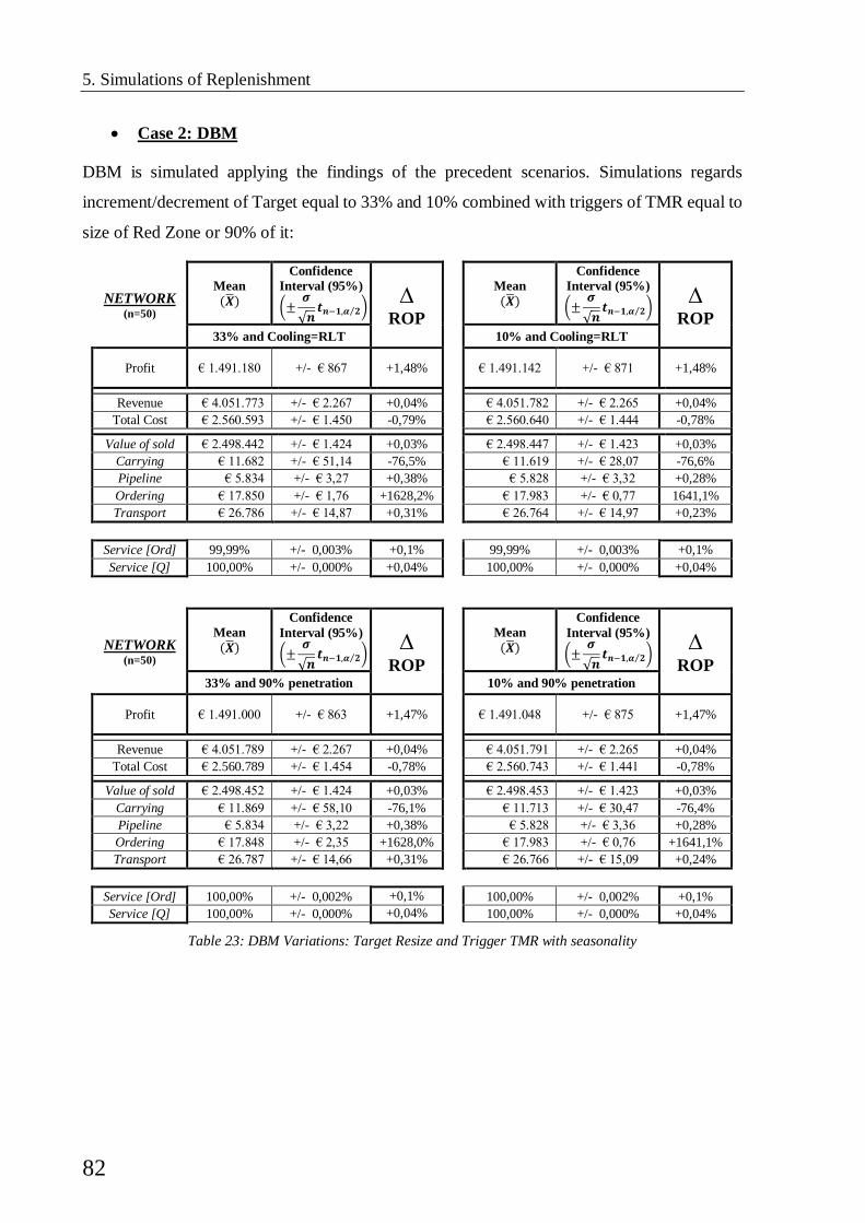
5. Simulations of Replenishment
82
Case 2: DBM
DBM is simulated applying the findings of the precedent scenarios. Simulations regards
increment/decrement of Target equal to 33% and 10% combined with triggers of TMR equal to
size of Red Zone or 90% of it:
NETWORK (n=50)
Mean
(�̅�)
Confidence
Interval (95%)
(±𝝈
√𝒏𝒕𝒏−𝟏,𝜶 𝟐⁄ )
∆ ROP
Mean
(�̅�)
Confidence
Interval (95%)
(±𝝈
√𝒏𝒕𝒏−𝟏,𝜶 𝟐⁄ )
∆ ROP
33% and Cooling=RLT 10% and Cooling=RLT
Profit € 1.491.180 +/- € 867 +1,48%
€ 1.491.142 +/- € 871 +1,48%
Revenue € 4.051.773 +/- € 2.267 +0,04% € 4.051.782 +/- € 2.265 +0,04%
Total Cost € 2.560.593 +/- € 1.450 -0,79% € 2.560.640 +/- € 1.444 -0,78%
Value of sold € 2.498.442 +/- € 1.424 +0,03% € 2.498.447 +/- € 1.423 +0,03%
Carrying € 11.682 +/- € 51,14 -76,5% € 11.619 +/- € 28,07 -76,6%
Pipeline € 5.834 +/- € 3,27 +0,38% € 5.828 +/- € 3,32 +0,28%
Ordering € 17.850 +/- € 1,76 +1628,2% € 17.983 +/- € 0,77 1641,1%
Transport € 26.786 +/- € 14,87 +0,31% € 26.764 +/- € 14,97 +0,23%
Service [Ord] 99,99% +/- 0,003% +0,1% 99,99% +/- 0,003% +0,1%
Service [Q] 100,00% +/- 0,000% +0,04% 100,00% +/- 0,000% +0,04%
NETWORK (n=50)
Mean
(�̅�)
Confidence
Interval (95%)
(±𝝈
√𝒏𝒕𝒏−𝟏,𝜶 𝟐⁄ )
∆ ROP
Mean
(�̅�)
Confidence
Interval (95%)
(±𝝈
√𝒏𝒕𝒏−𝟏,𝜶 𝟐⁄ )
∆ ROP
33% and 90% penetration 10% and 90% penetration
Profit € 1.491.000 +/- € 863 +1,47%
€ 1.491.048 +/- € 875 +1,47%
Revenue € 4.051.789 +/- € 2.267 +0,04% € 4.051.791 +/- € 2.265 +0,04%
Total Cost € 2.560.789 +/- € 1.454 -0,78% € 2.560.743 +/- € 1.441 -0,78%
Value of sold € 2.498.452 +/- € 1.424 +0,03% € 2.498.453 +/- € 1.423 +0,03%
Carrying € 11.869 +/- € 58,10 -76,1% € 11.713 +/- € 30,47 -76,4%
Pipeline € 5.834 +/- € 3,22 +0,38% € 5.828 +/- € 3,36 +0,28%
Ordering € 17.848 +/- € 2,35 +1628,0% € 17.983 +/- € 0,76 +1641,1%
Transport € 26.787 +/- € 14,66 +0,31% € 26.766 +/- € 15,09 +0,24%
Service [Ord] 100,00% +/- 0,002% +0,1% 100,00% +/- 0,002% +0,1%
Service [Q] 100,00% +/- 0,000% +0,04% 100,00% +/- 0,000% +0,04%
Table 23: DBM Variations: Target Resize and Trigger TMR with seasonality
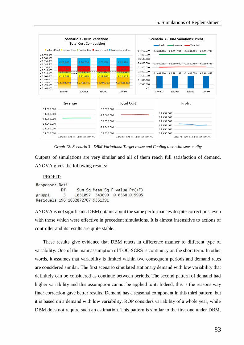
5. Simulations of Replenishment
83
Outputs of simulations are very similar and all of them reach full satisfaction of demand.
ANOVA gives the following results:
PROFIT:
ANOVA is not significant. DBM obtains about the same performances despite corrections, even
with those which were effective in precedent simulations. It is almost insensitive to actions of
controller and its results are quite stable.
These results give evidence that DBM reacts in difference manner to different type of
variability. One of the main assumption of TOC-SCRS is continuity on the short term. In other
words, it assumes that variability is limited within two consequent periods and demand rates
are considered similar. The first scenario simulated stationary demand with low variability that
definitely can be considered as continue between periods. The second pattern of demand had
higher variability and this assumption cannot be applied to it. Indeed, this is the reasons way
finer correction gave better results. Demand has a seasonal component in this third pattern, but
it is based on a demand with low variability. ROP considers variability of a whole year, while
DBM does not require such an estimation. This pattern is similar to the first one under DBM,
Graph 12: Scenario 3 - DBM Variations: Target resize and Cooling time with seasonality

5. Simulations of Replenishment
84
so those corrections introduced with high variability are useless and their effect is not significant
in this context.
Even standard parameters proposed in literature are effective. Further corrections have no
effect. ANOVA confirms the improvement with standard parameters comparing DBM to ROP:
TOTAL COST
PROFIT
Both total cost and profit are statistically significant. Controllers can rely on autoregulation of
DBM in such a situation, it is almost completely autonomous.
Graph 13: Scenario 3 - DBM vs ROP, seasonality
85
6. Conclusions
6.1 - Findings
Originality of this work is in findings on the sensitiveness of DBM parameters to variability
that they could face in real applications. Main parameters were tested. Simulations proved that
their intensity vary on level of variability. Their effects can even be neutralized by
autoregulation of DBM.
1) How does TOC perform in a distribution network compared to a Reorder Point
policy?
All simulations aimed to full availability in contexts with regular demand, characterized by a
certain variability or a seasonal pattern. Confrontation aimed to verify if DBM policy is inferior
to (R,nQ), seen low number of real cases and low diffusion in Italy.
Inventory was drastically reduced compared to Reorder Point models. Reduction of stock
level was on average -85% at retailers and -72% at central warehouse. This benefit was
completely offset by ordering and transportation costs. However, it is reasonable to assume that
conditions to these costs cannot be identical to those in an application of ROP. For example,
given a truck with a certain capacity it is unthinkable to use the same vehicle for deliveries with
DBM. Orders sizes was completely different and saturation was less than 10% in many cases,
while it was 55% in ROP models. Assuming the same cost per unit, DBM profit slightly
outperforms ROP, on average about +2%. These results do not consider further gains for
reducing ordering costs. They were evaluated in an additional profit for DBM between 15000-
17000 € in these models.
Service levels were comparable, but for ROP they were so only if parameters were correctly
estimated. DBM did not required the same fine setting, but differences in performances was
minimum. Raw setting of DBM produced almost the same service level achieved by ROP using
precise data. It is believable that such a high level of accuracy is not always possible considering
the complexity of forecast models needed to acquire this data in real cases. ROP is highly
sensitive by its input parameters and this can affect its performances. Also DBM were sensitive
6. Conclusions
86
to parameters setting, but their damages concerned more costs for additional stocks at point of
sales.
Both models replenished downstream with total quantities roughly equal to annual demand,
as expected from pull policies. Indeed, pipelines presented on average the same quantities and
costs. However, DBM had small orders increasing gradually this values, while ROP proceeds
with discrete increment of EOQ size. Consequently, average inventory of DBM at retailer is
lower.
2) DBM has numerous settings that guide its functioning. Which parameters have
greater influence on performances?
It is necessary to highlight that DBM assumes continuity between demand rates of consequent
periods, so these corrections are useless or ineffective if applied with low variability. Findings
presented in this work showed how too many corrections to DBM are unnecessary. Parameters
suggested by theory can give better results in low variability context, while moderate
adjustments can bring advantages with a more variable demand. This is not influenced by
seasonality itself, but from continuity of demand rate between periods. In this work were tested:
Increment/decrement of target: “HOW” and “HOW MUCH” the reaction of DBM should
be. Benchmark values are corrections of ±33% target size. It was observed that lower value,
like ±10%, gives better results in a context with variability. They provide only marginal
gains with a quite stable demand.
Trigger of TMR: it considers cumulated penetration in Red Zone an indicator for a change
in demand rate. It determines “WHEN” to activate TMR. Standard value is 100% size of
Red Zone. Lower values make activation of TMR more frequent. It changes of targets
increasing buffer sizes. Low thresholds can be employed in a context with a variable
demand., but their effects do not add large improvements if other corrections have already
been applied. The opposite correction is used in stable context, in order to further reduce
false alarms.
Cooling-off after TMR: time to wait until a new cycle of DBM can start. Its benchmark
value is one replenishment time, in order to wait for next delivery to refill buffer to the new
target level. It was tested prolonging its value of one day, but it degraded performances.
This parameter can cover delayed replenishment and stockout of suppliers, preventing
another correction of DBM. In these simulations all lead time were deterministic and only
6. Conclusions
87
a limited number of stockout happened. Likely, it is less useful in a context with reliable
suppliers and this certainty in transportation lead time.
Order Batching: TOC-SCRS controls replenishment frequency. Delaying orders and
batching quantities can improve performances, reducing transportation and ordering costs.
Batch dimension is influenced by variability of demand, but best results were obtained with
a size about equal to average daily demand. These improvements were observed with high
variability, while they are lower with stable demand. Gains are limited by lost sales and
negative effects that DBM can cause upstream if not managed. Batches create peaks and
DBM activates corrections of target. This means that small batches can provide benefits
when variability manifests, but setting of DBM parameters is needed in order to avoid
excessive reactions.
The most effective parameter to regulate is increment/decrement of target. Its effect had less
negative impact in case of wrong correction, while it provides a moderate improvement in
performances with high variability. Another findings regards capacity of autoregulation of
DBM. Numerous corrections of controllers are rather ineffective. DBM can operate in
autonomy using standard parameters proposed in literature with stable demand.
3) Which constraints\variables\context provides more limitations to DBM
performance?
Order frequency and transportation lead time are the most limiting factors. Lead time and
frequency of reorder are the two key parameters in setting DBM. Maximum inventory level is
determined by replenishment time and by demand during this period, so TOC-SCRS suggest to
keep a daily frequency of reorder. Batching orders and delaying replenishments increase
exposition at potential stockout, while receiving order made of quantities delayed increases
carrying costs. For the same reasons long lead time of transportation are a risk or a cost.
Although results highlight similar service levels or slightly better profit, they are all direct
consequence of a correct estimation of parameters. Under this point of view DBM is preferable,
especially in presence of demand variability. DBM has more parameters to regulate, but they
do not need a fine setting and model can correct itself. The same parameters have high
importance in setting order quantities, reorder point and safety stock for ROP. TOC has variable
order quantities, reorder points are determined by target and safety stock are already included
in calculation.

6. Conclusions
88
Small vehicles or different tariffs are necessary to reduce transportation costs. TOC accepts
additional costs of transportation if they can provide better availability and profit. However,
they can be very relevant in a first stage of implementation and likely vehicles are sized for
order quantities many times larger than those of a daily replenishment.
Studying the model, it seems that implementations of DBM on products with high mark-
ups provides more chances of success. More the value of a product, more the weight of carrying
cost over transportation and ordering cost. Their high profitability covers completely additional
costs of transportation, while low level of inventory kept at point of sales minimizes carrying
costs. Considering the good performance of DBM with seasonal demand pattern and variability,
it seems particularly indicated for product like clothing. Also perishable products can have
advantages: low inventory level can prevent from great loss due to aging.
4) What are limits and drawbacks in TOC Pull Replenishment?
TOC SCRS aim completely to availability. Its parameters are set under this hypothesis. Demand
and lead time are the main data needed. There is not a direct link to economic value of products;
they are monitored by local performance measures, but they have no direct influence on
regulation of DBM. The concept behind TOC-SCRS is Make-To-Availability, so it has limits
if real goal is profitability. It can be implemented with excellent results even in that case, but
the aim is different. This difference seems to be underestimated in real implementation.
The numerous parameters of DBM have various effects. It is necessary a deep knowledge
of the functioning of DBM. The same reasons that makes it preferable to ROP are the same that
can compromise its success. Controllers and a constant monitoring are required; it is not
automated like ROP. Complete automation of DBM is not a good solution.
Small vehicles and strengthening collaboration are two key elements. Reduction of
transportation time and administration/ordering costs have priority. They can be really relevant
if managed at the same manner of Reorder Point models.

6. Conclusions
89
6.2 - Limits of the model
Deterministic lead times are the principal limitation. Uncertainty in deliveries and unreliability
of suppliers have more relevance in a standard implementation of DBM. The little number of
backorders and stockouts was not sufficient to test adequately cooling-off time. Likely,
fluctuations in transportation time would have been able to highlight its effect.
As said, complete automation of DBM is not possible. Many more actions should have been
taken, but in a simulation this is not possible. One of the main problem during testing was a
stagnation in yellow zone. This is a violation of one of the main principle of DBM (see ”3.5.2
- Make-To-Availability“). It cannot be excluded that performances of DBM could be even
better, but difficulties in its modelization are relevant. A manual action is required when it is
prolonged for many periods, but automating this evaluation would have complicated
excessively the simulations. Simulation of stable demand was particular sensitive to this
problem.
6.3 - Further Developments
Further development should consider the behaviour of the model with not-deterministic lead
time. Parameters of DBM should be furtherly investigated with different pattern of demand. In
general, researches on demand change detection of DBM are needed. It seems to be the most
promising area and literature is not completely developed.
90
References
[1] Aggarwal, S. (1974), "A review of current inventory theory and its applications", International Journal of
Production Research, 12(4), 443-482.
[2] Anand, G., Kodali, R. (2008), "A conceptual framework for lean supply chain and its implementation",
International Journal of Value Chain Management, 2(3), 313-357.
[3] Axsater, S., Axsäter, S., Rosling, K. (1999), "Ranking of generalised multi-stage KANBAN policies",
European Journal of Operational Research, 113(3), 560-567.
[4] Axsäter, S. (2015), Inventory control, Springer International Publishing.
[5] Axsäter, S., Rosling, K. (1993), "Notes: Installation vs. echelon stock policies for multilevel inventory control",
Management Science, 39(10), 1274-1280.
[6] Axsäter, S., Rosling, K. (1994), "Multi-level production-inventory control: Material requirements planning or
reorder point policies?", European Journal of Operational Research, 75(2), 405-412.
[7] Azzone, G., Bertelè, U., Arnaboldi, M., Chiaroni, D. (2011), L'impresa: Sistemi di governo, valutazione e
controllo, (5th ed.). Milano: Rizzoli Etas.
[8] Bicheno, J. (2004), The new lean toolbox: Towards fast, flexible flow, Buckingham: PICSIE Books.
[9] Blackstone Jr., J.H. (2013), APICS dictionary, (14th ed.). Alexandria, VA: APICS.
[10] Bookbinder, J., Heath, D. (1988), "Replenishment analysis in distribution requirements planning", Decision
Sciences, 19(3), 477-489.
[11] Boyd, L., Gupta, M. (2004), "Constraints management - what is the theory?", International Journal of
Operations & Production Management, 24(3-4), 350-371.
[12] Bragg, S.M. (2007), Throughput accounting: A guide to constraint management, Hoboken, NJ: John Wiley
& Sons.
[13] Chakravorty, S.S. (2001), "An evaluation of the DBR control mechanism in a job shop environment", Omega:
The International Journal of Management Science, 29(4), 335-342.
[14] Chang, Y.-., Chang, K.-., Huang, C.-. (2014), "Integrate market demand forecast and demand-pull
replenishment to improve the inventory management effectiveness of wafer fabrication", Proceedings of the
Institution of Mechanical Engineers, Part B: Journal of Engineering Manufacture, 228(4), 617-636.
[15] Chang, Y.-., Chang, K.-., Lei, Y.-. (2014), "Probe of the replenishment strategy and grouping rule in the
semiconductor industry", Journal of Testing and Evaluation, 42(2)
[16] Chang, Y.-., Chang, K.-., Sun, W.-. (2015), "Enhancement of inventory management for the wafer manufacturing industry by combining market demand forecast and demand-pull replenishment", Journal of
Testing and Evaluation, 43(4), 948-963.
[17] Chen, F. (2000a), "Quantifying the bullwhip effect in a simple supply chain: The impact of forecasting, lead
times, and information", Management Science (1986-1998), 46(3), 436-443.
[18] Chen, F. (2000b), "Optimal policies for multi-echelon inventory problems with batch ordering", Operations
Research, 48(3), 376-389.

91
[19] Christopher, M. (2000), "The agile supply chain: Competing in volatile markets", Industrial Marketing
Management, 29(1), 37-44.
[20] Christopher, M., Towill, D.R. (2000), "Supply chain migration from lean and functional to agile and
customised", Supply Chain Management, 5(4), 206-213.
[21] Ciancimino, E., Cannella, S., Bruccoleri, M., Framinan, J. (2012), "On the bullwhip avoidance phase: The
synchronised supply chain", European Journal of Operational Research, 221(1), 49-63.
[22] Clark, A.J., Scarf, H. (2004), "Optimal policies for a multi-echelon inventory problem", Management Science,
50(12), 1782-1790.
[23] Costas, J., Ponte, B., de la Fuente, D., Pino, R., Puche, J. (2015), "Applying goldratt’s theory of constraints
to reduce the bullwhip effect through agent-based modeling", Expert Systems with Applications, 42(4), 2049-
2060.
[24] Cox III, J.F., Boyd, L.H., Sullivan, T.T., Reid, R.A., Cartier, B. (2012), The theory of constraints international
certification organization dictionary, (2nd ed.). McGraw-Hill Book Co.
[25] Cox III, J.F., Schleier, J.G. (2010), Theory of constraints handbook, New York: McGraw-Hill.
[26] Creazza, A., Dallari, F., Melacini, M. (2010), "Evaluating logistics network configurations for a global supply
chain", Supply Chain Management, 15(2), 154-164.
[27] Daine, T., Winnington, T., Head, P. (2011), "Transition from push to pull in the wholesale/retail sector:
Lessons to be learned from lean", International Journal of Logistics Systems and Management, 8(2), 214-
232.
[28] Darlington, J., Francis, M., Found, P., Thomas, A. (2015), "Design and implementation of a drum-buffer-rope
pull-system", Production Planning & Control, 26(6), 489-504.
[29] Davies, J., Mabin, V.J., Balderstone, S.J. (2005), "The theory of constraints: A methodology apart? A
comparison with selected OR/MS methodologies", Omega, 33(6), 506-524.
[30] Dos Santos, R.F., Alves, J.M. (2015), "Proposal of an integrated management model for supply chain:
Application in home appliances segment [proposta de um modelo de gestão integrada da cadeia de
suprimentos: Aplicação no segmento de eletrodomésticos]", Producao, 25(1), 125-142.
[31] Draman, R., Lockamy, A., Cox III, J.F. (2002), "Constraint-based accounting and its impact on organizational
performance: A simulation of four common business strategies", Integrated Manufacturing Systems, 13(4),
190-200.
[32] E. A. Silver, H. Naseraldin,D.P.Bischak. (2009), "Determining the reorder point and order-up-to-level in a
periodic review system so as to achieve a desired fill rate and a desired average time between
replenishments", The Journal of the Operational Research Society, 60(9), 1244-1253.
[33] Eppen, G.D. (1979), "Note - effects of centralization on expected costs in a multi-location newsboy problem",
Management Science, 25(5), 498-501.
[34] Fisher, M.L. (1997), "What is the right supply chain for your product?", Harvard Business Review, 75(2),
105-&.
[35] Fisher, M.L., Hammond, J.H., Obermeyer, W.R., Raman, A. (1994), "Making supply meet demand", Harvard
Business Review, 72(3), 83-93.
[36] Goldratt, E.M. (1990), What is this thing called theory of constraints and how should it be implemented?
Great Barrington, MA: North River Press.

92
[37] Goldratt, E.M., Cox, J. (2004), The goal: A process of ongoing improvement, (3rd ed.). Great Barrington,
MA: North River Press.
[38] Goldratt, E.M., Fox, R.E. (1986), The race, Croton-on-Hudson: North River Press.
[39] González-R, P.L., GonzálezR, P., Framinan, J., RuizUsano, R. (2013), "A methodology for the design and
operation of pull-based supply chains", Journal of Manufacturing Technology Management, 24(3), 307-330.
[40] Grewal, C., Enns, S.T., Rogers, P. (2015), "Dynamic reorder point replenishment strategies for a capacitated
supply chain with seasonal demand", Computers & Industrial Engineering, 80, 97-110.
[41] Gupta, M., Andersen, S. (2012), "Revisiting local TOC measures in an internal supply chain: A note",
International Journal of Production Research, 50(19), 5363-5371.
[42] Gupta, M., Snyder, D. (2009), "Comparing TOC with MRP and JIT: A literature review", International
Journal of Production Research, 47(13), 3705-3739.
[43] Handfield, R., Warsing, D., Wu, X. (2009), "Inventory policies in a fuzzy uncertain supply chain
environment", European Journal of Operational Research, 197(2), 609-619.
[44] Hollier, R., Vrat, P. (1978), "A proposal for classification of inventory systems", Omega: The International
Journal of Management Science, 6(3), 277-279.
[45] Hopp, W., Spearman, M. (2004), "To pull or not to pull: What is the question?", Manufacturing & Service
Operations Management, 6(2), 133-148.
[46] Iglehart, D.L. (1963), "Optimality of (s,S) policies in the infinite horizon dynamic inventory problem",
Management Science, 9(2), 259-267.
[47] Inman, R.A., Lair Sale, M., Green, K. (2009), "Analysis of the relationships among TOC use, TOC outcomes,
and organizational performance", International Journal of Operations & Production Management, 29(4),
341-356.
[48] Jaca, C. (2012), "Lean thinking with improvement teams in retail distribution: A case study", Total Quality
Management & Business Excellence, 23(3-4), 449-465.
[49] Jafarnejad, A., Mehregan, M.R., Namazi, M., Abtahi, S.M. (2016), "A mathematical programming model of
activity-based costing in order to improve profitability and optimal production orders", International Journal
of Applied Engineering Research, 11(6), 4100-4108.
[50] Jiang, X., Wu, H., Tsai, T., Hu, H. (2013), "Diverse replenishment frequency model for TOC supply chain
replenishment systems with capacity constraints", International Journal of Modelling, Identification and
Control, 19(3), 248-256.
[51] Jiang, X., Wu, H. (2013a), "Optimization of setup frequency for TOC supply chain replenishment system
with capacity constraints", Neural Computing & Applications, 23(6), 1831-1838.
[52] Jiang, X., Wu, H. (2013b), "Optimization of setup frequency for TOC supply chain replenishment systems
based on pareto particle swarm optimization", Journal of Networks, 8(12), 2964-2971.
[53] Kaijun, L., Yuxia, W. (2010), "Research on inventory control policies for nonstationary demand based on
TOC", International Journal of Computational Intelligence Systems, 3(SUPPL. 1), 114-128.
[54] Kiff, J.S. (2000), "The lean dealership – a vision for the future: “from hunting to farming”null", Mrkting
Intelligence & Plan, 18(3), 112-126.

93
[55] Kogan, K., Shnaiderman, M. (2011), "On optimality of a class of dynamic myopic policies for continuous-
time replenishment with periodic updates", Journal of Optimization Theory and Applications, 151(1), 191-
209.
[56] Lage Junior, M., Godinho Filho, M. (2010), "Variations of the kanban system: Literature review and
classification", International Journal of Production Economics, 125(1), 13-21.
[57] Lawler, M., Murgolo-Poore, M. (2011), "Expanding the supply chain integration model internally: A case
study from the gaming industry", International Journal of Globalisation and Small Business, 4(2), 143-153.
[58] Lee, H.L. (2000), "Value of information sharing in a two-level supply chain", Management Science (1986-
1998), 46(5), 626-643.
[59] Lehtonen, J., Holmström, J. (1998), "Is just‐in‐time applicable in paper industry logistics?", Supply Chain
Management, 3(1), 21-32.
[60] Leng, K., Chen, X. (2012), "A genetic algorithm approach for TOC-based supply chain coordination", Applied
Mathematics and Information Sciences, 6(3), 767-774.
[61] Lockamy, A. (2008), "Examining supply chain networks using V-A-T material flow analysis", Supply Chain
Management, 13(5), 343-348.
[62] Mabin, V.J., Gibson, J. (1998), "Synergies from spreadsheet LP used with the theory of constraints-A case
study", The Journal of the Operational Research Society, 49(9), 918-927.
[63] MacDuffie, J.P. (1997), "Creating lean suppliers: Diffusing lean production through the supply chain",
California Management Review, (4), 118-151.
[64] Maister, D.H. (1976), "Centralisation of inventories and the “Square root law”", Int Jnl of Physical Dist, 6(3),
124-134.
[65] Mangiaracina, R., Song, G., Perego, A. (2015), "Distribution network design: A literature review and a
research agenda", Int Jnl Phys Dist & Log Manage, 45(5)
[66] Manzouri, M., Rahman, M.N.A. (2013), "Adaptation of theories of supply chain management to the lean
supply chain management", International Journal of Logistics Systems and Management, 14(1), 38-54.
[67] Martel, A. (2003), "Policies for multi-echelon supply: DRP systems with probabilistic time-varying
demands", INFOR.Information Systems and Operational Research, 41(1), 71-91.
[68] Martínez Jurado, P., Moyano Fuentes, J. (2014), "Lean management, supply chain management and
sustainability: A literature review", Journal of Cleaner Production, 85, 134-150.
[69] Monden, Y. (1998), Toyota production system, (3rd ed.). Norcross: Engineering & Management Press.
[70] Nørreklit, H. (2000), "The balance on the balanced scorecard a critical analysis of some of its assumptions",
Management Accounting Research, 11(1), 65-88.
[71] Oglethorpe, D., Heron, G. (2013), "Testing the theory of constraints in UK local food supply chains",
International Journal of Operations and Production Management, 33(10), 1346-1367.
[72] Ohno, T. (1988), Toyota production system: Beyond large-scale production, New York, NY: Productivity
Press.
[73] Olhager, J. (2002), "Supply chain management: A just-in-time perspective", Production Planning & Control,
13(8), 681-687.
94
[74] Pérez, C., Geunes, J. (2014), "A (Q,R) inventory replenishment model with two delivery modes", European
Journal of Operational Research, 237(2), 528-545.
[75] Prasad, S. (1994), "Classification of inventory models and systems", International Journal of Production
Economics, 34(2), 209-222.
[76] Puche, J., Ponte, B., Costas, J., Pino, R., De La Fuente, D. (2016), "Systemic approach to supply chain
management through the viable system model and the theory of constraints", Production Planning and
Control, 27(5), 421-430.
[77] Pyke, D., Cohen, M. (1990), "Push and pull in manufacturing and distribution systems", Journal of Operations
Management, 9(1), 24-43.
[78] Rahman, S. (1998), "Theory of constraints: A review of the philosophy and its applications", International
Journal of Operations & Production Management, 18(4), 336-355.
[79] Reichhart, A., Holweg, M. (2007), "Lean distribution: Concepts, contributions, conflicts", International
Journal of Production Research, 45(16), 3699-3722.
[80] Richardson, H. (1995), "Control your costs then cut them", Transportation & Distribution,
[81] Ronen, B., Coman, A., Schragenheim, E. (2001), "Peak management", International Journal of Production
Research, 39(14), 3183-3193.
[82] Rosling, K. (1989), "Optimal inventory policies for assembly systems under random demands", Operations
Research, 37(4), 565-579.
[83] Ross, D.F. (2015), Distribution planning and control: Managing in the era of supply chain management
, (3rd ed.). Springer US.
[84] Sahin, F., Narayanan, A., Robinson, E.P. (2013), "Rolling horizon planning in supply chains: Review,
implications and directions for future research", International Journal of Production Research, 51(18), 5413-
5436.
[85] Scheinkopf, L.J. (1999), Thinking for a change, Boca Raton, FL: St. Lucie Press.
[86] Schragenheim, E. (2016, 06/02/2016). Marketing the value of toc. Retrieved from
http://elischragenheim.com/2016/02/06/marketing-the-value-of-toc/
[87] Schragenheim, E., Dettmer, H.W. (2001), Manufacturing at warp speed: Optimizing supply chain financial
performance, Boca Raton, FL: St. Lucie Press.
[88] Schragenheim, E., Dettmer, H.W., Patterson, J.W. (2009), Supply chain management at warp speed:
Integrating the system from end to end, Boca Raton, FL: CRC Press.
[89] Silver, E.A., Meal, H.C. (1973), "A heuristic for selecting lotsize quantities for the case of a deterministic
time - varying demand rate and discrete opportunities for replenishment", Production & Inventory
Management, 14(2), 64-64.
[90] Silver, E.A. (1981), "Operations research in inventory management: A review and critique.", Operations
Research, 29(4), 628-645.
[91] Silver, E.A., Bischak, D.P., de Kok, T. (2012), "Determining the reorder point and order-up-to level to satisfy
two constraints in a periodic review system under negative binomial demand", Journal of the Operational
Research Society, 63(7), 941-949.

95
[92] Simatupang, T., Wright, A., Sridharan, R. (2004), "Applying the theory of constraints to supply chain
collaboration", Supply Chain Management, 9(1), 57-70.
[93] Souza, F.B.d., Pires, S.R.I. (2010), "Theory of constraints contributions to outbound logistics", Management
Research Review, 33(7), 683-700.
[94] Spencer, M.S., Cox III, J.F. (1995), "Optimum production technology (OPT) and the theory of constraints
(TOC): Analysis and genealogy", International Journal of Production Research, 33(6), 1495-1504.
[95] Steele, D., Philipoom, P., Malhotra, M., Fry, T. (2005), "Comparisons between drum–buffer–rope and
material requirements planning: A case study", International Journal of Production Research, 43(15), 3181-
3208.
[96] Stenger, A.J., Cavinato, J.L. (1979), "Adapting MRP to the outbound side-distribution requirements
planning", Production and Inventory Management, 20(4), 1-13.
[97] Sugimori, Y., Kusunoki, K., Cho, F., Uchikawa, S. (1977), "Toyota production system and kanban system
materialization of just-in-time and respect-for-human system", International Journal of Production
Research, 15(6), 553-564.
[98] Sun, R., Leng, K. (2013), "Inventory control policy for E-tail organizations based on TOC", Information
Technology Journal, 12(24), 8171-8175.
[99] Suwanruji, P., Enns, S.T. (2006), "Evaluating the effects of capacity constraints and demand patterns on
supply chain replenishment strategies", International Journal of Production Research, 44(21), 4607-4629.
[100] Swank, C.K. (2003), "The lean service machine", Harvard Business Review, 81(10), 123-129+138.
[101] Tabrizi, M.M., Navidi, H., Salmasnia, A., Mohebbi, C. (2012), "Coordinating manufacturer and retailer
using a novel robust discount scheme", International Journal of Applied Decision Sciences, 5(3), 253-271.
[102] Tang, L.-., Cai, X.-. (2009), "Order priority determination in supply chain", Xitong Gongcheng Lilun Yu
Shijian/System Engineering Theory and Practice, 29(9), 41-46.
[103] Tranfield, D., Denyer, D., Smart, P. (2003), "Towards a methodology for developing evidence-informed
management knowledge by means of systematic review", British Journal of Management, 14(3), 207-222.
[104] Tsou, C. (2013), "On the strategy of supply chain collaboration based on dynamic inventory target level
management: A theory of constraint perspective", Applied Mathematical Modelling, 37(7), 5204-5214.
[105] Vachon, S., Klassen, R. (2006), "Extending green practices across the supply chain", International Journal
of Operations & Production Management, 26(7), 795-821.
[106] Veatch, M., Wein, L. (1994), "Optimal control of a two-station tandem production/inventory system",
Operations Research, 42(2), 337-350.
[107] Veinott, A.F. (1965), "The optimal inventory policy for batch ordering", Operations Research, 13(3), 424-
432.
[108] Walker, W.T. (2002), "Practical application of drum-buffer-rope to synchronize a two-stage supply chain",
Production and Inventory Management Journal, 43(3-4), 13-23.
[109] Wang, J. (2009), "A supply chain application of fuzzy set theory to inventory control models – DRP system
analysis", Expert Systems with Applications, 36(5), 9229-9239.
96
[110] Watson, K.J., Blackstone Jr., J.H., Gardiner, S.C. (2007), "The evolution of a management philosophy: The
theory of constraints", Journal of Operations Management, 25(2), 387-402.
[111] Watson, K.J., Patti, A. (2008), "A comparison of JIT and TOC buffering philosophies on system performance
with unplanned machine downtime", International Journal of Production Research, 46(7), 1869-1885.
[112] Watson, K., Polito, T. (2003), "Comparison of DRP and TOC financial performance within a multi-product,
multi-echelon physical distribution environment", International Journal of Production Research, 41(4), 741-
765.
[113] Wensing, T. (2011), Periodic review inventory systems, Springer Science & Business Media.
[114] Whybark, D.C. (1975), "MRP: A profitable concept for distribution", In Proceedings of the Fifth Annual
Transportation and Logistics Educators Conference, _, 82-93.
[115] Womack, J.P., Jones, D.T. (1996), Lean thinking, London: Simon & Schuster Ltd.
[116] Wu, H., Chen, C., Tsai, C., Tsai, T. (2010), "A study of an enhanced simulation model for TOC supply chain
replenishment system under capacity constraint", Expert Systems with Applications, 37(9), 6435-6440.
[117] Wu, H., Huang, H.-., Jenc, W.-. (2012), "A study of the elongated replenishment frequency of TOC supply
chain replenishment systems in plants", International Journal of Production Research, 50(19), 5567-5581.
[118] Yuan, K., Chang, S., Li, R. (2003), "Enhancement of theory of constraints replenishment using a novel
generic buffer management procedure", International Journal of Production Research, 41(4), 725-740.
[119] Zheng, Y. (1991), "A simple proof for optimality of (s, S) policies in infinite-horizon inventory systems",
Journal of Applied Probability, 28(4), 802-810.
[120] Zylstra, K.D. (2005), Lean distribution: Applying lean manufacturing to distribution, logistics, and supply
chain, New York: Wiley.

![SCHEME - E Fourth Semester ED,EI,EJ,EN,ET,EX - E Fourth...iii] Class B push pull amplifier iv] Class AB push pull amplifier Concept of cross over distortion Advantages of push pull](https://img.pdfslide.us/doc/110x75/5ab3c5fe7f8b9ad9788e76e8/scheme-e-fourth-semester-edeiejenetex-e-fourthiii-class-b-push-pull.jpg)