An Article Submitted to Statistical Applications in Genetics and ...dm.udc.es/modes/sites/default/files/GarciaMagarinos_Antoniadis_Cao... · that, as opposed to ridge regression (Hoerl

An Article Submitted to

Statistical Applications in Geneticsand Molecular Biology

Manuscript 1536

Lasso Logistic Regression, GSoft andthe Cyclic Coordinate Descent

Algorithm. Application to GeneExpression Data.

Manuel Garcia-Magarinos∗ Anestis Antoniadis†

Ricardo Cao‡ Wenceslao Gonzalez-Manteiga∗∗

∗Department of Statistics and OR, Universidade de Santiago de Compostela, Campus Sur s/n15782, Santiago de Compostela, Spain, [email protected]†Department of Statistics, Laboratoire Jean Kuntzmann, Universite Joseph Fourier, BP 53,

38041, Grenoble, France, [email protected]‡Department of Mathematics, Universidade da Coruna, Campus de Elvina, s/n 15071 A

Coruna, Spain, [email protected]∗∗Department of Statistics and OR, Universidade de Santiago de Compostela, Campus Sur s/n

15782, Santiago de Compostela, Spain, [email protected]

Copyright c©2010 The Berkeley Electronic Press. All rights reserved.

Lasso Logistic Regression, GSoft and theCyclic Coordinate Descent Algorithm.Application to Gene Expression Data.

Manuel Garcia-Magarinos, Anestis Antoniadis, Ricardo Cao, and WenceslaoGonzalez-Manteiga

Abstract

Statistical methods generating sparse models are of great value in the gene expression field,where the number of covariates (genes) under study moves about the thousands, while the samplesizes seldom reach a hundred of individuals. For phenotype classification, we propose differentlasso logistic regression approaches with specific penalizations for each gene. These methods arebased on a generalized soft–threshold (GSoft) estimator. We also show that a recent algorithmfor convex optimization, namely the cyclic coordinate descent (CCD) algorithm, provides witha way to solve the optimization problem significantly faster than with other competing methods.Viewing GSoft as an iterative thresholding procedure allows to get the asymptotic properties ofthe resulting estimates in a straightforward manner. Results are obtained for simulated and realdata. The leukemia and colon datasets are commonly used to evaluate new statistical approaches,so they come in useful to establish comparisons with similar methods. Furthermore, biologicalmeaning is extracted from the leukemia results, and compared with previous studies. In summary,the approaches presented here give rise to sparse, interpretable models, competitive with similarmethods developed in the field.

KEYWORDS: penalized regression, logistic regression, lasso, GSoft, CCD algorithm, optimiza-tion, gene expression

1 Introduction

Advent of high–dimensional data in several fields (genetics, text categoriza-tion, combinatorial chemistry,. . . ) is an outstanding challenge for statistics.Gene expression data is the paradigm of high–dimensionality, usually compris-ing thousands (p) of covariates (genes) for only a few dozens (n) of samples(individuals). Feature selection in regression and classification is then funda-mental to get interpretable, understandable models, which might be of use tothe field. First approaches to this problem (Guyon and Elisseeff, 2003, Hall,1999, Lee et al., 2003, Weston et al., 2003) were based on filtering to select asubset of covariates related with the outcome, usually a binary response. Nev-ertheless, common methods developed nowadays search for variable selectionand classification carried out in the same step. Sparse models are needed toaccount for high–dimensionality (the p >> n problem) and strong correlationsbetween covariates.

Penalized regression methods have received much at-tention over the past few years, as a proper way to get sparse models in thosefields with large datasets. The different approaches deal with several issues(e.g. high correlations) in many ways. Lasso (Tibshirani, 1996) was originallyproposed for linear regression models, and subsequently adapted to the logisticcase (Roth, 2004, Shevade and Keerthi, 2003). Lasso applies a l1 penalizationthat, as opposed to ridge regression (Hoerl and Kennard, 1970), gives riseto sparse models, ruling out the influence of most of the covariates on theresponse. Consistency properties of lasso for the linear regression case havebeen well studied (Knight and Fu, 2000, Lv and Fan, 2009, Meinshausen andBuhlmann, 2006, Zhang and Huang, 2008, Zhang, 2009). An evolution of lassothat allows for specific penalizations in the l1 penalty (adaptive lasso) is de-veloped in Zou (2006). Lasso has been also adapted to work with categoricalvariables (Antoniadis and Fan, 2001, Bakin, 1999, Meier et al., 2008, Yuanand Lin, 2006) and multinomial responses (Krishnapuram et al., 2005). Otherpenalized regression methods include bridge estimators (Frank and Friedman,1993), which replace the l1 penalization with lq penalization, for 0 < q < 1,and the elastic net (Zou and Hastie, 2005), that uses a linear combinationof l1 and l2 penalties. The elastic net was proposed as a solution to someof the limitations of the lasso, namely the random selection in blocks of highcorrelated covariates. Consistency studies about bridge and elastic net can befound in Huang et al. (2006) and De Mol et al. (2009), respectively. Appli-cation of both approaches to high–dimensional genetic data is carried out inLiu et al. (2007). Optimization of the lasso log–likelihood function is also animportant subject (Lee et al., 2006, Schmidt et al., 2007), as a result of the

1

Garcia-Magariños et al.: Lasso Logistic Regression, GSoft and the CCD Algorithm. Application to Gene Expression Data.

non–differentiability problems of the l1 penalty around zero.In this paper, we adopt an adaptive lasso logistic re-

gression approach based on the generalized soft–threshold estimator (GSoft)(Klinger, 2002). A theoretical connection between existence of solution inGSoft and convergence of the cyclic coordinate descent (CCD) algorithm (Zhangand Oles, 2001) is established, allowing to get the asymptotic properties of theresulting estimates. Different vectors Γ are used for the specific penalizationof each covariate (gene) and some consistency results (Huang et al., 2008b)are shown for each one. Extensive comparisons with similar approaches arecarried out using simulated and real microarray data.

The rest of this paper is organized as follows: a shortintroduction about the CCD algorithm, GSoft and some of its asymptoticproperties is given in Section 2, together with the theoretical connection be-tween both and the three different Γ choices for the specific penalizations.Some consistency results for each one are added. Results of simulated andreal data are shown in Section 3. Simulations include approximations of thevariance–covariance matrix for the estimated coefficients. Real data includesleukemia (Golub et al., 1999) and colon (Alon et al., 1999) datasets. FinallySection 4 is devoted to conclusions, and the Appendix contains the proof ofTheorem 2.

2 Methods

Our aim is to learn a binary gene expression classifier yi = f(xi) from a set D ={(x1, y1), . . . , (xn, yn)} of independent and identically distributed observations.For every observation i, the vector

xi =

xi1...xip

∈ Rp (1)

comprises gene expression measurements. The n × p design matrix is thenX = (xj, j ∈ {1, . . . , p}) where the xj’s represent the expression measurementsof gene j along the entire sample. The vector of binary responses

y =

y1...yn

(2)

2

Submission to Statistical Applications in Genetics and Molecular Biology

http://www.bepress.com/sagmb

informs about membership (+1) or nonmembership (-1) of the sample to thecategory. The logistic regression model assumes that

P (yi = 1|xi) =1

1 + exp(−x′iβ)

. (3)

where β ∈ Rp is the vector of regression coefficients. Adopting a generalizedlinear model framework, the associated linear predictor η is defined as

η = Xβ =

x′1β...

x′nβ,

where X =

x′1...

x′n

and β =

β1...βp

. (4)

The decision of whether to assign the i observation tothe category or not is usually accomplished by comparing the probability es-timate with a threshold (e.g. 0.5). Consequently, minus the log–likelihoodfunction is

L(β) =n∑i=1

ln[1 + exp(−yix

′

iβ)]

(5)

The lasso like logistic estimator β with specific penal-izations for each covariate is then given by the minimizer of the function

L1(β) = L(β) + λ

p∑j=1

γj|βj| (6)

where λ is a common nonnegative penalty parameter and the vector Γ =(γ1, . . . , γp), with nonnegative entries, penalizes each coefficient. The standardlasso regularization (Tibshirani, 1996) takes γj = 1 ∀j. Minimization of theseobjective functions makes use of their derivatives. We refer to the gradient ofL(β) as the score vector whose components are defined by:

sj(β) =∂L(β)

∂βj(7)

The negative Hessian with respect to the linear predic-tor η is defined as

3


H(η) = −∂2L(η)

∂η∂η′ (8)

The basic requirement for the weights γj is that their

value should be large enough to get βj = 0 if the true value βj is zero, and smallotherwise. Obtaining a sparse, interpretable model is of crucial importance inthose areas where the number of variables is usually larger than the samplesize (p >> n problem). The choice of the Γ vector is therefore essential to getan accurate estimator β.

2.1 Cyclic coordinate descent (CCD) algorithm

The choice of a proper algorithm to solve the minimization of (6) is a mainissue, as it needs to deal with the problem of non–differentiability of the ab-solute value function around zero. Furthermore, efficiency of the algorithm isfundamental, given the high dimension of the problems at hand.

Several algorithms have been developed to obtain theoptimum for the objective function. In Goldstein and Osher (2008) a “Split-Bregman” method is applied to solve L1-regularized problems, while in Wrightet al. (2008) an algorithmic framework is proposed for minimizing the sumof a smooth convex function with a nonsmooth nonconvex one. A similaralgorithm is used in Kim et al. (2008) to obtain the solution for the SCAD(smoothly clipped absolute deviation) estimator in high dimensions. Two newapproaches are developed in Schmidt et al., together with a comparative study.An efficient algorithm is carried out in Lee et al. (2006), using LARS (Efronet al., 2004) in each iteration. A local linear approximation (LLA) algorithmwas recently proposed by Zou and Li (2008), while Wang and Leng (2007)developed a method of least squares approximation (LSA) for lasso estimation,making use of the LARS algorithm.

Finding the estimate of β is a convex optimizationproblem. The cyclic coordinate descent algorithm is based on the CLG al-gorithm of Zhang and Oles (2001). An exhaustive description of the algorithmis beyond the scope of this paper. Interested readers are referred to the detaileddescription in Genkin et al. (2005). The basis of all cyclic coordinate descentalgorithms is to optimize with respect to only one variable at the time whileall others are held constant. When this one–dimensional optimization problemhas been solved, optimization is performed with respect to the next variable,and so on. When the procedure has gone through all variables it starts all overwith the first one again, and the iterations proceed in this manner until some

4



pre–defined convergence criterion is met. The one–dimensional optimizationproblem is to find βnewj , the value for the j–th parameter that maximizes thepenalized log–likelihood assuming that all other βj’s are held constant. In theend, the update equation for βj becomes

βnewj =

βj −∆j if ∆vj < −∆j

βj + ∆vj if −∆j ≤ ∆vj < ∆j

βj + ∆j if ∆j < ∆vj

(9)

where the interval (βj −∆j, βj + ∆j) is an iteratively adapted trust region forthe suggested update ∆vj. The width of this interval is determined based onits previous value and the previous update for βj. The suggested update isgiven by

∆vj = −sj(β)− λγjsign(βj)

Q(βj,∆j)(10)

The essential idea in CCD is Q(βj,∆j) to be an upperbound on the second derivative of L1(β) in the interval around βj:

∂2L1(β)

∂β2j

=n∑i=1

x2ijexp(−yix

′iβ)[

1 + exp(−yix′iβ)]2 (11)

The function Q(βj,∆j) is given by the expression:

Q(βj,∆j) =n∑i=1

x2ijF (yix

′

iβ,∆jxij) (12)

with the function F being defined by

F (B, δ) =

{0.25 if |B| ≤ |δ|[2 + exp(|B| − |δ|) + exp(|δ| − |B|)]−1 otherwise

(13)

A proof of Q being an upper bound in the aforemen-tioned interval is straightforward. Advantages of CCD can be summarized inefficiency of the algorithm, stability and ease of implementation. Efficiencyis due to several factors: CCD works following a cycling procedure along thecoefficients. From a certain iteration, CCD only visits the active set, reducing

5


considerably its computational demands. The CCD algorithm is implementedin the R package glmnet, which is used here in order to estimate the modelparameters. This approach is explained in Friedman et al. (2008), where itis proved to be faster than its competitors. The penalty.factor argument inglmnet allows to implement the Γ vectors containing the specific weights foreach covariate.

2.2 GSoft

The generalized soft–threshold estimator or GSoft (Klinger, 2002) is claimedto be a compromise between approximately linear estimators and variable se-lection strategies for high dimensional problems. Our interest in GSoft lies inthe fact that once a solution β exists, a bunch of asymptotic properties can bederived. The next theorem from Klinger establishes necessary and sufficientconditions for the existence of such a solution.

Theorem 1. The following set of conditions is necessary and sufficient forthe existence of an optimum β of L1(β)

(a) |sj (β) | ≤ λγj if βj = 0sj (β) = λγj if βj > 0sj (β) = −λγj if βj < 0

(14)

(b)

X′

λH (η)Xλ is positive definite, (15)

where Xλ retains only those columns (covariates) xj of X fulfilling |sj(β)| =λγj, that is, Xλ = (xj, |sj(β)| = λγj).

2.2.1 Approximation of the covariance matrix for the estimatedcoefficients.

Approximations to the variance–covariance matrix of β have to deal with thenon–differentiability problem of the penalization term around |βj| = 0. Thisproblem is solved in Klinger (2002) by taking a differentiable approximationto the absolute value function, obtained by smoothing it around zero.

Such approximation is constructed from the well–knownsandwich form developed in Huber (1967)

6



Vδ(β) ={H(β) + λΓG

(β, δ

)}−1

Var{s(β)

}{H(β) + λΓG

(β, δ

)}−1

(16)

GSoft solves the problems of regularity for the true zerocoefficients by developing the following estimator

V (βj) ={H(β) + λΓG∗

(β, σ

)}−1

F (β){H(β) + λΓG∗

(β, σ

)}−1

(17)

where

G∗(β, σ

)= diag

{2σ1φ(β1/σ1), . . . , 2

σpφ(βp/σp)

}(σ2

1, . . . , σ2p

)= diag

[H(β)−1F (β)H(β)−1

]φ is the density function of the standard normal distribution

(18)

Anyhow, the main point to get a well established ap-proach to the real variance covariance matrix is to use an accurate estimatorF of the Fisher matrix given by

F (η) = −E{∂L(η)

∂η∂η′

}(19)

Therefore the theoretical framework to carry out thisapproximation has been established since Huber, and Klinger contributed withthe adjustment to sparse models. Trying to improve this, firstly we made use ofthe approach carried out in Antoniadis et al. (2009). Nevertheless, after sometests we realized that such a choice really underestimates the true variance–covariance values. Our solution consists of rescaling this matrix multiplying itby a factor equal to the number of variables, p, in the model. So

F (β) = I(β) =p[∂2L(β)/∂βiβj]

n(20)

Goodness of fit for this estimator is discussed in Section3.

7


2.3 Connection GSoft - CCD algorithm

The main aim of this article is to establish a theoretical connection betweenthe convergence of the CCD algorithm and the existence of an optimum forthe objective function with GSoft. This theoretical connection is establishedby the next theorem (its proof is given in the Appendix).

Theorem 2. The following two statements are equivalent:(1) The CCD algorithm for the lasso case converges.(2) An optimum for the objective function under the terms of the theorem inKlinger (2002) exists.

Both GSoft and CCD are optimization methods for pe-nalized likelihood estimation. It is however a well established fact (De Leeuw,1994, Tseng, 2001, Tseng and Yun, 2009, Friedman et al., 2008) that CCD, asan iterative optimization procedure, is generally convergent and significantlyfaster than other competing methods. However, deriving asymptotic prop-erties of the resulting estimates is not an easy task. Viewing GSoft as aniterative thresholding procedure allows to get the asymptotic properties of theresulting estimates in a straightforward manner, using either Klinger’s resultsor Meinshausen and Buhlmann’s results (Meinshausen and Buhlmann, 2006).

2.3.1 Choice of Γ

As we mentioned above, we use a global threshold λ together with a vector ofspecific thresholds Γ = (γ1, . . . , γp) corresponding to the coefficients β1, . . . , βpof each variable in the model. In this study, we will evaluate the performanceof three different choices for the Γ vector:

1. γj =√

var(xj). This is one of the choices carried out in Klinger (2002).As a consequence, we will refer to it as γ–Klinger. Adjusting the thresh-olds like this is equivalent to standardization.

2. γj = 1

|βridgej |

. Ridge logistic regression was performed on data with a small

global threshold λ0, obtaining coefficients βridgej 6= 0, ∀j = 1, . . . , p. This

choice is related to penalize according to the importance of the variablein ridge, and it is based on a special case of the adaptive lasso (Zou,2006). This choice will be denoted as γ–ridge.

3. γj = 1|βlasso

j | . Lasso logistic regression was performed on data with a small

global threshold λ0 and without using specific thresholds γ. Obviously,some coefficients βlasso

j will take zero values. In this case, these variables

8



are excluded from the final model, which is equivalent to take γj = ∞.It will be called γ–lasso.

2.3.2 Consistency results

Variable selection consistency results in lasso can be found in the recent relatedliterature. Oracle property (Fan and Li, 2001) for the adaptive lasso in linearregression models is proved in Huang et al. (2008a). Consistency results shownhere are based on the subsequent adaptation of these results to the logistic case,carried out in Huang et al. (2008b), for the γ–lasso, there called iterated lasso.

Under bound conditions for the true coefficients β andthe covariates xj, and imposing restrictions on the number of nonzero coeffi-cients and the value of λ, it is proved in Huang et al. (2008b) that

P (sign(β) = sign(β))→ 1 (21)

where the sign function is now taken in a slightly different way than in (10):sign(θ1, . . . , θp) = (sign(θ1), . . . , sign(θp)) and

sign(t) =

−1 if t < 00 if t = 01 if t > 0

(22)

Asymptotic convergence is also proved

Tn(βB0 − βB0) −→D N(0, 1) (23)

where B0 = {j : βj 6= 0} is the set of indices with true nonzero coefficients andTn is a vector depending on the sample size n.

These two results, (21) and (23), together mean thatthe γ–lasso choice has the asymptotic oracle property. The proof can be foundin Huang et al. (2008b), which also refers to the proof for the linear case inHuang et al. (2008a).

This consistency result (oracle property) for the iter-ated lasso can be also obtained for the γ-ridge choice of specific penalizations,applying the necessary changes in the corresponding assumptions. Many ofthese assumptions remain exactly the same, as they just impose conditionson the true coefficient values or the data. The crux is the so-called (Huanget al., 2008b) rn-consistency or zero-consistency of the initial estimator (ridge

9


regression), which means the initial estimator shrinks the zero coefficients to-wards zero at a certain rate. In other words, in order to use the results byHuang et al., an initial estimator that is zero-consistent is needed. This meansthat the estimators of zero coefficients converge to zero in probability and theestimators of non-zero coefficients do not converge to zero. Under the condi-tions for the design matrix X and λ small enough, the L2 consistency of theridge logistic estimator follows from the asymptotic results for L2 maximumpenalized likelihood estimation (see Eggermont and LaRiccia, 2009). This L2

consistency, although does not give rise to a sparse model, it is enough toweight the nonzero coefficients with bounded weights, while the zero ones willhave weights tending asymptotically to infinity. This feature is the only onereally needed in the proofs of Huang et al. (2008a) and Huang et al. (2008b)for the initial estimators to satisfy the asymptotic oracle property.

When γ–Klinger penalizations are selected, this is equiv-alent to standardization, as proved in Klinger. Therefore, only usual consis-tency lasso results (Huang et al., 2008b, Meier et al., 2008) can be proved inthis case, and oracle property does not hold. An upper bound for the num-ber of estimated nonzero coefficients in lasso is given in Huang et al. (2008b).There, it is proved that the dimension of the model selected by lasso is directlyproportional to n2 and inversely proportional to λ.

3 Results

3.1 Simulated data

Three scenarios with binary response have been simulated according to one ofthe examples in Hunter and Li (2005). In all of them, the response follows themodel:

P (y = 1|x) =1

1 + exp(−x′β)(24)

This example has been adapted to two specifical scenarios carried out in Wangand Leng (2007) (Simulation 1) and Zou and Li (2008) (Simulation 2), withthe aim of comparing our results with those obtained there. Furthermore,a third set of simulations have been developed following Hunter and Li. Inaddition to this, a fourth high dimensional simulation study has been carriedout, trying to emulate the main characteristics of a gene expression study(p >> n, correlation structure depending on distance, small proportion of

10



nonzero coefficients) to evaluate the ability of our approaches under thesecontrolled conditions. We have also used the scenario in Zou and Li to obtainthe results of approximation of variance as explained in the last section.

3.1.1 Simulation 1

The main aim is to compare our results with those obtained with the leastsquares approximation (LSA) estimator. Comparisons with the results of thePark and Hastie (PH) algorithm (see Park and Hastie, 2006) shown in Wangand Leng, are also established. Model 1 is 9–dimensional with coefficientsβ = (3, 0, 0, 1.5, 0, 0, 2, 0, 0)

′. The components of xi are standard normal and

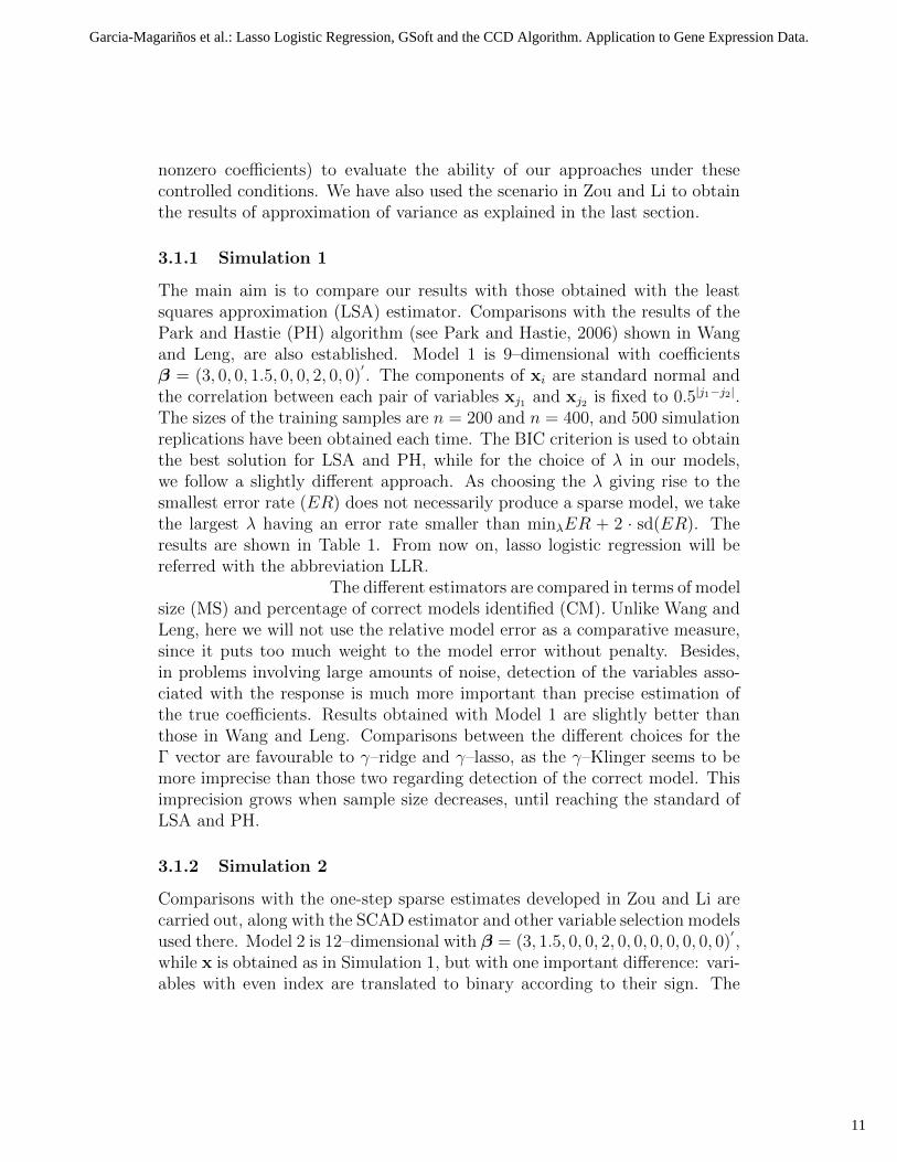
the correlation between each pair of variables xj1 and xj2 is fixed to 0.5|j1−j2|.The sizes of the training samples are n = 200 and n = 400, and 500 simulationreplications have been obtained each time. The BIC criterion is used to obtainthe best solution for LSA and PH, while for the choice of λ in our models,we follow a slightly different approach. As choosing the λ giving rise to thesmallest error rate (ER) does not necessarily produce a sparse model, we takethe largest λ having an error rate smaller than minλER + 2 · sd(ER). Theresults are shown in Table 1. From now on, lasso logistic regression will bereferred with the abbreviation LLR.

The different estimators are compared in terms of modelsize (MS) and percentage of correct models identified (CM). Unlike Wang andLeng, here we will not use the relative model error as a comparative measure,since it puts too much weight to the model error without penalty. Besides,in problems involving large amounts of noise, detection of the variables asso-ciated with the response is much more important than precise estimation ofthe true coefficients. Results obtained with Model 1 are slightly better thanthose in Wang and Leng. Comparisons between the different choices for theΓ vector are favourable to γ–ridge and γ–lasso, as the γ–Klinger seems to bemore imprecise than those two regarding detection of the correct model. Thisimprecision grows when sample size decreases, until reaching the standard ofLSA and PH.

3.1.2 Simulation 2

Comparisons with the one-step sparse estimates developed in Zou and Li arecarried out, along with the SCAD estimator and other variable selection modelsused there. Model 2 is 12–dimensional with β = (3, 1.5, 0, 0, 2, 0, 0, 0, 0, 0, 0, 0)

′,

while x is obtained as in Simulation 1, but with one important difference: vari-ables with even index are translated to binary according to their sign. The

11


Sample Estimation MS CMsize method mean (SE) mean (SE)200 LLR γ–Klinger 3.266 (0.025) 0.762 (0.019)

LLR γ–ridge 2.896 (0.025) 0.812 (0.017)LLR γ–lasso 2.96 (0.028) 0.798 (0.018)

LSA 3.178 (0.026) 0.798 (0.018)PH 3.272 (0.033) 0.716 (0.020)

400 LLR γ–Klinger 3.046 (0.011) 0.956 (0.009)LLR γ–ridge 2.964 (0.021) 0.860 (0.016)LLR γ–lasso 2.982 (0.022) 0.902 (0.013)

LSA 3.130 (0.018) 0.888 (0.014)PH 3.092 (0.023) 0.846 (0.016)

Table 1: True model detection results. Comparison between Model 1 and those inWang and Leng is established in the same terms as there.

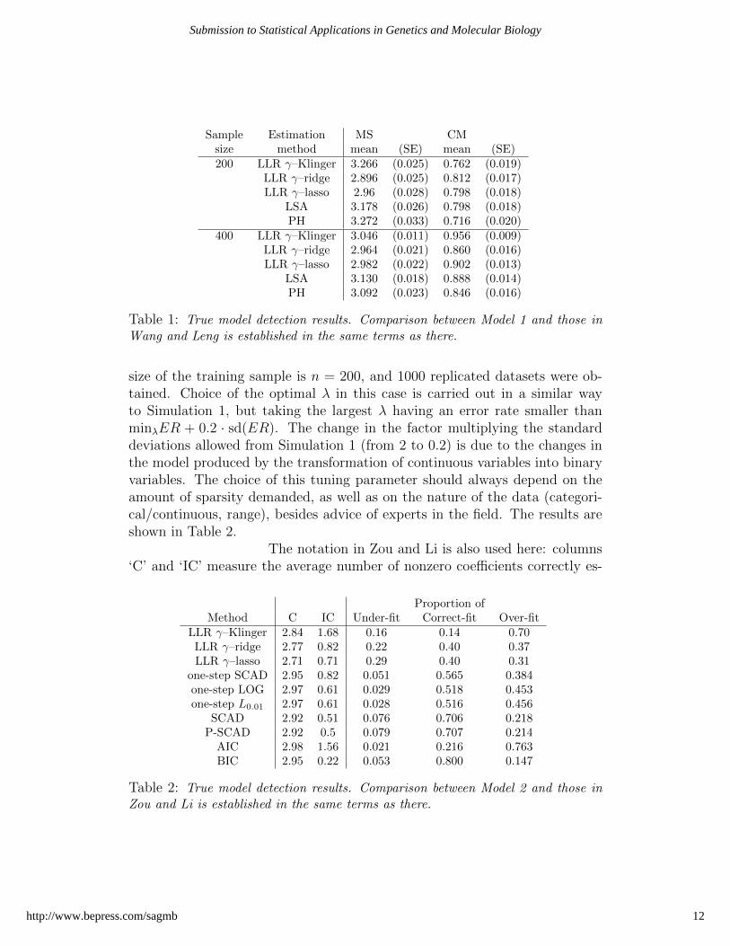
size of the training sample is n = 200, and 1000 replicated datasets were ob-tained. Choice of the optimal λ in this case is carried out in a similar wayto Simulation 1, but taking the largest λ having an error rate smaller thanminλER + 0.2 · sd(ER). The change in the factor multiplying the standarddeviations allowed from Simulation 1 (from 2 to 0.2) is due to the changes inthe model produced by the transformation of continuous variables into binaryvariables. The choice of this tuning parameter should always depend on theamount of sparsity demanded, as well as on the nature of the data (categori-cal/continuous, range), besides advice of experts in the field. The results areshown in Table 2.

The notation in Zou and Li is also used here: columns‘C’ and ‘IC’ measure the average number of nonzero coefficients correctly es-

Proportion ofMethod C IC Under-fit Correct-fit Over-fit

LLR γ–Klinger 2.84 1.68 0.16 0.14 0.70LLR γ–ridge 2.77 0.82 0.22 0.40 0.37LLR γ–lasso 2.71 0.71 0.29 0.40 0.31

one-step SCAD 2.95 0.82 0.051 0.565 0.384one-step LOG 2.97 0.61 0.029 0.518 0.453one-step L0.01 2.97 0.61 0.028 0.516 0.456

SCAD 2.92 0.51 0.076 0.706 0.218P-SCAD 2.92 0.5 0.079 0.707 0.214

AIC 2.98 1.56 0.021 0.216 0.763BIC 2.95 0.22 0.053 0.800 0.147

Table 2: True model detection results. Comparison between Model 2 and those inZou and Li is established in the same terms as there.

12



ρ = 0.25 ρ = 0.75Method C I C I

LLR γ–Klinger 5.96 0.034 5.562 0.326LLR γ–ridge 5.9 0.166 5.912 0.778LLR γ–lasso 5.9 0.176 5.916 0.76

New 5.922 0 5.534 0.222LQA 5.728 0 4.97 0.090BIC 5.86 0 5.796 0.304AIC 4.93 0 4.86 0.092

Table 3: True model detection results. Comparison between Model 2 and those inHunter and Li is established in the same terms as there.

timated to be nonzero and the average number of zero coefficients incorrectlyestimated to be nonzero, respectively. “Under–fit” and “Over–fit” show theproportion of models excluding any nonzero coefficients and including any zerocoefficients throughout the 1000 replications, respectively. “Correct–fit” showsthe proportion of correct models obtained.

Our methods show a worse behaviour than those in Zouand Li. After some tests (results not shown here) we realized that the reasonwas that they suffer a lot from the presence of binary variables. This is not amajor concern, since our aim was to apply these methods to gene expressiondata, where all the variables are continuous. Therefore, in order to test themin a continuous environment, conditions in Hunter and Li were replicated.These conditions are the same as in Simulation 1 but the correlation betweenvariables is now fixed to ρ = 0.25 and ρ = 0.75. The sample size was also fixedto n = 200. The results are shown in Table 3.

The optimal λ is chosen as in Simulation 1. The columns“C” and “I” measure the average number of coefficients correctly and incor-rectly set to zero, respectively. Comparisons are made with a new algorithmproposed in Hunter and Li, a local quadratic approximation (LQA) algorithmdeveloped in Fan and Li and the best subset variable selection using BIC andAIC scores. Competitive results are obtained with respect to the procedure inHunter and Li. The best variable selection is obtained using BIC. The resultsobtained with the γ–Klinger are similar to the ones with γ–ridge and γ–lasso.

3.1.3 Simulation 3

We also performed a new simulation to emulate the conditions of a gene ex-pression study. As a consequence, the same conditions as in Simulation 1were recreated here, but now for a 1000-dimensional model, where just 10 co-efficients (chosen at random in each simulation replication) take the nonzero

13


Sample Method MS PC PN Ratiosize mean (SE) mean (SE) mean (SE)100 LLR γ–Klinger 8.95 (3.02) 0.373 (0.093) 0.005 (0.003) 0.72

LLR γ–ridge 7.93 (6.28) 0.331 (0.120) 0.005 (0.005) 0.68LLR γ–lasso 5.72 (3.94) 0.315 (0.096) 0.003 (0.003) 1.22

200 LLR γ–Klinger 17.76 (3.35) 0.674 (0.101) 0.011 (0.003) 0.61LLR γ–ridge 15.15 (9.62) 0.613 (0.118) 0.009 (0.009) 0.68LLR γ–lasso 12.02 (6.67) 0.636 (0.108) 0.006 (0.006) 1.13

400 LLR γ–Klinger 25.53 (4.22) 0.883 (0.074) 0.016 (0.004) 0.52LLR γ–ridge 20.59 (11.78) 0.833 (0.091) 0.012 (0.011) 0.68LLR γ–lasso 13.77 (6.48) 0.852 (0.085) 0.005 0.006 1.62

Table 4: True model detection results. Comparison is established in terms of detec-tion of noise and true nonzero coefficients for a high dimensional simulation study.

values (3, 1.5, 7, 4, 2.2, 1, 10, 2, 5, 3)′. Apart from the training sample sizes used

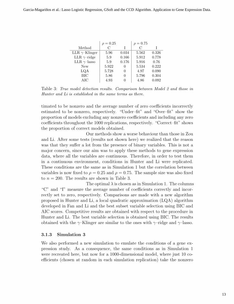
in Simulation 1 (n = 200 and n = 400), a new one (n = 100) was added.Since the presence of so much noise covariates and the correlation structuregives rise to high variability for the error rate measures, we took the largestλ having an error rate smaller than minλER + 0.2 · sd(ER). The results areshown in Table 4.

Comparisons were established in terms of model size(MS), understood as the number of nonzero coefficients estimated, proportionof nonzero coefficients correctly estimated as nonzero (PC), and proportionof noise in the models (PN), understood as the proportion of zero coefficientsestimated nonzero. The right column refers to the ratio of correct nonzerocoefficients to incorrect nonzero coefficients for the model selected.

The results show a clear trend towards increasing modelsizes when sample size grows. It is essential to recall the fact that model sizesin Table 4 strongly depend on the penalization (λ), and therefore on the factormultiplying the standard deviation selected above (0.2). The larger this fac-tor, the smaller the model size. Considering similar model sizes, γ–ridge and,above all, γ–lasso, show higher proportions of nonzero coefficients correctlyidentified (PC). Many of the incorrect nonzero coefficients in the estimatedmodels correspond with covariates correlated with the true nonzero ones (re-sults not shown here). Figure 1 shows the changes in model size (MS), numberof true nonzero (NC) and true zero (NN) detected coefficients, and Ratio, allof them averaged, when the λ penalization (or the number of standard devia-tions) varies, for the γ–lasso approach and different sample sizes. The PC andPN values which appear in Table 4 are, respectively, the NC and NN valuesexpressed as proportions.

14



Figure 1: Changes in model detection for the γ–lasso approach and different samplesizes: n = 100 (left) and n = 400 (right), when the penalization term λ varies. Asindicated in the legends, the black line denotes the model size (MS), as the averagenumber of detected nonzero coefficients. This MS is the result of adding the numberof true nonzero (NC, red line) and the number of true zero (NN, green line) detectedas nonzero (both averaged). The Ratio (blue line) is the result of dividing NC byNN.

3.1.4 Approximation of variance

Covariance matrix estimation for the estimated coefficients has been obtainedaccording to the previously explained approach. Model 2 has been used, with-out the translation to binary (for simplicity). In Figure 2, the behaviour ofvariance estimation for β1 = 3, β2 = 1.5 and β3 = 0, respectively, is shownin comparison with the true variance, as a function of λ. The estimation,obtained as the median along 1000 replications, fits almost perfectly to thevariance except for small deviations when λ is close to zero (maximum likeli-hood estimator), as the true variance increases enormously.

3.2 Real data.

The leukemia dataset (Golub et al., 1999) has been used on countless occasionsthrough the gene expression literature. It comprises gene expression data for72 bone marrow and peripheral blood samples (47 cases of acute lymphoblasticleukemia (ALL) and 25 cases of acute myeloid leukemia (AML)) in 7129 genes.Initially (Golub et al.) the total sample was divided into a training sample

15


(38 bone marrow samples) and a test sample (34 bone marrow and peripheralblood samples).

The colon dataset was analyzed initially by Alon et al.(1999). As leukemia, it is another commonly used dataset in genomic stud-ies. A number of 62 observations (40 tumors and 22 controls) were measuredin 2000 human genes. Absolute measurements from Affymetrix high–densityoligonucleotide arrays were taken for each sample in each gene in both datasets.Here, we have worked with data in two different ways. On one side, we havecarried out preprocessing steps (P) following Subsection 3.1.2 of Dudoit etal. (2002), (i) thresholding of the measurements, (ii) filtering of genes, (iii)base 10 logarithmic transformation. On the other hand, we have also triedour models over the raw data (RD). With preprocessing, leukemia and colondatasets reduce their dimensionality to 3571 and 1225 genes, respectively.

As a result of combining these two ways to deal withdata with the three different choices for γ, we have six different procedures.Table 5 shows the results for the leukemia dataset. To obtain accurate andprecise measures for the error and its standard deviation, we randomly split50 times the set of 72 samples into a training set of 38 samples and a test setof 34 samples. We also record the number of genes with non-zero coefficientfor the optimal lambda, in terms of cross–validation (CV) error.

Figure 2: Variance estimation (in red) for the estimated values of β1, β2 and β3

in Simulation 2, according to the estimator (17) with F taken as in (20). Truevariance (in black) was approximated by means of recursive simulation–estimation.The variance is displayed as a function of the penalty parameter λ.

16



Leukemia Test error SD GenesRD-γ Klinger 0.062 (0.044) 67 (of 7129)

RD-γ Zou 0.064 (0.039) 11 (of 7129)RD-γ Lasso 0.102 (0.055) 6 (of 7129)P-γ Klinger 0.079 (0.032) 16 (of 3571)

P-γ Zou 0.067 (0.030) 5 (of 3571)P-γ Lasso 0.064 (0.028) 5 (of 3571)

Table 5: Test error and sparsity results for the leukemia dataset.

Colon Test error SD GenesRD-γ Klinger 0.195 (0.130) 10 (of 2000)

RD-γ Zou 0.147 (0.116) 17 (of 2000)RD-γ Lasso 0.200 (0.128) 9 (of 2000)P-γ Klinger 0.152 (0.096) 11 (of 1225)

P-γ Zou 0.182 (0.111) 15 (of 1225)P-γ Lasso 0.215 (0.133) 10 (of 1225)

Table 6: Test error and sparsity results for the colon dataset.

Table 6 shows the results for the colon dataset. The62–sample has been randomly splitted 50 times into a training subsample of50 observations and a test subsample of 12 observations. Different ways ofsplitting for the two real datasets are explained from their different nature.An unbalanced train-test data split is needed in the colon dataset to detectthe existing associations (see Krishnapuram et al., 2005).

Leukemia and colon datasets have been often used inthe literature to test the performance of different methods. Nevertheless, it isdifficult to find a fair comparison between methods, since each author uses adifferent way to obtain an error measure. Some of them only focus on a leave–one–out cross–validation rate (too optimistic); others center on the same datasubdivision carried out by Golub et al. Finally, the fairest way to know thereal performance of each method is to randomly split the total sample N timesinto two disjoint samples, training and test. Table 7 compares our best testerror results with those from other methods, using similar training-testing datadivisions.

Comparisons with the following methods have been es-tablished. In Boulesteix et al. (2003), a CART-based method is developed todiscover the emerging patterns within the set of variables. BagBoosting (Det-tling, 2004) is a combination of bagging and boosting, two ensemble learningalgorithms, applied to stumps, decision trees with only one split and two ter-minal nodes. Different algorithms are presented in Dettling and Buhlmann(2004). Pelora is a penalized logistic regression method. Forsela is simi-

17


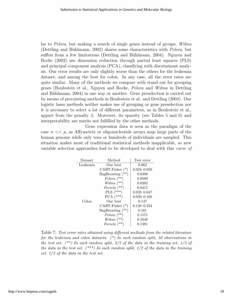
lar to Pelora, but making a search of single genes instead of groups, Wilma(Dettling and Buhlmann, 2002) shares some characteristics with Pelora, butsuffers from a few limitations (Dettling and Buhlmann, 2004). Nguyen andRocke (2002) use dimension reduction through partial least squares (PLS)and principal component analysis (PCA), classifying with discriminant analy-sis. Our error results are only slightly worse than the others for the leukemiadataset, and among the best for colon. In any case, all the error rates arequite similar. Many of the methods we compare with stand out for groupinggenes (Boulesteix et al., Nguyen and Rocke, Pelora and Wilma in Dettlingand Buhlmann, 2004) in one way or another. Gene preselection is carried outby means of preexisting methods in Boulesteix et al. and Dettling (2004). Ourlogistic lasso methods neither makes use of grouping or gene preselection norit is necessary to select a lot of different parameters, as in Boulesteix et al.,appart from the penalty λ. Moreover, its sparsity (see Tables 5 and 6) andinterpretability are merits not fulfilled by the other methods.

Gene expression data is seen as the paradigm of thecase n << p, as Affymetrix or oligonucleotide arrays map large parts of thehuman genome while only tens or hundreds of individuals are sampled. Thissituation makes most of traditional statistical methods inapplicable, so newvariable selection approaches had to be developed to deal with this curse of

Dataset Method Test errorLeukemia Our best 0.062

CART-Fisher (*) 0.024–0.050BagBoosting (**) 0.0408

Pelora (**) 0.0569Wilma (**) 0.0262Forsela (**) 0.0415PLS (***) 0.033–0.047PCA (***) 0.039–0.108

Colon Our best 0.147CART-Fisher (*) 0.128–0.234BagBoosting (**) 0.161

Pelora (**) 0.1571Wilma (**) 0.1648Forsela (**) 0.1381

Table 7: Test error rates obtained using different methods from the related literaturefor the leukemia and colon datasets. (*) In each random split, 10 observations inthe test set. (**) In each random split, 2/3 of the data in the training set, 1/3 ofthe data in the test set. (***) In each random split, 1/2 of the data in the trainingset, 1/2 of the data in the test set.

18



dimensionality problem. Lasso selects a group of p′ ≤ n genes with high

importance in the classification of samples, and assigns a zero coefficient tothe remaining genes. The use of the CCD algorithm to solve the optimizationproblem is highly desirable, as it provides with the global solution of GSoft inthe fastest and most efficient way.

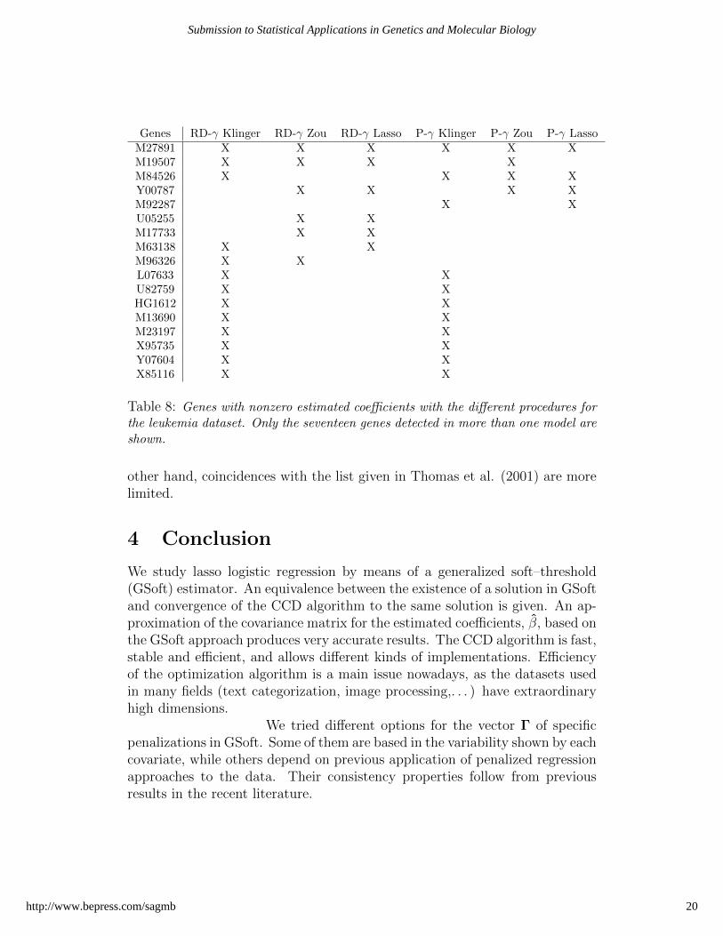
From a more biological view, we have also studied whichgenes are more related with the ALL/AML status in leukemia. Observationsof the genes with nonzero coefficients for each model have been carried out. Asexpected, some recurrences have been found with the six different procedures.Table 8 shows those genes showing up more frequently.

The fact that some genes are discovered with some pro-cedures and not with others can be explained from the correlations betweenthem. These correlations arise as a result of co–inheritance of nearby genesthroughout generations. For instance, gene M19507 takes a nonzero coefficientwith all but two of the procedures, and gene M92287 takes nonzero coefficientsonly with these two procedures. If we take a careful look to the correlationbetween them, we detect it as unusually high. A correlation study between allthe genes with nonzero coefficient in any of the models has been carried out.With the aim of knowing the real meaning of each correlation value, a sim-ple permutation testing was applied: a significance value for each correlationwas obtained as the proportion of values, in a set of 10000 random correla-tions taken between pairs of genes from the entire dataset, which are higherthan the correlation under study. In this way, significance of the correlationM19507–M92287 is 0.0558; the one between M84526–Y00787 is 0.048, whichexplains why they are partly complementary. Significances of correlations be-tween gene Y00787 and the last eight genes in Table 8 are also very low, asthey are detected specifically in those two models where Y00787 is not. In asimilar way, pairwise correlations in this 8–gene group are often high. Com-plementarity in the detection by the different models emphasizes one of themain problems of lasso selection, also marked in Zou and Hastie: when thereis a group of significant variables with high pairwise correlation lasso selectsonly one, and does not care which one.

A bunch of articles can be found in the gene expres-sion literature looking for genes associated with the ALL/AML status. It isexpected that there exists some kind of intersection between the sets of genesgiven by the different studies. The first five genes in the relation of Table 8(M27891, M19507, M84526, Y00787 and M92287) are also discovered in Leeet al. (2003), being M27891 the one showing the strongest association withdisease, as happens here. Three of the four genes pointed out in Guyon etal. (2002) (U82759, HG1612 and X95735) are also discovered here. On the

19


Genes RD-γ Klinger RD-γ Zou RD-γ Lasso P-γ Klinger P-γ Zou P-γ LassoM27891 X X X X X XM19507 X X X XM84526 X X X XY00787 X X X XM92287 X XU05255 X XM17733 X XM63138 X XM96326 X XL07633 X XU82759 X XHG1612 X XM13690 X XM23197 X XX95735 X XY07604 X XX85116 X X

Table 8: Genes with nonzero estimated coefficients with the different procedures forthe leukemia dataset. Only the seventeen genes detected in more than one model areshown.

other hand, coincidences with the list given in Thomas et al. (2001) are morelimited.

4 Conclusion

We study lasso logistic regression by means of a generalized soft–threshold(GSoft) estimator. An equivalence between the existence of a solution in GSoftand convergence of the CCD algorithm to the same solution is given. An ap-proximation of the covariance matrix for the estimated coefficients, β, based onthe GSoft approach produces very accurate results. The CCD algorithm is fast,stable and efficient, and allows different kinds of implementations. Efficiencyof the optimization algorithm is a main issue nowadays, as the datasets usedin many fields (text categorization, image processing,. . . ) have extraordinaryhigh dimensions.

We tried different options for the vector Γ of specificpenalizations in GSoft. Some of them are based in the variability shown by eachcovariate, while others depend on previous application of penalized regressionapproaches to the data. Their consistency properties follow from previousresults in the recent literature.

20



Finally, we applied these methods to simulated dataand gene expression data. The same simulations carried out in other studieswere used here, in order to provide honest and fair comparisons. A highdimensional simulation study was also performed, in order to emulate thecharacteristics of gene expression studies. The best model is selected from theerror rate results, correcting using the standard error. The factor multiplyingthe standard error should be guided by the authors’ prior knowledge about theproblem. Common gene expression datasets, like leukemia or colon, allow toknow the ability of these methods to detect genes related with the disease ortrait under study. The penalized regression approaches performed in this workgive rise to sparse models, where only a very small percentage of covariates(genes) have a positive weight in classification/prediction.

Appendix. Proof of theorem 2

The log–likelihood functions in logistic regression and in lasso logistic regres-sion with specific penalizations are given in (5) and (6), respectively. The firstpartial derivatives or score functions are:

sj(β) =n∑i=1

−yixij1 + exp(yix

′iβ)

(25)

The definition of the ∆vj for the lasso case in Genkinet al., applied on a penalized regression problem with specific penalizations foreach variable, is given in (10). For ease of notation, we will use here S insteadof sign(βj). We will base the entire proof in the steps and the notations usedin Figures 4 and 5 in Genkin et al. Many of the terms used there will berepeated here. To clarify the notation, we will use βj for the true value of the

coefficients and β(I)j for the value of the jth coefficient in the Ith iteration of

the CCD algorithm.We begin by proving the equivalence for the case βj = 0,

and then we will move to the more general case of βj > 0 (similar proof forβj < 0).

Case βj = 0

(1)⇒ (2)We assume that the CCD algorithm, as explained in

Genkin et al., converges. Therefore, from a certain iteration, I, we have β(I)j =

21


0 and ∆v(I)j = 0. The CCD algorithm tries then to improve the objective

function by searching in the positive and the negative direction, so:

{S = 1 and ∆v

(I+1)j ≤ 0 ⇔ sj(β)− λγj ≤ 0

S = −1 and ∆v(I+1)j ≥ 0 ⇔ sj(β) + λγj ≥ 0

}⇔ (26)

{sj(β) ≤ λγj−sj(β) ≤ λγj

}⇔ (27)

⇔ |sj(β)| ≤ λγj (28)

(2)⇒ (1)We assume now that the necessary and sufficient con-

ditions for convergence in the GSoft theorem are fulfilled. This implies

|sj(β)| ≤ λγj (29)

We need to bear in mind also that the initial value forβj in the CCD algorithm is β

(0)j = 0. In this situation and from the definitions

of the CCD algorithm for the lasso case, we have that

• if we try S = 1 (positive direction) then ∆v(0)j ≤ 0 and positive direction

failed.

• if we try S = −1 (negative direction) then ∆v(0)j ≥ 0 and negative

direction failed.

Therefore, following the steps of the CCD algorithm forthe lasso case, this means we take ∆v

(0)j = 0, as both directions failed, and

then

∆βj = min(max(0,−∆j),∆j

)= min

(0,∆j

)= 0 (30)

and the CCD algorithm converges.

Case βj > 0 (the proof is similar for βj < 0)

(1)⇒ (2)Let us suppose that sj(β) 6= λγj and we will show that

this gives rise to a contradiction. As the true βj is positive and the CCDalgorithm converges, from any iteration, I, we will have βJj > 0 for all iteration

22



J > I, so S = 1 and ∆vJj 6= 0, following the definition in (10). Thus, for anypositive constant k,

∆β(J)j = min

(max(∆v

(J)j ,−∆

(J)j ),∆

(J)j

)6= 0 ⇒ (31)

⇒ ∆(J+1)j = max

(2|∆β(J)

j |,∆

(J)j

2

)> k > 0 (32)

and this happens for every iteration J > I, which enters in contradiction withthe convergence of the CCD algorithm to βj.(2)⇒ (1)

We assume now that necessary and sufficient conditionsfor convergence in the GSoft theorem are fulfilled. Let us suppose that theCCD algorithm converges to a different “solution” β 6= β with βj 6= βj.

In such a case, as the conditions in (a) in the GSoft the-

orem determine a unique solution, it has to be sj(β) 6= λγj. Then ∆v(J)j 6= 0,

for all J > I with I ∈ N and therefore ∆βj does not converge to 0, whichmeans the CCD algorithm does not converge either, which is a contradiction.

We have not mentioned or used anywhere in the proofthe condition about the positive definite nature of the matrix X

′

λH(η)Xλ. Sowe have to prove that this condition is also fulfilled when the CCD algorithmconverges. We will prove this by reductio ad absurdum.

Let us assume that X′

λH(η)Xλ is not definite positive.As Xλ is a complete matrix, this implies that H(η) is not definite positive,and therefore

−H(η) (Hessian) is not definite negative∂L1(β)∂βj

= 0 for all j ∈ {1, . . . , p}

}(33)

and therefore the estimated linear predictor, η, cannot be a maximum of theobjective function in Klinger, which means β is not a minimum of the ob-jective function in Genkin et al. and the CCD algorithm does not converge(contradiction).

References

Alon U., Barkai N., Notterman D., Gish K., Ybarra S., Mack D. and LevineA.J. Broad patterns of gene expression revealed by clustering analysis oftumor and normal colon tissues probed by oligonucleotide arrays. Proceed-ings of the National Academy of Sciences USA, 96(12), (1999), 6745–6750.

23


Antoniadis A. and Fan J. Regularization of wavelet approximations. Journalof the American Statistical Association, 96(455), (2001), 939–967.

Antoniadis A., Gijbels I. and Nikolova M. Penalized likelihood regression forgeneralized linear models with nonquadratic penalties. Annals of the Insti-tute of Statistical Mathematics (in press), (2009).

Bakin S. Adaptive regression and model selection in data mining problems.PhD Thesis, Australian National University, Canberra, (1999).

Boulesteix A.L., Tutz G. and Strimmer K. A CART–based approach to discoveremerging patterns in microarray data. Bioinformatics, 19(18), (2003),2465–2472.

De Leeuw J. Block-relaxation methods in statistics. In Bock H.H., LenskiW. and Richter M.M., editors, Information Systems and Data Analysis,Springer-Verlag, Berlin, (1994).

De Mol C., De Vito E. and Rosasco L. Elastic–net regularization in learningtheory. Journal of Complexity, 25(2), (2009), 201–230.

Dettling M. BagBoosting for tumor classification with gene expression data.Bioinformatics, 20(18), (2004), 3583–3593.

Dettling M. and Buhlmann P. Finding predictive gene groups from microarraydata. Journal of Multivariate Analysis, 90, (2004), 106–131.

Dettling M. and Buhlmann P. Supervised clustering of genes. Genome Biology,3(12), (2002), 0069.1–0069.15.

Dudoit S., Fridlyand J. and Speed T.P. Comparison of discrimination methodsfor the classification of tumors using gene expression data. Journal of theAmerican Statistical Association, 97(457), (2002), 77–87.

Efron B., Hastie T., Johnstone I. and Tibshirani R. Least angle regression.Annals of Statistics, 32(2) (2004), 407–499.

Eggermont P.P. and LaRiccia V.N. Maximum penalized likelihood estimation.Vol. 2 Regression, Springer Series in Statistics, New York, (2009).

Fan J. and Li R. Variable selection via nonconcave penalized likelihood andits oracle properties. Journal of the American Statistical Association,96(456), (2001), 1348–1360.

24



Frank I.E. and Friedman J.H. A statistical view of some chemometrics tools.Technometrics, 35(2), (1993), 109–135.

Friedman J., Hastie T. and Tibshirani R. Regularization paths for generalizedlinear models via coordinate descent. Technical Report, Department ofStatistics, Stanford University, (2008).

Genkin A., Lewis D.D. and Madigan D. Sparse logistic regression for textcategorization. DIMACS Working Group on Monitoring Message Streams,Project Report, (2005).

Goldstein T. and Osher S. The Split Bregman method for L1 regularized prob-lems. UCLA CAAM Report 08–29, (2008).

Golub T.R., Slonim D.K., Tamayo P., Huard C., Gaasenbeck M., Mesirov P.,Coller H., Loh M.L., Downing J.R., Caligiuri M.A. et al. Molecular classi-fication of cancer: class discovery and class prediction by gene expressionmonitoring. Science, 286(5439), (1999), 531–537.

Guyon I. and Elisseeff A. An introduction to variable and feature selection.Journal of Machine Learning Research, 3(Mar), (2003), 1157–1182.

Guyon I., Weston J., Barnhill S. and Vapnik V. Gene selection for cancerclassification using support vector machines. Machine Learning, 46(1–3),(2002), 389–422.

Hall M. Correlation–based feature selection for machine learning. PhD The-sis, Department of Computer Science, Waikato University, New Zealand,(1999).

Hoerl A.E. and Kennard R. Ridge regression: biased estimation for nonorthog-onal problems. Technometrics, 12(1), (1970), 55–67.

Huang J., Horowitz J.L. and Ma S. Asymptotic properties of bridge estimatorsin sparse high–dimensional regression models. Technical Report, Depart-ment of Statistics and Actuarial Science, The University of Iowa, (2006).

Huang J., Ma S. and Zhang C.H. Adaptive lasso for sparse high–dimensionalregression models. Statistica Sinica, 18(4), (2008), 1603–1618.

Huang J., Ma S. and Zhang C.H. The iterated lasso for high–dimensional logis-tic regression. Technical report No. 392, The University of Iowa, (2008).

25


Huber P.J. The behavior of maximum likelihood estimates under nonstandardconditions. Proceedings of the Fifth Berkeley Simposium on MathematicalStatistics and Probability, (1967).

Hunter D.R. and Li R. Variable selection using MM algorithms. Annals ofStatistics, 33(4), (2005), 1617–1642.

Kim Y., Choi H. and Oh H.S. Smoothly clipped absolute deviation on highdimensions. Journal of the American Statistical Association, 103(484),(2008), 1665–1673.

Klinger A. Inference in high dimensional generalized linear models based onsoft thresholding. Journal of the Royal Statistical Society Series B, 63(2),(2002), 377–392.

Knight K. and Fu W.J. Asymptotics for lasso–type estimators. Annals of Statis-tics, 28(5), (2000), 1356–1378.

Krishnapuram B., Carin L., Figueiredo M.A.T. and Hartemink A.J. Sparsemultinomial logistic regression: fast algorithms and generalization bounds.IEEE Transactions on Pattern Analysis and Machine Intelligence, 27(6),(2005), 957–968.

Lee S.I., Lee H., Abbeel P. and Ng A.Y. Efficient L1 regularized logistic re-gression. Proceedings of the Twenty–first International Conference on Ma-chine Learning (AAAI-06), (2006).

Lee K.E., Sha N., Dougherty E.R., Vannucci M. and Mallick B.K. Gene se-lection: a bayesian variable selection approach. Bioinformatics, 19(1),(2003), 90–97.

Liu Z., Jiang F., Tian G., Wang S., Sato F., Meltzer S.J. and Tan M. Sparselogistic regression with Lp penalty for biomarker identification. StatisticalApplications in Genetics and Molecular Biology, 6(1), (2007), article 6.

Lv J. and Fan Y. A unified approach to model selection and sparse recoveryusing regularized least squares. Annals of Statistics, 37(6A), (2009), 3498–3528.

Meier L., van de Geer S. and Buhlmann P. The group lasso for logistic re-gression. Journal of the Royal Statistical Society Series B, 70(1), (2008),53–71.

26



Meinshausen N. and Buhlmann P. High dimensional graphs and variable se-lection with the lasso. Annals of Statistics, 34(3), (2006), 1436–1462.

Nguyen D.V. and Rocke D.M. Tumor classification by partial least squaresusing microarray gene expression data. Bioinformatics, 18(1), (2002), 39–50.

Park M.Y. and Hastie T. An L1 regularization–path algorithm for generalizedlinear models. Manuscript, Department of Statistics, Stanford University,(2006).

Roth V. The generalized lasso. IEEE Transactions on Neural Networks, 15,(2004), 16–28.

Schmidt M., Fung G. and Rosales R. Fast optimization methods for L1 regu-larization: a comparative study and two new approaches. European Con-ference on Machine Learning (ECML), (2007).

Shevade S. and Keerthi S. A simple and efficient algorithm for gene selec-tion using sparse logistic regression. Bioinformatics, 19(17), (2003), 2246–2253.

Tarigan B. and van de Geer S. Classifiers of support vector machine type withL1 complexity regularization. Bernoulli, 12(6), (2006), 1045–1076.

Thomas J.G., Olson J.M. and Tapscott S.J. An efficient and robust statisticalmodeling approach to discover diferentially expressed genes using genomicexpression profiles. Genome Research, 11, (2001), 1227–1236.

Tibshirani R. Regression shrinkage and selection via the lasso. Journal of theRoyal Statistical Society Series B, 58(1), (1996), 267–288.

Tseng P. Convergence of block coordinate descent method for nondifferentiablemaximization. Journal of Optimization Theory and Applications, 109,(2001), 473–492.

Tseng P. and Yun S. A coordinate descent gradient method for nonsmoothseparable minimization. Mathematical Programming, 117, (2009), 387–423.

Wang H. and Leng C. Unified lasso estimation via least squares approximation.Journal of the American Statistical Association, 102(479), (2007), 1039–1048.

27


Weston J., Elisseeff A., Scholkopf B. and Tipping M. Use of the zero–norm withlinear models and kernel methods. Journal of Machine Learning Research,3(Mar), (2003), 1439–1461.

Wright S.J., Nowak R.D. and Figueiredo M.A.T. Sparse reconstruction by sep-arable approximation. Proceedings of the IEEE International Conferenceon Acoustics, Speech and Signal Processing (ICASSP), (2008).

Wu T.T. and Lange K. Coordinate descent algorithms for lasso penalized re-gression. Annals of Applied Statistics, 2(1), (2008), 224–244.

Yuan M. and Lin Y. Model selection and estimation in regression with groupedvariables. Journal of the Royal Statistical Society Series B, 68(1), (2006),49–67.

Zhang C.H. and Huang J. The sparsity and bias of the lasso selection in high–dimensional linear regression. Annals of Statistics, 36(4), (2008), 1567–1594.

Zhang T. Some sharp performance bounds for least squares regression with L1regularization. Annals of Statistics, 37(5A), (2009), 2109–2144.

Zhang T. and Oles F. Text categorization based on regularized linear classifiers.Information Retrieval, 4(1), (2001), 5–31.

Zou H. The adaptive lasso and its oracle properties. Journal of the AmericanStatistical Association, 101(476), (2006), 1418–1429.

Zou H. and Hastie T. Regularization and variable selection via the elastic net.Journal of the Royal Statistical Society Series B, 67(2), (2005), 301–320.

Zou H. and Li R. One–step sparse estimates in nonconcave penalized likelihoodmodels. Annals of Statistics, 36(4), (2008), 1509–1533.

28



Documents

An Article Submitted to Statistical Applications in Genetics and ...dm.udc.es/modes/sites/default/files/GarciaMagarinos_Antoniadis_Cao... · that, as opposed to ridge regression (Hoerl