An Approximate Wind Turbine Control System Model for Wind Farm Power Control

This article has been accepted for inclusion in a future issue of this journal. Content is final as presented, with the exception of pagination.

IEEE TRANSACTIONS ON SUSTAINABLE ENERGY 1

An Approximate Wind Turbine Control SystemModel for Wind Farm Power Control

Yi Guo, Student Member, IEEE, S. Hossein Hosseini, Student Member, IEEE, Choon Yik Tang, Member, IEEE,John N. Jiang, Senior Member, IEEE, and Rama G. Ramakumar, Life Fellow, IEEE

Abstract—Wind farm power control is key to reliable large-scalewind integration. The design of a sophisticated wind farm con-troller, however, is challenging partly because there is a lack ofmodels that appropriately simplify the complex overall dynamicsof a large number of wind turbine control systems (WTCSs). In thispaper, using system identification approaches, we develop a simpleapproximate model that attempts to mimic the active and reactivepower dynamics of two generic WTCS models under normal op-erating conditions: an analyticalmodel described by nonlinear dif-ferential equations, and an empirical one by input-output measure-ment data. The approximate model contains two parts—one foractive power and one for reactive—each of which is a third-ordersystem that would have been linear if not for a static nonlinearity.For each generic model, we also provide an identification schemethat sequentially determines the approximate model parameters.Finally, we show via simulation that, despite its structural sim-plicity, the approximate model is accurate and versatile, capable ofclosely imitating several different analytical and empirical WTCSmodels from the literature and from real data. The results suggestthat the approximate model may be used to facilitate research onwind farm power control.

Index Terms—Approximate model, wind turbine control system,wind farm, power control.

BASIC NOMENCLATUREGeneral

Time.

Actual active and reactive powers.

Desired active and reactive powers.

Steady-state values of actual powers.

Wind speed.

Operating region.

Analytical Model

State variables.

Internal control signals.

Internal feedback signals.

Manuscript received July 23, 2011; revised August 03, 2012; acceptedSeptember 03, 2012. This work was supported by the National ScienceFoundation under Grant ECCS-0926038 and Grant ECCS-0955265.Y. Guo, S. H. Hosseini, C. Y. Tang, and J. N. Jiang are with the School of

Electrical and Computer Engineering, University of Oklahoma, Norman, OK73019 USA (e-mail: [email protected]; [email protected]; [email protected];[email protected]).R. G. Ramakumar is with the School of Electrical and Computer Engi-

neering, Oklahoma State University, Stillwater, OK 74078 USA (e-mail:[email protected]).Color versions of one or more of the figures in this paper are available online

at http://ieeexplore.ieee.org.Digital Object Identifier 10.1109/TSTE.2012.2217992

Empirical Model

Sampling period.

Number of data points.

Approximate Model

Static nonlinear elements.

Time constants.

Filter outputs.

Damping ratios.

Natural frequencies.

Scalar gains.

I. INTRODUCTION

B EING able to control a wind farm so that its power outputis cooperatively maximized, or smoothly regulated, is

imperative to successful and reliable integration of large-scalewind generation into the power grid. The design of a sophis-ticated wind farm control system (WFCS) for such control,however, is challenging for a variety of reasons. First, a windturbine, by itself, is already a fairly complex system withhighly nonlinear dynamics, strong electromechanical coupling,inherently uncertain parameters, and multiple control variables.Second, when hundreds of such turbines are immersed in a windfield across a geographical region, they produce turbulenceand wake effects that affect downstream turbines, causing theiroverall behavior to be complicated. Third, the large number ofcontrol variables to simultaneously handle, and the rich set ofapproaches to possibly use, further compound the complexity.Thus, it is challenging to design a WFCS, which perhaps is areason why there has been relatively little work to date on thetopic [1]–[7], compared to, say, single-turbine control (e.g.,[8]–[19]).One way to cope with the complexities, adopted in [1]–[7],

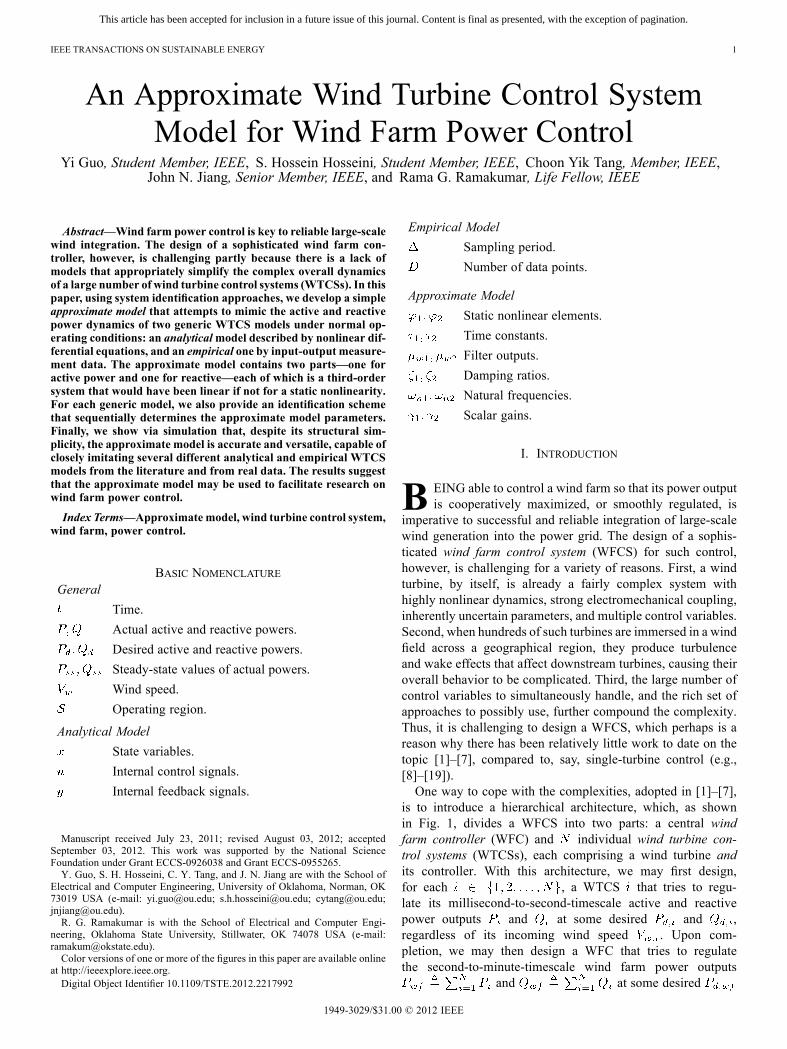
is to introduce a hierarchical architecture, which, as shownin Fig. 1, divides a WFCS into two parts: a central windfarm controller (WFC) and individual wind turbine con-trol systems (WTCSs), each comprising a wind turbine andits controller. With this architecture, we may first design,for each , a WTCS that tries to regu-late its millisecond-to-second-timescale active and reactivepower outputs and at some desired and ,regardless of its incoming wind speed . Upon com-pletion, we may then design a WFC that tries to regulatethe second-to-minute-timescale wind farm power outputs

and at some desired

1949-3029/$31.00 © 2012 IEEE


2 IEEE TRANSACTIONS ON SUSTAINABLE ENERGY

Fig. 1. Hierarchical architecture of a wind farm control system.

and , presumably from a grid operator, by adjustingthe ’s and ’s based on feedback of the ’s and ’sand possibly estimates of the ’s. Hence, the architecturesimplifies the design of a WFCS, allowing us to sequentiallytackle two (seemingly) easier problems on different timescales,as opposed to tackling a harder one. The architecture also offersus the option of designing a new single-turbine controller foreach WTCS , or applying an existing one (e.g., [8]–[14]) thataccepts and as inputs.1 Furthermore, it allows us toview the WFC as a second-to-minute-timescale supervisor thattells every WTCS how much power to generate, and focus onits design without delving too much into millisecond-to-second,turbine-level details.Although the hierarchical architecture makes the problem

more manageable, it does not remove the fact that eachWTCS—being a composition of an already-complex windturbine and a possibly-complicated controller—typically hascomplex dynamics. As a result, the subsequent design andanalysis of a supervisory WFC may prove to be difficult,depending on our goal: if we are content with a simple design(e.g., distribute and evenly among the ’s and

’s, or proportionally based on the ’s) and a basicanalysis (e.g., simulation studies only), then how complex aWTCS is probably does not matter. However, if we aim fora nifty design (e.g., adjust the ’s and ’s so that theWTCSs can exploit their correlation, interaction, and/or di-versity to cooperatively achieve faster transient responses andbetter steady-state smoothness in and ) and a deeperanalysis and understanding (e.g., theoretical characterizationof the resulting transient and steady-state behaviors), then anoverly complex WTCS may render the process very difficult oreven impossible. Therefore, to achieve the latter, it is necessaryto build a suitably simplified WTCS model.To this end, suppose we have developed, or are given,

a WTCS under normal operating conditions—call itWTCS —and wish to design a WFC. Also suppose, atour disposal, is a mathematical model parameterized by avector —call it WTCS —which, like WTCS (or each WTCSin Fig. 1), maps inputs to outputs , i.e.,

. Consider the following con-ditions on the model WTCS :(C1) There exists a such that whenever WTCS and

WTCS are driven by the same inputs ,they produce approximately the same outputs .

1Single-turbine controllers that do not accept and , such as thosethat always attempt maximum power tracking (e.g., [15]–[19]), may not fit wellwith this architecture.

(C2) WTCS may be a nonlinear dynamical system but hasa favorable structure conducive to control systems anal-ysis and design.

(C3) There is a set of WTCSs in the literature such that foreach WTCS in the set, there exists a such that when-ever WTCS and the WTCS are driven by the same in-puts , they produce approximately the sameoutputs .

Note that if (C1) holds, WTCS —with the specific valueof —would be an accurate approximation of WTCS and,thus, may be used in place of WTCS in the WFC design andWFCS analysis. If, in addition, (C2) holds, the design andanalysis would be more likely to succeed due to the favorablestructure of WTCS . If (C3) holds as well, WTCS —withdifferent values of —would be able to also approximate anumber of different WTCSs in the literature (or by differentmanufacturers), making it a versatile model that brings WTCSand those WTCSs under the same umbrella, distinguished onlyby . It follows that the design and analysis outcomes (e.g.,new control techniques, stability criteria, and performanceformulas) are applicable not only to WTCS , but perhaps alsoto those WTCSs, increasing their impact. Hence, having anapproximate model WTCS that satisfies conditions (C1)–(C3)is extremely valuable.This paper is devoted to the development of such a model.We

first assume, in Section II, that two generic models of WTCSare given, namely, an analytical model described by a set ofcontinuous-time nonlinear differential equations, and an em-pirical model described by a set of input-output measurementdata. The latter is motivated by the fact that in practice, what isavailable may just be a set of data, rather than a mathematicalmodel, due to legacy and proprietary reasons. Based on stan-dard system identification approaches [20] and typical WTCScharacteristics, we then develop, in Section III, an approximatemodel WTCS , which attempts to imitate both the analyticaland empirical models. For each of these two models, we alsoprovide a parameter identification scheme that sequentially de-termines the required in (C1), which is a vector of 10 parame-ters (two functions and eight scalars). The approximate model,depicted later in Fig. 3(c), may be regarded as satisfying (C2)because it is made up of two structurally identical parts—onefor active power and the other for reactive—each of which isa third-order system that would have been linear if not for astatic nonlinear component at its inputs (i.e., a modified Ham-merstein model [20], [21]). Next, we validate, in Section IV, theapproximate model via simulation, showing that it has enoughingredients to closely imitate several different analytical andempirical models from the literature [1], [4], [14], [16] and fromreal data taken from an Oklahoma wind farm. The encouragingresults suggest that the approximate model satisfies (C3) and,hence, may be used to facilitate the design and analysis of asecond-to-minute-timescale supervisory WFC that yields a so-phisticated WFCS. Finally, Section V concludes the paper.We stress that this paper is not about wind turbine modeling

(as in, say, [22]–[24]), controller design (as in, say, [8]–[19]),and controller comparison ([4]), nor is it about wind farm mod-eling ([25]–[27]) and controller design ([1]–[7]). Rather, thepaper is on wind turbine control system modeling—not just the


GUO et al.: APPROXIMATE WIND TURBINE CONTROL SYSTEM MODEL FOR WIND FARM POWER CONTROL 3

turbine, but the turbine plus its controller—in the context of thearchitecture in Fig. 1, for which there seems to be no prior work.We note that there has been significant efforts by the WesternElectricity Coordinating Council (WECC), Utility Wind Inte-gration Group (UWIG), and IEEE on developing genericWTCSmodels [28]–[30]. Such models, however, are intended for ac-curately simulating the impact of wind turbine generator dy-namics on power system transient stability without compro-mising vendor proprietary information, rather than for facili-tating research on wind farm power control in the aforemen-tioned context, where model simplicity is at premium. There-fore, those models and our approximate model have notably dif-ferent purposes. Indeed, they have very different structure andlevel of details, which can be seen by comparing, for instance,[28, Figs. 1, 3, and 20–24] with Fig. 3(c) of this paper.

II. MODELS OF WIND TURBINE CONTROL SYSTEMS

In this section, we describe a generic analytical model anda generic empirical model of a WTCS under normal operatingconditions. These two models set the stage for the developmentof an approximate model that mimics the dynamic performanceof the WTCS, when it provides primary generation services tothe grid.

A. Analytical Model

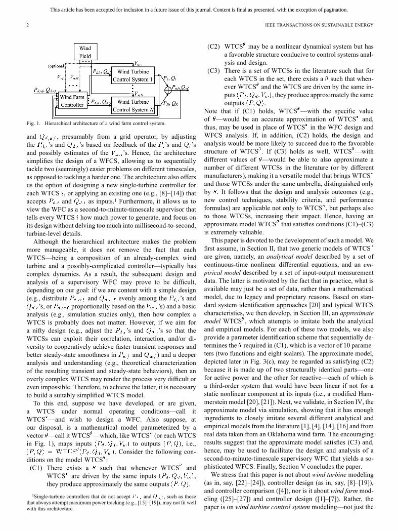
To control a variable-speed wind turbine, a standard approachis to first model its dynamics based on first principles, and thendesign a controller based on known techniques. Regardless ofthe model and design, the resulting wind turbine control system(WTCS) typically can be represented in a block diagram form asin Fig. 2, and described generically by a set of continuous-time,nonlinear differential equations in state-space form as follows:

(1)

(2)

Here, denotes time; is the system statescombining the wind turbine states (e.g., stator and rotor fluxesor currents, rotor angular velocity) and controller states (ifany); is the initial states; and are functions dependingon the particular wind turbine model (e.g., fourth-order [22]or second-order [23] doubly fed induction generator (DFIG)dynamics or second-order permanent magnet synchronous gen-erator (PMSG) dynamics [24], and rigid-shaft or flexible-shaft[23] mechanical dynamics) and the particular controller design(e.g., one of the designs in [1]–[3] and [8]–[14]) includingtheir parameters (e.g., resistances, inductances, rotor momentof inertia, rotor swept area, -surface, air density, frictioncoefficient, controller gains); , , , and are,respectively, the system inputs and outputs representing thedesired and actual active and reactive powers, where positivevalues mean toward the grid; is another system inputrepresenting the wind speed; is the internal control signals(e.g., rotor voltages, blade pitch angle, electromagnetic torque);and is the internal feedback signals (e.g., various voltagesand currents, rotor angular velocity, actual powers).

Fig. 2. Block diagram of a wind turbine control system.

In this paper, we assume that a generic analytical modelof a WTCS, in the form of (1) and (2), is given as the firstof two models considered. In order to represent as manyWTCSs in the literature as possible, we make only two as-sumptions about the analytical model (1) and (2): first, theinputs are always in a bounded operatingregion .Second, the WTCS is reasonably well-designed, i.e.,the functions and are such that for each constant

, there existsteady-state values , depending possibly on

, such that for every ,. Finally, we allow and to be absent,

since many existing WTCSs do not consider the reactive power(e.g., [10]–[12]), and to be absent as well, since some ex-isting WTCSs do not require it to be specified (e.g., [15]–[19]).However, we require and to be present, since theyare essential to WTCSs.

B. Empirical Model

Although it is common to work with a mathematical modelin research on WTCSs, in practice we may not have access tothe inner working of a WTCS, due perhaps to legacy and pro-prietary reasons. Instead, what may be available to us is a set ofinput-output measurement data, so that we have no choice butto treat the WTCS as a “black box.” The set of data can takevarious forms, but more often than not includes the followinginformation:

(3)

where is the sampling period which is usually on theorder of seconds or minutes, and is the number of data pointswhich is usually large.In this paper, we assume that a generic empirical model of

a WTCS, in the form of (3), is given as the second of the twomodels considered. Similar to the analytical model (1) and(2), in the empirical model (3) the columns ,and are optional but the columns andare mandatory. However, unlike the analytical one wherethe inputs can be arbitrarily specified,with this empirical model we have no control over the inputs

, as they are simply given, in thefirstthree columns. This difference will be accounted for shortly.Remark 1: The two models of WTCSs in this section may be

thought of as the WTCS in Section I.



C. Discussion

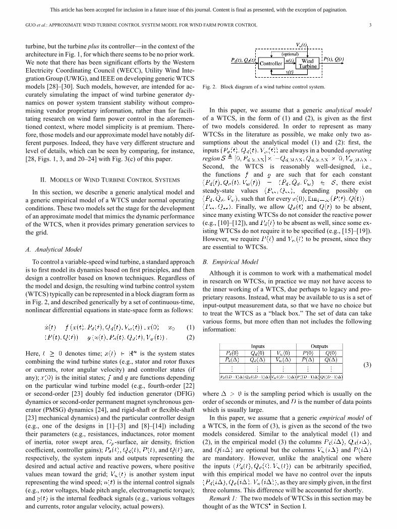
The analytical model (1) and (2) and the empirical model (3)are what our approximate model intends to imitate. As will bedescribed in Section III, our approach is based on postulating astatic nonlinearmodel thatmatches the steady-state input-outputcharacteristics, followed by enriching the model with linear dy-namics so that it also matches the transient input-output behav-iors.A benefit of this input-output approach is that it bypasses theneed to consider the internal dynamics and specific details of theunderlying WTCS, thereby allowing major types of generationtechnologies such as DFIG, PMSG, and IG to be approximatelydescribedusingasimple, consistentmodel.More important, suchamodel enables one to approximately describe a large number ofsame or different types ofWTCSswithin awind farm in a unifiedfashion, so that researchers may focus on other pressing issueswhen designing a comprehensive WFCS and understanding itsattainable performance.

III. PROPOSED APPROXIMATE MODEL

In this section, we develop a simple mathematical modelthat approximates the analytical and empirical WTCS modelsin Section II, and a parameter identification scheme that de-termines the model parameters in each case. The developmentconsists of three steps in both cases, as described below.

A. Approximating the Analytical Model

Step 1: Mimicking the steady-state responses to constantinputsIn general, to create a system that mimics another system, it

is reasonable to demand that the two systems exhibit the samesteady-state responses to constant inputs. With this in mind, wenote that whenever the analytical model (1) and (2) is subject toconstant inputs , its out-puts asymptotically converge to some steady-statevalues , which depend only on and noton the initial states . This dependency suggests that thereexist functions and , such that

and . It also sug-gests a static nonlinear model of the form

(4)

(5)

which is capable of mimicking—at the very least—the steady-state outputs of the analytical model (1) and (2) whenever theinputs are constant, or slow-varying. To visually connect thisStep 1 with subsequent steps of the development, a block dia-gram of the model (4) and (5) is shown in Fig. 3(a).Remark 2: Throughout the paper, the subscripts 1 and 2 are

used to distinguish between similar parameters or variables as-sociated with the active and reactive powers [e.g., is for ac-tive and is for reactive in Fig. 3(a)].The functions and are (infinite-dimensional) parame-

ters of the model (4) and (5), which can be identified by sim-ulating the analytical model (1) and (2) with various constantinputs sufficiently covering the operating region , observingthe steady-state outputs, and employing interpolation. The fol-lowing procedure provides the details:

Fig. 3. Step-by-step development of the proposed approximate model.(a) Block diagram after Step 1 of 3. (b) Block diagram after Step 2 of 3.(c) Block diagram after Step 3 of 3.

Procedure for Step 1

1) Pick a large .2) Pick for .3) Pick a large .4) Loop over .5) Let

.6) Pick any .7) Simulate the analytical model (1) and (2) fromto .

8) Record .9) Let and

.10) End loop.11) Determine and via interpolation on the data

points obtained.

Applying the above procedure to identify the functionsand , we obtain a basic model (4) and (5) that exhibits thesame steady-state behavior as that of (1) and (2).Step 2: Mimicking the transient responses to staircase

inputsThe basic model (4) and (5) in Fig. 3(a) is able to match the

steady-state response of the analytical model (1) and (2). How-ever, it fails to produce any kind of transient one normally wouldexpect with WTCSs because (4) and (5) are merely static func-tions mapping the inputs to the outputs



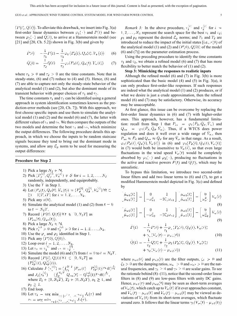
. To alleviate this drawback, we insert into Fig. 3(a)first-order linear dynamics between and and be-tween and , to arrive at a Hammerstein model (see[21] and [20, Ch. 5.2]) shown in Fig. 3(b) and given by

(6)

(7)

where and are the time constants. Note that insteady-state, (6) and (7) reduce to (4) and (5). Hence, (6) and(7) are able to capture not only the steady-state behavior of theanalytical model (1) and (2), but also the dominant mode of itstransient behavior with proper choices of and .The time constants and can be identified using a general

approach in system identification sometimes known as the pre-diction-error methods (see [20, Ch. 7]). With this approach, wefirst choose specific inputs and use them to simulate the analyt-ical model (1) and (2) and the model (6) and (7), the latter withdifferent values of and .We then compare the outputs of thetwo models and determine the best and , which minimizethe output differences. The following procedure details this ap-proach, in which we choose the inputs to be random staircasesignals because they tend to bring out the dominant mode insystems, and allow any norm to be used for measuring theoutput differences:


1) Pick a large .2) Pick forrandomly, independently, and equiprobably.

3) Use the in Step 1.4) Let

for .5) Pick any .6) Simulate the analytical model (1) and (2) fromto .

7) Record as.

8) Pick a large .9) Pick and for .10) Use the and identified in Step 1.11) Pick any .12) Loop over .13) Let and .14) Simulate the model (6) and (7) from to .15) Record as

.16) Calculate

and ,where , and

.17) End loop.18) Let and

.

Remark 3: In the above procedure, and forrepresent the search space for the best and ;

and represent the desired norms; and and areintroduced to reduce the impact of the initial states [i.e., ofthe analytical model (1) and (2) and of the model(6) and (7)] on the parameter estimation process.Using the preceding procedure to identify the time constantsand , we obtain a refined model (6) and (7) that has more

flexibility to better match the behavior of (1) and (2).Step 3: Mimicking the responses to realistic inputsAlthough the refined model (6) and (7) in Fig. 3(b) is more

sophisticated than the basic model (4) and (5) in Fig. 3(a), itcan only produce first-order-like responses. If such responsesare indeed what the analytical model (1) and (2) produces, or ifwhat we desire is just a crude approximation, then the refinedmodel (6) and (7) may be satisfactory. Otherwise, its accuracymay be unacceptable.At first glance, this issue can be overcome by replacing the

first-order linear dynamics in (6) and (7) with higher-orderones. This approach, however, has a fundamental limita-tion: recall from Step 1 that and

. Thus, if a WTCS does powerregulation and does it well over a wide range of , then

and for any in that range. As a result,in (6) and

in (7) would both be insensitive to , so that even largefluctuations in the wind speed would be completelyabsorbed by and , producing no fluctuations inthe active and reactive powers and , which may beunrealistic.To bypass this limitation, we introduce two second-order

linear filters and add two linear terms to (6) and (7), to get amodified Hammerstein model depicted in Fig. 3(c) and definedby

(8)

(9)

(10)

(11)

where and are the filter outputs, andare the damping ratios, and are the nat-

ural frequencies, and and are scalar gains. To seethe rationale behind (8)–(11), notice that the second-order linearfilters in (8) and (9) are low-pass filters with unity DC gains.Hence, and may be seen as short-term averagesof , which catch up to if it ever approaches constant,and and may be viewed as de-viations of from its short-term averages, which fluctuatearound zero. It follows that the linear terms



and in (10) and (11) enable fluctuationsin to induce fluctuations in and , bypassingthe aforementioned limitation and yielding a feature not pos-sessed by the refined model (6) and (7). Moreover, because thesteady-state values of these terms are zero when is con-stant, (10) and (11) also preserve the role of and as con-stant-inputs-to-steady-state-outputs maps (see Step 1). Finally,due to the “tuning knobs” , , , , , and , (8)–(11)possess considerable (but not excessive) freedom to mimic theway fluctuations in affect and of the analyt-ical model (1) and (2). All of these explain the rationale behind(8)–(11), which we will refer to from now on as the approximatemodel.The parameters , , , , , and can be identified

using the general approach adopted in Step 2, i.e., the so-calledprediction-error methods [20]. Indeed, a procedure analogous tothe one in Step 2 may be constructed as follows:


1) Pick a large .2) Pick some specific .3) Pick any .4) Simulate the analytical model (1) and (2) fromto .

5) Record as .6) Pick a large .7) Pick for

.8) Use the and identified in Step 1.9) Use the and identified in Step 2.10) Pick any

.11) Loop over .12) Let

.13) Simulate the model (8)–(11) from to .14) Record as .15) Calculate

and, where

, and .16) End loop.17) Let be the that

minimizes , and be thethat minimizes .

Remark 4: In the above procedure, may be different fromthe in Steps 1 and 2; and may be, say, staircases,ramps, or from realistic profiles; may be from real data;and for repre-sent the search space for the best .Note that the three procedures in Steps 1–3 collectively form

a parameter identification scheme, which enables sequentialdetermination of all the parameters of the approximate model(8)–(11) (i.e., and , then and , then the rest).

B. Approximating the Empirical Model

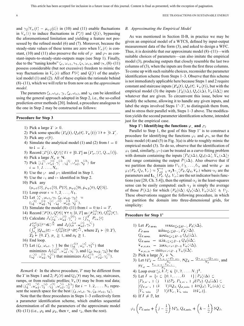
As was mentioned in Section II-B, in practice we may begiven an empirical model of a WTCS, defined by input-outputmeasurement data of the form (3), and asked to design a WFC.Thus, it is desirable that our approximate model (8)–(11)—withsuitable choices of parameters—can also imitate the empiricalmodel (3), producing outputs that closely resemble the last twocolumns of (3), when the inputs are from the first three columns.To come up with such suitable choices, reconsider the parameteridentification scheme from Steps 1–3. Observe that this schemeis not immediately applicable here because Steps 1 and 2 requireconstant and staircase inputs , but with theempirical model (3) the inputs arewhatever that are given. To circumvent this issue, below wemodify the scheme, allowing it to handle any given inputs, andlabel the steps involved Steps 1’–3’, to distinguish them from,and to stress their parallel with, Steps 1–3 above. The modifica-tion yields the second parameter identification scheme, intendedjust for the empirical case.Step 1’: Identifying the functions andParallel to Step 1, the goal of this Step 1’ is to construct a

procedure for identifying the functions and , so that thebasic model (4) and (5) in Fig. 3(a) is able to roughly mimic theempirical model (3). To do so, observe that the identification of(and, similarly, ) can be treated as a curve-fitting problem

with domain containing the inputsand range containing the output . Also observe that ifwe partition the domain into and write as

where are theparameters and are the set indicator basis func-tions (see [20, Ch. 5.4]), then the optimal in the least-squaressense can be easily computed: each is simply the averageof those for which .These observations suggest the following procedure, in whichwe partition the domain into three-dimensional grids, forsimplicity:

Procedure for Step 1’

1) Let

.2) Pick a large .3) Let , and


.6) If , let



where denotes the cardinality of .7) End loop.8) Determine and via interpolation on the (at most)

data points obtained.

Step 2’: Identifying the parameters andUnlike going from Step 1 to Step 1’ where the procedure

undergoes significant changes, only minor modifications areneeded to make the procedures in Steps 2 and 3 applicable tothe empirical model (3) in this Step 2’ and the next Step 3’. Inparticular, the inputs now come from the first three columns of(3), and now represent the desired norms, and andnow play the role of and in nullifying the impact of

the initial states:


1) Rename from the empirical model (3)as .

2) Pick a large .3) Pick and for .4) Use the and identified in Step 1’.5) Pick any .6) Loop over .7) Let and .8) Simulate the refined model (6) and (7) from to

.9) Record as

.

10) Calculate

and

, where

, and .11) End loop.12) Let , and

.

Step 3’: Identifying the parameters ,and


1) Rename from the empirical model (3)as .

2) Pick a large .

3) Pick for.

4) Use the and identified in Step 1’.5) Use the and identified in Step 2’.6) Pick any


.9) Simulate the approximate model (8)–(11) fromto .

10) Record as.

11) Calculate

where ,and .

12) End loop.13) Let be the that

minimizes , and be thethat minimizes .

Remark 5: The approximate model (8)–(11) in this sec-tion may be viewed as the WTCS in Section I, with

. Also, it maybe regarded as satisfying (C2) in Section I because it hasisolated static nonlinearities and is relatively simple comparedto full-blown WTCS models, such as those in Section IV.

IV. VALIDATION OF THE APPROXIMATE MODEL

In this section, we validate via simulation the approximatemodel developed in Section III, showing that it is capableof closely imitating several analytical and empirical WTCSmodels from the literature and from real data. To enable thevalidation, we first describe a wind turbine model, followedby the analytical and empirical WTCS models considered. Wethen describe the validation settings and results.

A. Wind Turbine Model

Consider a variable-speed wind turbine equipped with aDFIG.2 Under normal operating conditions, the turbine may bemodeled by the following differential and algebraic equations[16], [22]:

2Due to space limitation, only DFIG is considered in the model validation.Wenote, however, that other types of generators, such as IG, may be implementedin a similar manner.



where denote the stator and rotor; the frame;the fluxes; the volt-

ages; the currents; the resistances;the inductances; the

leakage coefficient; the constant angular velocity of thesynchronously rotating reference frame; the rotor angularvelocity; the rotor moment of inertia; the friction co-efficient; the mechanical torque;

the electromagnetic torque; the airdensity; the rotor swept area of radiusthe -surface; the tip speed ratio; and theblade pitch angle. In addition, to have some diversity in thevalidation, consider the following two distinct sets of values forthe wind turbine parameters: the first set of values is adoptedfrom [31], [32] and corresponds to a GE 3.6 MW turbine, whilethe second is adopted from MATLAB/Simulink R2007a andcorresponds to a GE 1.5 MW turbine. These two sets of valuesare listed in the Appendix.

B. WTCS Models

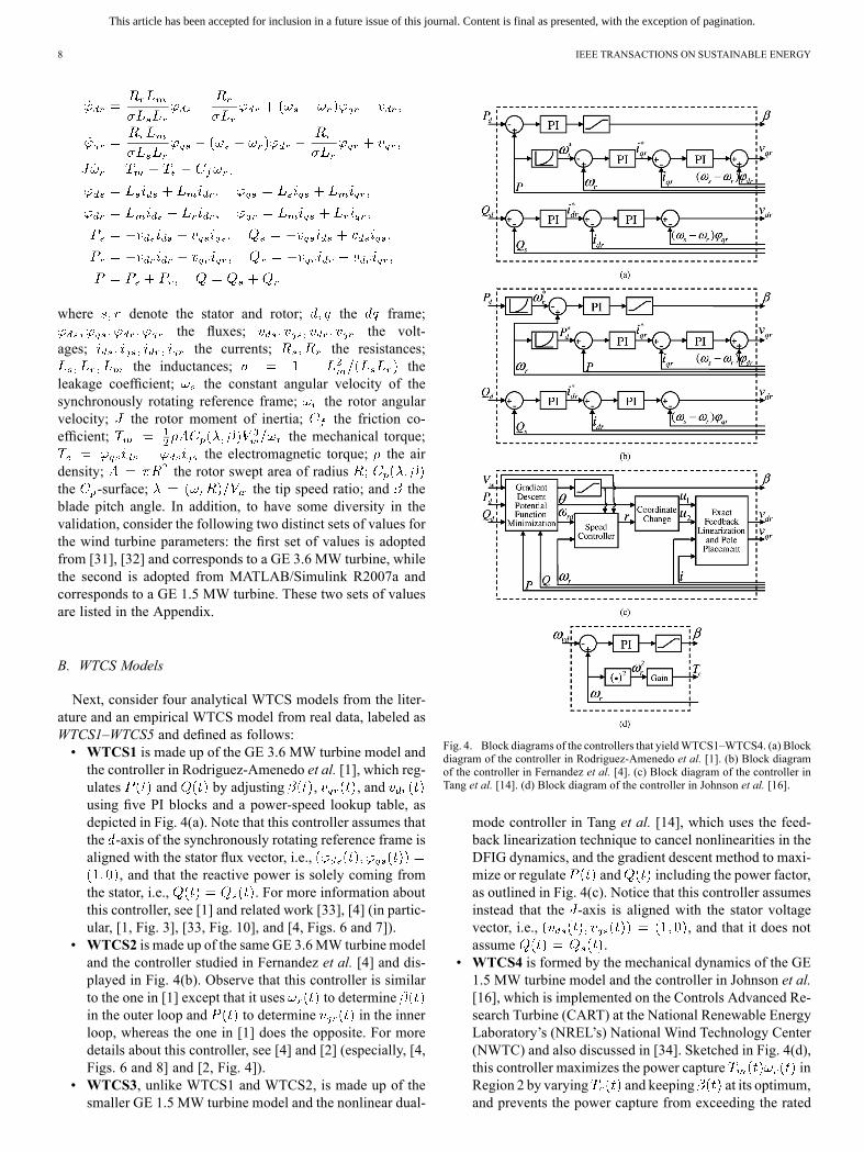
Next, consider four analytical WTCS models from the liter-ature and an empirical WTCS model from real data, labeled asWTCS1–WTCS5 and defined as follows:• WTCS1 is made up of the GE 3.6 MW turbine model andthe controller in Rodriguez-Amenedo et al. [1], which reg-ulates and by adjusting , , andusing five PI blocks and a power-speed lookup table, asdepicted in Fig. 4(a). Note that this controller assumes thatthe -axis of the synchronously rotating reference frame isaligned with the stator flux vector, i.e.,

, and that the reactive power is solely coming fromthe stator, i.e., . For more information aboutthis controller, see [1] and related work [33], [4] (in partic-ular, [1, Fig. 3], [33, Fig. 10], and [4, Figs. 6 and 7]).

• WTCS2 is made up of the same GE 3.6MW turbine modeland the controller studied in Fernandez et al. [4] and dis-played in Fig. 4(b). Observe that this controller is similarto the one in [1] except that it uses to determinein the outer loop and to determine in the innerloop, whereas the one in [1] does the opposite. For moredetails about this controller, see [4] and [2] (especially, [4,Figs. 6 and 8] and [2, Fig. 4]).

• WTCS3, unlike WTCS1 and WTCS2, is made up of thesmaller GE 1.5 MW turbine model and the nonlinear dual-

Fig. 4. Block diagrams of the controllers that yieldWTCS1–WTCS4. (a) Blockdiagram of the controller in Rodriguez-Amenedo et al. [1]. (b) Block diagramof the controller in Fernandez et al. [4]. (c) Block diagram of the controller inTang et al. [14]. (d) Block diagram of the controller in Johnson et al. [16].

mode controller in Tang et al. [14], which uses the feed-back linearization technique to cancel nonlinearities in theDFIG dynamics, and the gradient descent method to maxi-mize or regulate and including the power factor,as outlined in Fig. 4(c). Notice that this controller assumesinstead that the -axis is aligned with the stator voltagevector, i.e., , and that it does notassume .

• WTCS4 is formed by the mechanical dynamics of the GE1.5 MW turbine model and the controller in Johnson et al.[16], which is implemented on the Controls Advanced Re-search Turbine (CART) at the National Renewable EnergyLaboratory’s (NREL’s) National Wind Technology Center(NWTC) and also discussed in [34]. Sketched in Fig. 4(d),this controller maximizes the power capture inRegion 2 by varying and keeping at its optimum,and prevents the power capture from exceeding the rated



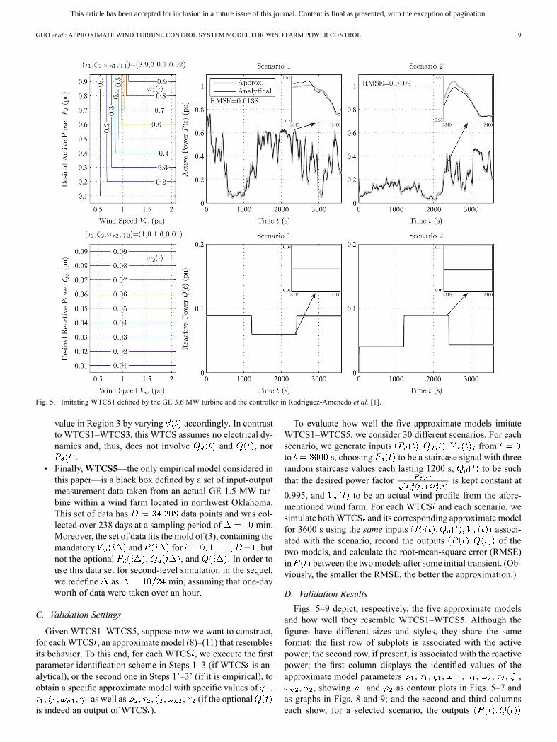
Fig. 5. Imitating WTCS1 defined by the GE 3.6 MW turbine and the controller in Rodriguez-Amenedo et al. [1].

value in Region 3 by varying accordingly. In contrastto WTCS1–WTCS3, this WTCS assumes no electrical dy-namics and, thus, does not involve and , nor

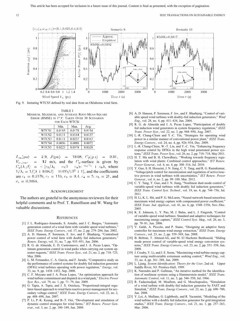
.• Finally,WTCS5—the only empirical model considered inthis paper—is a black box defined by a set of input-outputmeasurement data taken from an actual GE 1.5 MW tur-bine within a wind farm located in northwest Oklahoma.This set of data has data points and was col-lected over 238 days at a sampling period of min.Moreover, the set of data fits the mold of (3), containing themandatory and for , butnot the optional , , and . In order touse this data set for second-level simulation in the sequel,we redefine as min, assuming that one-dayworth of data were taken over an hour.

C. Validation Settings

Given WTCS1–WTCS5, suppose now we want to construct,for eachWTCS , an approximate model (8)–(11) that resemblesits behavior. To this end, for each WTCS , we execute the firstparameter identification scheme in Steps 1–3 (if WTCS is an-alytical), or the second one in Steps 1’–3’ (if it is empirical), toobtain a specific approximate model with specific values of ,, , , as well as , , , , (if the optional

is indeed an output of WTCS ).

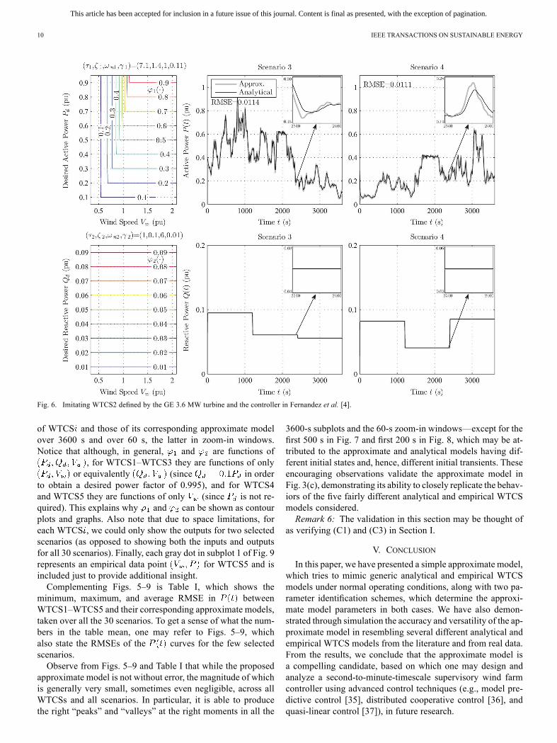
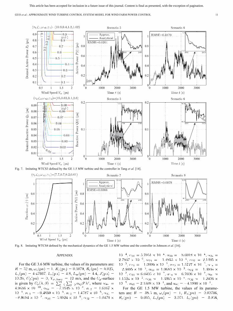
To evaluate how well the five approximate models imitateWTCS1–WTCS5, we consider 30 different scenarios. For eachscenario, we generate inputs fromto s, choosing to be a staircase signal with threerandom staircase values each lasting 1200 s, to be suchthat the desired power factor is kept constant at

0.995, and to be an actual wind profile from the afore-mentioned wind farm. For each WTCS and each scenario, wesimulate bothWTCS and its corresponding approximate modelfor 3600 s using the same inputs associ-ated with the scenario, record the outputs of thetwo models, and calculate the root-mean-square error (RMSE)in between the twomodels after some initial transient. (Ob-viously, the smaller the RMSE, the better the approximation.)

D. Validation Results

Figs. 5–9 depict, respectively, the five approximate modelsand how well they resemble WTCS1–WTCS5. Although thefigures have different sizes and styles, they share the sameformat: the first row of subplots is associated with the activepower; the second row, if present, is associated with the reactivepower; the first column displays the identified values of theapproximate model parameters , , , , , , , ,

, , showing and as contour plots in Figs. 5–7 andas graphs in Figs. 8 and 9; and the second and third columnseach show, for a selected scenario, the outputs



Fig. 6. Imitating WTCS2 defined by the GE 3.6 MW turbine and the controller in Fernandez et al. [4].

of WTCS and those of its corresponding approximate modelover 3600 s and over 60 s, the latter in zoom-in windows.Notice that although, in general, and are functions of

, for WTCS1–WTCS3 they are functions of onlyor equivalently (since in order

to obtain a desired power factor of 0.995), and for WTCS4and WTCS5 they are functions of only (since is not re-quired). This explains why and can be shown as contourplots and graphs. Also note that due to space limitations, foreach WTCS , we could only show the outputs for two selectedscenarios (as opposed to showing both the inputs and outputsfor all 30 scenarios). Finally, each gray dot in subplot 1 of Fig. 9represents an empirical data point for WTCS5 and isincluded just to provide additional insight.Complementing Figs. 5–9 is Table I, which shows the

minimum, maximum, and average RMSE in betweenWTCS1–WTCS5 and their corresponding approximate models,taken over all the 30 scenarios. To get a sense of what the num-bers in the table mean, one may refer to Figs. 5–9, whichalso state the RMSEs of the curves for the few selectedscenarios.Observe from Figs. 5–9 and Table I that while the proposed

approximate model is not without error, the magnitude of whichis generally very small, sometimes even negligible, across allWTCSs and all scenarios. In particular, it is able to producethe right “peaks” and “valleys” at the right moments in all the

3600-s subplots and the 60-s zoom-in windows—except for thefirst 500 s in Fig. 7 and first 200 s in Fig. 8, which may be at-tributed to the approximate and analytical models having dif-ferent initial states and, hence, different initial transients. Theseencouraging observations validate the approximate model inFig. 3(c), demonstrating its ability to closely replicate the behav-iors of the five fairly different analytical and empirical WTCSmodels considered.Remark 6: The validation in this section may be thought of

as verifying (C1) and (C3) in Section I.

V. CONCLUSION

In this paper, we have presented a simple approximate model,which tries to mimic generic analytical and empirical WTCSmodels under normal operating conditions, along with two pa-rameter identification schemes, which determine the approxi-mate model parameters in both cases. We have also demon-strated through simulation the accuracy and versatility of the ap-proximate model in resembling several different analytical andempirical WTCS models from the literature and from real data.From the results, we conclude that the approximate model isa compelling candidate, based on which one may design andanalyze a second-to-minute-timescale supervisory wind farmcontroller using advanced control techniques (e.g., model pre-dictive control [35], distributed cooperative control [36], andquasi-linear control [37]), in future research.



Fig. 7. Imitating WTCS3 defined by the GE 1.5 MW turbine and the controller in Tang et al. [14].

Fig. 8. Imitating WTCS4 defined by the mechanical dynamics of the GE 1.5 MW turbine and the controller in Johnson et al. [16].

APPENDIX

For the GE 3.6 MW turbine, the values of its parameters are:m,

m/s, and the -surfaceis given by , where , and .

For the GE 1.5 MW turbine, the values of its parame-ters are: m,



Fig. 9. Imitating WTCS5 defined by real data from an Oklahoma wind farm.

TABLE IMINIMUM, MAXIMUM, AND AVERAGE ROOT-MEAN-SQUAREERROR (RMSE) IN TAKEN OVER 30 SCENARIOS

FOR EACH WTCS

m/s, and the -surface is given by, where

, and the coefficientsare , and

.

ACKNOWLEDGMENT

The authors are grateful to the anonymous reviewers for theirhelpful comments and to Prof. T. Runolfsson and W. Wang forvaluable discussions.

REFERENCES[1] J. L. Rodriguez-Amenedo, S. Arnalte, and J. C. Burgos, “Automatic

generation control of a wind farm with variable speed wind turbines,”IEEE Trans. Energy Convers., vol. 17, no. 2, pp. 279–284, Jun. 2002.

[2] A. D. Hansen, P. Sorensen, F. Iov, and F. Blaabjerg, “Centralisedpower control of wind farm with doubly fed induction generators,”Renew. Energy, vol. 31, no. 7, pp. 935–951, Jun. 2006.

[3] R. G. de Almeida, E. D. Castronuovo, and J. A. Pecas Lopes, “Op-timum generation control in wind parks when carrying out system op-erator requests,” IEEE Trans. Power Syst., vol. 21, no. 2, pp. 718–725,May 2006.

[4] L. M. Fernandez, C. A. Garcia, and F. Jurado, “Comparative study onthe performance of control systems for doubly fed induction generator(DFIG) wind turbines operating with power regulation,” Energy, vol.33, no. 9, pp. 1438–1452, Sep. 2008.

[5] C. F. Moyano and J. A. Pecas Lopes, “An optimization approach forwind turbine commitment and dispatch in a wind park,” Electric PowerSyst. Res., vol. 79, no. 1, pp. 71–79, Jan. 2009.

[6] G. Tapia, A. Tapia, and J. X. Ostolaza, “Proportional-integral regu-lator-based approach to wind farm reactive power management for sec-ondary voltage control,” IEEE Trans. Energy Convers., vol. 22, no. 2,pp. 488–498, Jun. 2007.

[7] P. Li, P.-K. Keung, and B.-T. Ooi, “Development and simulation ofdynamic control strategies for wind farms,” IET Renew. Power Gen-erat., vol. 3, no. 2, pp. 180–189, Jun. 2009.

[8] A. D. Hansen, P. Sorensen, F. Iov, and F. Blaabjerg, “Control of vari-able speed wind turbines with doubly-fed induction generators,”WindEng., vol. 28, no. 4, pp. 411–434, Jun. 2004.

[9] R. G. de Almeida and J. A. Pecas Lopes, “Participation of doublyfed induction wind generators in system frequency regulation,” IEEETrans. Power Syst., vol. 22, no. 3, pp. 944–950, Aug. 2007.

[10] L.-R. Chang-Chien and Y.-C. Yin, “Strategies for operating windpower in a similar manner of conventional power plant,” IEEE Trans.Energy Convers., vol. 24, no. 4, pp. 926–934, Dec. 2009.

[11] L.-R. Chang-Chien, W.-T. Lin, and Y.-C. Yin, “Enhancing frequencyresponse control by DFIGs in the high wind penetrated power sys-tems,” IEEE Trans. Power Syst., vol. 26, no. 2, pp. 710–718,May 2011.

[12] H. T. Ma and B. H. Chowdhury, “Working towards frequency regu-lation with wind plants: Combined control approaches,” IET Renew.Power Generat., vol. 4, no. 4, pp. 308–316, Jul. 2010.

[13] Y. Guo, S. H. Hosseini, J. N. Jiang, C. Y. Tang, and R. G. Ramakumar,“Voltage/pitch control for maximization and regulation of active/reac-tive powers in wind turbines with uncertainties,” IET Renew. PowerGenerat., vol. 6, no. 2, pp. 99–109, Mar. 2012.

[14] C. Y. Tang, Y. Guo, and J. N. Jiang, “Nonlinear dual-mode control ofvariable-speed wind turbines with doubly fed induction generators,”IEEE Trans. Control Syst. Technol., vol. 19, no. 4, pp. 744–756, Jul.2011.

[15] H. Li, K. L. Shi, and P. G. McLaren, “Neural-network-based sensorlessmaximum wind energy capture with compensated power coefficient,”IEEE Trans. Ind. Applicat., vol. 41, no. 6, pp. 1548–1556, Nov./Dec.2005.

[16] K. E. Johnson, L. Y. Pao, M. J. Balas, and L. J. Fingersh, “Controlof variable-speed wind turbines: Standard and adaptive techniques formaximizing energy capture,” IEEE Control Syst. Mag., vol. 26, no. 3,pp. 70–81, Jun. 2006.

[17] V. Galdi, A. Piccolo, and P. Siano, “Designing an adaptive fuzzycontroller for maximum wind energy extraction,” IEEE Trans. EnergyConvers., vol. 23, no. 2, pp. 559–569, Jun. 2008.

[18] B. Beltran, T. Ahmed-Ali, and M. El Hachemi Benbouzid, “Slidingmode power control of variable-speed wind energy conversion sys-tems,” IEEE Trans. Energy Convers., vol. 23, no. 2, pp. 551–558, Jun.2008.

[19] J. Creaby, Y. Li, and J. E. Seem, “Maximizing wind turbine energy cap-ture using multivariable extremum seeking control,” Wind Eng., vol.33, no. 4, pp. 361–388, Jun. 2009.

[20] L. Ljung, System Identification: Theory for the User, 2nd ed. UpperSaddle River, NJ: Prentice-Hall, 1999.

[21] K. Narendra and P. Gallman, “An iterative method for the identifica-tion of nonlinear systems using a Hammerstein model,” IEEE Trans.Automatic Control, vol. 11, no. 3, pp. 546–550, Jul. 1966.

[22] R. Fadaeinedjad, M. Moallem, and G. Moschopoulos, “Simulationof a wind turbine with doubly-fed induction generator by FAST andSimulink,” IEEE Trans. Energy Convers., vol. 23, no. 2, pp. 690–700,Jun. 2008.

[23] Y. Lei, A. Mullane, G. Lightbody, and R. Yacamini, “Modeling of thewind turbine with a doubly fed induction generator for grid integrationstudies,” IEEE Trans. Energy Convers., vol. 21, no. 1, pp. 257–263,Mar. 2006.



[24] P. C. Krause, O. Wasynczuk, and S. D. Sudhoff, Analysis of ElectricMachinery and Drive Systems, 2nd ed. Piscataway, NJ: Wiley-IEEEPress, 2002.

[25] S. Frandsen, R. Barthelmie, S. Pryor, O. Rathmann, S. Larsen, J. Ho-jstrup, and M. Thogersen, “Analytical modelling of wind speed deficitin large offshore wind farms,” Wind Energy, vol. 9, no. 1, pp. 39–53,Jan. 2006.

[26] A. E. Feijoo and J. Cidras, “Modeling of wind farms in the load flowanalysis,” IEEE Trans. Power Syst., vol. 15, no. 1, pp. 110–115, Feb.2000.

[27] A. S. Dobakhshari and M. Fotuhi-Firuzabad, “A reliability model oflarge wind farms for power system adequacy studies,” IEEE Trans.Energy Convers., vol. 24, no. 3, pp. 792–801, Sep. 2009.

[28] M. Asmine, J. Brochu, J. Fortmann, R. Gagnon, Y. Kazachkov, C.-E.Langlois, C. Larose, E. Muljadi, J. MacDowell, P. Pourbeik, S. A.Seman, and K. Wiens, “Model validation for wind turbine generatormodels,” IEEE Trans. Power Syst., vol. 26, no. 3, pp. 1769–1782, Aug.2011.

[29] Standard Models for Variable Generation North American Electric Re-liability Corporation, Princeton, NJ, Special Report, 2010.

[30] M. Singh and S. Santoso, Dynamic Models for Wind Turbines andWind Power Plants National Renewable Energy Laboratory, Golden,CO, Subcontract Report, 2011.

[31] N. W. Miller, J. J. Sanchez-Gasca, W. W. Price, and R. W. Delmerico,“Dynamicmodeling of GE 1.5 and 3.6MWwind turbine-generators forstability simulations,” inProc. PESGeneralMeeting, Toronto, Canada,2003, pp. 1977–1983.

[32] W. Qiao, W. Zhou, J. M. Aller, and R. G. Harley, “Wind speed esti-mation based sensorless output maximization control for a wind tur-bine driving a DFIG,” IEEE Trans. Power Electron., vol. 23, no. 3, pp.1156–1169, May 2008.

[33] R. Pena, J. C. Clare, and G. M. Asher, “Doubly fed induction generatorusing back-to-back PWM converters and its application to variable-speed wind-energy generation,” IEE Proc. Electric Power Applicat.,vol. 143, no. 3, pp. 231–241, May 1996.

[34] L. Y. Pao and K. E. Johnson, “Control of wind turbines,” IEEE ControlSyst. Mag., vol. 31, no. 2, pp. 44–62, Apr. 2011.

[35] E. F. Camacho and C. B. Alba, Model Predictive Control, 2nd ed.London, England: Springer, 2007.

[36] J. Shamma, Cooperative Control of Distributed Multi-Agent Sys-tems. Chichester, England: Wiley, 2008.

[37] S. Ching, Y. Eun, C. Gokcek, P. T. Kabamba, and S. M. Meerkov,Quasilinear Control: Performance Analysis and Design of FeedbackSystems With Nonlinear Sensors and Actuators. New York: Cam-bridge Univ. Press, 2010.

Yi Guo (S’08) received the B.S. degree from TianjinPolytechnic University and the M.S. degree fromTianjin University, Tianjin, China, in 2002 and2005, respectively, and the Ph.D. degree in electricalengineering from the University of Oklahoma,Norman, in 2012.His current research interests include control

theory and applications, power system control andstability, and wind energy generation and integration.

S. Hossein Hosseini (S’10) received the B.S. degreefrom Sharif University of Technology, Tehran, Iran,in 2009. He is currently working toward the Ph.D.degree in the School of Electrical and Computer En-gineering at the University of Oklahoma, Norman.His current research interests include power

system economics and finance, and renewableenergy.

Choon Yik Tang (S’97–M’04) received the B.S. andM.S. degrees in mechanical engineering from Okla-homa State University, Stillwater, in 1996 and 1997,respectively, and the Ph.D. degree in electrical engi-neering from the University of Michigan, Ann Arbor,in 2003.He was a Postdoctoral Research Fellow in the

Department of Electrical Engineering and ComputerScience at the University of Michigan from 2003 to2004 and a Research Scientist at Honeywell Labs,Minneapolis, from 2004 to 2006. Since 2006, he

has been an Assistant Professor in the School of Electrical and ComputerEngineering, University of Oklahoma, Norman. His current research interestsinclude systems and control theory, distributed algorithms for computationand optimization over networks, control and operation of wind farms, andcomputationally efficient digital filter design.

John N. Jiang (SM’07) received the M.S. and Ph.D.degrees from the University of Texas at Austin.He is an Associate Professor in the Power System

Group in the School of Electrical and Computer En-gineering, University of Oklahoma, Norman. He hasbeen involved in a number of wind energy relatedprojects since 1989 in design, installation of stand-alone wind generation systems, the market impact ofwind generation in Texas, and recent large-scale windfarms development in Oklahoma.

Rama G. Ramakumar (M’62–SM’75–F’94–LF’02) received the B.E. degree from the Universityof Madras, Madras, India, the M.Tech. degree fromthe Indian Institute of Technology, Kharagpur, India,and the Ph.D. degree from Cornell University,Ithaca, NY, all in electrical engineering.After a decade (total) of service on the faculty of

the Coimbatore Institute of Technology, Coimbatore,India, he joined Oklahoma State University, Still-water, in 1967, where he has been a Professor since1976. In addition, he has been the Director of the

OSU Engineering Energy Laboratory since 1987. In 1991, he was named thePSO/Albrecht Naeter Professor of Electrical and Computer Engineering andwas promoted to Regents Professor in 2008. His research interests are in thearea of energy conversion, energy storage, power engineering, and renewableenergy. He has been a consultant to several national and supranational organi-zations in the field of energy and has organized and presented short courses onrenewable energy topics and engineering reliability. His contributions are doc-umented in over 150 publications, which include four U.S. patents, contributedchapters in four books and seven hand books, and technical papers in variousjournals, transactions, and national and international conference proceedings.He is the author of the text book Engineering Reliability Fundamentals andApplications (Englewood Cliffs, NY: Prentice-Hall, 1993).Dr. Ramakumar’s past and present leadership activities in the IEEE Power

and Energy Society include chairing the Awards Committee of the TechnicalCouncil, the award Subcommittee of the Power Engineering EducationCommittee, the Energy Development Subcommittee and the Renewable Tech-nologies Subcommittee of the Energy Development and Power GenerationCommittee, the Working Group on Renewable Technologies, and the FellowsWorking Group of the Power Engineering Education Committee. He is amember of the American and International Solar Energy Societies, the Amer-ican Society for Engineering Education, and the IEEE Industry ApplicationsSociety. He is a Registered Professional Engineer in the State of Oklahoma.

Documents

An Approximate Wind Turbine Control System Model for Wind Farm Power Control