An approximate Bayesian approach for quantitative trait loci estimation

Computational Statistics and Data Analysis 54 (2010) 565–574

Contents lists available at ScienceDirect

Computational Statistics and Data Analysis

journal homepage: www.elsevier.com/locate/csda

An approximate Bayesian approach for quantitative trait loci estimationYu-Ling Chang ∗, Fei Zou, Fred A. WrightDepartment of Biostatistics, University of North Carolina, Chapel Hill, NC 27599, United States

a r t i c l e i n f o

Article history:Received 27 October 2008Received in revised form 22 September2009Accepted 22 September 2009Available online 1 October 2009

a b s t r a c t

Bayesian approaches have been widely used in quantitative trait locus (QTL) linkageanalysis in experimental crosses, and have advantages in interpretability and inconstructing parameter probability intervals. Most existing Bayesian linkage methodsinvolve Monte Carlo sampling, which is computationally prohibitive for high-throughputapplications such as eQTL analysis. In this paper, we present a Bayesian linkage modelthat offers directly interpretable posterior densities or Bayes factors for linkage. For ourmodel, we employ the Laplace approximation for integration over nuisance parameters inbackcross (BC) and F2 intercross designs. Our approach is highly accurate, and very fastcompared with alternatives, including grid search integration, importance sampling, andMarkov Chain Monte Carlo (MCMC). Our approach is thus suitable for high-throughputapplications. Simulated and real datasets are used to demonstrate our proposed approach.

Published by Elsevier B.V.

1. Introduction

For the problem of mapping quantitative trait loci in experimental crosses, the interval mapping maximum likelihoodapproach of Lander and Botstein (1989) inspired a number of extensions, including regression approximations (Haley andKnott, 1992), composite interval mapping, multiple-QTL mapping (Jansen, 1993; Jansen and Stam, 1994; Zeng, 1993, 1994)and multiple interval mapping (Kao et al., 1999).The asymptotic results in Kong and Wright (1994) detailed non-standard behavior of maximum likelihood estimates

for QTL positions. Moreover, model selection remains a challenging and important aspect of linkage mapping, for whichstandard asymptotic approximations in traditional likelihood ratio testing may not work well (Lander and Botstein, 1989).These are among the reasons for the popularity of Bayesian QTL mapping methods, which have an advantage in producingposterior densities for all model parameters. However, most published Bayesian QTL approaches use Monte Carlo samplingof the parameter space (Satagopan et al., 1996; Berry, 1998; Sillanpaa and Arjas, 1998; Stephens and Fisch, 1998; Yi and Xu,2000, 2001; Yi, 2004; Huang et al., 2007), which is too slow for high-throughput applications in which the analysis mustbe repeated thousands of times. The model introduced here formally applies to the single-QTL setting (per phenotype), andextensions to the multiple QTL setting are underway. Nonetheless, our model has an immediate application to the analysisof expression quantitative trait loci (eQTL), in which tens of thousands of transcripts are analyzed as phenotypes for linkage(Schadt et al., 2003). Previous model-based eQTL methods are highly computational (Kendziorski et al., 2006), and BayesianeQTL approaches have been performed at only a few hundred marker positions (Gelfond et al., 2007). A computationallyefficient Bayesian eQTL approach would open up new avenues for research, enabling the flexible incorporation of priorbiological information, and is the subject of a separate manuscript.The present paper describes the mechanics of our approach in detail, which incorporates important simplifications in

the model and in integration over nuisance parameters. Our method has utility beyond eQTL analysis. For example, a fast

∗ Corresponding address: Office of Biostatistics, OTS/CDER, FDA, Silver Spring, MD, 20993, United States.E-mail addresses: [email protected], [email protected] (Y.-L. Chang), [email protected] (F. Zou), [email protected] (F.A. Wright).

0167-9473/$ – see front matter. Published by Elsevier B.V.doi:10.1016/j.csda.2009.09.029

http://www.elsevier.com/locate/csda

http://www.elsevier.com/locate/csda

mailto:[email protected]




http://dx.doi.org/10.1016/j.csda.2009.09.029

566 Y.-L. Chang et al. / Computational Statistics and Data Analysis 54 (2010) 565–574

Bayesian method can be used in sensitivity testing to various parameter settings. Other uses include empirical Bayesianmethods in which the posterior linkage probabilities are used to evaluate the likelihood for population hyperparameters,such as in meta-analyses of multiple experimental crosses.The major problem in linkage analysis concerns inference on the existence and position of a QTL. Bayesian QTL analysis

fundamentally involves integration over nuisance parameters, i.e., any parameters other than the QTL position itself. As aMonte Carlo alternative to MCMC, we may consider importance sampling of the posterior of the likelihood in the vicinity ofthe maximum likelihood estimate (m.l.e.). Noting that there are relatively few nuisance parameters in experimental crossmodels, it alsomay be reasonable to consider direct numerical integration, including grid search integration (Thisted, 1998).However, as we demonstrate in Results below, none of these approaches is practical for high-throughput applications.As a fundamentally different approach, we consider the shape of the likelihood in order to obtain an insight into the

problem. We note that the non-standard asymptotic behavior of the likelihood is confined to the QTL position estimate(Kong andWright, 1994). At a fixed putative position, the likelihood for the nuisance parameters typically follows regularityconditions for standard inference (Cox and Hinkley, 1974). As a consequence, integration over the nuisance parameters mayemploy the Laplace approximation (Daniels, 1954), which essentially involves approximating the likelihood by an unscaledmultivariate normal density. Integration then becomes equivalent to determining the scaling factor, for which we will usethem.l.e. and analytic derivations of the Fisher information. Thus the necessary computation is of the same order as standardLOD approaches. The Laplace approximation has been used to speed up an evaluation step in the MCMC method of Berry(1998), but otherwise has been largely overlooked in this setting.Here we employ the Laplace approximation to obtain the linkage posterior for backcross (BC) and F2 intercross data.

The backcross approach also applies to double haploid populations, and essentially applies to recombinant inbred data sets,albeitwith a higher effective recombination rate (Williams et al., 2001). For completeness,we provide comparisons toMCMCand alternative integration approaches as described above, demonstrating that the Laplace approximation is highly accurateand, due to its speed, uniquely suited for high-throughput applications. Simulations indicate that the advantages hold overa wide range of sample sizes, heritability, and other conditions. We further illustrate our approach by analyzing a real F2mouse dataset for plasma HDL cholesterol concentration (HDL) (Ishimori et al., 2004).

2. Methods

Throughout this paper we use the normal linear phenotype model commonly applied to quantitative trait data (Landerand Botstein, 1989). However, the general approach is applicable to a wide variety of parametric phenotypemodels, and thevast majority of QTL models fall within the exponential family (Wright and Kong, 1997).Let yi denote the phenotype for the ith individual. For a BC individual, we have the model

yi = µ+ a · gi(x)+ εi, (1)

where a is the QTL effect; x signifies the location of the QTL; gi(.) is a numerical representation of the genotype for the ithindividual at each position, and εi is the residual error, distributed N(0, σ 2). We code gi(.) as 1 or−1, according to whetherthe genotype at each position is BB (homozygote) or Bb (heterozygote). We use β = µ, a, σ 2 to represent the nuisanceparameters, occupying a possibly finite regionΩ for which the prior p(β) > 0. We wish to obtain the posterior probabilitythat the QTL is at position x, given data consisting of phenotypes y and marker genotype data g ,

p(x|data) =p(x)p(data|x)p(data)

=p(x)

∫Ωp(data,β|x)dβp(data)

=p(x)

∫Ωp(β)p(data|x,β)dβp(data)

. (2)

This prior is intentionally flexible, as for future applications it might be sensible to consider prior information fromprevious studies, or to place mass only on the genomic positions of genes, implicitly favoring gene-rich genomic regions.Our goal is to enable direct probability statements for the posterior of x at each position, so that the posterior for entireregions/chromosomes may be obtained via summation or integration. In contrast, numerous Bayesian QTL methods areinherently dependent on Bayes Factors (Kass and Raftery, 1995), for inference, for which evaluation of the evidence is lessformal. Nonetheless, Bayes Factors may also be easily obtained from our approach (see Discussion).The right-hand side of Eq. (2) follows from the assumption of independence of QTL position and effect size, p(x,β) =

p(x) p(β). We will denote the marker positions by the vector xm, and the markers flanking x by xleft, xright. The quantityp(data|x,β) is the ordinary interval mapping likelihood for n individuals:

p(data|x,β) = p(g(xm)

) n∏i=1

[ ∑k=−1,1

p(yi|gi(x) = k, x,β, gi(xleft), gi(xright)

)p(gi(x) = k|gi(xleft), gi(xright)

)], (3)

for which we use model (1) and Haldane’s map function for the genotype probabilities given the markers.Thus far, our presentation is simply a standard Bayesian outline of the problem. In contrast to other Bayesian QTL

approaches (Satagopan et al., 1996), however, we state the null hypothesis in terms of the QTL position x. If x is on the

Y.-L. Chang et al. / Computational Statistics and Data Analysis 54 (2010) 565–574 567

chromosome or chromosomes under study, the alternative hypothesis holds (i.e., HA : x < ∞). Otherwise, the nullhypothesis holds, which we denote H0: x = ∞ (Doerge et al., 1997). The more commonly-used form of null hypothesis,dating at least to Lander and Botstein (1989), is a no-gene null specified in terms of the nuisance parameters as β ∈ Ω0 ⊂ Ω .The latter approach enables pointwise significance testing to follow standard likelihood ratio approximations in nestedmodels (Lander and Botstein, 1989). However, in a Bayesian setting there is no inherent reason to favor this specification.Note that our null hypothesis can accommodate the situation where no gene exists - as the sample size increases, evidencewill accrue that the effect size is negligibly small. In practical terms, for likelihood ratio testing the two forms of nullhypotheses may be very similar, as the maximum null likelihood often represents a similar fit to the data using either form.An exception occurs when a QTL with large effect is present on a chromosome other than the one under study, causing abimodal phenotype distribution. Indeed, this situation is examined in Lander and Botstein (1989) as an example where theno-gene specification produces poor inference. However, this situation presents no conceptual difficulty for our approach,because the possibility is explicitly considered that an unobserved QTLmay produce such a phenotypemixture distribution.A second and important advantage to our null hypothesis specification is that the inference for x will be relatively

insensitive to the prior for β, because p(β) appears in both null and alternative terms in p(data). In contrast, when usingthe no-gene null hypothesis, inference can be highly sensitive to the prior for β, where the subspace Ω0 would typicallybe of lower dimension than Ω (see comment by van de Ven (2004) on the application of reversible-jump MC proceduresto handle this issue). We use a flat (proper) prior in our illustrations of the Bayesian approach, p(β) = 1

|Ω|. Thus Ω must

technically be finite. However, we can letΩ get arbitrarily large, approaching the result for an improper flat prior.Using the assumed prior for β, the integral in the numerator of Eq. (2) becomes∫

Ω

p(β)p(data|x,β)dβ =1|Ω|

∫Ω

p(data|x,β)dβ =1|Ω|C(x), (4)

where C(x) is the integrated likelihood for a fixed x. The denominator of Eq. (2) is

p(data) =∫x′p(x′)

∫Ω

p(β)p(data|x′,β)dβdx′ =

1|Ω|

∫x′p(x′)C(x′)dx′, (5)

so the 1|Ω|term cancels out in numerator and denominator. We obtain

p(x|data) =p(x)C(x)∫

x′ p(x′)C(x′)dx′

=p(x)C(x)∫

x′<∞ p(x′)C(x′)dx′ + p(∞)C(∞)

, (6)

where the denominator is partitioned into HA and H0 portions, and p(∞) is the prior for H0.For notational simplicity, we use integral notation for computingmarginals over x positions, although in practice this will

involve either integration or summation, as appropriate to the prior on x. Note that Eq. (6) neatly decomposes the posteriorinto p(x) and C(x) terms. Thus if the prior p(x) is changed or updated from external sources, the posterior may be easilycomputed with no need to recompute C(x). In this paper, we will use a discrete uniform p(x) over a grid with respect togenetic map position. However, this choice of prior entails no loss of generality.Finally, it simply remains to obtain C(x) for each x, including the null value C(∞). No analytic solution is available,

and we will use the results of a numerical grid search as the gold standard, to which we compare our proposed Laplaceapproximation, as well as a crude version of the Laplace approximation that is even more computationally efficient. Forcompleteness, we also examine alternate methods for evaluating the integral, including importance sampling and Markovchain Monte Carlo (MCMC) sampling.

2.1. The Laplace approximation

We focus on a single chromosome, with H0 : x = ∞ corresponding to the hypothesis that the QTL is unlinkedto the chromosome (although the approach is just as easily applied to an entire genome scan). For fixed x, we definef (β) = p(data|x,β). The applicability of the Laplace approximation relies on standard behavior for the log-likelihoodfor large sample sizes: the function is continuous, unimodal, twice differentiable, with a maximum in the interior of Ω(Azevedo-Filho and Shachter, 1994). The Laplace approximation can be motivated by a Taylor expansion at β for a fixed x:

log(f (β)) = log(f (β))−12(β − β)T Σ−1(β − β)+ O(‖β − β‖3). (7)

The m.l.e. β may be obtained using a standard maximization routine such as E-M, as is routinely performed in standardinterval mapping. Σ = I−1(β) is obtained by inverting the analytically-derived information matrix at β, although theobserved information may also be used. After exponentiating both sides and integrating over β, we obtain

C(x) =∫β∈Ω

f (β)dβ ≈∫f (β)dβ ≈ f (β)(2π)dim(β)/2|Σ |1/2 ≡ C(x), (8)

where the indefinite integral assumes the spaceΩ is ‘‘large,’’ and the (2π)dim(β)/2|Σ |1/2 term arises from integration over amultivariate normal density withmean β and covariancematrix Σ . Finally, we substitute C(x) for C(x) in Eq. (6) for x <∞.


-2 -1 0 1 2

0.0

0.5

1.0

1.5

2.0

2.5

3.0

Sig

ma2

a

0.6 0.8 1.0 1.2 1.4

0.6

0.8

1.0

1.2

1.4

Sig

ma2

mu

(a) µ = 1. (b) a = 0.5.

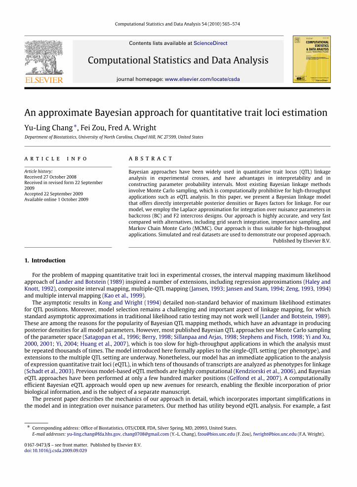
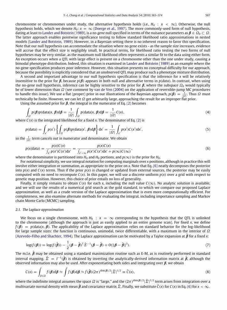
Fig. 1. Contour plot of Laplace Approximation for BC data under the null hypothesis: (a) n (sample size)= 100, µ = 1 (b) n (sample size)= 100, a = 0.5.

Our Laplace approximation is already very fast, but can be made even faster with a slight decrease in accuracy if theposterior tends to concentrate in a small genomic region. Under this scenario, we may replace |Σ(x)|1/2 by the singleestimate |Σ(x)|1/2 evaluated at the maximum posterior x location, because the uncertainty in β is nearly constant in theregion. We refer to this approach as our Laplace fixed approximation.

2.2. Approximating the null integrated likelihood

For the null value C(∞), the Laplace method may technically be applied, and will be asymptotically accurate. However,we have performed simulations demonstrating that the full Laplace approximation does not perform well under the nullhypothesis for realistic sample sizes when a true gene exists, but outside of the genomic region under study. Note that this isnot an inherent problem for the Bayesian approach, but affects the accuracy of the three-parameter Laplace approximation,which we will refer to as the naive null approximation. The difficulty is illustrated in Fig. 1(a), which shows likelihoodcontours for a, σ 2 under an assumedµ = 1 when n = 100, and the data represent a single simulation under the true nullmodelwith µ, a, σ 2 = 0, 1, 1. The null likelihood for one individual is amixture of twonormal densities,with each of thetwo genotype probabilities in Eq. (3) replaced by 1/2. In addition to the curvature in the likelihood contours, the likelihoodcan remain relatively flat over regions of the parameter space near the maximum, and it is difficult to prescribe a parametertransformation that will make the likelihood approximately normal in shape. Furthermore, if such a transformation wereavailable, it would be non-linear, and difficult to transform back to integration over the originalΩ .One approach to this problemwould be to apply numerical integration overΩ . However, we have devised the following

approximation requiring integration over only one parameter, using the fact that the Laplace approximation for µ, σ 2works well for a fixed a (see Fig. 1(b) for an illustration). Define fa(µ, σ 2) = pa(data|x = ∞, µ, σ 2), and µa, σ 2a (obtainednumerically) as the conditional m.l.e.s for a fixed a, with the corresponding covariance matrix estimate Σa on the restrictedspace. We then have the improved null Laplace approximation

C(∞) =∫af (µa, σ 2a )2π |Σa|

1/2da. (9)

This improved null can be sped up with a further approximation. For fixed a, model (1) implies E(Y |a) = µ andσ 2 = var(Y |a) − a2. For small to moderate a, the values y are approximate normal, with approximate conditional m.l.e.sµa = y, σ 2a = s

2y(n−1)/n−a

2/4. Approximate variance terms in thematrixΣ are var(µa) = s2y/n, var(σ2a ) = 2s

4y/(n−1) and

covariances= 0. For larger a, we find empirically that the m.l.e. approximation continues to work well, and the covarianceof the sample means and variances remains zero (because the distribution of y is symmetric). Note that under these furtherapproximations the parameter covariance matrix no longer depends on a, and the approach is used in Eq. (9) and termedthe fast null Laplace approximation.Supplemental Figs. 1 and 2 show the accuracy of the BC null posterior estimates using the naive null, improved null,

and fast null approximations for simulations under the true null (supplemental Fig. 1) and under the true alternative(supplemental Fig. 2). The improved and fast null approximations are highly accurate, while the naive null approximationshows considerable deviation from the accurate results based on grid search integration.

2.3. Extension to F2 populations

The Laplace approximation for F2 populations is somewhat more complicated, but straightforward. The correspondingphenotype model is:

yi = µ+ a · gi(x)+ d · (1− |gi(x)|)+ εi, (10)

where a and d are the additive and dominance effects for the QTL; gi(.) = 1 for genotype BB at the corresponding position,0 for genotype Bb, and−1 for genotype bb; and x is the true QTL position. The likelihood for n individuals follows the same


Laplace vs. Grid Search

X

0 10 20 30 40 50 60

X

0 10 20 30 40 50 60

X

0 10 20 30 40 50 60

X

0 10 20 30 40 50 60

0.00

000

0.00

010

0.00

020

p(x|

data

)0.

0000

00.

0001

00.

0002

0

p(x|

data

)

0.00

000

0.00

010

0.00

020

p(x|

data

)0.

0000

00.

0001

00.

0002

0

p(x|

data

)

Laplace "Fixed"(LF) vs. Grid Search

Importance Sampling(IM) vs. Grid Search Markov chain Monte Carlo(MCMC) vs. Grid Search

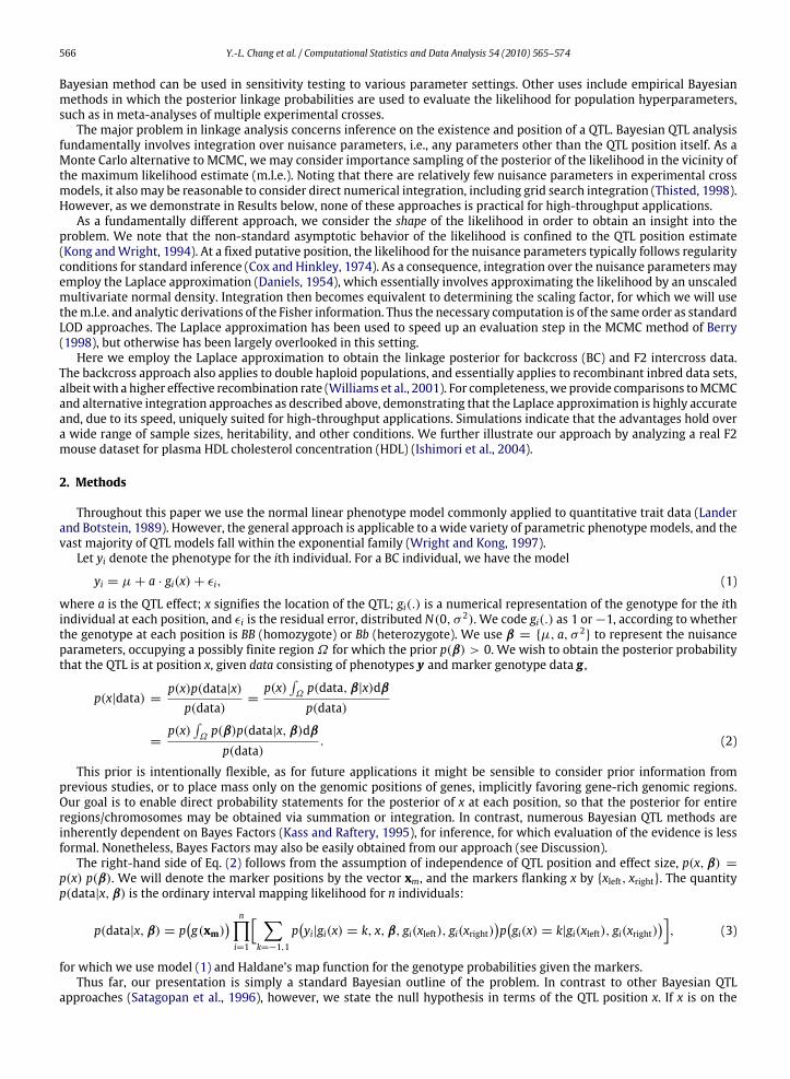
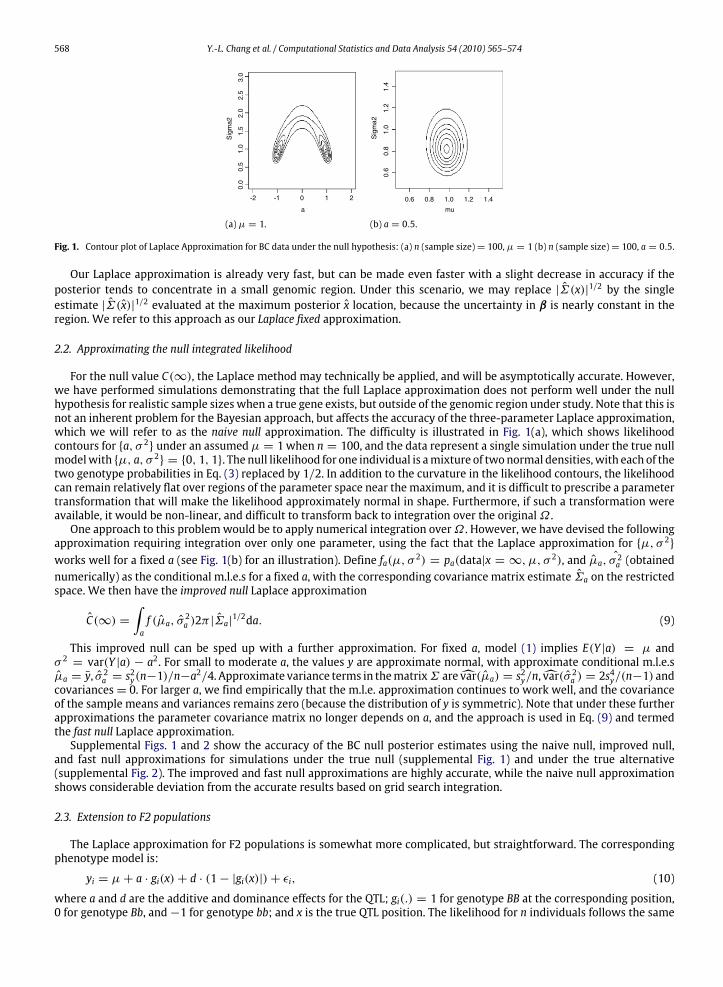
Fig. 2. Posterior distributions for BC data. Several methods are applied and compared with the grid search method (thin line).

form as Eq. (3), except that the summation is now over three genotypes, and the conditional genotype probabilities followthe form appropriate for F2 interval mapping (Lynch and Walsh, 1998).In order to estimate C(x) for F2 designs where x <∞, we directly apply the Laplace approximation as applied earlier to

Eq. (8), with β = µ, a, d, σ 2. In a similar manner to the null estimation for backcross individuals, the accurate estimationof C(∞) for F2 designs requires integration over both effect parameters a and d, with a Laplace approximation for theremaining parameters µ and σ 2.We have

C(∞) =∫ ∫ ∫ ∫

µ,a,d,σ 2L(µ, a, d, σ 2)dµdadddσ 2

≈ K∫ ∫

a,dfa,d(µa,d, σ 2a,d)dadd ≡ C(∞), (11)

where fa,d(µ, σ 2) = pa,d(data|x = ∞, µ, σ 2). Here K results from applying the fast null approximation heuristic usedearlier, modified for the F2 population: µa,d = y− d/2, σ 2a,d = s

2y − a

2/2− d2/4, and the contribution from the covariance

matrix yields K = π√

1n(n−1) (2s

2y)3/2. With the estimates of C(x) and C(∞) for the F2 sample, we finally obtain the

posterior probability p(x|data) for the Laplace approximation and the Laplace fixed approach. The accuracy of the F2 fastnull approximation is shown via simulations in supplemental Fig. 3, under both an example of a true null model and a truealternative model (supplemental Fig. 3).

3. Simulation studies

We conducted simulation studies for backcross (BC) and F2 intercross populations, respectively, to evaluate theperformance of our proposed methods and other existing methods. It is important to recognize that, although MCMCapproaches are typically used in Bayesian QTL mapping, our specification of the problem involves few enough parametersthat other approaches may be considered. Thus, for completeness, we examined several approaches.For numerical grid searches, we found that as few as 40 grid points for each nuisance parameter (20 for σ 2) gave highly

accurate results, as judged by additional investigations using finer grids. We thus view the grid search results as an effectivegold standard, keeping inmind that this grid density was already highly computationally intensive, and the empirical errors


0.00

0.05

0.10

0.15

X

p(x|

data

)

Laplace vs. Grid Search

0.00

0.05

0.10

0.15

p(x|

data

)

Laplace "Fixed"(LF) vs. Grid Search

0.00

0.05

0.10

0.15

p(x|

data

)

Importance Sampling(IM) vs. Grid Search

0.00

0.05

0.10

0.15

p(x|

data

)

Markov chain Monte Carlo(MCMC) vs. Grid Search

0 10 20 30 40 50 60

X

0 10 20 30 40 50 60

X

0 10 20 30 40 50 60

X

0 10 20 30 40 50 60

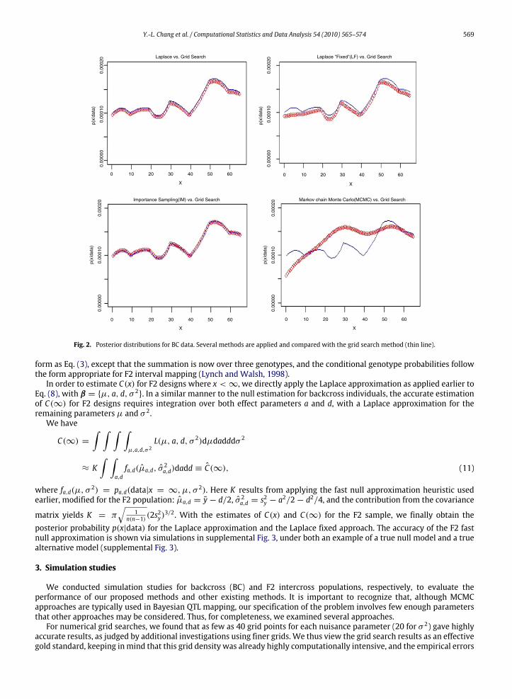
Fig. 3. Posterior distributions of QTL locations for the F2 data on chromosome 12 in Ishimori et al. (2004). Several methods are applied and compared withthe grid search method (thin line).

later observed in competing approaches far exceeded errors due to the choice of grid density. Integration was performed forµ, a, and d from−20/7 to 20/7 in increments of 1/7. For σ 2, the range of integration was 1/7 to 20/7 with increment 1/7.For the importance sampling approach, we specified proposal densities forµ, a and d as normal densities centered at the

MLEs and with standard deviations corresponding to the estimated standard errors. The proposal density of σ 2 was inversegamma(1, 1). We then used the ratios of the likelihoods to the proposal densities to obtain the numerical integral estimatewith 10,000 samples.The MCMC sampling procedure was standard (for examples in the QTL literature, see Satagopan et al. (1996) and Huang

et al. (2007)), and we burned in using the first 10,000 sweeps of the chain, and then performed an additional 100,000MCMCsweeps. The final samples were selected from every 100 sweeps to reduce serial correlation, resulting in 1000 samples fromthe posterior distribution. The approximated posterior distribution is calculated based on these samples. For simplicity, weemployed MCMC only for the alternative (i.e., x < ∞), using the grid search value for the null posterior. Our intent was topursue MCMC-based null calculations only if MCMC appeared to be computationally competitive. We did not include thenull computation time for MCMC in the results described below, and thus these MCMC results are more favorable than onewould encounter in practice.The simulation results below were performed using C on Linux PCs with Xeon 2.8 GHz processors.

3.1. BC QTL data

Our simulation studies for BC assumed a 100cM chromosome with at most one QTL. To generate the data, we simulatedmarker genotypes according to theHaldanemodel, and normally distributed phenotypeswithmeans determined by theQTLgenotype. Posterior probabilities were calculated at 1cM intervals, assuming a discrete uniform prior p(x) (which entails noloss in generality, as discussed earlier).Denoting the numerical grid search posterior as p(x|data) and each of the competing approaches as p(x|data), we

summarized the error by:∑x|p(x|data)− p(x|data)|

2, (12)


Table 1Speed(unit:second) when sample size= 200, QTL location= 45.1cM.

Methods Grid Search Laplace Laplace fixed IMS MCMC

Backcross

Heritability= 0Marker distance= 1cM 118.5856 0.0469 0.0401 3.5870 7.8091Marker distance= 5cM 118.1441 0.0536 0.0472 3.5785 7.2589Marker distance= 10cM 117.8861 0.0602 0.0538 3.9692 7.2077Marker distance= 20cM 117.4769 0.0707 0.0638 3.5848 7.1262

Heritability= 0.1Marker distance= 1cM 118.8081 0.0488 0.0417 3.5936 7.8286Marker distance= 5cM 117.8866 0.0563 0.0492 3.5757 7.2340Marker distance= 10cM 117.6759 0.0631 0.0569 3.5788 7.2318Marker distance= 20cM 117.4915 0.0753 0.0676 3.6003 7.1099

F2

Heritability= 0Marker distance= 1cM 1822.2490 0.3932 0.3762 12.6713 24.6592Marker distance= 5cM 1832.0760 0.4725 0.4506 12.7386 24.7834Marker distance= 10cM 2071.3200 0.4229 0.4074 14.4116 27.8797Marker distance= 20cM 1873.647 0.4503 0.4369 13.1088 25.3048

Heritability= 0.1Marker distance= 1cM 1827.2800 0.4131 0.3955 12.7035 24.7298Marker distance= 5cM 1831.5750 0.4963 0.4747 12.7495 24.8071Marker distance= 10cM 2070.4250 0.4444 0.4268 14.4784 27.9172Marker distance= 20cM 1875.3520 0.4708 0.4552 13.1258 25.2686

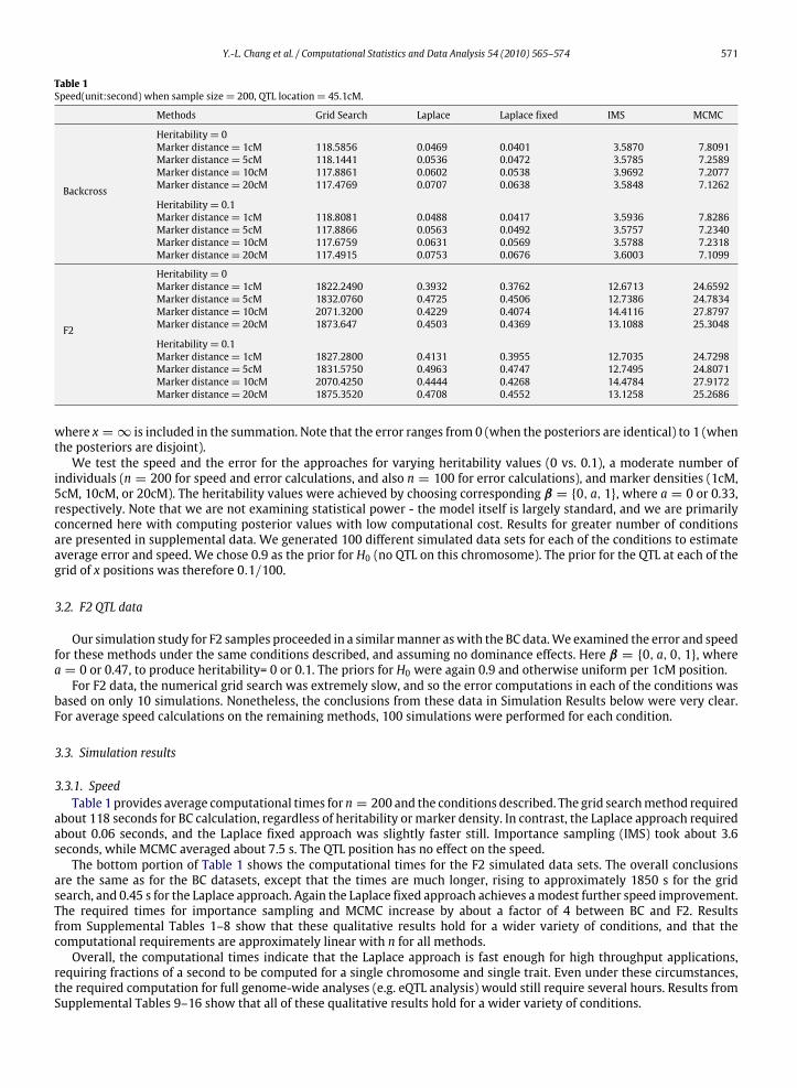
where x = ∞ is included in the summation. Note that the error ranges from 0 (when the posteriors are identical) to 1 (whenthe posteriors are disjoint).We test the speed and the error for the approaches for varying heritability values (0 vs. 0.1), a moderate number of

individuals (n = 200 for speed and error calculations, and also n = 100 for error calculations), and marker densities (1cM,5cM, 10cM, or 20cM). The heritability values were achieved by choosing corresponding β = 0, a, 1, where a = 0 or 0.33,respectively. Note that we are not examining statistical power - the model itself is largely standard, and we are primarilyconcerned here with computing posterior values with low computational cost. Results for greater number of conditionsare presented in supplemental data. We generated 100 different simulated data sets for each of the conditions to estimateaverage error and speed. We chose 0.9 as the prior for H0 (no QTL on this chromosome). The prior for the QTL at each of thegrid of x positions was therefore 0.1/100.

3.2. F2 QTL data

Our simulation study for F2 samples proceeded in a similarmanner aswith the BC data.We examined the error and speedfor these methods under the same conditions described, and assuming no dominance effects. Here β = 0, a, 0, 1, wherea = 0 or 0.47, to produce heritability= 0 or 0.1. The priors for H0 were again 0.9 and otherwise uniform per 1cM position.For F2 data, the numerical grid search was extremely slow, and so the error computations in each of the conditions was

based on only 10 simulations. Nonetheless, the conclusions from these data in Simulation Results below were very clear.For average speed calculations on the remaining methods, 100 simulations were performed for each condition.

3.3. Simulation results

3.3.1. SpeedTable 1 provides average computational times for n = 200 and the conditions described. The grid searchmethod required

about 118 seconds for BC calculation, regardless of heritability or marker density. In contrast, the Laplace approach requiredabout 0.06 seconds, and the Laplace fixed approach was slightly faster still. Importance sampling (IMS) took about 3.6seconds, while MCMC averaged about 7.5 s. The QTL position has no effect on the speed.The bottom portion of Table 1 shows the computational times for the F2 simulated data sets. The overall conclusions

are the same as for the BC datasets, except that the times are much longer, rising to approximately 1850 s for the gridsearch, and 0.45 s for the Laplace approach. Again the Laplace fixed approach achieves amodest further speed improvement.The required times for importance sampling and MCMC increase by about a factor of 4 between BC and F2. Resultsfrom Supplemental Tables 1–8 show that these qualitative results hold for a wider variety of conditions, and that thecomputational requirements are approximately linear with n for all methods.Overall, the computational times indicate that the Laplace approach is fast enough for high throughput applications,

requiring fractions of a second to be computed for a single chromosome and single trait. Even under these circumstances,the required computation for full genome-wide analyses (e.g. eQTL analysis) would still require several hours. Results fromSupplemental Tables 9–16 show that all of these qualitative results hold for a wider variety of conditions.


Table 2Error for backcross when QTL location= 45.1cM.

n Methods Laplace error LaplacefixedLaplace

IMSLaplace

MCMCLaplace

100

Heritability= 0Marker distance= 1cM 0.00106 2.61 2.97 11.90Marker distance= 5cM 0.00083 2.47 3.22 7.13Marker distance= 10cM 0.00109 2.82 3.55 6.43Marker distance= 20cM 0.00123 2.93 3.39 4.21

Heritability= 0.1Marker distance= 1cM 0.00451 3.53 3.72 24.56Marker distance= 5cM 0.00450 3.29 3.76 12.28Marker distance= 10cM 0.00452 3.11 3.55 9.77Marker distance= 20cM 0.00477 2.74 3.50 5.07

200



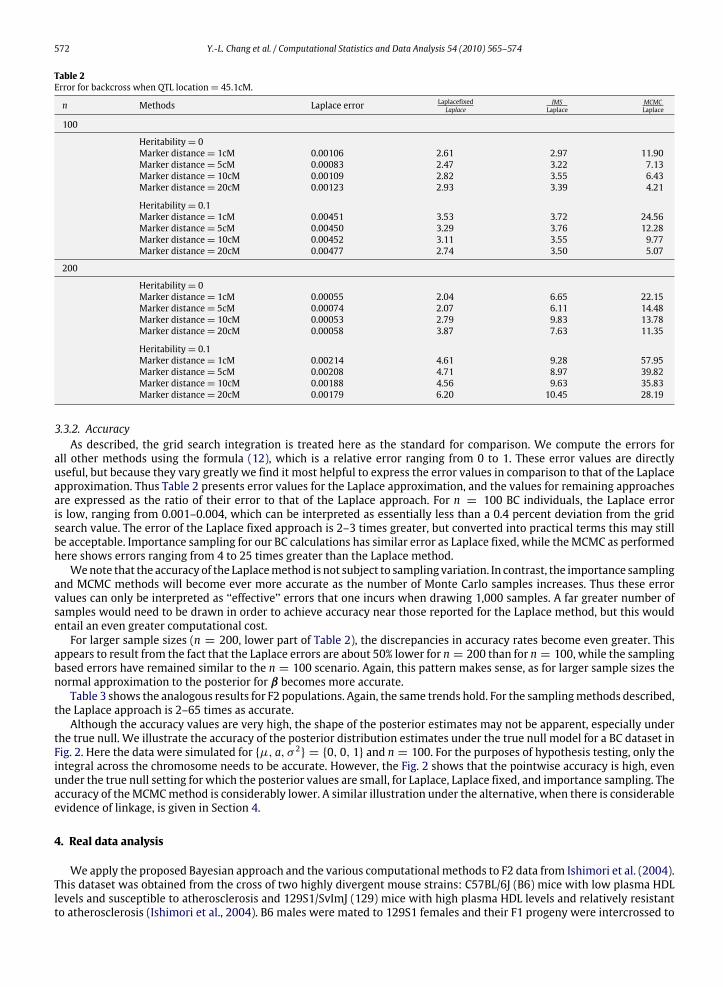
3.3.2. AccuracyAs described, the grid search integration is treated here as the standard for comparison. We compute the errors for

all other methods using the formula (12), which is a relative error ranging from 0 to 1. These error values are directlyuseful, but because they vary greatly we find it most helpful to express the error values in comparison to that of the Laplaceapproximation. Thus Table 2 presents error values for the Laplace approximation, and the values for remaining approachesare expressed as the ratio of their error to that of the Laplace approach. For n = 100 BC individuals, the Laplace erroris low, ranging from 0.001–0.004, which can be interpreted as essentially less than a 0.4 percent deviation from the gridsearch value. The error of the Laplace fixed approach is 2–3 times greater, but converted into practical terms this may stillbe acceptable. Importance sampling for our BC calculations has similar error as Laplace fixed, while theMCMC as performedhere shows errors ranging from 4 to 25 times greater than the Laplace method.Wenote that the accuracy of the Laplacemethod is not subject to sampling variation. In contrast, the importance sampling

and MCMC methods will become ever more accurate as the number of Monte Carlo samples increases. Thus these errorvalues can only be interpreted as ‘‘effective’’ errors that one incurs when drawing 1,000 samples. A far greater number ofsamples would need to be drawn in order to achieve accuracy near those reported for the Laplace method, but this wouldentail an even greater computational cost.For larger sample sizes (n = 200, lower part of Table 2), the discrepancies in accuracy rates become even greater. This

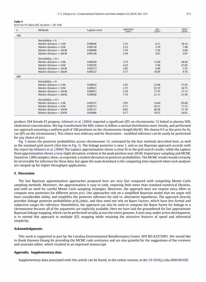
appears to result from the fact that the Laplace errors are about 50% lower for n = 200 than for n = 100, while the samplingbased errors have remained similar to the n = 100 scenario. Again, this pattern makes sense, as for larger sample sizes thenormal approximation to the posterior for β becomes more accurate.Table 3 shows the analogous results for F2 populations. Again, the same trends hold. For the samplingmethods described,

the Laplace approach is 2–65 times as accurate.Although the accuracy values are very high, the shape of the posterior estimates may not be apparent, especially under

the true null. We illustrate the accuracy of the posterior distribution estimates under the true null model for a BC dataset inFig. 2. Here the data were simulated for µ, a, σ 2 = 0, 0, 1 and n = 100. For the purposes of hypothesis testing, only theintegral across the chromosome needs to be accurate. However, the Fig. 2 shows that the pointwise accuracy is high, evenunder the true null setting for which the posterior values are small, for Laplace, Laplace fixed, and importance sampling. Theaccuracy of theMCMCmethod is considerably lower. A similar illustration under the alternative, when there is considerableevidence of linkage, is given in Section 4.

4. Real data analysis

We apply the proposed Bayesian approach and the various computational methods to F2 data from Ishimori et al. (2004).This dataset was obtained from the cross of two highly divergent mouse strains: C57BL/6J (B6) mice with low plasma HDLlevels and susceptible to atherosclerosis and 129S1/SvImJ (129) mice with high plasma HDL levels and relatively resistantto atherosclerosis (Ishimori et al., 2004). B6 males were mated to 129S1 females and their F1 progeny were intercrossed to


Table 3Error for F2 when QTL location= 45.1cM.

n Methods Laplace error LaplacefixedLaplace

IMSLaplace

MCMCLaplace

100



200



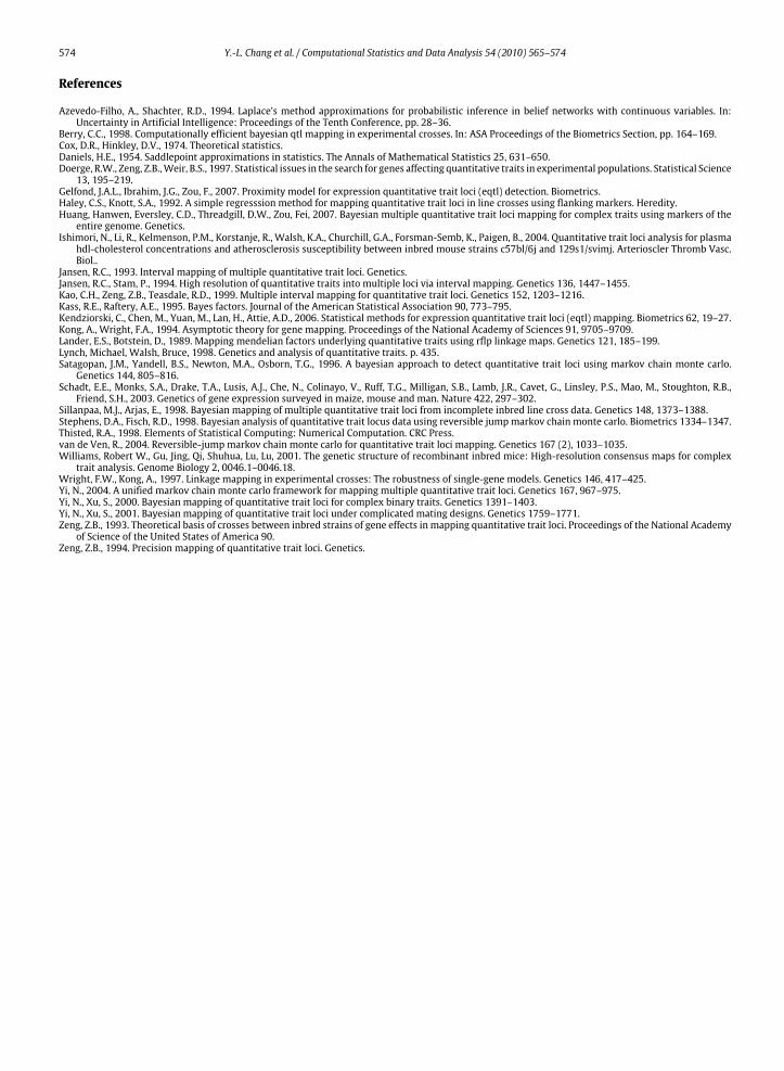
produce 294 female F2 progeny. Ishimori et al. (2004) reported a significant QTL on chromosome 12 linked to plasma HDLcholesterol concentration. We log-transformed the HDL values to follow a normal distribution more closely, and performedour approach assuming a uniform grid of 100 positions on the chromosome (length 66cM).We choose 0.5 as the prior forH0(no QTL on the chromosome). This choice was arbitrary and for illustration - modified inference can be easily be performedfor any choice of p(x).Fig. 3 shows the posterior probabilities across chromosome 12, estimated by the four methods described here, as well

as the standard grid search (thin line in Fig. 3). The linkage posterior is near 1, and so our Bayesian approach accords withthe report by Ishimori et al. (2004) The Laplace approximation shows a close fit to the grid search results, while the Laplacefixed approximation shows a very slight deviation, evident at the peak position near 20cM. Importance sampling andMCMC(based on 1,000 samples) show, as expected, amodest deviation in posterior probabilities. TheMCMC resultswould certainlybe serviceable for inference for these data, but again themain drawback is the computing time requiredwhen such analysesare ramped up for higher throughput applications.

5. Discussion

The fast Bayesian approximation approaches proposed here are very fast compared with competing Monte–Carlosampling methods. Moreover, the approximation is easy to code, requiring little more than standard numerical libraries,and with no need for careful Monte Carlo sampling strategies. Moreover, the approach does not require extra effort tocompute new posteriors for different priors p(x). Our approaches rely on a simplified Bayesian model that we argue willhave considerable utility, and simplifies the posterior inference for null vs. alternative hypotheses. The approach directlyprovides linkage posterior probabilities p(HA|data), and thus need not rely on Bayes Factors, which have less formal andsubjective ranges for inference. Nonetheless, the approach can also be used to compute the Bayes Factor for linkage to achromosome because all of the arguments are explicitly available. Here we have laid the groundwork for fast approximateBayesian linkagemapping,which can be performed serially across the entire genome. A next step, under active development,is to extend this approach to multiple QTL mapping while retaining the attractive features of speed and inferentialsimplicity.

Acknowledgments

This work is supported in part by the Carolina Environmental Bioinformatics Center, EPA RD-83272001. We would liketo thank Hanwen Huang for providing the MCMC code assistance and are also grateful for the suggestions of the reviewerand associate editor, which resulted in an improved manuscript.

Appendix. Supplementary data

Supplementary data associated with this article can be found, in the online version, at doi:10.1016/j.csda.2009.09.029.

http://dx.doi.org/doi:10.1016/j.csda.2009.09.029


References

Azevedo-Filho, A., Shachter, R.D., 1994. Laplace’s method approximations for probabilistic inference in belief networks with continuous variables. In:Uncertainty in Artificial Intelligence: Proceedings of the Tenth Conference, pp. 28–36.

Berry, C.C., 1998. Computationally efficient bayesian qtl mapping in experimental crosses. In: ASA Proceedings of the Biometrics Section, pp. 164–169.Cox, D.R., Hinkley, D.V., 1974. Theoretical statistics.Daniels, H.E., 1954. Saddlepoint approximations in statistics. The Annals of Mathematical Statistics 25, 631–650.Doerge, R.W., Zeng, Z.B.,Weir, B.S., 1997. Statistical issues in the search for genes affecting quantitative traits in experimental populations. Statistical Science13, 195–219.

Gelfond, J.A.L., Ibrahim, J.G., Zou, F., 2007. Proximity model for expression quantitative trait loci (eqtl) detection. Biometrics.Haley, C.S., Knott, S.A., 1992. A simple regresssion method for mapping quantitative trait loci in line crosses using flanking markers. Heredity.Huang, Hanwen, Eversley, C.D., Threadgill, D.W., Zou, Fei, 2007. Bayesian multiple quantitative trait loci mapping for complex traits using markers of theentire genome. Genetics.

Ishimori, N., Li, R., Kelmenson, P.M., Korstanje, R., Walsh, K.A., Churchill, G.A., Forsman-Semb, K., Paigen, B., 2004. Quantitative trait loci analysis for plasmahdl-cholesterol concentrations and atherosclerosis susceptibility between inbred mouse strains c57bl/6j and 129s1/svimj. Arterioscler Thromb Vasc.Biol..

Jansen, R.C., 1993. Interval mapping of multiple quantitative trait loci. Genetics.Jansen, R.C., Stam, P., 1994. High resolution of quantitative traits into multiple loci via interval mapping. Genetics 136, 1447–1455.Kao, C.H., Zeng, Z.B., Teasdale, R.D., 1999. Multiple interval mapping for quantitative trait loci. Genetics 152, 1203–1216.Kass, R.E., Raftery, A.E., 1995. Bayes factors. Journal of the American Statistical Association 90, 773–795.Kendziorski, C., Chen, M., Yuan, M., Lan, H., Attie, A.D., 2006. Statistical methods for expression quantitative trait loci (eqtl) mapping. Biometrics 62, 19–27.Kong, A., Wright, F.A., 1994. Asymptotic theory for gene mapping. Proceedings of the National Academy of Sciences 91, 9705–9709.Lander, E.S., Botstein, D., 1989. Mapping mendelian factors underlying quantitative traits using rflp linkage maps. Genetics 121, 185–199.Lynch, Michael, Walsh, Bruce, 1998. Genetics and analysis of quantitative traits. p. 435.Satagopan, J.M., Yandell, B.S., Newton, M.A., Osborn, T.G., 1996. A bayesian approach to detect quantitative trait loci using markov chain monte carlo.Genetics 144, 805–816.

Schadt, E.E., Monks, S.A., Drake, T.A., Lusis, A.J., Che, N., Colinayo, V., Ruff, T.G., Milligan, S.B., Lamb, J.R., Cavet, G., Linsley, P.S., Mao, M., Stoughton, R.B.,Friend, S.H., 2003. Genetics of gene expression surveyed in maize, mouse and man. Nature 422, 297–302.

Sillanpaa, M.J., Arjas, E., 1998. Bayesian mapping of multiple quantitative trait loci from incomplete inbred line cross data. Genetics 148, 1373–1388.Stephens, D.A., Fisch, R.D., 1998. Bayesian analysis of quantitative trait locus data using reversible jumpmarkov chain monte carlo. Biometrics 1334–1347.Thisted, R.A., 1998. Elements of Statistical Computing: Numerical Computation. CRC Press.van de Ven, R., 2004. Reversible-jump markov chain monte carlo for quantitative trait loci mapping. Genetics 167 (2), 1033–1035.Williams, Robert W., Gu, Jing, Qi, Shuhua, Lu, Lu, 2001. The genetic structure of recombinant inbred mice: High-resolution consensus maps for complextrait analysis. Genome Biology 2, 0046.1–0046.18.

Wright, F.W., Kong, A., 1997. Linkage mapping in experimental crosses: The robustness of single-gene models. Genetics 146, 417–425.Yi, N., 2004. A unified markov chain monte carlo framework for mapping multiple quantitative trait loci. Genetics 167, 967–975.Yi, N., Xu, S., 2000. Bayesian mapping of quantitative trait loci for complex binary traits. Genetics 1391–1403.Yi, N., Xu, S., 2001. Bayesian mapping of quantitative trait loci under complicated mating designs. Genetics 1759–1771.Zeng, Z.B., 1993. Theoretical basis of crosses between inbred strains of gene effects in mapping quantitative trait loci. Proceedings of the National Academyof Science of the United States of America 90.

Zeng, Z.B., 1994. Precision mapping of quantitative trait loci. Genetics.

Documents

An approximate Bayesian approach for quantitative trait loci estimation