Embed Size (px)
Citation preview
An Approach to Predict Operational Performance
of Airline Schedules Using Aircraft Assignment
Key Performance Indicators
by
Robin Riedel
Submitted to the Department of Aeronautics and Astronautics
in partial fulfillment of the requirements for the degree of
Master of Science in Aeronautics and Astronautics
at the
MASSACHUSETTS INSTITUTE OF TECHNOLOGY
June 2006
All rights reserved.@ Massachusetts Institute of Technology 2006.
A uthor ..........................Department of Aeronautics and Astronautics
May 22nd, 2006
Certified by ................ .,. .. . . ....... - -. - - -. ...i ...- -. - - - - -. .7
John-Paul B. ClarkePrincipal Research Scientist
Thesis SupervisorI
Accepted by ...............Jaime Peraire
Professor of Aeronautics and Astronautics
Chair, Committee on Graduate Students
AERO

2

An Approach to Predict Operational Performance of Airline
Schedules Using Aircraft Assignment Key Performance
Indicators
by
Robin Riedel
Submitted to the Department of Aeronautics and Astronauticson May 22nd, 2006, in partial fulfillment of the
requirements for the degree ofMaster of Science in Aeronautics and Astronautics
Abstract
This thesis presents an approach for predicting operational performance of airlineson the basis of flight schedules and aircraft assignments. The methodology usesaggregate measures of properties of aircraft assignments, called Aircraft AssignmentKey Performance Indicators (KPIs), and aims to find correlations between them andthe operational performance of the airline. A simulation experiment is prepared togather a large set of data points for analysis. A motivation is given for the use ofcontrol theoretic approaches in airline operations to utilize the KPIs as a basis forinitial planning and corrective actions.
Thesis Supervisor: John-Paul B. ClarkeTitle: Principal Research Scientist
3

4

Acknowledgments
There are a number of people who contributed to this work. I would like to express
my gratitude to
- my parents, grandparents and siblings for their support over the years I spent
at MIT.
- my thesis advisor, John-Paul Clarke, as well as all other participants in the
Airline KPI Project, especially Michel Turcotte at Air Canada, Erik Ander-
sson, Fredrik Johansson, Stefan Karisch, and Antonio Viegas Alves at Car-
men Systems, Gerrit Klempert, Christoph Klingenberg, Michael Mederer and
Brigitte Stolz at Lufthansa, and Terran Melconian, Praveen Pamidimukkala,
and Michelangelo Raimondi at MIT, for the productive and pleasant collabora-
tion.
- my friends and colleagues at MIT, especially Louis Breger, Nayden Kambouchev,
Georg Theis, and Laura Waller for their continuous support in preparing this
thesis.
- Cynthia Bernhart, David Darmofal, Amedeo Odoni, Jaime Peraire, Raul Radovitzky,
and David Robertson at MIT for their exceptional teaching and their integrity,
that made my time at MIT that much more enjoyable.
- Christian Kaufer for his continuous support of my flying career which I could
not have continued throughout graduate school otherwise.
5

6

Contents
1 Introduction 13
1.1 M otivation . . . . . . . . . . . . . . . . . . . . . . . . . . . . . . . . . 13
1.2 T hesis O utline . . . . . . . . . . . . . . . . . . . . . . . . . . . . . . . 15
2 Overview of Airline Scheduling, Operation, and Recovery 17
2.1 Airline Scheduling . . . . . . . . . . . . . . . . . . . . . . . . . . . . . 17
2.1.1 Flight Scheduling . . . . . . . . . . . . . . . . . . . . . . . . . 18
2.1.2 Aircraft Assignment . . . . . . . . . . . . . . . . . . . . . . . 20
2.1.3 Crew Scheduling . . . . . . . . . . . . . . . . . . . . . . . . . 22
2.2 Airline Operation . . . . . . . . . . . . . . . . . . . . . . . . . . . . . 23
2.3 Airline Recovery . . . . . . . . . . . . . . . . . . . . . . . . . . . . . 27
3 Key Performance Indicators and Output Measures 29
3.1 General Definitions . . . . . . . . . . . . . . . . . . . . . . . . . . . . 29
3.2 Aircraft Assignment Related Key Performance Indicators . . . . . . . 31
3.2.1 Fleet Assignment Buffer Statistics . . . . . . . . . . . . . . . . 31
3.2.2 Global Fleet Composition Indicators . . . . . . . . . . . . . . 35
3.2.3 Swap Option Indicators . . . . . . . . . . . . . . . . . . . . . 39
3.3 Output Measures . . . . . . . . . . . . . . . . . . . . . . . . . . . . . 42
3.3.1 Delay Minutes . . . . . . . . . . . . . . . . . . . . . . . . . . . 43
3.3.2 On-Time Performance . . . . . . . . . . . . . . . . . . . . . . 44
4 Application of Control Theory in Airline Operations 47
7

4.1 B ackground . . . . . . . . . . . . . . . . . . . . . . . . . . . . . . . .
4.2 Example of an Application of Control Theory in Airline Operations .
5 Simulation Setup
5.1 MIT Extensible Air Network Simulation
5.2 Integrated Operations Control System
5.3 Simulation Input . . . . . . . . . . . . .
5.3.1 Flight Schedules . . . . . . . . . .
5.3.2 Aircraft Assignments . . . . . . .
5.3.3 Taxi Times . . . . . . . . . . . .
5.3.4 Flight Times . . . . . . . . . . .
5.3.5 Airport Capacity Profiles . . . . .
5.3.6 Weather Scenarios . . . . . . . .
5.3.7 Airport Traffic . . . . . . . . . .
6 Proposed Analysis
6.1 Initial A nalysis . . . . . . . . . . . . . . . . . . . . . . . . . . . . . .
6.2 Optimization of Weighting Coefficients and Functions . . . . . . . . .
7 Directions for Future Research
A Acronyms and Initialisms
B Derivation of Probability Density Function of Flight Time
C Weather Scenarios
8
47
49
57
. . . . . . . . . . . . . . . . 57
. . . . . . . . . . . . . . . . 59
. . . . . . . . . . . . . . . . 60
. . . . . . . . . . . . . . . . 60
. . . . . . . . . . . . . . . . 60
. . . . . . . . . . . . . . . . 61
. . . . . . . . . . . . . . . . 63
. . . . . . . . . . . . . . . . 67
. . . . . . . . . . . . . . . . 69
. . . . . . . . . . . . . . . . 69
73
73
74
77
81
83
85

List of Figures
2-1 Parts of an Airline Schedule . . . . . . . . . . . . . . . . . . . . . . . 17
2-2 Time Terminology . . . . . . . . . . . . . . . . . . . . . . . . . . . . 18
2-3 Network Strategies . . . . . . . . . . . . . . . . . . . . . . . . . . . . 19
2-4 Example of Delay Propagation . . . . . . . . . . . . . . . . . . . . . . 24
2-5 On-Time Performance and Delay Causes by Number of Operations in
October 2005 (USA only) . . . . . . . . . . . . . . . . . . . . . . . . 25
2-6 Delay Causes by Delay Minutes in October 2005 (USA only) . . . . . 25
2-7 Original Delay Causes by Delay Minutes in October 2005 (USA only) 26
3-1 Temporal Relation of KPIs and the performance . . . . . . . . . . . . 30
3-2 Timeline of the Ground Process Between Two Flights . . . . . . . . 32
3-3 Example Buffer Weighting Functions . . . . . . . . . . . . . . . . . . 34
3-4 Timeline of Aircraft Arrivals and Departures . . . . . . . . . . . . . . 35
3-5 GFCI exam ples . . . . . . . . . . . . . . . . . . . . . . . . . . . . . . 37
3-6 Influence of Choice of Wf on GFCI . . . . . . . . . . . . . . . . . . . 38
3-7 Timeline of Ground Arcs of Aircraft of Different Fleet Types . . . . . 42
3-8 Example On-Blocks Delay Distribution and On-Time Performance . . 45
4-1 Control System Block Diagrams . . . . . . . . . . . . . . . . . . . . . 48
4-2 Airline Delay Control System . . . . . . . . . . . . . . . . . . . . . . 51
4-3 Response of the P-controlled System to a Change in DMPAdesired . . 52
4-4 Response of the System for Different Gain Values . . . . . . . . . . . 53
4-5 Response of the System to Constant Weather . . . . . . . . . . . . . 54
4-6 Response of the System to Random Weather . . . . . . . . . . . . . . 54
9

5-1 MEANS Modular Structure ...... ....................... 58
5-2 Taxi Time Distributions . . . . . . . . . . . . . . . . . . . . . . . . . 62
5-3 Example Flight Time Distributions . . . . . . . . . . . . . . . . . . . 64
5-4 Example Unimpeded Flight Time Distributions . . . . . . . . . . . . 65
5-5 Airport Capacity Profiles . . . . . . . . . . . . . . . . . . . . . . . . . 68
5-6 A irport Traffic . . . . . . . . . . . . . . . . . . . . . . . . . . . . . . . 71
6-1 Plot of Hypothetical Correlation between GSD and OTP . . . . . . . 75
10

List of Tables
2.1 Example Overview of an Airline's Maintenance System [3] . . . . . . 22
3.1 Properties of Aircraft for Example Airline . . . . . . . . . . . . . . . 38
5.1 W eather Categories [27] . . . . . . . . . . . . . . . . . . . . . . . . . 69
11

12

Chapter 1
Introduction
1.1 Motivation
Delays are an expected part of air travel today. Over the last seven years, approxi-
mately one fifth (21.5%) of all domestic flights in the United States of America (USA)
were either delayed' or canceled [22]. The situation in Europe is similar [11]. A study
estimates that flight delays in scheduled European air traffic in 1999 cost airlines
between EUR3.0 and EUR5.1 billion [9]. With the recent strengthening of passenger
rights in the European Union [24, 20], the cost to airlines is likely to increase further.
One possible way to reduce delays during operation is to design robust airline
schedules [4]. By rearranging existing and adding additional reserves or buffers into
a schedule, delays can be reduced and their propagation can be limited. However, a
tradeoff exists between cost efficiency and robustness. While the cost impact of adjust-
ments to improve robustness is easily determined from the schedules and accounting
data, the operational improvements are difficult to estimate. As a result, reactive
approaches, i.e., airline recovery, are more common than proactive approaches, i.e.,
robust scheduling. It is relatively easy for the mid-level decision maker to justify costs
created by bad weather. It is much harder to justify costs for proactive adjustments
that will reduce costs in the case of bad weather in the future. This is especially true
1A delayed flight in this statistic is defined as a flight that arrives at the arrival gate 15 minutesor more after the scheduled time.
13

because it is usually uncertain how well the proactive measures will reduce costs on
a bad weather day.
To reduce delays through robust scheduling, an understanding of the effects of
possible airline schedule adjustments on the airline operation is required. An airline
needs to be able to predict the performance of its schedule in order to make successful
adjustments. Such predictions can be based on past performance, if the environment
and the parameters of the operation remain similar. In fact, a structured analysis
of the relationship between scheduling factors and operational performance should
provide insight into the operation and assist with future predictions.
However, airline operations are complex. The airlines within the Lufthansa Cor-
poration 2, for example, operate more than 1500 flights on a typical day transporting
128,000 passengers [3]. Not only does the airline schedule vary, but there are also
varying uncontrollable external factors that influence the operation, such as weather
conditions. Thus, variations exist and no day of operation is like another. Therefore,
it is extremely unlikely that a large set of identical schedules in different weather con-
ditions or different schedules in identical weather conditions would exist in historic
data. Such sets are, however, required to conduct structured factor analysis to iden-
tify what properties of a schedule make it more robust to the uncertain conditions in
which the schedule is operated in.
In this thesis, a simulation platform is developed for creating such a data set, an
approach to analyze aircraft assignment measures and their correlation to operational
performance is presented, and a set of simulation input data is described. In the
proposed approach, the airline operation is simulated using an air network simulation
and an airline recovery tool and multiple schedules are examined over a range of
different weather scenarios to provide a level of granularity of data points that is
unavailable in historic data. Multiple Leading Key Performance Indicators (LKPIs)
aggregating information on the aircraft routing are presented and an analysis of their
correlation to operational performance measured by output measures is suggested.
Also, a view on airline operations, based on control theory, is introduced as a potential
2Deutsche Lufthansa, Lufthansa City Line, Lufthansa Cargo, Condor
14

framework for utilizing the LKPIs examined in the analysis.
1.2 Thesis Outline
This thesis is divided into the following chapters:
In Chapter 2 an overview of airline processes is provided. This includes the
airline scheduling, operation, and recovery processes.
In Chapter 3 a general definition of the term Key Performance Indicator and
definitions and examples of the Leading Key Performance Indicators and output mea-
sures that should be examined in the analysis are presented.
In Chapter 4 an alternate view of airline processes is introduced. This view is
based on control theory and is intended to provide a framework for the use of Key
Performance Indicators in airline scheduling and recovery.
In Chapter 5 the simulation platform and inputs are presented. This includes
a description of the MIT Extensible Air Network Simulation (MEANS), the Inte-
grated Operations Control System (IOCS), the simulation environment, and detailed
information about the benchmark simulation inputs.
In Chapter 6 the proposed analysis for determining the correlations between the
Leading Key Performance Indicators and output measures based on the simulation
results is presented.
In Chapter 7 shortcomings of simulation environment and the proposed anal-
ysis are identified and suggestions are made for for further research leading to the
application of the approach.
15

16

Chapter 2
Overview of Airline Scheduling,
Operation, and Recovery
2.1 Airline Scheduling
An airline typically plans its operation ahead of time in an airline schedule. Generally,
the airline schedule consists of three major parts: a) the flight schedule, b) the aircraft
assignment and c) the crew schedule (Figure 2-1).
1~Airline Schedule
Flight Schedule
Aircraft Assignment
L Fleet Assignment Aircraft Routing JCrew Schedule
Crew Pairings C Crew Roster J
Figure 2-1: Parts of an Airline Schedule
17

2.1.1 Flight Scheduling
The basic "building block of a flight schedule is the flight leg. A flight leg is defined
by a departure airport and time and an arrival airport and time. For the departure
and arrival times there exist two different time references, shown in Figure 2-2: block
time and flight time.
off-blocks take-off landing on-blocks
taxi-out time flight time taxi-in time
block time
Figure 2-2: Time Terminology
Block time is the time between departure from the gate at the departure airport
(off-blocks) and arrival at the gate at the arrival (on-blocks). The terms off- and
on-blocks refer to blocks (or chocks) that are put in front of and behind the aircraft
wheels on the ground to stop the aircraft from moving. The exact definition of the
beginning and ending of block time varies. Often, off-blocks is defined as the time at
which the aircraft begins to move on the ground and on-blocks as the time at which
the aircraft comes to a complete stop at the final parking position on the ground.
In some cases, off- and on-blocks times are defined in relation to the engine state,
where off-blocks will be the time at which the first engine is started (which does not
necessarily have to be prior to aircraft movement, e.g., in the case of a push back at
the gate) and on-blocks will be the time at which the last engine is shut down. Flight
time is the time between take-off (at which the aircraft leaves the ground and goes
airborne) and landing.
A flight schedule is a list of flight legs. The design of a flight schedule is based on
numerous factors, among which are market demands, expected revenues and costs,
crew constraints, aircraft availability and performance, minimum ground times, legal
18

constraints, route restrictions, overall airline strategy, competitor behavior, and air-
line alliances. In the creation of flight schedules, the airline network strategy plays
an important role.
A B A B
C D C D
(a) Hub-and-Spoke (b) Point-to-Point
Figure 2-3: Network Strategies
For example, consider a typical hub-and-spoke network as shown in Figure 2-3(a).
Airport A serves as a hub and passengers who want to travel from one spoke (airports
B, C, or D) to another spoke have to connect through the hub. An alternative
network strategy is that of the point-to-point network shown in Figure 2-3(b), where
all airports are connected by direct flights. In the hub-and-spoke case the airline
operates only three different routes compared to the point-to-point case where it
operates six routes. Given the same availability of resources, the flight frequency
in the hub-and-spoke network is higher than in the point-to-point network. The
thickness of the flight connection arrows between the airports in Figure 2-3 indicates
the number of flights per days. Large carriers usually operate a mixed network of
both hub-and-spoke and point-to-point flights, where the hub-and-spoke portion is
dominant. To provide service between different spokes, the flight schedule has to be
created in such a way as to enable passengers to connect between flights. This results
in banks at the hub in the schedule during which connections between important
spokes are available.
For most major scheduled airlines, flight schedules are set and published multiple
months before the day of operation. Although major scheduled airlines operate the
majority of flight legs daily, some variation in flight schedules between different days
exists. These variations could be, for example, driven by passenger demand or aircraft
19

availability. As a result, the flight schedules for any two days will almost never be
identical.
2.1.2 Aircraft Assignment
During aircraft assignment, a specific aircraft is assigned to each of the flight legs
in the flight schedule. Often, aircraft assignment is broken down into two sequential
parts: fleet assignment and aircraft routing. The reason for this separation is that the
required computing power is reduced significantly and that the fleet assignment can
be created earlier because the required input data for the fleet assignment problem
is available earlier than the required input data for the overall aircraft assignment
problem. The fleet assignment process only requires aggregate aircraft availability
and maintenance requirements which are available much earlier than detailed air-
craft availability and maintenance requirements. As a result, fleet assignment can be
carried out soon after flight schedule design.
The fleet assignment for a flight schedule assigns each flight leg in the schedule
to a specific fleet. A fleet is a group of aircraft with a common property. Often, that
common property is aircraft type (e.g., the Boing 747 fleet or the Airbus A300 fleet),
stage length (e.g., long haul fleet and short haul fleet), or crew requirement (e.g., the
Boeing 757 and 767 fleet can be operated by the same pilots). Fleets can be broken
down into subfleets (e.g., the Airbus A320 series fleet could include the Airbus A320
and the Airbus A321 subfleets).
The modern fleet assignment process for large airlines utilizes mathematical pro-
gramming methods to optimize an objective function (usually expected profits). This
optimization is restricted by a number of constraints: Cover constraints require that
each flight leg will be assigned to exactly one fleet. Balance constraints ensure that
aircraft departing an airport have arrived at that airport before and have had at least
the minimum ground time on the ground at the airport. Fleet size constraints ensure
that the number of aircraft required in the assignment does not exceed the size of
the available fleet. Additional operational constraints (e.g., minimum ground times
for aircraft turnarounds or noise restrictions at airports prohibiting certain fleets to
20
operate there) may also need to be satisfied. The minimum ground time (MinGT) for
an aircraft at an airport between two flights is the minimum time required between
on-blocks of one flight and off-blocks of the next flights to prepare the aircraft for
the next departure (a process also called turnaround). During the turnaround the
aircraft is unloaded, refueled, serviced (e.g., cleaned and catered) and loaded again.
MinGT depends on multiple factors, among which are airport, number of passengers
and cargo, aircraft type (e.g., size, break cooling time) and services provided (e.g.,
catering, cleaning, fuel). The first published modern fleet assignment method was
developed by Abara in 1989 [2] and many extensions and reformulations exist today.
During the aircraft routing (or aircraft maintenance routing) process, a specific
aircraft (or tailnumber) of a given fleet type is assigned to each of the flight legs that
was assigned to the fleet during the fleet assignment process. In addition to satisfying
cover, balance and fleet size constraints, as in the fleet assignment, the maintenance
routing also has to provide maintenance feasibility. Aircraft need to undergo routine
maintenance checks prescribed by the airline's maintenance manual, which needs to
be approved by the competent authority. These checks are usually time-based (e.g.,
daily or weekly checks), flight-time-based (e.g., 500 hour check) or cycle-based (5,000
cycle check). While time-based check requirements are known well ahead of time, the
due dates for flight-time-based and cycle-based maintenance depend on the usage of
the aircraft and, therefore, cannot be scheduled many months ahead. For example,
the maintenance system of Lufthansa is shown in Table 2.1.As can be seen, some
variability exists in both the intervals and ground times per event. More precise
estimates of the values within these ranges become available as the time of the event
draws near.
In addition to routine maintenance, aircraft will also need to undergo non-routine
maintenance. Non-routine maintenance includes the repair of technical failures and
the implementation of Airworthiness Directives issued by the authorities or service
bulletins issued by the manufacturer. Non-routine maintenance requirements are
usually not known well ahead of time. Due to this limited availability of maintenance
information ahead of time, the aircraft maintenance routing is usually done a few
21

Table 2.1: Example Overview of an Airline's Maintenance System [3]
Event Interval Ground Time Work Hoursper Event per Event
Pre-Flight-Check before every flight 30-60 minutes 1Ramp-Check daily 2 - 5 hours 6-35
Service-Check weekly 2.5 - 5 hours 10-55A-Check ca. 350 - 650 flight hours 5 - 10 hours 45-260B-Check ca. 5 months 10 - 28 hours 150-700C-Check 15 - 18 months 36 - 48 hours 650-1,800IL-Check 5 - 6 years ca. 2 weeks up to 25,000D-Check 5 - 10 years ca. 4 weeks up to 60,000
weeks before the day of operation.
2.1.3 Crew Scheduling
The crew schedule for a flight schedule is the assignment of crew members to flight legs.
A typical crew for a passenger airline flight consists of a flight-deck (or cockpit) crew
and a cabin crew. The flight-deck crew usually consists of a Captain (or Commander,
Pilot in Command) and a First Officer (or Copilot, Second in Command). The cabin
crew usually consists of a Purser (or Chief Flight Attendant, Chef de Cabin) and one
or more Flight Attendants (or Cabin Attendants). Depending on aircraft type and
purpose of flight, additional crew members such as a flight engineer, a load master, a
translator or long range relief crew may be required.
The modern crew scheduling process consists of two phases: creation of a) crew
pairings and b) crew rosters. A crew pairing is a list of flight legs that can be
operated by a single crew member. A crew roster is the assignment of individuals to
these pairings. In the creation of both crew pairings and rosters, multiple constraints
need to be considered, among which are cover constraints, balance constraints, crew
availability constraints, crew qualification and training requirements, legal constraints
(e.g., maximum duty time rules), and labor agreements. Crew scheduling is usually
carried out three to six weeks before the day of operation.
22
2.2 Airline Operation
Generally, the goal of airline operation is to execute the airline schedule with minimum
costs and maximum passenger satisfaction. Airline operation is cost-driven; very few
revenues can be raised within the operations domain of an airline since, by the time
of operation, tickets have already been sold.
Execution of an airline schedule is complicated by the fact that assumptions made
during the scheduling process are not always valid. There exists a wide range of
influences that cannot be controlled, or even accurately predicted, by the airline.
These influences include meteorological conditions, other air traffic (e.g., flights by
other airlines, the military, and general aviation), Air Traffic Control (ATC) actions,
equipment failures, and crew member absenteeism. They have the potential to cause
significant differences between the environment for which the airline schedule was
designed and the environment in which that schedule must be implemented. This
change of environment can cause the airline schedule to become infeasible.
A disruption in an airline operation is an event that causes infeasibilities in the
future of the airline schedule. For example, consider a snow storm at an airport
which will require aircraft to de-ice before the flight. As a result, the time between
off-blocks and take-off of the aircraft will be increased. Assuming that the off-blocks
departure cannot be made earlier (since passengers will arrive for the scheduled off-
blocks departure time) the take-off is also delayed and a disruption occurs. If the
aircraft can compensate for the delay en route (by reducing the actual flight time)
and land at the scheduled time, the disruption will have been recovered. However, if
this is not possible, the resulting arrival delay may cause more infeasibilities in the
airline's schedule (e.g., delay propagation to other flights) or in passenger travel plans
(e.g., missed connection flights).
Arrival delays often cause schedule infeasibilities through delay propagation to
other flights. Delay propagation to other flights occurs when an aircraft or crew
arrives at a destination behind schedule and is scheduled for another flight which it
can no longer serve at the scheduled time. As a result, the next flight of the aircraft
23

and/or crew will be delayed until the aircraft or crew are ready. This kind of delay is
called propagated delay or reactionary delay [11]. For example, consider the timeline
for a specific aircraft shown in Figure 2-4. The top row represents the schedule and
the bottom row represents the actual events for the aircraft. The horizontal axis
represents time. A disruption in time occurs during taxi out of flight 111 and the
take-off of the flight is delayed. The delay propagates through to the next flight of the
aircraft, flight 112, since the delay cannot be recovered during flight 111 (by flying
or taxing faster) or on the ground between flight 111 and 112 (because the scheduled
ground time is equal to MinGT).
scheduled 111 -- 2 112actual 111 112 time
original delay minimum ground time
Figure 2-4: Example of Delay Propagation
Frequently, disruptions will span across resource boundaries such that a single
disruption can have a negative impact on multiple resources. If, for example, a flight
arrives delayed, both the aircraft and the crew are delayed. If the crew is scheduled to
fly on other aircraft following the delayed flight, at least two additional flights could
be delayed as a result: the next flight of the aircraft and the next flight of the crew
(or even more flights if the crew does not stay together).
In the USA, approximately one quarter of all delayed flights (or about 4.5% of
all flights operated) are delayed due to delay propagation to other flights (aircraft
arriving late), where a delayed flight in this statistic is defined as a flight that arrives
15 or more minutes after its scheduled arrival time [22]. An overview of the causes of
flight delays in the USA in October 2005 is given in Figure 2-5.
The distribution of causes for flight delays by delay minutes is shown in Figure
2-6. There are three major causes for flight delays: weather (5.8% + 33.9% * 76.6% =
31.8%), propagation delay (32.5%) and air carrier delay (27.6%).
For every propagated delay there must be an original cause, i.e., the cause for the
first delay in a propagation sequence. The portion of propagation delay in Figure
24

Aircraft Arriving Late26.7%
Not On Time18.7%
Air Carrier Delay25.4% Cancelled
9.5%
National Aviation SystemDelay34.0%
Security Delay0.2%
Diverted0.6%
Weather Delay3.6%
Figure 2-5: On-Time Performance and Delay Causes by Number of Operations inOctober 2005 (USA only)
Weather76.6%
Aircraft Arriving Late
Security Delay0.2%
Weather Delay5.8%
Air Carrier Delay27.6%
National AviationSystem Delay
33.9%
Closed Runway6.6%
Other2.7%
Equipment3.3% LVolume
10.8%
Figure 2-6: Delay Causes by Delay Minutes in October 2005 (USA only)
25
On Time81.3%

2-5 can be assigned to these original causes. If it is assumed that the distribution of
original causes for the propagation delays is equal to the distribution of causes shown
in Figure 2-6, excluding the portion due to aircraft arriving late, a distribution of
original delay causes (shown in Figure 2-7) can be derived. Approximately half of
Other12.0%
Weather Caused Delay49.5%
Air Carrier Delay38.5%
Figure 2-7: Original Delay Causes by Delay Minutes in October 2005 (USA only)
all delays in the USA are originally caused by weather (see Figure 2-7). Within this
group of weather causes, there exist two subgroups depending on where the weather
occurs. En route weather is weather that the aircraft encounters during the flight
between airports. Examples of unfavorable en route weather are strong turbulence or
hurricanes. They may require the pilot to take a less direct flight path, which may
result in a longer flight time. Also, if certain sectors of the airspace become unusable
due to en route weather, the remaining sectors will be utilized more which may lead
to capacity bottlenecks and ATC driven delays. Airport weather affects departing
and arriving traffic flows to that airport. When the weather at an airport becomes
unfavorable it can either slow down certain segments of the flight process for individual
aircraft (e.g., freezing rain that requires aircraft to de-ice) or reduce the capacity of
the airport as a whole (e.g., heavy crosswinds that make runways unusable). In the
latter case, the departing and arriving flows at the airport are affected as a whole.
For example, Boston's Logan airport (BOS) operates on three runways in favorable
weather conditions, however can be restricted to the usage of only one runway in the
case of strong North-Westerly winds. The reduction of capacity in this case might be
26

as great as 50%, from approximately 120 operations per hour in favorable weather to
as few as 60 operations per hour in poor weather [6].
In addition to the airline schedule, passenger travel plans may also become in-
feasible due to disruptions. If a passenger travels only on a single delayed flight leg,
the passenger will also be delayed. if a passenger travels on an itinerary of multiple
flights and needs to connect between flights, a delayed flight could cause the passenger
to miss his or her connection and his or her itinerary will not be feasible any more.
Missed connections are especially frequent in hub-and-spoke operations, because they
rely on passengers to connect between flights.
2.3 Airline Recovery
Airline recovery is the management of disruptions. The goal here is to restore airline
schedule feasibility while keeping costs and negative impact on customers low. To
achieve this goal, airlines adjust their schedules. Common adjustments are intentional
delaying of flight departures, swapping of aircraft, ferrying of aircraft (relocating an
aircraft with a non-revenue flight), cancelation of flights, activation of reserve aircraft
or crew, and rescheduling of aircraft or crew.
Due to complexity of the airline schedules and constraints on computing power,
a general approach is to first attempt recovery within a single resource domain. For
example, when a crew disruption occurs, the airline will try to recover this disruption
within the crew domain without changing the aircraft routing or flight schedule. If a
satisfactory solution cannot be found within a single resource domain, other resources
will be included in the recovery. Today, this usually occurs sequentially: A change will
be made in one resource domain and then the other resource domains are adjusted to
the change sequentially. For example, a change could be made to the flight schedule
and then the aircraft schedule and finally the crew schedules will be adjusted to this
change.
If passenger travel plans become infeasible due to disruptions, airlines also need to
recover their passengers. Common actions by the airlines are rebooking the passenger
27

onto another flight or itinerary (with the same or a different airline) and compensating
the passenger for the disruption of their travel plans (e.g., through restaurant and
hotel vouchers).
While recovery personnel and systems today understand a wide range of correla-
tions between different resource domains, state-of-the-art recovery is rarely globally
optimal due to the sequential approach. Multiple airlines and decision support soft-
ware developers are developing a new generation of integrated recovery tools that will
find a global optimum over multiple domains, including aircraft, crew and passengers.
28

Chapter 3
Key Performance Indicators and
Output Measures
3.1 General Definitions
The term Key Performance Indicator (KPI) is used in a variety of contexts. It is
commonly used within the business administration context [191, where it typically
describes "a significant measure used on its own, or in combination with other key
performance indicators, to monitor how well a business is achieving its quantifiable
objective" [28]. Other areas in which the term KPI is used include product optimiza-
tion [25], education [10, 21, 32] and public administration [12, 13]. KPIs are frequently
used to benchmark a business against its competitors or its own past performance
[19].
An indicator can be defined as "that which serves to indicate or give a suggestion
of something; an indication of" [26]. An indication can be defined as "a hint, sugges-
tion, or piece of information from which more may be inferred" [26]. Following this
definition of an indicator, we define the term Key Performance Indicator as a metric
used to indicate or estimate one or more critical success factors of an operation, where
this operation is the airline operation, defined as the operation of aircraft to transport
passengers between airports of their choice at the time of their choice.
Considering the temporal relation between KPIs and performance, there exist
29

three types of KPIs: lagging, coincident, and leading KPIs. The time difference
between KPIs and the performance they indicate is called lead time or lag time.
Lagging KPIs trail behind the measure. For example, consider the landing time of
an aircraft as the performance (Figure 3-1). A lagging indicator for the landing time
could be the on-blocks time. Knowledge of the on-blocks time provides information
about the landing time, because both are related through the taxi time. However,
the on-blocks time lags the landing time and, therefore, has no predictive value.
timegear extension landing on - blocks
tire rotation
leading coincident lagging
Figure 3-1: Temporal Relation of KPIs and the performance
Coincident KPIs occur concurrently with the performance. In the example above,
the time at which the tires of the aircraft rotate for the first time since take-off is
a coincident indicator for the landing time; they occur simultaneously, because the
tires start rotating when they touch the ground. Leading KPIs change before the
performance, giving them predictive value. In the example above, the extension of
the landing gear is a leading indicator of the landing time, because the landing gear
must be extended before landing. Knowing that the landing gear is usually extended
a few minutes before the landing, the gear extension time can be used as a leading
indicator (i.e., predictor) for the landing time.
30

3.2 Aircraft Assignment Related Key Performance
Indicators
The flight schedules and aircraft assignments have a great influence on the opera-
tional performance of the airline (see Chapter 2). Therefore, the properties of the
flight schedules and aircraft assignments are expected to have predictive value for
the operational performance. The following KPIs, based on flight schedules and air-
craft assignment, are suggested for further analysis of their correlation with output
measures.
3.2.1 Fleet Assignment Buffer Statistics
The number of buffers within an airline schedule influences the airline's ability to
recover from disruptions. A buffer, in the context of fleet assignment, is extra (or
slack) time between the arrival and the departure of an aircraft during which the
aircraft is idle. A timeline for an aircraft on the ground between two flights is shown
in Figure 3-2. When an aircraft arrives, a post-flight service (e.g., disembarkment,
unloading) is conducted at the airport. Before the aircraft departs again, a pre-flight
service (e.g., embarkment, loading, refueling) is conducted. The sum of the time
required for both post- and pre-flight service is the MinGT (see Section 2.2). While
the post-flight service can be conducted without any knowledge of the next flight of
the aircraft, the pre-flight service requires this information. It must be known where
the aircraft will fly next to determine the required fuel and catering to be loaded.
In the actual operation, buffers exist in between post- and pre-flight service. How-
ever, an abstraction can be made by shifting the buffer, as shown in the lower part
of Figure 3-2. For this abstraction to hold it must be assumed that the next flight of
an aircraft is known early enough for the pre-flight service to be performed. Here we
assume that this abstraction holds and we define a buffer as the time span between
the arrival of an aircraft plus the minimum ground time of that aircraft at the airport
and the next departure of the aircraft. A buffer can be expressed as < a, f, t, d >,
31

post-flight Service -buff er pre flight serviocim
post-flIght service pre-flight se c buffer
minimum ground tim buff er
on-block off-block
Figure 3-2: Timeline of the Ground Process Between Two Flights
where a is the airport at which the buffer occurs, t is the time at which it begins, d
is its duration, and f is the fleet type of the aircraft.
To obtain the set of buffers from an airline schedule, the set of all aircraft ground
arcs (i.e., the period when the aircraft is on the ground) is created from the arrival and
departure times of the aircraft. In the set of ground arcs, the arrival times are shifted
by the MinGT to find the set of buffers. If the aircraft routing for the schedule is
unknown, a feasible aircraft routing is created using a feasible fleet assignment and a
first-in first-out (FIFO) methodology. In this case, for each fleet, the aircraft arriving
at an airport depart from the airport in the same order in which they arrived.
From the set of buffers the average weighted buffer per departure (WBD) can be
computed using
w(a, f, t, d)
WBD = <a,f,t,d>EB (3.1)|LI
where B is the set of all buffers, L is the set of all flight legs, and w(a, f, t, d) is a
weighting function of a, f, t, and d. In a simple case, the weighting function is the
32

duration of the buffer, w(a, f, t, d) = d. In this case, Equation 3.1 is simplified to
(7 dtotal buffer minutes _ <a,f,t,d>EB
number of aircraft ILI
z z ( (dept) - 1 (arri + MinGTa,,)acA rR iEOa,r iEIa,r
IL~ (3.2)|L|
where Ia,r and 0 a,, are the sets of all flights of aircraft r that are arriving at and
departing from airport a respectively, depi and arri are the departure and arrival
times of flight i respectively, R is the set of all aircraft, and Mi'nGTa,r is the minimum
ground time of aircraft r at airport a.
The weighting function may also be any function of any group of the parameters
of a buffer, namely a, f, t, and d. Three examples of weighting functions are shown
in Figure 3-3. The first example weighting function is a piecewise linear function of d
(3-3(a)). It is based on the assumption that the value of an extra minute in the buffer
decreases with the overall length of the buffer. This is because the probability that a
delay is as long as the buffer decreases as the length of the buffer increases. Thus, an
additional minute of buffer time will become less useful as the buffer becomes longer.
The second example weighting function is a piecewise linear function of t (3-3(b)).
Buffers in the early morning (e.g., before the first flights departs) are less useful than
buffers later in the day because in the morning delays will not have occurred yet.
Therefore, the weighting function is 0 up to 6am, at which point it rises to a value of
1 until 8am. During the day, buffers are useful to reduce delays and, therefore, the
weighting function remains at a value of 1. The later a flight departs, the fewer flights
will follow it and, therefore, the fewer flights can be affected by delay propagation.
In the extreme case no other flights will follow a flight on that day. Buffers become
less valuable as fewer flights can be affected by delay propagation. Therefore, the
example weighting function value is again reduced from a value of 1 to a value of
0 between 3pm and 10pm. The third example weighting function is the product of
the previous two example weighting functions (3-3(c)). Not shown are examples for
33

weighting functions that depend on airport or fleet.
I
10 20 30 40 50 60 6 8 10 12 14 16 18 20 22d [minutes] t [hours]
(a) function of duration d (b) function of time of occurrence t
80 -- -
70
60
50
40
30
20
10
0
60
40
20
0 0 5 10t (hours]) 52
(c) function of both duration d and time of occurrence t
Figure 3-3: Example Buffer Weighting Functions
The following example illustrates the impact of different weight functions on the
weighted buffer per departure. Consider the flight schedule for an airport served by
two fleet types shown in Figure 3-4. Assuming the MinGTs are 0:40 and 0:50 for the
Boeing 737-500 and the Airbus A300, respectively, and FIFO aircraft routing, the set
of buffers is
B = [< DUS, B, 7:30,0:30 >, < DUS, A, 8:30,0:20 >, < DUS, B, 8:50, 0:10 >]
34

S -T-7 4 \X f DUS6 7 8 9 10
Boeing 737-500 " Airbus A300
Figure 3-4: Timeline of Aircraft Arrivals and Departures
where A represents the Airbus A300 and B represents the Boeing 737-500. Note that
the last arrival does not have any buffer and departs again after the MinGT.
The buffer per departure using w(a, f, t, d) = d according to Equation 3.2 is 0:15
(0.25(((8:00+9:00+9:10) - (6:50+8:10+8: 30+3*0: 40))+(8:50 - (7: 40+0: 50)))).
Using the weighting function shown in Figure 3-3(a) the weighted buffer per depar-
ture is 25 (0.25(w(0:30) + w(0: 20) + w(0:10))). Using the weighting function shown
in Figure 3-3(b) the weighted buffer per departure is 0.6875 (0.25(w(7: 30) + w(8:
30) + w(8: 50))). Using the weighting function shown in Figure 3-3(c) the weighted
buffer per departure is 22.1875 (0.25(w(7:30,0:30)+ w(8:30, 0:20)+ w(8:50, 0:10)))
The choice of the weighting function depends on the airline and its operation.
Potential weighting functions can be evaluated with historic and/or simulation data
for the correlation of the WBD with the operational performance. Also, parameters of
those weighting functions that provide the best correlation between the WBD and the
operational performance can be determined by a best fit optimization of the historic
and/or simulation data.. Only values of the WBD computed using identical weighting
function can be used to compare and benchmark different airline schedules.
3.2.2 Global Fleet Composition Indicators
When aircraft must be swapped between flights as part of a recovery measure, it is
usually less complicated to switch two aircraft of the same fleet type than of different
fleet types. In this case the capacity, the performance, and the crew requirement of the
aircraft servicing each of the flights remains unchanged. If two aircraft of different fleet
types are swapped, passengers may be disrupted if, after the switch, the capacity of
35

the aircraft operating a flight is less than the number of booked passengers. Additional
fuel stops may be necessary or other performance based restrictions may apply. Also,
wider crew recovery may be required due to the initial crew assignment no longer
being valid since the fleet types on some flight legs have changed. Therefore, in a
homogenous fleet aircraft swaps are usually less complicated than in a heterogenous
fleet.
Global fleet composition indicators (GFCIs) give an overview of the fleet homo-
geneity of an airline as a whole. A general formulation for the global fleet composition
indicator is
(wf) 2
GFCI = f EF 2 (3'3)
(f EF
where F is the set of fleets and wf is the weight that fleet f carries. The definition
of different fleets within F may be varied (see 2.1.2). The weight wf for each fleet
type can be defined in multiple ways: by number of aircraft, number of total seats,
or number of scheduled departures of fleet f.In Figure 3-5(a) the GFCI with wf = number of aircraft for an airline with two
fleet types is shown. The GFCI value is plotted in the vertical axis and the percentage
of aircraft that are of one of the two fleet types is plotted on the horizontal axis (the
percentage of the other fleet type is 100% minus the value shown). In Figure 3-5(b)
the GFCI with wf = number of aircraft for an airline with three fleet types is shown.
The percentages that two of the three fleets take are shown on the two horizontal axes.
From the plots it can be seen that the maximum value of the GFCI is 1. A maximum
occurs whenever one fleet holds 100% of the weight. The minimum value of the
GFCI in the two and three fleet scenario is 1/2 and 1/3, respectively. Generally, the
minimum GFCI value is 1/|FI which occurs when all fleets share the weight equally.
The definition of the weight wf a fleet type carries has a significant effect on
the GFCI as the following example shows. Consider an airline that operates Boeing
737-500 and Airbus A321 aircraft. These aircraft types differ in size and range. The
36

0.7-
0 .5 - -. -. -.. . . . . . - . . . . . . -.-- - - -. ..-- -.-- -.-.- -- - -
I I III|
0 10 20 30 40 50 60 70 80 90 10percentage of fleet type A
(a) Fleet with two Aircraft Types
0.9
0.8
0.7
0.5
0.4... .
100
80 -.. . . .
60. -
40-
40 ~~ 70... 90. 10
(977 20500
(b1Fee wit thre Aiprcaftages 019
0
(b) Fleet with three Aircraft Types
Figure 3-5: GFCI examples
37
0
0

Airbus A321 has a 77% greater seat capacity than the Boeing 737-500 and due to its
almost 70% greater range, the Airbus A321 operates on longer flights and thus has
fewer departures per day than the Boeing 737-500 [3]. The properties of these two
aircraft in this example are shown in Table 3.1.
Table 3.1: Properties of Aircraft for Example Airline
fleet number seats departuresof a/c per a/c per day per a/c
Boeing 737-500 10 103 6.2Airbus A321 variable 182 4.7
In Figure 3-6 the GFCI values as a function of the number of Airbus A321 aircraft
are shown for three different definitions of the weight wf. The three curves have the
same basic shape and minimum GFCI value (0.5), however, are spread out along the
horizontal axis differently due to the different weights, which in this case are linearly
related.
0.900
N0.8
.C)0
co 0.7
-~0.6
U-(D
0 .,0 5 10 15number of aircraft of type Airbus A321
20
Figure 3-6: Influence of Choice of wf on GFCI
38
w f = number of aircraft in fleet f
wf = number of seats in fleet fSw = number of departures of fleet f
. - ~
0.5F

3.2.3 Swap Option Indicators
If multiple aircraft are at the ground at the same airport at the same time, these
aircraft could potentially be swapped between flights[5, 29]. The global single swap
options per departure (GSD) are calculated using Equation 3.4. The term global
indicates that it is assumed that swapping can occur globally within or between
fleets. The term single indicates that single swap options are considered, i.e., swaps
between only two aircraft at a time. The GSD is given by
ZZ Z, (6g,h)aEA gEGa hEGa/{g}
GSD=2 x |D| (3.4)
where A is the set of all airports serviced, D is the set of all departures, Ga is the set
of all ground arcs at airport a, and og,h is equal to 1 if ground arcs g and h overlap
in time and 0 otherwise.
Swapping two aircraft of the same type will likely be less complicated than swap-
ping two aircraft of different type (see 3.2.2). To account for this difference in ease
of swapping aircraft, each swap option is multiplied by a weighting coefficient cf1 ,f2,
which is representative of the ease of swapping aircraft of fleet type fi and f2. In-
corporating these weighting coefficients into Equation 3.4 yields the weighted single
swap options per departure (WSD)
1I X: S (Cf(g),f(h) X 6g,h)
WSD = aEA gEGa hEGa/{g} (3.5)2 x |D|
where Cfi,f 2 a measure of the ease of swapping two aircraft of fleet type fi and f2, and
f(g) is the fleet type of ground arc g. Larger and lower values of cf 1, 2 indicate that
swapping of aircraft of fleet types fi and f2 is less and more complicated, respectively.
Note that cf 1,f2 = cf 2 fi1 because a switch from fleet type fi to fleet type f2 on one
flight also means a switch from fleet type f2 to fleet type fi on another flight.
The following illustrates the computation of the GSD and WSD for the example
39

introduced in Figure 3-4. In this example, the GSD and WSD are given by
GSD= 1+3+2+2 82x4 8
and
WSD = CBA + 3 CA,B + CB,A + CB,B + CB,A + CB,B _ 6CA,B + 2 CB,B
2 x4 8
For CA,B = CB,B = 1, the values for the GSD and the WSD are identical.
The choice of the weighting coefficients depends on the airline and its operation.
Sets of weighting coefficients can be evaluated with historic and/or simulation data
for the correlation of the WSD with the operational performance. Also, the set
of weighting coefficients that provides the best correlation between the WSD and
the operational performance can be determined by a best fit optimization of the
historic and/or simulation data. Only values of the WSD computed using identical
sets of weighting coefficients can be used to compare and benchmark different airline
schedules.
In the above indicator, the possible swaps are assessed once for the duration of
each ground arc. A different way to assess the possible swaps is to assess all possible
swaps at each time step. Here we use consecutive minutes as time steps, because
airline time data is typically available in a resolution of minutes. The number of
possible swaps within fleet f at airport a at time step t, N', is given by
N =' = ffat! if rf,a,t > 2; (3.6)at 0 if nf,a,t < 2.
where nf,a,t is the number of aircraft of fleet type f that are on the ground at airport
a at time step t.
The number of possible swaps between two different fleets f and g at airport a at
40

time step t, Nf'-, is given by
N = fat! x gat! = nf, a,t x ng,a,t iff # g. (3.7)at (-(nf,a,t - 1) (ng,at - 1)!
The total number of possible swaps at airport a at time step t, Na,t, is given by
Nt NS' (3.8)fEF gEF/{f} )
The factor of - is introduced in Equation 3.8, because every possible swap between2
different fleets is counted twice, once each way.
Evaluating Equation 3.8 for all airport and all time steps gives an overall measure
of possible swaps. This number divided by the number of time steps and the number
of departures gives the global time averaged swap options per departure (GTSD)
EyNa,t
GTSD = aEA tET (3.9)|T\ x |D|
aEA tET f EF N ' + Nf'9 (3.10)TIx ID ~ at 2 gC afgEF/{f}
where A is the set of all airports, T is the set of all time steps and F is the set of all
fleets.
Equation 3.10 is in a form in which weighting coefficients can be applied which
yields to weighted time averaged swap options per departure (WTSD)
WTSD = aEA tET cf x NfI (3.11)x I cf,, 2 gEF/{f}
The following example illustrates the computation of the WTSD. The shaded scale in
Figure 3-7 represents the number of aircraft on the ground in the example introduced
in Figure 3-4 as a function of time. The number of Boeing 737-500 and Airbus A300
41

aircraft on the ground are shown above and below the time axis, respectively.
MB735,DUS,t
DUS1 - -- ---- --- - ---- --- ---- ------ --- ~- ---- ----~- --
7 8 9 10
mA3oo,DUS,t Boeing 737-500 """"* Airbus A300
Figure 3-7: Timeline of Ground Arcs of Aircraft of Different Fleet Types
The WTSD evaluated for DUS from 6:30 to 9:30 in one minute time steps is
1WTSD = (80CA,B + 3 0CB,B + 80CB,A)2 x 180 x 4
1 1= -CB,B + CA,B48 9
As before, For CA,B = CB,B = 1, the values for the GSD and the WSD are identical.
The choice of the weighting coefficients depends on the airline and its operation.
Sets of weighting coefficients can be evaluated with historic and/or simulation data
for the correlation of the WTSD with the operational performance. Also, the set
of weighting coefficients that provides the best correlation between the WTSD and
the operational performance can be determined by a best fit optimization of the
historic and/or simulation data. Only values of the WTSD computed using identical
sets of weighting coefficients can be used to compare and benchmark different airline
schedules.
3.3 Output Measures
The operational performance of an airline can be assessed in different ways. Here we
will assess it by measures of on-time performance and delays. On-time performance
and delays can generally be assessed by four different references: off-blocks, take-off,
landing and on-blocks. Here we will use on-blocks on-time performance and delays
42
because it is the most meaningful for aircraft and passenger connections. The on-
blocks time determines the next possible earliest departure time for aircraft (after
MinGT) and for passengers (after minimum connection time). Thus, it determines
whether a passenger or an aircraft can make a connection. Other time references
have additional non-deterministic time spans in between them and the next possible
departure (e.g., the taxi-in time in case of the landing time). Therefore, they are
less predictive of the next possible departure time of a aircraft or passenger than the
on-blocks time.
3.3.1 Delay Minutes
The number of delay minutes per flight is defined as the difference between the actual
on-blocks time and the scheduled on-blocks time of the flight. If a flight arrives prior
to the scheduled arrival time, we will consider the number of delay minutes for this
flight to be zero. For some airlines, early arrivals may result in operational difficulties
(e.g., if no gates are available at the earlier time) and in these cases early arriving
aircraft need to be considered in the output measure. Here we assume that no penalty
for early arrivals exists. The number of total delay minutes (TDM) is defined as the
sum of the number of delay minutes of all flights.
Two basic statistics can be computed for the set of the delay minutes for all
flights: the mean and the standard deviation. The mean of the set provides the
average number of delay minutes per flight arrival and is defined as the ratio of TDM
to the total number of flight arrivals. The variance of the set provides a measure for
how wide the distribution of the delay minutes for all flights is.
The distribution of on-blocks delays for an example day at a hypothetical airline
is shown in Figure 3-8(a). The large spike at zero occurs since all flights that arrived
at or before the scheduled on-blocks time are included in this bin and not only the
flights that arrived at the scheduled on-blocks time. The mean of the distribution,
and thus the average flight delay per aircraft, is 8.1 minutes.
43

3.3.2 On-Time Performance
On-time Performance (OTP) is typically measured as the ratio of delayed flights to
overall flights. A flight is on time if it arrives at the gate (on-blocks) before, at or
within a certain cutoff time, t, after the scheduled on-blocks time. Correspondingly,
a flight is delayed if it arrives more than t minutes after its scheduled on-blocks time.
Canceled flights are not included in the denominator or the numerator. Often, airline
OTP is evaluated using a cutoff of 15 minutes because the Federal Aviation Authority
(FAA) in the USA measures OTP in this way [22].
The OTP as a function of cutoff time t for the delay distribution presented in
Figure 3-8(a) is shown in Figure 3-8(b). The OTP will always be monotonically
increasing with increasing cutoff time, because an larger cutoff time will never result
in fewer flights to be on time than a smaller cutoff time. The OTP approaches 100% as
the cutoff time approaches the largest flight delay in the set of flight delays considered
(here 51 minutes).
44

On-Blocks Delay Distribution180
160
140
0 120C
o 100
80
E: 60
40
20
0
CDE*1=C0
(Da-
0 10 20 30 40 50On-Block Delay [minutes]
(a) Example On-Blocks Delay Distribution
On-Time Performance100-
90-
80-
70-
60-
50-
40-
30-
20-
10-
0-0
60
10 20 30 40 50 60Cutoff Time [minutes]
(b) Example On-Time Performance vs. Cutoff Time
Figure 3-8: Example On-Blocks Delay Distribution and On-Time Performance
45

46

Chapter 4
Application of Control Theory in
Airline Operations
Control theory is a field of study that examines the control of the behavior of dynamic
systems [30, 23, 8]. Control engineering is the application of control theory to design
systems that change real world dynamic plants so that their behavior becomes more
desirable. To achieve this, the plants are modeled as mathematical abstractions and
controllers for these models are designed within the framework of control theory.
4.1 Background
In control theory two major groups of controlled systems exist: Open loop and closed
loop controlled systems. The general block diagram for an open-loop controlled sys-
tem (enclosed by the dashed line) is shown in Figure 4-1(a). The input to the system
is a desired output and the output of the system is the actual output. Within the
system a controller creates a control signal based on a model of the plant to achieve
a desired actual output from the plant. Disturbances may affect the plant in its
behavior.
A simple example of an open loop system is a heater that does not consider the
current temperature in a room. The desired temperature (output) is entered through
the thermostat. The controller opens or closes the hot water valve to the heater
47

- - - - -- - - - - - - - - - - - - - - -
Disturbance
Desired Output ControllerIPlant Actual Output
(a) Open Loop
Disturbance
Desired Output Coto Contolle Plant ut
L--------------------------------------------
(b) Closed Loop
Figure 4-1: Control System Block Diagrams
according to the thermostat setting and based on a model for how heat is lost to
the outside world. The room is the plant and its output is the room temperature. A
disturbance could be an open window that leaks cold air into the room at an unknown
rate and temperature. If the thermostat is set to a certain setting with the window
closed, the room will reach and maintain a certain temperature due to the heater. If
now the window leaks cold air into the room, the heater will still output the same
amount of heat as before, however now the cold air from the outside will cool the
room and the new room temperature will be colder than the room temperature in
the case of the closed window. In this open loop case the hot water value depends
only on the thermostat setting and not on the actual temperature in the room.
If, as in the example above, unknown disturbances exist or if the model of the plant
which the controller is based on is not accurate, the actual output of the closed loop
system will deviate from the desired output. Since the controller does not know about
the current state of the system, it is unable to adjust the control signal accordingly.
48

This problem is overcome by closing the loop, i.e. feeding the actual output back
to the controller. The resulting system is called a closed-loop (or feedback) control
system (see Figure 4-1(b)). In the example above, this feedback may be completed
with a thermometer that measures the current room temperature. A closed loop
controller would take into account not only the thermostat setting but also the current
temperature of the room and open or close the hot water valve considering information
from both sources.
In classical control engineering, a three step approach is taken to implement a con-
trolled system. The first step is the system identification in which the input-to-output
characteristics of the plant are determined. The plant is probed in a structured way
and its response is analyzed. For this step, the plant needs to be built or simulated.
In the case of an airline the likely choice is simulation, since it would be very expen-
sive to probe an actual airline for its response to extreme inputs. The second step is
the system modeling in which a mathematical model of the plant is developed based
the knowledge of the system gained during system identification. The third and final
step is the controller design. A controller is developed to control the plant such that
the overall system has a desirable behavior.
4.2 Example of an Application of Control Theory
in Airline Operations
The following simplified example demonstrates a possible application of control theory
to an airline operation. Suppose that the management of an airline sets an acceptable
level of delay minutes per flight arrival (DMPA) (see 3.3). The management might
base the decision for this level on its understanding that a lower DMPA will be
expensive to reach and a higher DMPA will make customers unhappy. Initially, the
acceptable level DMPA is 14 minutes. The airline's scheduling department (SD)
therefore adjusts delay buffers to achieve the desired DMPA as well as possible over
time.1Note that all variables used in this example are scalar and that the system is linear.
49

In this example, the following abstraction of the airline operation (plant) is used:
The number of DMPA at a given discrete time t is DMPAt, where we will use the
abbreviated notation t + n to indicate the time at n time steps after t. DMPA is
measured in units of minutes. Due to delay propagation it is assumed that DMPAt
depends on DMPAt_ 1. Here we assume that delays cannot be reduced during flight
so that DMPAt oc DMPAt_ 1. For this example we also assume that delay can be
reduced by buffers such that DMPAt+1 oc -BPDt where BPDt is the buffer per
departure at time t in minutes. A third component that influences DMPAt is the
weather. Here, the weather impact, Wt, expresses the delay equivalent effect of the
weather at time t. Using the approximation that DMPAt oc Wt, a high value of Wt
represents bad weather that will cause more delays. Wt is also measured in units
of minutes. Combining the components affecting DMPA yields the following plant
model:
DMPAt+ 1 = DMPAt - BPDt + Wt (4.1)
The airline has no influence over the weather Wt. It also cannot change the past
and therefore, has no influence on DMPAt. It can, however, adjust the buffers in
the schedule by rerouting aircraft and/or making use of reserve aircraft. Thus, BPDt
can be considered the control signal in this example. The block diagram shown in
Figure 4-2(a) illustrates this airline as an open loop system. The airline scheduling
department is not aware about the current state of the operation, i.e., DMPAt. Flight
scheduling is conducted ahead of time and can therefore only be based on estimates of
the operational environment. The scheduling department can therefore only provide
open loop control. In this example this means that the airline cannot adjust to
weather changes or recover from weather driven delays; the scheduling department
will not have knowledge about the weather changes or the delays.
In addition to the Scheduling Department, airlines have an Operations Control
Center (OCC), which monitors the operation and takes recovery actions if necessary.
The OCC is aware of the current state of the operation and thus a feedback loop is
50

Desired DMPA BD SD Opraio Actual DMPA
(a) Open Loop
Desired DMPA D+ E OCCBPD WBP Oeain Actual DMPA
(b) Closed Loop
Figure 4-2: Airline Delay Control System
added to the system (see Figure 4-2(b)). If the desired DMPA and the actual DMPA
differ, the error Et = DMPAdeired - DMPA, is nonzero and the OCC should choose
a BPD value to reduce the error. In this example, a possible implementation of the
OCC is
BPDt = k x Et = k x DMPAdesirea - k x DMPAt
where k is a constant gain. The controller in this case is called a proportional con-
troller, because it creates a control signal proportional to the error. Using this im-
plementation of the OCC, Equation 4.1 becomes
DMPAt+1 DMPAt - (k x DMPAdesired - k x DMPAt) + Wt
=(1 + k) x DMPAt - k x DMPAdesired + Wt (4.2)
The response of the proportionally controlled system to a change of the desired
DMPA in good weather with k = -0.5 is shown in Figure 4-3. At time t = 15, man-
51

agement decides to fight the airline's reputation of being often delayed and changes
the desired DMPA from 14 minutes to 10 minutes. In this example, it is assumed
that the weather is constantly good and thus Wt = 0 for all t. When the change in
Uf)
E
16
14
12
10
8
6
4
2
0
-2
-4
-6
DMPAdiD Pdesired
... DMP
et
-- - BPDt
-
0 5 10 15 20 25 30 35 40timestep t
Figure 4-3: Response of the P-controlled System to a Change in DMPAdesired
DMPAdesired occurs, the error becomes negative (E = -4). As a result, the P con-
troller issues a positive control signal (BPD = 2). Conceptually speaking, the OCC
implements buffers to reduce delays. Over the next few time steps the actual DMPA
approaches the new desired DMPA and the error becomes zero, as does the control
signal.
The choice of the controller gain k determines the performance of the system.
There exist a range of values for k at which the system will reach the desired DMPA
over time. In this example, the range is -2 < k < 0. For any value of k within
this range, the system will be stable and the actual DMPA will approach the de-
sired DMPA (see Figure 4-4(a)). For k = -1 Equation 4.2 becomes DMPAte± =
DMPAdesired + Wt and in the absence of weather effects this system will have the
52
-6

IE
7- -50 5 10 15 20 25 30 35 40 0 5 10 15 20 25 30 35 40
timestep t imestep t
(a) stable (b) unstable
Figure 4-4: Response of the System for Different Gain Values
most desirable performance in terms of fast, accurate tracking of DMPAdesired.
This controller is called an inversion of the plant. Unfortunately, for complex
systems it is often costly or impossible to construct a controller capable of inverting
the plant. Outside the range -2 < k < 0 the system becomes unstable. For a positive
value of k (e.g., k = 0.03), the error increases exponentially, and the desired DMPA is
never achieved (see Figure 4-4(b)). For values of k smaller than -2 (e.g., k = -2.1),
the system oscillates with increasing magnitude.
In the above example it was assumed that Wt = 0 for all t. Now we introduce
negative weather effects. In a simple weather scenario, initially constant good weather
(Wt = 0) exists for t < 15 and constant bad weather with Wt = 2 exists for t > 15.
The response of the system with k = -0.5 is shown in Figure 4-5(a). The proportional
controller is unable to compensate for the weather disturbances and the system settles
with a steady error E = -2. A way to improve the steady state performance of the
system is to introduce an additional term to the controller. A possible addition to the
proportional term that will improve the system's performance is an integral term. The
resulting controller is called a proportional-integral (PI) controller. In the integral
term, all errors in the past and the error at the current time are summed up (or in a
continuous system the integral of the error is taken). It is the sum of all errors from
the beginning of the controlling of the system, i.e., It = E<t E,. Multiplied with a
53

16-
14-
12- ----- ........-----------.-----
10-
8 -- DMPA ,
. DMPA
6 et- - BPD t
4 Wt2-
0
-2-
-40 5 10 15 20 25 30 35 4
timestep t
(a) P
S
6
16-
14-
12 -
--- OMPAdesird8 ...... DMP
6 Et-- - BPDt
4 W
2
0 -.-
-2-
-40 5 10 15 20 25 30 35 40
limstep t
(b) PI
Figure 4-5: Response of the System to Constant Weather
gain m this sum is used as part of the control signal to eliminate steady state offsets
in the system. The PI controller is described by
BPDt = k x Et +,m x It
The response of the system to the change in weather described above with the PI
controller with parameters k = -0.5 and m = 0.1 is shown in Figure 4-5(b). The
response of the proportional and the proportional-integral controlled systems to a
random weather disturbance that is uniformly distributed between Wt = 1 and Wt = 3
for t > 10 is shown in Figure 4-6. While the P controlled system's output DMPA
6 6
0 5 10 15 20 25 30 35 40timestep t
(a) P (b) PI
Figure 4-6: Response of the System to Random Weather
54
E
0

stays constantly above the desired DMPA, the PI controlled system operates closer
around the desired DMPA. The mean errors are -2.2078 and -0.4124, and the mean
squared errors are 5.565 and 0.739 for the P and the PI system, respectively.
Even though the above example relies on a highly simplified model of the airline
operation, it can serve as a motivation to further investigate ways to apply control
theory to airline operations. Modern control theory provides methods and tools to
develop controllers for a wide range of plants, including nonlinear and/or time-variant
plants with multiple input and/or output variables. To take advantage of these meth-
ods and tools in airline operations the properties of the operation need to be deter-
mined and input and output variables need to be chosen. The proposed simulation
study presented in Chapter 5 and the proposed analysis described in Chapter 6 are
initial steps in determining the properties and corresponding modeling parameters of
airline operations.
55

56

Chapter 5
Simulation Setup
A simulation study should be conducted to provide data for an initial analysis of the
KPIs described in Chapter 3. The simulation environment and a benchmark data
set are described in this chapter. A proposed analysis of the data gained from the
simulation is presented in Chapter 6.
The goal of this simulation experiment is to create a airline operation that is
representative of real airline operations. Therefore, even though the simulation setup
is based on the operation of Lufthansa, it does not model Lufthansa's operation in
all details and cannot directly be utilized to predict future performance of Lufthansa.
However, the simulation can serve as a source of data for fundamental research and
as a testbed for airline scheduling strategies.
5.1 MIT Extensible Air Network Simulation
The flow of aircraft through the air network and the effects of weather on airport
capacity are simulated with the MIT Extensible Air Network Simulation (MEANS).
MEANS is an event-based simulation of traffic flows in the air transportation network
[14, 18, 16]. It simulates the flow of aircraft, crew and passengers through a network
of queues to model capacity constraints in the air transportation network. MEANS
was initially designed in 2001 [17] and has been expanded in subsequent years. It is
written in C++ and can be run on Linux and Unix systems. MEANS is used for the
57

research of new concepts in traffic flow management, airline schedule planning, and
operations.
The modular structure of MEANS is shown in Figure 5-1. Aircraft flow through
the different flight stage modules (gate, taxi, tower, en route) along the dotted lines.
Two more modules (TFM, airline) make decisions about the schedule to be executed
by the flight stage modules. An additional weather module provides weather infor-
mation to other modules.
For each of these modules there exist a variety of implementations that can be
used. The gate module determines the aircraft off-blocks time considering the airline
WeatherModule
En Route Module------- I
EnRoute
TowerModule
Arrival DepartureQueue IQueue
~17TFM Airline
Module * Taxi Module Module- - - -- - -I -- - - - - --
Taxi- Taxi-In Out
Gate Module
Gate
Figure 5-1: MEANS Modular Structure
schedule, the last on-blocks time of the aircraft, the MinGT for the aircraft, and traf-
fic flow management programs. The implementation used in the simulation platform
presented here utilized MinGTs provided by Lufthansa. No model for aircraft unavail-
ability resulting from mechanical failures is used. The taxi module determines the
taxi-out time (off-blocks to runway departure queue) and taxi-in time (landing to on-
58

blocks). The implementation of the taxi module used here determines the taxi times
from taxi time distributions derived from historic data provided by Lufthansa (see
5.3.3). The tower module controls the departure and arrival queues at the airports.
It also determines the available capacity at an airport using airport capacity profiles
(see 5.3.5) and assigns take-off and landing times to flights. The en route model
determines the flight time for each flight between take-off and the arrival queue of
the destination airport. The implementation of the en route model used in the simu-
lation platform described here does not model the details of en route flights such as
actual aircraft routings, wind and weather effects, or en route congestion. The flight
times are drawn from flight time distributions derived from historic data provided
by Lufthansa (see Section 5.3.4). The Traffic Flow Management (TFM) module im-
plements traffic flow management programs, such as ground delay programs (GDP).
Here, no traffic flow management programs are used and the TFM module performs
no function. The weather module determines the actual weather and forecasts at
the airports and provides this information to the en route and tower modules. In
the simulation platform presented here, en route weather is not simulated and only
actual airport weather without forecasts is considered (see Section 5.3.6). The air-
line module tracks and recovers the airline schedule. It can make recovery decisions
for aircraft, crew, and passengers. In the simulation platform presented here, crew
and passengers are not tracked or recovered and the aircraft tracking and recovery is
performed by the Integrated Operations Control System (IOCS).
5.2 Integrated Operations Control System
The Integrated Operations Control System (IOCS) is an airline operations control
tool by Carmen Systems AB 1 [1]. It provides an interface for tracking and managing
airline operation and decision support as well as automated recovery solvers. IOCS
covers the aircraft, crew, and passenger domains and solves for optimal or close to
optimum recovery options across the three areas focusing on passenger service and cost
'Carmen Systems AB, Odinsgatan 9, SE-411 03 G6teborg, Sweden
59

control. The scalable design of IOCS allows stepwise implementations and integration
with existing systems. IOCS can be run on Unix or Linux servers in conjunction with
an Oracle2 database and takes standard and specialized Extensible Markup Language
(XML) input streams.
The implementation of IOCS used in the simulation platform described here acts
as the airline module within MEANS. It tracks aircraft and provides aircraft recovery
decision. Crew and passengers are not tracked or recovered. IOCS reevaluates and
resolves the aircraft situation every 30 minutes in simulation time.
5.3 Simulation Input
5.3.1 Flight Schedules
The benchmark input flight schedules used in the simulation study are based on
Lufthansa's continental flight schedule of the months November 2004, December 2004
and January 2005. For each simulation run, one benchmark flight schedule is created
by extracting three consecutive days from the historical flight schedule. Only the
first of these three days is simulated. The remaining two days are included in the
simulation to enable IOCS to make recovery decisions that consider the next two
days.
5.3.2 Aircraft Assignments
The benchmark aircraft assignments are based on the aircraft assignments provided
by Lufthansa along with the flight schedules. For each day, the chains (or strings) of
flights that are serviced by a single aircraft in the original schedules are kept intact.
Between days, each of these chains of one day is matched with a chain of the next day
on a first come first serve basis at the overnight station while ensuring that matched
chains have the same fleet type. Specific aircraft (tailnumbers) are then assigned to
the resulting, jointed chains. For some simulation runs the global fleet composition
2 Oracle Corporation, 500 Oracle Parkway Redwood Shores, CA, 94065, USA
60

is changed from the one provided with the schedules. In these cases, one or multiple
chains that are originally operated by the Boeing 737 fleet are changed to be operated
by the Airbus A320 fleet.
5.3.3 Taxi Times
In the benchmark input data sets, all aircraft types have the same distribution of
taxi times. For FRA and MUC, taxi time distributions are derived from historic data
provided by Lufthansa for April, May, August, and September 2005. These warmer
months of the year were chosen to avoid expected effects of deicing in the winter
months. The taxi times available from historic data include the actual time required
to taxi to/from the runway, as well as waiting time during the taxi process and at
the runway before take-off. To derive the actual time required to taxi to the runway
as an input for the simulation (the waiting time on the ground is added by the tower
module of MEANS), the number of historic samples was significantly truncated to
exclude flights that were likely to have waiting time.
FRA and MUC have night curfews which prohibit aircraft from taking off or land-
ing during the night. One exception to these curfews are domestic mail flights. Since
almost no other traffic exists at night, it is assumed that mail flights during curfew
hours never have to wait on the ground before departure due to traffic. Therefore,
the taxi times recorded for these flights are assumed to not include any holding time
on the ground and are used to derive the distributions of taxi times. The derived dis-
tribution for taxi times is shown in Figure 5-2. The cumulative distribution function
(CDFs) are smoothed by a linear interpolation between integer minutes because the
granularity of time in MEANS is seconds.
For all airports other than FRA and MUC deterministic taxi-in and time-out
times based on historical data are used in the benchmark input data sets.
61

taxi-out time distribution FRAp = 10.58, a = 3.22
tfl
i
(a) FRA taxi-intaxi-in time distribution MUC
p=5.46, a= 1.94
5 6 7 8taxi-in time [Minutes)
(c) MUC taxi-in
(b) FRA taxi-outtaxi-out time distribution MUC
p = 10.59,a = 2.33
8 10 12 14 16 18taxi-out time [Minutes]
(d) MUC taxi-out
Figure 5-2: Taxi Time Distributions
62
taxi-in time distribution FRA
.91B

5.3.4 Flight Times
Because airport traffic other than that of the airline in focus is not simulated at any
airport other than FRA and MUC (see 5.3.7), it is not possible for any other airport
to reach capacity. Therefore, only the simulation arrival queue in FRA and MUC
will reach a notable size. The simulation arrival queue at the other airports will
remain very small and, therefore, no significant simulated in-flight waiting time is
expected at these airports. To account for this phenomenon, two different methods
of determining the benchmark input flight times to MEANS are used, dependent on
the arrival airport of the flight. Historic flight time records show the actual flight
time, including in-flight waiting. For flights arriving at any airport other than FRA
or MUC, this overall flight time is used as an input to MEANS. For flights arriving
in FRA and MUC, the in-flight waiting time is determined by the MEANS tower
module. Therefore, the flight time input to MEANS for FRA and MUC needs to be
unimpeded (i.e., it cannot include the waiting time).
To derive unimpeded flight time distributions for flights arriving at FRA or MUC
and overall time distributions for all other airports, an assumption is made that
the total flight time consists of two components. The first component is the direct
flight time without any traffic-induced in-flight waiting. The main influence on this
component is the wind the aircraft encounters during its flight. It is assumed that
the wind effect is distributed as a Gaussian distribution around a mean wind effect.
As a result we assume that the direct flight time is also distributed as a Gaussian
distribution. The second component is the in-flight waiting time. Here we assume
that short in-flight delays occur much more frequently than long in-flight delays and
are, therefore, assumed to be Exponentially distributed. The total flight time is a
random variable T = D + W where D and W are independent random variables
that have Gaussian and exponential distributions, respectively. The derivation of the
probability density function of T, fT(t), is given in Appendix B. The distribution of
T is dependent on three input parameters: the mean (p) and the standard deviation
(a) of the Gaussian distribution and the Poisson arrival rate (A) of the Exponential
63

distribution. For each flight leg, these three parameters are determined for a best fit
of fz(z) to the historic data'. The mean direct flight time is u, and the mean in-flight
waiting time is
Four examples of the best-fit Gaussian-exponential distribution for flights arriving
at airports other than FRA and MUC are shown in Figure 5-3. The frequency of
occurrence in the historical data is shown in the gray bars and the probability density
function of the best-fit Gaussian-exponential distribution is shown as a solid line. The
parameters of the best-fit Gaussian-exponential distribution as well as the R2 values
of the best-fit are shown below the graphs.
DUS-TXL
historic data-Gaussian-Exponeniall
0.1
30 35 40 45 50 55flight time [minutes]
s = 45.97, a = 2.30, X = 0.37R2 =0.998
(a) DUS-TXL
FRA-HAM
60 65 70
0'30 35 40 45 50 55 60 65
fight time [minutes]
= 41.35, a = 2.59, X = 0.52R2 =0.997
(c) FRA-HAM
0.07-
0.06-
0.05
0.04
0.03
0.02-
0.01
40
MUC-DUS
40 50 60 70 uflight time [minutes)
p = 46.61, a = 2.64, X = 0.32
R2
=0.989
(b) MUC-DUS
FRA-LHR
historic data--- Gaussian-Exponentiall
60 80 100 120 140
flight time [minutes]
p = 63.26, a = 3.60, X = 0.10R =0.977
(d) FRA-LHR
Figure 5-3: Example Flight Time Distributions
Four examples of the best-fit Gaussian-exponential distribution for flights arriving
3using the fit function provided with the Curve Fitting Toolbox of Matlab, Version 7.0.1.24704
(R14) SP1 by The MathWorks, Inc, 3 Apple Hill Drive Natick, MA, USA
64
0.1
0.05
0.1
0.05-

DUS-FRA
historic dataGaussian-Exponentialonly Gaussian
30 40 50 60 70 80tfight time [minutes]
=29.15, a =3.47, X = 0.16R =0.985
(a) DUS-FRA
FRA-MUC
historic data- Gaussian-Exponential-.-.-. only Gaussian
30 40 50flight time [minutes]
p = 31.17, a = 2.24, X = 0.27R2 = 0.994
(c) FRA-MUC
60 70
0.1
0.09
0.08
0.07
0.06
0.05
C 0.04
0.03
0.02
0.01
030 40
0.09-
0.08-
0.07-
0.06-
0.05
0.04-
0.03-
0.02-
0.01
070 80
CDG-FRA
historic dataGaussian-Exponentialonly Gaussian
50 60 70 80 90 100 110
flight time [minutes]
p = 48.73, a = 4.54, X = 0.14R2 = 0.976
(b) CDG-FRA
MAN-MUC
.. historic dataS- - Gaussian-Exponential
'.'' only Gaussian
0 100 110 120 130 140 150flight time [minutes]
p = 94.81, a = 4.79, X = 0.21R = 0.965
(d) MAN-MUC
Figure 5-4: Example Unimpeded Flight Time Distributions
65
0. 12 r
0.1
0.08
0.06 -
0.04-
0.02 -
010 20

at FRA and MUC are shown in Figure 5-4. In addition to the historical data (gray
bars) and the best fit Gaussian-exponential distribution (solid line), a Gaussian using
the parameters of the Gaussian part of the Gaussian-exponential distribution is shown
as a dashed line. The Gaussian distributions shown in the plots peak at a lower flight
time value than the Gaussian-exponential distributions and the historic data. The
addition of nonnegative in-flight waiting times will shift the peak to the right in the
graphs. The Gaussian distributions are also narrower than the Gaussian-exponential
distributions. The variance of a sum of two random variables, D and W is given by
Var(D + W) = E [(D + W - E[D] - E[W]) 2]
= E [(D - E[D]) 2 + (W - E[W]) 2 + 2(D - E[D])(W - E[W])]
= Var(D) + Var(W) + 2Cov(D, W)
Since here D and W are independent,
2Cov(D, W) = 0
and, thus,
Var(D + W) = Var(D) + Var(W)
and because the variance of a distribution of real numbers is always nonnegative
Var(D + W) > Var(D)
Here Var(W) = 1/t 2 , which will in all practical cases be a positive number. Therefore,
the Gaussian distribution will always be narrower than the Gaussian-exponential
distribution.
66

5.3.5 Airport Capacity Profiles
An airport capacity profile defines a maximum number of operations (departures
and arrivals) per given time frame envelope for an airport under certain conditions
[7]. It provides the maximum number of possible departures per given time frame
as a monotonically decreasing function of the number of arrivals and vice versa.
An airport's capacity depends on many conditions: the number of runways, their
layout, and whether they are used for take-offs, landings or both; the wind conditions
which specify which of the available runways can be used (certain cross- and tail-wind
limitations apply to aircraft taking off or landing); and the separation requirements
between the aircraft, which are governed by the ceiling and visibility conditions.
In the benchmark input data sets, four different airport capacity profiles for differ-
ent weather scenarios are used for both FRA and MUC: (1) a Visual Meteorological
Conditions (VMC) profile represents the best weather case at which the maximum
airport throughput is achieved; (2) a marginal VMC (MVMC) profile represents a
case of poorer weather which, however, still enables at least some of the aircraft to
operate at the airport with visual separation of other traffic; (3) an Instrument Me-
teorological Conditions (IMC) profile represents the scenario under which all aircraft
and, therefore, need to maintain radar separation from each other (which is greater
than visual separation); (4) a Low Visibility (LowVis) scenario under which special
approach and departure procedures are in use and the throughput is lowest. The
choice matrix for the airport capacity profiles is given in Table 5.1.
The airport capacity profiles in the benchmark input data sets are based on data
provided by the Airport Coordination of the Federal Republic of Germany 4 and Ger-
man Air Traffic Control 5 [31]. The derived airport capacity profiles for FRA and
MUC are shown in Figure 5-5.
4 Airport Coordination Federal Republic of Germany, Terminal 2-E, FAG-POB 37, D-60 549Frankfurt/Main, Germany
5 DFS Deutsche Flugsicherung GmbH, Am DFS-Campus 10, 63225 Langen
67

FRA50
:30
0-25 -
>20-
15
10- VMCI- -- MVMC
5 - -- IMC-- LowVIS
00 10 20 30 40 50 60
departures per hour
(a) FRA
MUC70
60
50-
0
as 30 -
20-
VMC10- MVMC
- -- IMCLowVIS
00 10 20 30 40 50 60 70
departures per hour
(b) MUC
Figure 5-5: Airport Capacity Profiles
68

5.3.6 Weather Scenarios
The weather inputs to MEANS in the benchmark input data sets are Meteorological
Terminal Area Reports (METARs) provided by the Aviation Digital Data Service
(ADDS) 6 of the National Weather Service (NWS) 7 . For FRA and MUC, the weather
given by the METARs is assigned to a weather category according to the choice
matrix given in Table 5.1. These weather categories determine the airport capacity
profile used (see 5.3.5). The benchmark weather conditions at FRA and MUC for
each simulation day are shown in Appendix C.
Table 5.1: Weather Categories [27]
Category Ceiling VisibilityVMC greater than 3,000 feet AGL and greater than 5 milesMVMC 1,000 to 3,000 feet AGL and/or 3 to 5 milesIMC 500 to below 1,000 feet AGL and/or 1 mile to less than 3 milesLowVis below 500 feet AGL and/or less than 1 mile
5.3.7 Airport Traffic
Even though Lufthansa is the dominant carrier at both of its major hubs, it only
accounts for 52% and 43% of the total operations at FRA and MUC, respectively
[15]. Therefore, in any weather scenarios other than LowVis, neither of those two
airports will be utilized up to its capacity by flights of Lufthansa only. Therefore,
traffic other than the Lufthansa continental flights, which are included in detail in
the benchmark flight schedules, (i.e., Lufthansa regional and intercontinental flights,
flights of other airlines, the military, and general aviation) have to be modeled in the
simulation to project realistic holding times in the air and on the ground at FRA and
MUC.
In the benchmark input data sets, one such traffic scenario for each FRA and MUC
6http://adds.aviationweather.noaa.gov/'US Dept of Commerce, National Oceanic and Atmospheric Administration, National Weather
Service, 1325 East West Highway Silver Spring, MD, 20910, USA
69

is used. They are derived from airline schedule data from [15] and are presented in
Figure 5-6. The traffic in Munich occurs mainly in two waves, a wave occurring in
the morning and the afternoon. In between the two waves there is a two hour period
of low traffic density. During the strict night curfew between 0:00 and 6:00 there is
no scheduled traffic in MUC.
70

60
50
u 40
. 300
Ec20
All Operations at FRA exclusive Lufthansa Continental Operations
Departures- Arrivals K1]k
10|-
0
70
60
50-C0
40-
0
30E
20
0 1 2 3 4 5 6 7 8 9 10 11 12 13 14 15 16 17 18 19 20 21 22 23 24time of day [CET]
(a) FRA
All Operations at MUC exclusive Lufthansa Continental Operations
Departures- Arrivals F
10 -
0 I I0 1 2 3 4 5 6 7 8 9 10 11 12 13 14 15 16 17 18 19 20 21 22 23 24
time of day [CET]
(b) MUC
Figure 5-6: Airport Traffic
71
I I

72

Chapter 6
Proposed Analysis
The simulation platform described in Chapter 5 can be used to gather large sets
of data for analysis. The benchmark input data prepared as part of this thesis as
described in Chapter 5 will provide such a data set. This chapter proposes a method-
ology for analysis.
6.1 Initial Analysis
To analyze the correlations between the KPIs and the output measures, first calculate
the KPIs defined in Chapter 3 for each input schedule in the input data set for a set of
weighting coefficients and functions. Then compute the the output measures defined
in chapter 3 for each simulation output. This provides a set of points, one for each
KPI and output measure combination. The points lie on a two-dimensional coordinate
system with the KPI values on one axis and the output measure values on the other
axis.
Each of these sets of points is tested for correlation. A variety of fit-types (e.g.,
linear, exponential, polynomial) can be examined. A hypothetical plot of the values
of a KPI (here GSD) vs. the corresponding values of an output measure (here 15
minute OTP) is shown in Figure 6-1(a). Each input schedule, which determines the
GSD value, is simulated in a set of different weather scenarios and with different
taxi and flight times, which are drawn randomly from the distributions described in
73

Sections 5.3.3 and 5.3.4, respectively. Therefore, identical schedules will produce a
range of OTP values. As a result, there exist multiple OTP values for each GSD
value.
The curve can be fitted to all available data points (see Figure 6-1(a)). To avoid
strong influences of outlying data points, the curve fit can also be applied to a set
of points that are derived from the complete set of data points. One such approach
is to use the mean value of the set of output measure values for each KPI value (see
Figure 6-1(b)). Another approach is to use the median value of the set of output
measure values for each KPI value (see Figure 6-1(c)). The choice of approach for
the analysis depends on the properties of the original complete set of points. Here,
both approaches result in significantly different best fit curves, because the mean and
median values differ. A concave curve is used for the mean and a convex curve is
used for the median.
6.2 Optimization of Weighting Coefficients and Func-
tions
In the initial analysis described in Section 6.1, the weighting coefficients and weighting
functions for the KPIs were given. In addition to the optimization of the curve fit (e.g.,
minimizing the mean squared error) by adjusting the curve parameters, the weighting
parameters of the KPI can be optimized to yield a better curve fit. For each distinct
set of weighting parameters of the KPI, one best fit curve can be determined with
standard curve fitting tools. The goodness of fit of these curves (e.g., R2 value)
will vary for different weighting parameters of the KPI. By varying the weighting
parameters, the KPI values can be adjusted while the corresponding output measure
values remain unchanged. Thus, when including the weighting parameters in the
optimization, a better fitting curve can be should be found for the correlation between
KPI and output measure. The process of optimizing the weighting parameters of a
KPI for a set of data can be computationally costly, however, the procedure will only
74

2nd Order Polynomial Curve FitUsing all On-Time Performance Values
6.5 7 7.5 8 8.EGlobal Swap Options per Departure
(a) curve fit using all OTP values
2nd Order Polynomial Curve FitUsing the Mean On-Time Performance Values
5 5.5 6 6.5 7 7.5 8 8.5Global Swap Options per Departure
9 9.5 1
(b) curve fit using the OTP mean values
0.9
0.8
5 0.7
a 0.6
P 0.5
S0.4
- 0.3
0.2
0.1
2nd Order Polynomial Curve FitUsing the Median On-Time Performance Values
5.5 6 6.5 7 7.5 8 8.5Global Swap Options per Departure
9 9.5
(c) curve fit using the OTP median values
Figure 6-1: Plot of Hypothetical Correlation between GSD and OTP
75
0.9
0.8
(D 0.7
- 0.6(*
- 0.51C
OW0.4
E2 0.3
0.2
0.1
10
0.9
0.8
5 0.7
0.6
0.5
0.4
- 0.3
0.2
0.1
10i I i I I 1 I i I i
-x x

be required infrequently. Once a set of optimized weighting parameters is found, it
can be used for the computation of the KPI until significant changes occur in the
environment in which the schedules are operated. In practice, a re-optimization of
the weighting parameters every month should be sufficient, because the environment
of the operation does usually not change significantly in a shorter time frame.
76

Chapter 7
Directions for Future Research
Multiple extensions to the proposed simulation study can be carried out with addi-
tional data sources. Airport capacity profiles, weather, and other airline traffic are
currently only modeled for the airports FRA and MUC. Additional airports can be
modeled without great difficulty given the required data. While multiple weather
scenarios are considered in the study presented in this thesis, only one airport traffic
scenario for FRA and MUC is considered. Additional weather and airport traffic
scenarios can increase the sample space for analysis.
Expansions to the simulation platform can increase its fidelity. Currently only
aircraft are tracked and recovered. A valuable addition to the simulation would be
the tracking and recovery of crew and passengers. A more detailed en route model
considering en route winds and weather can capture correlation between the flight
times of different flights that operate along similar flight paths at a similar time.
These correlations are currently not considered in the simulation. Models for reduced
aircraft dispatch reliability due to technical failure and for a maintenance system can
increase the fidelity of aircraft availability in the simulation.
With the integration of crew and passenger tracking and recovery into the simu-
lation, the analysis of KPIs that include crew and passenger data can be conducted.
These KPIs can potentially cover the situation of the airline operation more com-
pletely than those analyzed in this thesis.
An analysis of different time frames for which the KPIs are evaluated can help
77

to identify the most meaningful KPI and time frame combinations. The KPIs and
output measures analyzed in this thesis are aggregated over a day, however, the length
of the time frame for the computation of a KPI can be varied.
78

79

80

Appendix A
Acronyms and Initialisms
ADDS Aviation Digital Data Service
AGL above ground level
ATC Air Traffic Control
BOS three letter IATA code for Boston Logan International airport
CDG three letter IATA code for Paris Charles De Gaulle airport
DUS three letter IATA code for Duesseldorf International airport
DFS Deutsche Flugsicherung (German Air Traffic Control)
FIFO First-In First-Out
FRA three letter IATA code for Frankfurt Rhein-Main airport
GFCI Global Fleet Composition Indicator
GSD Global Single Swap Options per Departure
GTSD Global Time Averaged Swap Options per Departure
HAM three letter IATA code for Hamburg Fuhlsbuettel airport
IATA International Air Transport Association
IFR Instrument Flight Rules
IMC Instrument Meteorological Conditions
IOCS Integrated Operations Control System
KPI Key Performance Indicator
LHR three letter IATA code for London Heathrow airport
LowVis Low Visibility conditions
81

MAN three letter IATA code for Manchester Ringway airport
MEANS MIT Extensible Air Network Simulation
METAR Meteorological Terminal Area Reports
MinGT Minimum Ground Time
MIT Massachusetts Institute of Technology
MUC three letter IATA code for Munich Franz Josef Strauss airport
NWS National Weather Service
OCC Operations Control Center
OTP On-Time Performance
STR three letter IATA code for Stuttgart Echterdingen airport
TDM Total Delay Minutes
TFM Traffic Flow Management
TXL three letter IATA code for Berlin Tegel airport
USA United States of America
VFR Visual Flight Rules
VMC Visual Meteorological Conditions
WBD Average Weighted Buffers per Departure
WSD Weighted Single Swap Options per Departure
WTSD Weighted Time Averaged Swap Options per Departure
82
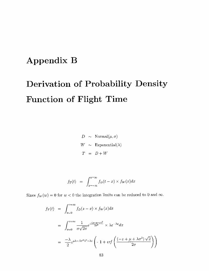
Appendix B
Derivation of Probability Density
Function of Flight Time
D ~ Normal(p,,a)
W ~ Exponential(A)
T = D+W
fT(t)= L0fD(t - x) x fw(x)dx
Since fw(w) = 0 for w < 0 the integration limits can be reduced to 0 and oo.
fDz - x) xfw(x)dx
f O 1 -(z_ -jd)
Sex=0 I x AeAxdxX=0 a -/2-7
-A eA+5o2A2 -Az
2+ erf(Z + y + A2) V2
2a
83
fT(t) =

84

Appendix C
Weather Scenarios
Scenario 1 MFA
Scenario 2 adFRA
Scenario 3 MUC
Scenario 4 MUCh
Scenario 5 MA
FRAScenario 6 MUCFRA
Scenario 7 MUGFRAScenario 8 MUG
FRA
Scenario 9 MUGFRA
Scenario 10 MUG
Scenario 11 FRA
8 12time [UTC
VFRMVFRIFRLowVis
16 20 24
85
0 4
"4, Fl-; ]
4,q x ,,l, MA
'77
MONO W

Scenario 12
Scenario 13
Scenario 14
Scenario 15
Scenario 16
Scenario 17
Scenario 18
Scenario 19
Scenario 20
Scenario 21
Scenario 22
Scenario 23
Scenario 24
Scenario 25
Scenario 26
Scenario 27
Scenario 28
FRMU
FRMU
FRMU
FRMU
FRMU
FRMU
FRMU
FRMU
FRMU
FRMU
FRMU
FRMU
FRMU
FRML
FRML
FRmL
Scenario 29 ML
AC
A
A
AC
AC
AC 41AC "
AC
IAIC
LAIC
LAIC
LA
IC
IAIC
IA
IAIC
IAIC
0 4 8 12 16 20 24time [UTC]
VFRMVFRIFRLowVis
86

Bibliography
[1] Carmen Systems AB. Carmen Integrated Operations Control - Prod-
uct Sheet. http://www.carmen. se/airproducts/pdf/airintegrated_
operationscontrol.pdf, 2004. accessed on Feb. 02, 2006.
[2] J. Abara. Applying Integer Linear Programming to the Fleet Assignment Prob-
lem. Interfaces, 19(4):20-28, 1989.
[3] Deutsche Lufthansa AG. Zahlen, Daten, Fakten 2000/2001. Lufthansa Basis,
60546 Frankfurt am Main, Germany, 2001.
[4] Claudine Biova Agbokou. Robust Airline Schedule Planning: Review and Devel-
opment of Optimization Approaches. Master's thesis, Massachusetts Institute of
Technology, Department of Aeronautics and Astronautics, September 2001.
[5] Yana Ageeva. Approaches to Incorporating Robustness into Airline Scheduling.
Master's thesis, Massachusetts Institute of Technology, Department of Electrical
Engineering and Computer Science, August 2000.
[6] Massachusetts Port Authority. Airport Programs - Environmental - How Logan
Operates. http: //www. massport. com/logan/airpo _no isehowlo .html.
[7] Elisabeth Bly. Effects of Reduced IFR Arrival-Arrival Wake Vortex Separation
Minima and Improved Runway Operations Sequencing on Flight Delay. Master's
thesis, Massachusetts Institute of Technology, Department of Aeronautics and
Astronautics, February 2005.
87

[8] John Van de Vegte. Feedback Control Systems. Prentice Hall, Upper Saddle
River, NY, 07458, USA, third edition, 1993. ISBN 0130163791.
[9] Institut du Transport Aerien. Cost of Air Transport Delay in Europe - Final
Report, November 2000.
[10] Bob Rae et al. Ontario - a Leader in Learning, February 2005. ISBN 077947564X.
[11] Eurocontrol Central Office for Delay Analysis. Enhanced coda. http: //www.
eurocontrol.int/eCoda/.
[12] Steering Committee for the Review of Government Service Provision. Report
on Government Services 2005. Commonwealth of Australia, LB 2 Collins Street
East Post Office, Melbourne VIC 8003, Australia, 2005. ISBN 1740371607.
[13] Waitakere City Council Strategic Group. Key performance indicator council ser-
vices survey. http: //www. waitakere. govt. nz/AbtCnl/kpisurveys. asp. ac-
cessed on Jan. 15, 2006.
[14] John-Paul Clarke, Terran Melconian, Elizabeth Bly, and Fabi Rabbani. MEANS
- MIT Extensible Air Network Simulation. Simulation, 81(12), December 2005.
[15] OAG Worldwide Limited. OAG MAX - System Version 6.1. Data CD-ROM.
[16] Terram Melconian. MEANS User Documentation. Massachusetts Institute of
Technology, 77 Massachusetts Avenue, Cambridge, MA, 02139, USA.
[17] Terran Melconian. Effects of Increased Nonstop Routing on Airline Cost and
Profit. Master's thesis, Massachusetts Institute of Technology, Department of
Aeronautics and Astronautics, September 2001.
[18] Terran Melconian and Elizabeth Bly. MEANS Programming Documentation.
Massachusetts Institute of Technology, 77 Massachusetts Avenue, Cambridge,
MA, 02139, USA.
88

[19] United Parcel Service of America Inc. Operating in Unison - 2004 UPS Corporate
Sustainability Report. 55 Glenlake Parkway, Atlanta, GA, 30328, USA, June
2005.
[20] The Court of Justice of the European Communities. Judgment of the Court
(Grand Chamber) in case c-344/04, the Queen on the application of Interna-
tional Air Transport Association, European Low Fares Airline Association v
Department for Transport, January 2006.
[21] Curtin University of Technology. Annual Report 2004. GPO Box U1987 Perth,
WA, 6845, Australia, 2005.
[22] Bureau of Transportation Statistics. Airline On-Time Statistics and De-
lay Causes. http: //www.transtats. bts.gov/OTDelay/ot-delaycausel. asp,
October 2005.
[23] Katsuhiko Ogata. Modern Control Engineering. Prentice-Hall International, Inc,
second edition, 1990. ISBN 0135987318.
[24] The European Parliament and the Council of the European Union. Regulation
(EC) No 261/2004 of the European Parliament and of the Council of 11 February
2004 establishing common rules on compensation and assistance to passengers
in the event of denied boarding and of cancellation or long delay of flights, and
repealing Regulation (EEC) no 295/91 - commission statement, February 2004.
[25] Eric T. Peterson. Web Site Measurement Hacks. OReilly, 1005 Gravenstein
Highway North, Sebastopol, CA, USA, 1 edition, 2005. ISBN 0596009887.
[26] Oxford University Press. Oxford English Dictionary. Oxford University Press,
Oxford, United Kingdom, draft revision edition, December 2001.
[27] National Weather Service. ADDS - METARs Help Page. http: //adds.
aviationweather.noaa.gov/metars/description-ifr.php. accessed on Feb.
05, 2006.
89

[28] Georgetown University University Information Services. Data warehouse: Glos-
sary. http://uis.georgetown.edu/departments/eets/dw/GLOSSARY0816.
html. accessed on Feb. 05, 2006.
[29] Barry Craig Smith. Robust Airline Fleet Assignment. PhD thesis, Georgia
Institute of Technology, Industrial and Systems Engineering, August 2004.
[30] Ashish Tewari. Modern Control Design. John Wiley & Sons Ltd, Baffins Lane,
Chichester, West Sussex, P019 1UD, United Kingdom, 2002. ISBN 0471496790.
[31] DFS Deutsche Flugsicherung GmbH Geschftbereich Tower (TWR/FP). Studie
zur Kapazitdt an den Flughdfen mit DFS-Flugplatzkontrolle. Am DFS-Campus
10, 63225 Langen, Germany, 2003.
[32] Edith Cowan University. Annaual Report 2004. Joondalup Drive, Joondalup,
WA, 6027, Australia, 2005.
90


![Operational Impact of the Baseline Integrated Arrival ... · Transportation System (NextGen) program [1], airline operators and the broader aviation community. The field demonstration](https://img.pdfslide.us/doc/110x75/5f482cc1af8cbb49fa0b480a/operational-impact-of-the-baseline-integrated-arrival-transportation-system.jpg)