Embed Size (px)
Citation preview

Dissertations and Theses
12-2015
An Approach to Automotive Electrification and Testing An Approach to Automotive Electrification and Testing
Christopher Rowe
Follow this and additional works at: https://commons.erau.edu/edt
Part of the Electrical and Computer Engineering Commons
Scholarly Commons Citation Scholarly Commons Citation Rowe, Christopher, "An Approach to Automotive Electrification and Testing" (2015). Dissertations and Theses. 239. https://commons.erau.edu/edt/239
This Thesis - Open Access is brought to you for free and open access by Scholarly Commons. It has been accepted for inclusion in Dissertations and Theses by an authorized administrator of Scholarly Commons. For more information, please contact [email protected].

AN APPROACH TO AUTOMOTIVE ELECTRIFICATION AND TESTING
By
Christopher Rowe
A Thesis Submitted to the College of Engineering Department of Electrical Engineering
in Partial Fulfillment of the Requirements for the Degree of Master of Science in
Electrical Engineering
Embry-Riddle Aeronautical University
Daytona Beach, Florida
December 2015

AN APPROACH TO AUTOMOTIVE ELECTRIFICATION AND TESTING
By
Christopher Rowe
This thesis was prepared under the direction of the candidate’s Thesis Committee Chair, Dr. Ilteris Demirkiran, Department of Electrical and Computer Engineering, and has been approved by the thesis committee. It was submitted to the Department of Electrical and
Computer Engineering and was accepted in partial fulfillment of the requirements for the degree of Master of Electrical and Computer Engineering.
Thesis Review Committee:
____________________________ Ilteris Demirkiran, Ph.D.
Committee Chair
____________________________ Thomas Yang, Ph.D. Committee Member
____________________________ Patrick N. Currier, Ph.D.
Committee Member
____________________________ Maj Mirmirani, Ph.D.
Dean, College of Engineering
____________________________ Christopher Grant, Ph.D.
Associate Vice President of Academics
____________________________ Jianhua Liu, Ph.D.
Master's Program Coordinator, Electrical and Computer Engineering
__________ Date

iii

1. Acknowledgements
This thesis would not have been possible without the guidance and inspiration
received from my thesis advisor, Dr. Ilteris Demirkiran, Dr. Thomas Yang, and also my
EcoCAR advisor, Dr. Patrick Currier.
I would like to acknowledge my teammates on the Embry-Riddle EcoCAR 2-3
team that have spent countless hours working to build the 2013 Malibu
I would also like to thank the EcoCAR 2-3 competition, General Motors, and
Argonne National Laboratory for providing the basis and inspiration for this research.
iv
2. Abstract
Researcher: Christopher Rowe
Title: An Approach to Automotive Electrification and testing
Institution: Embry-Riddle Aeronautical University
Degree: Master of Science in Electrical and Computer Engineering
Year: 2015
In order to compete in the EcoCAR 2 competition, Embry-Riddle Aeronautical
University has redesigned the Powertrain of a 2013 Chevrolet Malibu into a plug-in hybrid
electric vehicle. This endeavor was made possible by the EcoCAR 2 competition sponsored
by the Department of Energy, General Motors, and Argonne National Laboratory. The
Powertrain was changed from a conventional internal combustion engine with start/stop
capability, to a fully electric Powertrain, with a diesel generator, and plug in charging
capability. This paper will cover the electrical work performed on the vehicle during the
summer prior to year three of the competition, EcoCAR 2 year three, and preliminary work
for EcoCAR 3 year one competition. The main focus of this paper will be on the electrical
system integration and vehicle testing. Some of the systems include for EcoCAR 2 are the
Selective Catalytic Reduction system, high voltage cabling optimization, CAN bus
network, and charging system. For EcoCAR 3, the design and build of a high voltage
distribution box, for bench testing, will be discussed. Simulations of the high voltage bus
are also explored to gain insight into the voltage ripple and resonant frequency of the high
voltage system in the vehicle.
v

3. Table of Contents 1. Acknowledgements ...................................................................................... iv
2. Abstract ......................................................................................................... v
3. Table of Contents ......................................................................................... vi 4. Table of Figures ......................................................................................... viii 5. Introduction ................................................................................................. 12
5.1 EcoCAR 2: Embry-Riddle Vehicle Architecture [2] .............................. 13
5.1.1 Battery Pack .......................................................................................14
5.1.2 Powertrain Components .....................................................................15
5.1.3 Power Generation Components ..........................................................15
5.1.4 Plugin Charging Components ............................................................15
5.1.5 Regenerative braking ..........................................................................16
5.1.6 Diesel generator Power Plant .............................................................17
5.2 List of Acronyms ..................................................................................... 18
5.3 Thesis Statement ..................................................................................... 20
6. Literature Review........................................................................................ 21
7. Methodology ............................................................................................... 26
7.1 Vehicle Wiring ........................................................................................ 26
7.1.1 Soldering Vs. Crimping and Wire Preparation ..................................26
7.1.2 Wire Sizing .........................................................................................34
7.1.3 Fusing .................................................................................................36
7.2 SCR ......................................................................................................... 40
7.3 Can Bus ................................................................................................... 43
7.4 HV Charging ........................................................................................... 44
7.5 GM vs. ERAU Drive Testing Procedure ................................................. 48
7.6 HV Distribution Box ............................................................................... 50
7.6.1 Demo Box Constraints .......................................................................50
7.6.2 Demo Box Basic Design ....................................................................51
7.6.3 Block Diagram ...................................................................................52
7.6.4 Schematic ...........................................................................................53
7.6.5 HV Fusing ..........................................................................................54
7.6.6 HV Test Connector Fusing .................................................................55
7.6.7 Torque Specifications .........................................................................55
7.7 HV Simulation......................................................................................... 56
vi

8. Results ......................................................................................................... 62
8.1 Vehicle Wiring ........................................................................................ 62
8.1.1 Low Voltage .......................................................................................62
8.1.2 High Voltage ......................................................................................66
8.2 SCR ......................................................................................................... 72
8.3 Can Bus ................................................................................................... 74
8.4 HV charging system design..................................................................... 76
8.5 Vehicle Testing ....................................................................................... 82
8.5.1 GM vs. ERAU Drive Test Results .....................................................82
8.5.2 Zero to Sixty .......................................................................................84
8.5.3 Regenerative Braking .........................................................................85
8.5.4 Side Skirts Aero Test ..........................................................................87
8.6 HV Distribution Box Design ................................................................... 89
8.7 HV Simulation......................................................................................... 94
9. Conclusion .................................................................................................. 99
10. Future work ............................................................................................... 100
11. Bibliography ............................................................................................. 102
vii

4. Table of Figures Figure 1: Series PHEV General Architecture ....................................................... 12 Figure 2: ERAU Series Architecture .................................................................... 13 Figure 3: ESS Battery Pack................................................................................... 14 Figure 4: BRUSA HV Charger ............................................................................. 16 Figure 5: Diesel Generator in Engine Bay ............................................................ 17 Figure 6: Frequencies Identified ........................................................................... 24 Figure 7: frequency Range to Avoid ..................................................................... 24 Figure 8: Voltage Ripple Experiment Results ...................................................... 25 Figure 9: Pre-Tinned Conductors .......................................................................... 27 Figure 10: Soldered Conductors ........................................................................... 27 Figure 11: Heat Shirked Connection..................................................................... 27 Figure 12: Pre-Tinned Conductors ........................................................................ 28 Figure 13: Lashing of Pre-Tinned Conductors ..................................................... 28 Figure 14: Soldered Connection ........................................................................... 28 Figure 15: Heat Shirked Connection..................................................................... 28 Figure 16: Initial Wrap for Western Union........................................................... 29 Figure 17: Completed Wrap for Western Union................................................... 29 Figure 18: Soldered Western Union ..................................................................... 29 Figure 19: Typical Crimping Tools ...................................................................... 30 Figure 20: Butt Splice Prior to Wire Insertion ...................................................... 31 Figure 21: Butt Splice Prior to Crimp ................................................................... 31 Figure 22: Properly Crimped Butt Splice ............................................................. 31 Figure 23: Butt Splice with Heat Shrink ............................................................... 31 Figure 24: Wire with Weather Seal ...................................................................... 32 Figure 25: Wire with no Weather Seal ................................................................. 32 Figure 26: Typical Crimps Terminal Pins ............................................................ 32 Figure 27: Sealed Terminal ................................................................................... 32 Figure 28: Unsealed Terminal .............................................................................. 33 Figure 29: Crimped Terminals .............................................................................. 33 Figure 30: Wire Strippers...................................................................................... 33 Figure 31: Proper Wire ......................................................................................... 34 Figure 32: Extra Insulation ................................................................................... 34 Figure 33: Nicked Insulation ................................................................................ 34 Figure 34: Over twist ............................................................................................ 34 Figure 35: Bent Conductors .................................................................................. 34 Figure 36: Nicked / Cut Conductors ..................................................................... 34 Figure 37: Crushed Conductor .............................................................................. 34 Figure 38: Common Automotive Fuses ................................................................ 38 Figure 39: Fuse Time-Current Characteristic Curves ........................................... 40 Figure 40: SCR Schematic .................................................................................... 42 Figure 41: CAN Bus Signals................................................................................. 43 Figure 42: Basic CAN Bus Diagram .................................................................... 44 Figure 43: J1772 Schematic [10] .......................................................................... 46 Figure 44: Charging Schematic ............................................................................ 47 Figure 45: Aerodynamic Modifications ................................................................ 50
viii

Figure 46: 2D CAD Drawing ................................................................................ 51 Figure 47: HV Demo Box Block Diagram ........................................................... 52 Figure 48: HV Fuse Curve .................................................................................... 55 Figure 49: HV Simulation Simulink Model.......................................................... 57 Figure 50: Model Measurements .......................................................................... 57 Figure 51: ESS Battery Subsystem ....................................................................... 59 Figure 52: HVAC Subsystem ............................................................................... 59 Figure 53: BRUSA Subsystem ............................................................................. 60 Figure 54: Inverter Subsystem .............................................................................. 61 Figure 55: DC/DC Subsystem .............................................................................. 61 Figure 56: Bad Crimp w/ Insulation Crushed ....................................................... 63 Figure 57: Bent Crimp .......................................................................................... 63 Figure 58: Lack of Conductor in Crimp ............................................................... 63 Figure 59: Inverter Configuration 0 Wiring.......................................................... 65 Figure 60: Inverter Configuration 1 Wiring.......................................................... 65 Figure 61: New 12V Distribution ......................................................................... 65 Figure 62: Inside 12V Distribution Box ............................................................... 66 Figure 63: HV Block Diagram .............................................................................. 67 Figure 64: HV Before Length Reduction.............................................................. 68 Figure 65: HV After Length Reduction ................................................................ 68 Figure 66: Inside Front DDE ................................................................................ 68 Figure 67: HV Cable Sleeving Test ...................................................................... 69 Figure 68: HV Cable, Med. Force, 10 reps ........................................................... 69 Figure 69: Sleeving, Med. Force, 10 reps ............................................................. 70 Figure 70: Sleeving, Heavy Force, Until Failure .................................................. 70 Figure 71: Traction Motor with Gland Plate Removed ........................................ 71 Figure 72: NH3 Sensor .......................................................................................... 72 Figure 73: SCR Tank and Body to SCR Harness Connector ............................... 72 Figure 74: NH3 Injector ........................................................................................ 73 Figure 75: SCR Power Distribution Box .............................................................. 73 Figure 76: Old ERAU CAN .................................................................................. 75 Figure 77: New ERAU CAN ................................................................................ 75 Figure 78: Vehicle signal Diagram ....................................................................... 76 Figure 79: Charging Simulation............................................................................ 77 Figure 80: Vehicle Proximity and Control Pilot Controller.................................. 78 Figure 81: Control Pilot Normal Operation .......................................................... 80 Figure 82: Control Pilot Fault ............................................................................... 81 Figure 83: Level 1 120V Charge .......................................................................... 81 Figure 84: Level 2 220V Charge .......................................................................... 81 Figure 85: GM Test Data ...................................................................................... 83 Figure 86: ERAU Test Data .................................................................................. 83 Figure 87: Vehicle 0 to 60 mph data ..................................................................... 85 Figure 88: Regenerative Braking Data ................................................................. 86 Figure 89: Aero Test No Side Skirts ..................................................................... 88 Figure 90: Aero Test with Side Skirts................................................................... 88 Figure 91: HV Cable step 1 .................................................................................. 90
ix

Figure 92: HV Cable step 2 .................................................................................. 90 Figure 93: HV Cable step 3 .................................................................................. 90 Figure 94: HV Cable step 4 .................................................................................. 90 Figure 95: HV Cable step 5 .................................................................................. 90 Figure 96: HV Cable step 6 .................................................................................. 90 Figure 97: HV Cable step 7 .................................................................................. 90 Figure 98: Cable Ends ........................................................................................... 90 Figure 99: HV Hardware ...................................................................................... 91 Figure 100: Plexiglas ............................................................................................ 91 Figure 101: Separators .......................................................................................... 91 Figure 102: Copper Shielding ............................................................................... 91 Figure 103: GND Plate ......................................................................................... 91 Figure 104: Enclosure ........................................................................................... 91 Figure 105: Gland Apart ....................................................................................... 91 Figure 106: Gland Together .................................................................................. 91 Figure 107: Shielding in Box ................................................................................ 92 Figure 108: Plate with Hardware .......................................................................... 92 Figure 109: Glands Installed ................................................................................. 92 Figure 110: Cables Installed ................................................................................. 92 Figure 111: Test Conn. & HVIL ........................................................................... 92 Figure 112: Box Insulated ..................................................................................... 92 Figure 113: Box Labels 1 ...................................................................................... 92 Figure 114: Box Labels 2 ...................................................................................... 92 Figure 115: Box Labels 3 ...................................................................................... 92 Figure 116: HV test Connector and HVIL Micro Switch ..................................... 93 Figure 117: HV Box Complete ............................................................................. 93 Figure 118: Power Spectral Density 12 kHz......................................................... 95 Figure 119: DC Bus Voltage 12 kHz .................................................................... 96 Figure 120: Spectrum Analyzer 12 kHz ............................................................... 96 Figure 121: Power Spectral Density 911 Hz......................................................... 97 Figure 122: DC Bus Voltage 911 Hz .................................................................... 98 Figure 123: spectrum Analyzer for 911 Hz .......................................................... 98
x

Table of Tables Table 1: AWG Wire Table .................................................................................... 36 Table 2: ATM Cooper Bussmann Automotive Fuses ........................................... 39 Table 3: BRUSA Charging Characteristics .......................................................... 45 Table 4: HV demo box constraints ....................................................................... 50 Table 5: Bolt Torque Specs................................................................................... 56 Table 6: ESS Battery Characteristics .................................................................... 58 Table 7: Control Pilot and Proximity States [10].................................................. 77 Table 8: Vehicle Test Data ................................................................................... 82 Table 9: Simulation Calculated Characteristics .................................................... 94
xi

5. Introduction
EcoCAR 2 is a three year competition sponsored by the Department of Energy,
General Motors, and Argonne National Laboratory. The competition encompasses fifteen
Universities across North America [1]. A 2013 Chevrolet Malibu is donated to each team
where it is converted to an electric hybrid vehicle. EcoCAR 2 challenges students to reduce
the Chevrolet Malibu’s emissions, increase fuel economy, and maintain consumer
acceptability [1]. The mission of EcoCAR 2 is to educate the next generation of automotive
engineers through an unparalleled hands-on, real-world engineering experience. [2]
In this competition, Embry-Riddle Aeronautical University chose to design and
build a plug-in hybrid electrical vehicle (PHEV) using a series architecture. Figure 1 shows
the general series architecture of an electric PHEV. The traction motor, generator, and
internal combustion engine are in the engine bay of the vehicle. The ESS is in the trunk.
The black arrows represent the flow of mechanical energy, and the yellow arrows represent
electrical energy. [2]
Figure 1: Series PHEV General Architecture
12

Series plug-in hybrid vehicles consist of one or more electric motors driving the
wheels, and these motors are powered by a battery. An engine-generator is decoupled from
the wheels at all times and provides supplemental electrical power to drive the vehicle
when needed while charging the battery pack at the same time.
5.1 EcoCAR 2: Embry-Riddle Vehicle Architecture [2]
The placement of major components is represented in Figure 2. The front of the
vehicle is located where the traction motor is located.
Figure 2: ERAU Series Architecture
13

5.1.1 Battery Pack
The Energy Storage Unit (ESS), seen in Figure 3, is composed of six 15S3P
LiFePO4 battery modules from A123. All the modules are in series to get a nominal pack
voltage of 292V.
In order to monitor the modules, a battery management system (BMS) is used
within the ESS. The BMS collects data from each module to track each cell’s voltage level
and temperature. The BMS also monitors the ESS voltage and current levels. The BMS is
necessary in order to ensure the modules are being charged and discharged correctly to
mitigate the chance of causing damage to the modules within the ESS. If a problem is
identified, the BMS will open the contactors connected to the battery modules in order to
disconnect the ESS from the rest of the vehicle's high voltage (HV) systems.
Figure 3: ESS Battery Pack
14
5.1.2 Powertrain Components
The main powertrain components consist of an AM Racing Remy HVH 250-090P
Traction Motor which is coupled to a GKN E-Transmission. As a Series Plug-In Hybrid,
the tractive force supplied to the wheels of the vehicle solely comes from the electric
traction motor.
5.1.3 Power Generation Components
The full electric range of the vehicle is 30 to 40 miles, depending on traffic and
driver habits. To improve consumer acceptability a 1.7 liter GM Diesel Engine coupled to
an AM Racing Remy HVH 250-090S Generator was installed in the vehicle. This genset
acts as a range extender by supplying electrical power to the traction motor and ESS. This
allows the vehicle to keep driving after the ESS has been depleted. The diesel engine does
not provide any torque to the tires of the vehicle.
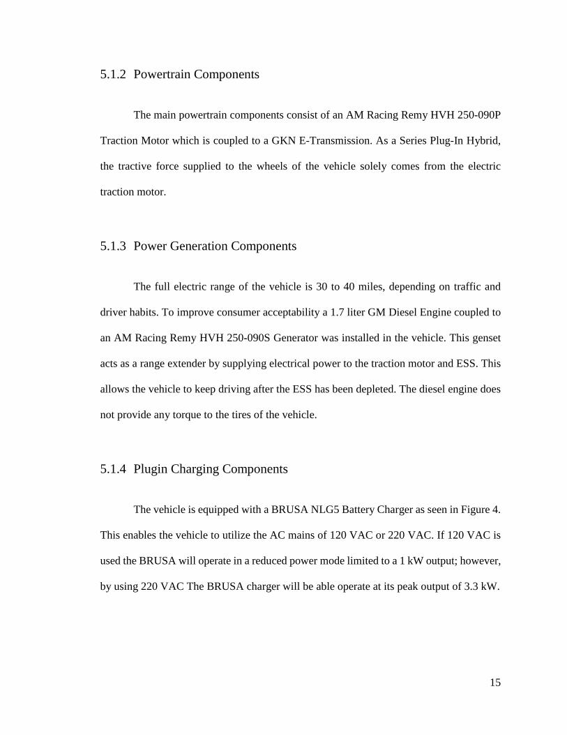
5.1.4 Plugin Charging Components
The vehicle is equipped with a BRUSA NLG5 Battery Charger as seen in Figure 4.
This enables the vehicle to utilize the AC mains of 120 VAC or 220 VAC. If 120 VAC is
used the BRUSA will operate in a reduced power mode limited to a 1 kW output; however,
by using 220 VAC The BRUSA charger will be able operate at its peak output of 3.3 kW.
15

Figure 4: BRUSA HV Charger
The BRUSA inverts the AC power into DC to charge the battery. In order to charge
the LiFePO4 cells in the pack properly, the BRUSA communicates with the battery
management system, located in the ESS, with CAN bus messages to control the charging
process.
5.1.5 Regenerative braking
By using an AC Interior Permanent Magnet (IPM) electric motor (AMR-250P),
regenerative braking can be used for two purposes. The primary purpose is to generate
power back to the battery pack while slowing the vehicle. By recovering this power while
braking, the vehicle is able to extend the time and mileage while the vehicle is operating in
EV mode only. This is important since the longer the vehicle stays in the charge deplete
mode (CD) the longer the diesel engine will stay off. This will reduce the overall vehicle
emissions greatly.
16

The second purpose of regenerative braking is to enhance the EV driving
experience. By using a zero floating point controls strategy, it is possible to drive the
vehicle using mostly the acceleration pedal. It is only necessary to use the brake pedal when
the vehicle is below ~10 MPH or greater braking is required, but for normal city or highway
driving the regenerative braking provides enough braking power to comfortably drive the
vehicle with only the acceleration pedal.
5.1.6 Diesel generator Power Plant
Once the ESS has been depleted to a depth of discharge (DOD) of 20% the vehicle
will enter a charge sustain mode (CS). CS will enable the vehicle to continue driving while
the ESS is in need of charging. In conventional EVs the vehicle must stop driving and plug-
in to charge the ESS, and once the ESS has been re-charged the vehicle can continue
driving. Under CS mode the vehicle will allow the ESS to deplete to 20% and then turn on
a diesel electric generator, seen in Figure 5, to provide power to the ESS and traction motor.
Figure 5: Diesel Generator in Engine Bay
17

5.2 List of Acronyms AC Alternating Current
APM Auxiliary Power Module
AWG American Wire Guage
BCM Body Control Module
BMS Battery Management System
CAN
Controller Area Network
CAT CATalytic converter
CD Charge Depletion
CP Control Pilot
CS Charge Sustaining
DC Direct Current
DDE Distribution and Disconnect Enclosure
DPF Diesel Particulate Filter
E&EC Emissions and Energy Consumption
EMS Energy Management Strategy
ERAU Embry-Riddle Aeronautical University
ESS Energy Storage System (high voltage battery pack)
EV Electric Vehicle
EVSE Electric Vehicle Supply Equipment
GM General Motors
GND Ground
HIL Hardware In the Loop
18

HV High Voltage
HVAC High Voltage Air Conditioning
HVIL High Voltage Interlock Loop
ICE Internal Combustion Engine
LV Low Voltage
MABX Microautobox
MPG Miles Per Gallon
MY Model Year
NOx Nitrogen Oxide
PHEV Plug-in Hybrid Electric Vehicle
PROX Proximity
PSD Power Spectrum Density
PWM Pulse Width Modulated (Square wave)
RPM Revolutions Per Minute
SAE Society of Automotive Engineering
SCR Selective Catalytic Reduction
SIL Software In the Loop
SOC State of Charge
VAC Voltage Alternating Current
YR Year
WOT Wide Open Throttle
19

5.3 Thesis Statement
This paper investigates the strong hybridization of a conventional production
vehicle. The creation of a series plug-in hybrid electric vehicle with extended range
capabilities will be investigated pertaining to the vehicle electrical systems. The main focus
will be on HV and LV system modifications performed on a 2013 Malibu. A secondary
focus will be explored to estimate voltage ripple and resonant frequency by using on HV
bus simulations.
20

6. Literature Review
The basis for this literature review is based around the high voltage simulation
designed for this thesis. While researching papers for electric vehicle high voltage bus
characterization, it became evident there has been little work performed on the high voltage
bus, encompassing the entire bus and HV components, of electric vehicles. In dealing with
resonant frequency, the main focus for research leans toward leveraging resonant
frequency for charging electric vehicles [3]. One such paper titled “Current Ripple
Reduction in 4kW LLC Resonant Converter Based Battery Charger for Electric Vehicles”
describes a resonant controller employed to suppress the low-frequency current ripple in
an LLC resonant converter for EV battery chargers [3]. A part of this paper has a study
with a focus on the affect voltage ripple in the DC-link capacitor, or bulk capacitor, has
within the charger. The point this paper makes is that a small change in voltage on the DC-
link capacitor can result in a large change in ripple current; however, the voltage ripple in
the DC-link capacitor is set to 12 V peak to peak and does not change [3]. The paper does
not look at how the charger can induce the voltage ripple in the DC-link capacitor. This
would be a more accurate representation of the cause of voltage ripple on the system. This
paper also is focused on the charging side of the vehicle dealing with the switching
characteristics of the vehicle charger. Although, the HV simulation of this thesis focuses
on the inverter switching characteristics, both charging and inverter switching
characteristic topologies are very similar.
To help aid in designing the HV simulation a book titled “Introduction to Hybrid
Vehicle System Modeling and Control” was very useful. This book focuses on modeling,
21

control, simulation, and performance analysis of specific systems of electric vehicles.
Vehicle architectures are also discussed with detail in component characterization, and a
systematic approach to develop models, controls, and algorithms [4]. “The Electrical
Engineering Handbook” aided in battery characterization and simple models of a battery.
This book also went in depth into the workings of Inverter switching techniques along with
different methods of powering electric motors with inverters [5]. This helped design the
switching characteristics in the HV simulation described in this paper to more closely
model the proper switching of an inverter.
“Co-Simulation and Harmonic Analysis of a Hybrid Vehicle Traction System”
explores a modern hybrid vehicle design where a three phase traction motor, powered by
n inverter, is connected to a high voltage battery. In order to determine the high frequency
system behavior, the current and voltage harmonics of this system are simulated to estimate
the effect from the switching in the inverter [6]. A frequency analysis was performed on
the bus, from the battery to the inverter, by analyzing the DC bus current ripple. A
frequency of 20 kHz was identified to have the largest power [6]. The model used to
characterize the system has a heavy focus on the inverter itself; however, the model does
not consider any other components commonly seen in electric vehicles. The inverter does
have a major influence on the system; however, modern vehicles no longer simply have a
battery and a traction inverter in the HV electrical system.
“Development and Future Issues of High Voltage Systems for FCV” details a
vehicle designed by the Nissan Motor Co., Ltd. The vehicle delivered was the 2005 X-
22

TRAIL FCV, and was available to customers on April 2006 in Japan [7]. This paper details
the vehicles architecture as well as the workings of a DC/DC converter used in the vehicle
to boost the vehicle voltage from a fuel cell to power the traction inverter. By using a
DC/DC converter to amplify bus voltage the voltage ripple on the bus is amplified. This is
due to having both the DC/DC converter and traction inverter on the same bus while
switching at the same time. This paper does not go into detail of what problems could arise
from multiple high power switching devices operating at the same time [7]. This is a similar
issue in the HV simulation designed for this thesis. There can be two inverters providing
power to motors in the simulation designed.
“Design Considerations for High-Voltage DC Bus Architecture and Wire
Mechanization for Hybrid and Electric Vehicle Applications” notes that modern hybrid
electric vehicle no longer have simple HV DC bus designs. Current vehicles have multiple
power converters units and energy storage systems on a single bus [8]. The author also
correctly identifies the fact that each component should meet a set of common HV bus
design requirements besides their own functional requirements. Because of this fact the
author is looking at the system as a whole instead of single components. This paper
describes HV DC bus architecture and component selection particularly for Extended-
Range Electric Vehicle application [8]. Multiple architecture layouts are looked at in this
paper; however, the main focus is on voltage ripple, resonance and voltage transients
during various vehicle drive profiles. The author is able to identify a frequency range that
should be avoided during vehicle operation seen in Figure 6 and Figure 7 [8].
23

Figure 6: Frequencies Identified
Figure 7: frequency Range to Avoid
The author identifies the traction inverter as being the biggest power converter in
the HV bus system. Due to this, the author analyzes target vehicle drive conditions and
identifies critical usage profiles for the inverters. These critical profiles represent worst
case HV bus ripple generated by the inverter [8]. This is used as the basis for the voltage
ripple study. The simulated data from this paper focuses more on voltage transients the
24

actual voltage ripple; however actual experimental data is gathered showing the actual
voltage ripple and is compared to simulation data. The results of this experiment can be
seen in Figure 8 [8].
Figure 8: Voltage Ripple Experiment Results
25

7. Methodology
7.1 Vehicle Wiring
7.1.1 Soldering Vs. Crimping and Wire Preparation
There is an ongoing debate which has been going on for years dealing with circuits
being soldered or crimped. Soldered wires are thought to be brittle and can break overtime;
while, crimped wires are thought to not hold together well over time causing the wire to
release from the crimp. The truth is both soldering and crimping are valid ways to connect
circuits and terminate wires with terminals. For automotive specifically, the OEMs go the
route of crimping almost exclusively. This is due to the vibrations in a vehicle, and the
thought is crimps hold up better to the vibrations. NASA on the other hand uses soldering
on the space shuttle, and it experiences heavy vibrations when launching into space. The
important fact is that each method is performed correctly to prevent potential failures.
7.1.1.1 Soldering
There are several methods for soldering conductors together. The most common
techniques are the lap splice, lash splice, and the western union. With each splice it is
important to use just enough solder to form the connections. Too much solder can wick
into the conductor and go under the insulation. This will cause the wire to become stiff and
could break over time. If not enough solder is used the conductors can pull apart. In most
26

cases too much solder is usually used. The proper amount of solder will allow a solid
connection between conductors; however, the individual strands of the conductors should
still be able to be seen as in Figure 10.
A lap splice solders conductors together with each conductor straight and soldered
length wise. The conductors should be pre-tined before soldering the conductors together.
This will aid in the transfer of heat during the soldering process. Heat shrink should be
used to cover the connection when finished. A quarter inch of insulation should be removed
for this splice. This process is seen in Figure 9, Figure 10, and Figure 11 [9].
Figure 9: Pre-Tinned Conductors
Figure 10: Soldered Conductors
Figure 11: Heat Shirked Connection
The lash splice is similar to the lap splice. It adds a single strand of wire to “lash”
the pre-tinned conductors together. The extra strand is used to wrap around the conductors
to aid in the soldering process by holding the wires together. This is especially beneficial
27

when a person is soldering by themselves, and cannot hold the wires and soldering iron at
the same time. Heat shrink should be used to cover the connection when finished. A quarter
inch of insulation should be removed for this splice and the single strand should be half an
inch long. This process is seen in Figure 12 through Figure 15 [9].
Figure 12: Pre-Tinned Conductors
Figure 13: Lashing of Pre-Tinned
Conductors
Figure 14: Soldered Connection
Figure 15: Heat Shirked Connection
The western union splice is the most common splice used. The wires can be pre-
tinned prior to solder, but very little solder can be used to aid in wrapping the wires
together. The conductors are wrapped together with at least three turns around each
conductor. This makes sure the conductors will not come apart during the soldering
process. Like the previous splices, just enough solder should be used to connect the
conductors together. The conductor strands will still be visible through the solder. A half
inch of insulation should be removed from each conductor for this splice. This process is
seen in Figure 16 through Figure 18 [9].
28

Figure 16: Initial Wrap for
Western Union
Figure 17: Completed Wrap for Western Union
Figure 18: Soldered Western Union
7.1.1.2 Crimping
Crimping is another viable method for connecting circuits together. Crimping uses
mechanical force to form connections. The amount of force applied to the crimp must be
just right. Too much force and the conductors can be crushed, and too little force will likely
result in the conductor falling out of the crimp. Special tooling is required for each different
crimp to ensure the crimp will not fail prematurely. Figure 19 shows the tooling typically
used for crimping. Each kind of crimp has a matching tool to perform the job. The better
tools use a ratcheting feature which will not release the tool until the proper force has been
applied to the crimp. Once the right amount of force is applied the ratcheting feature will
allow the tool to release.
29

Figure 19: Typical Crimping Tools
Crimping is performed for two main reasons. The first is to connect separate
conductors together, and the second reason is to crimp a terminal pin to the end of a wire
for insertion into a connector. For vehicles, crimping is mostly done to connect terminal
pins to the ends of wires. Just like soldering, the insulation of the wire must be stripped off
the conductor before crimping, and the amount of insulation removed depends on the type
of crimp being performed. The amount of insulation removed is usually a quarter of an
inch.
Butt splices are used to crimp multiple conductors together. The number of
conductors can be easily adjusted using this crimping method. Two wires are usually
connected; however, multiple wires can be inserted into a single end of the butt splice. To
do this, the total number of wires cross-sectional areas must add up to what the butt splice
is rated for. If the added cross-sectional area is greater than what the butt splice is rated for
then the wires will either not fit, or the conductors will be crushed when crimped. If the
added cross-sectional area is less than what the butt splice is rated for then the wires will
fall out of the butt splice. To properly prepare a wire for a butt splice, the wire should be
inserted into the butt splice for an initial measurement for trimming the insulation. The
insulation should not enter the butt splice, and about a millimeter of the conductor should
30

be seen between the insulation and butt splice. There is also a hole in the middle of the butt
splice. This is used to ensure the conductor is inserted fully into the butt splice. The butt
splice process is seen in Figure 20 through Figure 23 [9].
Figure 20: Butt Splice Prior to Wire
Insertion
Figure 21: Butt Splice Prior to Crimp
Figure 22: Properly Crimped Butt Splice
Figure 23: Butt Splice with Heat Shrink
Terminal pins can be either weather sealed, or not weather sealed. Wires with and
without a wire seal can be seen in Figure 24 and Figure 25. Terminals being installed in a
connector that could come in contact with fluids, connectors in an engine bay, need to be
weather sealed. If the terminal will be inside the vehicle and protected from the elements
the terminal will not need to be weather sealed.
31

Figure 24: Wire with Weather Seal
Figure 25: Wire with no Weather Seal
The sealed and unsealed terminals are effectively the same; however, the two tangs, or
wings, that grip the insulation of the wire are typically bigger for the sealed terminals. This
allows the seal to also be griped by the tangs. See Figure 27. Just as the butt splice, the
manufacturer documentation should be referenced for proper preparation of the wire.
Typically a quarter inch of insulation is removed from the conductor. The wire can then be
place into the terminal pin to test the fit of the wire. The conductor should pass the core
tangs, or wings, by about a millimeter. If there is a little extra length that is fine. The
insulation should be the only thing crimped by the insulation tangs. If the conductor is
being grabbed the insulation could pull away from the conductor. Once the wire is ready,
the terminal pin and wire is crimped together using a proper crimper for the terminal pin.
The process for crimping a terminal pin is seen in Figure 26 through Figure 29 [10].
Figure 26: Typical Crimps Terminal Pins
Figure 27: Sealed Terminal
32

Figure 28: Unsealed Terminal
Figure 29: Crimped Terminals
7.1.1.3 Wire Preparation
Proper wire stripping tools should be used to remove wire insulation from a
conductor. Wire strippers, Figure 30, are machined in such a way that they will not damage
either the wire insulation or conductor while using the tool.
Figure 30: Wire Strippers
After stripping the wire, the remaining insulation should not exhibit any damage
such as nicks, cuts, crushing, or charring. [9] Conductors shall also not exhibit any damage.
The conductor should not be scraped, bent, nicked, crushed, or cut [9]. Any damage to the
conductor will lower the ampacity of the wire, and cause a point of failure. If either the
33

insulation or conductor is damaged during preparation the end should be cut off and
remade. Figure 31 shows a properly made wire end, and Figure 32 through Figure 37 shows
ends needing to be remade [11].
Figure 31: Proper Wire
Figure 32: Extra Insulation
Figure 33: Nicked
Insulation
Figure 34: Over twist
Figure 35: Bent
Conductors
Figure 36: Nicked / Cut
Conductors
Figure 37: Crushed Conductor
7.1.2 Wire Sizing
“Selecting the correct wire gauge ensures the proper voltage supply to an electrical
device and prevents the cable from overheating” [10]. A wire can be thought of a long
resistor; therefore, resistance and ampacity should be considered when selecting the proper
wire gauge. “All electrical conductors have some resistance to the flow of electrical current.
34

The resistance of a cable increases as the cross sectional area or gauge decreases.
Conversely, cables with a larger cross section have less resistance and thus, a higher
ampacity. The current in a cable can cause the cable to heat up due to the conductor’s
(copper) resistance. When current increases to a level high enough to raise the internal
conductor temperature to a point that exceeds the maximum temperature rating of the cable,
the insulation begins to degrade” [10].
If the insulation degrades to the point of failing the insulation will begin to melt.
This will likely result in a short occurring in the circuit causing component malfunction.
Also, as current increases in a wire the voltage drop will also increase across the wire.
Voltage drop reduces the overall voltage delivered from a supply. Common practices is to
have no more than a 2% voltage drop from the power source to a device. For a 14V system,
like on a conventional vehicle, the voltage should not fall below 13.72V. For example, a
water pump draws 4 amps of current, the total wire length, positive and negative side, is
10 feet, and the wire is an 18 AWG wire. Voltage drop calculation steps given below using
Table 1.
• Voltage drop using Ohm’s Law: Vdrop = I*R • Resistance for 10 ft of 18 AWG wire : R = 0.006385*10 = .06385 Ω • Current draw of pump: I = 4 A • Voltage drop from wire: Vdrop = 4*.06385 = .2554 V • Actual voltage supplied to pump: Vpump = 14-.2554 = 13.74 V • % voltage drop: %𝑉𝑉𝑑𝑑𝑑𝑑𝑑𝑑𝑑𝑑
14−13.7414
∗ 100 = 1.86 %
A voltage drop of 1.86 % is the end result by using a 10 ft 18 AWG cable to supply
the pump with 4 A of current. According to Table 1, an 18 AWG wire can continuously
supply 16 A; however, in order to supply the correct voltage to the pump the 18 AWG is
35

needed. A 22 AWG wire is also able to carry a 4 A draw, but due to the length of the wire
the voltage drop will greatly increase. See below calculation.
• Voltage drop using Ohm’s Law: Vdrop = I*R • Resistance for 10 ft of 22 AWG wire : R = 0.01614*10 = .16 Ω • Current draw of pump: I = 4 A • Voltage drop from wire: Vdrop = 4*.16 = .64 V • Actual voltage supplied to pump: Vpump = 14-.64 = 13.36 V • % voltage drop: %𝑉𝑉𝑑𝑑𝑑𝑑𝑑𝑑𝑑𝑑
14−13.3614
∗ 100 = 4.57 %
If a 22 AWG is used to power the pump the voltage drop of 4.57 % exceeds the 2
% maximum voltage drop.
Table 1: AWG Wire Table
AWG gauge Conductor Diameter Inches Ohms per 1000 ft. Maximum amps
0000 0.46 0.049 380 000 0.4096 0.0618 328 00 0.3648 0.0779 283 0 0.3249 0.0983 245 2 0.2576 0.1563 181 4 0.2043 0.2485 135 6 0.162 0.3951 101 8 0.1285 0.6282 73 10 0.1019 0.9989 55 12 0.0808 1.588 41 14 0.0641 2.525 32 16 0.0508 4.016 22 18 0.0403 6.385 16 20 0.032 10.15 11 22 0.0254 16.14 7
7.1.3 Fusing
36

“The fuse is a simple and reliable safety device. It is second to none in its ease of
application and its ability to protect people and equipment. The fuse is a current-sensitive
device. It has a conductor with a reduced cross section (element) normally surrounded by
an arc-quenching and heat-conducting material (filler). The entire unit is enclosed in a body
fitted with end contacts” [5].
Once the correct wire size has been determined for a given circuit, the wire now
needs to be protected from damage, insulation failure from high temperature, for both
extended high currents and short circuit current conditions. The proper fusing and wire
sizing is the foundation for a safe electrical system. Fuses must be sized to interrupt the
flow of current before the conductor reaches its ampacity. Improper fuse sizing can result
in dangerous thermal failures in an electrical harness, as wires heat up potentially melting
the insulation.
Fuses have specific voltage ratings that should not be exceeded to ensure proper
safety. When a fuse blows, it must be able to extinguish the electrical arc in the conduction
path in a short amount of time, or current may continue to flow allowing a fault to not be
corrected. To accomplish this, general automotive fuses for use in low voltage systems are
rated to 32 V. Figure 38 shows fuses typically used for automotive applications.
37

Figure 38: Common Automotive Fuses
When determining the correct fuse for an application one must keep in mind the
device being powered is not what the fuse will be protecting. The fuse is protecting the
wires. The wire for a given device should be sized to provide the correct current for the
device, but is also capable of carrying much more current safely. This is due to adjusting
the wire size due to the voltage drop caused by the resistance and length of the wire. What
the fuse is protecting is a worst case scenario of a hard fault, or short, in a wire. This can
be cause by a wire accidentally being cut, chemical damage of the insulation, or the
insulation being worn away by chafing. Whatever the cause of the loss of insulation the
bare wire will eventually come into contact with the frame of the vehicle which shorts the
wire to ground. At this point the wire has very little resistance and will pull an amount of
current greater than the wire can handle. Going from the above example of the pump, an
18 AWG wire at 10 feet has 0.16 Ω of resistance. At 14 V, for automotive, and 0.16 Ω the
wire will pull close to 88 amps of current. In this case if the fuse doesn’t blow the insulation
of the wire will completely fail potentially causing damage to the vehicle and/or fire.
Table 2 shows the common amp ratings and color codes for automotive fuses. This
standard is used for all manufactures.
38

Table 2: ATM Cooper Bussmann Automotive Fuses Product Code Amp rating
Body Color Voltage Rating DC
ATM-2 Gray 32V ATM-3 Violet 32V ATM-4 Pink 32V ATM-5 Tan 32V ATM-7 ½ Brown 32V ATM-10 Red 32V ATM-15 Light Blue 32V ATM-20 Yellow 32V ATM-25 White 32V ATM-30 Green 32V
Some components in a vehicle will cause an inrush current when turning on. An
inrush current is a current that lasts for a short period of time, usually less than a second,
just as the device is turning on. It is a much larger current than what is typically drawn
during normal operation; therefore, the inrush current should be taken into consideration
when sizing a fuse. A fuse blows when the element inside the fuse melts. This is caused by
the current heating the element. It is possible to have a fuse carry a current greater than
what the fuse is rated for as long as it is for a short period of time. Figure 39 gives the time-
current characteristic curves for each automotive fuse. This can be used to ensure a fuse
will not blow due to an inrush current.
39

Figure 39: Fuse Time-Current Characteristic Curves
7.2 SCR
As emissions regulation become ever stricter there has become a need to reduce
emissions of today’s vehicles. Diesel engines have an advantage over conventional
gasoline engines since they produce 20% less CO2; however, diesel engines produce more
NOx [12]. By 2025 the US EPA is calling for a 75% reduction in NMOG+NOx, and Europe
40

will also be calling for a heavy reduction of NOx emissions [13]. To help reduce emissions
on the Malibu a Selective Catalytic Reduction (SCR) system is installed on the vehicle’s
exhaust.
The mechanical team handled the physical mounting of the SCR components, while
the electrical team wired everything together. All of the components used in the SCR
system, detailed in Figure 40, were sourced from a Chevrolet Cruze. Pinouts of each
component were available to the team by using parts from a General Motors vehicle, but
datasheets were not supplied. This made it difficult to control both the injector and pump.
Testing needed to be completed to properly control each component. Each component was
for current draw to properly size power wires. The current draw and wire size for each
component is listed in the schematic of Figure 40.
41

Figure 40: SCR Schematic
42

7.3 Can Bus
A modern vehicle is made up of many different controllers to run the vehicle, and
it is often necessary for these controllers to share data with each other. In order to share
information a network is formed with controllers called a CAN bus, or Controller Area
Network Bus, this type of communication uses two separate wires twisted together to send
signals. These wires are called CAN High and CAN Low. Figure 41 shows the signals
when viewed on a scope. CAN_H is from 2.5 V to 3.5 V, and CAN_L is from 2.5 V to 1.5
V [14]. The CAN system takes the difference between the two voltages to transmit data in
binary. In the recessive state of 0 volts the signal represents a binary 1, and in the dominant
state the signal will be 2 volts representing a binary 0. Being a twisted pair with a
differential type signal, the CAN bus is highly immune to noise. The twisted wires provide
noise immunity, but if noise does contaminate the signal it will add contamination to both
CAN_H and CAN_L. Taking the difference of CAN_H and CAN_L will filter out any
noise in the signals due to both signals being affected the same [14].
Figure 41: CAN Bus Signals
43

Figure 42 gives the basic layout of the CAN bus. The bus can have as many nodes,
or controllers, as desired in the system. The two main design considerations must be
followed. First, there must be terminating resistors of 120 ohms at the far ends of the bus.
This matches the impedance across the entire bus to 60 ohms, and ensures the signals on
the bus do not degrade [14]. If the terminating resistors are left out a signal will reflect back
onto the bus after it has been sent and can corrupt the next message. The second design
consideration is to keep the stub lengths from the main bus to each node as short as possible.
As the stub length increases the impedance will also increase. If the stub length becomes
too great then messages on the bus will begin to reflect back onto the buss causing messages
to be lost. Best practice is to keep the stub lengths less than two inches [14].
Figure 42: Basic CAN Bus Diagram
7.4 HV Charging
By using the J1772 standard, the vehicle is able to charge using a variety of common
and accessible electric vehicle supply equipment (EVSE). The two most common ways the
44

ERAU EcoCAR is charged is by using a portable charger, or a level 2 charging station
located on the ERAU campus electric vehicle parking spaces. The portable charger is
limited to a common 120 VAC outlet which allows the BRUSA to charge the battery pack
at a max of 1 kW. The size of the unit allows it to be carried in the vehicle to allow charging
when only a 120 VAC outlet is available. The charging station uses 220 VAC as its voltage
input, and this will enable charging up to 3.3 kW with the BRUSA. Table 3 shows the
charging characteristics of the BRUSA as well as the approximate charging times of the
EVSE used to charge the vehicle.
Table 3: BRUSA Charging Characteristics AC Voltage Charging Equipment Output Power Time to
Charge Pack 120 V Portable 1 kW ~16 hours 220 V Station 3.3 kW ~5 hours
The BRUSA is controlled over CAN by the Battery Management System (BMS)
of the ESS. The BMS sends commands over CAN to the BRUSA for what voltage and
current should be outputted to the ESS. The general high level charging procedure is as
follows:
1. EVSE cordset plugged into vehicle.
2. BRUSA turns on and wakes up the ESS BMS.
3. BMS requests power, and enables the BRUSA to begin charging.
4. BRUSA follows BMS commands to charge the ESS.
To help initiate the charging process, and add levels of safety, the J1772 standard
utilizes Control Pilot (CP) and Proximity circuits. Figure 43 shows the CP and Proximity
45

circuits detailed in the J1772 standard. The Proximity circuit is used to ensure the vehicle
cannot drive while the vehicle is plugged into an EVSE. This is solely for safety. CP has
two functions. The first is also a safety feature where the EVSE is signaled it is safe to
provide power to the vehicle. The second feature of CP is to signal the vehicle what the
max current limit the EVSE is able to supply. This keeps the BRUSA from pulling too
much current from the EVSE. A more detailed explanation of the CP function will be given
in the Results section.
Figure 43: J1772 Schematic [15]
The schematic designed for the charging system is shown in Figure 44 shown
below.
46

Figure 44: Charging Schematic
47

7.5 GM vs. ERAU Drive Testing Procedure
Two separate tests have been performed on the vehicle. The first test was performed
at the General Motors (GM) Milford proving grounds facility. Testing was conducted by
GM-approved test-track drivers, and they followed a drive schedule to mimic a mix of
highway and in-city driving. During the GM testing, the vehicle pulled a small utility trailer
equipped with a SEMTECH DS exhaust emission analyzer. This equipment was used to
gather emissions data from the vehicle throughout the length of the test. Regenerative
braking was not used during the GM testing. Regenerative braking was intended to be used;
however, it was disabled by accident and the test could not be re-run.
The second test was performed by ERAU-approved drivers on the EcoCAR team.
The vehicle was driven on city roads and on the highway to gather the needed data. Due to
instrumentation limitations, emissions data could not be gathered from the vehicle while
testing. Regenerative braking was fully enabled during the ERAU testing. It is important
to note that the GM test was done overnight for 5.5 hours. Due to student schedules, the
ERAU test could only be performed for a little over 2 hours.
For both tests, prior to testing, the vehicle’s ESS is fully charged/balanced and the
fuel tank is filled. The tank is filled by removing the tank from the vehicle enabling the
tank to be weighed. This gives a more precise approximation for fuel consumed while
operating the diesel generator. The vehicle drive cycle is then carried out. Once testing is
completed the vehicle is returned to the garage where the fuel tank is removed from the
48

vehicle for weighing in order to find the total fuel consumed during testing. Lastly, the
vehicles ESS is charged back to 100% SOC.
Simulations have shown that a 10% reduction in drag will result in approximately
a 6% decrease in energy consumption for a majority of drive cycles [16]. The vehicle has
been outfitted with a side-skirting system which will reduce the amount of air spilling out
from the sides of the vehicle underbody. This reduction in spillage will energize the flow
underneath the vehicle and further reduce drag. This will be accomplished with the use of
nylon bristles that act as a weather guard. This will allow a close proximity with the ground
for improved aerodynamics without sacrificing ground clearance. CFD simulations have
shown an approximate 5% reduction in drag. To increase the skirting system’s
effectiveness, the vehicle will also implement aerodynamic wheel covers [17]. These have
shown significant reductions in drag in previous research [18]. These, like the skirting
system, act to reduce the amount of air spilling from the underbody of the vehicle. Since
the vehicle has regenerative braking, reductions in brake cooling are negated. Finally,
vortex generators which act to reduce flow separation on the rear window are installed on
the vehicle [17]. Figure 45 shows the aerodynamic modifications installed on the vehicle
[2].
49

Figure 45: Aerodynamic Modifications
7.6 HV Distribution Box
7.6.1 Demo Box Constraints
To aid the team in component calibration and testing for EcoCAR 3. A HV demo
box has been designed specifically for bench testing of HV components within the lab. The
demo box will also serve as a tool to teach students HV safety and good practices.
Table 4: HV demo box constraints Temperature (due to enclosure) -20 to 80⁰C
Continuous Current 125A
Maximum Operate Voltage 400V
Ingress protection Minimum of IP66/67
Impact resistance IK08/IK09
All materials resistant to automotive fluids Yes
Electrical insulation Totally insulated
Vortex Generators
Side Skirts
50

7.6.2 Demo Box Basic Design
The general HV layout is shown below in Figure 46. The design was kept as simple
as possible to aid in component management; such as, wire bend radius. The 2/0 Cable has
a bend radius of 4.5 in. If a bend was attempted inside of the demo box much of the space
will be wasted. Due to this fact, the HV cables were kept straight to maximize the space in
the box. Another important detail to note is that the extra space was utilized by making it
possible to expand the HV circuitry. This is seen in Figure 46 where there is extra space
for a HV fuse, lugs on the positive buss bar, and space for another lug on the negative buss
bar.
Figure 46: 2D CAD Drawing
51

7.6.3 Block Diagram
Figure 47: HV Demo Box Block Diagram
52

7.6.4 Schematic
53

7.6.5 HV Fusing
The “High Speed Fuse Application guide” document by Cooper Bussmann was
utilized to find the proper fuse rating. The HV fuse de-rating scheme used is given below.
This calculation will be used to size the fuse for the PM100DX inverter to run a REMY
HVH250-S generator.
Ib = In*Kt*Ke*Kv*Kf*Ka*Kb
Ib = 125*1*1*1*0.60*1*0.80= 60 A
Ib: Max cont. load current
In: Rated fuse current. For PM100DX In= 125
Kt: Ambient temperature correction factor, room temp, Kt=1.00
Ke: Thermal correction factor, 1.3 amp/mm2. Ke = 1.00
Kv: Cooling air correction factor, mounted in box w/ no air flow, Kv=1.00
Kf: Frequency correction factor, switching frequency of 12kHz, Kf=0.60
Ka: Correction for altitude, primarily under 2000m, Ka=1.00
Kb: Fuse load constant, fiber bodied fuses, Kb=0.80
After this calculation, it can be seen that a 125A fuse will be good for 60A
continuous after the derating is applied. The fuse chosen for this application is the
A70QS125-4. This fuse is rated for 125A at up to 700V DC, and Figure 48 shows the fuse
curve for this series.
54

Figure 48: HV Fuse Curve
7.6.6 HV Test Connector Fusing
For safety and good practice, .5A fuses (FWH-.500A6F) were placed in the circuits
of the positive and negative conductors of the HV test connector. This fuse is rated up to
500V.
7.6.7 Torque Specifications
The only hardware needed to be torqued for the HV demo box are currently only
bolts. Table 5 shows the bolt specifications as well as the required torque. All other
hardware used in the HV demo box does not specify a torque. These items include: Cable
glands, fuse holder, and HVIL connector. These items were tightened till snug and then
turned an extra quarter turn to ensure they are secure.
55

Table 5: Bolt Torque Specs Length (mm) Type Material Grade Torque (Nm)
12 M6-1.0 Zinc-Plated Steel 8.8 11 16 M6-1.0 Zinc-Plated Steel 8.8 11 20 M6-1.0 Zinc-Plated Steel 8.8 11 25 M6-1.0 Zinc-Plated Steel 8.8 11
7.7 HV Simulation
In order to estimate the voltage ripple and resonant frequency on the HV bus a
simulation model was created. This model, seen in Figure 49, includes four subsystems to
model the dynamics of the bus. These systems are the HV battery, BRUSA, HVAC (High
Voltage Air Conditioning), traction motor, and generator. To create this model Matlab and
Simulink were utilized. The blockset specifically used in Simulink is the Electrical
Simscape blockset. This allowed simple modeling of a complicated system, and did not
need each component of the system fully characterized. The main focus of this simulation
is to estimate the voltage ripple and resonant frequency on the main HV bus. The voltage
ripple is caused by the switching characteristics associated with the inverters converting
DC to AC power to drive the electric IMG motors. The resonant frequency is biased by the
electrical characteristics, inductance and capacitance are the main sources, of each
component and HV cables. The goal is to calculate the resistance, inductance, and
capacitance of the HV cabling using a Matlab script that can be used in the model. These
characteristics and the components are then used to simulate the voltage ripple and resonant
frequency.
56

Figure 49: HV Simulation Simulink Model
To collect data from the simulation, Figure 50, the Power Spectrum Density (PSD)
and Spectrum Analyzer blocks were used. The PSD block is used to find the voltage ripple
at specific frequencies, and the spectrum analyzer is used to find the resonant frequency
and harmonics. Bus voltage and current are also recorded for use in post processing. The
measurement subsystem uses Simscape conversion blocks to convert the physical signals,
used for the model, to Simulink signals. This is necessary due to the fact that Simulink
signals are needed for any post processing.
Figure 50: Model Measurements
57

Figure 51 uses a battery model taken from “Introduction to Hybrid Vehicle System
Modeling and Control” by Wei Liu [4]. This Subsystem is used to properly model the ESS
characteristics by using the values from Table 6. These values were gathered from “Hybrid
electric power system validation through parameter optimization” by Hasnaa Khalifi [19].
This thesis focused on characterizing the battery modules used in the vehicles ESS;
however, this thesis is based on an ESS composed of six modules, and the new ESS being
designed for EcoCAR 3 will have seven modules. To aid the team in characterizing the
ESS modules, the University of Washington’s EcoCAR 3 team also provided some
information on the module characteristics since they have previously used seven modules
in EcoCAR 2.
Table 6: ESS Battery Characteristics Component Value
V Open Circuit 350.000 V Ro 0.050 Ω Cep 1294.000 F Ccp 525.200 F Cep Resistor .002 Ω Ccp Resistor .080 Ω
58

Figure 51: ESS Battery Subsystem
Figure 52 shows the subsystem system used to model the high voltage air
conditioner in the vehicle. The DC Current source is used to insert a 16 amp draw on the
high voltage bus. 16 amps was chosen since 16 amps is the max current that will be drawn
by the device.
Figure 52: HVAC Subsystem
59

Figure 53 shows the subsystem used to model the BRUSA battery charger. The
BRUSA is not on during normal vehicle operation. This makes it a passive device on the
bus, and it only adds capacitance, 8uF, from its bulk capacitor to the system.
Figure 53: BRUSA Subsystem
Figure 54 shows the subsystem used to model the inverters used in the vehicle. This
subsystem is used for both the traction motor and generator. The goal is not to model all
the characteristics of the inverter; instead, the higher level function is modeled. This
function is the high frequency switching needed to create AC power from the high voltage
DC bus. This is needed since the electric motors are AC three phase motors. Typical
switching for AC inverters is anywhere from 1 kHz to 12 kHz. A current source controlled
by a pulse generator is used to induce a 300 amp current draw at a frequency specified in
the pulse generator. By adjusting the frequency of the pulse generator post processing can
be done to find the voltage ripple and resonant frequency on the bus.
60

Figure 54: Inverter Subsystem
Figure 55 shows the subsystem used to model the DC/DC converter, or APM, this
is housed in the inverters. The DC/DC converter is used to provide low voltage, 12 – 14 V,
power to keep the 12 V battery charged and power vehicle systems.
Figure 55: DC/DC Subsystem
61

8. Results
8.1 Vehicle Wiring
8.1.1 Low Voltage
At the end of EcoCAR 2 Y2 the vehicle was electrically in very bad shape. The HV
systems were in the vehicle, and for the most part in good working order. The low voltage
systems were not in good shape. The vehicle could not spin the wheels, the engine was
never wired, an SCR system was not even designed, the ESS was not capable of being
charged, and there were numerous wiring mistakes throughout the vehicle.
Beginning EcoCAR 2 Y3, the vehicle systems were meticulously gone through to
root out any issues. Two common issues were found to be the main problem for the vehicle.
The first issue was bad crimping and soldering techniques were used. Figure 56 though
Figure 58 shows example of bad crimps. Bent crimps made it difficult to seat the pin in a
connector, and often the pin would not lock into the connector. If the pin cannot lock it will
eventually fall out of the connector. If the insulation of the crimp is crushed, the copper
conductors are weakened and tend to begin to break. Once this happens an intermittent
connection forms. This can make it very hard to diagnose a fault in the wiring.
62

Figure 56: Bad Crimp w/ Insulation
Crushed
Figure 57: Bent Crimp
Figure 58: Lack of Conductor in Crimp
Bad solder joints often came apart, or even break. If improper soldering techniques
are used the solder will not flow correctly. This will cause a cold joint. This cold joint will
be dull in color and have cracks in the solder. This will eventually break apart. The solder
can also simply sit on top of the wire and not form a proper bond. This will cause the joint
to separate.
The second major issue noted throughout the vehicle was wrong wire sizing.
Instead of properly sizing a wire for a given circuit, the entire vehicle was wired using 18
63

AWG wire for the LV systems. The wires should have followed proper techniques to size
each wire. This begins with finding the current that will flow through the wire, selecting a
wire capable of carrying the needed current, and then making sure the voltage drop of the
wire is not more than 2%. If the voltage drop exceeds 2% the wire gauge is adjusted to
meet this rule. As an example of this, signal wires running from the vehicle controller were
changed from 18 to 22 AWG wires. The signal wires do not carry any current, and the
vehicle controller connector was not meant to have 18 AWG wires installed. This caused
the wires to become stuck in the connector, made the harness larger than needed to be, and
added extra weight to the vehicle.
By using the inverters in CAN mode it was discovered that the inverter only
requires 12V wiring to be installed as configuration 0 as seen in Figure 59. The vehicle is
currently wired utilizing configuration 1 as seen in Figure 60. Configuration 1 is mainly
used in VSM mode where the inverter is the main controller, independent from other
systems in the vehicle, used in a vehicle for propulsion. The circuits not needed to
implement configuration 0 will be removed, and the inverters will be tested to ensure
proper functionality. This refinement has been implemented, and the inverters are working
as intended.
64

Figure 59: Inverter Configuration 0
Wiring
Figure 60: Inverter Configuration 1 Wiring
In order to house the 12V main distribution and disconnect switch a box was made.
Figure 61 shows the new box installed in to the vehicle. Fuses for the APM, engine bay
fuse box, and interior fuse box are housed inside of the box. The 12V disconnect switch
was mounted to the top cover and sealed with RTV to ensure the box is water proof. Figure
62 shows how the components are housed inside the box. This new design made it possible
to separate both the 12V battery and APM from the vehicle fuse box. By doing this, the
12V disconnect switch can be turned off, and the vehicle will not have any power sources.
The car is sure to stay off when it needs to be off.
Figure 61: New 12V Distribution
65

5 Figure 62: Inside 12V Distribution Box
8.1.2 High Voltage
Unlike the low voltage systems on the vehicle, the high voltage bus was in good
working order at the start of EcoCAR 2 Y3. Figure 63 shows the Block Diagram for the
HV bus. The layout is relatively simple. The ESS powers all of the components on the bus,
and there are two enclosures that allow parallel circuits to branch off from the main HV
bus. The first enclosure is the Rear DDE (Distribution and Disconnect Enclosure). The
Rear DDE is located underneath the vehicle between the rear wheels. It allows the APM
and BRUSA charger to be connected to the main bus. The APM acts as the alternator of
the vehicle by converting the HV to LV in order to maintain the 12V battery, and supply
power to the LV vehicle systems. The BRUSA is used to charge the ESS, and will be
discussed later in this paper. From the Rear DDE the main bus continues on to the Front
DDE. This is where the bus gives power to the HVAC (High Voltage Air Conditioning),
Traction Inverter, and Generator Inverter. The HVAC uses an electric compressor which
allows the vehicle cabin to be cooled without the need of an engine to be running. The
Traction and Generator inverters are functionally equivalent. The inverters allow for
66

bidirectional power flow between the HV bus and the electric Traction Motor and
Generator.
Figure 63: HV Block Diagram
In order to improve the HV bus, some modifications needed to be performed. The
work performed included removing excess cable length the engine bay, rerouting HV
cables for better fitment, installing new sleeving on the cables, and exchanging the traction
motor and generator.
8.1.2.1 Cable Length Reduction and re-routing
The HV cables in the engine bay of the vehicle, as seen in Figure 64, needed to be
reduced in length and re-routed. This allowed the HV cables to not interfere with the engine
or the hood when it is closed. About 2.5 feet of HV cable was removed from each branch
leaving the front DDE. Figure 65 shows the HV cables after they were reduced in length.
67

Figure 64: HV Before Length Reduction
Figure 65: HV After Length Reduction
The cables were shortened at the front DDE, Figure 66, due to the complexity of
making the cable ends used to connect into the inverters. The cables were removed from
the front DDE, cables cut to proper length, and then reinstalled into the front DDE. This
procedure had to be done for both the positive and negative cables
Figure 66: Inside Front DDE
It was also necessary to adjust the length and routing of the three phase cables from
the inverters to the electric motors. The generator motor’s glands were located next to the
68

frame of the vehicle. The old routing had the cables pulled tight at the glands causing stress
on the cables. The direction of the cables were up towards the front of the vehicle. This
direction caused the cables to come into contact with the frame allowing for zero clearance.
To rectify this problem, the length of the cables were increased. This allowed the cables to
leave the gland, start in a direction downwards towards the rear of the engine bay, and then
loop back up towards the front of the vehicle. This loop allowed the cables to clear the
frame, and also provided enough slack to remove the stress on the cables.
The traction motor cables also required re-routing, but the cable length did not need
to be changed. This was a simple task of changing the paths of the cables slightly to avoid
brake lines at the master brake cylinder.
8.1.2.2 Cable Sleeving
A spark-resistant high-temperature fiberglass sleeving with a silicone rubber
coating was installed on the HV cables. This sleeving not only protects the cables but also
resists fire, hydraulic fluids, fuels, lubricating oils, and its temperature range is -65° to
+500°F. Figure 67, Figure 68, Figure 69, and Figure 70 show a sample of the sleeving.
Figure 67: HV Cable Sleeving Test
Figure 68: HV Cable, Med. Force, 10 reps
69

Figure 69: Sleeving, Med. Force, 10 reps
Figure 70: Sleeving, Heavy Force, Until
Failure
A test was conducted to see how the sleeving will hold up when exposed to sharp
objects while covering an old HV cable. A large piece of aluminum with an abrasive edge
was used to scrape the cable and sleeving against. The cable was ripped apart rather easily
to the last layer of insulation, Figure 68, in about six seconds. When the sleeving was
scraped in the same manner, Figure 69, for about ten seconds it was evident that the
sleeving performed very well. A few nicks made it through the silicone layer, but there was
no damage to the fiberglass or HV cable. A final test was performed to test the sleeving
until failure. Heavy pressure was applied to the sleeving, Figure 70, for roughly fifteen
seconds. The sleeving was shredded exposing the HV cable. The outer layer of the HV
cable was slightly ripped while the integrity of the HV shielding was maintained.
The sleeving detailed above was installed on the HV cables in the engine bay.
Figure 64 shows the HV wiring before the HV wire reduction and Figure 65 shows the HV
wires after.
8.1.2.3 Switch Traction Motor and Generator
While performing emissions testing at an EcoCAR 2 event, a discovery was made.
This discovery was that our traction motor and generator were switched. Our traction motor
70

was working as the generator, and the generator was working as the traction motor. While
switching them back to their proper places another discovery was made. The gland inserts
installed in the true traction motor were a previous revision for this type motor. The
difference between the old revision and current glands for the traction motor were simply
the size of the gland opening. The older revision had much smaller glands and would only
accept a max of a 1 AWG cable. A 1/0 cable had to be used to carry the current to get the
performance the vehicle needed to achieve. Figure 71 shows the traction motor with the
rear cover removed. The glands were enlarged using reamers to remove excess material
from the glands. Once enough material was removed from the glands, to allow for proper
cable fitment, the traction motor was re-installed into the vehicle.
Figure 71: Traction Motor with Gland Plate Removed
While switching the motors another discovery came to light for the generator
cables. The cable ends had been found to be improperly made. When the ends were made,
the shielding of the cables were left to close to the copper conductors with no separating
insulation. This made it possible for the shielding to come in contact with the conductors
71

causing a ground fault to occur. The cable ends were re-made by removing excess
shielding, and the heat shrink was added to add proper separation.
8.2 SCR
The SCR system is composed of a power distribution box (Figure 75), 2 NOx
sensors, an NH3 sensor (Figure 72), Injector (Figure 74), Pump, tank (Figure 73), body to
harness connector, and various heaters. Both power and signal wires traveled from the
power distribution box to the SCR main connector. This connector, Figure 73, made it
possible to easily remove the SCR harness from the vehicle as needed.
Figure 72: NH3 Sensor
Figure 73: SCR Tank and Body to SCR
Harness Connector
72

Figure 74: NH3 Injector
Figure 75: SCR Power Distribution Box
Testing was performed to determine the proper control of the injector and pump.
The injector is switched using a low side driver output on the ground wire to turn the
injector on or off. For longevity of the injector it was found that the switching frequency
of the injector could not exceed 3 hertz. The injector was set to switch at 1 Hz with a 50%
duty cycle. These settings gave the best results for injecting the SCR fluid into the exhaust.
The duty cycle could be adjusted to change the dosing amount as needed. The pump had a
power and ground supply at all times; however, an enable pin had to be driven to control
the pump. This enable pin was switched to ground using an n-channel mosfet driven by a
pulse width modulated signal. A 100 Hz PWM signal was found to allow the pump to run,
while the duty cycle was set to 50%. The speed of the pump could be increased to maintain
a certain psi by increasing the duty cycle.
The main controller for the vehicle, MABX, was used to control the SCR system.
The RapidPro, a power switching device, had run out of outputs allowing only the injector
to be controlled by it. The heaters could be hard wired to turn on when the SCR is on;
however, the pump and a few other components still needed to be controlled. To rectify
73

this issue, digital outputs from the MABX were used to drive n-channel mosfets to control
the pump, main SCR relay, and purge solenoid valve in the pump. The digital output could
be driven as a PWM or a strait on/off signal as needed for each device.
8.3 Can Bus
To rectify errors on the ERAU CAN, the bus was completely re-designed and
installed in the vehicle. Figure 76 shows the design of the old ERAU CAN, and Figure 77
shows the team’s new design. The new design revision virtually eliminated errors from lost
frames occurring on the CAN bus. In order to further improve the robustness of the ERAU
CAN bus, individual can message transmission rates were adjusted. Originally, messages
were being sent as fast as possible. This causes the bus to be fully utilized to nearly 100%
bus capacity; however, this can cause messages to be missed by controllers in the vehicle.
By reducing the rates of messages to OEM specifications bus utilization on the ERAU
CAN was able to be reduced to 60%.
74

Figure 76: Old ERAU CAN
Figure 77: New ERAU CAN
In order to keep bus utilization low as new components were added to the vehicle
it became necessary to install additional CAN networks in the vehicle. In addition to ERAU
CAN, the SCR and Engine CAN networks are used. Figure 78 shows the signal layout for
the vehicle.
75

Figure 78: Vehicle signal Diagram
8.4 HV charging system design
Two different approaches were utilized for vehicle charging. The first was a passive
approach using passive electrical components, two resistors and a diode, to initiate
charging. This method proved to work for some EVSE chargers; however, it did not work
for all chargers. The issue was due to not following the proper protocol for control pilot
states. Table 7 shows the states used in the SAE J1772 protocol. The passive approach hard
wires a diode and two resistor into the circuit, Figure 79, which makes the control pilot go
directly to sate C. This makes the EVSE supply power to the vehicle immediately when
plugged in. this method can and will work for some EVSEs; however, if states are skipped
some EVSEs will signal an error has occurred and will not provide power to the vehicle.
To make all EVSEs compatible with the vehicle the states have to follow the proper order
76

starting with state A, then B, and finally C. The passive approach skips state B while going
straight to C. To fix this issue, an active approach is used in place of the passive.
Table 7: Control Pilot and Proximity States [15] State Pilot High
(V) Pilot Low
(V) Frequency
(Hz) Proximity
(V) Description
A +12 N/A DC 4.5 Not Connected
B +9 -12 1000 3.0 EV Connected
C +6 -12 1000 1.5 EV Charge
Figure 79: Charging Simulation
The second approach switches a resistor, R6, to ground, and can be seen in Figure
79. The passive approach has Resistor R6 connected to ground at all times. The vehicle is
77

able to change between state B and C by being able to actively connect and disconnect
resistor R6 to ground. When R6 is disconnected from ground control pilot will be able to
enter state B, and when R6 is connected to ground state C will be entered. To accomplish
this a microcontroller, Figure 80, is used to actively monitor and control the charging
initiation process.
Figure 80: Vehicle Proximity and Control Pilot Controller
A Trinket mini microcontroller, made by Adafruit, was purchased, and programed
to properly handle charging initiation for the vehicle. With this controller any level 1 or
level 2 charger using the SAE J1772 standard can be used to charge the vehicle. This
controller was chosen for its small size of 1.2” x 0.6”, and low power draw of 9mA. Its
main function is to monitor the proximity signal voltage and switch resistor R6 to ground
when appropriate. Table 7 gives the proximity voltage seen in each control pilot state.
78

The program written for the Trinket is given below.
int PROX = 1; int charge = 1; int val = 0; void setup () pinMode(charge, OUTPUT); digitalWrite(charge, LOW); void loop () val = analogRead(PROX); if (val < 368 && val > 246 ) delay(5000); digitalWrite(charge, HIGH);
else digitalWrite(charge, LOW); delay(250);
The code works as follows. Analog pin 1, PROX, is used to read proximity voltage,
and digital pin 1, charge, is set to an output. Charge is connected to the gate pin of an n-
channel mosfet. When charge is LOW the mosfet is off which disconnects resistor R6 from
ground, and keeps control pilot in state B. When charge is HIGH, the mosfet connects
resistor R6 to ground, and control pilot enters state C. The main loop reads the proximity
voltage to check that it is within range for state C. State C voltage should be equal to 1.5V;
however, to account for noise in the signal a range of 1.8V to 1.2V is used. This allows the
signal to deviate by 0.3V higher or lower from 1.5V. If the signal is within the correct range
charge goes high after five seconds to turn the mosfet on. PROX is continuously monitored
to catch when the vehicle is unplugged, and this can be detected fast enough to turn the
79

mosfet off to return to state B before the plug is removed from the vehicle. This ensures
the EVSE powers down to prevent arcing at the contacts for the charge port. This is
important to ensure longevity of the contacts.
The diode in the control pilot circuit ensures an extra level of safety for charging.
In state B and C the EVSE outputs a +-12V 1 kHz square wave. The diode is located on
the vehicle, so when the EVSE is connected to the vehicle the positive portion of the square
wave is only affected by the control pilot circuitry. The negative portion cannot pass
through the diode latching the voltage to stay at -12V. If the EVSE detects the negative
side of the square wave is at -12V then the EVSE can provide power to the vehicle. The
correct pilot sequence with a diode is seen in Figure 81.
Figure 81: Control Pilot Normal Operation
If the EVSE ever sees the negative half of the square wave change from -12V it
will not provide power. This prevents accidental shock if the EVSE plug falls into a puddle
or an object is stuck into the EVSE plug. Figure 82 shows what the EVSE will see if there
80

is no diode in the control pilot circuit. Both the positive and negative halves of the square
wave are affected evenly. When this scenario is detected the EVSE will display a fault, and
will not allow power to flow to the connector.
Figure 82: Control Pilot Fault
Figure 83 and Figure 84 shows data collected from the BRUSA charger during
charging of the ESS. Level 1 and 2 EVSEs were used to show the power output for each
mode.
Figure 83: Level 1 120V Charge
Figure 84: Level 2 220V Charge
81

8.5 Vehicle Testing
8.5.1 GM vs. ERAU Drive Test Results
Table 8 provides the general data post processed from the vehicle logs. It is
important to note that regenerative braking was disabled during the GM test and enabled
for the ERAU test. Based on this fact, it can be clearly seen that regenerative braking had
a major impact on the performance of the vehicle. The Charge Deplete distance gained
12.45 miles before the diesel generator had to turn on to supply power to the vehicle. Also,
the overall power used per mile was reduced from 498 to 340 Wh/mi.
Table 8: Vehicle Test Data GM Test ERAU Test
Charge Deplete Distance 26 mi 38 mi
Charge Sustain Distance 72.9 mi 23.3 mi
kWh/mile 0.498 0.340
Fuel consumed 3.2 gal 0.7 gal
Diesel MPG 23 35
Distance Traveled 98.9 mi 61.8 mi
Max Range 171.78 mi 264.59 mi
By recovering energy with regenerative braking, vehicle efficiencies were
increased. This allowed the diesel generator to operate in a reduced power mode as seen in
Figure 85 and Figure 86.
82

Figure 85: GM Test Data
Figure 86: ERAU Test Data
Figure 85 shows that once the ESS dropped to a SOC of 20% the Diesel turned on
and began generating power to sustain driving. The SOC stayed very close to 20% for the
83

duration of the drive schedule; however, Figure 86 reveals the duration of time increased
by more than 20 minutes before the diesel engine turned on. Once the diesel engine turned
on the SOC was maintained at 20% SOC with sustained highway driving.
Once the vehicle returned to city driving conditions the SOC began to rise. This
was caused by the increased braking inherent to city driving; thus, regenerative braking
supplied enough power to the ESS to raise the level of the SOC. Testing concluded with a
SOC of 30%. At 35% SOC the diesel engine would have shutdown to allow the vehicle to
solely run off the ESS, but the diesel generator also reduced the amount of power being
generated since the regenerative braking was able to supplement the generator. This
allowed fuel to be consumed at a slower rate and increase the efficiency of the diesel
generator.
8.5.2 Zero to Sixty
Figure 87 gives testing data performed for a 0 to 60 test. It is important to note that
the current in the graph was divided by 10. The data shows that the vehicle was able to do
0 to 60 in 9.56s. Once 60 miles per hour was reached the driver released the accelerator
pedal which engaged the regenerative breaking. At 19 seconds the regenerative braking
generated about 250A back into the ESS.
84

Figure 87: Vehicle 0 to 60 mph data
During testing, it was noted that the voltage of the high voltage system would sag.
This caused the power delivered to the traction motor to decrease. To alleviate the voltage
sag the diesel generator was turned on before the 0 to 60 run was performed. The generator
ran at maximum performance, and kept at maximum performance for the duration of the 0
to 60 test. This enabled the vehicle to reduce its 0 to 60 time by 0.5 seconds. This gave a
new 0 to 60 time of about 9.0 seconds.
8.5.3 Regenerative Braking
Data collected During the ERAU drive test is given in Figure 88. This portion of
data specifically demonstrates the regenerative braking controls operating on the vehicle
while exiting the highway, I-95, on an off ramp, and stopping the vehicle at a traffic light.
While the acceleration pedal is kept steady to maintain vehicle speed of about 70 mph the
85
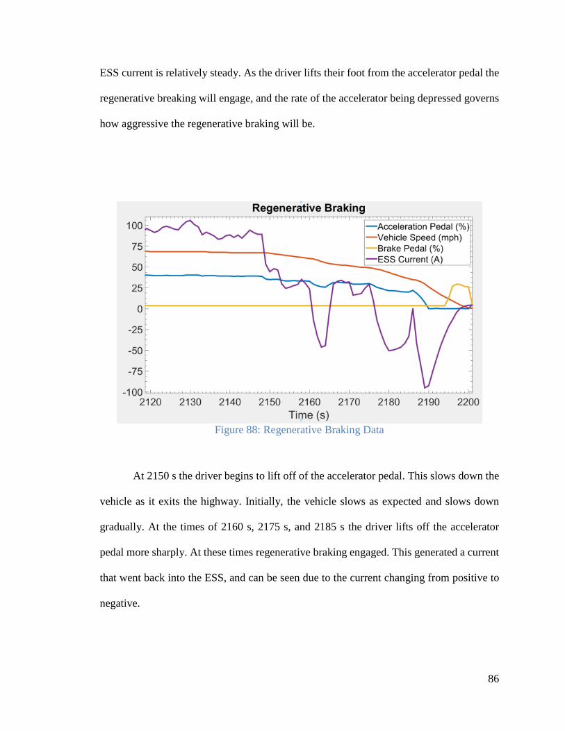
ESS current is relatively steady. As the driver lifts their foot from the accelerator pedal the
regenerative breaking will engage, and the rate of the accelerator being depressed governs
how aggressive the regenerative braking will be.
Figure 88: Regenerative Braking Data
At 2150 s the driver begins to lift off of the accelerator pedal. This slows down the
vehicle as it exits the highway. Initially, the vehicle slows as expected and slows down
gradually. At the times of 2160 s, 2175 s, and 2185 s the driver lifts off the accelerator
pedal more sharply. At these times regenerative braking engaged. This generated a current
that went back into the ESS, and can be seen due to the current changing from positive to
negative.
86

Up until 2185 s and these three regenerative braking events the vehicle the vehicle's
speed has changed from 70 mph to 14 mph in 45 s without pressing the brakes. On average,
the vehicle decelerated at a rate of 1.24 mph/s; however, during regenerative braking the
vehicle decelerated at a greater rate. This is especially seen at the time of 2185 s. At this
point, the driver lifts off the accelerator pedal completely, 0% accelerator pedal pressed,
from about 25%.This commands the greatest regenerative event represented on the above
plot, and causes the vehicle to decelerate at 2.18 mph/s. At 14 mph the driver finally presses
the brake to stop at the traffic light. This improves consumer acceptability by enabling the
driver to essentially control the vehicle's acceleration and deceleration with the accelerator
pedal. This makes it so brakes are used for the final stopping of the vehicle, or for when
extra braking is needed for safety. Since the brakes do not to be used as much, the life of
the brakes will be extended.
8.5.4 Side Skirts Aero Test
Figure 89 and Figure 90 shows the data collected during a aerodynamic test
performed on Interstate 95 near Daytona Beach. The test was performed on a 3.2 mile
stretch of the interstate, and two seperate tests were performed. Each test consisted of
driving the vehicle north bound on I-95, the vehicle gets off the highway, and then drives
south bound to return to the starting location. Speed was maintained at 70 mph as much as
possible, but was reduced if needed depending on traffic conditions to maintain safety. Test
one was performed without side skirts installed on the vehicle, and test 2 was performed
with the side skirts installed.
87

Figure 89: Aero Test No Side Skirts
+ Figure 90: Aero Test with Side Skirts
By averaging the currents from each test, it was found that having the side skirts
installed on the vehicle generated more drag. This extra drag resulted in a 2 A increase of
current with the side skirts on compared to having the skirts off. Due to the extra current
88

needed being fairly small, the range of the vehicle was not impacted. More testing will be
performed to validate the viability of the side skirts.
8.6 HV Distribution Box Design
To aid the team in component calibration and testing for EcoCAR 3. A HV demo
box has been designed specifically for bench testing of HV components within the lab. The
demo box will also serve as a tool to teach students HV safety and good practices. Figure
91 through Figure 98 shows how to properly prepare the HV cable with shielding. In order
to avoid a short between the main copper conductor and the shielding it is important to take
proper measurements for proper separation. Rule of thumb for arc distance of a given
voltage is 3 MV/m. Using this rule, 3 kV needs at most a 1 mm air gap to be able to jump.
89

Figure 91: HV Cable step 1
Figure 92: HV Cable step 2
Figure 93: HV Cable step 3
Figure 94: HV Cable step 4
Figure 95: HV Cable step 5
Figure 96: HV Cable step 6
Figure 97: HV Cable step 7
Figure 98: Cable Ends
Heat shrink is used on the HV cables to secure the shielding and insulation. If heat
shrink is not used the insulation will pull back on the cable exposing the shielding
underneath. The shielding will also fray if the ends are not secured with heat shrink.
Figure 99 through Figure 106 depicts the main components for the HV distribution
box. The main body is an electrically rated plastic enclosure with a mounting plate. The
plate is used to secure the hardware installed in the box, and the plate will also act as a
grounding plate. Copper shielding is utilized with the cable glands to allow continuity
between all of the HV cables attached to the box. Plexiglas is used in order to add safety
and separation between HV and GND. Fiberglass standoffs, made by Glastic, are also used
to insulate the HV bus bars.
90

Figure 99: HV Hardware
Figure 100: Plexiglas
Figure 101: Separators
Figure 102: Copper
Shielding
Figure 103: GND Plate
Figure 104: Enclosure
Figure 105: Gland Apart
Figure 106: Gland
Together
Figure 107 through Figure 115 details the actual build process. Holes are drilled
through the box and copper mesh to allow the cable glands to be installed. First, the copper
mesh is inserted into the box. The GND plate is then installed, followed by the Plexiglas
mold. The standoffs are then bolted into place to hold everything together. The HV fuse
and buss bars are installed and bolted into place. With the main hardware in place, the cable
glands can now be installed. The HV cables are inserted through the glands and bolted to
the buss bars. The shielding is left bare on small sections of the cables to allow the shield
91

to contact the cable gland insert. The HV test connector and HVIL micro switch are then
installed. Finally, Kapton tape is used to add insulation to all conductors.
Figure 107: Shielding in
Box
Figure 108: Plate with
Hardware
Figure 109: Glands
Installed
Figure 110: Cables Installed
Figure 111: Test Conn. &
HVIL
Figure 112: Box Insulated
Figure 113: Box Labels 1
Figure 114: Box Labels 2
Figure 115: Box Labels 3
The HV test connector, Figure 116, will allow for measurements to be taken, and
will also be used to test for isolation and ground faults. To add an extra layer of safety, A
HVIL micro switch is used to prevent the HV box from being energized.
92

Figure 116: HV test Connector and HVIL Micro Switch
The completed HV distribution box can be seen in Figure 117.
Figure 117: HV Box Complete
93

8.7 HV Simulation
Table 9 gives the values calculated with a Matlab script. Due to the size of this
script it is not included within this paper. These calculated values are used in the Simulink
model of the high voltage bus. By using these values the model is able to more precisely
estimate the voltage ripple and resonant frequency. The resonant frequency is also
calculated in the Matlab script. This value is more of an estimate for the system since it
does not take in consideration the dynamics of the bus. This value is used to help zero in
on the real resonant frequency by adjusting the output frequency of the pulse generators in
the inverters. The goal of this simulation is to find these characteristics during a worst case
scenario; therefore, the model tries to match what the high voltage bus will see during a 0
to 60 acceleration of the vehicle. This is where the most stress is exerted on the high voltage
bus.
Table 9: Simulation Calculated Characteristics Total Wire Capacitance 0.37 nF Total Load Capacitance 953.01 uF Total System Capacitance 953.01 uF Total System Inductance 0.13 uH Res Frequency of ESS branch 4964.14 Hz Res Frequency of BRUSA branch 119.47 Hz Res Frequency of IMG Generator branch 7.27 Hz Res Frequency of IMG Motor branch 7.27 Hz Res Frequency of HVAC branch 29.28 Hz HVAC Inductance 1.18 uH Inverter Inductance 1.04 uH ESS Inductance 6.89 uH BRUSA Inductance 0.22 uH Res Frequency of system 138.64 Hz
94

Figure 118, Figure 119, and Figure 120 shows the results when running the
simulation with the inverter pulse generator commanded at 12 kHz. At this frequency the
voltage ripple of the bus is seen to be 8 V peak to peak. Most high voltage components can
handle a voltage ripple of 25 V peak to peak; therefore, 8V is well within acceptable bounds
for the bus. The power spectral density block, Figure 118, also shows the frequencies seen
on the bus. This reading is in radians/second. When converted, divide rad/sec by 2π, the
frequency is found to be 12 kHz. This is the same frequency as the output of the pulse
generator, so this 12 kHz is not the resonant frequency. To find the resonant frequency the
frequency needs to be changed in the pulse generator, and the spectral analyzer, Figure
120, and PSD block, Figure 118, are observed. As the frequency on the bus approaches the
resonant frequency the power of the signal at the output frequency and the amplitude of
the voltage ripple will increase. When the signal power and voltage amplitude reach a
maximum the resonant frequency can be found.
Figure 118: Power Spectral Density 12 kHz
95

Figure 119: DC Bus Voltage 12 kHz
Figure 120: Spectrum Analyzer 12 kHz
96

The Simulation is not able to perform a frequency sweep across a range of
frequencies. This is caused by the nature of the PSD and spectrum analyzer blocks. Due to
this, the simulation has to be run for each frequency of interest. The simulation began at 12
kHz, and then a broad range of frequencies are chosen above and below 12 kHz. As the
frequency decreased from 12 kHz the power a voltage ripple increased, while the power
and voltage ripple decreased with frequencies above 12 kHz. This shows that the resonant
frequency is below 12 kHz. The frequency was then decreased by 1000 until a peak was
seen and then the signal power fell. This occurred at 1000 Hz. The frequency was then
slowly decreased until the absolute peak was seen. Figure 121, Figure 122, and Figure 123
shows the data taken at the true resonant frequency of the high voltage bus at 911 Hz. At
911 Hz the signal power is at 54 dBm versus 30 dBm at 12 kHz, and the voltage ripple at
911 Hz is 60 V peak to peak versus 8 V peak to peak. At 60 V peak to peak, there is a
definite certainty of component damage occurring. Specifically, the bulk capacitors will be
damaged preventing the voltage from being properly smoothed.
Figure 121: Power Spectral Density 911 Hz
97

Figure 122: DC Bus Voltage 911 Hz
Figure 123: spectrum Analyzer for 911 Hz
Since inverters for electric vehicles typically switch at higher frequencies between
1 and 12 kHz the 911 Hz resonant frequency should not be a problem to avoid. Even better,
98

in dealing with inverters for EcoCAR 2, 12 kHz is where manufactures seem to shoot for
with their inverters. It is currently not known what exact frequency is being used for the
Bosch IMG inverters being used on the ERAU EcoCAR 3 vehicle; however, due to the
resonant frequency being relatively low it should not cause an issues, or need any major
modifications.
9. Conclusion
At the end of EcoCAR 2 Y2 the vehicle was electrically in very bad shape. The HV
systems were in the vehicle, and for the most part in good working order. The low voltage
systems were not in good shape. The vehicle could not spin the wheels, the engine was
never wired, an SCR system was not even designed, the ESS was not capable of being
charged, and there were numerous wiring mistakes throughout the vehicle. There was an
enormous amount of work to be done in order to get a properly functioning vehicle, but
with the help of the ERAU team we were able to get a running vehicle. The team started at
13th place out of 15, and at the end of EcoCAR 2 Y3 we had taken 4th place. The quality of
the teams work truly showed. Not only were we able to complete the needed electrical
system implementation, but data was also able to be taken that was used to make systems
run more efficiently. This was a feat that had never previously been accomplished. For
EcoCAR 3 a high voltage distribution box and high voltage simulation were designed and
built. The HV distribution box will be beneficial in bench testing HV components off the
vehicle. This will allow the team to test and characterize HV components before they are
installed in the vehicle. This will both save time and valuable resources. The HV simulation
99

will allow the team to better understand the HV system in the vehicle as a whole. Instead
of hoping the system will work the team will be able to have confidence in their design by
using the simulation to understand how the high voltage will react during vehicle operation.
If a potential problem is observed, the team can take action and prevent a potential future
issue.
10. Future work
The EcoCAR 2 vehicle has been built and the team is moving all work to the
EcoCAR 3 2016 Chevrolet Camaro. Because of this, the bulk of the future work should
focus on improving the HV distribution box and HV simulation. The HV distribution box
should be used as a tool for teaching high voltage safety and best building practices. The
box can also have added circuits installed to test multiple components at once, and have
extra data collecting instrumentation added for testing purposes. The HV simulation will
need to have the components better characterized as more data is received for all the
components. This will be especially true for the Bosch IMG inverters the team will be
using. The inverters will cause the most stress on the high voltage bus; therefore, it is very
important that the team understands the inverters. The more information added to the model
will give the team the added benefit of understanding any potential issues during vehicle
operation. The vehicle wiring portion of this thesis should be used as a guide for proper
wiring and system design. Students new to the electrical team specifically will benefit from
this thesis for proper wiring techniques. Vehicle instrumentation should be added into the
EcoCAR 3 vehicle wiring. There was little time to implement this into the EcoCAR 2
100

vehicle, but it would have greatly improved data collection and troubleshooting on the
vehicle. Extra sensors for taking voltage, current, and temperature measurements will be
especially beneficial for vehicle testing and optimization of systems. This can be
implemented on both the low voltage and high voltage vehicle systems; although, great
care towards safety in the high voltage sensor instrumentation will need to be taken. Break
out boxes could also be designed to plug in-line between a wiring harness and component
for taking data and testing.
101

11. Bibliography
[1] EcoCAR 2, "About EcoCAR 2 | EcoCAR 2: Plugging In to the
Future," EcoCAR 2, 2011. [Online]. Available:
http://www.ecocar2.org/about-ecocar2.
[2] C. Rowe, I. Demirkiran, D. Bonderczuk and P. Currier, "An
Approach to Enhance the Efficiency and Consumer Acceptability of a Series
Plug-in Hybrid Vehicle," SoutheastCon 2015, pp. 1-7, 2015.
[3] "Chaohui Liu; Jiabin Wang; Colombage, K.; Gould, C.; Sen, B.;
Stone, D., "Current ripple reduction in 4kW LLC resonant converter based
battery charger for electric vehicles," in Energy Conversion Congress and
Exposition (ECCE), 2015 IEEE , vol., no., pp.60".
[4] W. Liu, Introduction to Hybrid Vehicle System Modeling and
Control, New Jersey: Wiley, 2013.
[5] R. Dorf, The Electrical Engineering Handbook, CRC PRESS, 1993.
[6] "Karvonen, Andreas; Thiringer, Torbjorn, "Co-Simulation and
Harmonic Analysis of a Hybrid Vehicle Traction System," in Vehicle Power
and Propulsion Conference (VPPC), 2015 IEEE , vol., no., pp.1-6, 19-22
Oct. 2015".
[7] "Okura, K., "Development and Future Issues of High Voltage
Systems for FCV," in Proceedings of the IEEE , vol.95, no.4, pp.790-795,
April 2007".
102

[8] "Anwar, M.N.; Gleason, S.E.; Grewe, T.M., "Design considerations
for high-voltage DC bus architecture and wire mechanization for hybrid and
electric vehicle applications," in Energy Conversion Congress and
Exposition (ECCE), 2010 IEEE , vol., no., pp.877-8".
[9] N. T. STANDARD, "CRIMPING, INTERCONNECTING
CABLES, HARNESSES, AND WIRING," National Aeronautics and Space
Administration, 2011.
[10] "GM Upfitter Integration: Electrical Best Practices," 2015. [Online].
Available:
https://www.gmupfitter.com/files/media/photo/623/New_Elect_BP_05_27_
15.pdf. [Accessed 2015].
[11] National Aeronautics and Space Administrator, "NASA
Workmanship Standards," [Online]. Available:
http://workmanship.nasa.gov/lib/insp/2%20books/frameset.html. [Accessed
2015].
[12] T. V. Johnson, "Diesel Emissions in Review," SAE International
Journal of Engines, vol. 4, no. 1, pp. 143-157, 2011.
[13] T. V. Johnson, "Vehicular Emissions in Review," SAE International
Journal of Engines, vol. 7, no. 3, pp. 1207 - 1227, 2014.
[14] BOSCH, Automotive Handbook, Robert Bosch GmbH, 2011.
[15] "SAE J1772," Wikimedia Foundation, 1 November 2015. [Online].
Available: https://en.wikipedia.org/wiki/SAE_J1772.
103

[16] D. Barsotti and S. Boetcher, "OPTIMIZING JETS FOR ACTIVE
WAKE CONTROL OF GROUND VEHICLES," Proceedings of the ASME
2013 International Mechanical Engineering Congress & Exposition IMECE
2013. San Diego..
[17] C. P. Rowe II, D. Bonderczuk, C. M. Rowe, Y. Meng and P. N.
Currier, "Refinement and Optimization of a Series Plug-In Hybrid Electric
Vehicle with a B20 Bio-Diesel Generator as Part of EcoCAR 2: Plugging
into the future," 2014.
[18] A. D'Hooge, R. Palin and S. Johnson, "The Aerodynamic
Development of the Tesla Model S - Part 2: Wheel Design Optimization,"
2012. SAE 2012 World Congress & Exhibition. Detroit..
[19] H. Khalifi, "Hybrid electric power system validation through
parameter optimization," Embry-Riddle Aeronautical University, Daytona
Beach, 2015.
104