AN APPROACH TO ANALYZING HISTOLOGY

SEGMENTATIONS USING SHAPE DISTRIBUTIONS

A Thesis

Submitted to the Faculty

of

Drexel University

by

Jasper Z. Zhang

in partial fulfillment of the

requirements for the degree

of

Master of Science

in

Computer Science

March 2008

© Copyright 2008 Jasper Z. Zhang. All Rights Reserved.

i

ACKNOWLEDGMENTS

The U.S. Army Medical Research Acquisition Activity, 820 Chandler Street, Fort Detrick, MD 21702-5014 is the awarding and administering acquisition office. This investigation was partially funded under a U.S. Army Medical Research Acquisition Activity; Cooperative Agreement W81XWH 04-1-0419. The content of the information herein does not necessarily reflect the position or the policy of the U.S. Government, the U.S. Army or Drexel University and no official endorsement should be inferred. Any opinions, findings, and conclusions or recommendations expressed in this material are those of the author.

ii

TABLE OF CONTENTS

LIST OF TABLES .............................................................................................................iv

LIST OF FIGURES ........................................................................................................... v

LIST OF EQUATIONS ................................................................................................ viii

ABSTRACT ......................................................................................................................... ix

1. INTRODUCTION ...................................................................................................... 1

1.1. Pathology and histology ...................................................................................... 1

1.2. Shape distributions ............................................................................................... 3

1.3. Previous works ...................................................................................................... 4

1.4. Our goal .................................................................................................................. 6

1.5. Our process............................................................................................................ 7

1.6. Thesis structure ..................................................................................................... 9

2. COMPUTATIONAL PIPELINE ............................................................................ 9

2.1. Segmentation ...................................................................................................... 13

2.2. Shape distribution extractions ......................................................................... 15

2.2.1. Inside radial contact.............................................................................. 17

2.2.2. Line sweep .............................................................................................. 19

2.2.3. Area ......................................................................................................... 23

2.2.4. Perimeter ................................................................................................ 25

2.2.5. Area vs. perimeter ................................................................................. 26

2.2.6. Curvature ................................................................................................ 27

iii

2.2.7. Aspect ratio ............................................................................................ 30

2.2.8. Eigenvector ............................................................................................ 33

2.3. Computational Performance ................................................................................

2.4. Distribution analysis .......................................................................................... 35

3. DATA PROCESSING ............................................................................................. 37

3.1. Preprocess ........................................................................................................... 37

3.2. Post process ........................................................................................................ 41

3.3. Pre-segmentation dependencies ...................................................................... 48

4. ANALYSIS ................................................................................................................. 50

4.1. Earth mover’s distance ..................................................................................... 51

4.2. Shape distribution sub-regions ........................................................................ 53

4.3. Information retrieval analysis .......................................................................... 56

5. CONCLUSIONS ....................................................................................................... 34

5.1. Conclusion .......................................................................................................... 67

5.2. Future work ........................................................................................................ 68

APPENDIX A: BEST PERFORMANCE ................................................................. 70

APPENDIX B: ONLINE RESOURCES ........................................................................

LIST OF REFERENCES ............................................................................................... 77

iv

LIST OF TABLES

Number Page

Table 2-1 Performance of all metrics .................................................................................. 34

Table 3-1 Data preprocess ..................................................................................................... 39

Table 3-2 Histogram binning multipliers ............................................................................ 41

Table 3-3 The before and after of the data range after post processing ....................... 42

Table 3-4 The before and after of the bucket count after post processing .................. 43

Table 3-5 Shape distribution ranges for all metrics........................................................... 47

Table 4-1 Best performing windows for Grade 1 ............................................................. 61

Table 4-2 Best performing windows for Grade 2 ............................................................. 63

Table 4-3 Best performing windows for Grade 3 ............................................................. 65

v

LIST OF FIGURES

Number Page

Figure 1-1 Medical process ....................................................................................................... 2

Figure 1-2 A broad overview of the computational pipeline. ............................................ 6

Figure 1-3 Segmentation process ............................................................................................ 8

Figure 2-1. Input images ........................................................................................................ 12

Figure 2-2. Segmentation screenshot ................................................................................... 14

Figure 2-3. Output segmentations ....................................................................................... 15

Figure 2-4. Concept of inside radial contact ...................................................................... 17

Figure 2-5. Potential error in distance transform using square flood fill ...................... 18

Figure 2-6. Implementation of square flooding in inside radial contact ....................... 19

Figure 2-7. Conceptual definition of line sweep ................................................................ 20

Figure 2-8. Implementation of visiting boundary pixel for line sweep ......................... 20

Figure 2-9. Implementation of look at in line sweep ........................................................ 21

Figure 2-10. Implementation of area ................................................................................... 24

vi

Figure 2-11. Concept of area and perimeter....................................................................... 24

Figure 2-12. Implementation of interface detection in perimeter .................................. 26

Figure 2-13. Conceptual definition of curvature ............................................................... 28

Figure 2-14. Implementation of curvature ......................................................................... 29

Figure 2-15. Conceptual definition of aspect ratio ............................................................ 30

Figure 2-16. Definition of eigen systems ............................................................................ 31

Figure 2-17 Histogram of inside radial contact and eigenvector .................................... 36

Figure 3-1 Segmentation error with large tubular formations ........................................ 40

Figure 3-2 Example of inside radial contact’s histogram ................................................. 45

Figure 3-3 Example of curvature’s histogram .................................................................... 46

Figure 3-4 Multiple segmentations at 10x magnification ................................................. 49

Figure 4-1 Regions of good separations ............................................................................. 55

Figure 4-2 Sub-region sliding window ................................................................................. 55

Figure 4-3 K nearest neighbor .............................................................................................. 56

Figure 4-4 Maximum performance value of Grade 1 in respect to k-values. .............. 60

vii

Figure 4-6 Grade 1 best window .......................................................................................... 61

Figure 4-8 Maximum performance value of Grade 2 in respect to k-values. .............. 62

Figure 4-12 Grade 2 best window ........................................................................................ 64

Figure 4-14 Maximum performance value of Grade 3 in respect to k-values. ............ 65

Figure 4-15 Grade 3 best window ........................................................................................ 66

viii

LIST OF EQUATIONS

Number Page

Equation 2-1 Level set curvature.......................................................................................... 28

Equation 2-2 Definition of covariant matrix in terms of a ROI’s pixels’ x and y coordinate ................................................................................................................................. 32

Equation 3-1 Mumford-Shah framework ........................................................................... 38

Equation 4-1 Precision measure ........................................................................................... 58

Equation 4-2 Recall measure ................................................................................................. 59

Equation 4-3 F-measure ......................................................................................................... 59

ix

ABSTRACT

AN APPROACH TO ANALYZING HISTOLOGY

SEGMENTATIONS USING SHAPE DISTRIBUTIONS

Jasper Zhang

David E. Breen, Ph. D.

Histological images are the key ingredients in medical diagnosis and prognosis in

today’s medical field. They are imagery acquired by analysts from microscopy to

determine the cellular structure and composition of a patient’s biopsy. This thesis

provides an approach to analyze the histological segmentation obtained from

histological images using shape distributions and provides a computationally feasible

method to predict their histological grade.

This process provides a way of generating suggestions using segmented images in

a way that is independent of the segmentation process. The process generates

histograms for each image that describes a set of shape distributions generated from

eight metrics that we have devised. The shape distributions are extracted from a

learning set that the user provides. The shape distributions are then analyzed by

querying a classification for each case using K-nearest-neighbor. The quality of the

classifications is measured by a composite measure composed of precision and recall

based on the query.

1

C h a p t e r 1

INTRODUCTION

Computational histology is a new and emerging field in medical imaging in

today’s world and for a good reason. The demand for histological analysis is becoming

increasingly large while the number of providers of such a service has stayed about the

same [54] [3]. To cope with this increasing problem of consumer vs. producer, more

and more pathologists have turned to automating their work through computational

histology [53]. But as research has shown, it is not easy to extract meaningful

information from a histological slide [7]. This paper proposes a way to acquire

information from a histological segmentation and suggest histological grading for new

cases.

1.1 Pathology and histology

Pathology (also known as pathobiology), under the definition of American

Heritage Science Dictionary, is “the scientific study of the nature of disease and its

causes, processes, development, and consequences.” What that means for the

everyday person is that pathologists are the people that can definitively say what

disease, if any, we have and what the diagnosis and prognosis of the disease are. The

pathologist is one of the crucial specialists in treating a patient who has a disease.

2

Though it is not always like this, the process of patient care can be generalized into

Figure 1-1.

Figure 1-1 Medical process

As we can see from the diagram, a pathologist doesn't come into the picture in

the lab process until after a biopsy or sample of the patient is extracted. This means

the pathologist is only dealing with samples of the patient, not inferring anything from

3

just symptoms. So what this brings up is that pathologists are really dealing with

histology when they do their job. Histology, under the definition of American

Heritage Science Dictionary, is “the branch of biology that studies the microscopic

structure of animal or plant tissues.” This definition allows for some development on

the computational front mainly due to the key phrase “microscopic structure”. What

that implies is that it is a study of the shapes and geometry of an image. This is what

allows us to consider our work in this thesis.

The information that a pathologist gains from a histological study allows them to

generate diagnosis and prognosis for the patient. This diagnosis can fall under many

different histological grades. The histological grades are determined by an existing

heuristic specifically designed for the disease and allow the pathologist to easily come

up with a diagnosis that is fitting for the patient.

1.2 Shape distribution

The main objective of this thesis is to develop a computational method that is

capable of discriminating between histological images based on their geometry. This

objective can only be achieved by giving each image a set of metrics that allows them

to be compared. The obvious problem of this operation is the comparison itself.

How can you compare a dataset, such as an image, with another in a meaningful way?

Shape distribution gives a suitable solution to this problem. A shape distribution is a

signature of the image in a fashion that allows for quantitative comparisons.

4

A shape distribution of an image is a sample of that image based on the

application of a shape function that measures the local geometric properties and

captures some global statistical property of an object. What this means is that the

shape distributions will represent the image in a way that describes the statistical

occurrences resulting from a shape function. That shape function can be anything; it

can be passing a line through the image, how likely you are to sample a certain color

when a random pixel is picked, how big each area of certain criteria is, etc.

The objective of this thesis is to build shape functions (that we call metrics) that

can generate shape distributions that can aid in classifying histological segmentations.

The helpfulness or success of a shape function is described by how well it can identify

similar shapes as similar and how well it can identify dissimilar shapes as dissimilar

while all at the same time be able to operate independently of any reorientation and

repositioning that can happen to the image [42].

1.3 Previous work

Most of the work done in this area in the past has been focused mostly on

segmentation. A majority of the reason why it hasn’t moved on is based on the fact

that biological images are still a challenge to segment. It is one of the hardest

problems facing computer vision and image analysis to this day [34]. Part of the

reason is that due to the over abundance of information it is hard to segment images

from medical domain to medical domain using the same process [31] [43]. Many ad

5

hoc techniques were developed for problem specific application to overcome this

problem [7] [41] [45].

Due to the problem of segmenting the images many experts have used

information on geometry and other analysis-based information to help segment the

image [56] [14]. This leads to a hybrid approach between analysis and segmentation

that has both happening at the same time. This leads to a solution to analysis and

segmentation at the end of the whole process. This approach, too, is limited to a

specific problem domain.

In recent years many experts have given up on trying to fully automate

segmentation and reverted to using only semi-automatic techniques [40] [37] [38] [19]

[33]. These techniques involve having human intervention as well as a mix of

techniques stated above. Thought these techniques involve human intervention, they

will almost always guarantee a satisfactory result for the user, at least in areas that the

user is concerned with. This approach introduces a new problem of human computer

interaction with the need of a well defined user interface that is easy and fast to use

[36] [46].

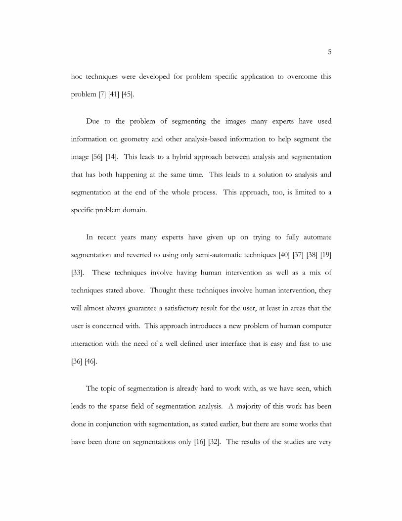
The topic of segmentation is already hard to work with, as we have seen, which

leads to the sparse field of segmentation analysis. A majority of this work has been

done in conjunction with segmentation, as stated earlier, but there are some works that

have been done on segmentations only [16] [32]. The results of the studies are very

6

data-centric. The analysis themselves can only be as good as the segmentations

themselves.

1.4 Our goal

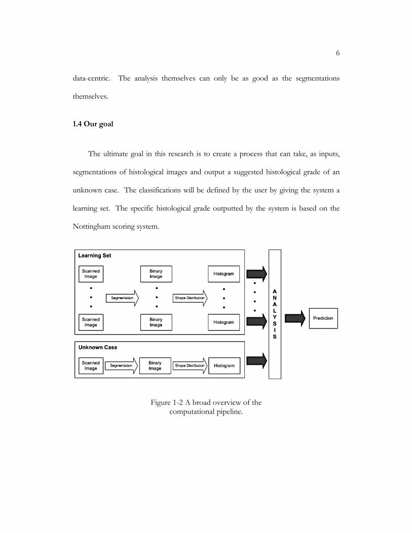
The ultimate goal in this research is to create a process that can take, as inputs,

segmentations of histological images and output a suggested histological grade of an

unknown case. The classifications will be defined by the user by giving the system a

learning set. The specific histological grade outputted by the system is based on the

Nottingham scoring system.

Figure 1-2 A broad overview of the computational pipeline.

7

This research also explores the usefulness of specific shape functions when

applied to histology segmentations. Even if we don’t achieve the ultimate goal of

suggesting histological grade, we would like to at least be able to state a quantitative

success of a given shape function with the given histology segmentations.

1.5 Our process

The work in this thesis falls under the last category in the previous work section.

Our process generates analysis based on segmentations, not analysis parallel to

segmentation. The overall process that we propose is shown in Figure 1-2. This

process takes in a learning set to define classification groups and an unknown case or

set of unknown cases whose histological grade will be predicted. What this process

involves is to first digitize the slides into digital images. The digital images are then

segmented to produce binary images that represent only the background and the areas

of interest. The binary images are then transformed into histograms that represent the

shape distribution produced by applying geometric measures to the images. The

distributions are then analyzed and used to suggest the classification of the unknown

cases.

8

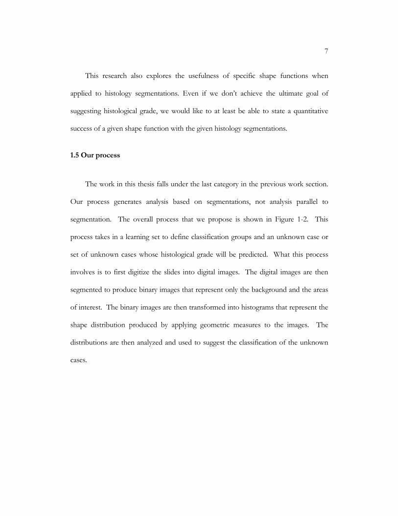
Figure 1-3 Segmentation process

The first stage of the pipeline is the digitization of the slides (Figure 1-3). The

slides are given to us as a set of Hematoxylin and Eosion (H&E) stained slides. The

slides are then scanned one sub-region at a time to ensure maximum detail and

resolution. The individual images are then stitched together into a single large image

that represents the slide.

The next stage in the process is the segmentation stage where the raw image is

taken and a binary image will be the output. The process will first take an image and

convert it into our optimal color space and a user interface will guide the user in

helping the system determine the proper segmentation of the image. The user “trains”

the system based on the definition of cells, as we are only interested in studying the

morphology of cells within our slides in this study.

9

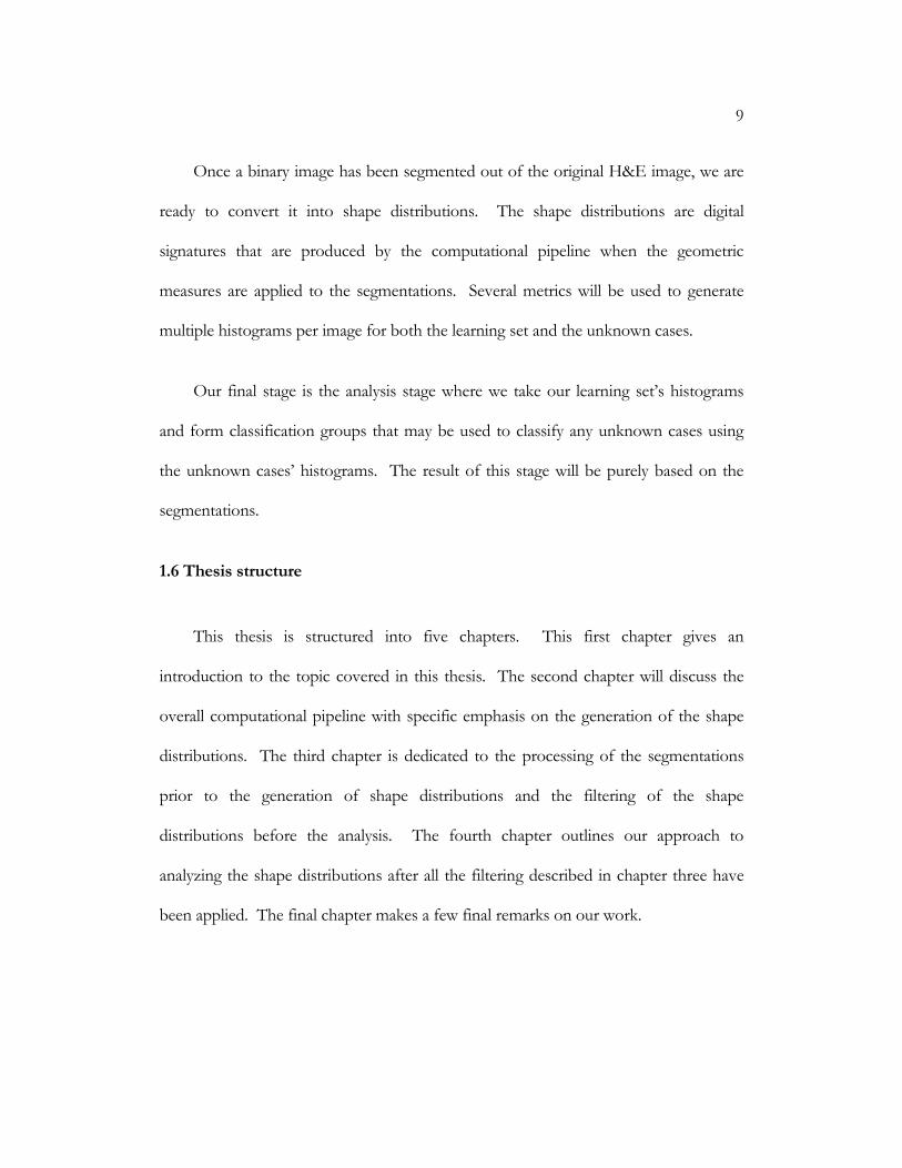
Once a binary image has been segmented out of the original H&E image, we are

ready to convert it into shape distributions. The shape distributions are digital

signatures that are produced by the computational pipeline when the geometric

measures are applied to the segmentations. Several metrics will be used to generate

multiple histograms per image for both the learning set and the unknown cases.

Our final stage is the analysis stage where we take our learning set’s histograms

and form classification groups that may be used to classify any unknown cases using

the unknown cases’ histograms. The result of this stage will be purely based on the

segmentations.

1.6 Thesis structure

This thesis is structured into five chapters. This first chapter gives an

introduction to the topic covered in this thesis. The second chapter will discuss the

overall computational pipeline with specific emphasis on the generation of the shape

distributions. The third chapter is dedicated to the processing of the segmentations

prior to the generation of shape distributions and the filtering of the shape

distributions before the analysis. The fourth chapter outlines our approach to

analyzing the shape distributions after all the filtering described in chapter three have

been applied. The final chapter makes a few final remarks on our work.

10

C h a p t e r 2

COMPUTATIONAL PIPELINE

The computational pipeline that we are working with starts with a scanned section

of a biopsy. We make no assumptions about the color corrections or the

magnifications of the image when it is first presented. We assume the user to be the

responsible party for assuring data coherency.

The input data must be segregated into two groups: the learning set and the

unknown case(s). The learning set will also need to be segregated into classification

groups. The classification groups will determine the set of all possible categories into

which an unknown case can be placed. The pipeline will not take into account all

subcategories that may exist within a group. If subcategories do exist within a group

then the user must define them as separate classification groups.

The user must also take into consideration at scale of which images were scanned

before processing. The scale of the image will ultimately determine the performance

of certain metrics within the shape distribution stage. More on the scale of the input

images will be explained in the analysis section of this paper.

The computational pipeline (Figure 1-2) consists of processing all input images

through the segmentation and shape distribution extraction stages before performing

11

the final classification analysis on an unknown case. This whole pipeline is modular

and can be done piecewise. Each image can be described as its own pipeline; allowing

multiple images to be computed in parallel, if the computing environment allows for

this.

The segmentation process is essentially any process that takes a raw image and

converts it into a binary image. The raw image could be binary to start out with, or

could use as many bits as necessary to describe the subject, as long as the segmentation

process knows how to handle it. The main goal of the segmentation process is to

reduce any input into two partitions per image: the regions of interest and the

background [57].

The shape distribution extraction process, which will be discussed in more detail

later on, involves multiple geometric metrics that will generate a set of shape

distributions that can describe each image, which capture geometric features in the

image. The shape distribution extraction stage depends on specified regions of interest

within a segmented image. Each metric within the extraction stage will generate its

own histogram that can be used later for analysis. Most metrics within the shape

distribution extraction stage can be computed independently of one another, allowing

for parallel computation.

12

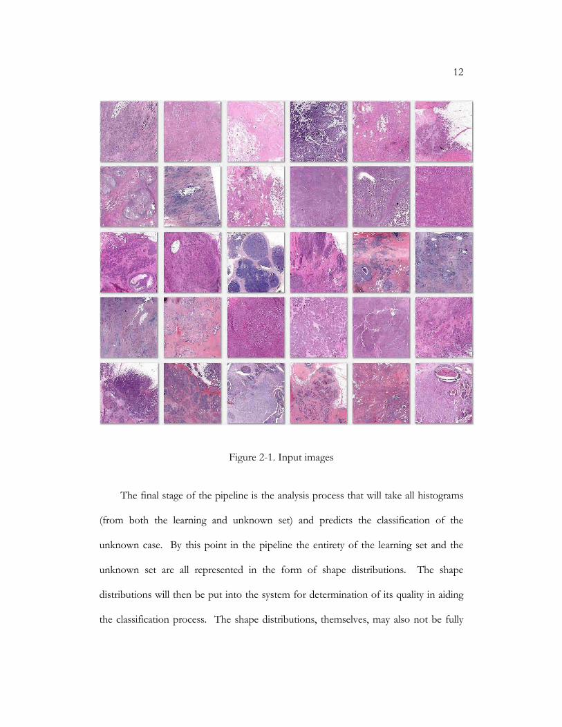
Figure 2-1. Input images

The final stage of the pipeline is the analysis process that will take all histograms

(from both the learning and unknown set) and predicts the classification of the

unknown case. By this point in the pipeline the entirety of the learning set and the

unknown set are all represented in the form of shape distributions. The shape

distributions will then be put into the system for determination of its quality in aiding

the classification process. The shape distributions, themselves, may also not be fully

13

qualified to classify either. So for example, a shape distribution could have only a

certain percentage of itself used for classification and the rest will be discarded. The

goal of this stage is to use the given shape distributions and generate the best possible

prediction.

2.1 Segmentation

The segmentation process is not the focus of this paper but to fully treat this

topic the segmentation process that was used will be described briefly. The

segmentation for this thesis has been provided to us by Sokol Petushi and the

Advanced Pathology Imaging Laboratory (Drexel University School of Medicine).

The segmentation technique that was used to generate the data for this paper was

done using a semi-unsupervised technique. It is used to extract all nucleuar structures

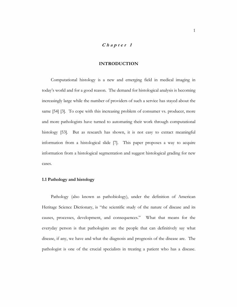
within a section of a biopsy. The images that were given to us were from breast cancer

patients ranging from histological grade of one to three with no healthy specimens

(Figure 2-1). All images were stained using the Hematoxylin and Eosion (H&E)

process. The images were all scanned in at a magnification of 10x at a pixel resolution

of 6,000 pixels2 per slide block. We then choose only one slide block out of the

numerous images acquired per slide for the segmentation process. We choose the

slide block based on what our pathologist deems to be the greatest region of interest

within the slide. Our reasoning is that no pathologist will look at everything in a whole

slide but only areas of interest within a slide.

14

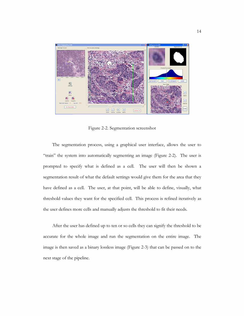
Figure 2-2. Segmentation screenshot

The segmentation process, using a graphical user interface, allows the user to

“train” the system into automatically segmenting an image (Figure 2-2). The user is

prompted to specify what is defined as a cell. The user will then be shown a

segmentation result of what the default settings would give them for the area that they

have defined as a cell. The user, at that point, will be able to define, visually, what

threshold values they want for the specified cell. This process is refined iteratively as

the user defines more cells and manually adjusts the threshold to fit their needs.

After the user has defined up to ten or so cells they can signify the threshold to be

accurate for the whole image and run the segmentation on the entire image. The

image is then saved as a binary lossless image (Figure 2-3) that can be passed on to the

next stage of the pipeline.

15

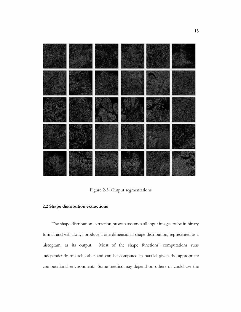
Figure 2-3. Output segmentations

2.2 Shape distribution extractions

The shape distribution extraction process assumes all input images to be in binary

format and will always produce a one dimensional shape distribution, represented as a

histogram, as its output. Most of the shape functions’ computations runs

independently of each other and can be computed in parallel given the appropriate

computational environment. Some metrics may depend on others or could use the

16

results of other metrics to optimize its own computations. Some of these decisions are

made due to computational constraints.

The shape distributions produced by applying the shape functions can be viewed

as probability density functions associated with the given image when analyzed with a

certain shape function. Each bucket, or a location in the one dimensional histogram,

represents the number of occurrences (or probability) of a measurement while using

that shape function. For instance, if we are trying to determine how many people are

age 25 in a group of people, we would bin everyone with the age of 25 to the bucket of

25. The values in each bucket represent the count of the occurrences of that value

within the image when applying the metric. So taking our example of people of age

25, our histogram would have a value of five at the location of 25 if there are five

people who are 25 years old. Taking the example further, we would have one

histogram for every demographic group that we are working with. Each histogram

will be the distribution of age in that particular group.

The metrics that we have defined and implemented for generating shape

distributions are inside radial contact, line sweep, area, perimeter, area vs. perimeter,

curvature, aspect ratio and eigenvector. The remainder of this section describes how

these shape functions have been implemented to generate shape distributions that

capture geometric features in histology segmentations.

17

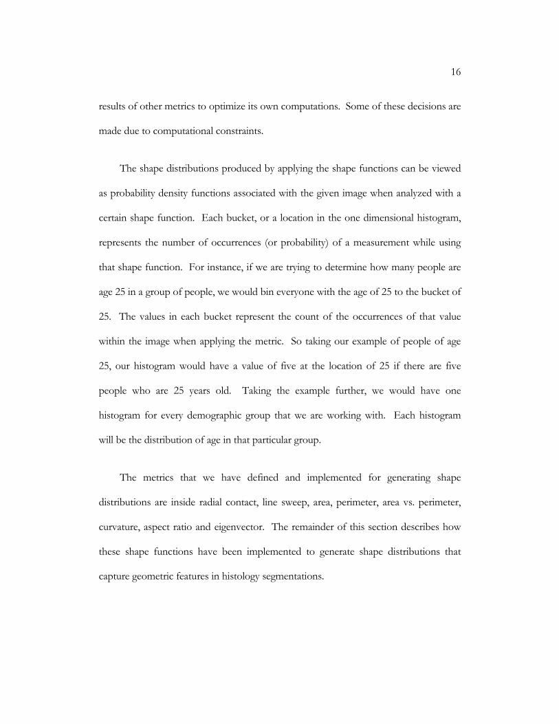
Figure 2-4. Concept of inside radial contact

2.2.1 Inside radial contact

Inside radial contact is a metric that has been used in previous works in geometric

matching [29] [18] [47]. The idea behind inside radial contact is to gain insight into the

size distribution of an image by probing it with disks. We treat each inside pixel as the

center of a disk that is used to probe the shape. The algorithm will determine the

maximum radius of a disk that can be fit inside the shape from that pixel (Figure 2-4).

This algorithm can be implemented in multiple ways but it is most efficiently

calculated using a distance field transformation of the image [49] [4]. One of the

efficiency comes from preserving some information about the image that can be used

later for other metrics, for example the curvature metric.

Methods for obtaining a distance field include passing the image through a

convolution [30] [24], solving it as a Hamilton-Jacobi equation [5], processing it with a

fast marching method [31], or applying the Danielsson distance transform [13] [28].

These approaches are good if the image size is not excessively large. In the case of our

18

dataset, the size can get prohibitively large for this approach. Most of our problems

originate back to trying to transform an image more than 10,000 pixels2.

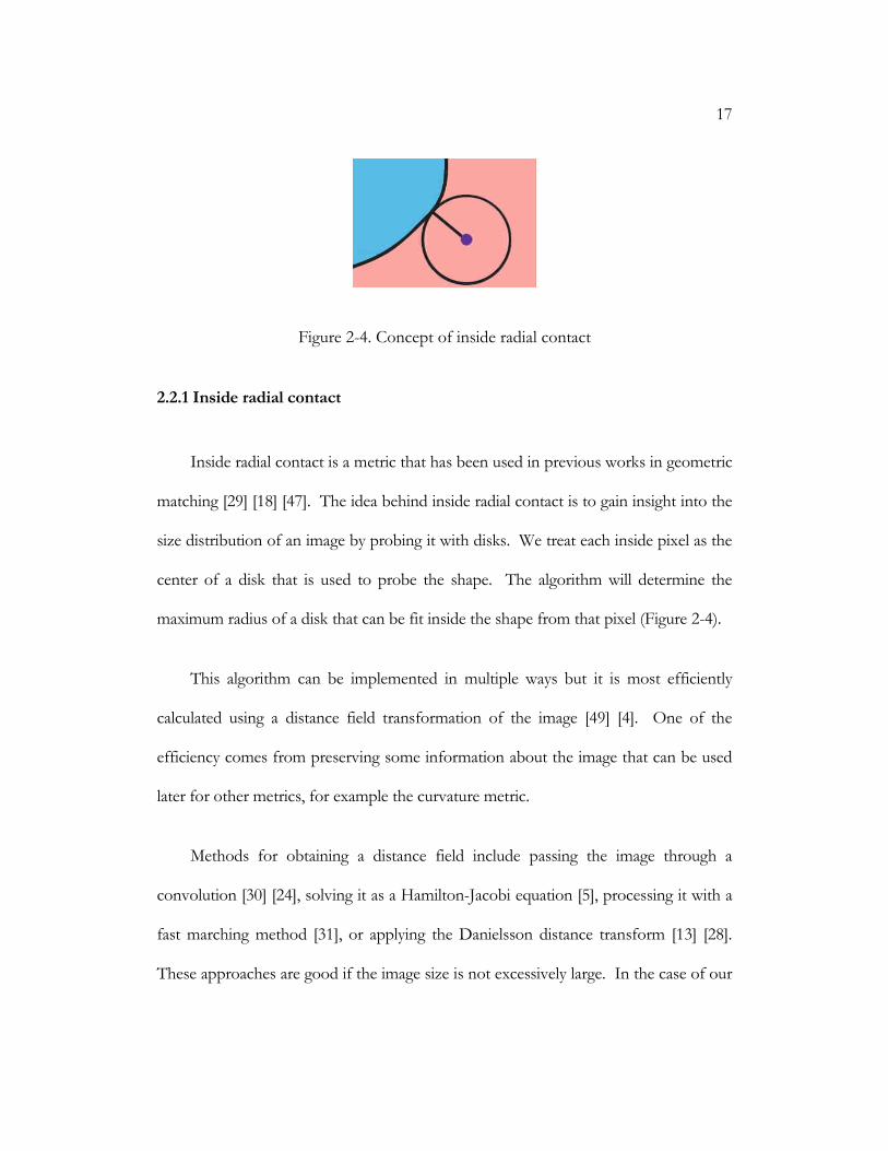
Figure 2-5. Potential error in distance transform using square flood fill

Because of our hardware issues we had to step back and approached this problem

in a temporally less efficient but spatially more efficient manner. Our approach was to

take each pixel and do a square flooding on the area, which could detect changes in the

pixel color (Figure 2-6). After it found the first pixel of changed color it will then keep

expanding past the current location, compensating for the increased distance that may

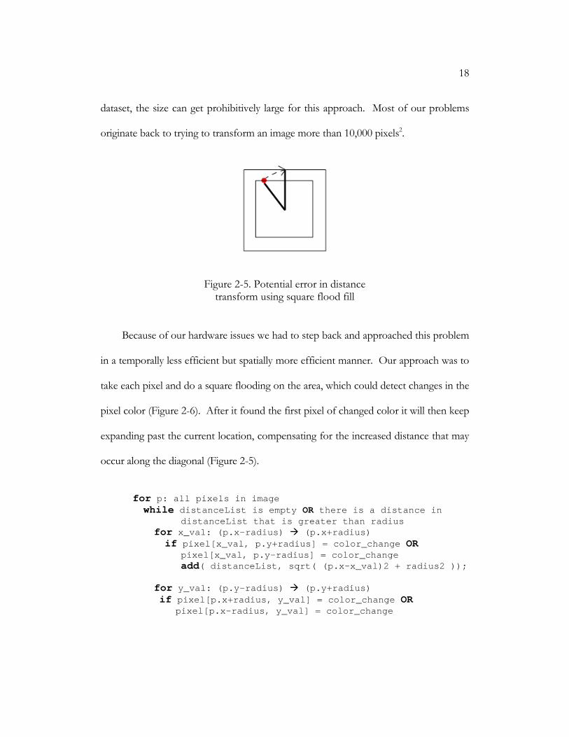
occur along the diagonal (Figure 2-5).

for p: all pixels in image while distanceList is empty OR there is a distance in distanceList that is greater than radius

for x_val: (p.x–radius) � (p.x+radius) if pixel[x_val, p.y+radius] = color_change OR pixel[x_val, p.y-radius] = color_change add( distanceList, sqrt( (p.x-x_val)2 + radius2 ));

for y_val: (p.y-radius) � (p.y+radius) if pixel[p.x+radius, y_val] = color_change OR pixel[p.x-radius, y_val] = color_change

19

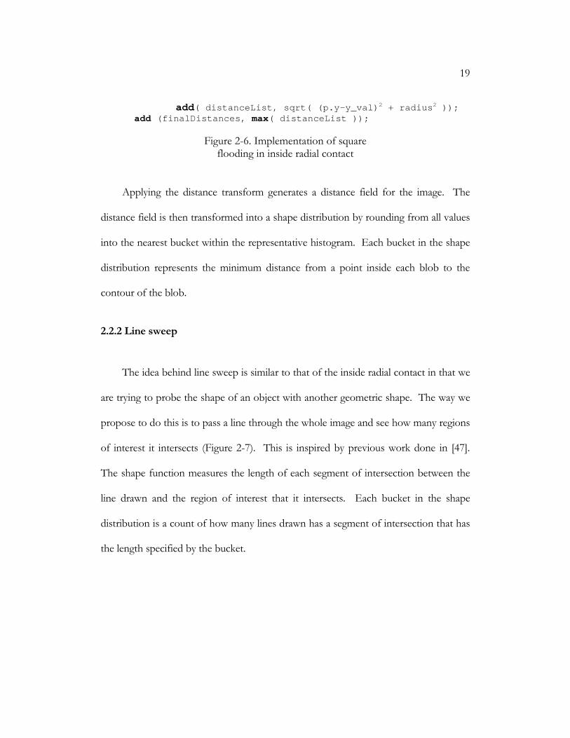
add( distanceList, sqrt( (p.y-y_val) 2 + radius 2 )); add (finalDistances, max( distanceList ));

Figure 2-6. Implementation of square flooding in inside radial contact

Applying the distance transform generates a distance field for the image. The

distance field is then transformed into a shape distribution by rounding from all values

into the nearest bucket within the representative histogram. Each bucket in the shape

distribution represents the minimum distance from a point inside each blob to the

contour of the blob.

2.2.2 Line sweep

The idea behind line sweep is similar to that of the inside radial contact in that we

are trying to probe the shape of an object with another geometric shape. The way we

propose to do this is to pass a line through the whole image and see how many regions

of interest it intersects (Figure 2-7). This is inspired by previous work done in [47].

The shape function measures the length of each segment of intersection between the

line drawn and the region of interest that it intersects. Each bucket in the shape

distribution is a count of how many lines drawn has a segment of intersection that has

the length specified by the bucket.

20

Figure 2-7. Conceptual definition of line sweep

Computationally, the metric will calculate lines from every boundary pixel of the

image to all other boundary pixels, ensuring that the start and end pixels are not the

same boundary (Figure 2-8). This guarantees that all possible lines that can be

processed are processed since the problem is symmetrical, a line going in the direction

of point A to point B will produce the same result as that going from point B to point

A.

boundary = all pixels at the edge of the image for i: 0 � size(boundary) for j: i+1 � size(boundary) if ( NOT isOnSameSideAs( boundary[i], boundary[j] ) ) shootLine( boundary[i], boundary[j] )

Figure 2-8. Implementation of visiting boundary pixel for line sweep

21

The actual line processing algorithm can be any line drawing algorithm that the

implementer chooses. The line drawing algorithm we chose to use is the Bresenham

line raster algorithm [6]. We chose it because it is fast and the most commonly used

line raster algorithm. The only difference with our approach is that instead of drawing

a pixel at every raster we do a look at function that determines if there is a transition of

colors (Figure 2-9). This keeps track of the starting and ending locations of a line

segment that is drawn contiguously through a region of interest. We compute the

Euclidean distance between the start and end locations.

LOOKAT x, y, I if I[x,y] = inside

if NOT isInside isInside = TRUE p1 = Point[x,y]

if I[x,y] == outside

if isInside incrementBucket( lengthList, distance(p1, Point[ x,y]) ) isInside = FALSE

Figure 2-9. Implementation of look at in line sweep

Another special concern is usage of image libraries. From many experiments we

have discovered that an image library that involve built in virtual swapping should be

avoided (in our case, the Image Magick API). Using this library causes problems

because this algorithm will sweep the whole entire image every iteration. So if the

library swaps in only a portion of the image at any given instance, anticipating localized

computation, it will have to clean out the whole image cache in memory repeatedly

22

every iteration. This will produce excessive over utilization of the processor and

memory bus for needless operations. This, however, requires the system to have

enough memory to store the whole image at once as well as control over the caching

of the image library API. If the system memory can’t hold the full image then it is

highly advised that the developer implement their own caching scheme that will

minimize on demand paging within each iteration. Another concern with image

libraries is that it is a good idea to avoid any that use class hierarchies and other object

oriented overhead, such as the Image Magick API [9] [12] [25]. The computation is

already extensive, taking a minimum of eight hours on a 60,000 pixel2 image; adding

object oriented overhead would drastically increase runtime.

The final computation concern of the line sweep algorithm is parallel

computation. After some experiments we have discovered that threading the line

processing procedure will not improve the computation time at all. After analyzing the

system monitor we discovered that when the whole image is in memory with a singly

threaded build, CPU utilization is always near maximum with almost no wait time for

I/O access. But when we employ a multi-threaded build that utilizes symmetric

multithreading (better known as Hyper-threading in the Intel core) the CPU utilization

of both cores dropped below 60%. From this we can infer that the main memory bus

is only able to provide enough throughput for a single core computation. Anything

more would cause I/O wait time for the process.

23

2.2.3 Area

The area metric is computationally the simplest of all metrics. It finds the area, in

pixels, of all regions of interest (defined by inside regions) within the image (Figure

2-11). Applying the area metric produces a profile of the size distribution of regions of

interest in the given image. The difference between area and inside radial contact is

that inside radial contact finds a size distribution on the pixel level whereas the area

metric finds a size distribution on the regions of interest level. The shape distribution

generated by area produces a histogram that measures the area of a complete blob.

Each bucket within the area shape distribution represents the count of blobs of the

specified area.

The implementation of the area metric is very simple in that it depends heavily on

a recursive procedure. Once it finds an inside pixel it will try to flood the area looking

for other inside pixels until it hits an outside pixel. It will do this until no more inside

pixels can be explored within the region of interest, in which case it will count the

number of pixels inside the region and bin itself into the appropriate bin and move

onto an inside pixel of the next region of interest. This implementation uses a residual

image to insure that no region of interest is binned twice. This residual image will keep

track of all pixels visited by the algorithm already. It needs to be looked at along side

the actual image simultaneously. This image can be the same size as that of the

original image, if memory allows, or it could be a block of the image. Some form of

24

book keeping is needed to make sure that the residual image matches up with the

location of the current read in the original image (Figure 2-10).

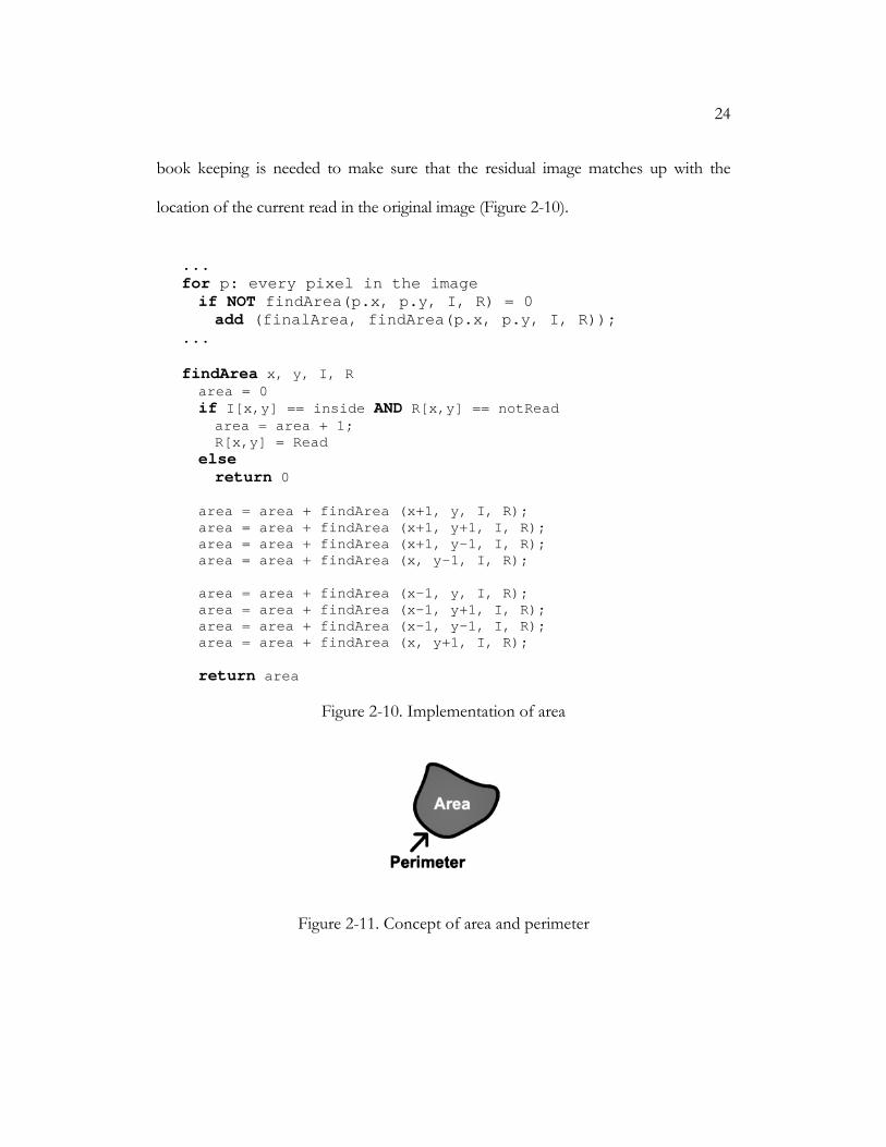
... for p: every pixel in the image if NOT findArea(p.x, p.y, I, R) = 0

add (finalArea, findArea(p.x, p.y, I, R)); ... findArea x, y, I, R

area = 0 if I[x,y] == inside AND R[x,y] == notRead

area = area + 1; R[x,y] = Read

else return 0

area = area + findArea (x+1, y, I, R); area = area + findArea (x+1, y+1, I, R); area = area + findArea (x+1, y-1, I, R); area = area + findArea (x, y-1, I, R); area = area + findArea (x-1, y, I, R); area = area + findArea (x-1, y+1, I, R); area = area + findArea (x-1, y-1, I, R); area = area + findArea (x, y+1, I, R);

return area

Figure 2-10. Implementation of area

Figure 2-11. Concept of area and perimeter

25

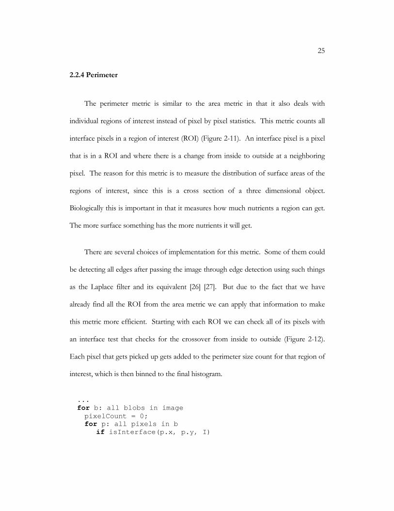
2.2.4 Perimeter

The perimeter metric is similar to the area metric in that it also deals with

individual regions of interest instead of pixel by pixel statistics. This metric counts all

interface pixels in a region of interest (ROI) (Figure 2-11). An interface pixel is a pixel

that is in a ROI and where there is a change from inside to outside at a neighboring

pixel. The reason for this metric is to measure the distribution of surface areas of the

regions of interest, since this is a cross section of a three dimensional object.

Biologically this is important in that it measures how much nutrients a region can get.

The more surface something has the more nutrients it will get.

There are several choices of implementation for this metric. Some of them could

be detecting all edges after passing the image through edge detection using such things

as the Laplace filter and its equivalent [26] [27]. But due to the fact that we have

already find all the ROI from the area metric we can apply that information to make

this metric more efficient. Starting with each ROI we can check all of its pixels with

an interface test that checks for the crossover from inside to outside (Figure 2-12).

Each pixel that gets picked up gets added to the perimeter size count for that region of

interest, which is then binned to the final histogram.

... for b: all blobs in image

pixelCount = 0; for p: all pixels in b

if isInterface(p.x, p.y, I)

26

pixelCount = pixelCount + 1; add( finalPerimeter, pixelCount ); ...

isInterface x, y, I if I[x,y] == outside return FALSE

if NOT I[x-1,y] == I[x,y]

return TRUE else if NOT I[x,y-1] == I[x,y]

return TRUE else if NOT I[x+1,y] == I[x,y]

return TRUE else if NOT I[x,y+1] == I[x,y]

return TRUE else if NOT I[x+1,y+1] == I[x,y]

return TRUE else if NOT I[x-1,y-1] == I[x,y]

return TRUE else if NOT I[x-1,y+1] == I[x,y]

return TRUE else if NOT I[x+1,y-1] == I[x,y]

return TRUE else return FALSE

Figure 2-12. Implementation of interface detection in perimeter

2.2.5 Area vs. Perimeter

Area vs. perimeter is a metric that combines the previous two metrics into one

metric. The reasoning behind this metric is to try to determine the surface to volume

ratio of a region of interest. This is one of the major metrics in determining the

aggressiveness of a biological object. The more surface area a cell has per volume of

27

mass the more aggressive it can grow. This happens because more surface area is in

contact with its surroundings, further advancing its nutritional acquisition.

The implementation of this metric is fairly straight forward. The ratio is the area

divide by the perimeter for each ROI and the ratio is then binned. A post process

must be applied to the value but that will be discussed later in this paper.

2.2.5 Curvature

The curvature metric is very similar to the area vs. perimeter metric in that it is

trying to determine the relative relationship between the surface area and the volume

of a region of interest, since the rougher a surface is the more surface area it must have

to produce the roughness. The difference between this metric and area vs. perimeter is

that this is a distribution of roughness along individual perimeter pixels. This can give

us a different measurement of the ratio between surface and volume since it is a whole

magnitude smaller in scope than area vs. perimeter.

28

Figure 2-13. Conceptual definition of curvature

Curvature can be defined by the smallest circle that can fit a given local area of a

curve at a specific interval (Figure 2-13) [10]. Curvature is 1 / (radius of the circle).

What this essentially comes down to is that the larger the approximation circle’s radius

is the smoother the curve is at a given point, and the lower the curvature. What we

found is that if we take the distance field generated from the inside radial contact

metric we can easily apply a methodology from volume graphics to solve this problem.

We have thus proposed to use the level set curvature formulation [31] to solve our

problem (Equation 2-1) on a blurred image of the binary segmentation.

( ) 2/322

22 2

yx

xyyxyyxyxx

φφφφφφφφφ

φφ

+

+−=

∇∇⋅∇

Equation 2-1 Level set curvature

29

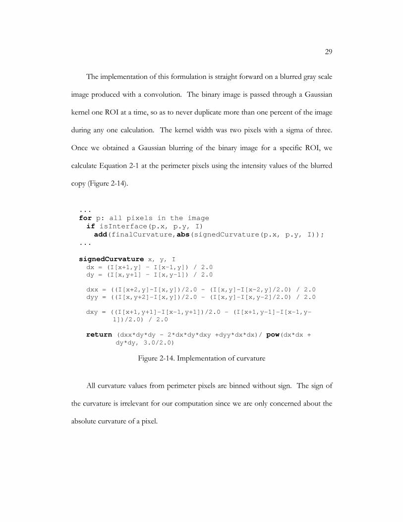
The implementation of this formulation is straight forward on a blurred gray scale

image produced with a convolution. The binary image is passed through a Gaussian

kernel one ROI at a time, so as to never duplicate more than one percent of the image

during any one calculation. The kernel width was two pixels with a sigma of three.

Once we obtained a Gaussian blurring of the binary image for a specific ROI, we

calculate Equation 2-1 at the perimeter pixels using the intensity values of the blurred

copy (Figure 2-14).

... for p: all pixels in the image if isInterface(p.x, p.y, I) add(finalCurvature, abs(signedCurvature(p.x, p.y, I));

... signedCurvature x, y, I

dx = (I[x+1,y] – I[x-1,y]) / 2.0 dy = (I[x,y+1] – I[x,y-1]) / 2.0 dxx = ((I[x+2,y]-I[x,y])/2.0 – (I[x,y]-I[x-2,y]/2. 0) / 2.0 dyy = ((I[x,y+2]-I[x,y])/2.0 – (I[x,y]-I[x,y-2]/2. 0) / 2.0 dxy = ((I[x+1,y+1]-I[x-1,y+1])/2.0 - (I[x+1,y-1]-I[ x-1,y-

1])/2.0) / 2.0 return (dxx*dy*dy - 2*dx*dy*dxy +dyy*dx*dx)/ pow(dx*dx +

dy*dy, 3.0/2.0)

Figure 2-14. Implementation of curvature

All curvature values from perimeter pixels are binned without sign. The sign of

the curvature is irrelevant for our computation since we are only concerned about the

absolute curvature of a pixel.

30

Figure 2-15. Conceptual definition of aspect ratio

2.2.7 Aspect Ratio

Aspect ratio is a metric that evaluates the overall shape and dimensions of an

object. It divides the object’s shortest span by its longest span. The concept can be

visualized by tightly fitting of a rectangle around an object and dividing the shortest

edge by the longest edge (Figure 2-15). This measure is applied to all regions of

interest individually.

Aspect ratio is one of the two metrics that depends on eigen systems. Aspect

ratio is the ratio between the length of the major and minor axis of an object. It is

inherently independent of directions, as it builds its own reference coordinate system.

The mathematical reason behind using such a system is that each region of interest

31

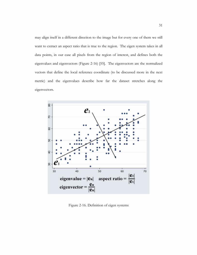
may align itself in a different direction to the image but for every one of them we still

want to extract an aspect ratio that is true to the region. The eigen system takes in all

data points, in our case all pixels from the region of interest, and defines both the

eigenvalues and eigenvectors (Figure 2-16) [55]. The eigenvectors are the normalized

vectors that define the local reference coordinate (to be discussed more in the next

metric) and the eigenvalues describe how far the dataset stretches along the

eigenvectors.

Figure 2-16. Definition of eigen systems

32

In building the eigen system we must first build a covariance matrix before we

can extract the eigenvalues and eigenvectors [8]. The covariance matrix is a matrix that

defines the variance within a set of random elements [15]. In our case our random

elements are the pixels in each region of interest. The variance within our system is

the distance between each pixel and the centroid, center of mass, in a ROI. The

covariance matrix that we can construct will be the overall covariance of a ROI

(Equation 2-2).

2

2

yxy

xyx

Equation 2-2 Definition of covariant matrix in terms of a ROI’s pixels’ x and y

coordinate

After the covariance matrix is generated the eigenvalues and eigenvectors must be

extracted from it. The technique used is the real symmetric QR algorithm described

by Golub and van Loan [21]. The eigenvalues and eigenvectors are then sorted by

eigenvalues to distinguish between the major and minor axis. The final computation is

produced by dividing the eigenvalue of the minor axis (the one with the smaller value)

by the eigenvalue of the major axis (the one with the greater value). We divide the

minor axis by the major axis (as opposed to major by minor) to produce consistent

results in the range of 0.0 and 1.0 for the final value. The final aspect ratios for each

ROI are then binned.

33

2.2.8 Eigenvector

The eigenvector metric is related to the aspect ratio metric in that it may make use

of the other half of the eigen decomposition (Figure 2-16). This metric measures the

distribution of shape alignments within an image. It takes each ROI and measures the

angle between (cosine of the angle to be exact) the ROI’s direction and the average

direction of all regions within an image. The biological reason behind this is that this

analysis is what many pathologists use behind the scenes. From my interview with

John Tomaszewski (a pathologist at the University of Pennsylvania) I discovered that

the Gleason indexing system for prostate cancer is almost completely based off of the

measurement of structural entropy within a given section. The more randomness

exists within a section the higher the grade. He also claimed that this measure helps

distinguish between cases in many other specimens as well. So inspired by this

concept we have devised a metric that attempts to capture this aspect of histology.

The implementation of this metric first determines the average the major axis of

all the ROI in an image. The major axis of the ROI is the eigenvector associated with

the greatest eigenvalue of the ROI. After obtaining the average major axis of all the

ROI it then calculates the dot product of all the ROI major axes with the average

major axis. The dot product is the representation of the cosine of the angle between

the average major axis and the major axis of each region to be binned [55]. The

34

resulting dot product is then binned into the histogram after having 1.0 added to it (to

keep the values positive since it ranges from -1.0 to 1.0).

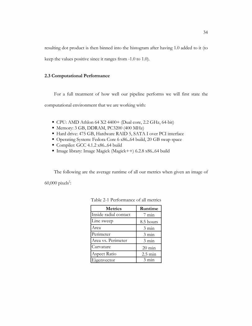
2.3 Computational Performance

For a full treatment of how well our pipeline performs we will first state the

computational environment that we are working with:

� CPU: AMD Athlon 64 X2 4400+ (Dual core, 2.2 GHz, 64-bit) � Memory: 3 GB, DDRAM, PC3200 (400 MHz) � Hard drive: 475 GB, Hardware RAID 5, SATA I over PCI interface � Operating System: Fedora Core 6 x86_64 build, 20 GB swap space � Compiler: GCC 4.1.2 x86_64 build � Image library: Image Magick (Magick++) 6.2.8 x86_64 build

The following are the average runtime of all our metrics when given an image of

60,000 pixels2:

Table 2-1 Performance of all metrics

Metrics Runtime

Inside radial contact 7 min

Line sweep 8.5 hoursArea 3 min

Perimeter 3 minArea vs. Perimeter 3 min

Curvature 20 minAspect Ratio 2.5 minEigenvector 3 min

35

It should be noted that, computationally, the distance transform is the bottleneck

of both inside radial contact and the curvature metric. The time taken by the curvature

metric is much greater than that of the inside radial contact due to the “lazy” approach

taken by the inside radial contact. The inside radial contact metric only completed a

distance transform for the inside pixels only, whereas curvature has to do both.

Aspect ratio and eigenvector metrics are both bottlenecked on the eigen

decomposition of the covariant matrix. Line sweep takes the time indicated to run on

our system primarily due to the number of cache misses that force the system to over-

utilize the north-bridge of the system bus.

2.4 Distribution analysis

After the shape distributions were generated they were processed by a variety of

analysis to determine the usability of the measures as well as the overall performance

of our pipeline. The analysis process involved both manual and automatic schemes as

we considered all outcomes.

The first step involved was post-processing the histograms to insure that the data

are not sparse or noisy. This will be described in more detail in section 3.2. After the

post processing we viewed all the histograms in the form of a graph. The graphs were

laid out in a form that has the bins on the X axis and the counts in each bin as the Y

axis. Each histogram starts at the first non-zero bin. We also looked at the graphs of

all cases laid out together to determine if any trends were evident. Overall we found

36

Grade 2: Inside radial contact

0

1

2

3

4

5

6

7

1 2 3 4 5 6 7 8 9 10 11 12 13 14 15 16 17 18 19 20 21

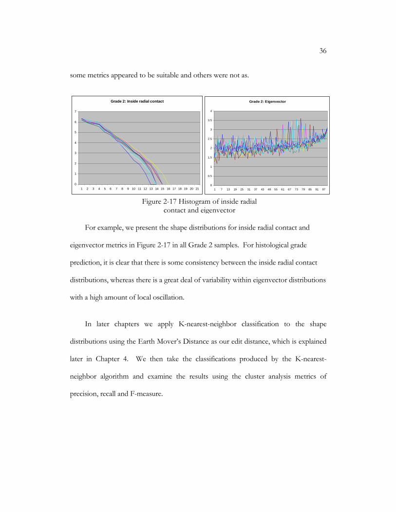
Figure 2-17 Histogram of inside radial contact and eigenvector

some metrics appeared to be suitable and others were not as.

For example, we present the shape distributions for inside radial contact and

eigenvector metrics in Figure 2-17 in all Grade 2 samples. For histological grade

prediction, it is clear that there is some consistency between the inside radial contact

distributions, whereas there is a great deal of variability within eigenvector distributions

with a high amount of local oscillation.

In later chapters we apply K-nearest-neighbor classification to the shape

distributions using the Earth Mover’s Distance as our edit distance, which is explained

later in Chapter 4. We then take the classifications produced by the K-nearest-

neighbor algorithm and examine the results using the cluster analysis metrics of

precision, recall and F-measure.

Grade 2: Eigenvector

0

0.5

1

1.5

2

2.5

3

3.5

4

1 7 13 19 25 31 37 43 49 55 61 67 73 79 85 91 97

37

C h a p t e r 3

DATA PROCESSING

The data entering the computational pipeline begin as binary segmentations of

the histological slide images and are then transformed into shape distributions,

represented as histograms, that capture the structure of the entire image in a series of

numbers that can be viewed as a signature of the image. These histograms are a

description of how often a certain value occurs when a certain geometric metric is

applied to the image. Based on how certain metrics perform, not all pixels in the

binary segmentations are desirable as well as not all numbers generated by each

measure are needed for or relevant to the final decision making process. Besides the

undesirable results of the immediate input there may also be undesirable results that

are attributed to processing much earlier in the whole process. This chapter will

address and talk about all these concerns of the computational pipeline.

3.1 Preprocessing

During the segmentation process there is a possibility of capturing some regions

that are truly regions of interest. This may happen for a variety of reasons due to the

fact that segmentation is an optimization process. Utilizing the traditional

segmentation metric, the Mumford-Shah framework [39] for measuring the

performance of a specific segmentation, there are three functionals that measure the

38

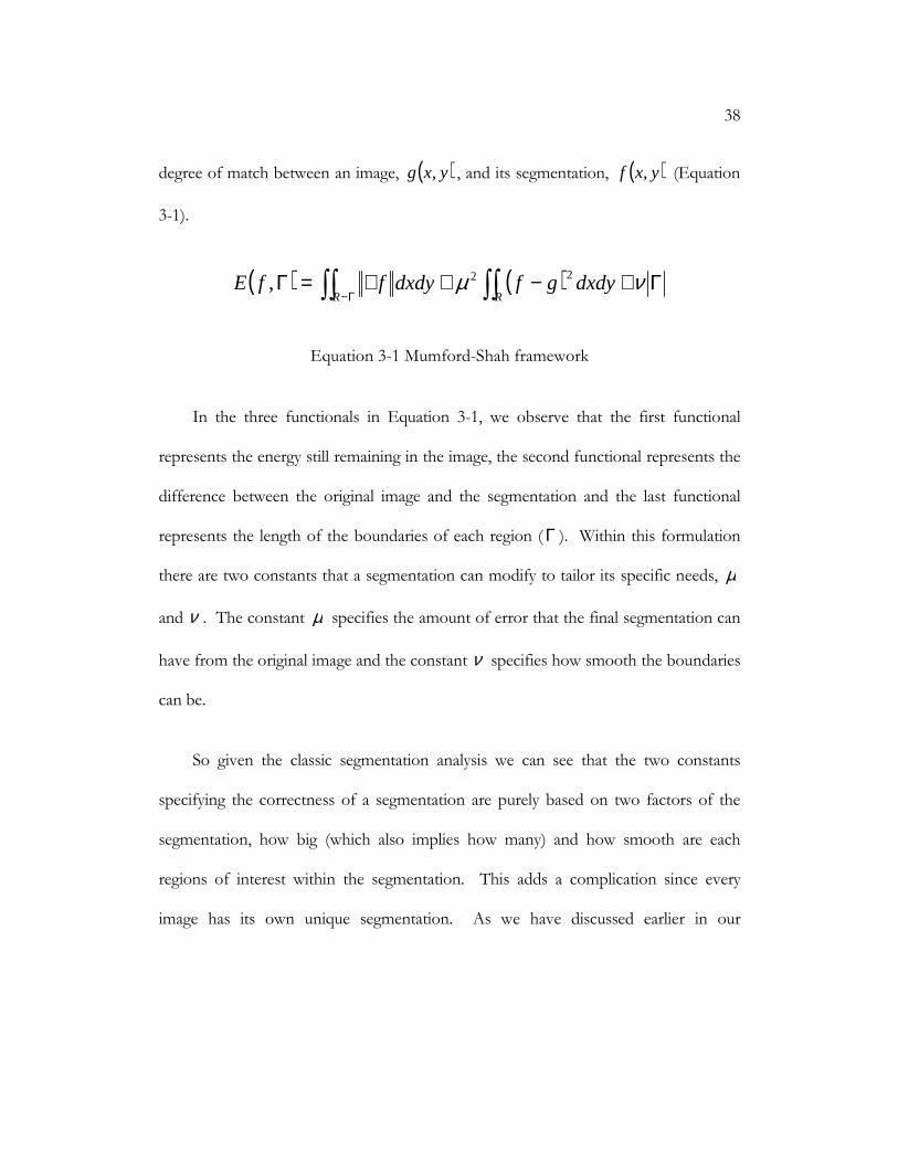
degree of match between an image, ( )yxg , , and its segmentation, ( )yxf , (Equation

3-1).

( ) ( ) Γ+−+∇=Γ ∫∫∫∫ Γ−νµ

RRdxdygfdxdyffE 22,

Equation 3-1 Mumford-Shah framework

In the three functionals in Equation 3-1, we observe that the first functional

represents the energy still remaining in the image, the second functional represents the

difference between the original image and the segmentation and the last functional

represents the length of the boundaries of each region (Γ ). Within this formulation

there are two constants that a segmentation can modify to tailor its specific needs, µ

and ν . The constant µ specifies the amount of error that the final segmentation can

have from the original image and the constant ν specifies how smooth the boundaries

can be.

So given the classic segmentation analysis we can see that the two constants

specifying the correctness of a segmentation are purely based on two factors of the

segmentation, how big (which also implies how many) and how smooth are each

regions of interest within the segmentation. This adds a complication since every

image has its own unique segmentation. As we have discussed earlier in our

39

computational framework, we depend on the accuracy and precision of those two

properties for each region of interest.

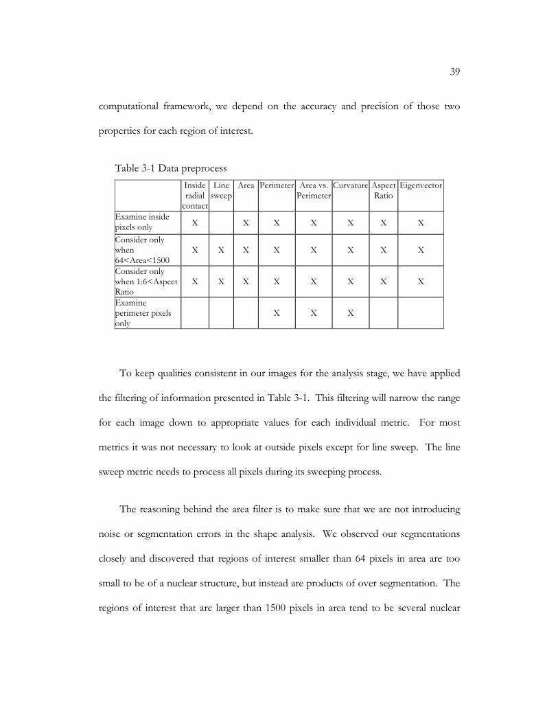
Table 3-1 Data preprocess

Inside radial contact

Line sweep

Area Perimeter Area vs. Perimeter

Curvature Aspect Ratio

Eigenvector

Examine inside pixels only X X X X X X X

Consider only when 64<Area<1500

X X X X X X X X

Consider only when 1:6<Aspect Ratio

X X X X X X X X

Examine perimeter pixels only

X X X

To keep qualities consistent in our images for the analysis stage, we have applied

the filtering of information presented in Table 3-1. This filtering will narrow the range

for each image down to appropriate values for each individual metric. For most

metrics it was not necessary to look at outside pixels except for line sweep. The line

sweep metric needs to process all pixels during its sweeping process.

The reasoning behind the area filter is to make sure that we are not introducing

noise or segmentation errors in the shape analysis. We observed our segmentations

closely and discovered that regions of interest smaller than 64 pixels in area are too

small to be of a nuclear structure, but instead are products of over segmentation. The

regions of interest that are larger than 1500 pixels in area tend to be several nuclear

40

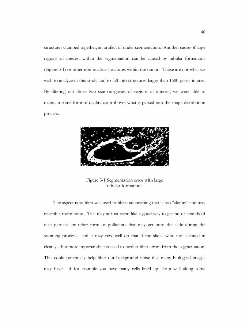
structures clumped together, an artifact of under segmentation. Another cause of large

regions of interest within the segmentation can be caused by tubular formations

(Figure 3-1) or other non-nuclear structures within the tumor. Those are not what we

wish to analyze in this study and to fall into structures larger than 1500 pixels in area.

By filtering out those two size categories of regions of interest, we were able to

maintain some form of quality control over what is passed into the shape distribution

process.

Figure 3-1 Segmentation error with large tubular formations

The aspect ratio filter was used to filter out anything that is too “skinny” and may

resemble more noise. This may at first seem like a good way to get rid of strands of

dust particles or other form of pollutants that may get onto the slide during the

scanning process... and it may very well do that if the slides were not scanned in

cleanly... but more importantly it is used to further filter errors from the segmentation.

This could potentially help filter out background noise that many biological images

may have. If for example you have many cells lined up like a wall along some

41

membrane and you were trying to segment the image. If the background is a similar

color to the nucleus structure, the segmentation process would not necessarily pick

that up as a region of interest. This filter would essentially eliminate those “mistakes”

from the segmentation.

The perimeter filter is for optimization purposes. It is used so that all metrics that

perform a computation at a perimeter pixel do not waste computation on unnecessary

pixels. The only two metrics this would affect is the area vs. perimeter and the

curvature metric.

Table 3-2 Histogram binning multipliers

Multiplier

Inside radial contact 1x

Line sweep 1x Area 0.10x Perimeter 1x Area vs. Perimeter

10x

Curvature 50x Aspect Ratio 100x Eigenvector 50x

3.2 Post process

After we have generated all the shape distributions from the filtered

segmentations we observed that some of the results of applying the metrics didn’t fall

naturally into a significant number of integer bins. To increase precision we then

42

multiplied all metric results, to increase the number of bins needed to represent the

data. We decided that a reasonable bin count was between 100 and 350, with the

exception of inside radial contact (which had a count of up to 21). This was done so

that details would not be lost and to ensure that all shape distributions had

approximately the same bin count. This is especially important in metrics where we

always divide a smaller number by a larger one, e.g. aspect ratio. The range of outputs

for those will always be from 0.0 to 1.0. It must be multiplied by a larger number to

keep everything from binning to 0. So to deal with that problem we have applied

multipliers to the results produced by applying the metrics in order to properly scale

the range of the metrics’ output (Table 3-2).

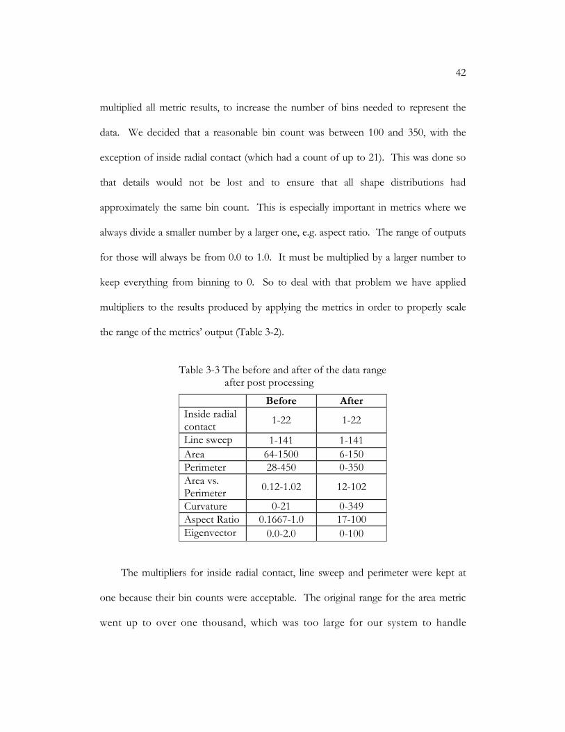
Table 3-3 The before and after of the data range after post processing

Before After

Inside radial contact

1-22 1-22

Line sweep 1-141 1-141

Area 64-1500 6-150 Perimeter 28-450 0-350 Area vs. Perimeter

0.12-1.02 12-102

Curvature 0-21 0-349 Aspect Ratio 0.1667-1.0 17-100 Eigenvector 0.0-2.0 0-100

The multipliers for inside radial contact, line sweep and perimeter were kept at

one because their bin counts were acceptable. The original range for the area metric

went up to over one thousand, which was too large for our system to handle

43

computationally using the Earth Mover’s Distance (details in chapter 4), and had to be

scaled down to allow for a more manageable size. Everything else had to be expanded

due to their extremely small original range. After the expansion, we had to do a

preliminary cutoff in the higher ranges for curvature and perimeter due to the obvious

sparseness of the data after a certain value where there are large gaps between values

that lead to only small bucket sizes. Aspect ratio had to be scaled by 100 due to the

fact that it originally ranges from 0.0 to 1.0. Eigenvector had to be scaled by fifty due

to the fact that it ranges from 0.0 to 2.0 from the linear shift of 1.0. Aspect ratio

originally ranges from 0.0 to 1.0 because at best, it can be square, where the ratio is 1:1

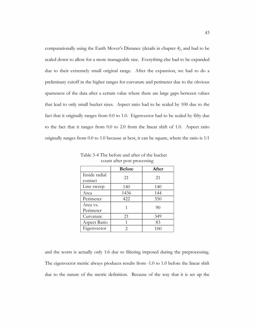
Table 3-4 The before and after of the bucket count after post processing

Before After

Inside radial contact

21 21

Line sweep 140 140

Area 1436 144 Perimeter 422 350 Area vs. Perimeter

1 90

Curvature 21 349 Aspect Ratio 1 83 Eigenvector 2 100

and the worst is actually only 1:6 due to filtering imposed during the preprocessing.

The eigenvector metric always produces results from -1.0 to 1.0 before the linear shift

due to the nature of the metric definition. Because of the way that it is set up the

44

eigenvectors can only range between 0 and 180 degrees from the average direction.

The reason is that if it is more than 180 degrees or less than 0 degrees of the major axis

it would become redundant since the definition of an eigen system defines that the

eigenvectors that forms it is the orthonormal basis of the vector space [55]. The value

of cosine(0) in degrees is 1.0 and cosine(180) in degrees is -1.0. The ranges of values

produced by each metric before and after scaling are presented in Table 3-4. The

bucket counts produced by each metric before and after scaling are presented in Table

3-4.

We discovered that logarithmic scale is better than a linear one to one mapping of

the values within each bucket. One of the initial reasons for doing this is that

everything in natures seems to be either in an exponential scale or logarithmic scale.

Take for example sound decay (exponential) and population growth (exponential). We

also discovered that a variety of image analysis texts also suggests a logarithmic scale

over linear one to one scale [11] [58] [22] [17]. After observing our data, we did see an

exponential growth in value in most cases.

The other question we considered was do we need analyze all bins in each

histogram? The histograms are very good in that they describe the structures in the

entire image completely according to one metric, but are all the information contained

in them significant? Depending on the shape distribution we are working with, we

argue that some of its bins may be discarded. In certain cases we argue that using all

45

bins will add significant noise/randomness into the analysis, and this makes the

analysis meaningless. So to increase the significance of and to minimize noise, and

therefore improve the predictability of the data, we propose to crop the shape

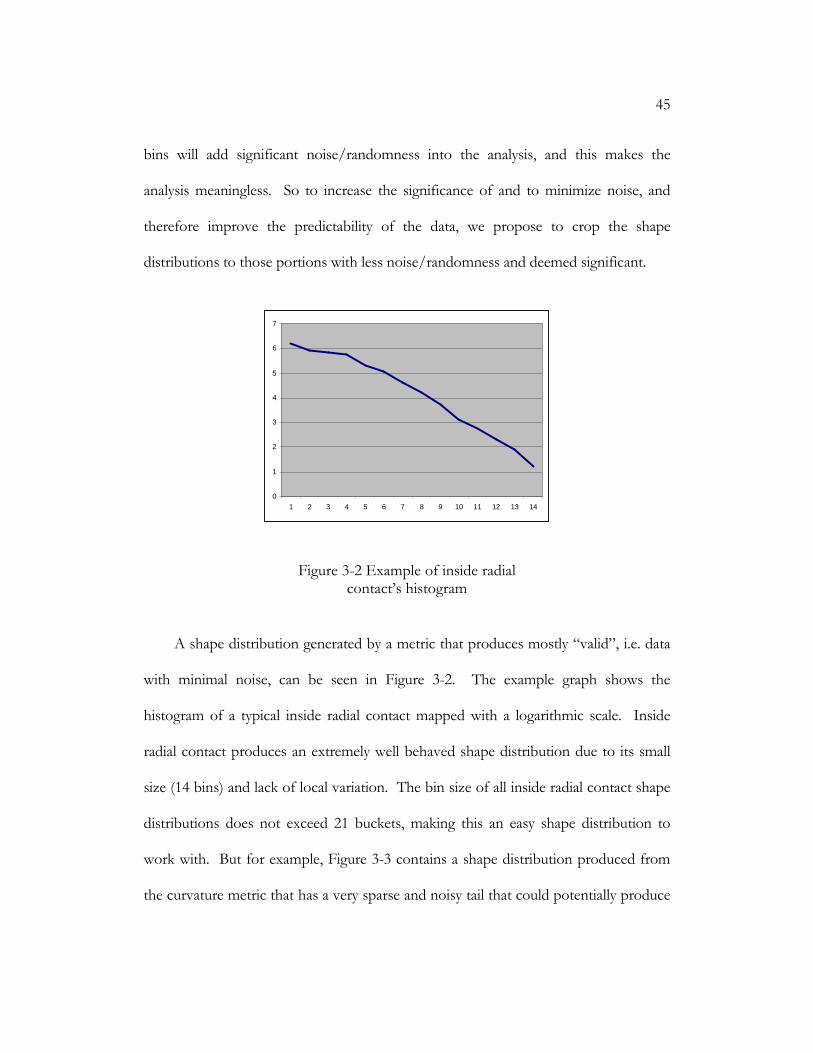
distributions to those portions with less noise/randomness and deemed significant.

0

1

2

3

4

5

6

7

1 2 3 4 5 6 7 8 9 10 11 12 13 14

Figure 3-2 Example of inside radial contact’s histogram

A shape distribution generated by a metric that produces mostly “valid”, i.e. data

with minimal noise, can be seen in Figure 3-2. The example graph shows the

histogram of a typical inside radial contact mapped with a logarithmic scale. Inside

radial contact produces an extremely well behaved shape distribution due to its small

size (14 bins) and lack of local variation. The bin size of all inside radial contact shape

distributions does not exceed 21 buckets, making this an easy shape distribution to

work with. But for example, Figure 3-3 contains a shape distribution produced from

the curvature metric that has a very sparse and noisy tail that could potentially produce

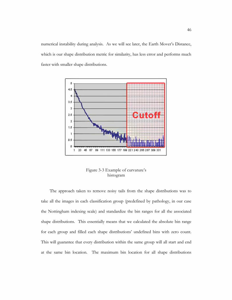
46

numerical instability during analysis. As we will see later, the Earth Mover’s Distance,

which is our shape distribution metric for similarity, has less error and performs much

faster with smaller shape distributions.

Figure 3-3 Example of curvature’s histogram

The approach taken to remove noisy tails from the shape distributions was to

take all the images in each classification group (predefined by pathology, in our case

the Nottingham indexing scale) and standardize the bin ranges for all the associated

shape distributions. This essentially means that we calculated the absolute bin range

for each group and filled each shape distributions’ undefined bins with zero count.

This will guarantee that every distribution within the same group will all start and end

at the same bin location. The maximum bin location for all shape distributions

47

produced by a particular metric is defined to be the maximum of all the first zero bin

locations. This effectively removes the “noisy tails” from the shape distributions. If

the shape distributions have zero bins preceding any significant portions then the

minimum bin will be defined by the minimum zero bin of all the zero bins preceding

the data. By doing this we will ensure that all processed shape distributions have noise

removed from their fronts and tails. The only problem that this could cause would be

an abnormal cutoff for shape distributions with a zero bucket in the middle.

Fortunately for our data, this did not occur.

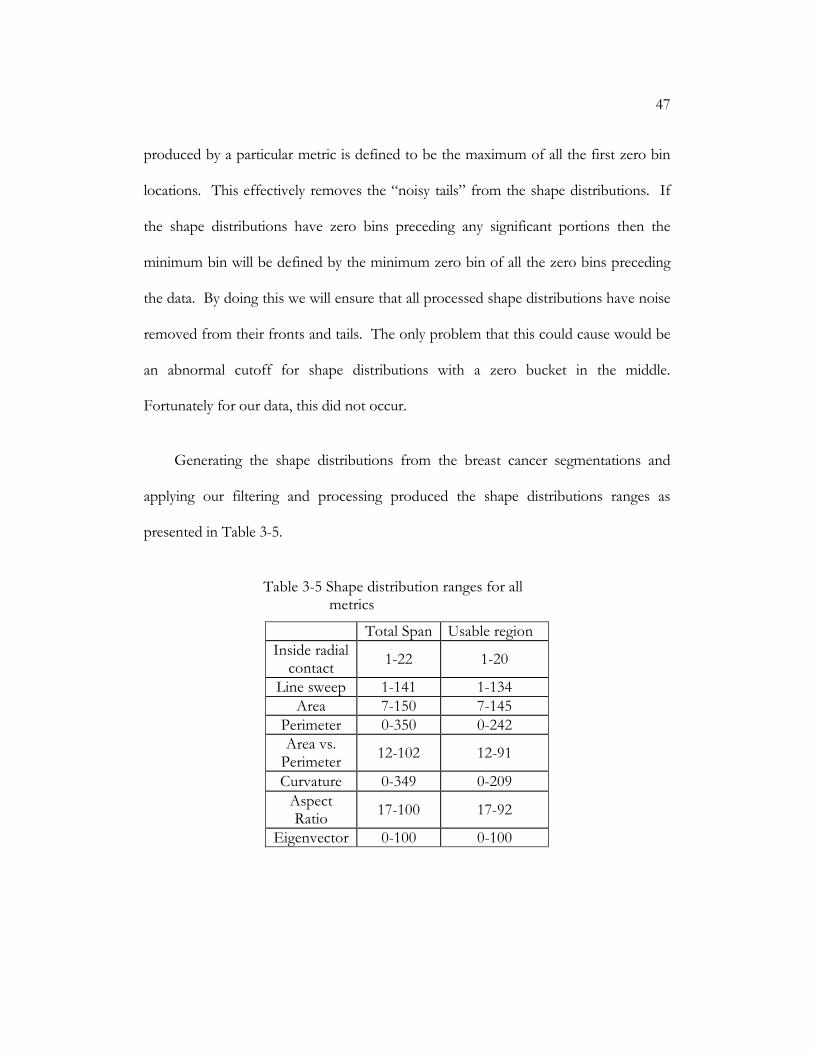
Generating the shape distributions from the breast cancer segmentations and

applying our filtering and processing produced the shape distributions ranges as

presented in Table 3-5.

Table 3-5 Shape distribution ranges for all metrics

Total Span Usable region Inside radial contact

1-22 1-20

Line sweep 1-141 1-134 Area 7-150 7-145

Perimeter 0-350 0-242 Area vs. Perimeter

12-102 12-91

Curvature 0-349 0-209

Aspect Ratio

17-100 17-92

Eigenvector 0-100 0-100

48

3.3 Pre-segmentation dependencies

The last issue regarding data that needs to be mentioned are potential problems

produced by the pre-segmentation phase of the pipeline. Errors from this phase may

have been propagated from the segmentation phase and could have skewed the

distributions of our shape distributions and, ultimately, the predictive power of the

final stage.

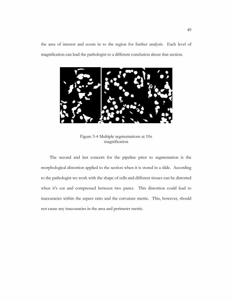
The first problem that we noticed throughout our work was that the level of

magnification used during the scanning stage of the pipeline might skew the results of

our metrics. We see the ill effects of magnification mostly in the curvature metric

where a majority of the shape distributions exhibit sparse, noisy tails. Examining the

segmentation in Figure 3-4 it can be seen that very little of the roughness in most

structures is captured. In fact only the major turns on the contour of each region is

captured. It is clear to see that this kind of segmentation can not differentiate very

much between two histological images.

Despite of the error that this causes in the curvature metric, this could be the

perfect magnification for other metrics. So we do feel that it might be good idea to

consider multiple levels of magnification when analyzing histology segmentations. We

need to discover the optimal level of magnification for each metric to increase the

predictability of each metric. This is also the procedure used by a pathologist when

examining a section. He/she will first view the slide at a low magnification, identify

49

the area of interest and zoom in to the region for further analysis. Each level of

magnification can lead the pathologist to a different conclusion about that section.

Figure 3-4 Multiple segmentations at 10x magnification

The second and last concern for the pipeline prior to segmentation is the

morphological distortion applied to the section when it is stored in a slide. According

to the pathologist we work with the shape of cells and different tissues can be distorted

when it’s cut and compressed between two panes. This distortion could lead to

inaccuracies within the aspect ratio and the curvature metric. This, however, should

not cause any inaccuracies in the area and perimeter metric.

50

C h a p t e r 4

ANALYSIS

Once the shape distributions are generated, they are analyze to determine how

effectively each metric correlates an image to its histological grade. We have devised a

few methods for analyzing the histograms that represent the shape distributions. The

key to quantifying the effectiveness of a metric is to determine if it can correctly

identify the classification of a sample of a known grade.

In our first approach we attempted to classify clusters of shape distribution in a

high dimensional space. We treated every case as a point in a high dimensional space

and attempted to find clusters of classification groups using a L-2 norm. This led us to

unpromising data that does not seem to cluster well.

The second approach we took was to try to determine the classification of a case

based on querying our known cases using K-nearest-neighbor. We attempted to

perform such an analysis on the whole histogram that represents the shape distribution

and validated it against standard metrics used in information retrieval (precision, recall

and F-measure [48]). By performing the validations we discovered that by comparing

windows of sub-regions within the histograms instead of the whole histogram we

would be able to achieve better performance with each geometric metric.

51

After performing the validation on all analysis of the sub-regions we were able to

determine certain criteria that would potentially gain the best performance with our

given data set for each geometric metrics. Due to the size of our data we were able to

only make suggestive claims as to how well each of our geometric measures performed

in our given scenario. All this and more will be described in this chapter.

4.1 Earth mover’s distance

The Earth Mover’s Distance (EMD) is an algorithm devised in Stanford in the

late 90s for distribution analysis [51]. The purpose of EMD is to compare two

histograms and purpose a measure of the similarity between the two using an

optimization algorithm. Similarity, defined by EMD, is the minimal energy needed to

transform one distribution into another. It can be described using the analogy of

trying to fill a set of holes by moving dirt from a mound of dirt. We have chosen

EMD over other algorithms primarily due to the success that was attributed to it in the

computer vision domain [50].

The reason that we chose to use EMD over all other measures was because it was

considered the optimal algorithm for comparing two histograms. One of the primary

reasons why EMD is better for our purpose is due to EMD’s capability to compare

between two histograms of varying lengths. EMD has a nice property of treating all

vectors given to it as distributions, where size differences do not cause computational

problems as do most histogram based algorithms [51].

52

After using EMD for awhile we also noticed a few properties of it that are worth

noting. One of them relates to the previously stated property that we have observed.

When given two distributions of varying length EMD will treat them as if they are the

same length starting at the same bin location. What that means is that if you have one

histogram starting at n and another starting at n+m, EMD will treat the histogram as if

both started at the same location. That is a problem if we are comparing regions. Due

to the displacement and potential scaling, padding in zeros in the front and back of a

histogram to normalize the length will cause the EMD to produce a different result

when compared to unpadded comparisons.

Another issue with EMD is that due to the arbitrary offset and length it creates

for two histograms it will view each bin as a percent of the total mass. The sum of all

bin values will sum to one. This is a good property for histograms of small values but

will get numerically unstable as the histogram bin count increases. This is also a

problem if the total sum of all values is large as well. We have tackled this problem by

converting all histograms to log scale. A problem with log scale is that there is also a

potential for sparse data to create numerical instability as well. A sparse histogram will

cause the algorithm to require a higher EPSILON to converge, which causes potential

for more error in the final result.

The last issue with EMD that is worth mentioning is that it is not linearly additive.

What that means is if you take histogram H1 and histogram H2 and you do an EMD

53

calculation on it, it will come up with result A. But if you break up H1 and H2 to be

four halves instead of two wholes, the sum of EMD(FirstHalf(H1), FirstHalf (H2) +

EMD(SecondHalf(H1, SecondHalf (H2)) will not equal EMD(H1, H2). The reason

behind this is the fact that EMD is an optimization problem and therefore does not

grow linearly. Therefore there is no simple means to breakdown the histograms and

compute it by parts. This is important in that the EMD calculation will be directly

constrained by the size of the problem. Though this problem shouldn’t really be an

issue due to the size of most problems, it can nevertheless be handled by either scaling

or trimming ends of the histograms if the size of the problem really calls for it.

4.2 Shape distribution sub-regions

The one consideration that needs to be taken into account is sub-regions within

each distribution. As discussed in data post processing, we hinted at the fact that

maybe the entire histogram would not be needed for prediction and matching. As we

proceeded with our experimentations we discovered that we only need certain sub-

regions of a histogram to produce acceptable comparison results, even after filtering

out the sparse regions (as explained in data post processing).

One of the key ideas behind finding a good sub-region for comparison is to find a

region of good separation between classification groups. A visual inspection, as shown

in Figure 4-1, shows that it is clear that certain sub-regions are better separated than

others. The sub-region does not necessarily have to separate all classification groups in

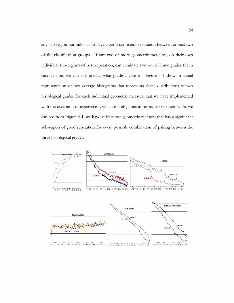
54

any sub-region but only has to have a good consistent separation between at least two

of the classification groups. If any two or more geometric measures, on their own

individual sub-regions of best separation, can eliminate two out of three grades that a

case can be, we can still predict what grade a case is. Figure 4-1 shows a visual

representation of two average histograms that represents shape distributions of two

histological grades for each individual geometric measure that we have implemented

with the exception of eigenvector, which is ambiguous in respect to separation. As we

can see from Figure 4-1, we have at least one geometric measure that has a significant

sub-region of good separation for every possible combination of pairing between the

three histological grades.

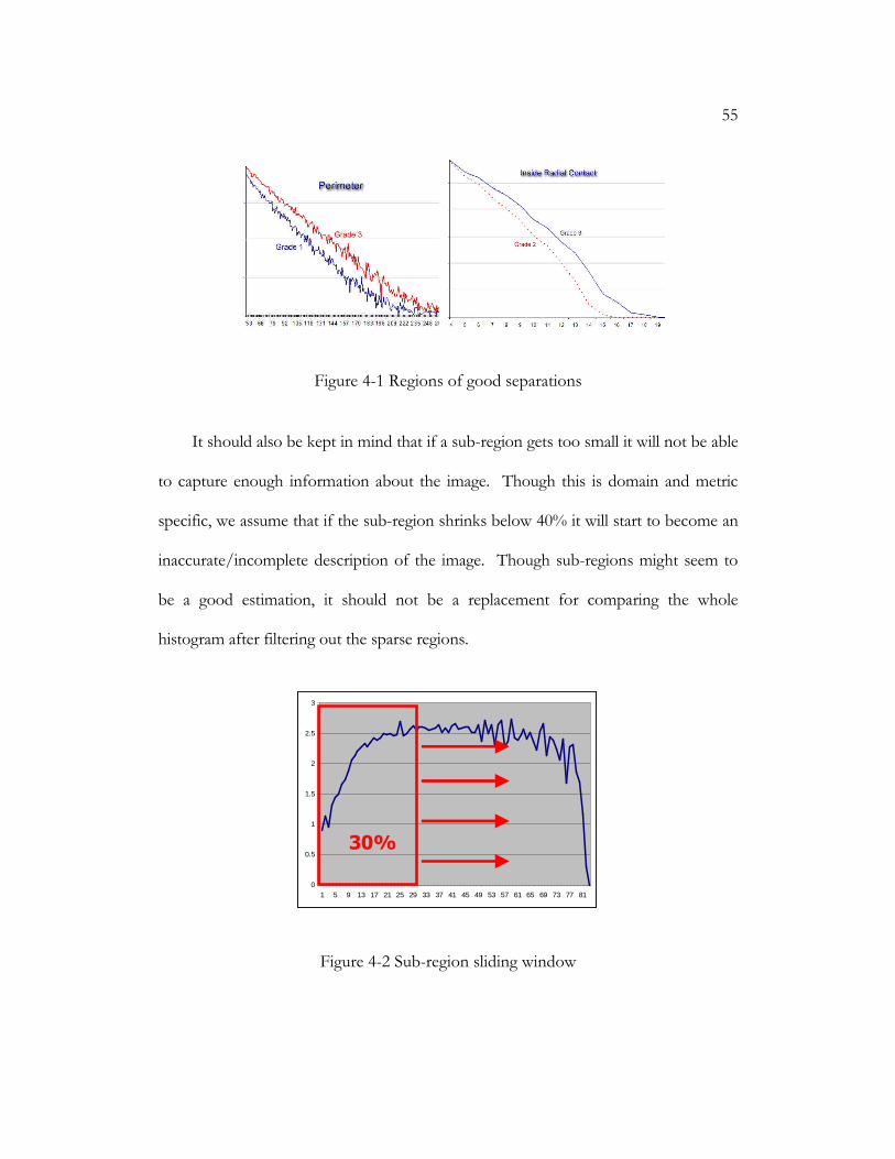
55

Figure 4-1 Regions of good separations

It should also be kept in mind that if a sub-region gets too small it will not be able

to capture enough information about the image. Though this is domain and metric

specific, we assume that if the sub-region shrinks below 40% it will start to become an

inaccurate/incomplete description of the image. Though sub-regions might seem to

be a good estimation, it should not be a replacement for comparing the whole

histogram after filtering out the sparse regions.

0

0.5

1

1.5

2

2.5

3

1 5 9 13 17 21 25 29 33 37 41 45 49 53 57 61 65 69 73 77 81

30%

0

0.5

1

1.5

2

2.5

3

1 5 9 13 17 21 25 29 33 37 41 45 49 53 57 61 65 69 73 77 81

30%

Figure 4-2 Sub-region sliding window

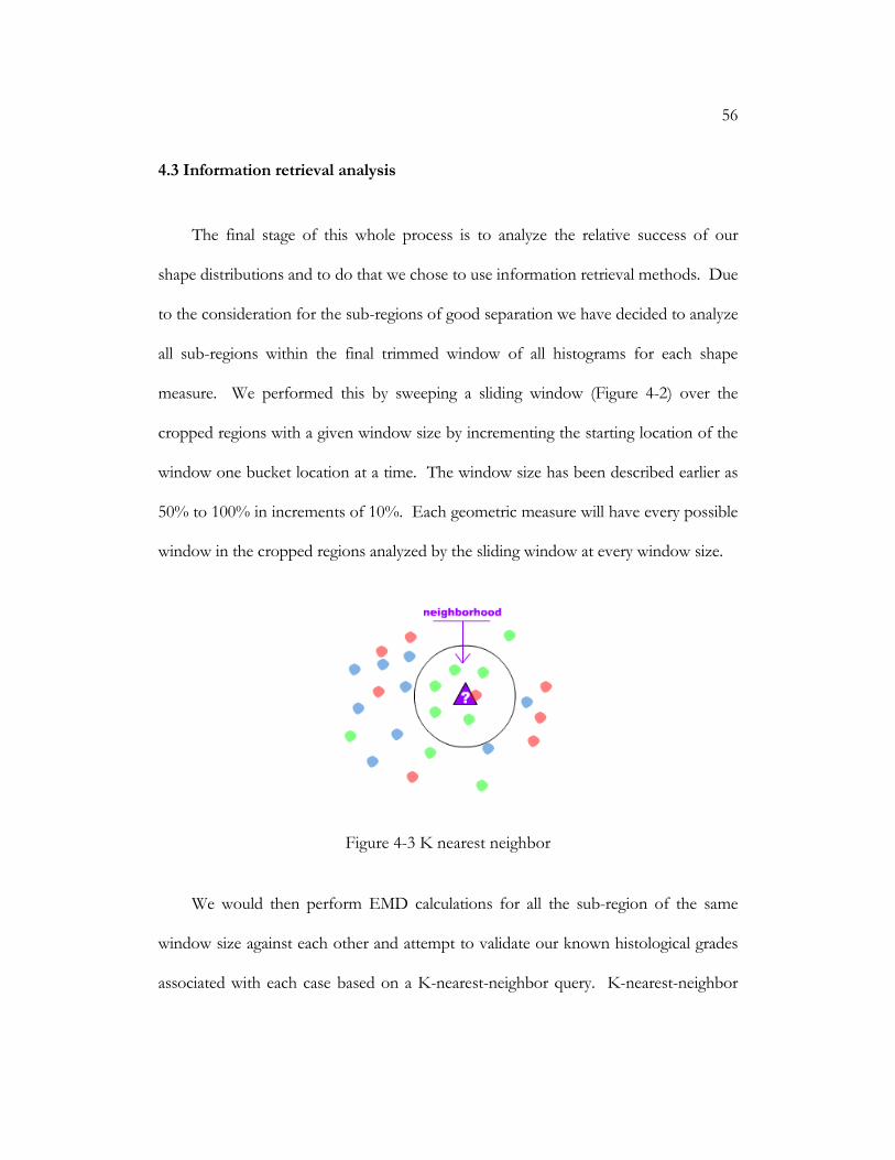
56

4.3 Information retrieval analysis

The final stage of this whole process is to analyze the relative success of our

shape distributions and to do that we chose to use information retrieval methods. Due

to the consideration for the sub-regions of good separation we have decided to analyze

all sub-regions within the final trimmed window of all histograms for each shape

measure. We performed this by sweeping a sliding window (Figure 4-2) over the

cropped regions with a given window size by incrementing the starting location of the

window one bucket location at a time. The window size has been described earlier as

50% to 100% in increments of 10%. Each geometric measure will have every possible

window in the cropped regions analyzed by the sliding window at every window size.

Figure 4-3 K nearest neighbor

We would then perform EMD calculations for all the sub-region of the same

window size against each other and attempt to validate our known histological grades

associated with each case based on a K-nearest-neighbor query. K-nearest-neighbor

57

takes a set of data points and using some form of edit distance finds the K closest

points around an unknown point (Figure 4-3). So in our case of analyzing the

performance of a given sub-regions in a given geometric measure we would, for all

cases, find the K nearest cases to a given case based on EMD distance and try to form

a result for our K-nearest-neighbor query based on a vote between all K nearest cases.

The final result of the query would be the histological grade with the highest vote [11]

[17]. If there is a tie in the vote, the given case would be classified as “unknown”.

The K values that we chose for the classification process are 4, 7, and 10. We

chose these values in order to guarantee that only a two way tie is possible if a tie

exists, eliminating the possibility of three way ties, as shown by K mod 3 producing 1

for each K value. We chose to omit the K value of 1 from our analysis because we

observe that it wouldn’t be any different from just getting the closest case, providing

an unreliable classification. We did not go above 10 for the K value because we only

have ten cases for each grade, providing us with no meaningful information.

The next step that we took was to take the queries of each sub-region of each

geometric measure formed by K nearest neighbor and analyzing them using the

metrics of precision, recall and F-measure. As a precursor, we should define the

following terms [48]:

− True Positive (TP): In a given set of cases with known classification, how many

cases were correctly classified into class X by a classifier.

58

− False Positive (FP): In the same set of cases, how many cases that don’t belong

in class X were classified into class X by the classifier.

− False Negative (FN): In the same set of cases, how many cases that belong in

class X did not make it into class X.

Precision measure how many correct queries were performed for each

histological grade in respect to all the queries that maps a case to that specific

histological grade. The precision of K nearest neighbor in histological grade jC is

generated by taking the sum of all correct queries (true positives, TP) and dividing it by

the total number of queries performed (true positives + false positives, TP + FP)

(Equation 4-1). The goal of each window is to maximize precision [48].

Precision ( )FPTP

TPC j +

=

Equation 4-1 Precision measure

The recall metric measures how many cases of a certain histological grade were

able to get mapped back to their original classification using a query. Recall is the ratio

between the correct queries for the histological grade (TP) and all the cases that belong

to the histological grade (TP + FN). The goal of each window is to maximize recall

[48].

59

Recall ( )FNTP

TPC j +

=

Equation 4-2 Recall measure

The F-measure is a metric that combines both precision and recall in a harmonic

mean (geometric mean squared over arithmetic mean) to provide an overall

performance measure that combines both individual measures (Equation 4-3). The

scale of the F-measure is from 0.0 to 1.0. Almost 0.0 is the worst performance and 1.0

is best [48] [35].

( )recallprecision

recallprecisionCF j +

××= 2

Equation 4-3 F-measure

The full process of analyzing each window will consist of computing precision,

recall and F-measure for each window. Analysis for each window will be stored and

ranked using F-measure as key. A summary of the best performance, in respect F-

measure, can be found in Appendix A. The metric for best performance is ranked

primarily by F-measure and if there is a tie with the F-measure it will be ranked

secondarily by window size second. A visualization of this data can be seen below

with Figure 4-4, Figure 4-6 and Figure 4-8 and descriptions. The full set of data for our

images acquired from this process can be found in the link in Appendix B.

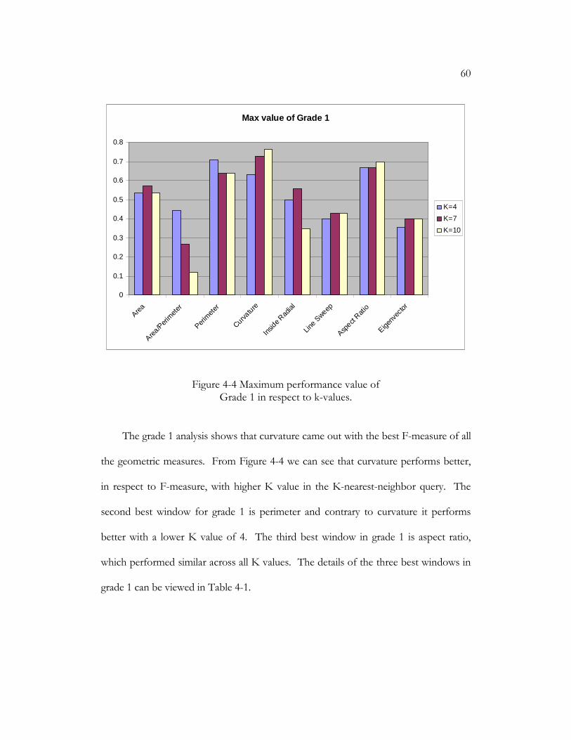
60

Max value of Grade 1

0

0.1

0.2

0.3

0.4

0.5

0.6

0.7

0.8

Area

Area/P

erim

eter

Perim

eter

Curvatu

re

Insid

e Rad

ial

Line S

weep

Aspect

Ratio

Eigenv

ector

K=4

K=7

K=10

Figure 4-4 Maximum performance value of Grade 1 in respect to k-values.

The grade 1 analysis shows that curvature came out with the best F-measure of all

the geometric measures. From Figure 4-4 we can see that curvature performs better,

in respect to F-measure, with higher K value in the K-nearest-neighbor query. The

second best window for grade 1 is perimeter and contrary to curvature it performs

better with a lower K value of 4. The third best window in grade 1 is aspect ratio,

which performed similar across all K values. The details of the three best windows in

grade 1 can be viewed in Table 4-1.

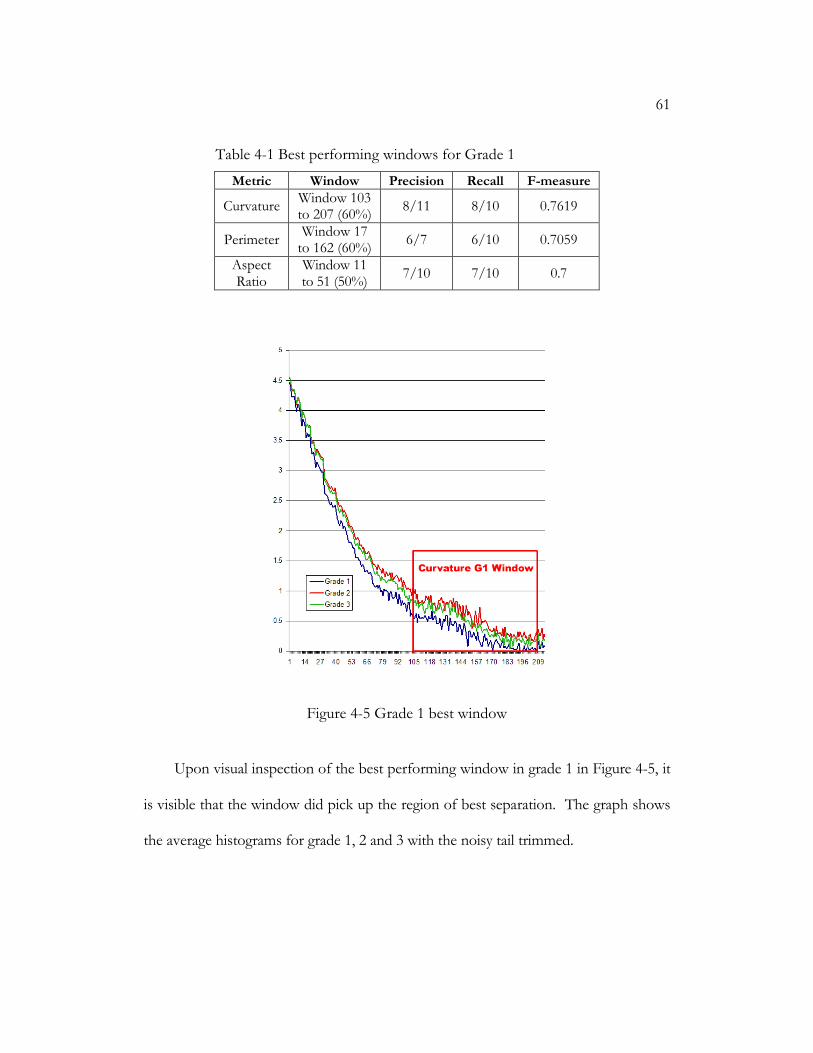
61

Table 4-1 Best performing windows for Grade 1

Metric Window Precision Recall F-measure

Curvature Window 103 to 207 (60%)

8/11 8/10 0.7619

Perimeter Window 17 to 162 (60%)

6/7 6/10 0.7059

Aspect Ratio

Window 11 to 51 (50%)

7/10 7/10 0.7

Figure 4-5 Grade 1 best window

Upon visual inspection of the best performing window in grade 1 in Figure 4-5, it

is visible that the window did pick up the region of best separation. The graph shows

the average histograms for grade 1, 2 and 3 with the noisy tail trimmed.

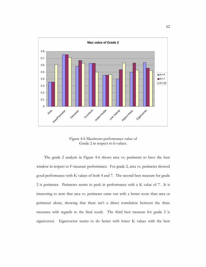
62

Max value of Grade 2

0

0.1

0.2

0.3

0.4

0.5

0.6

0.7

0.8

Area

Area/P

erim

eter

Perim

eter

Curvatu

re

Insid

e Rad

ial

Line S

weep

Aspect

Ratio

Eigenv

ector

K=4

K=7

K=10

Figure 4-6 Maximum performance value of Grade 2 in respect to k-values.

The grade 2 analysis in Figure 4-6 shows area vs. perimeter to have the best

window in respect to F-measure performance. For grade 2, area vs. perimeter showed

good performance with K values of both 4 and 7. The second best measure for grade

2 is perimeter. Perimeter seems to peek in performance with a K value of 7. It is

interesting to note that area vs. perimeter came out with a better score than area or

perimeter alone, showing that there isn’t a direct correlation between the three

measures with regards to the final result. The third best measure for grade 2 is

eigenvector. Eigenvector seems to do better with lower K values with the best

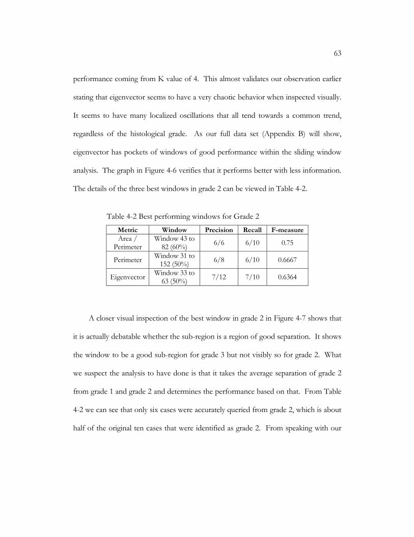
63

performance coming from K value of 4. This almost validates our observation earlier

stating that eigenvector seems to have a very chaotic behavior when inspected visually.

It seems to have many localized oscillations that all tend towards a common trend,

regardless of the histological grade. As our full data set (Appendix B) will show,

eigenvector has pockets of windows of good performance within the sliding window

analysis. The graph in Figure 4-6 verifies that it performs better with less information.

The details of the three best windows in grade 2 can be viewed in Table 4-2.

Table 4-2 Best performing windows for Grade 2

Metric Window Precision Recall F-measure

Area / Perimeter

Window 43 to 82 (60%)

6/6 6/10 0.75

Perimeter Window 31 to 152 (50%)

6/8 6/10 0.6667

Eigenvector Window 33 to

63 (50%) 7/12 7/10 0.6364

A closer visual inspection of the best window in grade 2 in Figure 4-7 shows that

it is actually debatable whether the sub-region is a region of good separation. It shows

the window to be a good sub-region for grade 3 but not visibly so for grade 2. What

we suspect the analysis to have done is that it takes the average separation of grade 2

from grade 1 and grade 2 and determines the performance based on that. From Table

4-2 we can see that only six cases were accurately queried from grade 2, which is about

half of the original ten cases that were identified as grade 2. From speaking with our

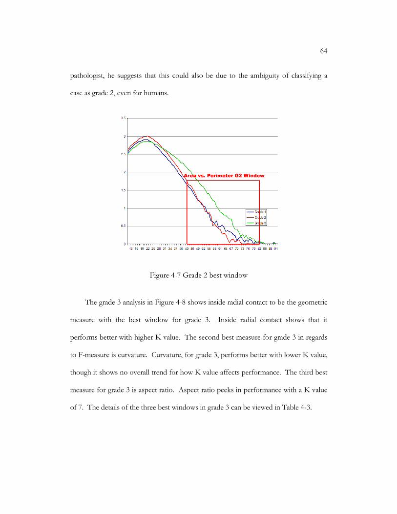
64

pathologist, he suggests that this could also be due to the ambiguity of classifying a

case as grade 2, even for humans.

Figure 4-7 Grade 2 best window

The grade 3 analysis in Figure 4-8 shows inside radial contact to be the geometric

measure with the best window for grade 3. Inside radial contact shows that it

performs better with higher K value. The second best measure for grade 3 in regards

to F-measure is curvature. Curvature, for grade 3, performs better with lower K value,

though it shows no overall trend for how K value affects performance. The third best

measure for grade 3 is aspect ratio. Aspect ratio peeks in performance with a K value

of 7. The details of the three best windows in grade 3 can be viewed in Table 4-3.

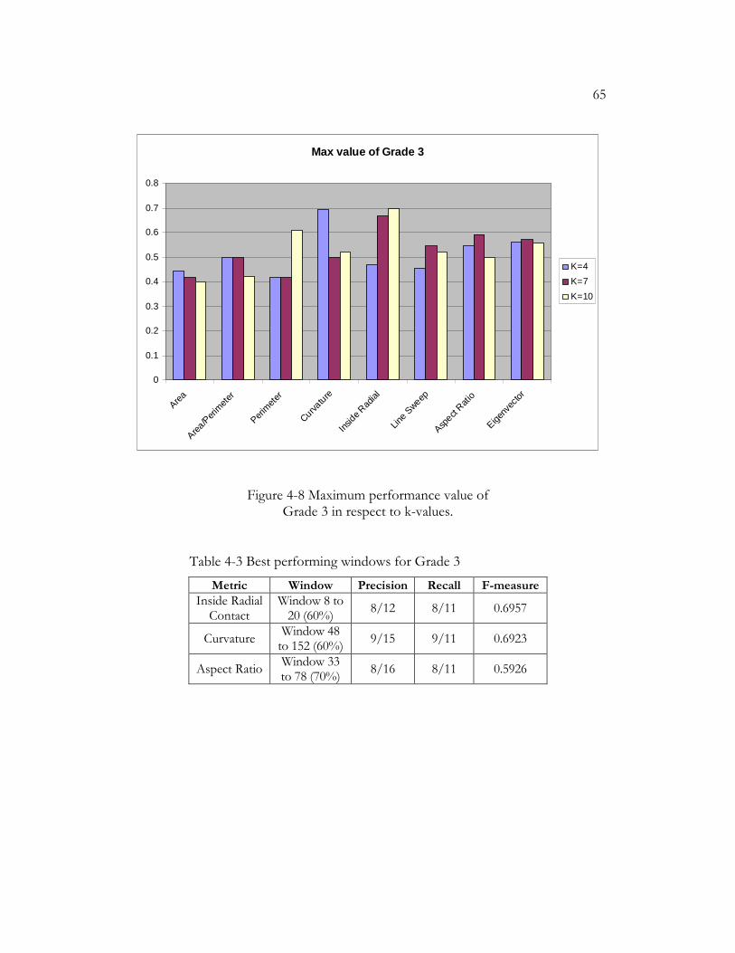
65

Max value of Grade 3

0

0.1

0.2

0.3

0.4

0.5

0.6

0.7

0.8

Area

Area/P

erim

eter

Perim

eter

Curvatu

re

Insid

e Rad

ial

Line S

weep

Aspect

Ratio

Eigenv

ector

K=4

K=7

K=10

Figure 4-8 Maximum performance value of Grade 3 in respect to k-values.

Table 4-3 Best performing windows for Grade 3

Metric Window Precision Recall F-measure

Inside Radial Contact

Window 8 to 20 (60%)

8/12 8/11 0.6957

Curvature Window 48 to 152 (60%)

9/15 9/11 0.6923

Aspect Ratio Window 33 to 78 (70%)

8/16 8/11 0.5926

66

Figure 4-9 Grade 3 best window

From visually inspecting the best performing window in grade 3 in Figure 4-9 we

can see that it is obvious that the window picked out the sub-region of best separation.

It clearly distinguishes the grade 3 average histogram from the other two grades within

the region. Though it is not as clear at the tail of the histogram, it is the best sub-

region of separation between bucket locations of 8 and 13.

67

C h a p t e r 5

CONCLUSION

5.1 Conclusion

This thesis has investigated the use of shape distributions in the analysis of

segmentations of histological images. From our studies we have discovered a way to

analyze the performance of shape distributions based on their ability to estimate

histological grade. We explored the feasibility and performance of the Earth Mover’s

Distance as an edit distance in our analysis. While our results are suggestive of

predictions using visual and quantitative methods, they are not predictive at this point.

What we have shown is a quantitative technique for determining best windows of

predictive results for each metric and K-value when using the K-nearest-neighbor

method, regardless of the techniques and edit distances used.

Besides the analysis of shape distributions for histological segmentations we were

also able to explore the extension of using a line as a shape function. Using the line

sweep shape function we were able to emulate the profile shape function [47] and take

it further by collecting all possible profiles of the image.

68

5.2 Future work

Though this approach offers good start, there is more that can be done to

improve it. One of the major improvements that could be implemented is the

incorporation of multi-level magnification. We propose to apply a Gaussian pyramid

approach to help add the ability to zoom out of the image. It would also be useful to

have images of very high magnification to start with when working with such scheme.

Many of the metrics would benefit greatly from added details in the image, as well as a

more zoomed out view.

This work can be improved if other classification techniques and edit distances

are explored. This can lead to measuring and comparing the relative quality of each

technique and edit distance in relationship to the data given. We would also like to

determine if shape distributions may be improved with other techniques and edit

distances.

Our study would have benefited from more histological segmentations for

analysis. This would provide more statistical information. More data would allow us

to move closer to a predictive capability. With enough evidence we could possibly

calculate a statistical likelihood of a certain case being a certain grade.

69

With enough data and evidence we would eventually want this work to be

validated for image archiving and cataloging purposes. This work can easily be ported

over for image archiving and cataloging and we wish fully explore this at a later time.

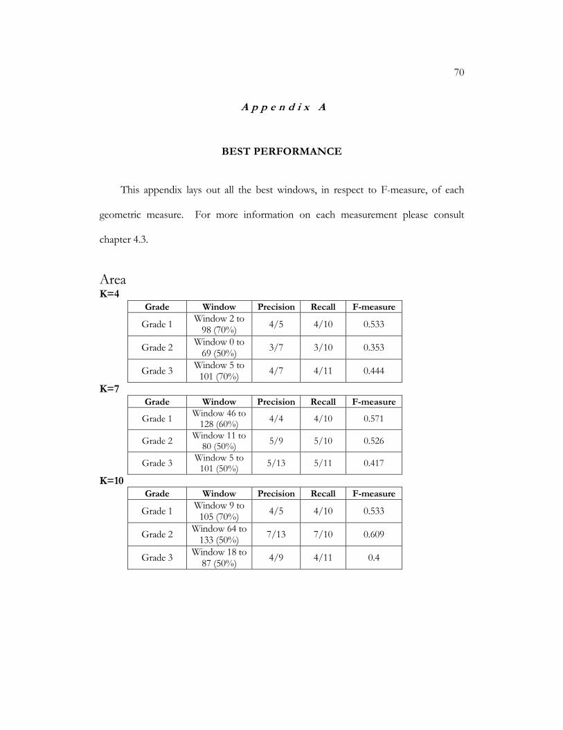
70

A p p e n d i x A

BEST PERFORMANCE

This appendix lays out all the best windows, in respect to F-measure, of each

geometric measure. For more information on each measurement please consult

chapter 4.3.

Area K=4

Grade Window Precision Recall F-measure

Grade 1 Window 2 to 98 (70%)

4/5 4/10 0.533

Grade 2 Window 0 to 69 (50%)

3/7 3/10 0.353

Grade 3 Window 5 to 101 (70%)

4/7 4/11 0.444

K=7 Grade Window Precision Recall F-measure

Grade 1 Window 46 to 128 (60%)

4/4 4/10 0.571

Grade 2 Window 11 to

80 (50%) 5/9 5/10 0.526

Grade 3 Window 5 to 101 (50%)

5/13 5/11 0.417

K=10 Grade Window Precision Recall F-measure

Grade 1 Window 9 to 105 (70%)

4/5 4/10 0.533

Grade 2 Window 64 to 133 (50%)

7/13 7/10 0.609

Grade 3 Window 18 to

87 (50%) 4/9 4/11 0.4

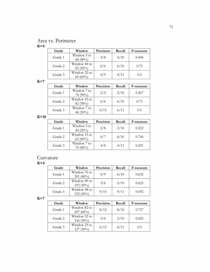
71

Area vs. Perimeter K=4

Grade Window Precision Recall F-measure

Grade 1 Window 5 to 68 (80%)

4/8 4/10 0.444

Grade 2 Window 44 to

83 (50%) 6/6 6/10 0.75

Grade 3 Window 22 to

69 (60%) 4/5 4/11 0.5

K=7 Grade Window Precision Recall F-measure

Grade 1 Window 7 to 78 (90%)

2/5 2/10 0.267

Grade 2 Window 43 to

82 (50%) 6/6 6/10 0.75

Grade 3 Window 7 to 46 (50%)

6/13 6/11 0.5

K=10 Grade Window Precision Recall F-measure

Grade 1 Window 5 to 44 (50%)

2/8 2/10 0.222

Grade 2 Window 15 to

62 (60%) 6/7 6/10 0.706

Grade 3 Window 7 to 70 (80%)

4/8 4/11 0.421

Curvature K=4

Grade Window Precision Recall F-measure

Grade 1 Window 76 to 201 (60%)

6/9 6/10 0.632

Grade 2 Window 89 to 193 (50%)

5/6 5/10 0.625

Grade 3 Window 48 to 152 (50%)

9/15 9/11 0.692

K=7 Grade Window Precision Recall F-measure

Grade 1 Window 82 to 207 (60%)

8/12 8/10 0.727

Grade 2 Window 52 to 156 (50%)

5/6 5/10 0.625

Grade 3 Window 23 to 127 (50%)

6/13 6/11 0.5

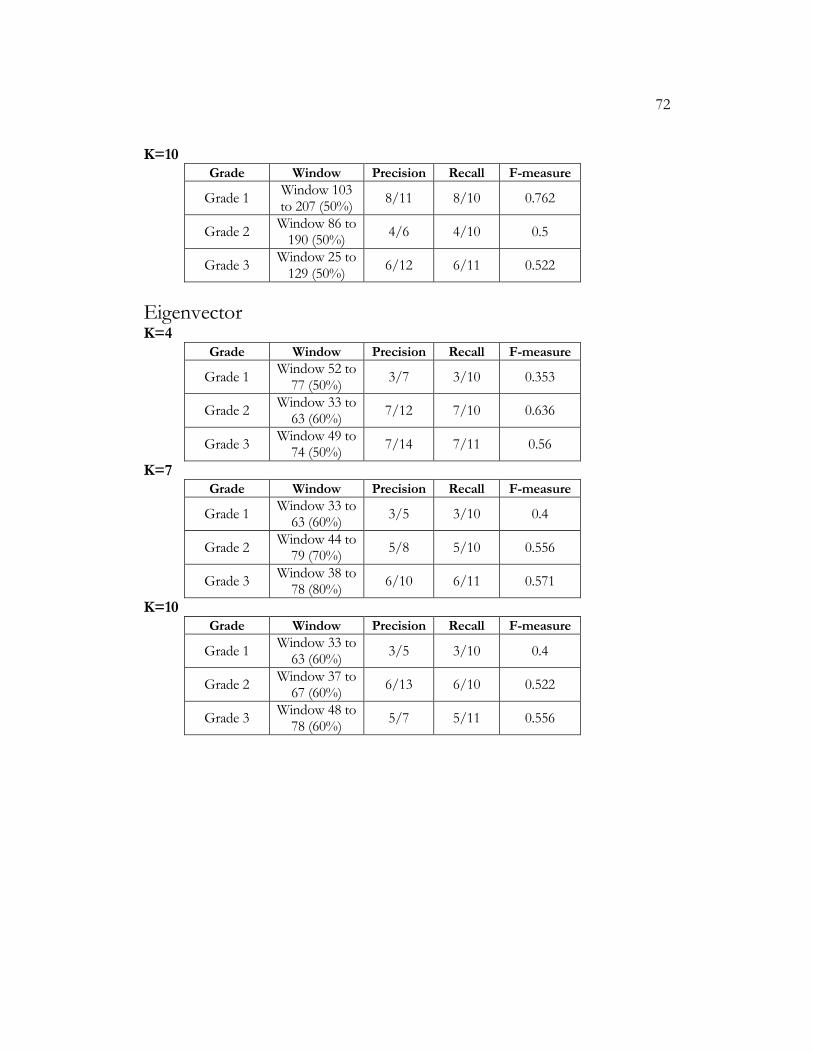
72

K=10 Grade Window Precision Recall F-measure

Grade 1 Window 103 to 207 (50%)

8/11 8/10 0.762

Grade 2 Window 86 to 190 (50%)

4/6 4/10 0.5

Grade 3 Window 25 to 129 (50%)

6/12 6/11 0.522

Eigenvector K=4

Grade Window Precision Recall F-measure

Grade 1 Window 52 to

77 (50%) 3/7 3/10 0.353

Grade 2 Window 33 to

63 (60%) 7/12 7/10 0.636

Grade 3 Window 49 to

74 (50%) 7/14 7/11 0.56

K=7 Grade Window Precision Recall F-measure

Grade 1 Window 33 to

63 (60%) 3/5 3/10 0.4

Grade 2 Window 44 to

79 (70%) 5/8 5/10 0.556

Grade 3 Window 38 to

78 (80%) 6/10 6/11 0.571

K=10 Grade Window Precision Recall F-measure

Grade 1 Window 33 to

63 (60%) 3/5 3/10 0.4

Grade 2 Window 37 to

67 (60%) 6/13 6/10 0.522

Grade 3 Window 48 to

78 (60%) 5/7 5/11 0.556

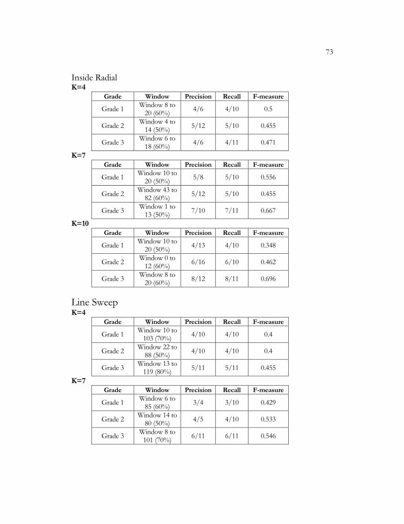
73

Inside Radial K=4

Grade Window Precision Recall F-measure

Grade 1 Window 8 to 20 (60%)

4/6 4/10 0.5

Grade 2 Window 4 to 14 (50%)

5/12 5/10 0.455

Grade 3 Window 6 to 18 (60%)

4/6 4/11 0.471

K=7 Grade Window Precision Recall F-measure

Grade 1 Window 10 to

20 (50%) 5/8 5/10 0.556

Grade 2 Window 43 to

82 (60%) 5/12 5/10 0.455

Grade 3 Window 1 to 13 (50%)

7/10 7/11 0.667

K=10 Grade Window Precision Recall F-measure

Grade 1 Window 10 to

20 (50%) 4/13 4/10 0.348

Grade 2 Window 0 to 12 (60%)

6/16 6/10 0.462

Grade 3 Window 8 to 20 (60%)

8/12 8/11 0.696

Line Sweep K=4

Grade Window Precision Recall F-measure

Grade 1 Window 10 to 103 (70%)

4/10 4/10 0.4

Grade 2 Window 22 to

88 (50%) 4/10 4/10 0.4

Grade 3 Window 13 to 119 (80%)

5/11 5/11 0.455

K=7 Grade Window Precision Recall F-measure

Grade 1 Window 6 to 85 (60%)

3/4 3/10 0.429

Grade 2 Window 14 to

80 (50%) 4/5 4/10 0.533

Grade 3 Window 8 to 101 (70%)

6/11 6/11 0.546

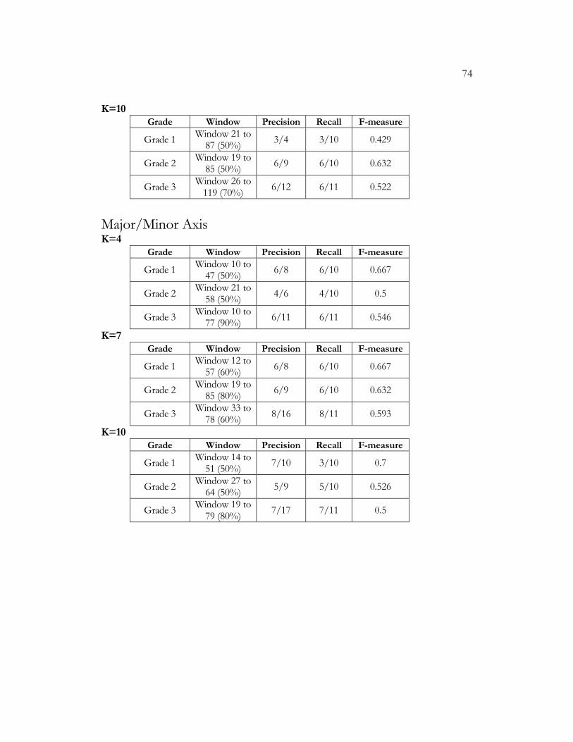
74

K=10 Grade Window Precision Recall F-measure

Grade 1 Window 21 to

87 (50%) 3/4 3/10 0.429

Grade 2 Window 19 to

85 (50%) 6/9 6/10 0.632

Grade 3 Window 26 to 119 (70%)

6/12 6/11 0.522

Major/Minor Axis K=4

Grade Window Precision Recall F-measure

Grade 1 Window 10 to

47 (50%) 6/8 6/10 0.667

Grade 2 Window 21 to

58 (50%) 4/6 4/10 0.5

Grade 3 Window 10 to

77 (90%) 6/11 6/11 0.546

K=7 Grade Window Precision Recall F-measure

Grade 1 Window 12 to

57 (60%) 6/8 6/10 0.667

Grade 2 Window 19 to

85 (80%) 6/9 6/10 0.632

Grade 3 Window 33 to

78 (60%) 8/16 8/11 0.593

K=10 Grade Window Precision Recall F-measure

Grade 1 Window 14 to

51 (50%) 7/10 3/10 0.7

Grade 2 Window 27 to

64 (50%) 5/9 5/10 0.526

Grade 3 Window 19 to

79 (80%) 7/17 7/11 0.5

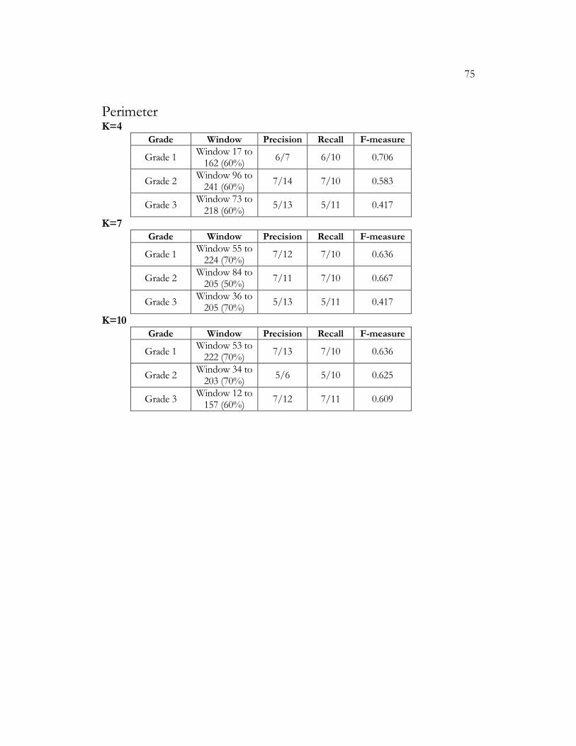
75

Perimeter K=4

Grade Window Precision Recall F-measure

Grade 1 Window 17 to 162 (60%)

6/7 6/10 0.706

Grade 2 Window 96 to 241 (60%)

7/14 7/10 0.583

Grade 3 Window 73 to 218 (60%)

5/13 5/11 0.417

K=7 Grade Window Precision Recall F-measure

Grade 1 Window 55 to 224 (70%)

7/12 7/10 0.636

Grade 2 Window 84 to 205 (50%)

7/11 7/10 0.667

Grade 3 Window 36 to 205 (70%)

5/13 5/11 0.417

K=10

Grade Window Precision Recall F-measure

Grade 1 Window 53 to 222 (70%)

7/13 7/10 0.636

Grade 2 Window 34 to 203 (70%)

5/6 5/10 0.625

Grade 3 Window 12 to 157 (60%)

7/12 7/11 0.609

76

A p p e n d i x B

ONLINE RESOURCES

For all data pertaining to all experiments please visit:

http://www.cs.drexel.edu/~jzz22/thesis . If any concerns regarding this thesis may

arise, please contact me at jzz22@drexel.edu.

77

LIST OF REFERENCES

1. J. Aßfalg, K. M. Borgwardt, H. Kriegel, 3DString: a feature string kernel for 3D object classification on voxelized data. Proceedings of the 15th ACM international Conference on information and Knowledge Management, 2006

2. P. H. Bartels, G.L. Wied, Computer analysis and biomedical interpretation of

microscopic images: Current problems and future directions, Proceedings of the IEEE , vol.65, no.2, pp. 252-261, 1977

3. Spotting medical mistakes, BBC News, June 13, 2000 4. G. Borgefors, Distance transformations in arbitrary dimensions, Computer Vision,

Graphics, and Image Processing, vol. 27, pp. 321-345, 1984 5. D. Breen, R. Fedkiw, K. Museth, S. Osher, G. Sapiro, R. Whitaker, Level set and

PDE methods for computer graphics. ACM SIGGRAPH 2004 Course Notes, 2004 6. J. E. Bresenham, Algorithm for computer control of a digital plotter, IBM Systems

Journal, vol. 4, 1, 1965 7. I. Carlbom, I. Chakravarty, W. M. Hsu. SIGGRAPH'91 Workshop Report

Integrating Computer Graphics, Computer Vision, and Image Processing in Scientific Applications, ACM SIG GRAPH Computer Graphics, Volume 26, Issue 1, 1992)

8. K. R. Castleman, Digtal Image Processing, Prentice Hall, 1996 9. C. Chambers, D. Ungar, Making pure object-oriented languages practical. Conference

Proceedings on Object-Oriented Programming Systems, Languages, and Applications, 1991 10. S. J. Colley, Vector Calculus, Prentice Hall, 2nd edition, 2002 11. L. F. Costa, R. M. Cesar Jr. Shape Analysis and Classification: Theory and Practice, CRC,

2000 12. W. J. Dally, J. T. Kajiya, An object oriented architecture. Proceedings of the 12th

Annual international Symposium on Computer Architecture, 1985 13. P. E. Danielsson, Euclidean distance mapping, CVGIP, vol. 14, pp. 227-248, 1980

78

14. M. Datar, D. Padfield, H. Cline. Color and Texture Based Segmentation of

Molecular Pathology Images using HSOMs, Proceedings of 2nd Workshop on Microsopic Image Analysis with Applications in Biology, 2007

15. J. L. Devore, Probability and Statistics for Engineering and the Sciences, Duxbury Press,

7th edition, 2007 16. S. Doyle, M. Hwang, K. Shah, A. Madabhushi, J. Tomasezweski, M. Feldman,

Automated Grading of Prostate Cancer using Architectural and Textural Image Features, International Symposium on Biomedical Imaging, pp. 1284-87, 2007

17. R. O. Duda, P. E. Hart, D. G. Stork, Pattern Classification, Wiley-Intersience; 2nd

edition, 2001 18. A. Elinson, D. S. Nau, W. C. Regli, Feature-based similarity assessment of solid

models. In Proceedings of the Fourth ACM Symposium on Solid Modeling and Applications, 1997

19. D. Freedman, T. Zhang, Interactive graph cut based segmentation with shape

priors, Computer Vision and Pattern Recognition, 2005. CVPR 2005. IEEE Computer Society Conference on , vol.1, no., pp. 755-762 vol. 1, 20-25 June 2005

20. T. Funkhouser, P. Min, M. Kazhdan, J. Chen, A. Halderman, D. Dobkin, D.

Jacobs, A search engine for 3D models. ACM Trans. Graph. vol. 22, 1, 2003 21. G. Golub and C. van Loan. Matrix Computations, The Johns Hopkins University

Press; 3rd edition, 1996 22. R. C. Gonzalez, R. E. Woods, S. L. Eddins. Digital Image Processing with Matlab,

Prentice Hall, 2004 23. S. K. Gupta, W. C. Regli, D. S. Nau, Manufacturing feature instances: which ones

to recognize?. Proceedings of the Third ACM Symposium on Solid Modeling and Applications, 1995

24. R. Haralick and L. Shapiro Computer and Robot Vision, Vol. 1, Chap. 5, Addison-

Wesley Publishing Company, 1992 25. U. Hölzle, D. Ungar, Reconciling responsiveness with performance in pure object-

oriented languages. ACM Trans. Program. Lang. Syst., 1996

79

26. B. K. P. Horn, Robot Vision, The MIT Press, 1986 27. M. H. Hueckel, A Local Visual Operator Which Recognizes Edges and Lines.

Journal of the ACM 20, 1973 28. 2007. Insight Toolkit (ITK).

http://www.itk.org 29. C. Ip and D. Lapadat and L. Sieger and W. Regli. Using shape distributions to

compare solid models, In Seventh ACM Symposium on Solid Modeling and Applications. ACM SIGGRAPH, ACM Press, Jun 17-23 2002.

30. A. Jain. Fundamentals of Digital Image Processing, Prentice-Hall, 1989 31. R. Jain and Y. Roth. Visualization and computer vision. Position paper for the

SIGGRAPH'91 Workshop on Integrating Computer Graphics, Computer Vision, and hnage Processing in Scientific Applications, 1991.

32. K. J. Khouzani, H. Soltanian-Zadeh, Automatic grading of pathological images of

prostate using multiwavelet transform, Engineering in Medicine and Biology Society, 2001. Proceedings of the 23rd Annual International Conference of the IEEE, 2545 - 2548 vol.3, 2001

33. H. M. Ladak, F. Mao; Y. Wang; D. B. Downey, D. A. Steinman, A. Fenster,

Prostate segmentation from 2D ultrasound images, Engineering in Medicine and Biology Society, 2000. Proceedings of the 22nd Annual International Conference of the IEEE, vol.4, pp.3188-3191, 2000

34. F. M. Lopes,. L. A.. Consularo, A RBFN Perceptive Model for Image

Thresholding, Computer Graphics and Image Processing, 2005. SIBGRAPI 2005. 18th Brazilian Symposium on , pp. 225-232, 2005

35. J. Makhoul, F. Kubala, R. Schwartz, R. Weischedel, Performance measures for

information extraction. Proceedings of DARPA Broadcast News Workshop, 1999 36. M. Masseroli, S. Bonacina, F. Pinciroli, Java-Based Browsing, Visualization and

Processing of Heterogeneous Medical Data from Remote Repositories," Engineering in Medicine and Biology Society, 2004. IEMBS '04. 26th Annual International Conference of the IEEE , vol.2, pp. 3326-3329, 2004

80

37. K. Minho, H. Yo-Sung, Semi-automatic segmentation by a double labeling method, TENCON 99. Proceedings of the IEEE Region 10 Conference , vol.1, pp.746-749, 1999

38. E. N. Mortensen, J. Jia, Real-Time Semi-Automatic Segmentation Using a Bayesian

Network, Computer Vision and Pattern Recognition, 2006 IEEE Computer Society Conference on , vol.1, pp. 1007-1014, 2006

39. D. Mumford, J. Shah. Optimal approximations by piecewise smooth functions and

associated variational problems, Communications on Pure and Applied Mathematics, Vol. XLII, pp 577-685, 1989

40. S. Naik, S. Doyle, M. Feldman, J. Tomaszewski, A. Madabhushi, Gland

Segmentation and Gleason Grading of Prostate Histology by Integrating Low-, High-level and Domain Specific Information, Proceedings of 2nd Workshop on Microsopic Image Analysis with Applications in Biology, 2007

41. K. Nandy, P.R. Gudla, S.J. Lockett. Automatic Segmentation of Cell Nuclei in 2D

Using Dynamic Programming, Proceedings of 2nd Workshop on Microsopic Image Analysis with Applications in Biology, 2007

42. R. Osada, T. Funkhouser, B. Chazelle, D. Dobkin, Shape distributions. ACM

Transaction on Graphics, vol. 21, 4, pp. 807-832, 2002 43. J. L. Pajon, V. Bui-Tran, and C. Bennis. Scientific visualization: A way of

reconciling experimentation and modeling. Position paper for the SIGGRAPH'91 Workshop on Integrating Computer Graphics, Computer Vision, and Image Processing in Scientific Applications, 1991.

44. M. Peabody, Finding Groups of Graphs in Databases, Master’s Thesis, Drexel

University, 2002 45. S. Petushi, C. Katsinis, C. Coward, F. Garcia, A. Tozeren, Automated

identification of microstructures on histology slides, Biomedical Imaging: Nano to Macro, 2004. IEEE International Symposium on , pp. 424-427 Vol. 1, 2004

46. S. Petushi, J. Marker, J. Zhang, W. Zhu, D. Breen, C. Chen, X. Lin, F.Garcia, A

Visual Analytics System for Breast Tumor Evaluation, Analytical and Quantitative Cytology and Histology , 2007

81

47. W. C. Regli, D. S. Nau, Building a general approach to feature recognition of Material Removal Shape Element Volumes (MRSEVs), Proceedings on the Second ACM Symposium on Solid Modeling and Applications, 1993

48. C. J. van Rijsbergen, Information Retrieval, Butterworth-Heinemann; 2Rev Ed

edition, March 1979 49. A. Rosenfeld, J. Pfaltz, Distance Functions in Digital Pictures, Pattern Recognition, Vol

1, pp 33-61, 1968 50. Y. Rubner, C. Tomasi. Perceptual Metrics for Image Database Navigation. Kluwer

Academic Publishers, Boston, December 2000 51. Y. Rubner, C. Tomasi, L. J. Guibas. The Earth Mover’s Distance as a Metric for

Image Retrieval, International Journal of Computer Vision 40(2), 99–121, 2000 52. J. A. Sethian. Level Set Methods and Fast Marching Methods, Cambridge University

Press; 2nd edition, 1999

53. N. L. Sizto, L. J. Dietz, Method and apparatus for cell counting and cell classification, US Patent: 5556764, 1994

54. G. Smith. Pathologist shortage hits small towns hard, Chicago Tribune, Oct. 11, 2007 55. G. Strang, Introduction to Linear Algebra, Wellesley-Cambridge, 2003 56. A. Verma, A. Kriete, Robust Object-Oriented Segmentation for High-Content

Screening, Proceedings of 2nd Workshop on Microsopic Image Analysis with Applications in Biology, 2007

57. A. R. Weeks, Fundamentals of Electronic Image Processing, Wiley-IEEE Press, 1996 58. G. Winkler, Image Analysis, Random Fields and Markov Chain Monte Carlo Methods: A

Mathematical Introduction, Springer-Verlag; 2nd edition, 2003