Embed Size (px)
Citation preview
Available online at www.sciencedirect.com
ScienceDirect
Journal of Functional Analysis 266 (2014) 1395–1420
www.elsevier.com/locate/jfa
An application of weighted Hardy spaces tothe Navier–Stokes equations
Yohei Tsutsui
Department of Mathematics, Faculty of Science and Engineering, Waseda University, Shinjuku, Tokyo 169-8555, Japan
Received 19 December 2012; accepted 3 December 2013
Available online 12 December 2013
Communicated by J. Bourgain
Abstract
In this article, we consider the mapping properties of convolution operators with smooth functions onweighted Hardy spaces Hp(w) with w belonging to Muckenhoupt class A∞. As a corollary, one obtainsdecay estimates of heat semigroup on weighted Hardy spaces. After a weighted version of the div–curllemma is established, these estimates on weighted Hardy spaces are applied to the investigation of the decayproperty of global mild solutions to Navier–Stokes equations with the initial data belonging to weightedHardy spaces.© 2013 Elsevier Inc. All rights reserved.
Keywords: Weighted Hardy spaces; Convolution operators; Div–curl lemma; Navier–Stokes equations
1. Introduction
Aims of this article are to establish estimates for the heat semigroup and div–curl estimateson weighted Hardy spaces and to investigate time decay of solutions to Navier–Stokes equationswith the initial data belonging to weighted Hardy spaces. Weights, we treat in this paper, belongto Muckenhoupt class A∞.
The first aim is to find a sufficient condition on weights that ensures the boundedness of con-volution operators with smooth functions on weighted Hardy spaces Hp(w), see Definition 1.2below, of the form:
‖f ∗ ϕ‖Hq(σ) � c‖f ‖Hp(w). (1)
E-mail address: [email protected].
0022-1236/$ – see front matter © 2013 Elsevier Inc. All rights reserved.http://dx.doi.org/10.1016/j.jfa.2013.12.002

1396 Y. Tsutsui / Journal of Functional Analysis 266 (2014) 1395–1420
The same inequalities on Lebesgue spaces with power weights were treated in [20] where theauthor assumed w ∈ Ap and σ ∈ Aq . Meanwhile, Theorem 1.1 below does not need such as-sumption on weights, also see Lemma 1.1. As a corollary of Theorem 1.1, Hp(| · |αp)−Hq(| · |βq)
estimates for the heat semigroup et� are given. Their decay order of t can be large as possible,see Corollary 1.1. This is one of advantages of the usage of weighted Hardy spaces insteadof weighted Lebesgue spaces. In the proof of Theorem 1.1, atomic decompositions by García-Cuerva [5] and Strömberg and Torchinsky [18], and the molecular characterization in Taiblesonand Weiss [19] and Lee and Lin [11] are applied.
Next aim is to establish the so-called “div–curl lemma” on weighted Hardy spaces. Div–curl lemma was proved by Coifman, Lions, Meyer and Semmes [3]: for divergence free vectorfields u
∥∥(u · ∇)v∥∥
Hr � ‖u‖Hp‖∇v‖Hq
where n/(n + 1) < p,q < ∞ and 1/r = 1/p + 1/q < 1 + 1/n. At the case p = ∞, Auscher,Russ and Tchamitchian [1] verified that the inequalities still hold. The proof of our div–curl lemma relies on a pointwise estimate of the grand maximal function of the bilinearform (u · ∇)v due to Miyachi [15] in the non-endpoint cases p < ∞ and the approach ofAuscher, Russ and Tchamitchian [1] in the endpoint case p = ∞, see Theorem 1.2 and The-orem 1.3.
Finally we investigate the time decay property of global solutions in Kato [10] to the incom-pressible homogeneous Navier–Stokes equations
(N–S)
⎧⎪⎨⎪⎩
∂tu − Δu + (u · ∇)u + ∇p = 0,
divu = 0,
u(0) = a
when the initial data a belongs to weighted Hardy spaces. Here u = (u1, . . . , un) is the unknownvelocity vector field, p is the unknown pressure scalar field and a = (a1, . . . , an) is the giveninitial velocity with diva = ∇ · a = 0. In this research, Theorem 1.1 is applied to the linearestimate and Theorems 1.2 and 1.3 are applied to control the non-linear term (u · ∇)u. Kato [10]and Giga and Miyakawa [7] showed if ‖a‖Ln is small and a ∈ Lp for some p ∈ (1,2), thenthe mild solution u has that ‖u(t)‖L2 � t−γ with γ = n(1/p − 1/2)/2. Wiegner [21] provedthat for θ � 0, if a ∈ L2 and ‖et�a‖L2 � t−θ (i.e. a ∈ B−2θ
2,∞ ), then the weak solution u has that‖u(t)‖L2 � t−γW with γW = min(θ, (n + 2)/4). Observe that γ < (n + 2)/4 ⇔ n/(n + 1) < p.We make γ be close to the critical order (n + 2)/4 of Wiegner with the aid of weighted Hardyspaces. But our analysis cannot reach to the critical order (n + 2)/4, see 2 of Remark 1.6.
The real variable theory of Hardy spaces was initiated by Fefferman and Stein [4], and then itsweighted version by García-Cuerva [5]. The fundamental properties of weighted Hardy spaces:density, duality, boundedness of Fourier multipliers, etc., were studied by Strömberg and Torchin-sky [18]. Two atomic decompositions with different notations of atom were given in [5] and [18],and will be applied to the proof of Theorem 1.1. Lee and Lin [11] gave a weighted version ofthe molecular characterization due to Taibleson and Weiss [19]. Our sufficient conditions for theboundedness of convolution operators are similar to that for the fractional integral operators inGatto, Gutiérrez and Wheeden [6].
Y. Tsutsui / Journal of Functional Analysis 266 (2014) 1395–1420 1397
For the application, we need a weighted version of so-called “div–curl lemma” due to Coif-man, Lions, Meyer and Semmes [3]. Our “div–curl lemma” in the non-endpoint case Theorem 1.2follows from the pointwise estimates of bilinear forms with the cancellation property by Miy-achi [15]. Since the proof uses the boundedness of the Riesz transforms, this method does notwork on the endpoint case. To get the div–curl lemma in the case Theorem 1.3, we apply anapproach by Auscher, Russ and Tchamitchian [1] which does not need such boundedness.
There are papers which studied the Navier–Stokes equations with Hardy spaces, for exampleMiyakawa [16] and [17]. Applying the theory of Hardy spaces seems to be natural, because thenon-linear term (u · ∇)u has the cancellation property:
∫(u · ∇)udx = 0 and then belongs to H 1
from “div–curl lemma” under the suitable assumption on the velocity u.To state our results, we begin with definitions of Muckenhoupt class and weighted Hardy
spaces.We say w is a “weight” if w is a non-negative and locally integrable function. For a subset
E ⊂ Rn, χE means the characteristic function of E and |E| the volume of E. Throughout thisarticle we use the following notations:
w(E) =∫E
w dx, 〈f 〉E = 1
|E|∫E
f dx, 〈f 〉E;w = 1
w(E)
∫E
f w dx.
By a “cube” Q we mean a cube in Rn with sides parallel to the coordinate axes. B(x, r) means anopen ball centered at x with radius r . We fix a smooth function Φ satisfying suppΦ ⊂ B(0,1),0 � Φ � 1, Φ ≡ 1 on B(0,1/2). We also use the notation Mr;wf (x) = supQ�x〈|f |r 〉1/r
Q;w , wherethe supremum is taken over all cubes Q containing x, and M denotes the Hardy–Littlewoodmaximal operator. A � B and A ≈ B mean A � c0B and c1B � Ac2B with positive constantsc0, c1 and c2. In what follows, c denotes a constant that is independent of the functions involved,which may differ from line to line.
Definition 1.1. A weight w is said to be in the Muckenhoupt class Ap (1 � p � ∞), if the Ap
constant [w]Ap is finite:
[w]A1 := supQ
〈w〉Q∥∥w−1
∥∥L∞(Q)
,
[w]Ap := supQ
〈w〉Q⟨w1−p′ ⟩p−1
Q(1 < p < ∞),
and
[w]A∞ := supQ
〈w〉Q exp(⟨
logw−1⟩Q
),
where the suprema are taken over all cubes Q. Also, we define qw := inf{q ∈ [1,∞); w ∈ Aq}.It is well known that w(x) = |x|α ∈ Ap if and only if −n < α � 0 when p = 1 and −n < α <
n(p − 1) when p > 1.
Remark 1.1.
1. [w]Ap � 1 and 1 � p < q � ∞ ⇒ Ap � Aq .
1398 Y. Tsutsui / Journal of Functional Analysis 266 (2014) 1395–1420
2. Ap classes have the openness property: if p ∈ (1,∞] and w ∈ Ap , there exists q ∈ (1,p) sothat w ∈ Aq .
3. w /∈ Aqw , if qw > 1.
It is well known that all A∞ weights satisfy the reverse Hölder inequality. In a recent studyof the sharp weighted inequalities for Calderón–Zygmund operators, the optimal orders of thereverse Hölder inequality were found by Lerner, Ombrosi and Pérez [13] for Ap weights withp < ∞ and Hytönen and Pérez [9] for A∞ weights.
Proposition A. (See [9].) Every w ∈ A∞ satisfy the “reverse Hölder inequality”:
⟨wrw
⟩1/rwQ
� 2〈w〉Q,
with rw := 1 + 12n+11‖w‖A∞
, where ‖w‖A∞ is another A∞ constant of w, see [9] for example.
The weighted Hardy spaces Hp(w) with w ∈ A∞ are defined as follows.
Definition 1.2. Let 0 < p � ∞ and w ∈ A∞. Define Hp(w) as a space of all tempered distribu-tions f whose the maximal function MΦf (x) = supt>0 |f ∗ Φt(x)| belongs to Lp(w), and
‖f ‖Hp(w) := ‖MΦf ‖Lp(w),
where L∞(w) denotes L∞.
Remark 1.2. It is well known that when 1 < p < ∞ and w ∈ Ap , it holds Hp(w) = Lp(w). Onthe other hand, if Lp(w) = Hp(w), then w has to belong to Ap . This fact also is true for opensubsets in Rn, see [14]. Furthermore, if 1 � p < q , then there is a w ∈ Aq so that the Dirac massbelongs to Hp(w), see p. 86 in [18].
In [18], several characterizations of Hp(w) by maximal functions, for example the grandmaximal function f ∗
m, were established. This maximal function is defined as follows: for m ∈N∪ {0}, x ∈ Rn and t ∈ (0,∞), Im(x, t) denotes a space of all function ψ ∈ C∞(B(x, t)) with
∥∥∂αψ∥∥
L∞ � t−(n+|α|) for |α| � m.
The grand maximal function f ∗m is then defined by
f ∗m(x) = sup
{∣∣f (ψ)∣∣; ψ ∈
⋃t∈(0,∞)
Im(x, t)
}.
We denote by D0 the set of all f ∈ S with f belonging to D and vanishing in a neighborhood ofξ = 0, where f means the Fourier transform of f . Strömberg and Torchinsky [18] proved thatD0 is a dense subspace of Hp(w) for p ∈ (0,∞) and doubling measures w.
Our first result of the paper reads as follows.
Y. Tsutsui / Journal of Functional Analysis 266 (2014) 1395–1420 1399
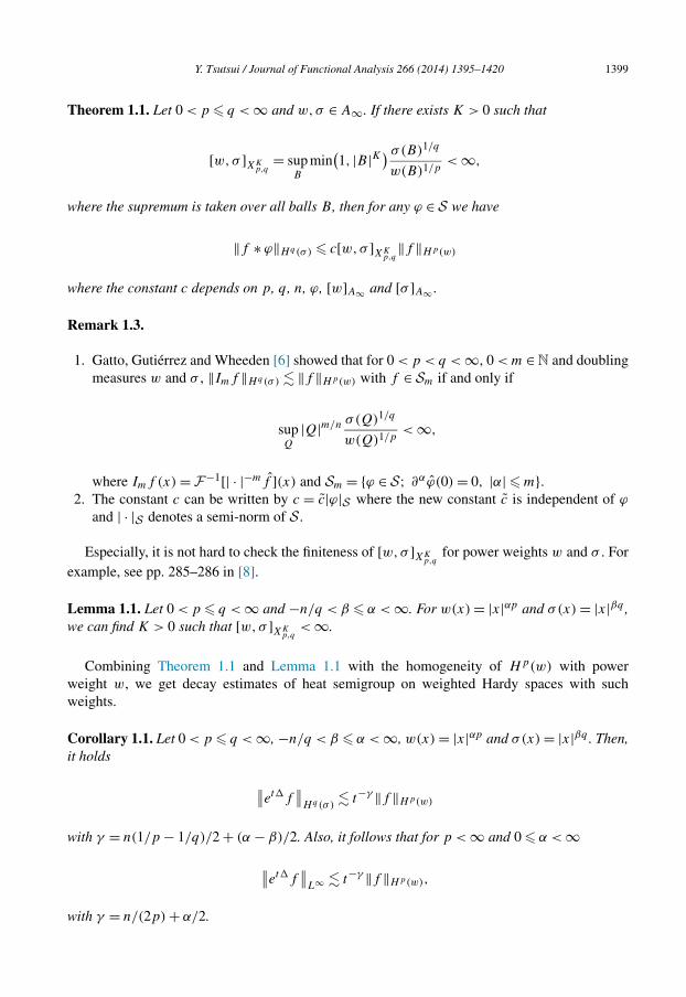
Theorem 1.1. Let 0 < p � q < ∞ and w,σ ∈ A∞. If there exists K > 0 such that
[w,σ ]XKp,q
= supB
min(1, |B|K) σ(B)1/q
w(B)1/p< ∞,
where the supremum is taken over all balls B , then for any ϕ ∈ S we have
‖f ∗ ϕ‖Hq(σ) � c[w,σ ]XKp,q
‖f ‖Hp(w)
where the constant c depends on p, q , n, ϕ, [w]A∞ and [σ ]A∞ .
Remark 1.3.
1. Gatto, Gutiérrez and Wheeden [6] showed that for 0 < p < q < ∞, 0 < m ∈ N and doublingmeasures w and σ , ‖Imf ‖Hq(σ) � ‖f ‖Hp(w) with f ∈ Sm if and only if
supQ
|Q|m/n σ (Q)1/q
w(Q)1/p< ∞,
where Imf (x) =F−1[| · |−mf ](x) and Sm = {ϕ ∈ S; ∂αϕ(0) = 0, |α| � m}.2. The constant c can be written by c = c|ϕ|S where the new constant c is independent of ϕ
and | · |S denotes a semi-norm of S .
Especially, it is not hard to check the finiteness of [w,σ ]XKp,q
for power weights w and σ . Forexample, see pp. 285–286 in [8].
Lemma 1.1. Let 0 < p � q < ∞ and −n/q < β � α < ∞. For w(x) = |x|αp and σ(x) = |x|βq ,we can find K > 0 such that [w,σ ]XK
p,q< ∞.
Combining Theorem 1.1 and Lemma 1.1 with the homogeneity of Hp(w) with powerweight w, we get decay estimates of heat semigroup on weighted Hardy spaces with suchweights.
Corollary 1.1. Let 0 < p � q < ∞, −n/q < β � α < ∞, w(x) = |x|αp and σ(x) = |x|βq . Then,it holds
∥∥et�f∥∥
Hq(σ)� t−γ ‖f ‖Hp(w)
with γ = n(1/p − 1/q)/2 + (α − β)/2. Also, it follows that for p < ∞ and 0 � α < ∞∥∥et�f
∥∥L∞ � t−γ ‖f ‖Hp(w),
with γ = n/(2p) + α/2.
1400 Y. Tsutsui / Journal of Functional Analysis 266 (2014) 1395–1420
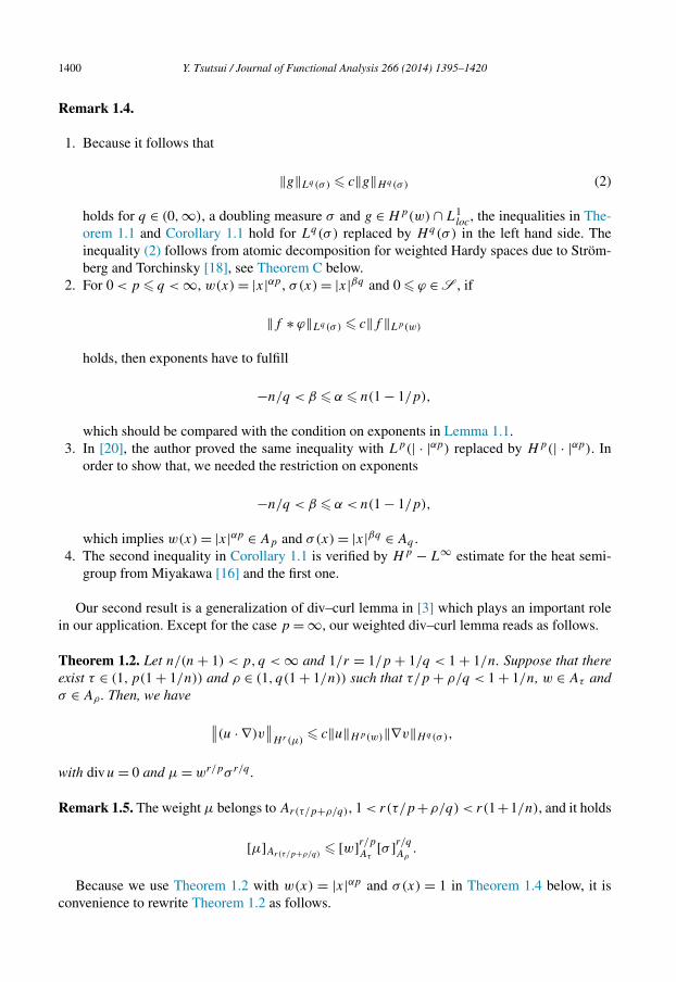
Remark 1.4.
1. Because it follows that
‖g‖Lq(σ ) � c‖g‖Hq(σ) (2)
holds for q ∈ (0,∞), a doubling measure σ and g ∈ Hp(w) ∩ L1loc, the inequalities in The-
orem 1.1 and Corollary 1.1 hold for Lq(σ ) replaced by Hq(σ) in the left hand side. Theinequality (2) follows from atomic decomposition for weighted Hardy spaces due to Ström-berg and Torchinsky [18], see Theorem C below.
2. For 0 < p � q < ∞, w(x) = |x|αp , σ(x) = |x|βq and 0 � ϕ ∈ S , if
‖f ∗ ϕ‖Lq(σ ) � c‖f ‖Lp(w)
holds, then exponents have to fulfill
−n/q < β � α � n(1 − 1/p),
which should be compared with the condition on exponents in Lemma 1.1.3. In [20], the author proved the same inequality with Lp(| · |αp) replaced by Hp(| · |αp). In
order to show that, we needed the restriction on exponents
−n/q < β � α < n(1 − 1/p),
which implies w(x) = |x|αp ∈ Ap and σ(x) = |x|βq ∈ Aq .4. The second inequality in Corollary 1.1 is verified by Hp − L∞ estimate for the heat semi-
group from Miyakawa [16] and the first one.
Our second result is a generalization of div–curl lemma in [3] which plays an important rolein our application. Except for the case p = ∞, our weighted div–curl lemma reads as follows.
Theorem 1.2. Let n/(n + 1) < p,q < ∞ and 1/r = 1/p + 1/q < 1 + 1/n. Suppose that thereexist τ ∈ (1,p(1 + 1/n)) and ρ ∈ (1, q(1 + 1/n)) such that τ/p + ρ/q < 1 + 1/n, w ∈ Aτ andσ ∈ Aρ . Then, we have
∥∥(u · ∇)v∥∥
Hr(μ)� c‖u‖Hp(w)‖∇v‖Hq(σ),
with divu = 0 and μ = wr/pσ r/q .
Remark 1.5. The weight μ belongs to Ar(τ/p+ρ/q), 1 < r(τ/p+ρ/q) < r(1+1/n), and it holds
[μ]Ar(τ/p+ρ/q)� [w]r/pAτ
[σ ]r/qAρ.
Because we use Theorem 1.2 with w(x) = |x|αp and σ(x) = 1 in Theorem 1.4 below, it isconvenience to rewrite Theorem 1.2 as follows.
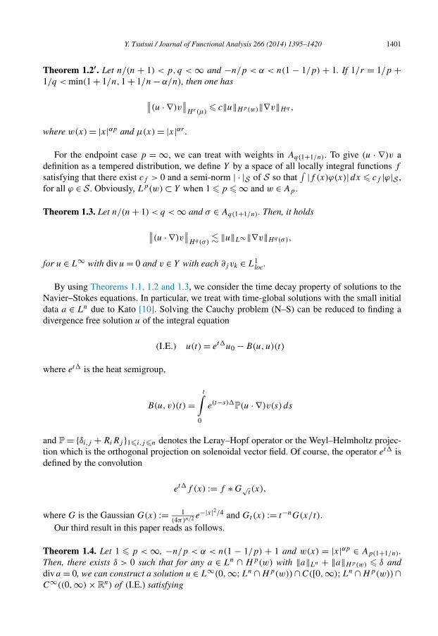
Y. Tsutsui / Journal of Functional Analysis 266 (2014) 1395–1420 1401
Theorem 1.2′. Let n/(n + 1) < p,q < ∞ and −n/p < α < n(1 − 1/p) + 1. If 1/r = 1/p +1/q < min(1 + 1/n,1 + 1/n − α/n), then one has
∥∥(u · ∇)v∥∥
Hr(μ)� c‖u‖Hp(w)‖∇v‖Hq ,
where w(x) = |x|αp and μ(x) = |x|αr .
For the endpoint case p = ∞, we can treat with weights in Aq(1+1/n). To give (u · ∇)v adefinition as a tempered distribution, we define Y by a space of all locally integral functions f
satisfying that there exist cf > 0 and a semi-norm | · |S of S so that∫ |f (x)ϕ(x)|dx � cf |ϕ|S ,
for all ϕ ∈ S . Obviously, Lp(w) ⊂ Y when 1 � p � ∞ and w ∈ Ap .
Theorem 1.3. Let n/(n + 1) < q < ∞ and σ ∈ Aq(1+1/n). Then, it holds
∥∥(u · ∇)v∥∥
Hq(σ)� ‖u‖L∞‖∇v‖Hq(σ),
for u ∈ L∞ with divu = 0 and v ∈ Y with each ∂j vk ∈ L1loc.
By using Theorems 1.1, 1.2 and 1.3, we consider the time decay property of solutions to theNavier–Stokes equations. In particular, we treat with time-global solutions with the small initialdata a ∈ Ln due to Kato [10]. Solving the Cauchy problem (N–S) can be reduced to finding adivergence free solution u of the integral equation
(I.E.) u(t) = et�u0 − B(u,u)(t)
where et� is the heat semigroup,
B(u, v)(t) =t∫
0
e(t−s)�P(u · ∇)v(s) ds
and P = {δi,j + RiRj }1�i,j�n denotes the Leray–Hopf operator or the Weyl–Helmholtz projec-tion which is the orthogonal projection on solenoidal vector field. Of course, the operator et� isdefined by the convolution
et�f (x) := f ∗ G√t (x),
where G is the Gaussian G(x) := 1(4π)n/2 e−|x|2/4 and Gt(x) := t−nG(x/t).
Our third result in this paper reads as follows.
Theorem 1.4. Let 1 � p < ∞, −n/p < α < n(1 − 1/p) + 1 and w(x) = |x|αp ∈ Ap(1+1/n).Then, there exists δ > 0 such that for any a ∈ Ln ∩ Hp(w) with ‖a‖Ln + ‖a‖Hp(w) � δ anddiva = 0, we can construct a solution u ∈ L∞(0,∞;Ln ∩Hp(w))∩C([0,∞);Ln ∩Hp(w))∩C∞((0,∞) ×Rn) of (I.E.) satisfying
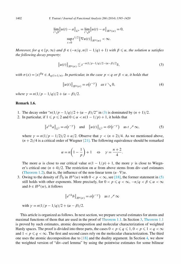
1402 Y. Tsutsui / Journal of Functional Analysis 266 (2014) 1395–1420
limt↘0
∥∥u(t) − a∥∥
Ln = limt↘0
∥∥u(t) − a∥∥
Hp(w)= 0,
supt>0
t1/2∥∥∇u(t)
∥∥Hp(w)
< ∞.
Moreover, for q ∈ [p,∞) and β ∈ (−n/q,n(1 − 1/q) + 1) with β � α, the solution u satisfiesthe following decay property:
∥∥u(t)∥∥
Hq(σ)� t−n(1/p−1/q)/2−(α−β)/2δ, (3)
with σ(x) = |x|βq ∈ Aq(1+1/n). In particular, in the case p < q or β < α, it holds that
∥∥u(t)∥∥
Hq(σ)= o
(t−γ
)as t ↘ 0, (4)
where γ = n(1/p − 1/q)/2 + (α − β)/2.
Remark 1.6.
1. The decay order “n(1/p − 1/q)/2 + (α − β)/2” in (3) is dominated by (n + 1)/2.2. In particular, if 1 � p � 2 and 0 � α < n(1 − 1/p) + 1, it holds that
∥∥et�a∥∥
L2 = o(t−γ
)and
∥∥u(t)∥∥
L2 = O(t−γ
)as t ↗ ∞, (5)
where γ = n(1/p − 1/2)/2 + α/2. Observe that γ < (n + 2)/4. As we mentioned above,(n + 2)/4 is a critical order of Wiegner [21]. The following equivalence should be remarked
α = n
(1 − 1
p
)+ 1 ⇔ γ = n + 2
4.
The more α is close to our critical value n(1 − 1/p) + 1, the more γ is close to Wiegn-er’s critical one (n + 4)/2. The restriction on α from above stems from div–curl estimates(Theorem 1.2), that is, the influence of the non-linear term (u · ∇)u.
3. Owing to the density of D0 in Hp(w) with 0 < p < ∞, see [18], the former statement in (5)still holds with other exponents. More precisely, for 0 < p � q < ∞, −n/q < β � α < ∞and b ∈ Hp(w), it follows
∥∥et�b∥∥
Hq(σ)= o
(t−γ
)as t ↗ ∞
with γ = n(1/p − 1/q)/2 + (α − β)/2.
This article is organized as follows. In next section, we prepare several estimates for atoms andmaximal functions of them that are used in the proof of Theorem 1.1. In Section 3, Theorem 1.1is proved by such estimates, atomic decomposition and molecular characterization of weightedHardy spaces. The proof is divided into three parts, the cases 0 < p � q � 1, 0 < p � 1 < q < ∞and 1 < p � q < ∞. The first and second cases rely on the molecular characterization. The thirdone uses the atomic decomposition due to [18] and the duality argument. In Section 4, we showthe weighted version of “div–curl lemma” by using the pointwise estimates for some bilinear
Y. Tsutsui / Journal of Functional Analysis 266 (2014) 1395–1420 1403
forms due to Miyachi [15] and an argument in [1]. Finally, in Section 5, we apply results inprevious sections to get the time decay estimates of solutions to Navier–Stokes equations withthe small initial data a ∈ Ln ∩ Hp(w).
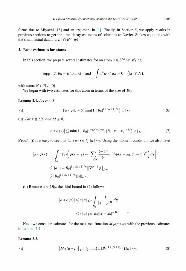
2. Basic estimates for atoms
In this section, we prepare several estimates for an atom a ∈ L∞ satisfying
suppa ⊂ B0 = B(x0, r0) and∫
xαa(x) dx = 0(|α| �N
),
with some N ∈ N∪ {0}.We begin with two estimates for this atom in terms of the size of B0.
Lemma 2.1. Let ϕ ∈ S .
(i) ‖a ∗ ϕ‖L∞ � min(1, |B0|1+(N+1)/n
)‖a‖L∞ . (6)
(ii) For x /∈ 2B0 and M � 0,
∣∣a ∗ ϕ(x)∣∣ � min
(1, |B0|1+(N+1)/n, |B0||x − x0|−M
)‖a‖L∞ . (7)
Proof. (i) It is easy to see that ‖a ∗ ϕ‖L∞ � ‖a‖L∞ . Using the moment condition, we also have
∣∣a ∗ ϕ(x)∣∣ =
∣∣∣∣∫B0
a(y)
(ϕ(x − y) −
∑|γ |�N
(−1)γ
γ ! ∂ |γ |φ(x − x0)(y − x0)γ
)dy
∣∣∣∣� ‖a‖L∞|B0|1+(N+1)/n
∥∥∇N+1ϕ∥∥
L∞
� |B0|1+(N+1)/n‖a‖L∞ .
(ii) Because x /∈ 2B0, the third bound in (7) follows:
∣∣a ∗ ϕ(x)∣∣ � c‖a‖L∞
∫B0
1
|x − y|M dy
� c‖a‖L∞|B0||x − x0|−M. �Next, we consider estimates for the maximal function MΦ(a ∗ ϕ) with the previous estimates
in Lemma 2.1.
Lemma 2.2.
(i)∥∥MΦ(a ∗ ϕ)
∥∥L∞ � min
(1, |B0|1+(N+1)/n
)‖a‖L∞ . (8)
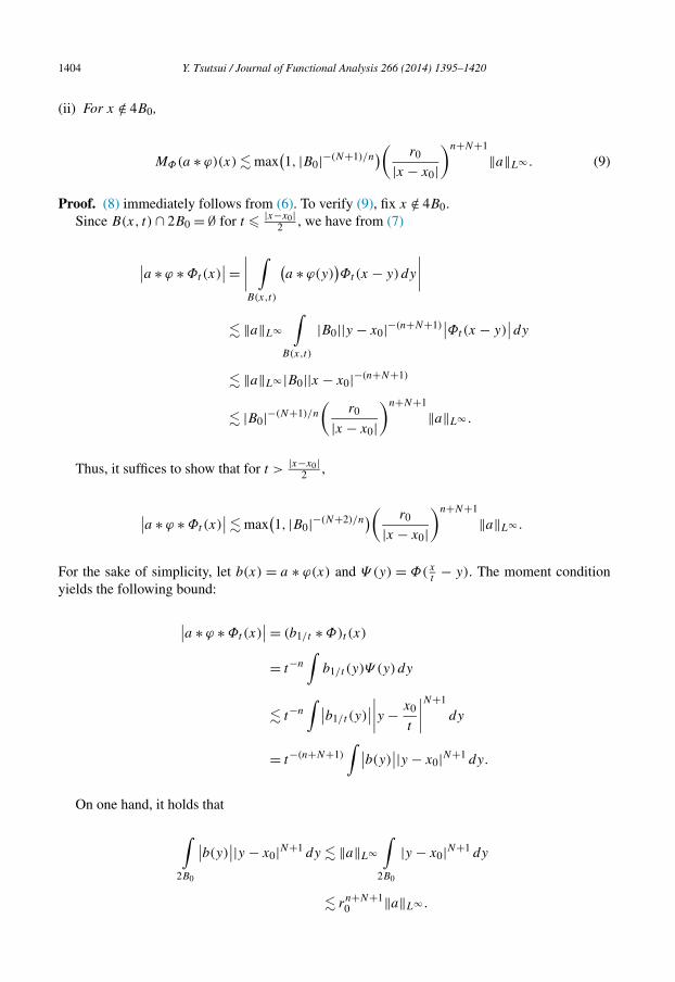
1404 Y. Tsutsui / Journal of Functional Analysis 266 (2014) 1395–1420
(ii) For x /∈ 4B0,
MΦ(a ∗ ϕ)(x) � max(1, |B0|−(N+1)/n
)( r0
|x − x0|)n+N+1
‖a‖L∞ . (9)
Proof. (8) immediately follows from (6). To verify (9), fix x /∈ 4B0.Since B(x, t) ∩ 2B0 = ∅ for t � |x−x0|
2 , we have from (7)
∣∣a ∗ ϕ ∗ Φt(x)∣∣ =
∣∣∣∣∫
B(x,t)
(a ∗ ϕ(y)
)Φt(x − y)dy
∣∣∣∣� ‖a‖L∞
∫B(x,t)
|B0||y − x0|−(n+N+1)∣∣Φt(x − y)
∣∣dy
� ‖a‖L∞|B0||x − x0|−(n+N+1)
� |B0|−(N+1)/n
(r0
|x − x0|)n+N+1
‖a‖L∞ .
Thus, it suffices to show that for t >|x−x0|
2 ,
∣∣a ∗ ϕ ∗ Φt(x)∣∣ � max
(1, |B0|−(N+2)/n
)( r0
|x − x0|)n+N+1
‖a‖L∞ .
For the sake of simplicity, let b(x) = a ∗ ϕ(x) and Ψ (y) = Φ(xt
− y). The moment conditionyields the following bound:
∣∣a ∗ ϕ ∗ Φt(x)∣∣ = (b1/t ∗ Φ)t (x)
= t−n
∫b1/t (y)Ψ (y)dy
� t−n
∫ ∣∣b1/t (y)∣∣∣∣∣∣y − x0
t
∣∣∣∣N+1
dy
= t−(n+N+1)
∫ ∣∣b(y)∣∣|y − x0|N+1 dy.
On one hand, it holds that
∫2B0
∣∣b(y)∣∣|y − x0|N+1 dy � ‖a‖L∞
∫2B0
|y − x0|N+1 dy
� rn+N+1‖a‖L∞ .
0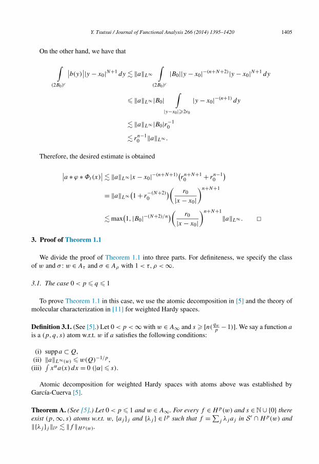
Y. Tsutsui / Journal of Functional Analysis 266 (2014) 1395–1420 1405
On the other hand, we have that
∫(2B0)
c
∣∣b(y)∣∣|y − x0|N+1 dy � ‖a‖L∞
∫(2B0)
c
|B0||y − x0|−(n+N+2)|y − x0|N+1 dy
� ‖a‖L∞|B0|∫
|y−x0|�2r0
|y − x0|−(n+1) dy
� ‖a‖L∞|B0|r−10
� rn−10 ‖a‖L∞ .
Therefore, the desired estimate is obtained
∣∣a ∗ ϕ ∗ Φt(x)∣∣ � ‖a‖L∞|x − x0|−(n+N+1)
(rn+N+1
0 + rn−10
)= ‖a‖L∞
(1 + r
−(N+2)0
)( r0
|x − x0|)n+N+1
� max(1, |B0|−(N+2)/n
)( r0
|x − x0|)n+N+1
‖a‖L∞ . �3. Proof of Theorem 1.1
We divide the proof of Theorem 1.1 into three parts. For definiteness, we specify the classof w and σ : w ∈ Aτ and σ ∈ Aρ with 1 < τ,ρ < ∞.
3.1. The case 0 < p � q � 1
To prove Theorem 1.1 in this case, we use the atomic decomposition in [5] and the theory ofmolecular characterization in [11] for weighted Hardy spaces.
Definition 3.1. (See [5].) Let 0 < p < ∞ with w ∈ A∞ and s � [n(qw
p−1)]. We say a function a
is a (p, q, s) atom w.r.t. w if a satisfies the following conditions:
(i) suppa ⊂ Q,(ii) ‖a‖L∞(w) � w(Q)−1/p ,
(iii)∫
xαa(x) dx = 0 (|α| � s).
Atomic decomposition for weighted Hardy spaces with atoms above was established byGarcía-Cuerva [5].
Theorem A. (See [5].) Let 0 < p � 1 and w ∈ A∞. For every f ∈ Hp(w) and s ∈N∪ {0} thereexist (p,∞, s) atoms w.r.t. w, {aj }j and {λj } ∈ lp such that f = ∑
j λj aj in S ′ ∩ Hp(w) and‖{λj }j‖lp � ‖f ‖Hp(w).

1406 Y. Tsutsui / Journal of Functional Analysis 266 (2014) 1395–1420
The concept of molecule was introduced by Taibleson and Weiss [19], in which the char-acterization with molecules was given. The weighted version of it was studied by Lee andLin [11].
Definition 3.2. (See [19,11].) Let 0 < p � 1, w ∈ A∞. Suppose that
s �[n
(qw
p− 1
)], ε > max
(srw
n(rw − 1)+ 1
rw − 1,
1
p− 1
),
a = 1−1/p+ε and b = 1+ε (a, b > 0). Then, a function M is said to be a (p,∞, s, ε)-moleculew.r.t. w centered at x0 if M satisfies the following conditions:
(i) M(·)w(B(x0, | · −x0|))b ∈ L∞,(ii) Nw(M) := ‖M‖a/b
L∞(w)‖M(·)w(B(x0, | · −x0|))b‖1−a/bL∞ < ∞,
(iii)∫
xαM(x)dx = 0 (|α| � s).
The condition on ε above is used for the next Theorem B only.To investigate the mapping property for several linear operators, the following theorem is
useful.
Theorem B. (See [11].) Let 0 < p � 1 and s � [n(qw
p− 1)]. Assume that
ε > max
(srw
n(rw − 1)+ 1
rw − 1,
1
p− 1
),
a = 1−1/p+ε and b = 1+ε. For any M , (p,∞, s, ε)-molecule w.r.t. w, ‖M‖Hp(w) �Nw(M).
Proof of Theorem 1.1 in the case 0 < p ��� q ��� 1. From Theorem A, f ∈ Hp(w) can be decom-posed as f = ∑
j λj aj with suppaj ⊂ Bj = B(xj , rj ) and∫
xαaj (x) dx = 0 (|α| � N) with asufficiently large N . Since
‖f ∗ ϕ‖Hq(σ) �( ∞∑
j=1
|λj |q‖aj ∗ ϕ‖q
Hq(σ )
)1/q
,
it is sufficient to prove that
(I) {aj ∗ ϕ}j are (q,∞, N, ε)-molecules w.r.t. σ , where
N =[n
(qσ
q− 1
)]and ε > max
(Nrσ
n(rσ − 1)+ 1
rσ − 1,
1
q− 1
),
(II) supj
Nσ (aj ∗ ϕ)� [w,σ ]XKp,q
.
The moment condition in (I) is easily checked.
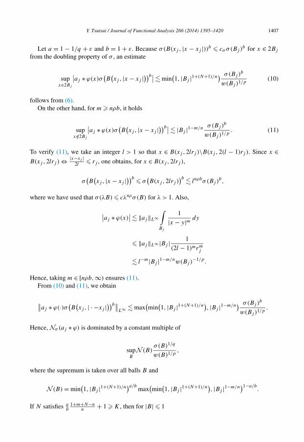
Y. Tsutsui / Journal of Functional Analysis 266 (2014) 1395–1420 1407
Let a = 1 − 1/q + ε and b = 1 + ε. Because σ(B(xj , |x − xj |))b � cσ σ (Bj )b for x ∈ 2Bj
from the doubling property of σ , an estimate
supx∈2Bj
∣∣aj ∗ ϕ(x)σ(B
(xj , |x − xj |
))b∣∣� min(1, |Bj |1+(N+1)/n
) σ(Bj )b
w(Bj )1/p(10)
follows from (6).On the other hand, for m � nρb, it holds
supx /∈2Bj
∣∣aj ∗ ϕ(x)σ(B
(xj , |x − xj |
))b∣∣� |Bj |1−m/n σ (Bj )b
w(Bj )1/p. (11)
To verify (11), we take an integer l > 1 so that x ∈ B(xj ,2lrj )\B(xj ,2(l − 1)rj ). Since x ∈B(xj ,2lrj ) ⇔ |x−xj |
2l� rj , one obtains, for x ∈ B(xj ,2lrj ),
σ(B
(xj , |x − xj |
))b � σ(B(xj ,2lrj )
)b � lnρbσ (Bj )b,
where we have used that σ(λB) � cλnρσ (B) for λ > 1. Also,
∣∣aj ∗ ϕ(x)∣∣ � ‖aj‖L∞
∫Bj
1
|x − y|m dy
� ‖aj‖L∞|Bj | 1
(2l − 1)mrmj
� l−m|Bj |1−m/nw(Bj )−1/p.
Hence, taking m ∈ [nρb,∞) ensures (11).From (10) and (11), we obtain
∥∥aj ∗ ϕ(·)σ (B
(xj , | · −xj |
))b∥∥L∞ � max
(min
(1, |Bj |1+(N+1)/n
), |Bj |1−m/n
) σ(Bj )b
w(Bj )1/p.
Hence, Nσ (aj ∗ ϕ) is dominated by a constant multiple of
supB
N (B)σ (B)1/q
w(B)1/p,
where the supremum is taken over all balls B and
N (B) = min(1, |Bj |1+(N+1)/n
)a/b max(min
(1, |Bj |1+(N+1)/n
), |Bj |1−m/n
)1−a/b.
If N satisfies a 1+m+N−n + 1 �K , then for |B| � 1
b n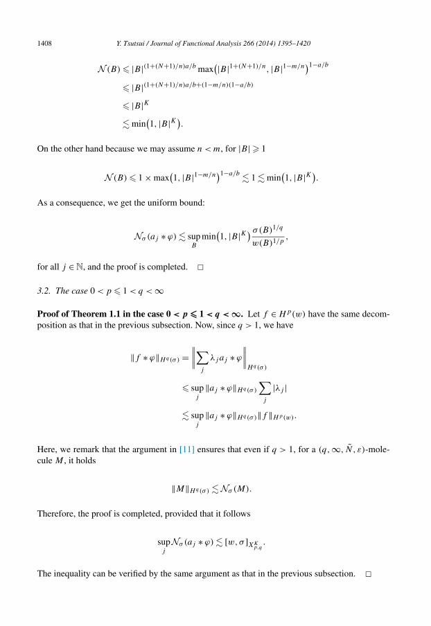
1408 Y. Tsutsui / Journal of Functional Analysis 266 (2014) 1395–1420
N (B) � |B|(1+(N+1)/n)a/b max(|B|1+(N+1)/n, |B|1−m/n
)1−a/b
� |B|(1+(N+1)/n)a/b+(1−m/n)(1−a/b)
� |B|K
� min(1, |B|K)
.
On the other hand because we may assume n < m, for |B| � 1
N (B) � 1 × max(1, |B|1−m/n
)1−a/b � 1 � min(1, |B|K)
.
As a consequence, we get the uniform bound:
Nσ (aj ∗ ϕ) � supB
min(1, |B|K) σ(B)1/q
w(B)1/p,
for all j ∈N, and the proof is completed. �3.2. The case 0 < p � 1 < q < ∞
Proof of Theorem 1.1 in the case 0 < p ��� 1 < q < ∞. Let f ∈ Hp(w) have the same decom-position as that in the previous subsection. Now, since q > 1, we have
‖f ∗ ϕ‖Hq(σ) =∥∥∥∥∑
j
λjaj ∗ ϕ
∥∥∥∥Hq(σ)
� supj
‖aj ∗ ϕ‖Hq(σ)
∑j
|λj |
� supj
‖aj ∗ ϕ‖Hq(σ)‖f ‖Hp(w).
Here, we remark that the argument in [11] ensures that even if q > 1, for a (q,∞, N, ε)-mole-cule M , it holds
‖M‖Hq(σ) �Nσ (M).
Therefore, the proof is completed, provided that it follows
supj
Nσ (aj ∗ ϕ)� [w,σ ]XKp,q
.
The inequality can be verified by the same argument as that in the previous subsection. �
Y. Tsutsui / Journal of Functional Analysis 266 (2014) 1395–1420 1409
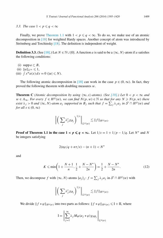
3.3. The case 1 < p � q < ∞
Finally, we prove Theorem 1.1 with 1 < p � q < ∞. To do so, we make use of an atomicdecomposition in [18] for weighted Hardy spaces. Another concept of atom was introduced byStrömberg and Torchinsky [18]. The definition is independent of weight.
Definition 3.3. (See [18].) Let N ∈N∪{0}. A function a is said to be a 〈∞,N〉-atom if a satisfiesthe following conditions:
(i) suppa ⊂ B ,(ii) ‖a‖L∞ � 1,
(iii)∫
xαa(x) dx = 0 (|α| �N).
The following atomic decomposition in [18] can work in the case p ∈ (0,∞). In fact, theyproved the following theorem with doubling measures w.
Theorem C (Atomic decomposition by using 〈∞, s〉-atoms). (See [18].) Let 0 < p < ∞ andw ∈ A∞. For every f ∈ Hp(w), we can find N(p,w) ∈ N so that for any N � N(p,w) thereexist λj > 0 and 〈∞,N〉-atom aj supported in Bj such that f = ∑
j λjaj in S ′ ∩ Hp(w) andfor all s ∈ (0,∞)
∥∥∥∥( ∑
j
λsjχBj
)1/s∥∥∥∥Lp(w)
� ‖f ‖Hp(w).
Proof of Theorem 1.1 in the case 1 < p ��� q < ∞. Let 1/s = 1 + 1/p − 1/q . Let N∗ and N
be integers satisfying
2(nρ/q + nτ/s) − (n + 1) < N∗
and
K � min
(1 + N + 1
n,
1
2+ N − N∗
2n
)= 1
2+ N − N∗
2n. (12)
Then, we decompose f with 〈∞,N〉-atoms {aj }j : f = ∑j λj aj in S ′ ∩ Hp(w) with
∥∥∥∥( ∑
j
λsjχBj
)1/s∥∥∥∥Lp(w)
� ‖f ‖Hp(w).
We divide ‖f ∗ ϕ‖Hq(σ) into two parts as follows: ‖f ∗ ϕ‖Hq(σ) � I + II, where
I =∥∥∥∥∥
∞∑λjMΦ(aj ∗ ϕ)χ4Bj
∥∥∥∥∥q
j=1 L (σ)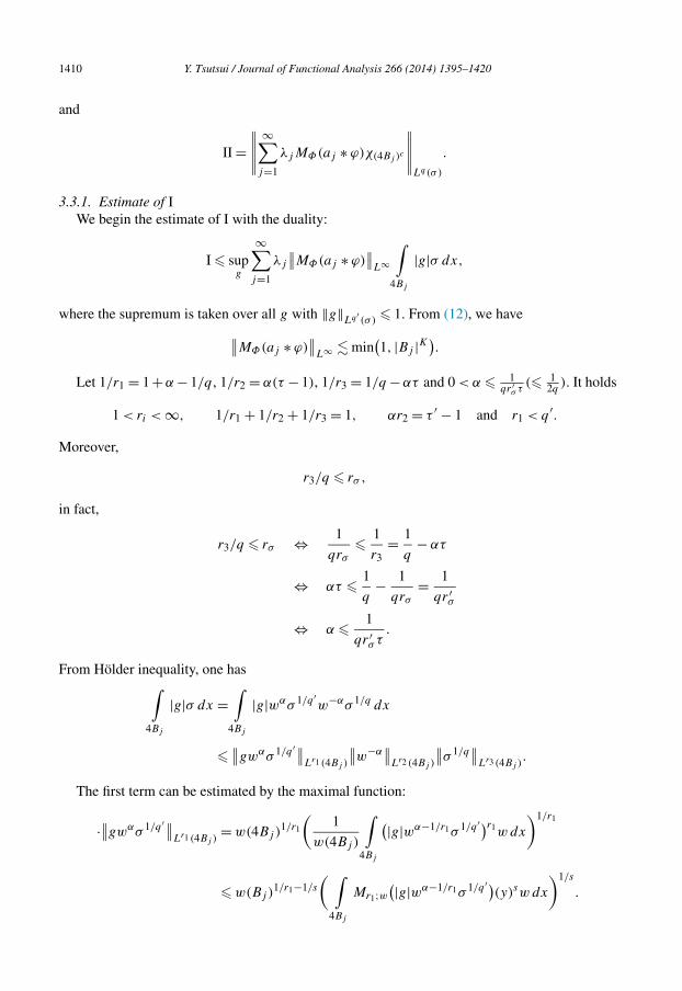
1410 Y. Tsutsui / Journal of Functional Analysis 266 (2014) 1395–1420
and
II =∥∥∥∥∥
∞∑j=1
λjMΦ(aj ∗ ϕ)χ(4Bj )c
∥∥∥∥∥Lq(σ )
.
3.3.1. Estimate of IWe begin the estimate of I with the duality:
I � supg
∞∑j=1
λj
∥∥MΦ(aj ∗ ϕ)∥∥
L∞
∫4Bj
|g|σ dx,
where the supremum is taken over all g with ‖g‖Lq′
(σ )� 1. From (12), we have∥∥MΦ(aj ∗ ϕ)
∥∥L∞ � min
(1, |Bj |K
).
Let 1/r1 = 1 +α − 1/q , 1/r2 = α(τ − 1), 1/r3 = 1/q −ατ and 0 < α � 1qr ′
σ τ(� 1
2q). It holds
1 < ri < ∞, 1/r1 + 1/r2 + 1/r3 = 1, αr2 = τ ′ − 1 and r1 < q ′.
Moreover,
r3/q � rσ ,
in fact,
r3/q � rσ ⇔ 1
qrσ� 1
r3= 1
q− ατ
⇔ ατ � 1
q− 1
qrσ= 1
qr ′σ
⇔ α � 1
qr ′σ τ
.
From Hölder inequality, one has∫4Bj
|g|σ dx =∫
4Bj
|g|wασ 1/q ′w−ασ 1/q dx
�∥∥gwασ 1/q ′∥∥
Lr1 (4Bj )
∥∥w−α∥∥
Lr2 (4Bj )
∥∥σ 1/q∥∥
Lr3 (4Bj ).
The first term can be estimated by the maximal function:
·∥∥gwασ 1/q ′∥∥Lr1 (4Bj )
= w(4Bj )1/r1
(1
w(4Bj )
∫4Bj
(|g|wα−1/r1σ 1/q ′)r1w dx
)1/r1
� w(Bj )1/r1−1/s
( ∫4B
Mr1;w(|g|wα−1/r1σ 1/q ′)
(y)sw dx
)1/s
.
j
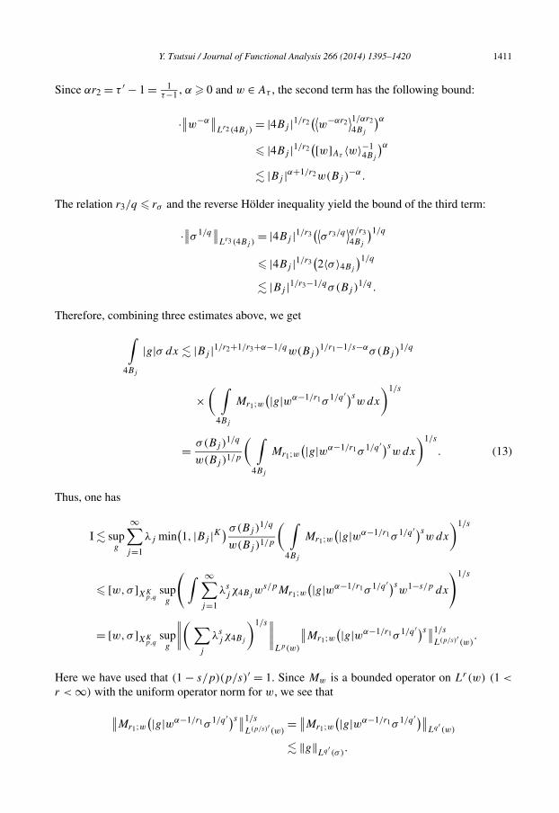
Y. Tsutsui / Journal of Functional Analysis 266 (2014) 1395–1420 1411
Since αr2 = τ ′ − 1 = 1τ−1 , α � 0 and w ∈ Aτ , the second term has the following bound:
·∥∥w−α∥∥
Lr2 (4Bj )= |4Bj |1/r2
(⟨w−αr2
⟩1/αr24Bj
)α
� |4Bj |1/r2([w]Aτ 〈w〉−1
4Bj
)α
� |Bj |α+1/r2w(Bj )−α.
The relation r3/q � rσ and the reverse Hölder inequality yield the bound of the third term:
·∥∥σ 1/q∥∥
Lr3 (4Bj )= |4Bj |1/r3
(⟨σ r3/q
⟩q/r34Bj
)1/q
� |4Bj |1/r3(2〈σ 〉4Bj
)1/q
� |Bj |1/r3−1/qσ (Bj )1/q .
Therefore, combining three estimates above, we get
∫4Bj
|g|σ dx � |Bj |1/r2+1/r3+α−1/qw(Bj )1/r1−1/s−ασ (Bj )
1/q
×( ∫
4Bj
Mr1;w(|g|wα−1/r1σ 1/q ′)s
w dx
)1/s
= σ(Bj )1/q
w(Bj )1/p
( ∫4Bj
Mr1;w(|g|wα−1/r1σ 1/q ′)s
w dx
)1/s
. (13)
Thus, one has
I � supg
∞∑j=1
λj min(1, |Bj |K
) σ(Bj )1/q
w(Bj )1/p
( ∫4Bj
Mr1;w(|g|wα−1/r1σ 1/q ′)s
w dx
)1/s
� [w,σ ]XKp,q
supg
( ∫ ∞∑j=1
λsjχ4Bj
ws/pMr1;w(|g|wα−1/r1σ 1/q ′)s
w1−s/p dx
)1/s
= [w,σ ]XKp,q
supg
∥∥∥∥( ∑
j
λsjχ4Bj
)1/s∥∥∥∥Lp(w)
∥∥Mr1;w(|g|wα−1/r1σ 1/q ′)s∥∥1/s
L(p/s)′ (w).
Here we have used that (1 − s/p)(p/s)′ = 1. Since Mw is a bounded operator on Lr(w) (1 <
r < ∞) with the uniform operator norm for w, we see that
∥∥Mr1;w(|g|wα−1/r1σ 1/q ′)s∥∥1/s
L(p/s)′ (w)= ∥∥Mr1;w
(|g|wα−1/r1σ 1/q ′)∥∥Lq′
(w)
� ‖g‖ q′ .
L (σ)
1412 Y. Tsutsui / Journal of Functional Analysis 266 (2014) 1395–1420
Here, the relations s(p/s)′ = q ′ ⇔ 1/s − 1/p = 1 − 1/q , and 1 + q ′(α − 1/r1) = 0 have beenused. Therefore, thanks to Lemma 4 in Chapter VIII in [18], we can complete the estimate of I:
I � [w,σ ]XKp,q
∥∥∥∥(∑
j
λsjχ4Bj
)1/s∥∥∥∥Lp(w)
� [w,σ ]XKp,q
‖f ‖Hp(w).
3.3.2. Estimate of IINext, we verify that
II =∥∥∥∥∥
∞∑j=1
λjMΦ(aj ∗ ϕ)χ(4Bj )c
∥∥∥∥∥Lq(σ )
has the same bound as that of I. Here, we use the same exponents r1, α and s as those in theprevious subsection. From Lemma 2.2 and (12), it follows that
MΦ(aj ∗ ϕ)(x)χ(4Bj )c (x) � min(1, |Bj |K
)( rj
|x − xj |)M
χ(4Bj )c (x),
where M = (n + N∗ + 1)/2. In fact,
MΦ(aj ∗ ϕ)(x)χ(4Bj )c (x) �∥∥MΦ(aj ∗ ϕ)
∥∥1/2L∞MΦ(aj ∗ ϕ)(x)1/2χ(4Bj )c (x)
� min(1, |Bj |K
)( rj
|x − xj |)(n+N∗+1)/2
χ(4Bj )c (x).
Hence, we obtain
II �∥∥∥∥∥
∞∑j=1
λj min(1, |Bj |K
)( rj
|x − xj |)M
χ(4Bj )c
∥∥∥∥∥Lq(σ )
= supg
∣∣∣∣∫ ∑
j
λj min(1, |Bj |K
)( rj
|x − xj |)M
χ(4Bj )cgσ dx
∣∣∣∣� sup
g
∑j
λj min(1, |Bj |K
) ∫(2Bj )c
(rj
|x − xj |)M
|g|σ dx
with the same supremum above. From (13), the last integral has the similar bound as that of I:
∫(2Bj )c
(rj
|x − xj |)M
|g|σ dx
�∑k�1
2−kM
∫2k+1B
|g|σ dx
j
Y. Tsutsui / Journal of Functional Analysis 266 (2014) 1395–1420 1413
�∑
k
2−kM σ(2k+1Bj )1/q
w(2k+1Bj )1/p
( ∫2k+3Bj
Mr1;w(|g|wα−1/r1σ 1/q ′)s
w dx
)1/s
�∑
k
(2nρ/q
2M
)k σ (Bj )1/q
w(Bj )1/p
( ∫2k+3Bj
Mr1;w(|g|wα−1/r1σ 1/q ′)s
w dx
)1/s
.
Thus, we get the desired estimate of (I) as follows:
II � [w,σ ]XKp,q
sup∑j
λj
∑k
2k(nρ/q−M)
( ∫2k+3Bj
Mr1;w(|g|wα−1/r1σ 1/q ′)s
w dx
)1/s
� [w,σ ]XKp,q
supg
∑k
2k(nρ/q−M)
×(∫ ∑
j
λsjχ2k+3Bj
ws/pMr1;w(|g|wα−1/r1σ 1/q ′)s
w1−s/p dx
)1/s
� [w,σ ]XKp,q
∑k
2k(nρ/q−M)
∥∥∥∥( ∑
j
λsjχ2k+3Bj
)1/s∥∥∥∥Lp(w)
� [w,σ ]XKp,q
∑k
2k(nρ/q+nτ/s−M)
∥∥∥∥( ∑
j
λsjχBj
)1/s∥∥∥∥Lp(w)
� [w,σ ]XKp,q
‖f ‖Hp(w).
Here we have used Lemma 4 in Chapter VIII in [18] and the relation nρ/q + nτ/s − M < 0. Asa consequence, the proof is completed. �4. Div–curl estimate for weighted Hardy spaces
In this section, we establish the weighted version of the so-called “div–curl lemma” due toCoifman, Lions, Meyer and Semmes [3].
4.1. Non-endpoint cases p < ∞
The purpose in this case is achieved by means of the pointwise estimate of bilinear form withthe cancellation property by Miyachi [15].
Proof. It is enough to show the inequality with u,∇v ∈ D0. We denote the j th Riesz trans-
form by Rj = −∂j |∇|−1 = F−1[−iξj
|ξ |F]. Since the divergence free condition of u yields thecancellation
n∑Rkuk = 0,
k=1
1414 Y. Tsutsui / Journal of Functional Analysis 266 (2014) 1395–1420
one obtains
∥∥(u · ∇)v∥∥
Hr(μ)�
n∑j,k=1
∥∥ukRk
(|∇|vj
) − (Rkuk)|∇|vj
∥∥Hr(μ)
.
It is sufficient to prove ∥∥Λ(f,g)∥∥
Hr(μ)� ‖f ‖Hp(w)‖g‖Hq(σ) (14)
with f,g ∈ D0, where Λ(f,g)(x) = ∑2λ=1(T
λ1 f )(x)(T λ
2 g)(x), T 11 h = h, T 2
1 h = −Rjh, T 12 h =
Rjh and T 22 h = h. Note that the bilinear form Λ has the moment condition∫
Λ(f,g)dx = 0,
for all f,g ∈ D0. To prove (14), we make use of the pointwise estimate for Λ due to Miyachi [15].More precisely, he showed the following: for every K ∈N∪ {0},
Λ(f,g)∗1(x) �2∑
λ=1
GK
(f,T λ
1 ,m1)(x)GK
(g,T λ
2 ,m2)(x) (15)
where GL(h,S,m)(x) = Mm(h∗L)(x)+(Sh)∗L(x), provided that 1/mj = 1/θj +sj /n and, θj and
sj satisfy the following conditions: 0 < 1/θj < 1, 1/θ1 + 1/θ2 � 1, 0 � sj < 1, s1 + s2 � 1,1/p < 1/θ1 + s1/n and 1/q < 1/θ2 + s2/n.
We check that our assumption ensures the existence of exponents (mj , θj , sj ) satisfying theseconditions.
Let m1 = p/τ ∈ (n/(n + 1),p) and m2 = q/ρ ∈ (n/(n + 1), q). Obviously, 1/p < 1/m1 <
1 + 1/n,1/q < 1/m2 < 1 + 1/n and 1/r < 1/m1 + 1/m2 < 1 + 1/n. It is possible to take θj
(j = 1,2), fulfilling the following conditions:
• 0 < 1/θ1 < 1, 1/θ1 � 1/m1 and 1/m1 − 1/n � 1/θ1 � 1 + 1/n − 1/m2,• 0 < 1/θ2 � min(1 − 1/θ1,1/m2), 1/m2 − 1/n � 1/θ2 and 1/m1 + 1/m2 − 1/θ1 − 1/n �
1/θ2.
Then, we define sj = n(1/mj − 1/θj ) (j = 1,2). From the conditions on θj above, it followsthat 0 � sj < 1 and s1 + s2 � 1. Therefore, from (15) we get
∥∥Λ(f,g)∥∥
Hr(μ)�
2∑λ=1
∥∥GK
(f,T λ
1 ,m1)∥∥
Lp(w)
∥∥GK
(g,T λ
2 ,m2)∥∥
Lq(σ ).
Because m1 < p and w ∈ Ap/m1 , it follows ‖Mm1(f∗K)‖Lp(w) � ‖f ‖Hp(w). By using Theo-
rem 14 in Chapter XI in [18], we have the boundedness of the Riesz transforms on Hp(w),which implies ∥∥(
T λj f
)∗K
∥∥Lp(w)
� ‖f ‖Hp(w).
Hence, we get the desired estimate (14). �
Y. Tsutsui / Journal of Functional Analysis 266 (2014) 1395–1420 1415
4.2. Endpoint case p = ∞
The argument above is false in the case p = ∞, because the Riesz transform Rj is an un-bounded operator on L∞. By following the argument by Auscher, Russ and Tchamitchian [1],we can show the endpoint case. For the proof of the theorem, we recall notations that wereused in [1]. For x ∈ Rn and 1 � m � ∞, let Fm(x) be a set of all vector-valued functionsΨ = (ψ1, . . . ,ψn) with ψj ∈ Lm supported in a ball B = B(xB, rB) containing x so thatthere exists a function gΨ ∈ Lm such that divΨ = gΨ in S ′, suppgΨ ⊂ B and ‖Ψ ‖Lm +rB‖gΨ ‖Lm � |B|−1/m′
. The similar one Fm(x) is defined by a set of all vector-valued func-tions Ψ = (ψ1, . . . , ψn) so that ψj ∈ W 1,m supported in a ball B = B(xB, rB) containing x
satisfying ‖Ψ ‖Lm + rB‖DΨ ‖Lm � |B|−1/m′where DΨ is the n × n matrix whose j th column
is ∇ψj . The maximal operators Nm and Nm are defined by for locally integrable functions f and{fj }nj=1
Nmf (x) = supΨ ∈Fm(x)
∫f (y)gΨ (y) dy and NmF(x) = sup
Ψ ∈Fm(x)
∫F(y) · Ψ (y) dy,
where F = (f1, . . . , fn).In the proof, we use the following basic fact:
Lemma 4.1. Let 1 < p < ∞ and w ∈ Ap . Then
∫|x|>M
w(x)
|x|np dx � M−npw(B(0,M)
).
Proof. It is sufficient to prove
∥∥∥∥∥n∑
j=1
uj∂j v
∥∥∥∥∥Hq(σ)
� ‖u‖L∞‖∇v‖Hq(σ),
for every vector-valued functions u ∈ L∞ with divu = 0 and every functions v ∈ Y with ∂j v ∈Hq(σ). Firstly, we give a definition of
∑nj=1 uj∂j v as a tempered distribution as follows: for
ϕ ∈ S
⟨n∑
j=1
uj∂j v,ϕ
⟩= −
n∑j=1
∫uj (y)v(y)∂jϕ(y) dy.
Our assumption ensures that the integrand in the right hand side is integrable. Then, it follows
n∑uj∂j v ∗ Φt(x) = −CΦ‖u‖L∞
∫v(y)
[n∑
uj (y)∂yjΦt (x − y)
]dy,
j=1 j=1
1416 Y. Tsutsui / Journal of Functional Analysis 266 (2014) 1395–1420
where CΦ is a large constant depending on n and Φ , and uj (y) = uj (y)
CΦ‖u‖L∞ . Owing to the diver-gence free condition on u, we see that for every x ∈Rn
n∑j=1
uj (y)∂yjΦt (x − y) =
n∑j=1
∂yj
(uj (y)Φt (x − y)
)in S ′(Rn
y
).
Hence, we obtain the pointwise estimate
MΦ
(n∑
j=1
uj∂j v
)(x) � CΦ‖u‖L∞Nmv(x),
for all m ∈ [1,∞]. The maximal function Nmv is pointwisely controlled by another one Nm∇v.To check this, let Ψ ∈ Fm(x) be supported in B and m ∈ (1,∞). Because the compactness of thesupport of gΨ ∈ Lm implies
∫gΨ dx = 0, from Lemma 10 in [1] there exists Ψ = (ψ1, . . . , ψn)
with ψj ∈ W 1,m(B) such that gΨ = div Ψ a.e. on Rn and ‖DΨ ‖Lm � c‖gΨ ‖Lm . The Poincaréinequality then ensures that 1
C∗ Ψ ∈ Fm(x) with some constant C∗ > 0. Therefore, we can seethat ∫
v(y)gΨ (y) dy = −∫
∇v(y) · Ψ (y) dy,
which implies that Nmv(x) � cNm∇v(x) for all x ∈ Rn. As a consequence, one obtains thepointwise estimate
MΦ
(n∑
j=1
uj∂j v
)(x) � ‖u‖L∞Nm∇v(x),
with 1 < m < ∞. Therefore, it suffices to prove that
∥∥N∗mf
∥∥Lq(σ )
� ‖f ‖Hq(σ) (16)
with some m ∈ (1,∞), where N∗mf (x) = supψ∈Λm(x) |
∫f (y)ψ(y)dy| and Λm(x) is a space
of all functions ψ ∈ W 1,m supported in a ball B = B(xB, rB) containing x satisfying ‖ψ‖Lm +rB‖∇ψ‖Lm � |B|−1/m′
.Let f = ∑∞
j=1 λjaj be an atomic decomposition from Theorem A when q � 1 or Theorem Cwhen q > 1.
We shall show the inequality (16) in the case 0 < q � 1. From the openness property ofMuckenhoupt classes, there exists m > n so that σ ∈ Aq(1/m′+1/n). Because
∥∥N∗mf
∥∥Lq(σ )
�( ∞∑
j=1
|λj |q∥∥N∗
maj
∥∥q
Lq(σ )
)1/q
,
it is sufficient to show that supj ‖N∗maj‖Lq(σ ) � 1. To do so, let a be an atom, i.e. suppa ⊂
B0 = B(x0, r0), ‖a‖L∞ � σ(B0)−1/q and
∫xαa(x) dx = 0 for all |α| � 1. Fix x ∈ Rn and take
Y. Tsutsui / Journal of Functional Analysis 266 (2014) 1395–1420 1417
ψ ∈ Λm(x) supported in B = B(x, r). Since | ∫ a(y)ψ(y)dy| � ‖a‖L∞‖ψ‖L1 � σ(B0)−1/q , we
see that
∥∥(N∗
ma)χ4B0
∥∥Lq(σ )
� 1.
Consider the case x /∈ 4B0. In this case, if cr < |x − x0| with c > 12/7, then∫
aψ dy = 0. Onthe other hand, in the case |x − x0| � cr , the same calculus as that in pp. 74–75 in [1] yields
∣∣∣∣∫
a(y)ψ(y)dy
∣∣∣∣ �(
r0
|x − x0|)1+n/m′
σ(B0)−1/q .
Here we have used that m > n. Hence, by using Lemma 4.1, one obtains ‖(N∗ma)χ(4B0)
c‖Lq(σ ) �1, which completes the proof in this case.
To give a proof in the case q ∈ (1,∞), let a be an atom, i.e. suppa ⊂ B0, ‖a‖L∞ � 1 and∫xαa(x) dx = 0 for all |α| � 1. Obviously, ‖N∗
ma‖L∞ � 1. For x �∈ 4B0, it can be seen thatN∗
ma(x) has the same bound as that in the previous case without σ(B0)−1/q . From the argument
in Subsection 3.3, these estimates imply (16) with large m. Remark that this discussion can workunder the assumption σ ∈ A∞. The proof is completed. �5. Application to the decay property of solutions to Navier–Stokes equations
In this final section, we prove Theorem 1.4 by using theorems that are established in theprevious sections.
Proof of Theorem 1.4. The openness property of Muckenhoupt classes, see Remark 1.1, ensuresthe existence of N ∈ (1, q(1 + 1/n)) such that σ ∈ AN . From our assumption, we can takeτ, θ ∈ (n,∞) fulfilling
α < n(1 + 1/n − 1/p − 1/τ), N < q(1 + 1/n − 1/τ) and 1/n − 1/τ < 1/θ < 1/n.
Let 1/r = 1/p + 1/τ . Then, we define
‖u‖X = supt>0
∥∥u(t)∥∥
Ln + supt>0
t1/2∥∥u(t)
∥∥L∞ + sup
t>0t1−n/(2τ)
∥∥∇u(t)∥∥
Lτ
= ‖u‖X1 + ‖u‖X2 + ‖u‖X3,
‖u‖Y = supt>0
∥∥u(t)∥∥
Hp(w)+ sup
t>0tn(1/p−1/q)/2+(α−β)/2
∥∥u(t)∥∥
Hq(σ)+ sup
t>0t1/2
∥∥∇u(t)∥∥
Hp(w)
= ‖u‖Y1 + ‖u‖Y2 + ‖u‖Y3,
and let X be a Banach space of all divergence free vector functions u satisfying ‖u‖X < ∞ andlimt↘0(t
1/2‖u(t)‖L∞ + t1−n/(2τ)‖∇u(t)‖Lτ ) = 0, and Y = {u; ‖u‖Y < ∞, divu = 0}. Let
‖h‖Xθ= sup
t>0tn(1/n−1/θ)/2
∥∥h(t)∥∥
Lθ � ‖h‖n/θX1
‖h‖1−n/θX2
.
We construct solutions in X ∩ Y through Picard’s iteration scheme.
1418 Y. Tsutsui / Journal of Functional Analysis 266 (2014) 1395–1420
Step 1. It is not hard to see that ‖u0‖X � cδ and
limt↘0
t1/2∥∥et�a
∥∥L∞ = lim
t↘0t1−n/(2τ)
∥∥∇et�a∥∥
Lτ = 0
by density. Moreover, Theorem 1.1 gives ‖u0‖Y1 � cδ.
Step 2. ‖B(f,g)‖X � c‖f ‖X‖g‖X can be seen from the following estimates:
·∥∥B(f,g)(t)∥∥
Ln �t∫
0
(t − s)−(n/θ−1)/2∥∥f (s)
∥∥Ln‖g‖Lθ ds
� ‖f ‖X1‖g‖Xθ,
·∥∥B(f,g)(t)∥∥
L∞ �t∫
0
(t − s)−n/(2θ)∥∥f (s)
∥∥Lθ
∥∥∇g(s)∥∥
Lτ ds
� t−1/2‖f ‖Xθ‖g‖X3,
·∥∥∇B(f,g)(t)∥∥
Lτ �t∫
0
(t − s)−(n/θ+1)/2∥∥f (s)
∥∥Lθ
∥∥∇g(s)∥∥
Lτ ds
� t−1+n/(2τ)‖f ‖Xθ‖g‖X3 .
These estimates also imply that B(f,g) ∈ X and limt↘0 ‖B(f,g)(t)‖Ln = 0 whenever f and g
belong to X. By using Corollary 1.1 and Theorem 1.2, one obtains
∥∥B(f,g)(t)∥∥
Hp(w)� c
t∫0
(t − s)−n(1/p+1/τ−1/p)/2∥∥(f · ∇)g(s)
∥∥Hr(|·|αr )
ds
� c
t∫0
(t − s)−n/(2τ)s−(1−n/(2τ)) ds ‖f ‖Y1‖g‖X3
� c‖f ‖Y1‖g‖X3 . (17)
On one hand, we have
∥∥e(t−s)�P(f · ∇)g(s)∥∥
Hq(σ)� (t − s)−n(1/r−1/q)/2−(α−β)/2
∥∥(f · ∇)g(s)∥∥
Hr(|·|rα)
� (t − s)−n(1/p+1/τ−1/q)/2−(α−β)/2∥∥f (s)
∥∥Hp(w)
∥∥∇g(s)∥∥
Lτ
� (t − s)−n(1/p+1/τ−1/q)/2−(α−β)/2s−(1−n/(2τ))‖f ‖Y1‖g‖X3 .
On the other hand, it follows that with 1/r = 1/q + 1/τ
Y. Tsutsui / Journal of Functional Analysis 266 (2014) 1395–1420 1419
∥∥e(t−s)�P(f · ∇)g(s)∥∥
Hq(σ)� (t − s)−n(1/r−1/q)/2
∥∥(f · ∇)g(s)∥∥
Hr(|·|βr
)� (t − s)−n/(2τ)
∥∥f (s)∥∥
Hq(σ)
∥∥∇g(s)∥∥
Lτ
� (t − s)−n/(2τ)s−n(1/p−1/q)/2−(α−β)/2−(1−n/(2τ))‖f ‖Y2‖g‖X3 .
Combining these estimates, it holds that
∥∥B(f,g)∥∥
Y2� c
(‖f ‖Y1 + ‖f ‖Y2
)‖g‖X3 . (18)
Further, ‖B(f,g)‖Y3 � c‖f ‖Y1‖g‖X3 can be found from
∥∥∇e(t−s)�P(f · ∇)g(s)∥∥
Hp(w)� (t − s)−1/2−n/(2τ)s−(1−n/(2τ))‖f ‖Y1‖g‖X3 .
As a consequence, we can find a global solution u ∈ X∩Y with ‖u‖X +‖u‖Y � cδ and u(t) → a
in Ln as t tends to 0. It is not hard to see that u ∈ C([0,∞);Ln). Furthermore, from Proposi-tion 15.1 in [12], we see u ∈ C∞((0,∞) ×Rn).
Step 3. We shall show that u ∈ C([0,∞);Hp(w)). From (ii) of Remark 4.5 in [2], we can seethat ‖et�a − a‖Hp(w) → 0 as t tends to 0. (17) implies the convergence ‖B(u,u)(t)‖Hp(w) → 0as t tends to 0. The continuity of the linear part et�a in Hp(w) can be proved by Theorem 1.1.From 2 of Remark 1.3, we have
∥∥et�a − es�a∥∥
Hp(w)� |G√
t − G√s |S‖a‖Hp(w) → 0 as |t − s| → 0.
To check the continuity of the non-linear part B(u,u), we consider that for t+ > t−
B(u,u)(t+) − B(u,u)(t−)
=t−∫
0
e(t+−s)�P(u · ∇)u(s) − e(t−−s)�P(u · ∇)u(s) ds +t+∫
t−
e(t+−s)�P(u · ∇)u(s) ds.
From Theorem 1.3, we have the uniform bound for t
∥∥e(t−s)�P(u · ∇)u(s)∥∥
Hp(w)�
∥∥u(s)∥∥
L∞∥∥∇u(s)
∥∥Hp(w)
. (19)
The continuity of the heat semigroup on weighted Hardy spaces, proved by Bui [2], ensuresthat the first term goes to 0 as |t+ − t−| ↘ 0. Remark that P(u · ∇)u ∈ Hr(| · |αr ). The uniformestimate (19) implies that the second term tends to 0 as |t+ − t−| ↘ 0.
Step 4. Finally, we check (4). In the case p < q or β < α, from the density of D0 in Hp(w), itholds that
limt↘0
tn(1/p−1/q)/2+(α−β)/2∥∥et�a
∥∥Hq(σ)
= 0.
This and the bilinear estimate (18) yield (4). �
1420 Y. Tsutsui / Journal of Functional Analysis 266 (2014) 1395–1420
Acknowledgments
The author would like to thank Professor Hideo Kozono for suggesting the problem and valu-able comments. The author is grateful to Professor Akihiko Miyachi for fruitful suggestions andProfessors Yoshihiro Sawano and Hitoshi Tanaka and Doctor Xiao Lian for valuable discussionand pointing out some typos. The author would like to thank the referee for carefully reading.This work was supported by Grant-in-Aid for JSPS Fellows.
References
[1] P. Auscher, E. Russ, P. Tchamitchian, Hardy Sobolev spaces on strongly Lipschitz domains of Rn, J. Funct. Anal.218 (1) (2005) 54–109.
[2] H.Q. Bui, Weighted Besov and Triebel spaces: interpolation by the real method, Hiroshima Math. J. 12 (3) (1982)581–605.
[3] R. Coifman, P.L. Lions, Y. Meyer, S. Semmes, Compensated compactness and Hardy spaces, J. Math. Pures Appl.72 (1993) 247–286.
[4] C. Fefferman, E. Stein, Hp spaces of several variables, Acta Math. 129 (1972) 137–193.[5] J. García-Cuerva, Weighted Hp-spaces, Disertationes Math. 162 (1979).[6] A.E. Gatto, C.E. Gutiérrez, R.L. Wheeden, Fractional integrals on weighted Hp spaces, Trans. Amer. Math. Soc.
289 (2) (1985) 575–589.[7] Y. Giga, T. Miyakawa, Solutions in Lr of the Navier–Stokes initial value problem, Arch. Ration. Mech. Anal. 89 (3)
(1985) 267–281.[8] L. Grafakos, Modern Fourier Analysis, second ed., Grad. Texts in Math., vol. 250, Springer-Verlag, 2008.[9] T. Hytönen, C. Pérez, Sharp weighted bounds involving A∞ , Anal. PDE 6 (4) (2013) 777–818.
[10] T. Kato, Strong Lp-solutions of the Navier–Stokes equation in Rn, with applications to weak solutions, Math. Z.187 (1984) 471–480.
[11] M.-Y. Lee, C.-C. Lin, The molecule characterization of weighted Hardy spaces, J. Funct. Anal. 188 (2002) 442–460.[12] P.G. Lemarié-Rieusset, Recent Development in the Navier–Stokes Problem, Chapman & Hall/CRC Res. Notes
Math., vol. 431, Chapman & Hall/CRC, Boca Raton, FL, 2002.[13] A.K. Lerner, S. Ombrosi, C. Pérez, Sharp A1 bounds for Calderón–Zygmund operators and the relationship with a
problem of Muckenhoupt–Wheeden, Int. Math. Res. Not. 2008 (2008), 11 pp.[14] A. Miyachi, Weighted Hardy spaces on a domain, in: Proceedings of the Second ISAAC Congress, vol. 1, Fukuoka,
1999, in: Int. Soc. Anal. Appl. Comput., vol. 7, Kluwer Acad. Publ., Dordrecht, 2000, pp. 59–64.[15] A. Miyachi, Hardy space estimate for the product of singular integrals, Canad. J. Math. 52 (2) (2000) 381–411.[16] T. Miyakawa, Hardy spaces of solenoidal vector fields, with applications to the Navier–Stokes equations, Kyushu
J. Math. 50 (1) (1996) 1–64.[17] T. Miyakawa, Application of Hardy space techniques to the time-decay problem for incompressible Navier–Stokes
flows in Rn, Funkcial. Ekvac. 41 (3) (1998) 383–434.[18] J.-O. Strömberg, A. Torchinsky, Weighted Hardy Spaces, Lecture Notes in Math., vol. 1381, Springer-Verlag, Berlin,
1989.[19] M.H. Taibleson, G. Weiss, The Molecular Characterization of Certain Hardy Spaces. Representation Theorems for
Hardy Spaces, Astérisque, vol. 77, Soc. Math. France, Paris, 1980, pp. 67–149.[20] Y. Tsutsui, The Navier–Stokes equations and weak Herz spaces, Adv. Differential Equations 16 (11–12) (2011)
1049–1085.[21] M. Wiegner, Decay results for weak solutions of the Navier–Stokes equations on Rn, J. London Math. Soc. (2)
35 (2) (1987) 303–313.