AN APPLICATION OF SURVIVAL ANALYSIS ON THE PREVALENCE …

AN APPLICATION OF SURVIVAL ANALYSIS ON THE PREVALENCE

AND RISK FACTORS OF BREAST CANCER IN NAMIBIA

A MINI THESIS SUBMITTED IN PARTIAL FULFILMENT OF THE REQUIREMENTS

FOR THE DEGREE

OF

MASTER OF SCIENCE IN BIOSTATISTICS

OF

THE UNIVERSITY OF NAMIBIA

BY

ALEXANDRINA PETRUS

201204368

APRIL 2019

SUPERVISOR: DR OPEOLUWA OYEDELE (DEPARTMENT OF STATISTICS AND

POPULATION STUDIES – UNAM)

i

ABSTRACT

Cancer is a universal disease that affects people regardless of race, sex, socio-economic status and

culture. With just an approximated population size of 2.3 million people NSA (2011), Namibia is

not excluded from this. If not detected on time and treated on time, cancer can make treatment less

likely to succeed and reduce the chances of survival.

The study was aimed at examining the prevalence and trends for breast cancer patients, regardless

of patients’ sex, as well as establishing the risk factors associated with breast cancer in Namibia.

Secondary data obtained from the Cancer Association of Namibia for the periods of 2013 to 2016

was used. Descriptive statistics were performed in the form of figures and tables to explore

demographic characteristics of the patients. Survival analysis techniques (Kaplan-Meier to

construct the survival curves, Log-Rank Test to determine differences in survival between groups

and Cox Proportional Hazard to investigate the association between the survival time of the

patients and their demographic characteristics) were used to estimate the survival rate of the breast

cancer patients. Patient survival was measured by their age at diagnosis and their age at death.

Thus, the event variable was the patient’s status (alive or dead). Results revealed that breast cancer

can affect anybody regardless of sex in Namibia. Khomas and Oshana regions had the highest

percentage of reported breast cancers cases. Results showed that the survival rate of breast cancer

was influenced by Age group, and Ethnicity. Vambos were the most diagnosed with breast cancer

followed by Whites. Factors that were significantly associated with breast cancer were age

category of 41-50 and 61-70 years. The older the patient becomes the more likely they were to

experience an event, because the Hazard Ratio had been increasing with age. The research

concluded that Age, Ethnicity and Date of diagnosis were associated with breast cancer in

Namibia. The research study recommends that there is a need of a greater focus along the breast

cancer care pathway in Namibia, with emphases on improving access to early diagnosis at early

age.

Keywords: Breast cancer, Kaplan Meier, Cox Proportional Hazard

ii

TABLE OF CONTENTS

ABSTRACT .................................................................................................................................................. i

LIST OF TABLES ..................................................................................................................................... iv

LIST OF FIGURES .................................................................................................................................... v

LIST OF ABBREVIATIONS / ACRONYMS ......................................................................................... vi

ACKNOWLEDGEMENT ........................................................................................................................ vii

DEDICATION.......................................................................................................................................... viii

DECLARATIONS ..................................................................................................................................... ix

CHAPTER 1: INTRODUCTION .............................................................................................................. 1

1.1 Background of the study ............................................................................................................... 1

1.2 Statement of the problem .............................................................................................................. 3

1.3 Objectives of the study .................................................................................................................. 4

1.4 Significance of the study ............................................................................................................... 4

1.5 Limitation of the study .................................................................................................................. 4

1.6 Delimitation of the study............................................................................................................... 5

CHAPTER 2: LITERATURE REVIEW .................................................................................................. 6

2.1 Introduction ......................................................................................................................................... 6

2.2 Breast Cancer review .......................................................................................................................... 6

2.3 Factors on breast cancer review ........................................................................................................ 10

2.4 Survival analysis review ................................................................................................................... 11

2.5 Kaplan Meier review ......................................................................................................................... 12

2.6 Cox Proportional Hazard review ....................................................................................................... 13

2.7 Literature summary ........................................................................................................................... 14

CHAPTER 3: RESEARCH METHODS ................................................................................................ 16

iii

3.1 Introduction ................................................................................................................................. 16

3.2 Research Design .......................................................................................................................... 16

3.3 Population ................................................................................................................................... 16

3.4 Sample......................................................................................................................................... 17

3.5 Procedure .................................................................................................................................... 17

3.6 Data analysis ............................................................................................................................... 20

3.6.1 Survival analysis ................................................................................................................. 21

3.6.2 Kaplan Meier ...................................................................................................................... 22

3.6.3 Confidence Interval for Kaplan Meier ................................................................................ 24

3.6.4 Log-Rank Test..................................................................................................................... 25

3.6.5 Cox Proportional Hazard .................................................................................................... 26

3.6.6 Research ethics .................................................................................................................... 28

CHAPTER 4: DATA ANALYSIS ........................................................................................................... 29

4.1 Introduction ....................................................................................................................................... 29

4.2 Descriptive statistics ................................................................................................................... 29

4.3 Survival Analysis ........................................................................................................................ 37

4.3.1 Kaplan Meier (KM .............................................................................................................. 37

4.3.2 Testing of Proportional Hazard assumptions ...................................................................... 51

4.3.3 Cox Proportional Hazard model ......................................................................................... 53

CHAPTER 5: GENERAL DISCUSSION, CONCLUSION AND RECOMMENDATIONS ............ 56

5.1 INTRODUCTION ..................................................................................................................... 56

5.2 GENERAL DISCUSSION ....................................................................................................... 56

5.3 CONCLUSION ......................................................................................................................... 57

5.4 RECOMMENDATIONS .......................................................................................................... 58

REFERENCES .......................................................................................................................................... 59

APPENDICES ........................................................................................................................................... 62

R – Codes ................................................................................................................................................ 62

iv

LIST OF TABLES

Table 1: Description of key variables ........................................................................................... 18

Table 2: Reported breast cancer case across sex from 2013-2016 ............................................... 30

Table 3: Number of reported breast cancer cases in regions Namibia from 2013-2016 .............. 31

Table 4: Reported breast cancer cases across age group from 2013-2016 ................................... 32

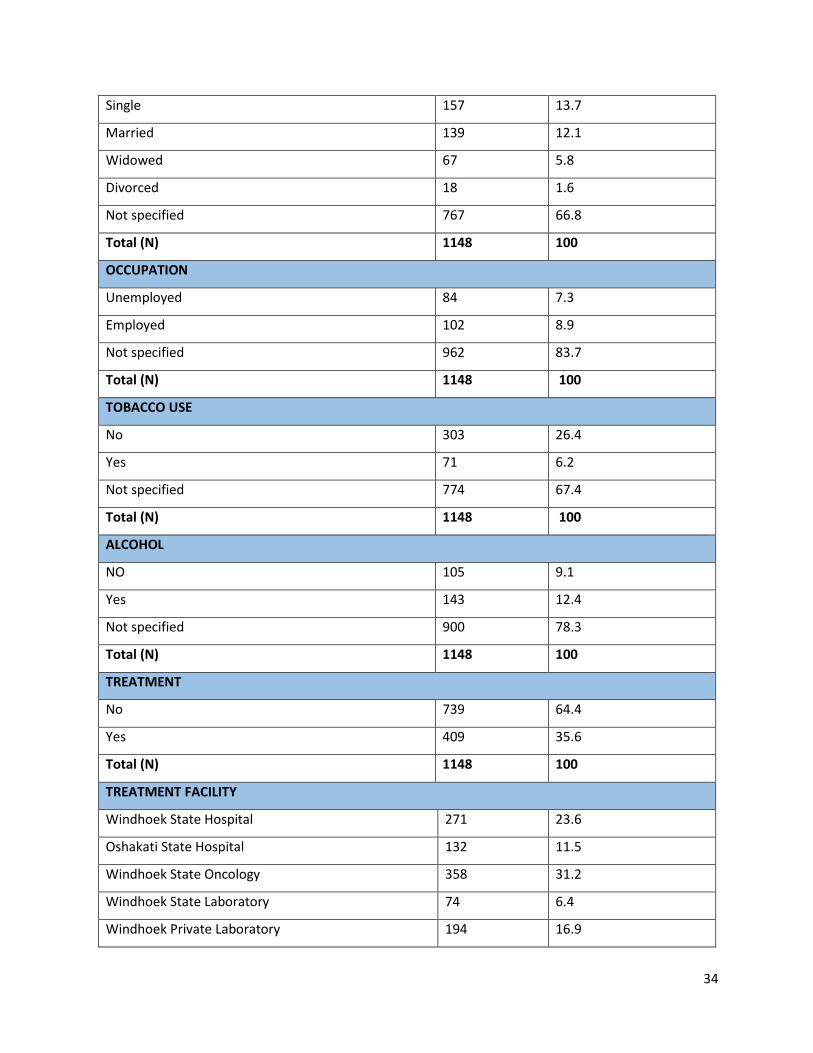
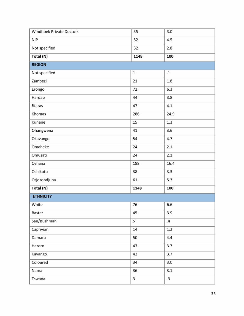
Table 5: Socio- demographic information of the breast cancer patients ...................................... 33

Table 6: Summaries of quantiles of corresponding confidence limits output .............................. 38

Table 7: Log Rank (Mantel- Cox) test of equality of survival distributions ................................ 39

Table 8: Output of Proportional Hazard assumptions ................................................................... 51

Table 9: Output from the fitted CPH regression model for 2013-2016 breast cancer patient

survival .......................................................................................................................................... 53

v

LIST OF FIGURES

Figure 1: Warning signs of Breast Cancer ...................................................................................... 1

Figure 2: Breast cancer cases reported in Namibia for 2013-2016 ............................................... 29

Figure 3: Percentage of breast cancer cases reported across the sexes from 2013-2016 .............. 31

Figure 4: Kaplan Meier curve for sex ........................................................................................... 40

Figure 5: Kaplan Meier curve for age group ................................................................................ 41

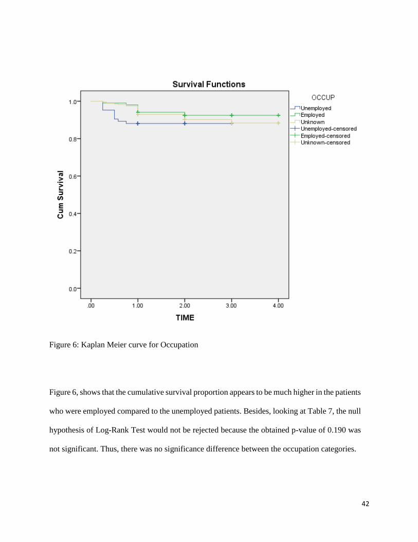
Figure 6: Kaplan Meier curve for Occupation .............................................................................. 42

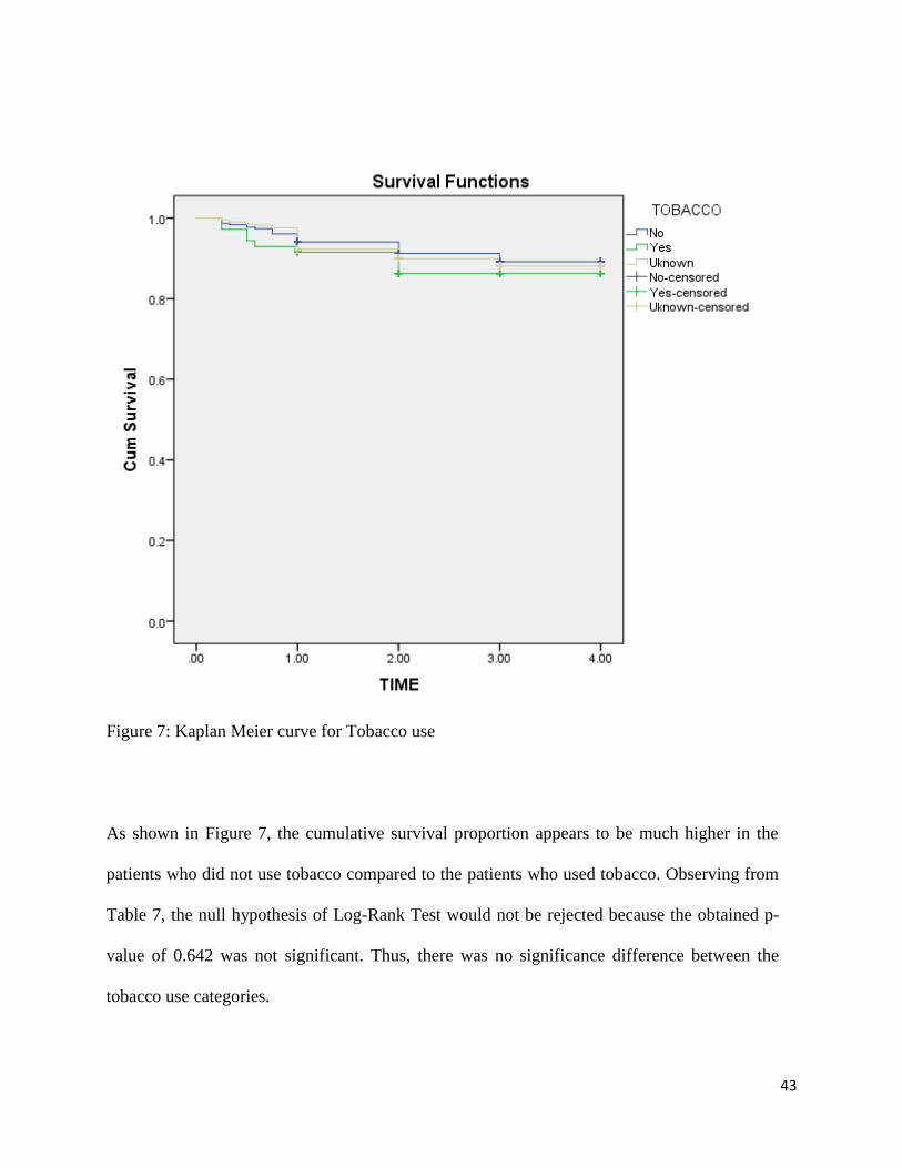
Figure 7: Kaplan Meier curve for Tobacco use ............................................................................ 43

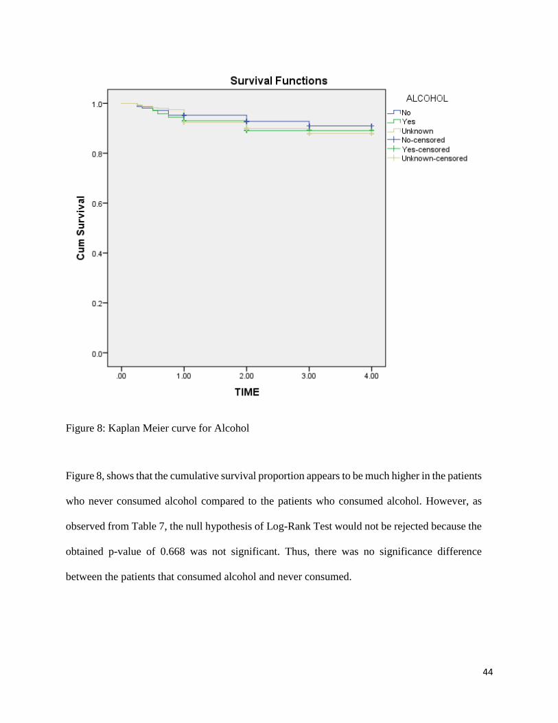
Figure 8: Kaplan Meier curve for Alcohol ................................................................................... 44

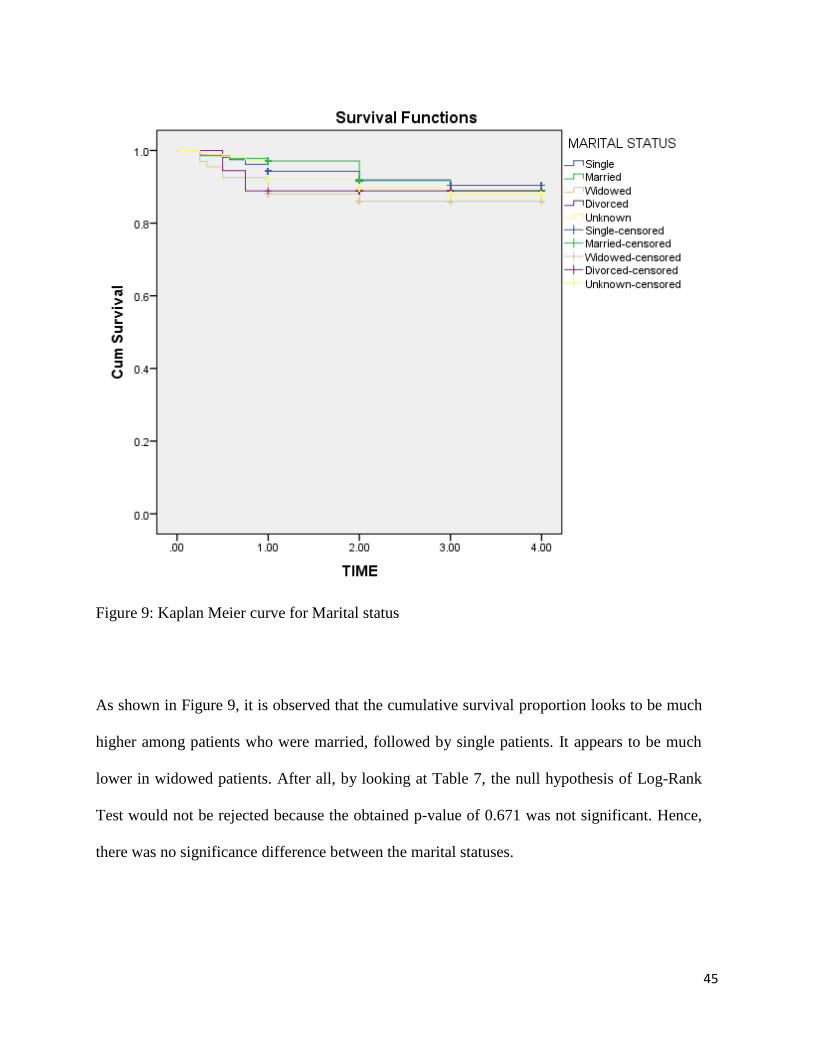
Figure 9: Kaplan Meier curve for Marital status .......................................................................... 45

Figure 10: Kaplan Meier curve for Ethnicity ................................................................................ 46

Figure 11: Kaplan Meier curve for Regions ................................................................................. 47

Figure 12: Kaplan Meier curve for Treatment .............................................................................. 48

Figure 13: Kaplan Meier curve for treatment facility ................................................................... 49

Figure 14: Kaplan Meier curve for date of diagnosis ................................................................... 50

vi

LIST OF ABBREVIATIONS / ACRONYMS

CAN Cancer Association of Namibia

CI Confidence Interval

CPH Cox Proportional Hazard

HIC High Income Countries

HR Hazard Ratio

KM Kaplan Meier

LR Log Rank

NIP Namibia Institute of Pathology

NNCR Namibia National Cancer Registry

NSA Namibia Statistics Agency

PH Proportional Hazard

PLI Product Limit

SA South Africa

SANCR South Africa National Cancer Registry

SDG Sustainable Development Goals

SPSS Statistical Package for the Social Science

WHO World Health Organization

vii

ACKNOWLEDGEMENT

In the first place I would like to appreciate almighty God, because with God everything is possible

and can be achieved.

I would like to express my sincere gratitude to the University of Namibia, especially the

department of statistics and population studies for letting me to achieve my dream of being a

masters degree holder in biostatistics.

In addition, I am gratefully indebted to my supervisor Dr. Opeoluwa Oyedele for her valuable

comments throughout this research work. Her door was always open whenever I was faced with

difficulties during my research work. She consistently allowed this research work to be my own,

but steered me in the right direction each time I needed it.

I would also like to thank the Cancer Association of Namibia (CAN) for availing their data for my

research work and the UNAM Postgraduate committee for approving my research topic and all

experts who were involved in the validation for this research project. Without their passionate

participation and input, this research study could not have been successfully executed.

Lastly I thanked all my lecturers, relatives (Maria Shahonya and Natalia Ndaitwa), classmates

(Haufiku Adolf, Andreas Shipanga, Jason Nakaluudhe, Job Shikongo, and Simon Kashihalwa),

my friends Elizabeth Elago, Delila Mutota, Randy Boois, Eunike Mwatanhele and Hendrina

Hamata, and my colleague Veronika Mukubonda for their assistance, suggestions and words of

encouragement through the journey of this research work.

viii

DEDICATION

This mini – Thesis is dedicated to Emilia Ndalinoshisho Knowledge (my first daughter), Etuna

Tuyenikumwe Wisdom (my last born) and Meekulu Maria, (my precious grandmother).

ix

DECLARATIONS

I, Alexandrina Petrus, hereby declare that this study is my own work and is a true reflection of my

research, and that this work, or any part thereof has not been submitted for a degree at any other

institution.

No part of this thesis may be reproduced, stored in any retrieval system, or transmitted in any

form, or by means (e.g. electronic, mechanical, photocopying, recording or otherwise) without the

prior permission of the author, or the University of Namibia in that behalf.

I, Alexandrina Petrus, grant the University of Namibia the right to reproduce this thesis in whole

or in part, in any manner or format, which the University of Namibia may deem fit.

……………………………. ………………….. ………….....

Name of the student Signature Date

1

CHAPTER 1: INTRODUCTION

1.1 Background of the study

As per Hejmadi (2010) cancer can be defined as a disease in which a group of abnormal cells grow

uncontrollably by disregarding the normal rules of cell division. Its growth can develop in any

parts of the human body and the most common parts are breasts, colon, lungs and prostate. The

fear of this disease is very strong that a person may delay examinations and diagnosis hoping that

the signs and symptoms will disappear. The lapse of time between awareness of a problem and

seeking medical attention can also affect the impact of diagnosis and treatment of cancer (Young,

van Niekerk & Mogotlane, 2003, as cited by Iita, 2009). If cancer is not detected on time and

treated on time, it can make treatment less likely to succeed and reduces the chances of survival.

Cancer is a universal disease that affects people regardless of race, sex, socio-economic status and

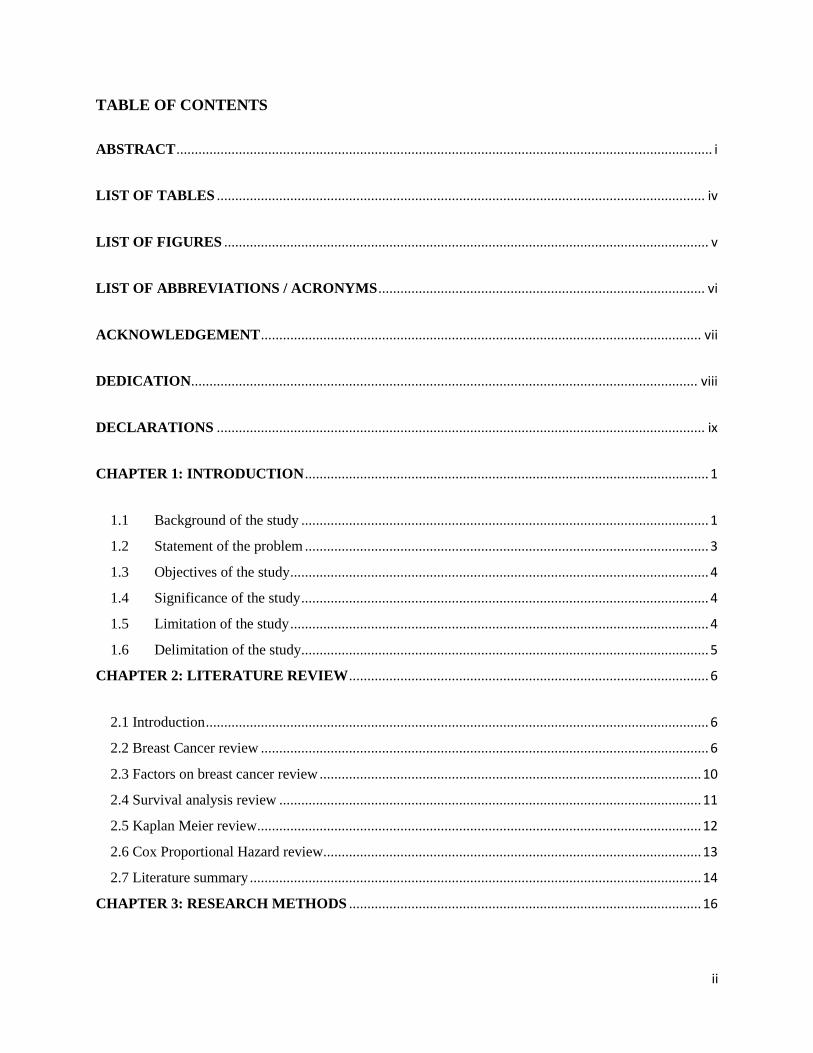
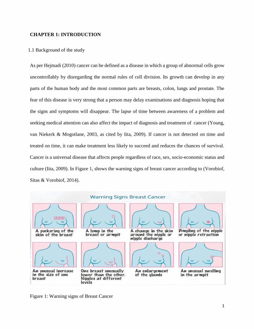
culture (Iita, 2009). In Figure 1, shows the warning signs of breast cancer according to (Vorobiof,

Sitas & Vorobiof, 2014).

Figure 1: Warning signs of Breast Cancer

2

According to the report of WHO (2014), Cancer is a leading cause of disease worldwide. An

estimated 14.1 million new cancer cases occurred in 2012. Lung, female breast, colorectal and

stomach cancers accounted for more than 40% of all cases diagnosed worldwide. In men, lung

cancer was the most common cancer (16.7% of all new cases in men). Breast cancer was by far

the most common cancer diagnosed in women (25.2% of all new cases in women).

According to South Africa’s National Cancer Registry, breast cancer was the most commonly

diagnosed cancer among women in 2011, with an age-adjusted incidence rate of 31.4 per 100 000

women and a lifetime risk of 1 in 29. In 2012, 9 815 women were diagnosed with breast cancer,

and 3 848 died from the disease. The Sustainable Development Goals (SDGs), to which South

Africa is committed, call for universal access to reproductive health services and one-third

reduction in premature deaths caused by non-communicable diseases, including cancer, by 2030.

However, without significant shifts in the funding and advocacy for women’s cancers, these goals

may go unmet in South Africa and elsewhere (Lince-Deroche et al., 2017). However they

mentioned that little has been written about breast-cancer services in South Africa and

recommendend to establish strong monitoring and evaluation systems to track access to and

utilisation of screening, diagnostic and treatment services nationwide.

The Namib Time’s (2013) research “In Namibia alone the numbers are high marking breast cancer

the third most worrisome type of cancer. Statistics surrounding new cases of breast cancer are as

follows: In 2008, there were 253 women and 7 men who had breast cancer, in 2009 there were 278

women and 6 men who developed breast cancer, in 2010 there were 288 cases in total, and in 2011

there were 291 new cases in women and 5 new cases in men. With these numbers continuously

increasing, awareness in education and research are of utmost importance” (Mowa 2016 pp.3). In

3

the mean time Carrara (2017) indicated that, the breast cancer proportion is 27.4% of all cancers

in women followed by cervix cancer with 19.4%. Pazvakawambwa & Embula, (2017) did a study

about survival analysis in Namibia to establish the prevalence, trends and risk factors for Breast

Cancer in Namibia from 2000 to 2015.

1.2 Statement of the problem

According to a study done by Mowa (2016) since 2006 cancer cases increased in Namibia with a

total of 1625, then compared to 3092 cases recorded in 2012, where 229 in 2006 and 458 in 2012

are breast cancers regardless of gender. In a report by Carrara (2017), breast cancer in the year 2010

to 2014 was recorded as being the most cancer diagnosed among Namibian women, totaling at

1579 cases. Carrara (2017) further indicated that annual incidence has increased with older age

group, escalating at 189.1 per 100 000 in women in the 70-74 years of age. This literally means

that, the number of breast cancer incidences in Namibia is increasing despite the numerous cancer

awareness and prevention programmes setups in the country. Also the burden of cancer is

increasing economically in developing countries like Namibia as a result of cancer mortality,

although it is difficult to accurately determinine the exact value of cancer burden mortality in these

countries. For these reasons, this study aims to examine the prevalence as well as risk factors

assosiated with breast cancer in Namibia.

4

1.3 Objectives of the study

The main objective of this study is to establish the risk factors associated with breast cancer in

Namibia. This will be accomplished by addressing the following sub-objectives:

a) examining the prevalence and trends for breast cancer patients in Namibia, regardless of

their sex;

b) Fitting an event history model to breast cancer data in Namibia

c) Identifying the risk factors for breast cancer in Namibia.

1.4 Significance of the study

The results from this study can be used to further guide ordinary men and women as well as policy

makers to be knowledgeable about the risk factors associated with breast cancer in Namibia, besides

the popularly known factors such as smoking and physical inactivity. Moreover, the estimated

survival time of breast cancer patients, taking into account the identified risk factors highlighted in

this study can help to contribute to a better health service planning in Namibia. All in all, the

findings from the study would add value to the body of scientific knowledge on breast cancer in

Namibia and globally.

1.5 Limitation of the study

This study will make use of the available data from the Cancer Association of Namibia (CAN) from

2013 - 2016. The limitation of this study is data because patients’ records are manually recorded at

the hospitals and sometimes not adequately captured. In addition, due to the study data being a

5

secondary data, the occurrence of missing data is highly possible. This may be attributed to some

patients not returning to the hospitals where their information was initially captured due to several

reasons such as migration and lack of transportation among others.

1.6 Delimitation of the study

The study will focus on patients diagnosed with breast cancer in Namibia from 2013 to 2016.

However, these may not necessarily reflect the true and current cancer statistics for 2018 in Namibia

6

CHAPTER 2: LITERATURE REVIEW

2.1 Introduction

This literature review gave an overview of the studies done about breast cancer in Namibia, South

Africa, and African continent at large as well as other countries at different continents, such as

Brazil and New Zealand. This chapter presented as well, how survival methods were applied in

other studies such as Kaplan Meier, Log-Rank test and Cox Proportional Hazard. In addition, it

pointed out the importance of using survival techniques on breast cancer studies.

2.2 Breast Cancer review

There is limited information about the challenges of cancer management and attempts at improving

outcomes in Africa. Publication on breast cancer in Africa start by describing a large number of

patients presenting with advanced disease, limited access to cancer education, screening, and care

(Vanderpuye et al., 2017). As it is learned from the previous studies (Iita, 2009 and Lince-Deroche

et al., 2017) that registries are still missing and if exist the quality of the data is poor in Africa or

are only hospital based in most regions of the continent. The estimates of breast cancer incidence

are presented as figures but not with the real data as the current situation, remains still to be

determined (Vanderpuye et al., 2017). This journal report by Vanderpuye et al. continues

informing that Cancer mortality rates in African countries are not comparable to those of High-

Income Countries (HIC), reaching unacceptable high proportions. The Concorde −2 study of 5-

year breast cancer survival from 1995 to 2009 based on the analysis of individual data from 279

population-based registries in 67 countries, reported that, in HIC, age-standardized net survival

rates were more than 85% (Vanderpuye et al., 2017). One country in Africa, Mauritius, a HIC

7

island nation off the coast of Madagascar, had similar survival rates of 87.4% (95% CI: 78.1–96.7).

North African countries had lower outcomes compared to HIC, for example, 59.8% (95% CI:

48.6–71.1) in Algeria, 76.6% (95% CI: 55.5–97.7) in Libya (Benghazi registry) and 68.4% (95%

CI: 64.5–72.2) in Tunisia. By contrast, data available from three Sub-Saharan countries, South

Africa 53.4% (95% CI: 35.5–71.3), The Gambia 11.9 % (95% CI: 0–24.7) and Mali 13.6 % (95%

CI: 0, 0–30.1), were significantly inferior to other countries around the world (Vanderpuye et al.,

2017).

The report further reveals that more than 50% of African women diagnosed with breast cancer die

of the disease in less developed regions, causing one in five deaths in African women. They

recommended that, although there have been significant local and global collaborative efforts to

address research needs of breast cancer in Africa, critical research gaps remain in basic,

translational, clinical and health services research. Integration of genomic medicine research

findings in breast cancer prevention, screening, diagnosis, and treatment is significantly lagging

behind in Africa.

According to Vorobiof et al. (2014) as per statistics from the South Africa National Cancer

Registry (SANCR) 2014, the top five cancers affecting women in South Africa (SA) include

breast, cervical, colorectal, uterine and lung cancer. Both breast and cervical cancer have been

identified as a national priority with increasing incidences occurring. The report further stated that

approximately 19.4 million women aged 15 years and older live at-risk of being diagnosed with

breast cancer – the cancer affecting women in SA the most. In 2013, deaths from breast cancer and

8

cancers of the female genital tract, accounted for 0.7% and 1% of all deaths in South African

respectively (Vorobiof e al., 2014). In their study they concluded that awareness of the symptoms,

and early detection through screening can help lead to earlier diagnosis, resulting in improved

treatment outcomes. Awareness of risk factors, can help women reduce their personal cancer risk

(Vorobiof e al., 2014).

Breyer et al. (2018) did a study on assessing potential risk factors for breast cancer in Southern

Brazil and build a multivariate logistic model using these factors for breast cancer risk prediction.

In their studies, 4242 women between 40 and 69 years of age without a history of breast cancer

were selected at primary healthcare facilities in Porto Alegre and submitted to mammographic

screening. They were evaluated for potential risk factors. Out of the 4242 women, 73 had a breast

cancer diagnosis during the follow-up period of the project (10 years). The study revealed that

older age (OR: 1.08, 95% CI: 1.04-1.12), higher height (OR: 1.04, 95% CI: 1.01-1.09) and history

of previous breast biopsy (OR: 2.66, 95% CI: 1.38-5.13) were associated with the development of

breast cancer. Conversely, the number of pregnancies (OR: 0.87, 95% CI: 0.78-0.98) and use of

hormone replacement therapy (OR: 0.39, 95% CI: 0.20-0.75) were considered protective factors.

Furthermore, they performed an analysis separating the participants into groups of 40-49 and 50-

69 years old, since a risk factor could have a specific behavior in these age groups. However, no

additional risk factors were identified within these age brackets and some factors lost statistical

significance.

9

Tin et al. (2018) recently carried out a research on the ethnic disparities in breast cancer survival

in New Zealand. In their study, they also involved all women who were diagnosed with primary

invasive breast cancer in two health regions (Māori and Pacific Islands patients), covering about

40% of the national population, between January 2000 and June 2014. A Cox regression modeling

was performed with stepwise adjustments, and the hazards of excess mortality from breast cancer

for Māori and Pacific patients were assessed. Out of the 13,657 patients who were used in this

analysis, 1281 (9.4%) were Māori, and 897 (6.6%) were Pacific women. Compared to other ethnic

groups, they were younger, more likely to reside in deprived neighborhoods and to have co-

morbidities, less likely to be diagnosed through screening and with early stage cancer, to be treated

in a private care facility, to receive timely cancer treatment, and to receive breast conserving

surgery. They had a higher risk of excess mortality from breast cancer (age and year of diagnosis

adjusted hazard ratio: 1.76; 95% CI: 1.51-2.04 for Māori and 1.97; 95% CI: 1.67-2.32 for Pacific

women), of which 75% and 99% respectively were explained by baseline differences. The most

important contributor was late stage at diagnosis. Other contributors included neighborhood

deprivation, mode of diagnosis, and type of health care facility where primary cancer treatment

was undertaken and type of loco-regional therapy. Furthermore, they concluded that there is the

need for a greater equity focus along the breast cancer care pathway, with an emphasis on

improving access to early diagnosis for Māori and Pacific women.

Iita (2009) did a research in Namibia about women’s awareness and knowledge regarding health

promotion on the prevention of breast and cervical cancers in Oshakati health district. This study

aimed at exploring and describing the awareness on prevention of breast and cervical cancer. The

study population was 41,985 women aged between 15-49 years and all these women were from

10

the surrounding areas of Oshakati. The study shows that awareness and knowledge of information

about breast and cervical cancer exists among women in the Oshakati Health District, but the

knowledge on causes, risk factors and warning signs of cancer in breast and cervix cancers is very

poor. The study conducted by Iita (2009) further indicated that the exactly causes of breast cancer

are unknown, however, some certain risk factors linked to the disease are known.

2.3 Factors on breast cancer review

Ferraz and Moreira-Filho (2016) did a study aimed to estimate the effects of prognostic factors on

breast cancer survival, such as age, staging, and extension of the tumor, using proportional hazards

and competing risks models, respectively. This was a retrospective cohort study, based on a

population of 524 women, who were diagnosed with breast cancer in the period from 1993 to 1995

and monitored until 2011, residents in the city of Campinas, São Paulo, Brazil. The cutoff points

for the variable of age were defined with Cox simple models. In the settings of simple and multiple

Fine-Gray models, age was not significant to the presence of competing risks, neither it was in

Cox models. For both models, death by breast cancer was the event of interest. The survival

functions, estimated by Kaplan-Meier, showed significant differences for deaths by breast cancer

and by competing risks. Survival functions by breast cancer did not show significant differences

when comparing the age groups, according to log-rank test. Cox and Fine-Gray models identified

the same prognostic factors that influenced in breast cancer survival. According to Gooley’s et al.

(1999) as cited by Ferraz & Moreira-Filho (2016, pp.3744), research point out to the incorrect

way of relating risk function, considering it a complement of the survival function, when in the

presence of competing risks to an interest event. In fact, this is inappropriate, since, when there are

several causes to a same event of interest, the relations and statistical properties of the classic

11

survival analysis (which considers only one cause) are not valid to the scenario. Given the

impracticality of applying classical techniques of survival analysis, it becomes essential the

application of more appropriate models such as the competing risks models.

Pazvakawambwa & Embula (2017) published a paper titled: Prevalence, trends and risk factors

of Breast Cancer Mortality in Namibia: 2000-2015 and the objectives of the study were to establish

prevalence, trends and risk factors for breast cancer survival in Namibia. Patient survival was

measured by age at death and the event variable was whether the patient was still alive or dead.

Covariates included sex, ethnicity, and region. Kaplan-Meier curves were constructed and the Cox

proportional hazards model was used to establish the determinants of survival among cancer

patients. Results showed that breast cancer survival was influenced by age, region and ethnicity.

Policy efforts should focus on the whites, basters and Herero speaking groups. The study reveals

that it was not possible to establish differentials in rural/urban, and other potential determinants,

because these variables were not captured in the data set. The study used Excel for data cleaning

and SPSS Version 22 for data analysis. Khomas region had the highest percentage of cancer cases

and this study made a recommendation for further research on the causes.

2.4 Survival analysis review

Tolley, Barnes & Freeman (2016) stated that Survival analysis is one of the primary statistical

methods for analyzing data on time to an event such as death, heart attack, device failure, etc.

Further stated that, branch of empirical science entails gathering and analyzing data on time until

failure or death. Survival analysis includes a variety of specific type of data analysis including

12

“life table analysis,” “time to failure” methods, and “time to death” analysis. Reliability methods

and life contingencies are based on the same fundamental principles of survival analysis. Tolley,

Barnes & Freeman (2016) selected the median for illustration for two reasons because is easily

understood as the point in time where half of the population is still alive, and thus commonly used.

Second, the median lifetime and its confidence interval play a key role in evaluating what is “more

probable than not” for the future survival of an individual.

According to Johnson & Shih (2012), survival analysis makes inference about event rates as a

function of time. The two primary methods to estimate the true underlying survival curve are the

Kaplan-Meier estimator and Cox proportional hazards regression. The Kaplan-Meier estimator is

simple and supports stratification factors but cannot accommodate covariates. The Cox model does

provide a framework for making inferences about covariates and some versions require

proportional hazards, although all versions are quite flexible when used and interpreted correctly.

Independent censoring, either directly in the Kaplan-Meier estimator or given covariates in the

Cox model, is a requirement for consistent unbiased estimates. Survival analysis can handle right

censoring, staggered entry, recurrent events, competing risks, and much more as long as we have

available representative risk sets at each time point to allow us to model and estimate event rates

(Johnson & Shih, 2012). Statistical methods for survival analysis remain an active area of research.

2.5 Kaplan Meier review

Rich et al. (2014), in 1958, Edward L. Kaplan and Paul Meier collaborated to publish a seminal

paper on how to deal with incomplete observations. Subsequently, the Kaplan-Meier curves and

13

estimates of survival data have become a familiar way of dealing with differing survival times

(times-to-event), especially when not all the subjects continue in the study. “Survival” times need

not relate to actual survival with death being the event; the “event” may be any event of interest.

The purpose of this paper was to explain how Kaplan-Meier curves are generated and analyzed.

However, Rich et al. (2014), continued explaining that, while it is simple to visualize the difference

between two survival curves, the difference must be quantified in order to assess statistical

significance and this can be justified by Log-Rank test. The log rank test is the most common

method. The log rank test calculates the chi-square (𝑥2) for each event time for each group and

sums the results. The summed results for each group are added to derive the ultimate chi-square to

compare the full curves of each group (Rich et al., 2014). In conclusion Rich et al. (2014)

concluded that, Kaplan-Meier analyses are also used in non-medical disciplines.

2.6 Cox Proportional Hazard review

The Cox proportional hazard regression model is the most widely used semiparametric survival

model in the health sciences. A key reason why the Cox model is widely popular is that it relies

on fewer assumptions compared to parametric models (Abadi et al., 2014).The fundamental

assumption in this model is the proportionality of the hazard function. The Proportional Hazards

(PH) models assume that the hazard ratio of two people is independent of time. Where PH

assumption is not met, it is improper to use standard Cox PH model as it may entail serious bias

and loss of power when estimating or making inference about the effect of a given prognostic

factor on mortality. Moreover, a review of survival analysis in cancer journals reveals that only

5% of all studies using the Cox PH model considered the underline assumption (Abadi et al., 2014).

14

According to Keele (2010) stated that, the Cox proportional hazards model is widely used to model

durations in the social sciences. Although this model allows analysts to forgo choices about the

form of the hazard, it demands careful attention to the proportional hazards assumption. To this

end, a standard diagnostic method has been developed to test this assumption. Keele (2010), further

argue that the standard test for non-proportional hazards has been misunderstood in current

practice. The test detects a variety of specification errors, and these specification errors must be

corrected before one can correctly diagnose nonproportionality. In particular, unmodeled

nonlinearity can appear as a violation of the proportional hazard assumption for the Cox model.

Using both simulation and empirical examples, in addition Keele (2010) demonstrate how an

analyst might be led astray by incorrectly applying the nonproportionality test. The correct

diagnostic strategy is important for two reasons. First, it will reduce the bias in the point estimates.

Second, it can lead to very different substantive conclusions (Keele, 2010).

This study is similar to the study done by Pazvakawambwa and Embula (2017), but there was a

slight difference in terms of the years data collected. In the study of Pazvakawambwa and Embula

they used data from 2000 – 2015, while the current study used data from 2013 – 2016 and this

captured more variables that were missing in their study, such as: place of residence, marital status

and occupation. In addition the objectives of these two studies were different and Pazvakawambwa

and Embula (2017) used SPSS to analyze data, while this study used R-software to analyze data.

2.7 Literature summary

All in all the studies done above identified the same prognostic factors that associated with the

development with breast cancer, example: age, place of residence and ethnicity. The literature

15

further revealed that higher risk of excess mortality from breast cancer is caused by year of

diagnosis which was led by late stage at diagnosis. Literature concluded that awareness of the

symptoms, and early detection through screening can help lead to earlier diagnosis, resulting in

improved treatment outcomes. Moreover awareness of risk factors, can help women reduce their

personal cancer risk. In conclusion most of all the researchers in survival analysis of breast cancer

used Cox proportional hazard model, such as: Ferraz and Moreira-Filho (2016), Tin, et al. (2018),

Breyer et al. (2018) and Pazvakawambwa and Embula (2017).

16

CHAPTER 3: RESEARCH METHODS

3.1 Introduction

This chapter defined the research design, population, sample, procedures, data analysis and

descriptions of the key variables in the study. Moreover, survival analysis methods (Kaplan Meier,

Confidence Interval, Log-Rank test and Cox Proportional) were explained how they were used in

the process of analyzing.

3.2 Research Design

The research method of this study employed a quantitative method, where retrospective cohort

study was applied since the study data was a secondary data.

3.3 Population

In this study the population was all the recorded cancer patients from 1st of January 2013 to 30th

of December 2016, obtained from the Namibia National Cancer Registry (NNCR) of the Cancer

Association of Namibia (CAN). This registry had 11,757 reported diagnosed cancer cases of

Namibian nationality, of which 5384 (45.8%) were males, 6360 (54%) were females, and 13

(0.1%) patients were not specified if males or females. Data for 2017 and 2018 were not available

during the duration of this study.

17

3.4 Sample

The sample of this study was made up of all patients diagnosed with breast cancer in Namibia.

More precisely, out of the 11,757 reported cancer cases in the registry, all patients diagnosed with

breast cancer were all chosen to be in the sample study.

3.5 Procedure

The data of this study were the breast cancer data collected from CAN electronically for the periods

of 2013 till 2016. Data cleaning was done, before any data analyses was carried out. This entailed

eliminating repeated cases and variables, selecting cases and variables, deleting patient’s personal

identification number, matching files and other tasks that prepared the data for analysis. Among

the variables in the obtained cancer data were the patient’s age (in years), year of diagnosis, marital

status, ethnicity, occupation, tobacco use, alcohol consumption, first pregnancy, last pregnancy,

number of children, sex, treatment facility and region of residence. Treatment facility and Region

were constructed according to the geographical location of the patient’s address. Table 1 provides

more information on the study variables.

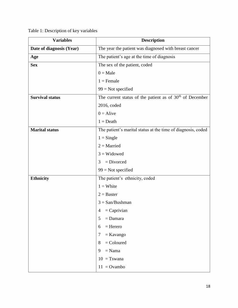
18

Table 1: Description of key variables

Variables Description

Date of diagnosis (Year) The year the patient was diagnosed with breast cancer

Age The patient’s age at the time of diagnosis

Sex The sex of the patient, coded

0 = Male

1 = Female

99 = Not specified

Survival status The current status of the patient as of 30th of December

2016, coded

0 = Alive

1 = Death

Marital status The patient’s marital status at the time of diagnosis, coded

1 = Single

2 = Married

3 = Widowed

3 = Divorced

99 = Not specified

Ethnicity The patient’s ethnicity, coded

1 = White

2 = Baster

3 = San/Bushman

4 = Caprivian

5 = Damara

6 = Herero

7 = Kavango

8 = Coloured

9 = Nama

10 = Tswana

11 = Ovambo

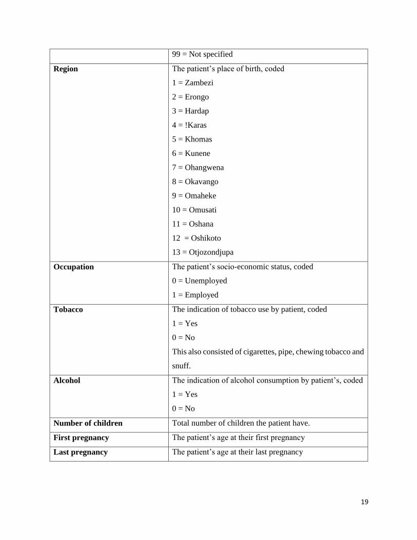
19

99 = Not specified

Region The patient’s place of birth, coded

1 = Zambezi

2 = Erongo

3 = Hardap

4 = !Karas

5 = Khomas

6 = Kunene

7 = Ohangwena

8 = Okavango

9 = Omaheke

10 = Omusati

11 = Oshana

12 = Oshikoto

13 = Otjozondjupa

Occupation The patient’s socio-economic status, coded

0 = Unemployed

1 = Employed

Tobacco The indication of tobacco use by patient, coded

1 = Yes

0 = No

This also consisted of cigarettes, pipe, chewing tobacco and

snuff.

Alcohol The indication of alcohol consumption by patient’s, coded

1 = Yes

0 = No

Number of children Total number of children the patient have.

First pregnancy The patient’s age at their first pregnancy

Last pregnancy The patient’s age at their last pregnancy

20

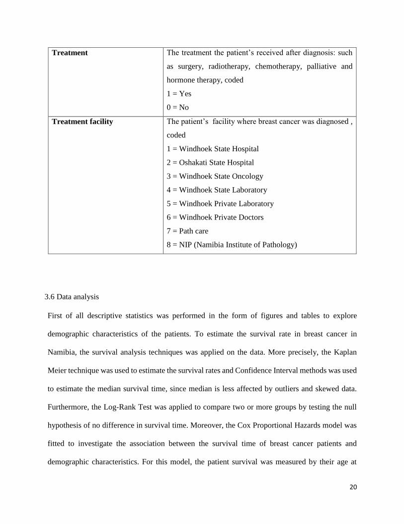
Treatment The treatment the patient’s received after diagnosis: such

as surgery, radiotherapy, chemotherapy, palliative and

hormone therapy, coded

1 = Yes

0 = No

Treatment facility The patient’s facility where breast cancer was diagnosed ,

coded

1 = Windhoek State Hospital

2 = Oshakati State Hospital

3 = Windhoek State Oncology

4 = Windhoek State Laboratory

5 = Windhoek Private Laboratory

6 = Windhoek Private Doctors

7 = Path care

8 = NIP (Namibia Institute of Pathology)

3.6 Data analysis

First of all descriptive statistics was performed in the form of figures and tables to explore

demographic characteristics of the patients. To estimate the survival rate in breast cancer in

Namibia, the survival analysis techniques was applied on the data. More precisely, the Kaplan

Meier technique was used to estimate the survival rates and Confidence Interval methods was used

to estimate the median survival time, since median is less affected by outliers and skewed data.

Furthermore, the Log-Rank Test was applied to compare two or more groups by testing the null

hypothesis of no difference in survival time. Moreover, the Cox Proportional Hazards model was

fitted to investigate the association between the survival time of breast cancer patients and

demographic characteristics. For this model, the patient survival was measured by their age at

21

diagnosis and their age at death. Thus, the event variable for this model was the patient’s status

(alive or dead). On the other hand, the covariates for the Cox Proportional Hazard model were

demographic characteristics of the patients such as their age, marital status, occupation, first

pregnancy, tobacco use, alcohol consumption, ethnicity, sex and region.

3.6.1 Survival analysis

Kleinbaum and Klein (2015) define survival analysis as a collection of statistical procedures for

data analysis for which the outcome variable of interest is time until an event occurs. The time

variable is usually referred to as the survival time, because it gives the time that an individual has

“survived” over some follow-up period. According to Kleinbaum & Klein (2015) there are three

basic goals for survival analysis:

i. To estimate and interpret survivor and/or hazard functions from survival data.

ii. To compare survivor and/or hazard functions and

iii. To assess the relationship of explanatory variables to survival time.

The assumptions for Survival analysis as per Kleinbaum and Klein (2012) are:

i. The data must be heavily skewed and often with censoring

ii. Binary outcomes and survival data outcome which is the time to event must be continuous.

Survival analysis mainly focuses on the survival function, the hazard function and the cumulative

hazard function. A survival function is defined as the probability that an individual will survives

longer than time 𝑡 (Kleinbaum & Klein 2012). Let this function be denoted by 𝑆(𝑡). Thus,

𝑆(𝑡) = 𝑃(𝑇 > 𝑡) (3.1)

22

where 𝑇 is a survival time. 𝑆(𝑡) is a monotonically decreasing function of 𝑡 with the properties:

𝑆(𝑡) = {1 𝑡 = 00 𝑡 = ∞

(3.2)

In other words, the probability of surviving at least time zero is 1, while at an infinite time, the

probability of surviving is 0. The hazard function is defined as the probability of failure during a

very small time interval, assuming that the individual has survived to the beginning of the interval.

It is obtained as

𝑙𝑖𝑚𝑑𝑡→0

Pr(𝑇 ∈ [𝑡, 𝑡 + 𝑑𝑡]|𝑇 ≥ 𝑡)

𝑑𝑡 (3.3)

The cumulative hazard function is defined as the total number of failures or deaths over an interval

of time and it is obtained as

𝐻(𝑡) = ∫ ℎ(𝑢)𝑑𝑢𝑡

0 (3.4)

where ℎ(𝑢) is hazard risk and 𝑢 is accumulated risk

3.6.2 Kaplan Meier

The Kaplan Meier (KM) method is a non-parametric estimates of survival function that is

commonly used to describe the survivorship of a study population and to compare two study

populations (Etikan, Abubakar and Alkassim, 2017). KM estimate is one of the best statistical

methods used to measure the survival probability of patients living for a certain period of time

after treatment. It is a spontaneous graphical (curves) presentation approach and such curves are

used to determine the events, censoring and the survival probability during a given period of time.

According to Etikan et al. (2017), KM estimate is sometimes called the Product Limit (PLI)

23

estimate. This involves computing the probabilities of occurrence of event at a certain point of

time and these successive probabilities are then multiplied by any earlier computed probability to

determine the final estimate. Since in survival analysis, intervals are defined by failures, for

example, the probability of surviving intervals A and B is equal to the probability of surviving

interval A multiplied by the probability of surviving interval B. Therefore the PLI estimate can be

calculated as:

𝑃𝐿𝐼 =𝑃 (𝑆𝑢𝑟𝑣𝑖𝑣𝑖𝑛𝑔 𝑖𝑛𝑡𝑒𝑟𝑣𝑎𝑙 𝐴)

𝑁𝑢𝑚𝑏𝑒𝑟 𝑜𝑓 𝑠𝑢𝑏𝑗𝑒𝑐𝑡 𝑎𝑡 𝑟𝑖𝑠𝑘 𝑢𝑝𝑡𝑜 𝑓𝑎𝑖𝑙𝑢𝑟𝑒 𝐴 ×

𝑃 (𝑆𝑢𝑟𝑣𝑖𝑣𝑖𝑛𝑔 𝑖𝑛𝑡𝑒𝑟𝑣𝑎𝑙 𝐵)

𝑁𝑢𝑚𝑏𝑒𝑟 𝑜𝑓 𝑠𝑢𝑏𝑗𝑒𝑐𝑡 𝑎𝑡 𝑟𝑖𝑠𝑘 𝑢𝑝𝑡𝑜 𝑓𝑎𝑖𝑙𝑢𝑟𝑒 𝐵 (3.5)

The general formula for KM estimation at time 𝑡 when it comes to the survival function is given

by:

Ŝ(𝑡) = ∏ (𝑛𝑗−𝑑𝑗

𝑛𝑗)𝑗|𝑡 𝑗≤𝑡 (3.6)

where 𝑡𝑗 is the time point, 𝑛𝑗 is the number of patient at risk and 𝑑𝑗 is the deaths at time t𝑗 ( Etikan

et al. (2017).

There are three assumptions used in this analysis (Etikan et al. (2017) :

i. At any time participants who are dropped out or censored have the same survival prospects

as those who continue to be followed.

ii. The survival probabilities are the same for participants recruited early and late in the study.

iii. The event occurs at the time specified.

However, the limitation of KM estimate is that it cannot be used for multivariate analysis, because

it only studies the effect of on factor at the time (Etikan et al. 2017).

24

3.6.3 Confidence Interval for Kaplan Meier

From the asymptotic normality of Ŝ(𝑡), a 100(1 − 𝛼)% Confidence Interval (CI) for 𝑆(𝑡) is given

by (Etikan et al. 2017):

Ŝ(𝑡) = ± 𝑍𝛼

2 √𝑉 (Ŝ(𝑡)) (3.7)

where 𝑉 (Ŝ(𝑡)) can be estimated using the Greenwood formula (Kleinbaum and Klein 2012),

which is

𝑉(𝑆(𝑡))̂ = 𝑉 (Ŝ(𝑡))2

∑𝑑(𝑗)

𝑛(𝑗)(𝑛(𝑗) − 𝑑(𝑗))𝑗:𝑦(𝑗)≤𝑡

where 𝑛(𝑗) is the number of patients at risk and 𝑑(𝑗) is the number of death at 𝑡(𝑗)

It is important to note that this CI may contain points outside the [0, 1] interval. Therefore an

appropriate transformation can be used to determine the CI on the transformed scale and then back-

transformed. To illustrate this, consider the log-log transform 𝑙𝑜𝑔(−𝑙𝑜𝑔 𝑆(𝑡)) which takes values

between −∞ and ∞. The CI for this 𝑙𝑜𝑔(−𝑙𝑜𝑔(Ŝ(𝑡))) is given as:

𝑙𝑜𝑔 (−𝑙𝑜𝑔 (Ŝ(𝑡))) ± 𝑍𝛼

2 √𝑉 (log (− log (Ŝ(t)))) (3.8)

where 𝑉 (log (− log (Ŝ(t)))) is approximated using the exponential Greenwood formula

(Kleinbaum and Klein, 2012):

𝑉 (log (− log (Ŝ(t)))) = 1

(𝑙𝑜𝑔Ŝ(𝑡))2∑

𝑑(𝑗)

𝑛(𝑗)(𝑛(𝑗)− 𝑑(𝑗))𝑗:𝑦(𝑗)≤𝑡 (3.9)

Then the CI for 𝑆(𝑡) is obtained through a back-transformation as (Kleinbaum and Klein, 2012):

[Ŝ(𝑡)]𝑒𝑥𝑝 [± 𝑍𝛼

2 √𝑉[𝑙𝑜𝑔(− 𝑙𝑜𝑔(Ŝ(𝑡)))] ]

(3.10)

25

3.6.4 Log-Rank Test

The Log-Rank (LR) test is a large-sample chi-square (𝑥2) test that uses as its test criterion a statistic

that provides an overall comparison of the KM curves being compared (Kleinbaum and Klein,

2015). It is used to test whether the difference between survival times between two groups is

statistically different or not by testing the null hypothesis of significance. The null hypothesis states

that the population do not differ in the probability of an event at any time point. Thus, the LR test

is used in this case to compare these groups if they are the same in the probability of an event at

any time point. The hypotheses and test statistics used in the LR test are described as follow for

two groups of survival (Kleinbaum and Klein, 2015).

Hypotheses:

𝐻0 : 𝑆1(𝑡) = 𝑆2(𝑡) (3.11)

𝐻𝐴 ∶ 𝑆1(𝑡) ≠ 𝑆2(𝑡) (3.12)

Where 𝐻0 = Null hypothesis that the survival curves are identical, 𝐻𝐴 = Alternative hypothesis that

the survival curves are differ, 𝑆1(𝑡) = Survival function of the first group and 𝑆2(𝑡) = Survival

function of the second group.

Test statistic:

𝑥2 = (𝑂1 − 𝐸1)2

𝐸1+

(𝑂2 − 𝐸2)2

𝐸2 (3.13)

where 𝑂1 and 𝑂2 are the observed numbers in groups 1 and 2 respectively, while 𝐸1 and 𝐸2 are

expected numbers of deaths in groups 1 and 2 respectively. This test statistics has approximately

the chi-square distribution with 1 degree of freedom. The expected deaths at time 𝑡 are computed

as:

26

𝑒1𝑡 = 𝑛1𝑡

𝑛1𝑡× 𝑛2𝑡 × 𝑑𝑡 (3.14)

𝑒2𝑡 = 𝑛2𝑡

𝑛1𝑡× 𝑛2𝑡 × 𝑑𝑡 (3.15)

where 𝑑𝑡 is the total deaths for both groups at time 𝑡, 𝑛1𝑡 is total number of patients at risk in

group one and 𝑛2𝑡 is the total number of patients at risk in the second group. Then the total

numbers of deaths expected in the two groups is computed as

𝐸1 = ∑ 𝑒1𝑡∀𝑡 and 𝐸2 = ∑ 𝑒2𝑡∀𝑡 (3.16)

Thus, the Log-Rank test statistic (LR𝑠𝑡𝑎𝑡) is calculated as:

LR𝑠𝑡𝑎𝑡 = (𝑂𝑖 − 𝐸𝑖)2

𝑉𝑎𝑟(𝑂𝑖− 𝐸𝑖) (3.17)

for 𝑖 = 1,2,3 … .. n, with n being the number of patients, and 𝑉𝑎𝑟(𝑂𝑖 − 𝐸𝑖) given by:

𝑉𝑎𝑟(𝑂𝑖 − 𝐸𝑖) = ∑𝑛1𝑡𝑛2𝑡(𝑑1𝑡+𝑑2𝑡)(𝑛1𝑡+𝑛2𝑡−𝑑1𝑡−𝑑2𝑡)

(𝑛1𝑡+𝑛2𝑡)2(𝑛1𝑡+𝑛2𝑡−1)∀𝑡 (3.18)

where 𝑑1𝑡 is the number of death in the first group and 𝑑2𝑡 is the number of death in the second

group.

3.6.5 Cox Proportional Hazard

Since Kaplan Meier and Log-rank test are commonly used for univariate analysis, for the

multivariate analysis, the Cox Proportional Hazard (CPH) models are used.

The CPH model is essentially a regression model used for investigating the association between

the survival time of patients and one or more predictor/explanatory variables (Cox, 1972). This

model works for both quantitative predictor variables and categorical variables. In addition, the

CPH regression model simultaneously assesses the effects of several risk factors on survival time

(LaMorte, 2016). Two key assumptions of the CPH model is that the hazard curves for the groups

27

of observations (or patients) must be proportional and these curves must not interact (LaMorte,

2016). The CPH model is given as:

ℎ𝑖(t) = ℎ0(t)𝑒𝑥𝑝(𝛽𝑋𝑖) (3.19)

where ℎ𝑖(t) is the hazard function for patient 𝑖, ℎ0(t) is the hazard function for a patient in the

control group (i.e., baseline hazard), 𝑒𝑥𝑝(𝛽) is the hazard ratio that measures the effects of the

explanatory/predictor variables on the survival time and 𝑋𝑖 is the explanatory/predictor variables

(Kleinbaum and Klein, 2015). In this study, the explanatory/predictor variables were the patients’

Age, Marital status, Occupation, Tobacco use, Alcohol consumption, Sex, Ethnicity and Place of

residence (Region), Treatment and Treatment facility.

The CPH model has several characteristics as follows (Kleinbaum and Klein, 2015).

(i) It is a semi-parametric model, because all the functions in model are not completely

specified - i.e. the baseline function is not specified.

(ii) It is robust, because it can closely approximate the correct parametric model.

(iii) Even though the baseline hazard is not specified, reasonably good estimates of the

regression coefficients, hazard ratios of interest and adjusted survival curves can be

obtained for a wide variety of data situations.

(iv) The form always ensures that the fitted model will always give non-negative

estimated hazards.

(v) The hazard ratio is calculated without having to estimate the baseline intensity.

(vi) Survivor and hazard curves can be estimated even though the baseline hazard

function is not specified.

28

(vii) It is preferred over the logistic model when survival time information is available

and there is censoring in the data.

For the fitted CPH survival model of this study, the predictor/explanatory variables that were

considered were those who had probability values (p-values) that were less than a 10% significance

level in the performed univariate (KM) analysis. This elimination scheme was used because not

all the predictors in the study data were relevant in the modelling of survival time. If a predictor

has a p-value greater than 10% in the univariate analysis, it is highly unlikely that it will

significantly contribute to a model which includes other predictors.

Microsoft Excel (2013) was used to edit and clean the study data, while the Statistical Package for

Social Scientist (SPSS) version 22 was used to construct and carryout the KM graphs. The R

software version 3.5.1 (Team, 2018) was utilized to perform the fitted CPH modelling.

3.6.6 Research ethics

Ethical approval of this study was obtained from the Research Ethical Committee of the

University of Namibia from The Centre of Postgraduate Studies and Cancer Association of

Namibia. Extracted Data from CAN did not include patient’s identity and are kept in a locked

computer

29

CHAPTER 4: DATA ANALYSIS

4.1 Introduction

The present chapter represented the results obtained from the applied statistical methods or

techniques discussed in chapter 3 in particular, Descriptive statistics, Survival techniques such as:

Kaplan Meier, Log-Rank test and Cox proportional hazard. The results are demonstrated in the

forms of tables, figures and interpreted.

4.2 Descriptive statistics

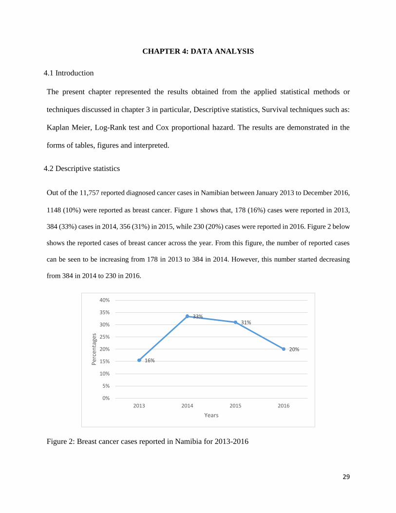
Out of the 11,757 reported diagnosed cancer cases in Namibian between January 2013 to December 2016,

1148 (10%) were reported as breast cancer. Figure 1 shows that, 178 (16%) cases were reported in 2013,

384 (33%) cases in 2014, 356 (31%) in 2015, while 230 (20%) cases were reported in 2016. Figure 2 below

shows the reported cases of breast cancer across the year. From this figure, the number of reported cases

can be seen to be increasing from 178 in 2013 to 384 in 2014. However, this number started decreasing

from 384 in 2014 to 230 in 2016.

Figure 2: Breast cancer cases reported in Namibia for 2013-2016

16%

33%31%

20%

0%

5%

10%

15%

20%

25%

30%

35%

40%

2013 2014 2015 2016

Per

cen

tage

s

Years

30

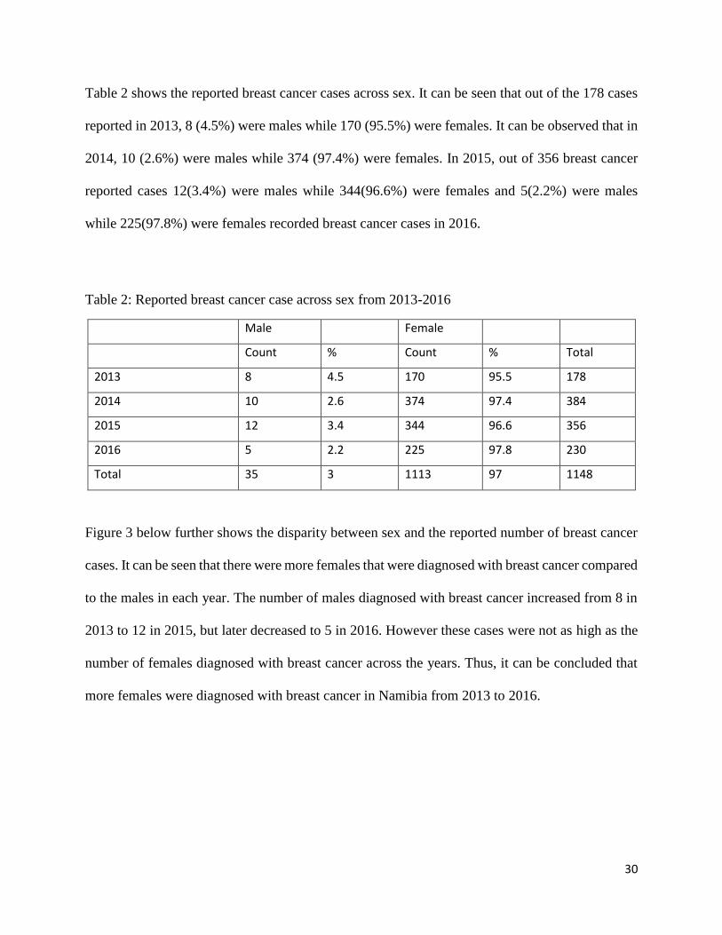
Table 2 shows the reported breast cancer cases across sex. It can be seen that out of the 178 cases

reported in 2013, 8 (4.5%) were males while 170 (95.5%) were females. It can be observed that in

2014, 10 (2.6%) were males while 374 (97.4%) were females. In 2015, out of 356 breast cancer

reported cases 12(3.4%) were males while 344(96.6%) were females and 5(2.2%) were males

while 225(97.8%) were females recorded breast cancer cases in 2016.

Table 2: Reported breast cancer case across sex from 2013-2016

Male Female

Count % Count % Total

2013 8 4.5 170 95.5 178

2014 10 2.6 374 97.4 384

2015 12 3.4 344 96.6 356

2016 5 2.2 225 97.8 230

Total 35 3 1113 97 1148

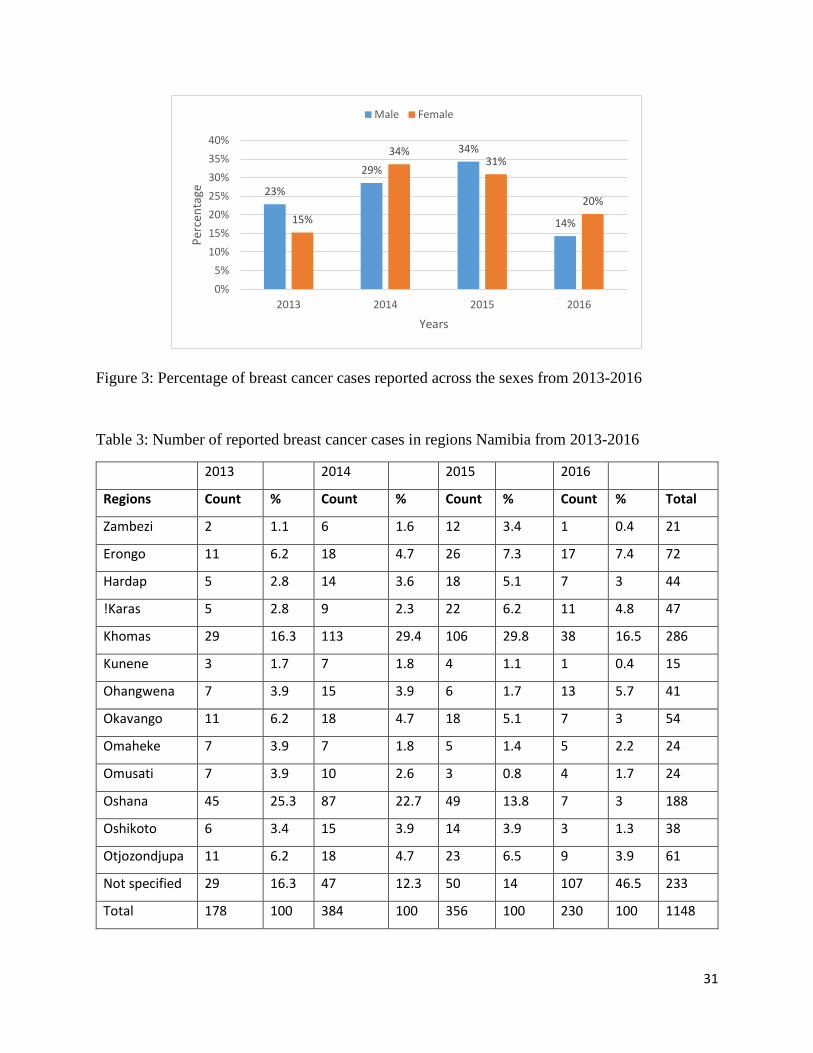
Figure 3 below further shows the disparity between sex and the reported number of breast cancer

cases. It can be seen that there were more females that were diagnosed with breast cancer compared

to the males in each year. The number of males diagnosed with breast cancer increased from 8 in

2013 to 12 in 2015, but later decreased to 5 in 2016. However these cases were not as high as the

number of females diagnosed with breast cancer across the years. Thus, it can be concluded that

more females were diagnosed with breast cancer in Namibia from 2013 to 2016.

31

Figure 3: Percentage of breast cancer cases reported across the sexes from 2013-2016

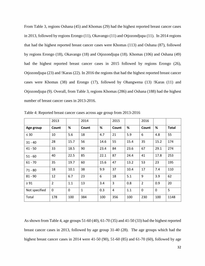
Table 3: Number of reported breast cancer cases in regions Namibia from 2013-2016

2013 2014 2015 2016

Regions Count % Count % Count % Count % Total

Zambezi 2 1.1 6 1.6 12 3.4 1 0.4 21

Erongo 11 6.2 18 4.7 26 7.3 17 7.4 72

Hardap 5 2.8 14 3.6 18 5.1 7 3 44

!Karas 5 2.8 9 2.3 22 6.2 11 4.8 47

Khomas 29 16.3 113 29.4 106 29.8 38 16.5 286

Kunene 3 1.7 7 1.8 4 1.1 1 0.4 15

Ohangwena 7 3.9 15 3.9 6 1.7 13 5.7 41

Okavango 11 6.2 18 4.7 18 5.1 7 3 54

Omaheke 7 3.9 7 1.8 5 1.4 5 2.2 24

Omusati 7 3.9 10 2.6 3 0.8 4 1.7 24

Oshana 45 25.3 87 22.7 49 13.8 7 3 188

Oshikoto 6 3.4 15 3.9 14 3.9 3 1.3 38

Otjozondjupa 11 6.2 18 4.7 23 6.5 9 3.9 61

Not specified 29 16.3 47 12.3 50 14 107 46.5 233

Total 178 100 384 100 356 100 230 100 1148

23%

29%

34%

14%15%

34%31%

20%

0%

5%

10%

15%

20%

25%

30%

35%

40%

2013 2014 2015 2016

Per

cen

tage

Years

Male Female

32

From Table 3, regions Oshana (45) and Khomas (29) had the highest reported breast cancer cases

in 2013, followed by regions Erongo (11), Okavango (11) and Otjozondjupa (11). In 2014 regions

that had the highest reported breast cancer cases were Khomas (113) and Oshana (87), followed

by regions Erongo (18), Okavango (18) and Otjozondjupa (18). Khomas (106) and Oshana (49)

had the highest reported breast cancer cases in 2015 followed by regions Erongo (26),

Otjozondjupa (23) and !Karas (22). In 2016 the regions that had the highest reported breast cancer

cases were Khomas (38) and Erongo (17), followed by Ohangwena (13) !Karas (11) and

Otjozondjupa (9). Overall, from Table 3, regions Khomas (286) and Oshana (188) had the highest

number of breast cancer cases in 2013-2016.

Table 4: Reported breast cancer cases across age group from 2013-2016

2013 2014 2015 2016

Age group Count % Count % Count % Count % Total

≤ 30 10 5.6 18 4.7 21 5.9 6 4.8 55

31 - 40 28 15.7 56 14.6 55 15.4 35 15.2 174

41 - 50 33 18.5 90 23.4 84 23.6 67 29.1 274

51 - 60 40 22.5 85 22.1 87 24.4 41 17.8 253

61 - 70 35 19.7 60 15.6 47 13.2 53 23 195

71 - 80 18 10.1 38 9.9 37 10.4 17 7.4 110

81 - 90 12 6.7 23 6 18 5.1 9 3.9 62

≥ 91 2 1.1 13 3.4 3 0.8 2 0.9 20

Not specified 0 0 1 0.3 4 1.1 0 0 5

Total 178 100 384 100 356 100 230 100 1148

As shown from Table 4, age groups 51-60 (40), 61-70 (35) and 41-50 (33) had the highest reported

breast cancer cases in 2013, followed by age group 31-40 (28). The age groups which had the

highest breast cancer cases in 2014 were 41-50 (90), 51-60 (85) and 61-70 (60), followed by age

33

group 31-40 (56). In 2015 age group 51-60 (87), 41-50 (84) had the highest reported breast cancer

cases, followed by age group 31-40 (55) and 61-70 (47). Consequently in 2016 the age group that

had the highest breast cancer cases were 41-50 (67) and 61-70 (53), followed by 51-60 (41) and

31-40 (35). Last of all, from Table 4, age groups 41-50 (274) and 51-60 (253) had the highest

number of breast cancer cases since 2013-2016.

Table 5: Socio- demographic information of the breast cancer patients

DESCRIPTION COUNT %

SURVIVAL STATUS

Alive 1030 89.6

Death 118 10.3

Total (N) 1148 100

SEX

Male 35 3.0

Female 1113 96.9

Total (N) 1148 100

AGE GROUP

≤ 30 55 4.8

31 - 40 174 15.1

41 - 50 274 23.8

51 – 60 253 22.0

61 – 70 195 17.0

71 – 80 110 9.6

81 – 90 62 5.4

≥ 91 20 1.7

Not specified 5 1.4

Total (N) 1148 100

MARITAL STATUS

34

Single 157 13.7

Married 139 12.1

Widowed 67 5.8

Divorced 18 1.6

Not specified 767 66.8

Total (N) 1148 100

OCCUPATION

Unemployed 84 7.3

Employed 102 8.9


Total (N) 1148 100

TOBACCO USE

No 303 26.4

Yes 71 6.2


Total (N) 1148 100

ALCOHOL

NO 105 9.1

Yes 143 12.4


Total (N) 1148 100

TREATMENT

No 739 64.4

Yes 409 35.6

Total (N) 1148 100

TREATMENT FACILITY

Windhoek State Hospital 271 23.6

Oshakati State Hospital 132 11.5

Windhoek State Oncology 358 31.2

Windhoek State Laboratory 74 6.4

Windhoek Private Laboratory 194 16.9

35

Windhoek Private Doctors 35 3.0

NIP 52 4.5


Total (N) 1148 100

REGION

Not specified 1 .1

Zambezi 21 1.8

Erongo 72 6.3

Hardap 44 3.8

!Karas 47 4.1

Khomas 286 24.9

Kunene 15 1.3

Ohangwena 41 3.6

Okavango 54 4.7

Omaheke 24 2.1

Omusati 24 2.1

Oshana 188 16.4

Oshikoto 38 3.3

Otjozondjupa 61 5.3

Total (N) 1148 100

ETHNICITY

White 76 6.6

Baster 45 3.9

San/Bushman 5 .4

Caprivian 14 1.2

Damara 50 4.4

Herero 43 3.7

Kavango 42 3.7

Coloured 34 3.0

Nama 36 3.1

Tswana 3 .3

36

Ovambo 495 43.1

Total (N) 1148 100

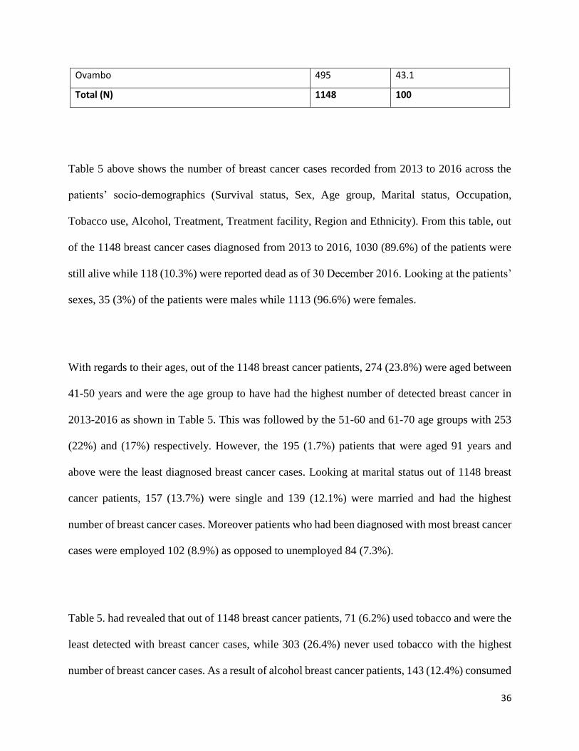
Table 5 above shows the number of breast cancer cases recorded from 2013 to 2016 across the

patients’ socio-demographics (Survival status, Sex, Age group, Marital status, Occupation,

Tobacco use, Alcohol, Treatment, Treatment facility, Region and Ethnicity). From this table, out

of the 1148 breast cancer cases diagnosed from 2013 to 2016, 1030 (89.6%) of the patients were

still alive while 118 (10.3%) were reported dead as of 30 December 2016. Looking at the patients’

sexes, 35 (3%) of the patients were males while 1113 (96.6%) were females.

With regards to their ages, out of the 1148 breast cancer patients, 274 (23.8%) were aged between

41-50 years and were the age group to have had the highest number of detected breast cancer in

2013-2016 as shown in Table 5. This was followed by the 51-60 and 61-70 age groups with 253

(22%) and (17%) respectively. However, the 195 (1.7%) patients that were aged 91 years and

above were the least diagnosed breast cancer cases. Looking at marital status out of 1148 breast

cancer patients, 157 (13.7%) were single and 139 (12.1%) were married and had the highest

number of breast cancer cases. Moreover patients who had been diagnosed with most breast cancer

cases were employed 102 (8.9%) as opposed to unemployed 84 (7.3%).

Table 5. had revealed that out of 1148 breast cancer patients, 71 (6.2%) used tobacco and were the

least detected with breast cancer cases, while 303 (26.4%) never used tobacco with the highest

number of breast cancer cases. As a result of alcohol breast cancer patients, 143 (12.4%) consumed

37

alcohol and had the highest breast cancer cases on contrary with 105 (9.1%) who never consumed

alcohol. As observed in Table 5, out of 1148 breast cancer patients, 409 (35.6%) had received

cancer treatment, but 739 (64.4) did not receive any cancer treatment. With regards to treatment

facility, 358 (31.2%) were diagnosed at Windhoek State Oncology and had the highest number of

breast cancer detection, followed by Windhoek State Hospital 271 (23.6%) and Windhoek Private

Laboratory 194 (16.9%). Least of all was Windhoek Private Doctors 35 (3) recorded with low

breast cancer cases.

Table 5 above indicated that, out of the 1148 breast cancer cases diagnosed from 2013 to 2016,

286 (24.9%) were reported from Khomas region being the highest with breast cancer cases

detected, followed by Oshana region 188 (16.4%). The regions with the least recorded breast

cancer cases were Kunene 15 (1.3%) and Zambezi 21 (1.8%).

Regarding the patients’ ethnicity, Table 5 shows that out of 1148 breast cancer patients, 495

(43.1%) were Ovambo patients and were the ethnic group to have had the highest number of

detected breast cancer in 2013-2016, followed by whites 76 (6.6%) and Damara 50 (4.4%).

However, the Tswana ethnic group 3 (.3%) were the least diagnosed breast cancer cases.

4.3 Survival Analysis

4.3.1 Kaplan Meier (KM)

The KM method described in section 3.5.2 was applied to the 1148 breast cancer cases, where the

response variable (Y) was defined as the survival time and predictors (𝑋s) were Sex, Age group,

Occupation, Tobacco use, Alcohol, Marital status, Ethnicity, Region, Treatment, Treatment

38

facility and Date of diagnosis. That is, 𝑋1 = 𝑆𝑒𝑥, 𝑋2 = 𝐴𝑔𝑒, 𝑋3 = 𝑂𝑐𝑐𝑢𝑝𝑎𝑡𝑖𝑜𝑛, 𝑋4 = 𝑇𝑜𝑏𝑎𝑐𝑐𝑜

use, 𝑋5 = 𝐴𝑙𝑐𝑜ℎ𝑜𝑙, 𝑋6 = 𝑀𝑎𝑟𝑖𝑡𝑎𝑙 𝑠𝑡𝑎𝑡𝑢𝑠, 𝑋7 = 𝐸𝑡ℎ𝑛𝑖𝑐ity, 𝑋8 = 𝑅𝑒𝑔𝑖𝑜𝑛, 𝑋9 = 𝑇𝑟𝑒𝑎𝑡𝑚𝑒𝑛𝑡,

𝑋10 = 𝑇𝑟𝑒𝑎𝑡𝑚𝑒𝑛𝑡 𝑓𝑎𝑐𝑖𝑙𝑖𝑡𝑦, and 𝑋12 = 𝐷𝑎𝑡𝑒 𝑜𝑓 𝑑𝑖𝑎𝑔𝑛𝑜𝑠𝑖𝑠.

The survival time of a patient was calculated as

Ŝ(𝑡) = ∏ (𝑛𝑗 − 𝑑𝑗

𝑛𝑗)

𝑗|𝑡 𝑗≤𝑡

(4.1)

where 𝑡𝑗 is the time point, 𝑛𝑗 is the number of patient at risk and 𝑑𝑗 is the deaths at time t𝑗 (Etikan

et al., (2017).

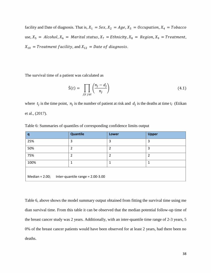
Table 6: Summaries of quantiles of corresponding confidence limits output

q Quantile Lower Upper

25% 3 3 3

50% 2 2 3

75% 2 2 2

100% 1 1 1

Median = 2.00; Inter-quantile range = 2.00-3.00

Table 6, above shows the model summary output obtained from fitting the survival time using me

dian survival time. From this table it can be observed that the median potential follow-up time of

the breast cancer study was 2 years. Additionally, with an inter-quantile time range of 2-3 years, 5

0% of the breast cancer patients would have been observed for at least 2 years, had there been no

deaths.

39

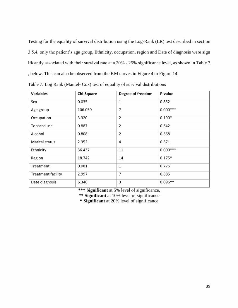
Testing for the equality of survival distribution using the Log-Rank (LR) test described in section

3.5.4, only the patient’s age group, Ethnicity, occupation, region and Date of diagnosis were sign

ificantly associated with their survival rate at a 20% - 25% significance level, as shown in Table 7

, below. This can also be observed from the KM curves in Figure 4 to Figure 14.

Table 7: Log Rank (Mantel- Cox) test of equality of survival distributions

Variables Chi-Square Degree of freedom P-value

Sex 0.035 1 0.852

Age group 106.059 7 0.000***

Occupation 3.320 2 0.190*

Tobacco use 0.887 2 0.642

Alcohol 0.808 2 0.668

Marital status 2.352 4 0.671

Ethnicity 36.437 11 0.000***

Region 18.742 14 0.175*

Treatment 0.081 1 0.776

Treatment facility 2.997 7 0.885

Date diagnosis 6.346 3 0.096**

*** Significant at 5% level of significance,

** Significant at 10% level of significance

* Significant at 20% level of significance

40

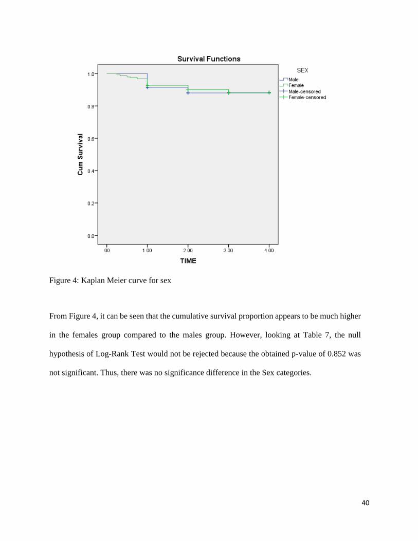
Figure 4: Kaplan Meier curve for sex

From Figure 4, it can be seen that the cumulative survival proportion appears to be much higher

in the females group compared to the males group. However, looking at Table 7, the null

hypothesis of Log-Rank Test would not be rejected because the obtained p-value of 0.852 was

not significant. Thus, there was no significance difference in the Sex categories.

41

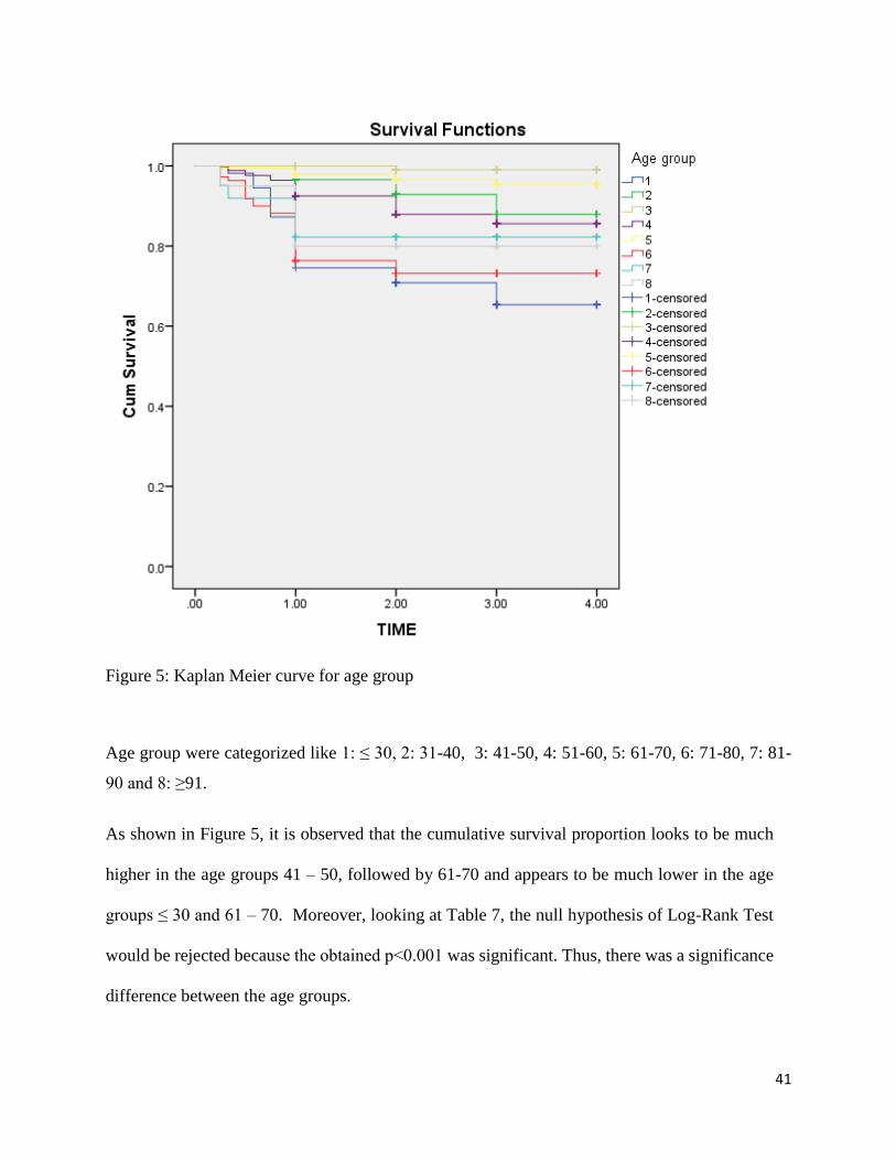
Figure 5: Kaplan Meier curve for age group

Age group were categorized like 1: ≤ 30, 2: 31-40, 3: 41-50, 4: 51-60, 5: 61-70, 6: 71-80, 7: 81-

90 and 8: ≥91.

As shown in Figure 5, it is observed that the cumulative survival proportion looks to be much

higher in the age groups 41 – 50, followed by 61-70 and appears to be much lower in the age

groups ≤ 30 and 61 – 70. Moreover, looking at Table 7, the null hypothesis of Log-Rank Test

would be rejected because the obtained p˂0.001 was significant. Thus, there was a significance

difference between the age groups.

42

Figure 6: Kaplan Meier curve for Occupation

Figure 6, shows that the cumulative survival proportion appears to be much higher in the patients

who were employed compared to the unemployed patients. Besides, looking at Table 7, the null

hypothesis of Log-Rank Test would not be rejected because the obtained p-value of 0.190 was

not significant. Thus, there was no significance difference between the occupation categories.

43

Figure 7: Kaplan Meier curve for Tobacco use

As shown in Figure 7, the cumulative survival proportion appears to be much higher in the

patients who did not use tobacco compared to the patients who used tobacco. Observing from

Table 7, the null hypothesis of Log-Rank Test would not be rejected because the obtained p-

value of 0.642 was not significant. Thus, there was no significance difference between the

tobacco use categories.

44

Figure 8: Kaplan Meier curve for Alcohol

Figure 8, shows that the cumulative survival proportion appears to be much higher in the patients

who never consumed alcohol compared to the patients who consumed alcohol. However, as

observed from Table 7, the null hypothesis of Log-Rank Test would not be rejected because the

obtained p-value of 0.668 was not significant. Thus, there was no significance difference

between the patients that consumed alcohol and never consumed.

45

Figure 9: Kaplan Meier curve for Marital status


higher among patients who were married, followed by single patients. It appears to be much

lower in widowed patients. After all, by looking at Table 7, the null hypothesis of Log-Rank

Test would not be rejected because the obtained p-value of 0.671 was not significant. Hence,

there was no significance difference between the marital statuses.

46

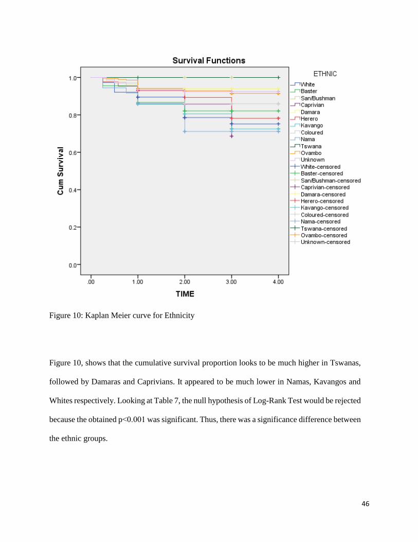
Figure 10: Kaplan Meier curve for Ethnicity

Figure 10, shows that the cumulative survival proportion looks to be much higher in Tswanas,

followed by Damaras and Caprivians. It appeared to be much lower in Namas, Kavangos and

Whites respectively. Looking at Table 7, the null hypothesis of Log-Rank Test would be rejected

because the obtained p˂0.001 was significant. Thus, there was a significance difference between

the ethnic groups.

47

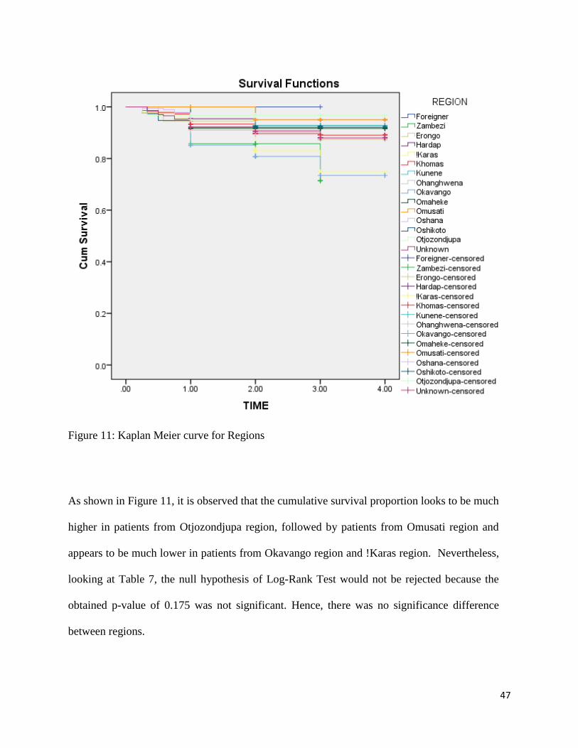
Figure 11: Kaplan Meier curve for Regions


higher in patients from Otjozondjupa region, followed by patients from Omusati region and

appears to be much lower in patients from Okavango region and !Karas region. Nevertheless,

looking at Table 7, the null hypothesis of Log-Rank Test would not be rejected because the

obtained p-value of 0.175 was not significant. Hence, there was no significance difference

between regions.

48

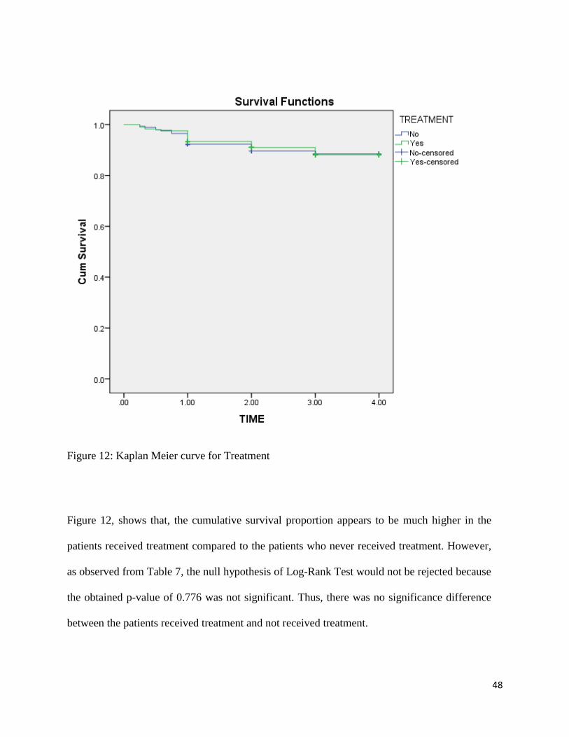
Figure 12: Kaplan Meier curve for Treatment

Figure 12, shows that, the cumulative survival proportion appears to be much higher in the

patients received treatment compared to the patients who never received treatment. However,

as observed from Table 7, the null hypothesis of Log-Rank Test would not be rejected because

the obtained p-value of 0.776 was not significant. Thus, there was no significance difference

between the patients received treatment and not received treatment.

49

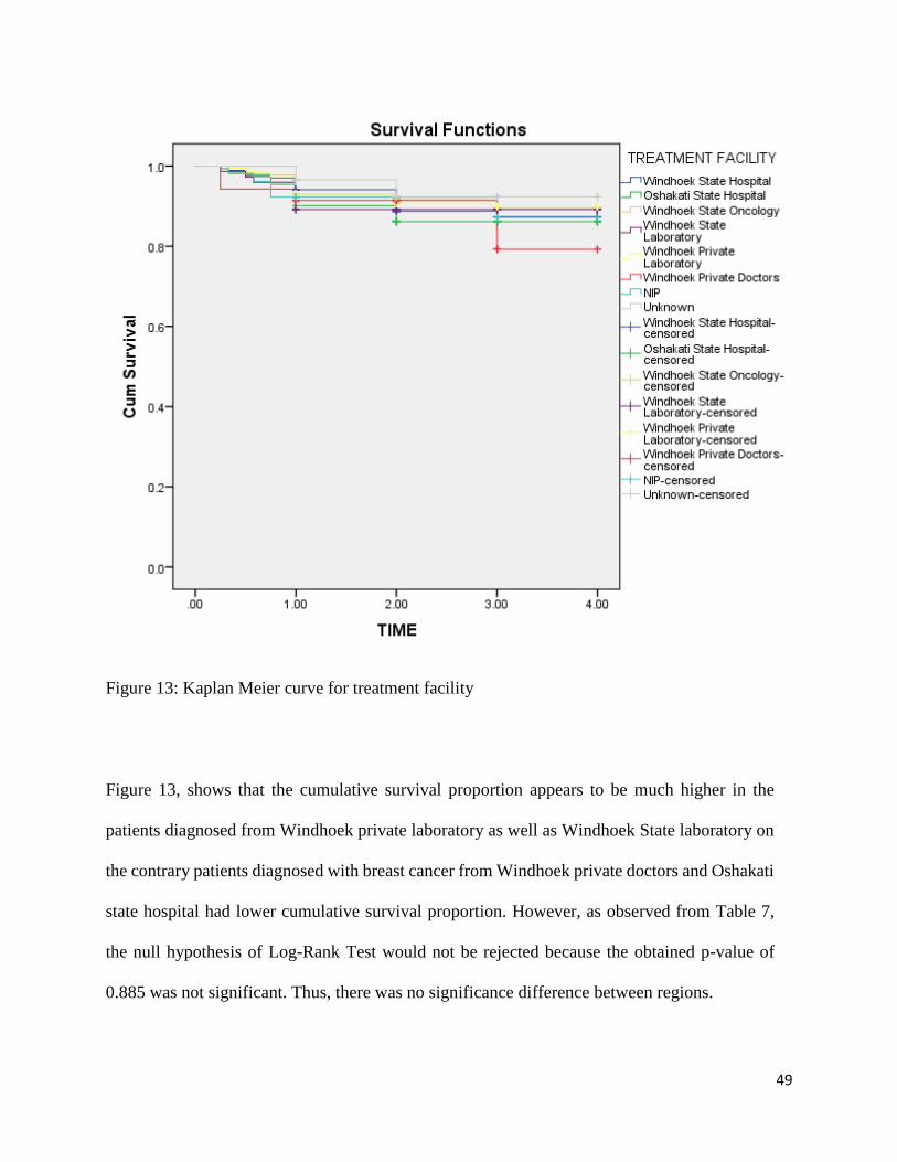
Figure 13: Kaplan Meier curve for treatment facility

Figure 13, shows that the cumulative survival proportion appears to be much higher in the

patients diagnosed from Windhoek private laboratory as well as Windhoek State laboratory on

the contrary patients diagnosed with breast cancer from Windhoek private doctors and Oshakati

state hospital had lower cumulative survival proportion. However, as observed from Table 7,

the null hypothesis of Log-Rank Test would not be rejected because the obtained p-value of

0.885 was not significant. Thus, there was no significance difference between regions.

50

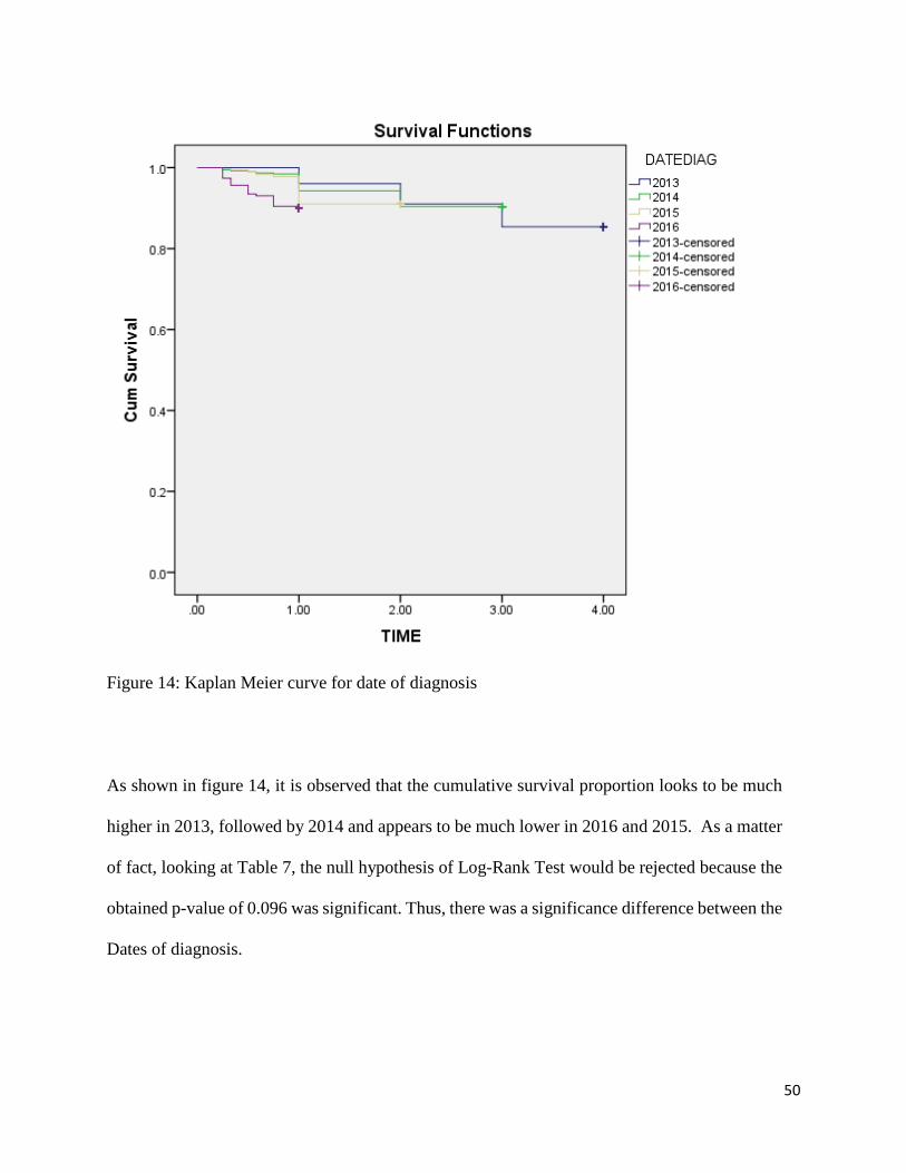
Figure 14: Kaplan Meier curve for date of diagnosis

As shown in figure 14, it is observed that the cumulative survival proportion looks to be much

higher in 2013, followed by 2014 and appears to be much lower in 2016 and 2015. As a matter

of fact, looking at Table 7, the null hypothesis of Log-Rank Test would be rejected because the

obtained p-value of 0.096 was significant. Thus, there was a significance difference between the

Dates of diagnosis.

51

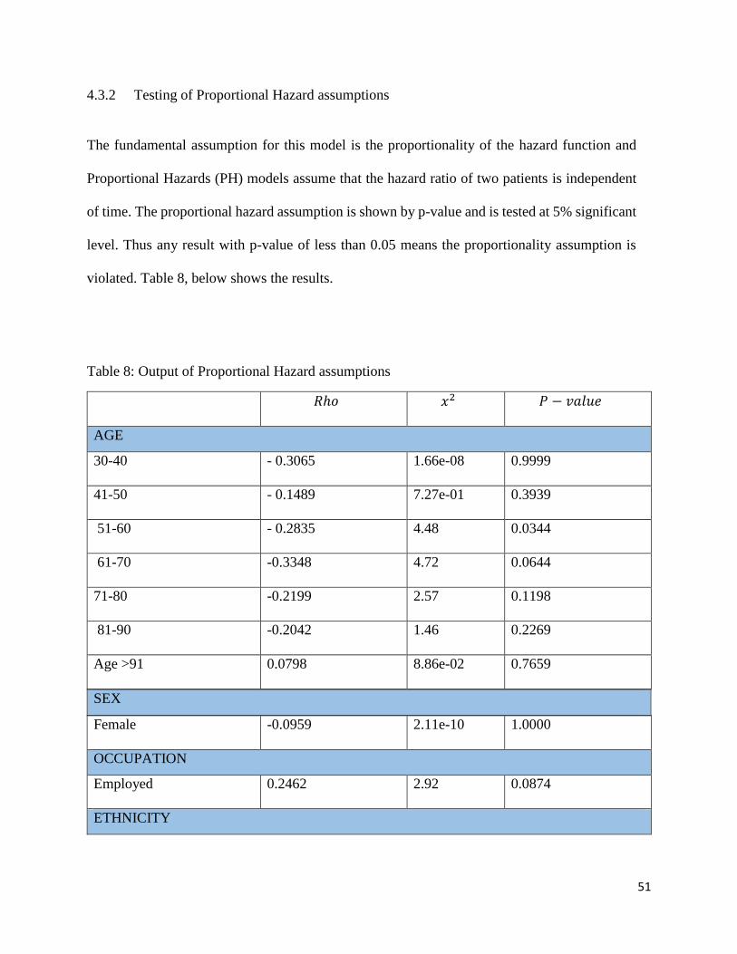
4.3.2 Testing of Proportional Hazard assumptions

The fundamental assumption for this model is the proportionality of the hazard function and

Proportional Hazards (PH) models assume that the hazard ratio of two patients is independent

of time. The proportional hazard assumption is shown by p-value and is tested at 5% significant

level. Thus any result with p-value of less than 0.05 means the proportionality assumption is

violated. Table 8, below shows the results.

Table 8: Output of Proportional Hazard assumptions

𝑅ℎ𝑜 𝑥2 𝑃 − 𝑣𝑎𝑙𝑢𝑒

AGE

30-40 - 0.3065 1.66e-08 0.9999

41-50 - 0.1489 7.27e-01 0.3939

51-60 - 0.2835 4.48 0.0344

61-70 -0.3348 4.72 0.0644

71-80 -0.2199 2.57 0.1198

81-90 -0.2042 1.46 0.2269

Age >91 0.0798 8.86e-02 0.7659

SEX

Female -0.0959 2.11e-10 1.0000

OCCUPATION

Employed 0.2462 2.92 0.0874

ETHNICITY

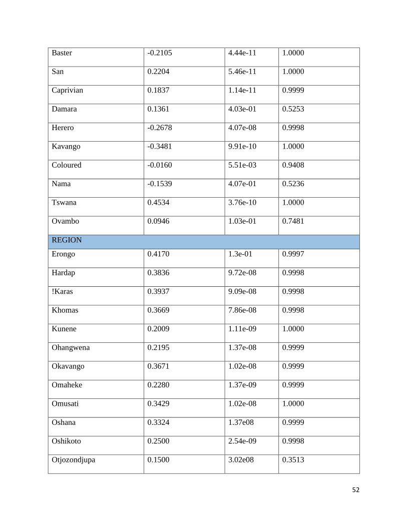
52

Baster -0.2105 4.44e-11 1.0000

San 0.2204 5.46e-11 1.0000

Caprivian 0.1837 1.14e-11 0.9999

Damara 0.1361 4.03e-01 0.5253

Herero -0.2678 4.07e-08 0.9998

Kavango -0.3481 9.91e-10 1.0000

Coloured -0.0160 5.51e-03 0.9408

Nama -0.1539 4.07e-01 0.5236

Tswana 0.4534 3.76e-10 1.0000

Ovambo 0.0946 1.03e-01 0.7481

REGION

Erongo 0.4170 1.3e-01 0.9997

Hardap 0.3836 9.72e-08 0.9998

!Karas 0.3937 9.09e-08 0.9998

Khomas 0.3669 7.86e-08 0.9998

Kunene 0.2009 1.11e-09 1.0000

Ohangwena 0.2195 1.37e-08 0.9999

Okavango 0.3671 1.02e-08 0.9999

Omaheke 0.2280 1.37e-09 0.9999

Omusati 0.3429 1.02e-08 1.0000

Oshana 0.3324 1.37e08 0.9999

Oshikoto 0.2500 2.54e-09 0.9998

Otjozondjupa 0.1500 3.02e08 0.3513

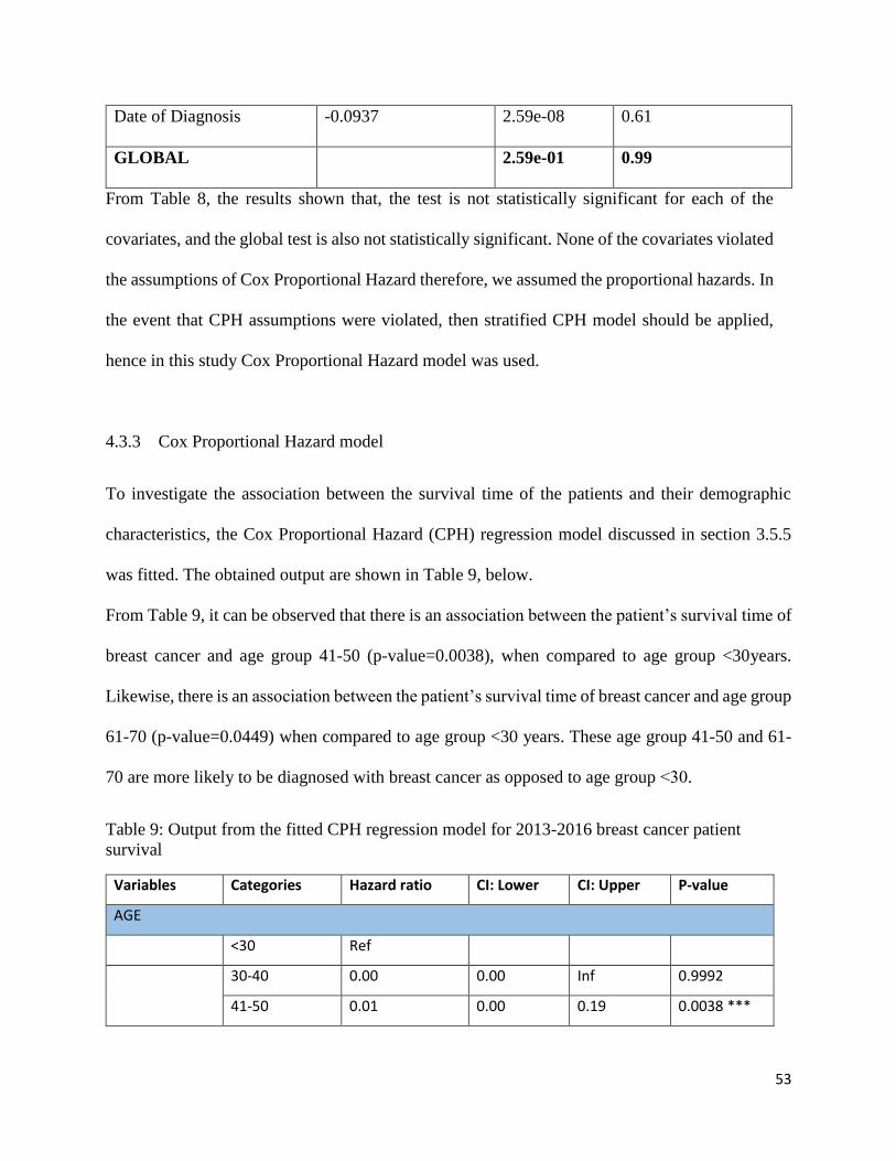
53

Date of Diagnosis -0.0937 2.59e-08 0.61

GLOBAL 2.59e-01 0.99

From Table 8, the results shown that, the test is not statistically significant for each of the

covariates, and the global test is also not statistically significant. None of the covariates violated

the assumptions of Cox Proportional Hazard therefore, we assumed the proportional hazards. In

the event that CPH assumptions were violated, then stratified CPH model should be applied,

hence in this study Cox Proportional Hazard model was used.

4.3.3 Cox Proportional Hazard model

To investigate the association between the survival time of the patients and their demographic

characteristics, the Cox Proportional Hazard (CPH) regression model discussed in section 3.5.5

was fitted. The obtained output are shown in Table 9, below.

From Table 9, it can be observed that there is an association between the patient’s survival time of

breast cancer and age group 41-50 (p-value=0.0038), when compared to age group <30years.

Likewise, there is an association between the patient’s survival time of breast cancer and age group

61-70 (p-value=0.0449) when compared to age group <30 years. These age group 41-50 and 61-

70 are more likely to be diagnosed with breast cancer as opposed to age group ˂30.

Table 9: Output from the fitted CPH regression model for 2013-2016 breast cancer patient

survival

Variables Categories Hazard ratio CI: Lower CI: Upper P-value

AGE

<30 Ref

30-40 0.00 0.00 Inf 0.9992

41-50 0.01 0.00 0.19 0.0038 ***

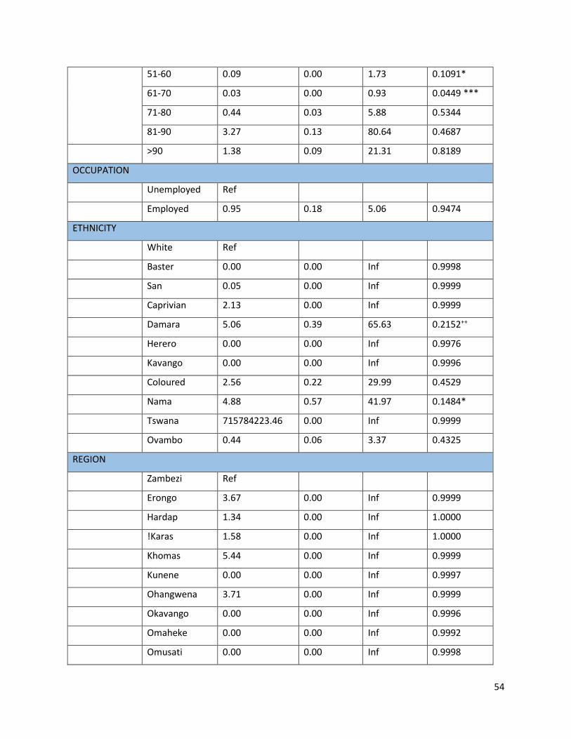
54

51-60 0.09 0.00 1.73 0.1091*

61-70 0.03 0.00 0.93 0.0449 ***

71-80 0.44 0.03 5.88 0.5344

81-90 3.27 0.13 80.64 0.4687

>90 1.38 0.09 21.31 0.8189

OCCUPATION

Unemployed Ref

Employed 0.95 0.18 5.06 0.9474

ETHNICITY

White Ref

Baster 0.00 0.00 Inf 0.9998

San 0.05 0.00 Inf 0.9999

Caprivian 2.13 0.00 Inf 0.9999

Damara 5.06 0.39 65.63 0.2152++

Herero 0.00 0.00 Inf 0.9976

Kavango 0.00 0.00 Inf 0.9996

Coloured 2.56 0.22 29.99 0.4529

Nama 4.88 0.57 41.97 0.1484*

Tswana 715784223.46 0.00 Inf 0.9999

Ovambo 0.44 0.06 3.37 0.4325

REGION

Zambezi Ref

Erongo 3.67 0.00 Inf 0.9999

Hardap 1.34 0.00 Inf 1.0000

!Karas 1.58 0.00 Inf 1.0000

Khomas 5.44 0.00 Inf 0.9999

Kunene 0.00 0.00 Inf 0.9997

Ohangwena 3.71 0.00 Inf 0.9999

Okavango 0.00 0.00 Inf 0.9996

Omaheke 0.00 0.00 Inf 0.9992

Omusati 0.00 0.00 Inf 0.9998

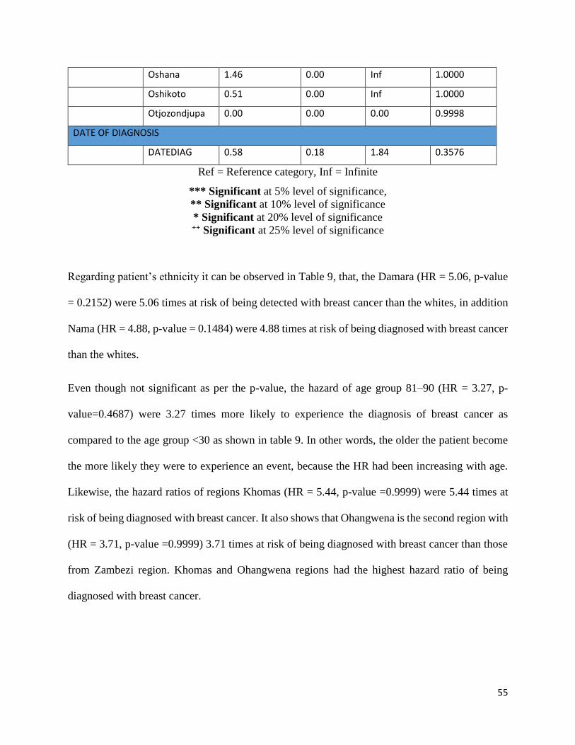
55

Oshana 1.46 0.00 Inf 1.0000

Oshikoto 0.51 0.00 Inf 1.0000

Otjozondjupa 0.00 0.00 0.00 0.9998

DATE OF DIAGNOSIS

DATEDIAG 0.58 0.18 1.84 0.3576

Ref = Reference category, Inf = Infinite

*** Significant at 5% level of significance,

** Significant at 10% level of significance

* Significant at 20% level of significance ++ Significant at 25% level of significance

Regarding patient’s ethnicity it can be observed in Table 9, that, the Damara (HR = 5.06, p-value

= 0.2152) were 5.06 times at risk of being detected with breast cancer than the whites, in addition

Nama (HR = 4.88, p-value = 0.1484) were 4.88 times at risk of being diagnosed with breast cancer

than the whites.

Even though not significant as per the p-value, the hazard of age group 81–90 (HR = 3.27, p-

value=0.4687) were 3.27 times more likely to experience the diagnosis of breast cancer as

compared to the age group <30 as shown in table 9. In other words, the older the patient become

the more likely they were to experience an event, because the HR had been increasing with age.

Likewise, the hazard ratios of regions Khomas (HR = 5.44, p-value =0.9999) were 5.44 times at

risk of being diagnosed with breast cancer. It also shows that Ohangwena is the second region with

(HR = 3.71, p-value =0.9999) 3.71 times at risk of being diagnosed with breast cancer than those

from Zambezi region. Khomas and Ohangwena regions had the highest hazard ratio of being

diagnosed with breast cancer.

56

CHAPTER 5: GENERAL DISCUSSION, CONCLUSION AND RECOMMENDATIONS

5.1 INTRODUCTION

This chapter had general discussion in relation to the research objectives. The discussion was

extracted from the results of the study as they relate to the reviewed literature on breast cancer and

other relevant empirical studies.

5.2 GENERAL DISCUSSION

The study revealed that breast cancer can affect anybody regardless of sex in Namibia. Since 2013

to 2016, 3% were males diagnosed with breast cancer, while 97% were females diagnosed with

breast cancer in this study. From 2013 to 2016, 64% of breast cancer patients had not received any

treatment and 36% patients had received. The regions with the most detected breast cancer were

Khomas and Oshana. Results showed that the survival rate of breast cancer was influenced by age

group, and ethnicity. These findings were in agreement with the study done by Pazvakawambwa

& Embula (2017), however their study indicated that region also influenced the cancer survival

rate, but in this study region was not significant, although date of diagnosis showed statistical

significance in this study. Vambo people were the most diagnosed with breast cancer followed by

Whites. Factors that were significantly associated with breast cancer were age category of 41-50

and 61-70 years and ethnicity. In addition the Hazard ratio of breast cancer was 3.27 times in the

age category of 81-90 to develop breast cancer, which is higher than age group ˂30, even though

was not statistically significant. The older the patient become the more likely they were to

experience an event, because the HR had been increasing with age and this is in agreement with

what was mentioned in section 1.2 in the study by Carrara (2017) “indicated that annual incidence

57

has increased with older age group, escalating at 189.1 per 100 000 in women in the 70-74 years

of age”.

As a matter of fact Breyer et al. (2018) found out that older age groups were associated with the

development of breast cancer, which corresponded with the results in this study. Despite this fact,

study done in São Paulo, Brazil by Ferraz and Moreira (2016), indicated that age was not significant

to the presence of competing risk, neither in Cox models (Ferraz and Moreira 2016). The median

survival point was 2 years and this means that 98% of breast cancer patients were still alive at the

end of the study in 2016.

5.3 CONCLUSION

The research concluded that age, ethnicity and date of diagnosis were associated with breast cancer

in Namibia. Breast cancer awareness programmes should emphasis on early screening and impart

more knowledge to women and men in Khomas region as well as in Oshana region. Further

research should be done on age categories 41-50 and 61-70 and see other competing risks (such as

HIV and cancer related diseases) of breast cancer associated with these age groups. In order to

have timely and accuracy breast cancer prevalence and trends in the country, Cancer Association

of Namibia (CAN) need to update their cancer registry, capture data on time, because even 2017

data supposed to be included in this study, but they were not yet entered into the cancer registry.

Subsequently CAN should follow up on breast cancer patients to find out if they are still alive or

not and properly indicate the date of death in their database.

58

5.4 RECOMMENDATIONS

The research study recommends that a greater focus along the breast cancer care pathway in

Namibia, with emphases on improving access to early diagnosis at early age.

The study suggests that the Ministry of Health and Social Services should draft up the country’s

first national policy on breast cancer diagnosis and management, because at the moment there is

none.

The breast cancer screening and awareness campaigns should concentrate on the Vambos, Whites

and Damara communities since they had the highest percentage of reported breast cancer cases

from 2013 to 2016 and this invites for further research on what are the contributing factors for

breast cancer prevalence among these communities.

Further studies on this topic can be done focusing on Khomas region and Oshana Region since

they had the highest reported breast cancer cases from 2013 to 2016. Other researchers should

consider exploring different statistical models apart from CPH. There is a need of adding other

predictors such as family health history of breast cancer and use of contraceptives to the data for

more in-depth analysis.

59

REFERENCES

Abadi, A., Yavari, P., Dehghani-Arani, M., Alavi-Majd, H., Ghasemi, E., Amanpour, F., & Bajdik,

C. (2014). Cox Models Survival Analysis Based on Breast Cancer Treatment. 124-129.

Retrieved May 31, 2018, from https://www.ncbi.nlm.nih.gov/pmc/articles/PMC4171826

Breyer, J. Z., Wendland, E. M., Kops, N. L., Caleffi, M., & Hammes, L. S. (2018). Assessment of

potential risk factors for breast cancer in a population in Southern Brazil. Springer Nature,

169(1), 121-131. Retrieved June 21, 2018, from

https://link.springer.com/article/10.1007/s10549-017-4655-0

Bruin, J. (2016, 02). UCLA Institute for Digital Research and Education: idre. Retrieved May 31,

2018, from https://stats.idre.ucla.edu/stata/seminars/stata-survival/.

Carrara, H. (2017). Cancer incidences in Namibia 2010 - 2014: Namibia National Cancer Registry

(NNCR). Windhoek: Namibia National Cancer Registry (NNCR). Retrieved July 15, 2018

Etikan, İ., Abubakar, S., & Alkassim, R. (2017). The Kaplan Meier Estimate in Survival Analysis.

MedCrave - Biometrics & Biostatistics International Journal, 1-5. Retrieved July 15, 2018

Ferraz, O. R., & Moreira-Filho, C. D. (2016). Survival analysis of women with breast cancer:

competing risk models. Brazil: University of Campinas. doi:10.1590/1413-

812320172211.05092016

Fine, J. P., & Gray, R. J. (1999). A Proportional Hazards Model for the subdistribution of a

competing risk. Journal of the American statistical association, 94(446), 496-509.

Goel, K. M., Khanna, P., & Kishore, J. (2010). Understanding Survival analysis: Kaplan-Meier

estimate. International Journal of Ayurveda Research, 274-278. Retrieved August 07,

2018

Hejmadi, M. (2010). Introduction to Cancer Biology. In H. Momna, How cancer arises. London:

Ventus. Retrieved August 07, 2018

Iita, S. (2009). Woman's awareness knowledge regarding health promotion on prevention of breast

and cervical cancer in Oshakati health district. University of Namibia. Retrieved from

https://repository.unam.edu.na/handle/11070/498.

60

Johnson, L. L., & Shih, H. J. (2012). Principles and Practice of Clinical Research 3rd Edition.

Science Direct, 285-293. Retrieved September 26, 2018

Keele, L. (2010). Proportionally Difficult: Testing for Nonproportional Hazards in Cox Models.

Columus: Ohio State University. Retrieved September 26, 2018

Kleinbaum , D. G., & Klein, M. (2012). Survival analysis (Vol.3). Springer.

Kleinbaum, G. D., & Klein, M. (2015). Survival Analysis - A Self Learning Text. Springer.

LaMorte, W. W. (2016). Cox Proportional Hazards Regression Analysis. Boston: Boston

University School of Public Health. Retrieved September 27, 2018

Lince-Deroche, N., Rensburg, v. C., Masuku, S., Rayne, S., Benn, C., & Holele, P. (2017). Breast

Cancer in South Africa. Johannesburg: University of Witwatersrand - Department of

Internal Medicine. Retrieved September 27, 2018

Mowa, K. A. (2016). An exploration of knowledge, attitudes and practices and other breast cancer

determinants influencing early detection among women in Windhoek. University of

Namibia. Retrieved September 28, 2018, from

http://repository.unam.edu.na/bitstream/handle/11070/1853

Namibia statistics Agency, National Planning Commission. (2011). Namibia 2011 Population and

Housing Census Preliminary Results. Windhoek: NSA.

Pazvakawambwa, L., & Embula, S. P. (2017). Prevalence, trends and risk factors of Breast Cancer

Mortality in Namibia: 2000-2015. Windhoek: The University of Namibia. Retrieved

September 28, 2018

Rich, T. J., Neely, G. J., Paniello, C. R., Voelker, C. C., Nussenbaum, B., & Wang, W. E. (2014).

A practical guide to understanding Kaplan-Meier Curves. PMC, 331-336.

Team, R. C. (2018). R: A language and environment for statistical computing.

Tin, T. S., Elwood, M. J., Brown, C., Sarfati, D., Campbell, I., Scott, N., . . . Lawrenson, R. (2018).

Ethnic disparities in breast cancer survival in New Zealand: which factors contribute?

BioMed Central. Retrieved September 28, 2018

61

Tolley, H. D., Barnes, J. M., & Freeman, M. D. (2016). Survival Analysis in Forensic

Epidemiology. ScienceDirect, 261 - 284.

Vanderpuye, V., Grover, S., Hammad, N., Poojaprabhakar, Simonds, H., Olopade, F., & Stefan,

D. C. (2017). An update on the management of breast cancer in Africa. BioMed Central,

8-12.

Vorobiof, D., Sitas, F., & Vorobiof , G. (2014). Breast Cancer incidence in South Africa. Clinical

Oncology - CANSA, 125-127. Retrieved September 29, 2018

WHO. (2014). World cancer factsheet: World cancer burden (2012). (International Agency for

Research on Cancer Report). United Kingdom (UK): World Health Organisation.

Young, A., Van Niekerk, C. F., & Mogotlane, S. (n.d.). Juta's Manual of Nursing.

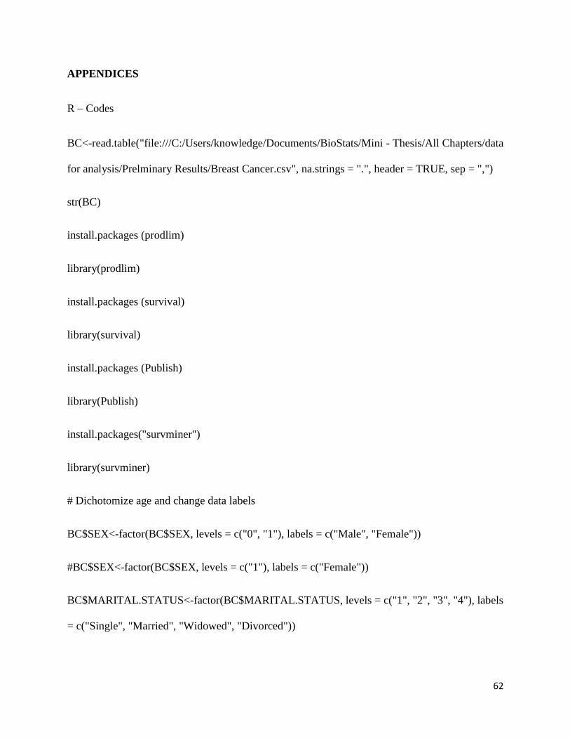
62

APPENDICES

R – Codes

BC<-read.table("file:///C:/Users/knowledge/Documents/BioStats/Mini - Thesis/All Chapters/data

for analysis/Prelminary Results/Breast Cancer.csv", na.strings = ".", header = TRUE, sep = ",")

str(BC)

install.packages (prodlim)

library(prodlim)

install.packages (survival)

library(survival)

install.packages (Publish)

library(Publish)

install.packages("survminer")

library(survminer)

# Dichotomize age and change data labels

BC$SEX<-factor(BC$SEX, levels = c("0", "1"), labels = c("Male", "Female"))

#BC$SEX<-factor(BC$SEX, levels = c("1"), labels = c("Female"))

BC$MARITAL.STATUS<-factor(BC$MARITAL.STATUS, levels = c("1", "2", "3", "4"), labels

= c("Single", "Married", "Widowed", "Divorced"))

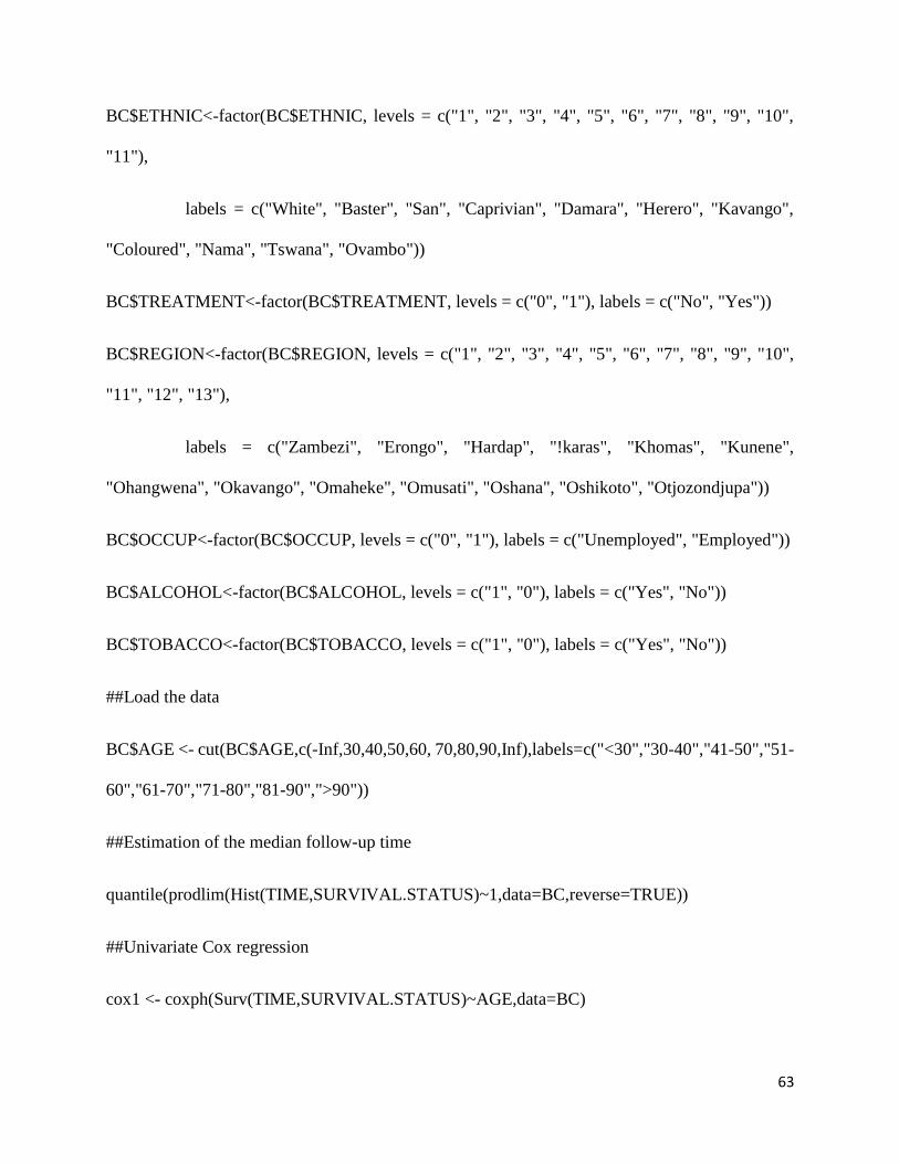
63

BC$ETHNIC<-factor(BC$ETHNIC, levels = c("1", "2", "3", "4", "5", "6", "7", "8", "9", "10",

"11"),

labels = c("White", "Baster", "San", "Caprivian", "Damara", "Herero", "Kavango",

"Coloured", "Nama", "Tswana", "Ovambo"))

BC$TREATMENT<-factor(BC$TREATMENT, levels = c("0", "1"), labels = c("No", "Yes"))

BC$REGION<-factor(BC$REGION, levels = c("1", "2", "3", "4", "5", "6", "7", "8", "9", "10",

"11", "12", "13"),

labels = c("Zambezi", "Erongo", "Hardap", "!karas", "Khomas", "Kunene",

"Ohangwena", "Okavango", "Omaheke", "Omusati", "Oshana", "Oshikoto", "Otjozondjupa"))

BC$OCCUP<-factor(BC$OCCUP, levels = c("0", "1"), labels = c("Unemployed", "Employed"))

BC$ALCOHOL<-factor(BC$ALCOHOL, levels = c("1", "0"), labels = c("Yes", "No"))

BC$TOBACCO<-factor(BC$TOBACCO, levels = c("1", "0"), labels = c("Yes", "No"))

##Load the data

BC$AGE <- cut(BC$AGE,c(-Inf,30,40,50,60, 70,80,90,Inf),labels=c("<30","30-40","41-50","51-

60","61-70","71-80","81-90",">90"))

##Estimation of the median follow-up time

quantile(prodlim(Hist(TIME,SURVIVAL.STATUS)~1,data=BC,reverse=TRUE))

##Univariate Cox regression

cox1 <- coxph(Surv(TIME,SURVIVAL.STATUS)~AGE,data=BC)

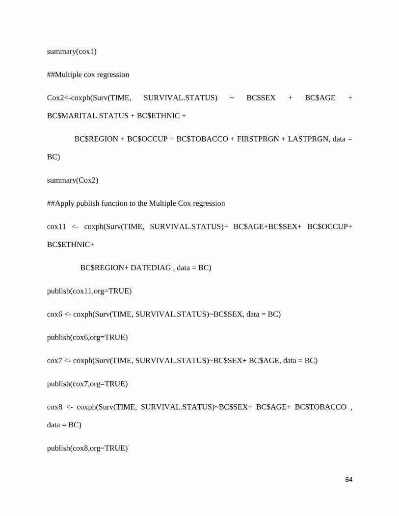
64

summary(cox1)

##Multiple cox regression

Cox2<-coxph(Surv(TIME, SURVIVAL.STATUS) ~ BC$SEX + BC$AGE +

BC$MARITAL.STATUS + BC$ETHNIC +

BC$REGION + BC$OCCUP + BC$TOBACCO + FIRSTPRGN + LASTPRGN, data =

BC)

summary(Cox2)

##Apply publish function to the Multiple Cox regression

cox11 <- coxph(Surv(TIME, SURVIVAL.STATUS)~ BC$AGE+BC$SEX+ BC$OCCUP+

BC$ETHNIC+

BC$REGION+ DATEDIAG , data = BC)

publish(cox11,org=TRUE)

cox6 <- coxph(Surv(TIME, SURVIVAL.STATUS)~BC$SEX, data = BC)


cox7 <- coxph(Surv(TIME, SURVIVAL.STATUS)~BC$SEX+ BC$AGE, data = BC)


cox8 <- coxph(Surv(TIME, SURVIVAL.STATUS)~BC$SEX+ BC$AGE+ BC$TOBACCO ,

data = BC)


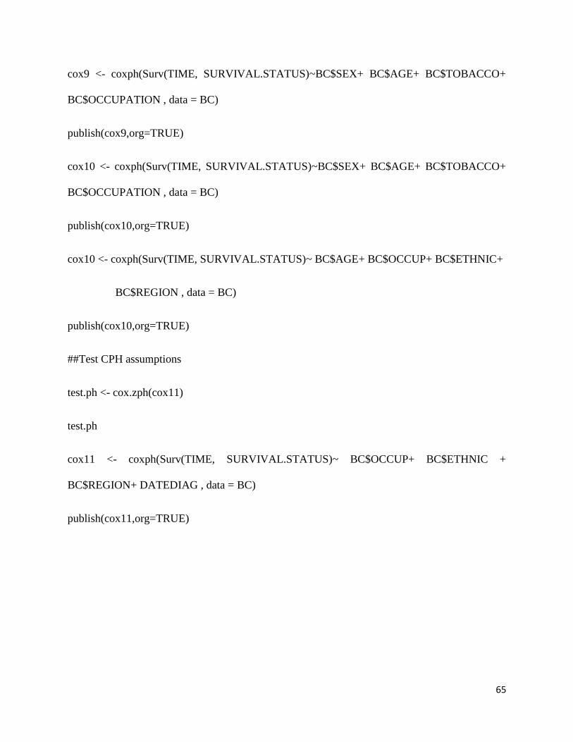
65

cox9 <- coxph(Surv(TIME, SURVIVAL.STATUS)~BC$SEX+ BC$AGE+ BC$TOBACCO+

BC$OCCUPATION , data = BC)


cox10 <- coxph(Surv(TIME, SURVIVAL.STATUS)~BC$SEX+ BC$AGE+ BC$TOBACCO+

BC$OCCUPATION , data = BC)


cox10 <- coxph(Surv(TIME, SURVIVAL.STATUS)~ BC$AGE+ BC$OCCUP+ BC$ETHNIC+

BC$REGION , data = BC)


##Test CPH assumptions

test.ph <- cox.zph(cox11)

test.ph

cox11 <- coxph(Surv(TIME, SURVIVAL.STATUS)~ BC$OCCUP+ BC$ETHNIC +

BC$REGION+ DATEDIAG , data = BC)
