1 / 16

An Application of Linear Algebra to ImageCompression

Paul Dostert

July 2, 2009

Image Compression

2 / 16

There are hundreds of ways to compress images. Some basic ways usesingular value decomposition

Suppose we have an 9 megapixel gray-scale image, which is 3000 × 3000pixels (a 3000 × 3000 matrix). For each pixel, we have some level of blackand white, given by some integer between 0 and 255. Each of these integers(and hence each pixel) requires approximately 1 byte to store, resulting in anapproximately 8.6 Mb image.

A color image usually has three components, a red, a green, and a blue(RGB). EACH of these is represented by a matrix, so storing color imagestakes three times the space (25.8 Mb).

We will look at compressing this image through computing the singular valuedecomposition (SVD).

Singular Value Decomposition (SVD)

3 / 16

Any nonzero real m × n matrix A with rank r > 0 can be factored asA = PΣQT with P an m × r matrix with orthonormal columns,Σ = diag (σ1, . . . , σr) and QT an r × n matrix with orthonormal rows. Thisfactorization is called the singular value decomposition (SVD) .

This is directly related to the spectral theorem which states that if B is asymmetric matrix (BT = B) then we can write B = UΛUT where Λ is adiagonal matrix of eigenvalues and U is an orthonormal matrix ofeigenvectors.

To see the relationship, notice:

AT A = QΣT PT PΣQT = QΣ2QT

AAT = PΣQT QΣT PT = PΣ2PT

These are both spectral decompositions, hence the σi are the positivesquare roots of the eigenvalues of AT A. In the SVD, the matrices arerearranged so that σ1 ≥ σ2 ≥ · · · ≥ σn.

Reducing the SVD

4 / 16

Using the SVD we can write an n × n invertible matrix A as:

A = PΣQT = (p1, p2, . . . ,pn)

σ1 0 · · · 0

0 σ2

. . . 0...

. . .. . .

...0 . . . 0 σn

q1T

q2T

...qn

T

= p1σ1q1T + p2σ2q2

T + · · · + pnσnqnT

Since σ1 ≥ σ2 ≥ · · · ≥ σn the terms piσiqiT with small i contribute most to

the sum, and hence contain the most information about the image. Keepingonly some of these terms may result in a lower image quality, but lowerstorage size. This process is sometimes called Principal ComponentAnalysis (PCA).

Issues in using PCA

5 / 16

● A requires n2 elements. P and Q require n2 elements each and Σrequires n elements. Storing the full SVD then requires 2n2 + n

elements.● Keeping 1 term in the SVD, p1σ11q1

T , requires only 2n + 1 elements.● If we keep k ≈

n

2terms, then storing the reduced SVD and the original

matrix are approximately the same.● The P and Q are normalized (each pi,qi

T has norm 1) so the error inthe reduced SVD is given by only the σ values:

Error = 1 −

∑

k

i=1σi

∑

n

i=1σi

● Color images are often in RGB (red, green, blue) where each color isspecified by 0 to 255. This gives us three matrices. The reduced SVDcan be computed on all three separately or together.

Examples: 1 Term

6 / 16

The following is a 500 × 500 image. The reduced SVD was applied equally toeach color:

Original Using 1 terms

Examples: 3 Terms

7 / 16

The following is a 500 × 500 image. The reduced SVD was applied equally toeach color:

Original Using 3 terms

Examples: 5 Terms

8 / 16

The following is a 500 × 500 image. The reduced SVD was applied equally toeach color:

Original Using 5 terms

Examples: 10 Terms

9 / 16

The following is a 500 × 500 image. The reduced SVD was applied equally toeach color:

Original Using 10 terms

Examples: 20 Terms

10 / 16

The following is a 500 × 500 image. The reduced SVD was applied equally toeach color:

Original Using 20 terms

Examples: 30 Terms

11 / 16

The following is a 500 × 500 image. The reduced SVD was applied equally toeach color:

Original Using 30 terms

Examples: 40 Terms

12 / 16

The following is a 500 × 500 image. The reduced SVD was applied equally toeach color:

Original Using 40 terms

Examples: 50 Terms

13 / 16

The following is a 500 × 500 image. The reduced SVD was applied equally toeach color:

Original Using 50 terms

Examples: 75 Terms

14 / 16

The following is a 500 × 500 image. The reduced SVD was applied equally toeach color:

Original Using 75 terms

Examples: 100 Terms

15 / 16

The following is a 500 × 500 image. The reduced SVD was applied equally toeach color:

Original Using 100 terms

Results & Other Applications

16 / 16

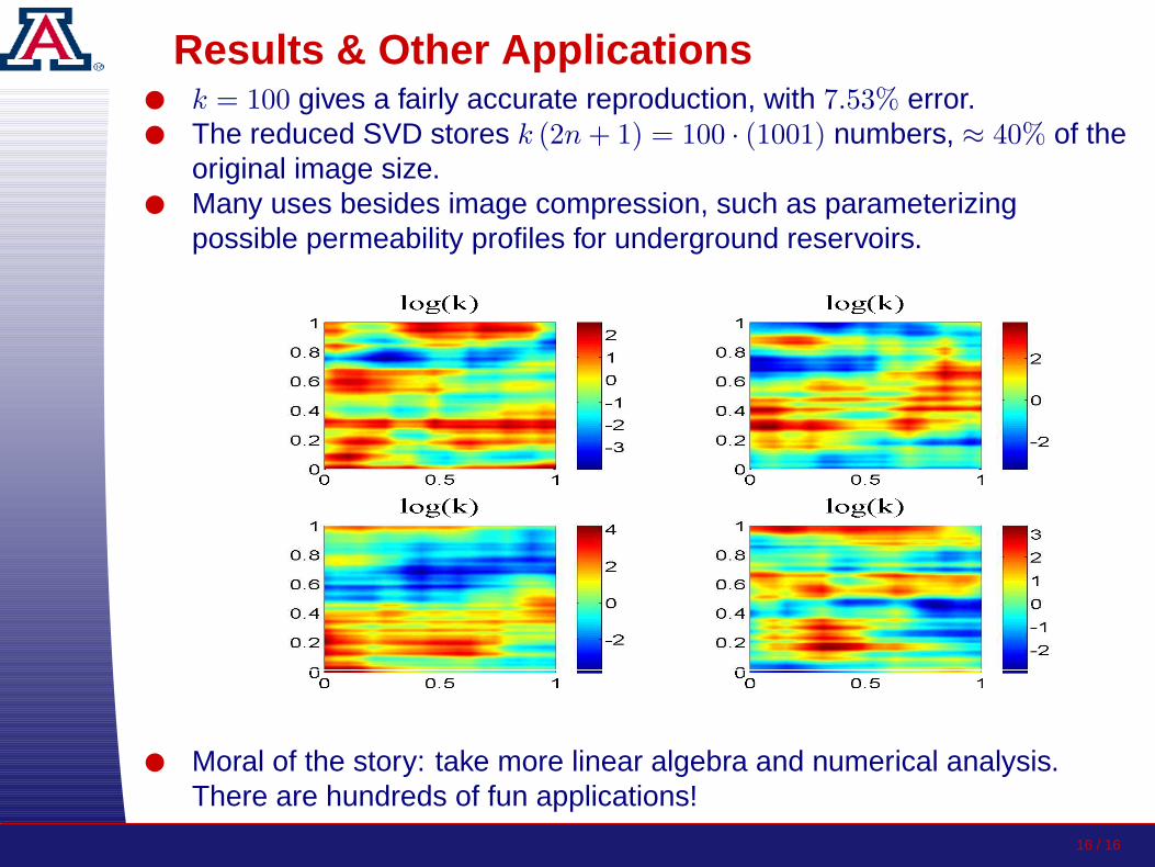
● k = 100 gives a fairly accurate reproduction, with 7.53% error.● The reduced SVD stores k (2n + 1) = 100 · (1001) numbers, ≈ 40% of the

original image size.● Many uses besides image compression, such as parameterizing

possible permeability profiles for underground reservoirs.

● Moral of the story: take more linear algebra and numerical analysis.There are hundreds of fun applications!