An Ant Colony Approach to Forward-Reverse Logistics

An Ant Colony Approach to Forward-Reverse Logistics Network Design Under Demand Certainty Hamed Soleimania,* Mostafa Zohalb

a Assistant Professor, Faculty of Industrial and Mechanical Engineering, Qazvin Branch, Islamic Azad University (IAU), Qazvin, Iran b MSc, Young Researchers and Elite Club, Qazvin Branch, Islamic Azad University, Qazvin, Iran

Received 28 February 2015; Revised 22 September 2015; Accepted 01 October 2015

Abstract

Forward-reverse logistics network has remained a subject of intensive research over the past few years. It is of significant importance to be issued in a supply chain because it affects responsiveness of supply chains. In real world, problems are needed to be formulated. These problems usually involve objectives such as cost, quality, and customers' responsiveness and so on. To this reason, we have studied a single-objective model for an integrated forward/reverse logistics network design. This model includes seven echelons; four echelons in the forward direction and three in the reverse direction. We present an effective algorithm based on ant colony optimization for this NP-hard problems to maximize the benefit. The proposed metaheuristic algorithm is a new approach in the field of closed-loop supply chain network design. Furthermore, the developed model is a three-objective one which regards incomes, costs, and the emissions of CO2. A new approach is utilized in order to integrate three various-dimension objective functions. The performance of the proposed algorithm has been compared utilizing the optimum solutions of the LINGO software. Besides, various instances with small, medium, and large sizes are generated and solved so as to make the evaluation of the algorithm reliable. The obtaining results clearly demonstrate superiority performance of the proposed algorithm.

Keywords: Logistics network, Forward/reverse supply chain, Single-objective, Ant colony optimization.

1. Introduction

Logistics is defined as a process of planning, implementing and controlling the efficient and effective flow and storage of goods, services and information from the beginning point to the point of consumption in order to comply with customer needs (Hugos 2011). Logistics network design is a major strategic decision and assumes a strategic role in effective and efficient supply chain management. That's why it is in dire need to be optimized for effective long-term operation of the entire supply chain (Ramezani et al., 2013).

Logistics network designs are of two types: forward logistics (FL) network and reverse logistics (RL) networks. Due to the separate network design for reverse and forward supply chain objectives, suboptimal designs are created (Pishvaee et al, 2010).Over the past few years, some studies have integrated these two types together. When the reverse logistics network is combined with forward logistics network, a Closed-Loop (C-L) network is created. The advantage of using this network is economizing the costs. To this reason, the use of integrated logistics network is highly recommended.

Some studies have shown that mixed integer programming models (MIP) are the most common models used in this field. These can be ranged from simple single-product uncapacitated facility location models such

as Sung CS and Song SH, 2003 to complex capacitated multi-commodity models such as Tsiakis and Papageorgiou, 2008.Dullaert et al. (2007) who presented an overview of supply chain design models. They indicated that the mixed integer planning models are commonly utilized in this realm. Fleischmann et al. (2001) suggested an integrated approach that has substantial savings in cost compared to the sequential design of both networks. Likewise, Listes and Dekker (2005) proposed a stochastic mixed integer programming model based on a scenario to maximize the profit. Another mixed integer nonlinear programming (MINLP) model for concurrent design of inverse and forward network was offered by Ko and Evan (2007). They used a genetic algorithm developed to solve their model. Halefi and Jolai (2013) proposed a reliability model for their design of an integrated forward/reverse logistics network. Their proposed model was formulated so as to be based on recent robust optimization method in order to protect the network against uncertainty. Therefore, a mixed integer linear programming (MILP) model with complete restrictions was proposed to control network reliability among scenarios. Subramanian et al. (2013) considered a single-period, single-product and multi-echelon of closed

* Corresponding author Email address: [email protected]

Journal of Optimization in Industrial Engineering 22 (2017) 103-114DOI: 10.22094/joie.2017.281

103

network supply chain. They developed MILP using simulated annealing algorithms.

MIP models require enormous computing and information. As a result, when the problem size is large, finding the optimal solution in a reasonable computation time becomes very difficult. Since the majority of the logistics network design problems can be classified as NP-hard, many heuristic and meta-heuristic methods have been developed to solve these models (Pishvaee et al, 2010). Among the methods used to solve the logistics network are: exact method (for small scales), LR method based on heuristic, exact method (continuous), Genetic algorithm (GA), simulated annealing methods (SA), combined heuristic methods, Lagrangian decomposition, Benders decomposition, Genetic based on heuristic and etc.

The present study aimed to illustrate the problem of integrated single-objective, single-product, multi-stage C-L network design including suppliers, manufacturing facilities, distribution centers, collection centers, recycling centers, and disposal centers. Based on the review of literature, the following gaps are observed: 1) There are no papers dealing with three objective

functions (cost, income and emission) simultaneously.

2) Multi-objective models which consider emission as their function are scant.

3) There is virtually no model that considers effective loading percentage of a vehicle

4) This type of model has not been solved by ACO. The rest of the paper is organized as follows: Section

2: an integer linear programming formulation is elaborated and contains description of mathematical model. Section 3 discusses about an efficient solution approach based on ACO for small-scale instances. Eventually, Section 4 concludes the research and suggests some guidelines for future studies.

2. Problem Description

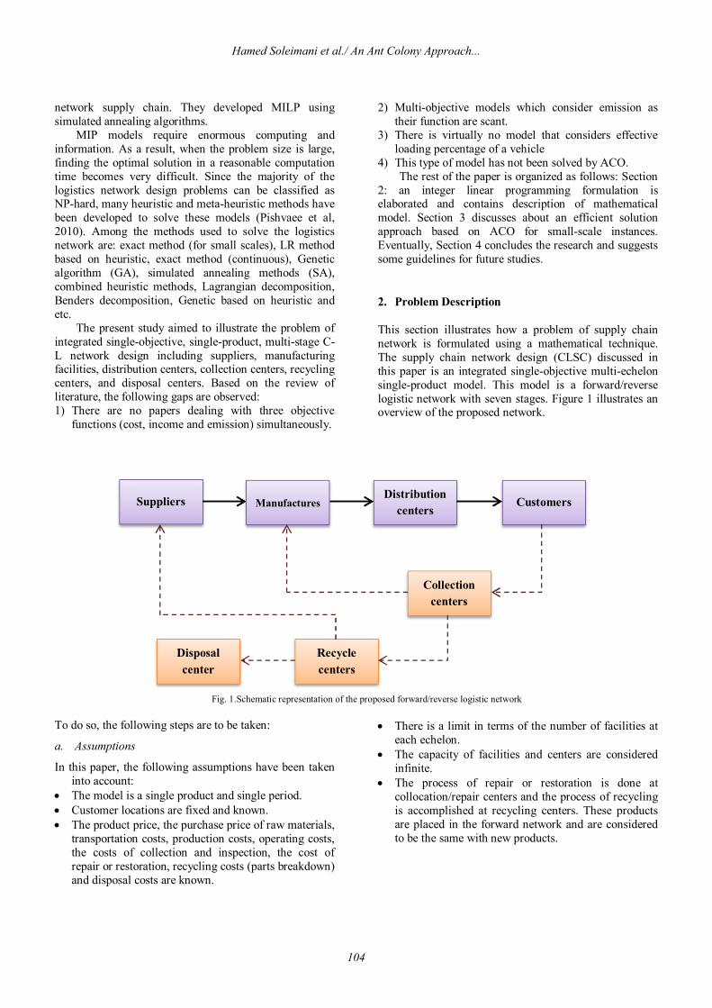
This section illustrates how a problem of supply chain network is formulated using a mathematical technique. The supply chain network design (CLSC) discussed in this paper is an integrated single-objective multi-echelon single-product model. This model is a forward/reverse logistic network with seven stages. Figure 1 illustrates an overview of the proposed network.

Fig. 1.Schematic representation of the proposed forward/reverse logistic network

To do so, the following steps are to be taken:

a. Assumptions

In this paper, the following assumptions have been taken into account:

The model is a single product and single period. Customer locations are fixed and known. The product price, the purchase price of raw materials,

transportation costs, production costs, operating costs, the costs of collection and inspection, the cost of repair or restoration, recycling costs (parts breakdown) and disposal costs are known.

There is a limit in terms of the number of facilities at

each echelon. The capacity of facilities and centers are considered

infinite. The process of repair or restoration is done at

collocation/repair centers and the process of recycling is accomplished at recycling centers. These products are placed in the forward network and are considered to be the same with new products.

Suppliers Manufactures Distribution

centers Customers

Collection centers

Recycle centers

Disposal center

Hamed Soleimani et al./ An Ant Colony Approach...

104

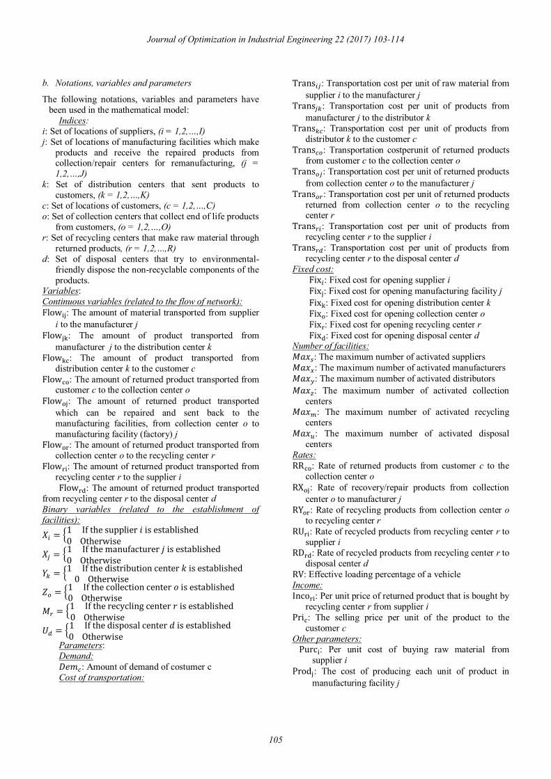
b. Notations, variables and parameters

The following notations, variables and parameters have been used in the mathematical model:

Indices: i: Set of locations of suppliers, (i = 1,2,…,I) j: Set of locations of manufacturing facilities which make

products and receive the repaired products from collection/repair centers for remanufacturing, (j = 1,2,…,J)

k: Set of distribution centers that sent products to customers, (k = 1,2,…,K)

c: Set of locations of customers, (c = 1,2,…,C) o: Set of collection centers that collect end of life products

from customers, (o = 1,2,…,O) r: Set of recycling centers that make raw material through

returned products, (r = 1,2,…,R) d: Set of disposal centers that try to environmental-

friendly dispose the non-recyclable components of the products.

Variables: Continuous variables (related to the flow of network): Flow : The amount of material transported from supplier

i to the manufacturer j Flow : The amount of product transported from

manufacturer j to the distribution center k Flow : The amount of product transported from

distribution center k to the customer c Flow : The amount of returned product transported from

customer c to the collection center o Flow : The amount of returned product transported

which can be repaired and sent back to the manufacturing facilities, from collection center o to manufacturing facility (factory) j

Flow : The amount of returned product transported from collection center o to the recycling center r

Flow : The amount of returned product transported from recycling center r to the supplier i Flow : The amount of returned product transported

from recycling center r to the disposal center d Binary variables (related to the establishment of facilities): 푋 = 1Ifthesupplier푖isestablished

0Otherwise

푋 = 1Ifthemanufacturer푗isestablished0Otherwise

푌 = 1Ifthedistributioncenter푘isestablished0Otherwise

푍 = 1Ifthecollectioncenter표isestablished0Otherwise

푀 = 1Iftherecyclingcenter푟isestablished0Otherwise

푈 = 1Ifthedisposalcenter푑isestablished0Otherwise

Parameters: Demand: 퐷푒푚 : Amount of demand of costumer c Cost of transportation:

Trans : Transportation cost per unit of raw material from supplier i to the manufacturer j

Trans : Transportation cost per unit of products from manufacturer j to the distributor k

Trans : Transportation cost per unit of products from distributor k to the customer c

Trans : Transportation costperunit of returned products from customer c to the collection center o

Trans : Transportation cost per unit of returned products from collection center o to the manufacturer j

Trans : Transportation cost per unit of returned products returned from collection center o to the recycling center r

Trans : Transportation cost per unit of products from recycling center r to the supplier i

Trans : Transportation cost per unit of products from recycling center r to the disposal center d

Fixed cost: Fix : Fixed cost for opening supplier i Fix : Fixed cost for opening manufacturing facility j Fix : Fixed cost for opening distribution center k Fix : Fixed cost for opening collection center o Fix : Fixed cost for opening recycling center r Fix : Fixed cost for opening disposal center d

Number of facilities: 푀푎푥 : The maximum number of activated suppliers 푀푎푥 : The maximum number of activated manufacturers 푀푎푥 : The maximum number of activated distributors 푀푎푥 : The maximum number of activated collection

centers 푀푎푥 : The maximum number of activated recycling

centers 푀푎푥 : The maximum number of activated disposal

centers Rates: RR : Rate of returned products from customer c to the

collection center o RX : Rate of recovery/repair products from collection

center o to manufacturer j RY : Rate of recycling products from collection center o

to recycling center r RU : Rate of recycled products from recycling center r to

supplier i RD : Rate of recycled products from recycling center r to

disposal center d RV: Effective loading percentage of a vehicle Income: Inco : Per unit price of returned product that is bought by

recycling center r from supplier i Pri : The selling price per unit of the product to the

customer c Other parameters: Purc : Per unit cost of buying raw material from

supplier i Prod : The cost of producing each unit of product in

manufacturing facility j

Journal of Optimization in Industrial Engineering 22 (2017) 103-114

105

Dis : Per unit operating cost of product in the distribution center k

Coll : Collection and inspection costs per unit of product in the collection center o

Repa : The cost of repair or restoration of each unit in the collection center o

Brok : Cost of recycling per unit of product at recycling center r

Disp : Per unit disposal cost of non-recyclable product by the disposal center d

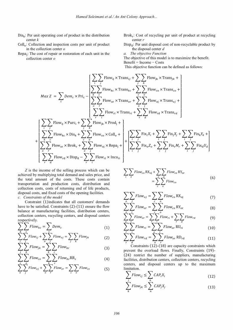
a. The objective Function The objective of this model is to maximize the benefit. Benefit = Income − Costs This objective function can be defined as follows:

푀푎푥푍 = 퐷푒푚 ×Pri −

⎣⎢⎢⎢⎢⎢⎢⎢⎢⎡ Flow ×Trans + Flow ×Trans +

Flow ×Trans + Flow ×Trans +

Flow ×Trans + Flow ×Trans +

Flow ×Trans + Flow ×Trans⎦⎥⎥⎥⎥⎥⎥⎥⎥⎤

+

⎣⎢⎢⎢⎢⎢⎢⎢⎢⎡ Flow ×Purc + Flow ×Prod +

Flow ×Dis + Flow ×Coll +

Flow ×Brok + Flow ×Repa +

Flow ×Disp − Flow × Inco⎦⎥⎥⎥⎥⎥⎥⎥⎥⎤

+

⎣⎢⎢⎢⎡ Fix 푋 + Fix 푋 + Fix 푌 +

Fix 푍 + Fix 푀 + Fix 푈⎦⎥⎥⎥⎤

Z is the income of the selling process which can be

achieved by multiplying total demand and sales price, and the total amount of the costs. These costs contain transportation and production costs, distribution and collection costs, costs of returning end of life products, disposal costs, and fixed costs of the opening facilities. c. Constraints of the model

Constraint (1)indicates that all customers' demands have to be satisfied. Constraints (2)-(11) ensure the flow balance at manufacturing facilities, distribution centers, collection centers, recycling centers, and disposal centers respectively.

퐹푙표푤 = 퐷푒푚 (1)

퐹푙표푤 + 퐹푙표푤 = 퐹푙표푤 (2)

퐹푙표푤 = 퐹푙표푤 (3)

퐹푙표푤 = 퐹푙표푤 RR (4)

퐹푙표푤 + 퐹푙표푤 = 퐹푙표푤 (5)

퐹푙표푤 RX + 퐹푙표푤 RY

= 퐹푙표푤 (6)

퐹푙표푤 = 퐹푙표푤 RX (7)

퐹푙표푤 = 퐹푙표푤 RY (8)

퐹푙표푤 = 퐹푙표푤 + 퐹푙표푤 (9)

퐹푙표푤 = 퐹푙표푤 RU (10)

퐹푙표푤 = 퐹푙표푤 RD (11)

Constraints (12)-(18) are capacity constraints which prevent the overload flows. Finally, Constraints (19)-(24) restrict the number of suppliers, manufacturing facilities, distribution centers, collection centers, recycling centers, and disposal centers up to the maximum limitation.

퐹푙표푤 ≤ 퐶퐴푃푋 (12)



106

퐹푙표푤 ≤ 퐶퐴푃 푌 (14)

퐹푙표푤 + 퐹푙표푤 ≤ 퐶퐴푃 푍 (15)

퐹푙표푤 + 퐹푙표푤 ≤ 퐶퐴푃 푀 (16)

퐹푙표푤 ≤ 퐶퐴푃 푈 (17)


푋 ≤ Max (19)

푋 ≤ Max (20)

푌 ≤ Max (21)

푍 ≤ 푀푎푥 (22)

푀 ≤ 푀푎푥 (23)

푈 ≤ 푀푎푥 (24)

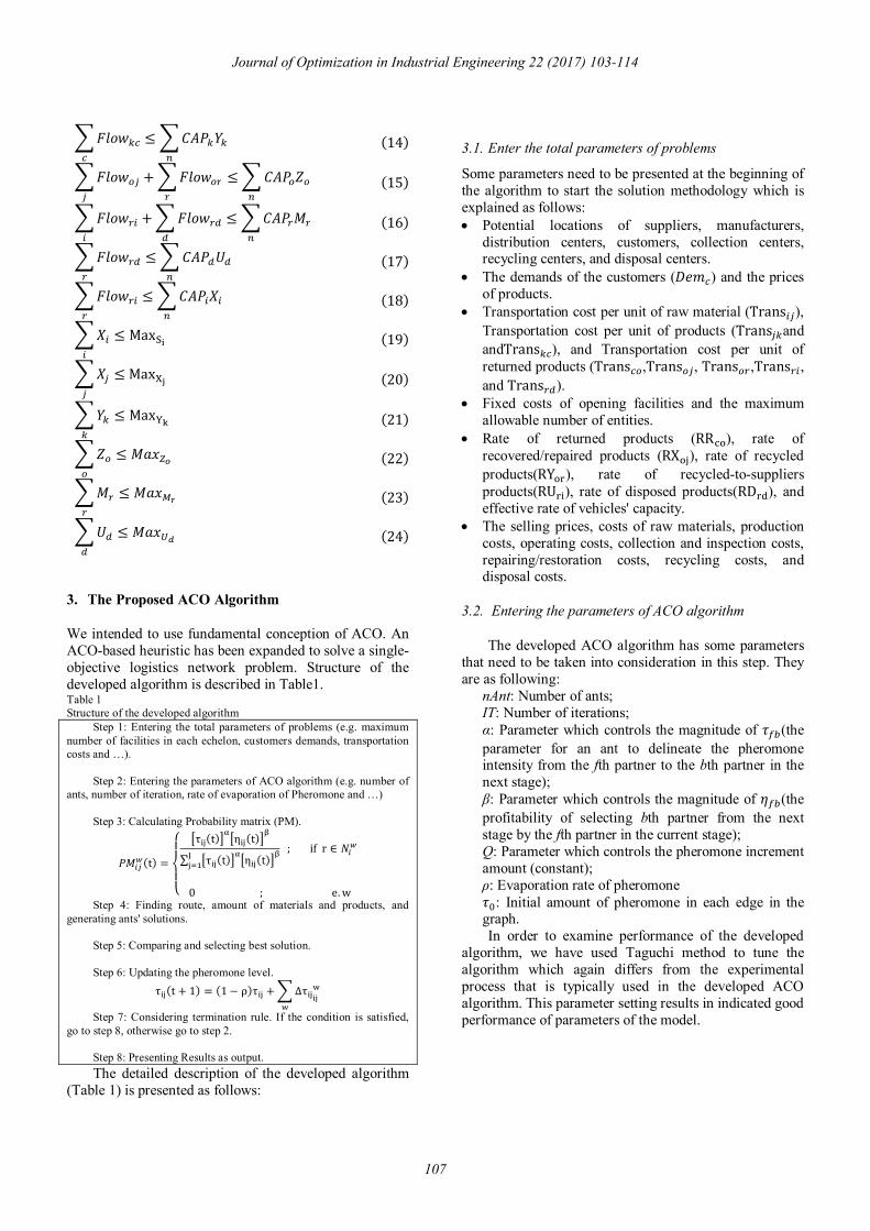
3. The Proposed ACO Algorithm

We intended to use fundamental conception of ACO. An ACO-based heuristic has been expanded to solve a single-objective logistics network problem. Structure of the developed algorithm is described in Table1. Table 1 Structure of the developed algorithm

Step 1: Entering the total parameters of problems (e.g. maximum number of facilities in each echelon, customers demands, transportation costs and …).

Step 2: Entering the parameters of ACO algorithm (e.g. number of

ants, number of iteration, rate of evaporation of Pheromone and …) Step 3: Calculating Probability matrix (PM).

푃푀 (t) =

⎩⎪⎨

⎪⎧ τ (t) η (t)

∑ τ (t) η (t) ; ifr ∈ 푁

0; e. w

Step 4: Finding route, amount of materials and products, and generating ants' solutions.

Step 5: Comparing and selecting best solution. Step 6: Updating the pheromone level.

τ (t + 1) = (1 − ρ)τ + ∆τ

Step 7: Considering termination rule. If the condition is satisfied, go to step 8, otherwise go to step 2.

Step 8: Presenting Results as output. The detailed description of the developed algorithm

(Table 1) is presented as follows:

3.1. Enter the total parameters of problems

Some parameters need to be presented at the beginning of the algorithm to start the solution methodology which is explained as follows: Potential locations of suppliers, manufacturers,

distribution centers, customers, collection centers, recycling centers, and disposal centers.

The demands of the customers (퐷푒푚 ) and the prices of products.

Transportation cost per unit of raw material (Trans ), Transportation cost per unit of products (Trans and andTrans ), and Transportation cost per unit of returned products (Trans ,Trans , Trans ,Trans , and Trans ).

Fixed costs of opening facilities and the maximum allowable number of entities.

Rate of returned products (RR ), rate of recovered/repaired products (RX ), rate of recycled products(RY ), rate of recycled-to-suppliers products(RU ), rate of disposed products(RD ), and effective rate of vehicles' capacity.

The selling prices, costs of raw materials, production costs, operating costs, collection and inspection costs, repairing/restoration costs, recycling costs, and disposal costs.

3.2. Entering the parameters of ACO algorithm

The developed ACO algorithm has some parameters that need to be taken into consideration in this step. They are as following: nAnt: Number of ants; IT: Number of iterations; α: Parameter which controls the magnitude of 휏 (the

parameter for an ant to delineate the pheromone intensity from the fth partner to the bth partner in the next stage);

β: Parameter which controls the magnitude of 휂 (the profitability of selecting bth partner from the next stage by the fth partner in the current stage);

Q: Parameter which controls the pheromone increment amount (constant);

ρ: Evaporation rate of pheromone 휏 : Initial amount of pheromone in each edge in the

graph. In order to examine performance of the developed

algorithm, we have used Taguchi method to tune the algorithm which again differs from the experimental process that is typically used in the developed ACO algorithm. This parameter setting results in indicated good performance of parameters of the model.


107

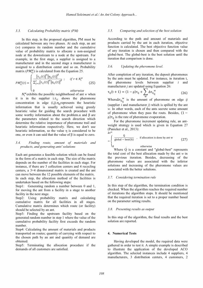
3.3. Calculating Probability matrix (PM)

In this step, in the proposed algorithm, PM must be calculated between any two phases. At each step, an ant (w) compares its random number and the cumulative value of probability matrix to allocate a non-assigned node at the downstream to a node at the upstream. For example, in the first stage, a supplier is assigned to a manufacturer and in the second stage a manufacturer is assigned to a distribution center and so on. Probability matrix (푃푀 ) is calculated from the Equation 25.

푃푀 (푡) =

⎩⎪⎨

⎪⎧ 휏 (푡) 휂 (푡)

∑ 휏 (푡) 휂 (푡); 푖푓푟 ∈ 푁

0; 표푡ℎ푒푟푤푖푠푒

(25)

푁 exhibits the possible neighborhood of ant w when it is in the supplier i.휏 shows the pheromone concentration in edge (i,j).η represents the heuristic information that is usually achieved using greedy heuristic value for guiding the search procedure with some worthy information about the problem.α and β are the parameters related to the search direction which determine the relative importance of pheromone trail and heuristic information respectively. Here, we don't use heuristic information, so the value η is considered to be one, or even it can said that the value of β is equal to zero.

3.4. Finding route, amount of materials and products, and generating ants' solutions

Each ant generates a feasible solution which can be found in the form of a matrix in each step. The size of the matrix depends on the number of the facilities in each stage. For instance, if there are 3 collection centers and 4 recycling centers, a 3×4 dimensional matrix is created and the ant can move between the 12 possible elements of the matrix. In each step, the allocation method of the facilities is undertaken based on the following steps: Step1: Generating random a number between 0 and 1, for moving the ant from a facility in a stage to another facility in the next stage. Step2: Using probability matrix and calculating cumulative matrix for all facilities in all stages. Cumulative matrix determines which route (or facility) should be selected by an ant. Step3: Finding the upstream facility based on the generated random number in step 1 where the value of the cumulative probability facility first exceeds the random number. Step4: Calculating the amount of materials and products transported on routes; quantity of carrying with respect to the chosen path by an ant and quantity of demand are obtained. Step5: Terminating the allocation procedure if the demands of all customers are satisfied.

3.5. Comparing and selection of the best solution

According to the path and amount of materials and products carried by the ant in each iteration, objective function is calculated. The best objective function value of any iteration is chosen and then compared with the global-best. The global-best is the best solution until the iteration that comparison is done.

3.6. Updating the pheromone level.

After completion of any iteration, the deposit pheromones by the ants must be updated. For instance, in iteration t, the pheromone levels between supplier i and manufacturer j are updated using Equation 26: τ (t + 1) = (1 − ρ)τ + ∆τ (26)

Where∆τ is the amount of pheromone on edge ij (supplier i and manufacturer j) which is spilled by the ant w. In other words, each of the ants secrete some amount of pheromone when they pass the routs. Besides, (1 −ρ)τ is the rate of pheromone evaporation.

For the pheromone increment updating rule, an ant-weight strategy is used which is given in Equation 27 (Panicker et al., 2013): ∆τ

=

⎩⎨

⎧Q

global − best(It),ifallocationisdonebyantw

0,otherwise

(27)

Where Q is a constant and "global-best" represents the total cost of the best allocation made by the ant w in the previous iteration. Besides, decreasing of the pheromone values are associated with the inferior solutions and increasing of the pheromone values are associated with the better solutions.

3.7. Considering termination rule

In this step of the algorithm, the termination condition is checked. When the algorithm reaches the required number of iterations the algorithm stops. It should be mentioned that the required iteration is set to a proper number based on the parameter setting results.

3.8. Presenting results as output

In this step of the algorithm, the final results and the best solution are reported.

4. Numerical Tests

Having developed the model, the required data were gathered in order to test it. A simple example is described to illustrate the application of the developed ACO algorithm. The selected instances include 4 suppliers, 4 manufacturers, 3 distribution centers, 4 customers, 2


108

collection centers, 3 recycling centers, and 1 disposal center. The details of the instance parameters are presented in Appendix 1. Customers' demands and the selling price of each product are intended to be equal to 6000 and 1000 respectively. Based on the mentioned phases of the algorithm, the following steps need be taken: Step 1: Entering the total parameters of problems Number of suppliers (푖 = 4), number of manufacturer (푗 = 4), number of distribution centers (푘 = 3), number of customers(푐 = 4), number of collection centers (표 =2), number of recycling center(푟 = 3), number of disposal centers(푑 = 1) are read for the algorithm. The rest of the data is presented in Appendix 1. Step 2: Entering the parameters of ACO algorithm The parameters of the algorithm is determined as the number of ants (n Ant=100), number of iterations (Max IT (IT)=50), α=2, β=5, ρ=0.10, Q=10000, and 휏 = 0.5. Step 3: Probability calculation For the first iteration, according to the Equation 1, probability matrices are obtained. For instance, probability matrices or (푃푀 ) and rd (푃푀 ) are calculated as follows:

(휏 ) = 0.5 0.5 0.50.5 0.5 0.5 → 푃푀 =

[0.5][0.5] + [0.5] + [0.5]

=13

The rest of matrix arrays 푃푀 are calculated as above.

푃푀 =

13

13

13

13

13

13

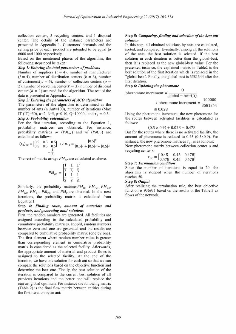
Similarly, the probability matrices푃푀 , 푃푀 , 푃푀 , 푃푀 , 푃푀 , 푃푀 and 푃푀 are obtained. In the next iterations, the probability matrix is calculated from Equation1. Step 4: Finding route, amount of materials and products, and generating ants' solutions First, the random numbers are generated. All facilities are assigned according to the calculated probability and cumulative probability matrices. Indeed, random numbers between zero and one are generated and the results are compared to cumulative probability matrix (one by one). The first element where random number value is greater than corresponding element in cumulative probability matrix is considered as the selected facility. Afterwards, the appropriate amount of material and product flows is assigned to the selected facility. At the end of the iteration, we have one solution for each ant so that we can compare the solutions based on the objective function and determine the best one. Finally, the best solution of the iteration is compared to the current best solution of all previous iterations and the better one will replace the current global optimum. For instance the following matrix (Table 2) is the final flow matrix between entities during the first iteration by an ant:

Step 5: Comparing, finding and selection of the best ant solution In this step, all obtained solutions by ants are calculated, sorted, and compared. Eventually, among all the solutions of the ants, the best solution is selected. If the best solution in each iteration is better than the global-best, then it is replaced as the new global-best value. For the presented instance, the explained matrix in Table2 is the best solution of the first iteration which is replaced in the "global-best". Finally, the global-best is 3581344 after the first iteration. Step 6: Updating the pheromone

pheromoneincrement =Q

global − best(It)

→ pheromoneincrement =1000003581344

≅ 0.028 Using the pheromone increment, the new pheromone for the routes between activated facilities is calculated as follows:

(0.5 × 0.9) + 0.028 = 0.478 But for the routes where there is no activated facility, the amount of pheromone is reduced to 0.45 (0.5×0.9). For instance, the new pheromone matrices 휏 is as follows: New pheromone matrix between collection center o and recycling center r:

휏 = 0.45 0.45 0.4780.478 0.45 0.478

Step 7: Termination condition Since the number of iterations is equal to 20, the algorithm is stopped when the number of iterations reaches 50. Step 8: Output After realizing the termination rule, the best objective function is 936931 based on the results of the Table 3 as flows of the network.


109

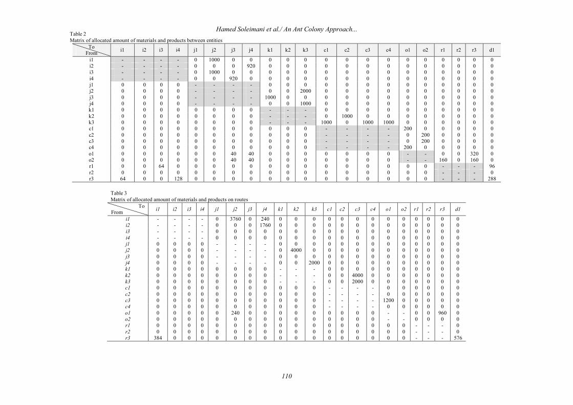
Table 2 Matrix of allocated amount of materials and products between entities

To From i1 i2 i3 i4 j1 j2 j3 j4 k1 k2 k3 c1 c2 c3 c4 o1 o2 r1 r2 r3 d1

i1 - - - - 0 1000 0 0 0 0 0 0 0 0 0 0 0 0 0 0 0 i2 - - - - 0 0 0 920 0 0 0 0 0 0 0 0 0 0 0 0 0 i3 - - - - 0 1000 0 0 0 0 0 0 0 0 0 0 0 0 0 0 0 i4 - - - - 0 0 920 0 0 0 0 0 0 0 0 0 0 0 0 0 0 j1 0 0 0 0 - - - - 0 0 0 0 0 0 0 0 0 0 0 0 0 j2 0 0 0 0 - - - - 0 0 2000 0 0 0 0 0 0 0 0 0 0 j3 0 0 0 0 - - - - 1000 0 0 0 0 0 0 0 0 0 0 0 0 j4 0 0 0 0 - - - - 0 0 1000 0 0 0 0 0 0 0 0 0 0 k1 0 0 0 0 0 0 0 0 - - - 0 0 0 0 0 0 0 0 0 0 k2 0 0 0 0 0 0 0 0 - - - 0 1000 0 0 0 0 0 0 0 0 k3 0 0 0 0 0 0 0 0 - - - 1000 0 1000 1000 0 0 0 0 0 0 c1 0 0 0 0 0 0 0 0 0 0 0 - - - - 200 0 0 0 0 0 c2 0 0 0 0 0 0 0 0 0 0 0 - - - - 0 200 0 0 0 0 c3 0 0 0 0 0 0 0 0 0 0 0 - - - - 0 200 0 0 0 0 c4 0 0 0 0 0 0 0 0 0 0 0 - - - - 200 0 0 0 0 0 o1 0 0 0 0 0 0 40 40 0 0 0 0 0 0 0 - - 0 0 320 0 o2 0 0 0 0 0 0 40 40 0 0 0 0 0 0 0 - - 160 0 160 0 r1 0 0 64 0 0 0 0 0 0 0 0 0 0 0 0 0 0 - - - 96 r2 0 0 0 0 0 0 0 0 0 0 0 0 0 0 0 0 0 - - - 0 r3 64 0 0 128 0 0 0 0 0 0 0 0 0 0 0 0 0 - - - 288

Table 3 Matrix of allocated amount of materials and products on routes

To From i1 i2 i3 i4 j1 j2 j3 j4 k1 k2 k3 c1 c2 c3 c4 o1 o2 r1 r2 r3 d1

i1 - - - - 0 3760 0 240 0 0 0 0 0 0 0 0 0 0 0 0 0 i2 - - - - 0 0 0 1760 0 0 0 0 0 0 0 0 0 0 0 0 0 i3 - - - - 0 0 0 0 0 0 0 0 0 0 0 0 0 0 0 0 0 i4 - - - - 0 0 0 0 0 0 0 0 0 0 0 0 0 0 0 0 0 j1 0 0 0 0 - - - - 0 0 0 0 0 0 0 0 0 0 0 0 0 j2 0 0 0 0 - - - - 0 4000 0 0 0 0 0 0 0 0 0 0 0 j3 0 0 0 0 - - - - 0 0 0 0 0 0 0 0 0 0 0 0 0 j4 0 0 0 0 - - - - 0 0 2000 0 0 0 0 0 0 0 0 0 0 k1 0 0 0 0 0 0 0 0 - - - 0 0 0 0 0 0 0 0 0 0 k2 0 0 0 0 0 0 0 0 - - - 0 0 4000 0 0 0 0 0 0 0 k3 0 0 0 0 0 0 0 0 - - - 0 0 2000 0 0 0 0 0 0 0 c1 0 0 0 0 0 0 0 0 0 0 0 - - - - 0 0 0 0 0 0 c2 0 0 0 0 0 0 0 0 0 0 0 - - - - 0 0 0 0 0 0 c3 0 0 0 0 0 0 0 0 0 0 0 - - - - 1200 0 0 0 0 0 c4 0 0 0 0 0 0 0 0 0 0 0 - - - - 0 0 0 0 0 0 o1 0 0 0 0 0 240 0 0 0 0 0 0 0 0 0 - - 0 0 960 0 o2 0 0 0 0 0 0 0 0 0 0 0 0 0 0 0 - - 0 0 0 0 r1 0 0 0 0 0 0 0 0 0 0 0 0 0 0 0 0 0 - - - 0 r2 0 0 0 0 0 0 0 0 0 0 0 0 0 0 0 0 0 - - - 0 r3 384 0 0 0 0 0 0 0 0 0 0 0 0 0 0 0 0 - - - 576


110

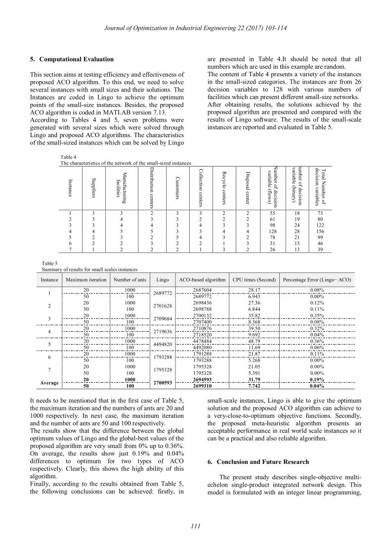
5. Computational Evaluation

This section aims at testing efficiency and effectiveness of proposed ACO algorithm. To this end, we need to solve several instances with small sizes and their solutions. The Instances are coded in Lingo to achieve the optimum points of the small-size instances. Besides, the proposed ACO algorithm is coded in MATLAB version 7.13. According to Tables 4 and 5, seven problems were generated with several sizes which were solved through Lingo and proposed ACO algorithms. The characteristics of the small-sized instances which can be solved by Lingo

are presented in Table 4.It should be noted that all numbers which are used in this example are random. The content of Table 4 presents a variety of the instances in the small-sized categories. The instances are from 26 decision variables to 128 with various numbers of facilities which can present different small-size networks. After obtaining results, the solutions achieved by the proposed algorithm are presented and compared with the results of Lingo software. The results of the small-scale instances are reported and evaluated in Table 5.

Table 4 The characteristics of the network of the small-sized instances

Instance

Suppliers

Manufacturing facilities

Distribution centers

Custom

ers

Collection centers

Recycle centers

Disposal center

Num

ber of decision variable (flow

s)

Num

ber of decision variable (binary)

Total Num

ber of decision variables

1 3 3 2 3 3 2 2 55 18 73 2 3 4 3 3 2 2 2 61 19 80 3 3 4 4 3 4 3 3 98 24 122 4 4 5 5 3 3 4 4 128 28 156 5 2 3 2 5 4 3 2 78 21 99 6 2 2 3 2 2 1 3 31 15 46 7 1 2 2 2 1 3 2 26 13 39

Table 5 Summary of results for small scales instances Instance Maximum iteration Number of ants Lingo ACO-based algorithm CPU times (Second) Percentage Error (Lingo− ACO)

1 20 1000 2689772 2687604 28.17 0.08% 50 100 2689772 6.943 0.00%

2 20 1000 2701628 2698436 27.36 0.12% 50 100 2698788 6.844 0.11%

3 20 1000 2709684 2700132 35.82 0.35% 50 100 2707400 8.368 0.08%

4 20 1000 2719636 2710876 39.50 0.32% 50 100 2718520 9.692 0.04%

5 20 1000 4494820 4478484 48.79 0.36% 50 100 4492080 11.69 0.06%

6 20 1000 1793288 1791288 21.87 0.11% 50 100 1793288 5.268 0.00%

7 20 1000 1795328 1795328 21.05 0.00% 50 100 1795328 5.391 0.00%

Average 20 1000 2700593 2694593 31.79 0.19% 50 100 2699310 7.742 0.04%

It needs to be mentioned that in the first case of Table 5, the maximum iteration and the numbers of ants are 20 and 1000 respectively. In next case, the maximum iteration and the number of ants are 50 and 100 respectively. The results show that the difference between the global optimum values of Lingo and the global-best values of the proposed algorithm are very small from 0% up to 0.36%. On average, the results show just 0.19% and 0.04% differences to optimum for two types of ACO respectively. Clearly, this shows the high ability of this algorithm. Finally, according to the results obtained from Table 5, the following conclusions can be achieved: firstly, in

small-scale instances, Lingo is able to give the optimum solution and the proposed ACO algorithm can achieve to a very-close-to-optimum objective functions. Secondly, the proposed meta-heuristic algorithm presents an acceptable performance in real world scale instances so it can be a practical and also reliable algorithm.

6. Conclusion and Future Research

The present study describes single-objective multi-echelon single-product integrated network design. This model is formulated with an integer linear programming,


111

and using lingo software, the mathematical model is solved with branch and bound method. While these problems are NP-hard, we use heuristic and Meta-heuristic algorithms for solving them. Thus, we introduced a new solving methodology for a multi-stage closed-loop logistics network model based on the ant colony optimization. For this purpose, the model is coded by Lingo 11 to achieve the global optimum and then the ACO-based algorithm is coded by MATLAB 7.13 software. To evaluate performance of the proposed algorithm, 7 instances with small sizes were developed the performance of the ACO algorithm was compared to the optimal solutions obtained by Lingo. The differences of two proposed types of ACO with the optimum points of Lingo are just 0.19% and 0.04% which are completely acceptable.

Based on the limitations and assumptions of the current study, some future research can be suggested. In this study, the model is a single product which can be developed to a multi-product network. Likewise, the single-period can be developed. In this paper, all parameters are considered deterministic, whereas in the real world some parameters are stochastic such as demand and price. Moreover, the proposed green supply chain can be extended to a more complex multi-layered model. Furthermore, performance investigation of the solution method with other optimizer, e.g., Non-dominated Sorting Genetic Algorithm and Multi Objective Simulated is recommended. Finally, this algorithm can be used for other optimization problems in the field of CLSC. Another opportunity for research is to consider the other optimization objectives, such as robustness or responsiveness, or even multi-objective cases.

References

Dullaert W., Braysy O., Goetschalckx M., & Raa B. (2007), Supply chain (re)design: support for managerial and policy decisions, European Journal of Transport and Infrastructure Research, 7(2), 73–9.

Fleischmann M., Beullens P., Bloemhof-Ruwaardj. M., & Vanwassenhove. (2001). The impact of product recovery on logistics network design. Production and Operations Management. 10(2). P 156-73

Hatefi S.M., & Jolai F. (2013). Robust and reliable forward–reverse logistics network design under demand uncertainty and facility disruptions. Applied Mathematical Modelling. 38(9), 2630–2647

Hugos, M. H. (2011). Essentials of supply chain management. Third edition, Hoboken, NJ:John Wiley & Sons (64).

Ko H.J., & Evans G.W. (2007). A genetic-based heuristic for the dynamic integrated forward/reverse logistics network for 3PLS. Computers and Operations Research, 34(2). 346-366

Listes O., & Dekker R. (2005). A stochastic approach to a case study for product recovery network design. European Journal of Operation Research. 160(1). 268-287

Panicker V.V., Vanga R., & Sridharan R. (2013).Ant colony optimisation algorithm for distribution-allocation problem in a two-stage supply chain with a fixed transportation charge.

International Journal of Production Research. 51(3). 698–717

Pishvaee M.S., ZanjiraniFarahani R., & Dullaert W. (2010). A memetic algorithm for bi-objective integrated forward/reverse logistics network design. Computers and Operations Research. 37(6). 1100–1112

Ramezani M., Bashiri M., & Tavakkoli-Moghaddam R. (2013). A new multi-objective stochastic model for a forward/reverse logistic network design with responsiveness and quality level. Applied Mathematical Modeling. 37(1–2). 328-344

Subramanian P., Ramkumar N., Narendran T.T., & Ganesh K. (2013). PRISM: PRIority based simulated annealing for a closed loop supply chain network design problem. Applied Soft Computing. 13(2). 1121-1135

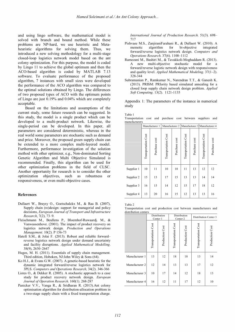
Appendix 1: The parameters of the instance in numerical study

Table 1 Transportation cost and purchase cost between suppliers and manufacturers

Manufacturer 1 Manufacturer 2 Manufacturer 3 Manufacturer 4

Tran

spor

tatio

n C

ost

Purc

hase

cos

t

Tran

spor

tatio

n C

ost

Purc

hase

cos

t

Tran

spor

tatio

n C

ost

Purc

hase

cos

t

Tran

spor

tatio

n C

ost

Purc

hase

cos

t

Supplier 1 10 11 10 10 11 13 12 12

Supplier 2 15 13 17 15 13 13 14 14

Supplier 3 16 15 14 12 15 17 18 12

Supplier 4 13 20 16 15 12 13 13 16

Table 2 Transportation cost and production cost between manufacturers and distribution centers

Distribution Center 1

Distribution Center 2 Distribution Center 3

Tran

spor

tatio

n C

ost

Prod

uctio

n C

ost

Tran

spor

tatio

n C

ost

Prod

uctio

n C

ost

Tran

spor

tatio

n C

ost

Prod

uctio

n C

ost

Manufacturer 1 13 12 18 18 13 14

Manufacturer 2 12 14 13 13 17 12

Manufacturer 3 10 17 14 12 18 13

Manufacturer 4 16 12 11 17 12 10


112

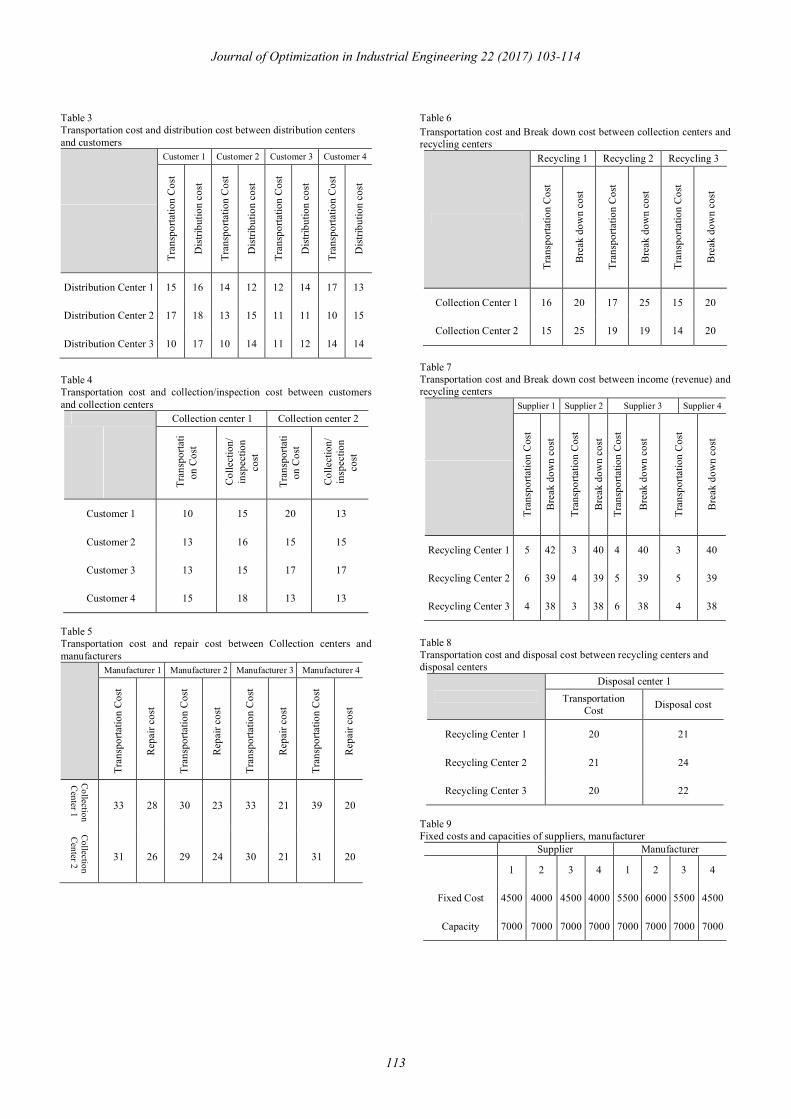
Table 3 Transportation cost and distribution cost between distribution centers and customers

Customer 1 Customer 2 Customer 3 Customer 4 Tr

ansp

orta

tion

Cos

t

Dis

tribu

tion

cost

Tran

spor

tatio

n C

ost

Dis

tribu

tion

cost

Tran

spor

tatio

n C

ost

Dis

tribu

tion

cost

Tran

spor

tatio

n C

ost

Dis

tribu

tion

cost

Distribution Center 1 15 16 14 12 12 14 17 13



Table 4 Transportation cost and collection/inspection cost between customers and collection centers

Collection center 1 Collection center 2

Tran

spor

tati

on C

ost

Col

lect

ion/

in

spec

tion

cost

Tran

spor

tati

on C

ost

Col

lect

ion/

in

spec

tion

cost

Customer 1 10 15 20 13

Customer 2 13 16 15 15

Customer 3 13 15 17 17

Customer 4 15 18 13 13

Table 5 Transportation cost and repair cost between Collection centers and manufacturers

Manufacturer 1 Manufacturer 2 Manufacturer 3 Manufacturer 4

Tran

spor

tatio

n C

ost

Rep

air c

ost

Tran

spor

tatio

n C

ost

Rep

air c

ost

Tran

spor

tatio

n C

ost

Rep

air c

ost

Tran

spor

tatio

n C

ost

Rep

air c

ost

Collection Center 1

33 28 30 23 33 21 39 20

Collection Center 2

31 26 29 24 30 21 31 20

Table 6 Transportation cost and Break down cost between collection centers and recycling centers

Recycling 1 Recycling 2 Recycling 3

Tran

spor

tatio

n C

ost

Bre

ak d

own

cost

Tran

spor

tatio

n C

ost

Bre

ak d

own

cost

Tran

spor

tatio

n C

ost

Bre

ak d

own

cost

Collection Center 1 16 20 17 25 15 20

Collection Center 2 15 25 19 19 14 20

Table 7 Transportation cost and Break down cost between income (revenue) and recycling centers

Supplier 1 Supplier 2 Supplier 3 Supplier 4

Tran

spor

tatio

n C

ost

Bre

ak d

own

cost

Tran

spor

tatio

n C

ost

Bre

ak d

own

cost

Tran

spor

tatio

n C

ost

Bre

ak d

own

cost

Tran

spor

tatio

n C

ost

Bre

ak d

own

cost

Recycling Center 1 5 42 3 40 4 40 3 40



Table 8 Transportation cost and disposal cost between recycling centers and disposal centers

Disposal center 1

Transportation Cost Disposal cost

Recycling Center 1 20 21



Table 9 Fixed costs and capacities of suppliers, manufacturer

Supplier Manufacturer

1 2 3 4 1 2 3 4

Fixed Cost 4500 4000 4500 4000 5500 6000 5500 4500

Capacity 7000 7000 7000 7000 7000 7000 7000 7000


113

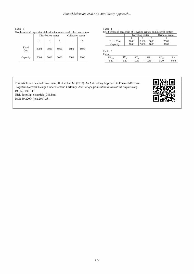
Table 10 Fixed costs and capacities of distribution centers and collection centers

Distribution center Collection center

1 2 3 1 2

Fixed Cost 3000 7000 5000 3500 3500

Capacity 7000 7000 7000 7000 7000

Table 11 Fixed costs and capacities of recycling centers and disposal centers

Recycling center Disposal center 1 2 3 1

Fixed Cost 2000 2500 3000 2500 Capacity 7000 7000 7000 7000

Table 12 Rates

RR RX

RY RU RD RV 0.20 0.20 0.80 0.80 0.20 0.90

This article can be cited: Soleimani, H. &Zohal, M. (2017). An Ant Colony Approach to Forward-Reverse Logistics Network Design Under Demand Certainty. Journal of Optimization in Industrial Engineering. 10 (22), 103-114. URL: http://qjie.ir/article_281.html DOI: 10.22094/joie.2017.281


114

Documents

An Ant Colony Approach to Forward-Reverse Logistics