Embed Size (px)
Citation preview
ISSN: 2281-1346
Department of Economics and Management
DEM Working Paper Series
An anatomy of the Level 3 fair-value hierarchy discount
Emanuel Bagna
(Università di Pavia)
Giuseppe Di Martino
(Università Bocconi, Milano)
Davide Rossi
(Università Bocconi, Milano)
# 65 (01-14)
Via San Felice, 5
I-27100 Pavia
http://epmq.unipv.eu/site/home.html
January 2014
1
An anatomy of the Level 3 fair-value hierarchy discount
Emanuel Bagna*
Giuseppe Di Martino**
Davide Rossi***
Abstract
We use an integrated approach to analyze the reasons behind the discount on the balance-sheet fair
value of illiquid financial instruments held by European banks and classified into the Level 3 Fair
Value hierarchy under IFRS 7. We believe that the potential sources of misalignment are 1) the lack
of disclosure, 2) earnings management, and 3) the lack of liquidity. We show that the discount
implicit in market values is linked to the lack of mandatory additional disclosure required by IFRS 7
and that this result support the strong enforcement activity made by national authorities. We also
show that financial markets penalize banks that transfer assets from other fair-value hierarchy levels
and that the penalty is due both to the instruments’ drop in liquidity and the opacity of the transfers.
Keywords: Fair value hierarchy, Level 3, liquidity discount, financial instruments,
JEL Classification: G120, G150, G180, G210, G280, G320, G380
This paper is part of "PRIN MISURA" research project
* Contact author, Department of Economics and Management, University of Pavia. [email protected]
** Accounting Department, Bocconi University, [email protected]
*** Accounting Department, Bocconi University, [email protected]
2
Introduction
This study tests, through an integrated approach, the extent to which European banks’ market prices
reflect the balance sheet value of financial instruments estimated at fair value. Previous research on
US samples documents the value relevance of fair-value hierarchy information, showing that, in
case of Level 3 financial instruments (i.e., less liquid assets), only a fraction of the balance sheet
value is captured by market prices. Our research confirms that, for European banks, Level 3 net
assets are priced at discount. Our model also allows for the incorporation of incremental
information—such as the choice to disclose and the content of that disclosure—to uncover the
reasons for the differences between balance sheet and market value. Potential sources of the
difference are as follows.
i) Earnings management: Level 3 valuations make use of unobservable inputs, i.e.,
internally sourced estimates, characterized by a high level of subjectivity. The degree of
variation in inputs could allow managers to manipulate these inputs to overvalue
financial instruments classified within Level 3. Supporting this argument, the ratio of
Level 3 net assets over tangible book value was very high at the end of 2008, about 48%
of tangible book value, and Dexia bank, which was bailed out by the Belgian
government during the financial crisis, had Level 3 assets of about 12 times tangible
book value. It is clear that the market considered just a fraction of the fair value derived
from management estimates, thus balancing out managers’ choice of inputs.
ii) Lack of liquidity: managers might not include a liquidity discount in fair value estimates,
while the market typically considers the lower liquidity of financial instruments (either
at the single activity or portfolio level).
iii) Disclosure opacity: opacity in disclosure of methods for estimating fair value and annual
changes might drive the market to incorporate only a fraction of the fair value estimate.
Lambert, Leuz and Verecchia (2007) demonstrate that the amount and quality of financial statement
disclosure has a significant effect on companies’ beta. Since beta is a determinant of market prices,
we expect that the level of disclosure contributes to the market value of a company. Consistent with
this theory, we expect that the discount attributed to Level 3 net assets is strictly linked to the level
of disclosure.
In Europe, fair-value disclosure discipline under IFRS accounting has increased, with a two-year
delay after the insights that US GAAP introduced in 2007. In March 2009, against the background
3
of high volatility and lack of liquidity following the Lehman Brothers default, the International
Accounting Standard Board (IASB) published an amended version of IFRS 7, requiring additional
disclosure for financial instruments estimated at fair value. That was a response to the market’s
demand for greater transparency about the trading activities of financial institutions; investors
wanted to know the amount of illiquid assets banks were holding in their portfolios, mainly as
related to subprime lending. Thus, by amending ―IFRS 7 Financial Instruments: Disclosures,‖ the
IASB required financial institutions to declare the amount of assets that had been estimated at fair
value through a strict three-layer hierarchy, almost identical to the one already adopted by SFAS
157 in the US. Level 1 mark-to-market estimates are directly derived from market prices. Level 2
mark-to-matrix estimates are indirectly related to market prices. And Level 3 mark-to-model
estimates are modeled by using unobservable inputs.
Additional disclosure, required by amended IFRS 7, followed users requests for better information
on the nuances of Level 3 financial instruments. European market regulators through ESMA
(European Securities and Markets Authority1) had strongly urged companies to completely fulfill
additional disclosure requirements of IFRS 7. National authorities behaved similarly, following
supra-national directions, by publishing documents designed to enforce adoption of IFRS 7 and
focusing, in particular, on disclosure. As an example, in March 2010 in Italy, three major
authorities—CONSOB (the market regulator), Banca d’Italia (the bank regulator), and ISVAP (the
insurance regulator2)— jointly published a document that standardized the format for disclosure of
changes in Level 3 under IFRS 7, requiring immediate adoption.3 From the outset, the relevance of
additional disclosure seemed high. We believe that the actual IFRS 7 disclosure framework allows a
full understanding of the reasons for the discount for Level 3 activities. In fact, information
disclosed might produce a priori the following expectations.
1. The analysis of the level of net profit generated by Level 3 activities could lead to the
detection of earnings management.
1 ESMA is an independent EU authority that contributes to safeguarding the stability of the European Union's financial
system by ensuring the integrity, transparency, efficiency, and orderly functioning of securities markets, as well as
enhancing investor protection. In particular, ESMA fosters supervisory convergence both among securities regulators
and across financial sectors by working closely with the other European supervisory authorities competent in the field
of banking (EBA) and insurance and occupational pensions (EIOPA). 2 In January 2013, Isvap (an institution for the security of private and of social interest insurances) was dissolved. All its
powers were transferred to the newly established IVASS (an institution for the security of insurance companies). 3 Fiscal years 2009 and 2010, ―Disclosure in financial reports on asset impairment tests, financial debt contract clauses,
debt restructuring and fair value hierarchy,‖ Bank of Italy-Consob-Isvap Document no. 4 of 3, March 2010, Bank of
Italy, Consob and Isvap coordination forum on applying IAS/IFRS, downloadable at
http://www.bancaditalia.it/vigilanza/att-vigilanza/accordi-altre-autorita/accordi-aut-
italiane/tavolo_coordinamento/fin_reports09_10.pdf
4
2. Detection of transfers from Levels 1 and 2 to Level 3 should allow the quantification of the
drop in liquidity of transferred net assets (financial instruments that were quoted but are not
anymore) or the identification of the possibility of hiding unrealized future losses by
transferring activities to a more opaque category. The detection of a positive market reaction
after a transfer from Level 3 to Levels 1 and 2 (i.e., greater liquidity) should support the
liquidity hypothesis.
3. The amount of net investment can give users an idea about portfolio management policy. A
strong portfolio turnover would raise questions about the estimated fair value of assets. (For
example, why should a commercial bank buy illiquid assets?)
Equipped with this information, investors not only should be able to draw a picture of the amount of
opaque, illiquid instruments on the balance sheet but also should be able to trace the dynamics of
those assets, gaining insight to portfolio management policies and the potential opportunistic use of
financial estimates on the balance sheet. The availability of this information should allow the
market to derive its own fair value estimate for trading activities, thus adjusting balance sheet
tangible book values—which implicitly incorporates a full fair value estimate—in the bank’s
valuation.
If the market gathered this information and used it in formulating prices, we would expect to find a
significant incremental effect within the cross section of banks analyzed by using the same
integrated framework adopted for testing the fair-value hierarchy in the European sample.
Our research focused on a sample of European banks during the period between 2008 and 2012.
Following the Ohlson residual-income model, we tested fair value estimates of Level 1 to 3
financial instruments recorded in financial statements, capturing a discount on Level 3 net assets of
about 11%. The discount on European banks is not aligned with the discount found in research
focused on US financial institutions. Notably, European banks were required to apply the fair-value
hierarchy two years later than US banks. Oddly enough, during 2009, European banks halved their
Level 3 financial instruments, mainly through divestments and consequent losses. Within the sub-
sample of banks that immediately (2009) disclosed the fair-value hierarchy and related changes, the
ratio of Level 3 assets to tangible book value was about 21.7% in 2009. The same ratio was a lot
higher in 2008, about 48.1%. It is likely that reductions in Level 3 assets have been a consequence
of amended IFRS 7 requirements and related enforcement by market authorities, and this probably
affected the size of the discount implicit in Level 3 financial instruments. Our analysis shows that
the discount is due to information risk and potential earnings management.
5
a) Information risk: banks that do not provide required disclosure on changes in Level 3 assets
show a discount on Level 3 financial instruments that is completely recovered for banks that
do provide disclosure, all else equal. In other words, the market reflects information risk
through a lower price for the bank. The presence of a Level 3 discount supports IASB’s
efforts to produce higher quality financial statement standards and regulators’ attempts—in
particular those by ESMA—to make a priority of enforcement of disclosures of Level 3
financial instruments. ESMA enforcement led to an increase in the percentage of banks
disclosing the fair-value hierarchy and change in fair value Level 3 from 72.9% on
31.12.2009 to 94.1% on 31.12.2012.
b) Potential earnings management and the liquidity hypothesis:
a) Banks that transfer a significant amount of Level 1 and 2 assets into Level 3 receive, on
equal terms, lower valuations by the market. The discount is directly linked to the amount of
assets transferred, and it is, from a theoretical standpoint, perfectly in line both with a
liquidity discount applied on financial instruments that are not traded (and not already
captured in fair value estimates) and with a broader discount due to potential fair value
manipulation. Banks’ management might be induced to transfer financial instruments
downward in the fair-value hierarchy to manage the valuation process (e.g., to avoid losses);
b) Banks that transfer significant amount of Level 3 assets upward receive, in general, a
lower valuation by the market. Genuine transfer upward should be accompanied by an
increase recover in the financial instrument’s liquidity, which should in theory lead to a
higher valuation. Empirical evidence strongly supports the presence of a discount on the
entire transfer of a block of assets from and to Level 3. However, we find evidence that
small transfers are positively correlated with market prices, while big transfers retain a large
discount. Those results support the hypothesis that large transfers within the fair-value
hierarchy are discounted from market prices because of the possibility that management
managed earnings.
2. Accounting rules on the fair-value hierarchy under IFRS 7 amended
An amendment to IFRS 7 introduces the fair-value hierarchy (section 27A), a three-layer structure
in which financial instruments must be classified. The levels of the valuation hierarchy are as
follows.
Level 1: “quoted prices (unadjusted) in active markets for identical assets or liabilities”
(c.d. mark-to-market). The classification of a financial instrument within Level 1 is
linked to the existence of two requirements. The first is the presence of an ―active
6
market,‖ as previously defined in IAS 39-AG714 or, equivalently, in IFRS 13: ―IFRS 13
defines an active market as a market in which transactions for the asset or liability take
place with sufficient frequency and volume to provide pricing.‖ The concept of active
market concerns the individual financial instrument being valued and not the market in
which it is quoted. Therefore the fact that a financial instrument is quoted on a regulated
market is not, in itself, a sufficient condition for the instrument to be defined as quoted
in an active market. The second requirement is represented by the term ―unadjusted,‖
i.e., the quote must not be adjusted.
Level 2: “inputs other than quoted prices included within Level 1 that are observable for
the asset or liability, either directly (i.e., as prices) or indirectly (i.e., derived from prices)”
(c.d. mark-to-matrix). The estimate of the fair value of Level 2 (as well as Level 3) requires
the use of valuation techniques. If the valuation technique is based on observable inputs that
do not require adjustment based on unobservable inputs, the financial instrument is
classified in Level 2 (adjusted mark-to-market or mark-to-matrix). The definition embraces
prices in markets that are not deemed active or prices quoted in active markets for financial
instruments with similar characteristics (in terms of risk factors, liquidity, etc.) but that are
not identical.
Level 3: “inputs for the asset or liability that are not based on observable market data
(unobservable inputs)” (c.d. mark-to-model). When fair-value measurement involves
unobservable inputs that are significant to the assessment or, alternatively, observable inputs
that require significant adjustment based on unobservable inputs, the instrument will be
classified in Level 3. Level 3 valuation techniques include subjective inputs and
assumptions (a judgmental approach) with respect to those inputs. These assumptions
should, however, be based on the best information available at the balance sheet date.
Fair-value estimates should consider the market participant’s perspective, which must reflect the
best information available, taking into account such facts as risk, complexity, degree of liquidity,
and degree of observability of the financial instrument.
Paragraph 27B of IFRS 7 requires an entity to provide adequate information on the measures
used in fair value estimates. In particular, the entity must provide:
a) the category (Level 1, Level 2, or Level 3) in which the financial instrument is classified;
4 A market in which ―the quoted prices are readily and regularly available from an exchange, dealer, salesman, industry,
agency determination the price, regulators and those prices represent actual market transactions that occur regularly in a
normal market‖.
7
b) the amount and the reasons when significant transfers from Level 1 to Level 2 occur during
the year;
c) a reconciliation of opening and closing balances for Level 3 financial instruments,
highlighting the variations due to profits and losses, those arising from new investments or
divestments, and those relating to transfers into and out of Level 3 that are due to a change
in assumptions. The level of activity classified according to the Level 3 at the end of each
year be reconciled with that at the beginning of period:
ti,ti,1-ti,ti, 3 LevelAsset Decreases3 LevelAsset Increases3 LevelAsset 3 LevelAsset where:
Increasesi,t = Purchasesi,t + Profit Recognized in Income Statementi,t + Profit Recognized in
Equityi,t + Transfers from Other Leveli,t + Other Increasesi,t
Decreasesi,t = Salesi,t + Redemptionsi,t + Losses Recognized in Income Statementi,t + Losses
Recognized in Equityi,t + Transfers in Other Leveli,t + Other Decreasesi,t
d) a sensitivity analysis of Level 3 fair-value estimates to changes in unobservable inputs,
where such changes may result in a significant change in fair value.
IFRS 7 paragraph 28 also requires information on the so-called day-one profit, that is, profit from
the difference between fair value at initial recognition (the fair value of the transaction) and the fair
value determined by using a valuation technique not immediately recognized in income statement.
When a difference arises, the bank must disclose a) the difference that will be recognized in the
income statement to reflect the change in factors (including the time effect), which any market
participant would use in determining fair value at that specific date, and b) the aggregate difference
yet to be recognized in the income statement at the beginning and end of the period and a
reconciliation of the change in the balance.
3. Literature review and research hypothesis
Previous research has explored the link between the fair-value hierarchy and financial markets
in many ways. A first branch of research has focused on the value relevance of the fair-value
hierarchy, showing that all levels are value relevant even though level 3 net assets are valued at a
discount compared to their book value and that the discount on Level 3 is greater than the one on
Level 1.5 These studies focused only indirectly on the reasons beneath the discount, which can
steam from i) lack of liquidity on level 3 net assets, ii) earnings management, iii) potential
measurement error. On this latest argument, a second branch of research has started analyzing the
5 There is no definitive evidence that Level 3 is statistically different from Level 2.
8
relationship between different measures of risk used in financial markets (beta, credit default swaps,
liquidity risk, and bid-ask spread as a proxy for liquidity risk) and the fair-value hierarchy. The
results of these studies show a higher level of risk, classified as information risk, in businesses that
are characterized by high amounts of Level 3 financial instruments. This second branch of research
would thus support the empirical evidence of a discount in the pricing of Level 3 net assets:
however, no one to date has performed an analysis of the discount directly on stock prices. All
studies were concerned with samples of banks and financial companies listed in the US during the
financial crisis. Their main question was the following: ―How value relevant are different measures
of fair value at each level of the fair value hierarchy (formerly SFAS No. 157-Fair Value
Measurement )?‖
Kolev (2008), using a sample of 177 U.S. financial institutions in the first quarter of 2008 and 172
in the second quarter, tests the hypothesis that Level 2 and Level 3 are relevant. Kolev’s model (a
balance sheet approach) links the market price of each security with its net6 financial assets, broken
down to each level of the fair-value hierarchy. Other variables within the model are net assets not
measured at fair value and a set of control variables. The coefficients of Levels 2 and 3 that result,
however, are lower than that of Level 1, which is close to one; the maximum discount attributed to
Level 3 net assets is around 35%. Kolev concludes that assumptions made by management, in
measuring these financial instruments, are sufficiently reliable to be reflected in quoted market
prices of financial institutions.
Following Kolev (2008), Goh et al. (2009) note that, within the US, financial instruments valued
with mark-to-model techniques (Level 2 and Level 3) are priced at a discount probably due to their
low liquidity and high information risk. Despite the positive relationship between stock prices and
the three levels of financial instruments, coefficients are all below unity—that is, 0.85, 0.63, and
0.49, respectively. The Level 1 coefficient is statistically different from the coefficients of the other
two levels, while Level 2 and Level 3 coefficients do not differ significantly. These findings are
consistent with other papers (Coval et al. 2008, Longstaff and Rajan 2008) and suggest that mark-
to-model assets are overvalued compared to their market value.
Song et al. (2010), based on a sample of 431 US banks, used the modified residual income model
proposed by Ohlson (1995) for studying the fair-value hierarchy impact on market prices,
confirming the presence of a discount on Level 2 and Level 3 net assets. Their results present
6 Net financial assets = financial assets - financial liabilities
9
coefficients for Level 2 and Level 3 financial instruments significantly lower than that of Level 1,
with an implied discount of about 30%. According to the authors’ analysis, the discount size varies
and would be linked to governance mechanisms that can mitigate information asymmetry between
management and the market. Thus reducing measurement error in fair-value estimates would
improve the value relevance for Levels 2 and 3. Among the factors influencing the discounts are the
following: board independence, audit committee financial expertise, the frequency of audit
committee’s meetings, the percentage of shares held by institutional investors, the size of the
auditor’s team, and the reliability of control systems. Goh et al. (2011) support Song et al.’s (2010)
arguments, suggesting that, the higher the amount of financial instruments belonging to Level 3, the
more voluntary disclosure is provided in financial statements. This leads to a lower stock volatility,
confirming that the market perceives less risky assets/liabilities in Level 3.
So far, the empirical evidence has focused on US. In Europe, Bosch (2012) investigates the value
relevance of fair value in accordance with the IFRS 7 amended hierarchy by using a modified
Ohlson model (1995). Based on a sample of listed banks in EU countries (27 EU) and EFTA, he
finds that all three levels of the fair-value hierarchy are relevant to investors, although Level 3 is
perceived as less reliable than the other two levels, showing a lower regression coefficient and
proving to be statistically different from level 1 and level 2. Bosch checks these results for different
regulation regimes (i.e., country specific laws) and bank sizes. He finds that European Monetary
Union banks (EU 15) show greater value relevance for any fair value entry than the subsample of
listed banks in other European countries, suggesting that different regulations yield different levels
of trust in accounting information. Unexpectedly, small banks show greater value relevance than
large banks; the author believes that the market value of larger banks relies on information that is
only partially reflected in financial statements.
SFAS 157 has also fueled a lot of research on value relevance in the field of information risk. The
higher the ―opacity‖ of the inputs used to estimate the fair value, the greater the information risk.
Riedl and Serafeim (2011), analyzing a sample of 467 financial companies, suggest that information
risk is higher when the quality of financial reporting is so poor that it does not allow reliable
estimation of valuation inputs. The authors estimate the implicit beta for financial instruments in
Levels 1, 2, and 3, showing a progressive and increasing contribution to CAPM beta from Level 1
to Level 3.
Arora et al. (2010) study the effects of information risk in terms of credit risk. Specifically, they
examine the relationship between the credit term structure, made of different maturity credit default
10
swaps (CDS), and uncertainty in measuring the fair value of Level 2 and Level 3 financial
instrument, during the crisis period (August 2007 - July 2009). They confirm Duffie and Lando’s
theory (2001) that the uncertainty inherent in asset measurement leads to a flat spread curve. Strong
correlation between the dependent variable (1Y/CDS 5Y CDS) and the independent variable—
which represents the uncertainty of the estimated fair value (the ratio between the financial
instruments of Level 2 and Level 3 and the total assets)— suggests that Level 2 and Level 3
financial instruments are the main factor driving a flat credit-term structure.
On the same topic, Lev and Zhou (2009) further investigate whether the discount on financial
instruments at fair value represents liquidity risk. If information provided in financial statements is
reliable and relevant to investors, then market price reaction at the announcement of certain
negative events should consider information relating to the fair-value hierarchy. The authors,
through an event study, focused on the market reaction to the announcement of 44 events in 2008—
the sample consisted of U.S. firms, financial and nonfinancial—in the context of systemic
illiquidity. They observe that negative market reaction is mainly linked to the weight of level 3
instruments, while the market proves to be indifferent to Level 1 and Level 2 weights. Investors
thus seem to reward more liquid companies, ones that are more efficient in managing their assets
(the so-called flight to quality).
Alternatively, as a proxy for liquidity risk, Liao et al. (2010) use the bid-ask spread. If the objective
of SFAS 157 is to make more transparent and reliable information about financial instruments
measured at fair value, it is expected to lead to a reduction of information asymmetry and narrower
bid-ask spreads. However, empirical evidence, based on 1,334 observations in US during 2008,
shows that, contrary to expectations, Level 1 financial instruments are positively and significantly
correlated with the bid-ask spread. Although Level 1 consists of listed financial instruments, not
subject to management manipulation, these measures are always and a priori considered uncertain
by investors and thus bear information risk.
Some researchers have studied the relationship between the information provided by the fair-value
hierarchy and the quality of analysts’ consensus estimates. If it is true that bad information is
conveyed through financial statements, this information may also affect the way estimates are
drawn. In this regard, Li (2010) argues that the disclosure provided under SFAS 157 does not
improve the quality of information for financial analysts. In particular, the author notes that the
information relating to Level 2 and Level 3 assets is negatively correlated with measures of
11
information quality and that all three levels have a positive and significant correlation with
measures of the estimates’ dispersion and forecast error. These results do not lead to the conclusion
that SFAS 157’s adoption produced lower quality information for equity analysts. In fact, Li (2010)
points out that results should be interpreted in the context of market illiquidity and that they do not
represent a normal economic environment. Li’s (2010) remarks are corroborated by Parbonetti et al.
(2011), who generalize the concept in arguing that, the more banks’ financial statements are
exposed to fair-value accounting, the more dispersed are analysts’ forecasts and the higher the
forecasting errors.
Literature on value relevance of the fair-value hierarchy shows that, in the US, measures of Level 3
fair value (and sometimes Level 2), though relevant, are valued at a discount to their book value (as
reported in financial statements). In particular Kolev (2008) detects a discount of Level 3 financial
instruments, relative to Level 1, at about 35%, while Song et al. (2010) find an implied discount of
Level 3 financial instruments of 30%.
The fair-value hierarchy under amended IFRS 7 follows the same three levels as SFAS 157
(Exposure Draft of October 2008). Thus, under efficient markets hypothesis, Level 3 financial
instruments should be priced at discount to book value in Europe, too. This leads to our first
hypothesis:
Hp1: For the European banking sector, financial instruments classified in Level 3 are valued at
discount in relation to their book value.
The aim of the paper, once it has established whether the market attaches a discount to Level 3
financial instrument, is to understand the reasons beneath any discount. Changes in Level 3
financial instruments, as required by IFRS 7 paragraph 27B, allow further investigation of the
intrinsic allocation of the discount to each change determinant, illuminating the reasons behind the
market’s assigning a value lower than book value.
Since some banks do not meet disclosure requirements, providing no evidence about changes in
their portfolio of assets classified as Level 3, we can investigate whether the market incorporates
information risk in pricing their stock. Verecchia (2001) shows that greater disclosure for firms
limits the information risk, which is a source of systematic and nondiversifiable risk. Additional
disclosure under IFRS 7 should limit this risk: this should therefore raise the value of the bank, all
12
else equal. Our second hypothesis is therefore that the market values Level 3 financial instruments
differently depending on the completeness of disclosure.
Hp2: A portion of the Level 3 discount is due to the lack of disclosure, and thus it should disappear
once disclosure has been provided.
When disclosure required by IFRS 7 is provided, components of changes in Level 3 financial
instruments might be valued differently than the entire portfolio of Level 3 financial instruments,
assigning premiums or discounts related to the more detailed information content of the single item
disclosed. Research has shown that transfers to Level 3 are judged negatively by the market.
Therefore, within Level 3 portfolio, items with different natures may coexist: some may be more
genuine—as the beginning of the year portfolio was audited in the previous year—and may be
characterized by higher opacity, which might negatively influence banks’ valuations. The latter
components are those that would feed into a discount for the entire portfolio of Level 3 financial
instruments and can be summarized as follows.
a) The amount of transfer of financial instruments from Level 1 and Level 2 to Level 3
(TO_L3) might be subject to greater manipulation in terms of value and should therefore be
penalized by the market in the overall bank’s valuation. Even assuming no manipulation has
happened, the transfer by itself into a different level of fair value, without change in book
value, represents an implication of lesser liquidity and thus an implied lower value of the
instruments transferred. This leads to our third hypothesis:
Hp3: Higher levels of transfers from Level 1 and Level 2 to Level 3 should lead to greater
discounts on Level 3 financial instruments.
The penalty, in terms of value, could stem from two different roots: the first one is the
potential for earnings management—greater opportunities for value manipulation—given by
higher amount of Level 3 financial instruments; the second one joins the liquidity discount
hypothesis in that the market assigns a discount to financial instruments that significantly
reduce banks’ liquidity. If the latter occurs, one should see an opposite sign effect in
transferring financial instruments from Level 3 (FROM_L3) to Levels 1 and 2. In other
words, if the liquidity discount hypothesis is true, one should observe the assignment of a
liquidity premium in transferring financial instruments upward. This leads to our fourth
hypothesis:
13
Hp4: The market assigns a premium to assets transferred from Level 3 to Levels 1 and 2,
when transfers are genuine.
b) The discount should be greater for banks that have revalued most of the portfolio of Level 3
financial instruments. Hence our fifth hypothesis:
Hp5: The market assigns a discount to those companies that most revalued Level 3 financial
instruments, as disclosed by the amount of profits generated by Level 3 assets.
4. Sample selection and descriptive statistics
Our analysis covers the entire period (2008-2012) in which IFRS 7 has been available either on an
early adoption or a mandatory basis. The choice of an extended period is not accidental since we
aim to capture the incremental effect of additional disclosure on the same sample of banks
considered; we are focusing on the broadest timeframe available. The data reflect public
information available to investors. Time and cross effects should guarantee that general trends of
assets and liabilities are neutralized, creating a net effect on value.
We extract from Factset database a sample of European banks by using the following procedure. At
first, we select any banks within European Union (27 countries), Norway, and Switzerland (29
countries) by using Standard Industry Classification (SIC) Code 60— ―Depository Institutions [231
banks]. We delete banks that did not adopt International Accounting Standards (IAS/IFRS)
beginning in 2008, by using Factset datatype ―Accounting Standard Followed 23 = IFRS‖ [166
banks]. Next noncommercial banks are dropped, excluding the following SIC Codes:
- 6019: ―Central Reserve Depository Institutions, Not Elsewhere Classified‖ (- 1 bank)
- 6062: ―Credit Unions, Not Federally Chartered‖ (- 1 bank)
- 6099: ―Functions Related to Depository Banking, Not Elsewhere Classified‖ ( - 6 banks)
By matching Factset Sectors and the Dow Jones Sector (-20 banks) and verifying data availability (-
18 banks), more banks are excluded, resulting in a sample of 120 banks (TABLE 1).
We obtain data from two sources: the amounts of Level 1, Level 2, Level 3 (hereinafter L1, L2 and
L3) assets and liabilities and related disclosures are manually collected from banks’ annual financial

14
statements. Basic financial statement figures, market, and other data are extracted from FactSet
Database. Companies’ market values are extracted as of Dec. 31 of each year, once verified that
fiscal year date is the same for all companies within the sample, while accounting measures are
extracted at year-end from Factset Fundamentals. Monetary amounts expressed in local currency
are converted into euros by using Factset implied7 exchange rate at fiscal year-end.
Table 4 shows the percentage of nonzero values within the database for manually collected data.
Around 26% of banks voluntarily reported the fair-value hierarchy in 2008, whereas, after IFRS 7
became mandatory, adoption immediately reached 99% (during 2009).8 Furthermore, about 73% of
the banks disclosed changes in Level 3 assets in 2009, whiles by 2012 the figure rose to 94%.9 The
lag effect is probably caused by the strength of the enforcement that gradually spread to smaller
entities.
Table 2 presents descriptive statistics of the main data used in the analysis, as extracted from
database or financial statements. The average size of the banks included is about €9 billion in book
value of common equity and €207 billion in total assets. Out of €9 billion average book value,
slightly more than €2 billion consist of intangible assets acquired externally: hence the need to
adjust book value to account for different levels of M&A activity and obtain homogeneous items.
Net income is generally positive, but note that, in about 18% of firm-year observation, net income is
negative. As in previous research (Barth et al. 1998), the model should be tested considering the
different market value elasticities to positive and negative accounting returns.
Fair-value financial assets—the so-called trading book—rank at 38% of total assets, with an
average amount of fair0value assets standing at around €78 billion. Level 1 assets are clearly the
primary fair-value financial asset held, being almost 9.5times the amount of Level 3 assets.
Nonetheless, it is against tangible book value that one can appreciate the relevance of fair value
7 The ratio of total assets in euros to total assets in local currency has been used for this purpose, to make sure
accounting variables are homogeneous to each other. 8 Those statistics are not comparable to the information provided by ESMA in the follow-up statement on application of
disclosure requirement issued in October 2010. The ESMA sample was based on companies within FTSE Eurotop
index, which includes nonbanking institutions that are required to disclose fair value. Thus it can be argued that the
results are the same. CESR reports that around 95% of the entities disclosed fair value information using the fair value
hierarchy (L1, L2, and L3) in 2009 financial statements and that early adoption (limited to the fair-value hierarchy) was
around 50% in 2008. The differences in percentages within our sample are due to the fact that the CESR sample
considers nonbanking institutions—thus arises the different materiality of IFRS 7 information—but focuses exclusively
on large companies, ones that most likely are required by stockholders to disclose further information. 9 Level 3 reconciliation of changes disclosures has been provided for 90% to 95% of CESR sample. The sample
considered in our analysis shows a lag effect on full adoption of IFRS 7; the disclosure result for year 2012 is perfectly
in line with CESR data.
15
assets on equity valuation: fair-value Level 3 net assets10
count for as much as 20% of tangible book
value, while Level 1 and Level 2 assets are, respectively, slightly more than 2.5 times and 80%.
Since the analysis aims to capture the impact of fair value disclosure on market values, it is
interesting to explore the time and cross11
dynamics of the variables under scrutiny. By
construction, the sample considers both a pre-IFRS 7 and a post-IFRS 7 adoption period, to capture
the disclosure effect on value. In other words, any publicly available information has been recorded,
given that, under the efficient market hypothesis, investors should use all available information to
value a firm.
In absolute terms, fair value net assets increase in 2009: this is simply due to a disclosure effect,
given that a high number of companies started to disclose fair-value figures only in 2009. While
Level 1 net assets jump from €978 billion to €2.111 billion, Level 3 net assets increase just by 2%,
from €188 billion to €193 billion. In fact, Level 3 net assets are actually decreasing, starting 2009
with net negative investments (cumulative net sales of assets) at around €53 billion and net transfer
out of Level 3 for €7.5 billion. By 2012, net Level 3 assets fall by other €70 billion, at around €112
billion. It is reasonable to assume that Level 3 assets decreased by more than half on a constant
sample basis from 2008 to 2012. This trend has to be linked directly to IFRS 7 adoption and the
related enforcement, given that Levels 1 and 2 net assets do not show a similar pattern. Level 1 net
assets surged in the period 2009 to 2012 from €2.111 billion to €2.521 billion, while Level 2 net
assets marginally increased from €681 billion to €693 billion.
What is more interesting is to unpack the assets dynamic: is every bank getting rid of Level 3 assets,
or there is a limited number of companies doing it? Table 3 show statistics for variables used in the
regression analysis, in which fair value assets are scaled over tangible book value, to avoid sample
and size effects. Mean and median values between 2009 and 2012 show a decrease in Level 1 net
assets, consistent with a general decrease in Level 1 net assets incidence on tangible book values.
The decrease in median Level 2 net assets (from 0.38 to 0.10) is not supported by a decrease in
mean Level 2 net assets, which means that most of the banks decreased Level 2 assets, but some
major ones highly increased their holdings. Nonetheless Level 3 net assets show the opposite
dynamic, with the mean value falling from 0.22 to 0.12, and median values standing at around 3%
to 4% of tangible book value.12
Medium and large banks disposed of Level 3 net assets, while banks
10
Reference is made to net amounts, in coherence with the denominator. 11
For the sake of brevity, cross sample statistics are omitted, and the most interesting ones are presented within the
paragraph. Additional tables are available upon request. 12
Even though median marginal movements might be significant, their size on book value is not material compared to
the decrease in mean value.
16
with little capital involved did not change their assets allocation substantially. Interestingly enough,
northern European countries show a nonstop decrease in Level 3 incidence (UK from 0.21 to 0.15,
Germany from 0.48 to 0.12, France from 3.8 to 1.2) and, in some cases, a steep drop (Switzerland
from 0.76 to 0.04), while southern European incidence flattened (Italy from 0.11 to 0.10) or even
increased (Greece and Portugal).
The assets dynamic seems to suggest that IFRS 7 introduction had a significant impact on banks’
behavior: most of large holders significantly decreased their involvement in Level 3 assets, mainly
through negative net investments. Lack of information about the 2008 fair-value hierarchy still
leaves evidence of an even higher decrease of Level 3 net assets, realized within 2008, the year in
which IFRS 7 was not yet mandatory but in which companies acknowledged the potential impact
from disclosure requirement through IASB Exposure Draft.
5. Description of the model and the variables used in regression analysis
Regression models used in the following analysis are drawn from the residual income model (RIM)
by Ohlson (1995), which is particularly suitable for banks valuation. The value of each bank equals
the sum of initial book value, which captures the value of all the activities already recorded at fair
value, and the net present value of residual earnings, which captures the value of intangible assets
and unrecorded capital gain/loss on assets held at their historical cost. In the case of banks,
intangible assets consist of core deposit intangible assets, assets under management/administration-
related intangible assets, and credit card-related intangibles and brands, while the typical unwritten
capital gain/loss is represented by loans. RIM allows us to draw a formal link between the net
present value of residual incomes and full fair value accounting (assets that arise from positive net
present value in deposit-taking, lending and asset management activities) while, in practice, as
documented elsewhere, it offsets aggressive or conservative accounting policies (for example, the
amount of loan-loss provisioning). Furthermore, Begley, Chamberlain, and Li (2006) show that an
equity-side residual income approach is more consistent for valuation of banks since banks generate
value both from assets and liabilities (deposits and loans). We thus extend the Ohlson model to
capture the incremental effect, as a premium or discount, that further balance-sheet information
might convey to users of financial statements.
17
If every asset and liability is stated at fair value, under a hypothetically perfect full fair value
accounting,13
bank equity value (S) is equal to the book value of common equity (BV):
Equity Value (S) = Asset Fair Value (FVA) – Liabilities Fair Value (FVL)
= Book ValueFull fair value (BVFF) (1)
Under this assumption, if markets are efficient and accept balance-sheet fair value measures, the
price-to-book multiple for every bank should equal one. However, markets clearly express prices
widely different from book values: for a given market value, the price-to-book ratio depends on
how book values are accounted for. In practice, not every asset is recorded at fair value, because of
held to maturity accounting under IAS 39, tangible asset recognition under IAS 16 or simply
because intangible assets internally generated cannot be identified within the balance sheet.
Regarding the latest issue, it is notable that some companies will have higher book values because
of intense M&A activities14
; other companies will have lower book values as a consequence of no
acquisitions. Since the nature of intangible assets under IFRS 3 business-combination accounting
might be suspected of generating bias in the equity capital measure15
and not every asset is written
at fair value under IFRS accounting, it is convenient to arrange equation (1) so as to separately
identify intangible assets:
Equity Value (S) = Book Value IFRS (BVIFRS) + Delta unrecognized Intangible Assets16
(ΔINT) +
Δ Unrealized capital gains/losses (CG).
That is equivalent to:
Equity Value (S) = Tangible Book Value (TBV) + Intangible Assets (INT) + Unrealized capital
gains/losses (CG), (2)
where the term ―intangible assets‖ includes goodwill. Identifiable intangible assets, specific to the
banking industry, include the following: core deposits, brand, assets under management, and credit-
card intangibles. On the other hand, CG in (2) reflects unrealized capital gains on loans.
13
In a full fair value environment, all intangible assets at a given date are booked on the balance sheet, so that current
income can be obtained as the product of intangible fair value measure and the specific required return on the intangible
asset. 14
A hypothetical spin-off would lead to the booking of all unrecognized intangible assets and eventually the presence of
goodwill. 15
Only externally acquired intangible assets are recorded on the balance sheet. Deducting intangible assets is consistent
with the Basel 3 approach. 16
It includes both internally generated intangible assets and differences in the fair value of externally acquired
intangible assets between date of acquisition and the current date.

18
Equation (2) is consistent with the Feltham-Ohlson model (1995), which assumes the following
model to hold for equity valuation:
= + +1 − ×− (3)
where P = price; TBV = tangible book value; ROE = return on equity; r = required return (or cost
of equity capital); g = growth. The second part of equation (3) shows that the price of a bank is
higher (or lower) than tangible book value when the market expects positive (or negative) residual
incomes. (The difference between ROE and r is called residual income.) That happens when
intangible assets are valuable and/or net assets recorded on the balance sheet have a fair value
greater (or lower) than their book value. Comparison between equation (2) and (3), assuming
market efficiency, clearly states the following identity: +1 − ×− = INT + ΔCG
this allows a formal reconciliation between the expected value of future residual incomes and full
fair value accounting (where intangible assets and differences in net fair value of assets represent
the logical delta between cost accounting and full fair value accounting).
When valuing a bank, the market might still decide to apply a premium or discount to some assets
and liabilities recorded on the balance sheet, even if those assets are apparently recorded at fair
value. This might happen either because of the assets’ lack of liquidity—the market may perceive
that the reporter did not give enough consideration to liquidity—or because the market perceives
earnings management and thus attaches a higher information risk to the relevant assets. For those
reasons, equation (2) is missing variables that the market actually considers in equity valuation. It
should be re-written as follows:
Equity Value (S) = Tangible Book Value (TBV) + Intangible Assets (INT) + Unrealized capital
gains/losses (CG) + Premium/discounts on net assets,
or equivalently:
= + +1− ×− + × / _=1 (4)
where B/S figures represents the balance sheet figure over which to compute the premium and is
the premium or discount to be applied to the book value of the asset (liability) as recorded on the
19
balance sheet to get the fair market valuation of the asset (liability). Premiums and discounts are
defined as differences in fair value that cannot be expressed in residual income terms.
Adding balance sheet measures to residual income models allows regression coefficients – in this
case - to capture the relative premium or discount the market assigns to those assets and
liabilities. Most importantly just represents the fraction of B/S_figure that should be deducted (or
added) from the book value.
Before digging into the model, one has to consider that absolute value measures suffer from
heteroscedasticity, especially within a sample that considers both big and small banks. Value
relevance research has stressed the need to scale accounting and market measures to avoid
heteroscedasticity of residuals while performing regression analyses. Thus accounting figures are
scaled on tangible book value, allowing a meaningful and consistent interpretation of regression
coefficients with previous literature. Note that results are not unbiased by the choice of the scalar:
scaling by tangible book value allows interpretation of the dependent variable as a multiple and,
most importantly, reduces the tangible book value variable as part of the intercept in regression
analysis.
In fact, dividing both sides of equation (3) by tangible book value, yields the following:
=,
,
+ +1 − × − ×
= 1 + +1 − − = 1 +
+1 − − − (5)
We think this design is particularly suited for testing additional accounting disclosure, since any
accounting measure is already included within the TBV—the intercept—and only figures that are
effectively monitored by the market can contribute with a plus or a minus in value. With this
equation, as explained in detail later, accounting variables that are genuinely correlated with value,
as assets figures, do not result in statistically significant coefficients, because they are already
captured by tangible book value within the intercept.
From a fundamental valuation standpoint, the equation portrays that price-to-book values greater (or
lower) than one incorporate a positive difference between the market value and book value of the
entity, generally experienced as a result of future expected return on book values greater (or lower)
than required returns and/or through positive (negative) differences between market and book value
of single assets and liabilities. As long as assets generate income and liabilities bear interest, ROE
captures any implicit capital gain/loss on assets and liabilities already booked in common equity
(even goodwill).
20
To test our hypothesis, questioning whether Level 3 net assets are valued differently from the
balance sheet value, a further step is required, introducing balance sheet variables as in (4) while
still scaling for tangible book value, as follows:
,
,
=∝ + × , +1 + × , + _ , ×/ , ,
,=1
+ , (6)
Equation (6) is consistent with the price-to-book multiple decomposition that is the most widely
used to value a bank. The model, building on equation (4)17
, extends the residual income approach
by adding ―n‖ balance sheet variables to the Ohlson model. Parameters for ―B/S figures over TBV‖
should provide evidence of the relative premium/discount that the market assigns to the balance
sheet value of each accounting figure considered.
Coefficient interpretation in equation (6) is theoretically identical to the one that can be inferred by
reviewing results generated by running equation (4) as a regression: _ , represents the
specific premium for the ―n‖ balance sheet variable. In general, adding additional balance sheet
variables to the first part of the equation presented above - ∝ + × , +1 + × ,
- should not increase the explanatory power of the model and should not yield to statistically
significant _ , coefficients, since residual incomes already capture differences between
market and book values. However, residual incomes might miss some information considered by
the market: thus, if our hypothesis holds, adding L1 to L3 net assets as balance sheet variables
should result in the L3 net assets coefficient being negative and statistically significant. In other
words, regression coefficients mimic the investor assessment about the premium/discount assigned
to each asset category in determining the whole value of the bank. (US evidence shows that Level 3
assets are valued at a discount.) Consistent with the equation [4], we then expect that the intercept
in regression [6] will assume a value of one; a higher (lower) value should imply that the market
appreciates some hidden asset (liabilities) not written on the balance sheet (e.g., the value of
derivatives out of balance sheet). We then expect that the parameter should be positive and
equal the inverse of the capitalization rate (r – g) of residual incomes.
Under an econometric perspective, the model in regression (6) is equivalent to the following:
17
The model in equiation (5) can be arranged in a neater way by excluding cross sample constant of cost of capital (risk
free rate and ERP), as follows:
,
,=∝ + × , +1 + × ( + , × ) + , = ∝ + × , +1 + × , +
,
21
,
,
= _ � _ , × , − / , ,=1
,
+ × , +1 +
× , + _ , ×/ , ,
,=1
+ , (7)
where the coefficient represents the valuation multiple on Level 1 to 3 net assets expressed by the
market as a comprehensive. Note that coefficient in equation (7) equals the sum of the coefficient
and b_s figures,n in equation 6:
b_s figures,n = + b_s figures,n
We believe that model in regression (6), although equivalent to the one in (7), is more suitable to
our research question: it gives an immediate idea about the statistical significance of the discount
(by appreciating whether the coefficients on Level 1 to Level 3 net assets are statistically different
from 0) in a residual income framework, within the price-to-tangible-book-value multiple. We
underline that the latter is the most widely used multiple used by practitioners to value banks.
Moreover, by comparing model (6) with model (7), it can be shown that the latter has one more
variable (Tangible Book Value – Net Asset from Level 1 to 3), which is dropped in the other model
and which could introduce multi-collinearity in the model.
Hp 1: testing
To test our first hypothesis, we run the following regression:
,
,
=∝ + × , + × D , + × , +1 + × , + 1
× 1 , + 2 × 2 , + 3 × 3 , + , × , ,
=1
+ , (8)
This regression unveils the relationship between the price-to-book value multiple computed at the
end of each accounting year, residual income determinants, and fair value hierarchy variables, with
the two latter values both extracted at year end. Note that equation (8) sets year-end date ―t‖18 as a
point where simultaneously prices and fair values figures are related. In fact, it would be
questionable to relate prices collected at the filing date with fair value figures estimated months
before, given that market prices fluctuate and, during the financial crisis, price volatility increased
sharply.
18
Dec. 31 of each accounting year, once verified that every bank within the sample closes at the same date.
22
Book values at year-end (t) comprise income generated during the current year (t). Thus, to obtain a
beginning measure of equity capital, net income of the period is deducted. We denote tangible book
value designed in such a way as , (tangible book value for company ―i‖ at the end of year ―t‖).
This approach is coherent with residual income model, in that yearly return on equity is compared
with beginning-of-the-year book value to obtain a current (t) residual income measure. The
approach is also robust to M&A activities19
since all figures and market data are collected at the
same time (t).
, is the return on tangible equity, where current net income is used as a proxy for expected
income. As book value measures are considered net of intangible assets, the ROTE variable is
adjusted for intangible assets amortization, net of taxes. As one can see in statistics attached, net
income for the sample is relatively low—even negative in a sizable portion of the sample—while
PTBV is always positive by definition. (Both prices and tangible book values are positive.20
)
Negative net income banks do still quote a positive market price because of market recovery
expectation. In this sense, an adjustment to the model needs to be carried out to take into account
the subjectivity of the relationship between PTBV and ROTE, as ROTE becomes negative. As in
Barth et al. (1998), a dummy variable (DROTE) has been created with a multiplicative design,
assigning a value equal to ROTEi,t if ROTEi,t is negative and zero otherwise. The interaction of
ROTE with DROTE should yield an absolute value for βD-ROTE close to βROTE, with opposite sign,
which means that, for negative ROTE, the βROTE slope effect is canceled out.
, coefficient is extracted for each bank of the sample: if market beta was not statistically
significant, bank-industry beta was used, based on the sample of company observed (the average
beta for banks in the same country and the same year); otherwise the observation has been dropped.
As detailed in equation (5) and (6), beta, within Ohlson model, is necessary to control for, as it
soaks up cost of capital variance within the sample. Moreover, beta (and cost of capital) allows the
capture of omitted variables in the model that could explain the reasons behind the
premium/discount attached to each activity.
a) A premium to net asset could be attached by the market because it values the trading book
as a whole instead of valuing single activities. So the market could assign a premium to the
19
Market capitalization and consolidated accounting figures at year-end reflect acquisition activities. Previous year-end
capital measures exclude the effect of acquired entities, causing inconsistency between income measures (extracted at
year-end) and capital measures (extracted as of previous year-end). Deduction of net income from end of the year book
value overcomes the issue. 20
The positive attribute of tangible book value is true because the sample consists of banks that must by law hold
positive net capital.
23
whole portfolio to appreciate the diversification benefit. We believe that this diversification
benefit is captured first through cost of capital (diversification benefits are captured in
market beta) and second through the tier 1 capital ratio variable (diversification benefit
could be captured trough a higher Tier 1 ratio, all else equal).
b) A premium/discount could be related to the underlying hedging policy adopted by a specific
bank: debt securities included in the trading book are sometimes held to offset interest
changes that affect other assets/liabilities not included in trading book. Thus, as underlined
by Nissim and Penman (2007), ―changes in the fair value of liability instruments (deposits
or securities issued) are likely to offset changes in the fair value of investment securities.‖
Market beta could capture long-term hedging benefits not already captured by current
earnings.
Growth is a variable that controls for net income growth. To lose the fewest observations, growth
has been designed as the difference between two consecutive year-end’s net income scaled over
TBVi,t. Growth is expected to contribute with a positive coefficient to the price-to-book multiple;
growth is also a value determinant within the Ohlson model.
L1, L2, and L3 represent the amount of Level 1 to 3 net assets at year-end, manually extracted from
balance sheets and scaled over tangible book value. Liabilities at fair value represent only a small
portion of the aggregate absolute value of figures at fair value, and their frequency is so limited that
regressions considering assets and liabilities separately do not allow21
for additional variables to be
considered (this is anyhow consistent with previous literature). We expect 3 to be characterized
by a negative sign while 1 and 2 to be not statistically different from zero: within residual
income model, when assets are already recorded at fair values, no incremental value should be
recognized on balance sheet items, as fair market value is already captured within the book value of
common equity.22
In running the regression, we controlled for fair value hierarchy disclosure by
introducing a dummy variable, LEVEL, which equals one if the Level 3 hierarchy is disclosed and
zero otherwise.
Finally, a set of control variables has been used to control for leverage, turnover, size, and business
model effects. As a proxy for leverage, tier 1 ratio has been used, as it is widely adopted among
bank appraisers. Nissim (2007) suggests that bank holding companies with more excess capital23
are
more valuable since, on one side, excess capital provides growth opportunities, and, on the other
21
Considering assets and liabilities separately would lead to a doubling of explanatory variables. 22
Common equity is the algebraic sum of assets and liabilities: if assets and liabilities are expressed at fair value, this is
definitely reflected in common equity. 23
Capital in excess over regulatory requirements (Basel 3).
24
side, it lessens the potential need for equity injection. Tier 1 is thus expected to contribute positively
to explanation of P/TBV variance. This hypothesis is also consistent with Modigliani and Miller’s
theory: for a given company, all else equal, higher leverage means higher risk and lower valuation
multiples.
Turnover and the natural logarithm of total assets (defined as ―size‖) are naturally correlated with
the size of the bank. During the crisis, big banks were under pressure due to a contagion effect and
thus bore additional risk compared with smaller ones and yielded a lower P/TBV ratio. Bigger
banks are also more prone to trading activities that are riskier per se than banking activities. For
these reasons, we expect both coefficients to be negative. To avoid the possibility that bank
business models might affect the results of the analysis, we included a variable that considers the
business model: activities other than lending are scaled over total assets to produce a ratio that can
proxy for trading activities (without specifically mimicking them).24
As becomes apparent when comparing equation (5) with the first part of equation (6), the intercept
α, when statistically significant, represents the price-to-tangible-book multiple in case every other
variable be not statistically different from zero.
Hp 2, 3, 4 and 5: testing
Acknowledging the discount on Level 3 net assets, we questioned whether the additional fair value
disclosure, required by IFRS 7, reduces the discount applied by the market. To investigate the issue,
multiplicative dummy variables are set on L1 to L3 balance sheet variables so that, when disclosure
is provided, the dummy variable assumes a value equal to the balance sheet L1 to L3 variable, and,
when disclosure is not provided, the dummy variable equals zero. This modeling allows the
incremental effect of disclosure on L1 to L3 accounting variables, to be set apart from the
accounting variable itself. Additional disclosure-specific variables, such as net income or transfer to
and from Level 3 net assets, are then added to the equation to complete information disclosed to the
market. Those details might illuminate the reasons for the discount, assigning a different coefficient
to each part of Level 3 net assets at year-end25
(Hp 3 testing).
After those additions, equation (8) appears as follows:
24
This choice avoids unnecessary correlations between trading activities and fair value net assets considered within the
analysis. 25
Also, those additional variables can be seen to provide an incremental effect on level 3 net assets valuation, by
considering that year-end net assets consist partially of changes those assets incurred during the year.
25
,
,
=∝ + × , + × D_ , + × , +1 + × ,
+ 1 × 1 , +1
× 1 ,+ 2 × 2 , +
2× 2 ,
+ 3 × 3 , +3
× 3 ,
+ _ 3 × 3 ,+ _ 3 × 3 ,
+ _ 3 × 3 ,+ _ 3 × 3 ,
+ _ 3 × + , × , ,
=1
+ , (9)
Additional disclosure of changes in level 3 includes net income ( 3), net investment ( 3),
transfer from Level 3 ( 3) and to Level 3 ( 3). SQUAD has been added as a control
variable to identify any other movement not classified (or not disclosed) in changes in Level 3. We
also controlled for companies that disclose the fair value hierarchy but do not own any Level 3
assets (DISC)—since those banks are not required to provide additional disclosure—to distinguish
them from banks that own Level 3 net assets and do not provide additional disclosure.
In equation (9), coefficients 1,
2and
3 have to be added respectively to 1, 2, and 3 to
obtain true L1, L2, and L3 coefficients, representing the discounts assigned to those assets for
companies that provide additional disclosures on Level 3 net assets. By design, the discount on
Level 3 net assets should be read as the sum of coefficients 3
+ 3 for banks giving disclosure
and 3 otherwise.
We expect 3 to be still negative within this model, possibly even wider in size: companies that do
not provide additional disclosure should in fact still obtain a discount on Level 3 assets,
consistently. with literature. 3 coefficient is instead expected to be positive so that the aggregate
discount the market assigns to those companies effectively reduces to 3
+ 3.
Additional disclosure of changes in level 3 includes net income ( 3), net investment ( 3),
transfer from Level 3 ( 3) and to Level 3 ( 3). SQUAD has been added as a control
variable to identify any other movement not classified (or not disclosed) in changes in Level 3. We
also controlled for companies that disclose a fair value hierarchy but do not own any Level 3 assets
(DISC)— those banks are not required to provide additional disclosure—to distinguish them from
banks that own Level 3 net assets and do not provide additional disclosure. Additional variables
should capture differential effects brought by specific change in Level 3 items: we do not expect
additional variables to gather significance except for those variables that contribute in generating
the Level 3 overall discount. Transfer from and to Level 3 might represent either a significant
change in liquidity of the financial instrument transferred or, alternatively, a clue of earnings
management. We therefore expect those variables to be significant. Under an aseptic approach, a
26
positive sign on _ 3 should be read as evidence of the information risk hypothesis—the
variable assumes a negative sign if positive net assets are transferred out of Level 3—while a
negative one would lead to the conclusion that premiums and discounts are attributed on a liquidity
rank basis.
In considering the possibility that both attitudes co-exist, another argument can be set forth: small
transfers from Level 3 to a higher level in the hierarchy can be due to the higher liquidity of the
financial instrument being valued, but large transfers of Level 3 assets upward, during a period of
decreasing liquidity within the markets, cast doubt on the genuineness of those transfers, suggesting
potential earnings management. Assume that the sub-sample of transfers from Level 3 upward can
be divided depending on the size of the transfer and that big and small transfers follow the aims
described above. We can then model an incremental dummy variable, FROM_L3_SMALL, that
synthetically breaks up the sub-sample in two parts: companies with small transfers (modeled as
incremental dummy variable by FROM_L3_SMALL) and the ones with big transfers (implicitly
captured by FROM_L3 variable). FROM_L3_SMALL is equal to FROM_L3 only in the case that
the transfer from L3 is greater than the median of the sample (FROM_L3): since FROM_L3 is
designated by a negative coefficient, FROM_L3_SMALL represents the case in which transfers are,
in absolute value, small26
. Hence we expect that _ 3 coefficient does not change sign-wise,
while _ 3_ coefficient should come out positive and greater than _ 3 : if the
algebraic sum of _ 3_ and _ 3 returns a positive coefficient, that is evidence that the
market assigns a premium to small transfers of financial instruments out of Level 3, while it assigns
a further discount whenever the size of the transfer exceeds an average ―normal‖ amount.
6. Results of the analysis
Table 5 reports ordinary and Spearman rank-order correlations for the pooled sample. Ordinary
correlations show greater co-movement between PTBV and Level 1 assets than Level 2 and Level 3
assets, confirming the hypothesis that market-to-market estimates are more directly incorporated in
market prices than market-to-model estimates.
Table 6 reports regression results for models 1, 2, and 3. The model 1 tests Hp 1, that is, whether L3
activities are traded at a discount in the European banking sector. Regression results, with country
and year fixed effects, do report coefficients consistent with previous literature, suggesting that the
26
Recall that the absolute value of Level 3 assets is greater than the absolute value of Level 3 liabilities, so negative
transfers (positive FROM_L3 variable) are associated with a low transferring activity.

27
market assigns a material discount over Level 3 fair value net assets reported on the balance sheet.
The size of the discount, that is exactly equal to the 3 coefficient is 10,8%. This figure is
consistent with previous literature, although lower compared with the one that implicitly27
appears
in Song (2010), probably because of a different level of enforcement and time adoption dynamics
within the European sample compared to US samples used in previous research. Outcomes also
show that Level 1 assets are valued at a premium over book value and Level 2 assets are fairly
accounted, as the market does not recognize either premiums or discounts. The premium incurred
by Level 1 assets equals 9% and might as well be related to one of the following dynamics.
a) A liquidity premium that the market assigns to a bank holding large amounts of liquid
assets: Level 1 assets can be rapidly disposed of, providing additional capital the bank might
need during the year. This is an attribute that is often valued positively by the market (as
already seen is literature with banks holding excess capital). This hypothesis would also be
consistent with an illiquidity discount on Level 3 net assets, as a sort of climax that entails
all types of fair value assets, ranked by the market on the basis of their relative liquidity.
b) Diversification/hedging benefits not already captured by earnings or beta.
c) The value some banks can extract from trading: value generation through portfolio
management could be due alternatively to the ability of bank management (through market
timing or stock/sector picking) or to the existence of some high frequency trading systems
that allow generation of extra profits even under efficient market hypothesis.
Coefficients of L1 to L3 net assets are tested by using Wald hypothesis: 1 , 2, and 3 are
statistically different from each other, validating regression results. Importantly the Level 3 standard
error is more than twice the Level 1 and Level 2 standard error, revealing beyond doubt a higher
measurement error in Level 3 fair value estimates. In other words, we believe that the source of a
higher standard error for Level 3 net assets is the underlying valuation measurement error. This
follows prior literature (Barth, 1994) in noting that investment security gain and losses are not
captured by financial markets, because of measurement error in their estimates.
Building on regression results, ROTE and D_ROTE variables are significant at 1% level, with
opposite coefficients, as expected: in particular D_ROTE has a lower absolute value than ROTE,
suggesting that high losses still yield to a lower price to tangible book value but in a more tempered
27
Song scales accounting figures on number of shares, so that the coefficient interpretation is different from ours. The
Level 3 coefficient in Song is 0.683 and represents a 32% discount (1 – 0.683 = 0.317) on book values for level 3 net
assets.
28
manner. The coefficient on ROTE is equal to 5.8, implying a capitalization rate for bank residual
income equal to 17.2% (= 1/5.8).
Growth and beta variables are not significant. Currently, growth requires additional capital that the
market is not willing to provide, given the high uncertainty about the net present value generated by
new activities. Beta is not significant probably because the variable is strongly correlated to some
control variables (size, turnover, type of business, and leverage) that are statistically significant.
Control variables that are proximal to significance do present the correct sign in the regression,
except for turnover and size. In theory, for a general business, the higher the turnover, the lower the
liquidity discount on the stock, and the higher the PTBV. In practice, during the financial crisis, big
banks were under pressure due to a contagion effect and bore additional risk compared with smaller
ones and yielded a lower PTBV ratio. (The contagion effect has been the subject of an increasing
number of research papers.) Furthermore, bigger banks are more prone to trading that is per se
riskier than banking activities. For these reasons, both coefficients are negative and reduce the
PTBV. Moreover, empirical research (Baele, 2007) has confirmed that CAPM beta best captures
return for the biggest and most diversified banks (compared to the Fama-French model or other
multifactor models). Big financial institutions are more sophisticated players that can efficiently
hedge, significantly reducing specific risks, but they remain more exposed than some other
industries to systemic risk. The greater the size and diversification of a bank, the greater the
exposure to economic cycles, the greater the resulting beta.
All statistics are Newey-West standard error and covariance adjusted.
Hp 2 to 5 are then tested by using equation 9 (splitting for Hp4 testing FROM_L3 variable in
FROM_L3 and FROM_L3_SMALL dummy variable). Table 6 shows regression results where 3
mimics 3 with the opposite sign). The size of the discount, 3 = 30,2%, has increased from the
results reported in Table 6 – Model 1 (10.8%), being now even more consistent with literature
(Song reports a 31,7% discount). The relative premium expressed by 3(= 0,33). This clearly
shows that companies that fully disclose information about Level 3 (including additional disclosure
required by IFRS 7), all else being equal, completely offset the discount the market generally
appoints to those assets. Hp2 is thus verified. 1
and 2
are not statistically significant,
confirming that no cross effects exist because of additional disclosure of Level 3 assets on Level 1
and Level 2 valuation. The Wald test shows that, considering the sum of the L1 to L3 coefficient
with their related dummy variables coefficient, Level 1 assets are still valued differently from Level
2 assets, while Level 3 assets are not distinguishable from either Level 1 or Level 2 assets. In other
29
words, disclosure effectively provides additional evidence that fills the gap between Level 2 and
Level 3 assets, so that no significant difference exists between the two categories. But a question
remains unanswered: how additional information contributes in extinguishing the Level 3 discount.
Transfers from and to Level 3 happen to be the only two significant variables among the ones built
on changes in Level 3 fair value. FROM L3 shows a positive coefficient, while TO L3 shows a
negative one. Given that, by design, FROM L3 variable represents a decrease in Level 3 assets, an
increase in the absolute value of both variables leads to a decrease in the PTBV multiple.
Theoretically, if the liquidity hypothesis were to hold, one would expect assets exiting from Level 3
to resume their fair market price by canceling the illiquidity discount, thus increasing PTBV.28
This
does not happen. We then tested the last specification (reported in model 3), splitting FROM_L3
variables depending on the size of the transfer.
Results, presented in Table 6, Model 3, show that for big transfers, prevail the information risk
hypothesis with positive _ 3 coefficient is confirmed, while for small transfers
(FROM_L3_SMALL), the coefficient _ 3_ becomes negative and higher in absolute
value than _ 3, yielding a net negative sign (since the variable is modeled as an incremental
dummy variable, the true coefficient to be applied to small transfer is _ 3_ + _ 3). The
reason is that the market perceives that accounting choices exist within hierarchy classification and
that increased earnings management risk emerges, brought by the high level of transfer between
levels of the fair value hierarchy, leading to a lower price-to-tangible-book multiple. However, if
those transfers are not particularly significant in size, the market perceives that a genuine upgrade in
financial instrument’s liquidity might have occurred: thus it rewards a premium for the increased
liquidity (Hp 3 and 4). Notably _ 3 coefficient happens to be statistically different from _ 3
but not from − _ 3: given the opposite sign of the underlying variables, this confirms that the
discounts on transfer from and to Level 3 are not statistically distinguishable, in general terms.
Coming down to a different level of transfers out of Level 3, _ 3_ + _ 3 net
coefficient, while indifferent to _ 3, proves to be statistically different from − _ 3, confirming
28
It can be argued that ―FROM L3 variable,‖ being not netted with the opposite ―TO L3‖ variable, is the only one among additional disclosure variables that might be misspecified, since it does not theoretically represent a share of
Level 3 net assets at year-end but just an outflow from Level 3: coefficient interpretation as an incremental effect might
be compromised. For this reason, we tested a different specification, subtracting (algebraic sum is allowed since all
balance sheet variables are scaled by the same TBV of company ―i‖ at year ―t‖) transfer of assets out of Level 3 (FROM
L3) from the aggregate amount of Level 1 and Level 2 assets (L1+L2), obtaining a net amount of Level 1 and Level 2
assets. Doing so, under the hypothesis that the discount is homogeneous in the sample, we effectively split the portion
of Level 1 and Level 2 assets coming from Level 3 net assets from Level 1 and Level 2 net assets before transfer. In this
case, the FROM L3 variable should capture exclusively the premium/discount the market assigns to this specific
category of assets, which has been transferred upward in the hierarchy during the year. Results do not change
significantly, and the coefficient diagnostic does not change by any means.
30
that the second is a discount and the first a premium and giving a feeling that the premium
compensates for the discount previously assigned (given that the coefficients’ absolute values are
not distinguishable between each other).
The general picture we can draw from the regression results in model 2 and 3 as follows.
a) The discount on Level 3 activity disappears if disclosures pursuant to IFRS 7 are given.
b) Profit and loss at year-end on Level 3 activity are judged with the same coefficient of Level
3 activity at the beginning of each year, leading to the conclusion that there is no earnings
management on earnings generated by Level 3 net assets;
c) Transfers from Level 1 and 2 to Level 3 are always negatively judged by the market; small
transfers from Level 3 to Level 1 and 2 are positively judged, while big transfers are
negatively judged. We believe that these results are consistent with both liquidity theory and
earnings management theory: markets apply a liquidity discount (a liquidity premium) when
a company transfers small net assets from Level 1 and 2 (from level 3) to level 3 (to level 1
and 2). When transfers are bigger, markets apply a higher discount on Level 3 net assets. We
believe that this result is consistent with the earnings management hypothesis: sometimes a
company transfers assets from Level 1 and 2 to Level 3 not because of a loss in liquidity but
only to avoid current and future losses. The market reacts to this behavior by applying a
higher discount that incorporate the avoided losses.
7. Conclusion
This article investigates, for a sample of European quoted banks, why fair value estimates of illiquid
financial instruments are not fully incorporated into market prices. First, by using the Ohlson
framework on a European sample, we find Level 3 financial instruments being valued at discount
by the market. The measure of the discount within our findings (10%) is lower than the one outlined
in previous literature, probably because of the different level of enforcement and time adoption
dynamics within the European sample compared with prior US samples. In fact, the literature does
not provide any evidence of the reason beneath the discount, while we show that the additional
disclosure required by amended IFRS 7 effectively cancels out the discount, resulting in a lower
overall discount on the entire sample.
Our results strongly support the efforts made by national and supra national authorities, like ESMA,
to enforce IFRS 7. As an example of enforcement activities, in March 2010, a coordinating
31
committee of the Bank of Italy, CONSOB, and ISVAP issued a document on IFRS 7 disclosure.
The document, while not adding any further requirements, calls for full compliance with IAS/IFRS
disclosure requirements so that all necessary information is made public in a context of high
uncertainty. With specific regard to fair value hierarchy, the document focuses on the need to
correctly determine and disclose: the specific level of the fair value estimate in accordance to the
weight of used inputs (observable and unobservable); changes in measurement inputs; transfers of
financial instruments from and to Level 3 (from/to Level 1 and 2); and the reasons for these
transfers and a sensitivity analysis for Level 3 fair value estimate. The following is an excerpt from
the document:
―More generally the 3 authorities considering the need to disclose correct information on financial
instruments to the market, especially in the current market situation, call for directors to pay the
greatest possible attention to the quality of disclosure on financial instruments, in line with the
provisions of IFRS 7”29
With authorities riding the disclosure wave, we question whether the positive effect on market
prices is due to the greater amount of information by itself or whether there are other reasons that
might justify the discount. Among earnings management, liquidity, and disclosure opacity, we
conclude that the latter two coexist. By splitting Level 3 net assets fair value through the additional
disclosure pursuant to IFRS 7 § 27B:
3 , = 3 , −1 + 3 ,
where:
3 , = 3 , + 3 , +
3 , + 3 , +
3 ,
we implicitly analyze the valuation multiple attached to each type of sub-activity as incorporated in
bank’s market price. Differences among valuation multiples exist only for net transfers FROM
Level 3 and for net transfers TO Level 3, where we find a negative and statistically significant
value. No difference, in statistical terms, exists between the valuation multiple of net profit realized
29
Fiscal years 2009 and 2010 – Disclosure in financial reports on asset impairment tests, financial debt contract
clauses, debt restructuring and fair value hierarchy , Bank of Italy-Consob-Isvap Document no. 4 of 3 March 2010,
Bank of Italy, Consob and Isvap coordination forum on applying IAS/IFRS., downloadable at
http://www.bancaditalia.it/vigilanza/att-vigilanza/accordi-altre-autorita/accordi-aut-
italiane/tavolo_coordinamento/fin_reports09_10.pdf, pp 11
32
by Level 3 financial instruments during the year and the valuation multiple related to Level 3 net
assets at the beginning of fiscal year (thus yielding to a nonstatistically significant incremental
coefficient estimate). Therefore we can exclude the hypothesis that banks manage earnings through
profit and loss realized on Level 3 net assets.
Focusing on transfers in and out of Level 3 category, empirical evidence strongly supports the
presence of a discount on the aggregate amount of transfer from and to Level 3 category. While
transfers of financial instruments TO Level 3 reflect their lower liquidity and potential greater
opacity of accounting policies (i.e., bank management might be induced to transfer financial
instruments downward in fair value hierarchy to actively and subjectively manage the valuation
process), transfers FROM Level 3 show a dichotomous behavior. Small genuine transfers are
rewarded for recovery in liquidity the financial instrument might have experienced, while big
transfers are treated as opaque transactions. Those results support the hypothesis that large transfers
of financial instruments within the fair value hierarchy layers are discounted from market prices
because of the possibility that management engaged in earnings management.
33
BIBLIOGRAPHY
Arora N., Richardson S. and Tuna I. (2010), “Asset measurement uncertainty and credit term
structure”, Working Paper.
Baele L., De Jonghe O. and Vander Vennet R. (2007), ―Does the stock market value bank
diversification?‖, Journal of Banking and Finance, vol. 31 n° 7, pp. 1999-2024.
Bagna E. (2010), “Intangibili e Valore nelle Banche”, PhD Thesis, Università degli Studi di
Trieste.
Bagna E. (2012), “La Valutazione delle Banche”, EGEA – Milano.
Barth M. (1994), “Fair value accounting: evidence from investment securities and the market
valuation of banks”, The Accounting Review, vol. 69 n°1, pp. 1 – 25.
Barth M. E., Beaver W. H. and Landsman W. R. (1996), “Value-relevance of banks’ fair value
disclosures under FAS No. 107‖, The Accounting Review, vol. 71, pp. 513–537.
Barth M. E., Beaver W. H. and Landsman W. R. (1998), “Relative valuation roles of equity book
value and net income as a function of financial health‖, Journal of Accounting and Economics, vol.
25, pp. 1-34.
Barth M. E., Beaver W. H. and Landsman W. R. (2001), “The relevance of the value relevance
literature for financial accounting standard setting: another view”, Journal of Accounting and
Economics, vol. 31, pp. 77-104.
Bosch P. (2012), “Value Relevance of the Fair Value Hierarchy of IFRS 7 in Europe - How reliable
are mark-to-model Fair Values?”, Working Paper, University of Friburg.
Coval J. D., Jurek J. W. and Stafford E. (2008), “Economic catastrophe bonds”, Working Paper,
Harvard Business School and Princeton University.
Duffie D. and Lando D. (2001), ―Term-structure of Credit Spread with Incomplete Accounting
Information”, Econometrica, vol. 69, pp. 633-664.
34
Eccher E. A., Ramesh K. and Thiagarajan S. R. (1996), “Fair value disclosures by bank holding
companies”, Journal of Accounting and Economics, vol. 22, pp. 79–117.
Feltham G. A. and Ohlson J. A. (1995), “Valuation and Clean Surplus Accounting for Operating
and Financial Activities”, Contemporary Accounting Research, vol. 11, pp. 689-731.
Goh B.W., Ng J. and Yong K.O. (2009), ―Market pricing of banks’ fair value assets reported under
SFAS 157 during the 2008 Economic Crisis”, Working paper, Singapore Management University.
Goh B.W., Ng J. and Yong K.O. (2011), ―Fair Value Disclosure beyond SFAS 157”, Working
paper, Singapore Management University.
Kolev K. (2008), ―Do investors perceive marking-to-model as marking-to-myth? Early evidence
from FAS 157 disclosure”, Working paper, New York University.
Lambert R., A., Leuz C. and Verecchia R. (2007) ―Accounting Information, Disclosure, and the
Cost of Capital‖, Journal of Accounting Research vol. 45, pp. 385-420.
Lev B. and Zhou N. (2009), “Unintended Consequence: Fair Value Accounting informs on
Liquidity Risk”, Working Paper, New York University and Binghamtom University.
Li S. (2010), “Fair Value Accounting and Analysts’ Information Quality: the Effect of SFAS 15”,
Working Paper, University of Illinois.
Liao L., Kang H., Morris R. and Tang Q. (2010), “Information Asymmetry of Fair Value
Accounting and Loan Loss Provision during the Global Financial Crisis”, Working Paper,
University of New South Wales and University of Western Sydney.
Longstaff F. A. and Rajan A. (2008), “An empirical analysis of the pricing of collateralized debt
obligations‖, Journal of Finance, vol. 63, pp. 529-563.
Nelson K. (1996), ―Fair value accounting for commercial banks: An empirical analysis of FAS
No.107”, The Accounting Review, vol. 71, pp. 161–182.
35
Nissim D. and Penman S. (2007), S. ―Fair value accounting in the banking industry‖, CEASA
Occasional Paper
Ohlson J. A. (1995), “Earnings, Book Value and Dividends in Equity Valuation”, Contemporary
Accounting Research, vol. 11, pp. 661-687.
Ohlson J. A. (2001), “Earnings, Book Value and Dividends in Equity Valuation: An Empirical
Perspective”, Contemporary Accounting Research, vol. 18, pp. 107-120.
Parbonetti A., Menini A. and Magnan M. (2011), “Fair Value Accounting: Information or
Confusion for Financial Markets?”, Working Paper, University of Padova and Concordia
University.
Riedl E. J. and Serafeim G. (2011), “Information Risk and Fair Values: An Examination of Equity
Betas”, Journal of Accounting Research, vol. 49, pp. 1083-1122.
Song C.J., Thomas W.B. and Yi H. (2010), ―Value relevance of FAS 157 fair value hierarchy
information and the impact of corporate governance mechanisms”, The Accounting Review, vol.
85, pp.1375-1410.
Verrechia R. (2001), “Essay on Disclosure”, Journal of Accounting and Economics, vol. 32, pp.
97-180.
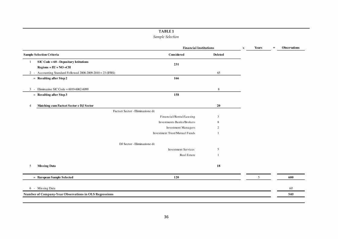
36
x Years = Observations
Considered Deleted
1 SIC Code = 60 - Depositary Istitutions
Regions = EU + NO +CH
2 - Accounting Standard Followed 2008-2009-2010 = 23 (IFRS) 65
= Resulting after Step 2 166
3 - Eliminazine SIC Code = 6019-6062-6099 8
= Resulting after Step 3 158
4 Matching cum Factset Sector e DJ Sector 20
Factset Sector - Eliminazione di:
3
8
2
1
DJ Sector - Eliminazione di:
5
1
5 Missing Data 18
= European Sample Selected 120 5 600
6 - Missing Data 60
540
TABLE 1
Sample Selection
Financial Institutions
Number of Company-Year Observations in OLS Regressions
Investment Services
Rea l Esta te
Sample Selection Criteria
231
Financia l/Renta l/Leasing
Investments Banks/Brokers
Investment Managers
Investment Trust/Mutua l Funds
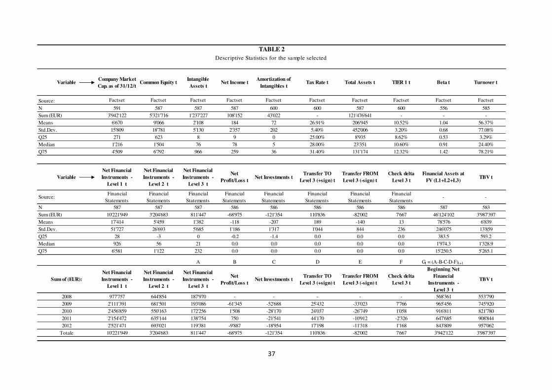
37
VariableCompany Market
Cap. as of 31/12/tCommon Equity t
Intangible
Assets tNet Income t
Amortization of
Intangibles tTax Rate t Total Assets t TIER 1 t Beta t Turnover t
Source: Factset Factset Factset Factset Factset Factset Factset Factset Factset Factset
N 591 587 587 587 600 600 587 600 556 585
Sum (EUR) 3'942'122 5'321'716 1'237'227 108'152 43'022 - 121'476'641 - - -
Means 6'670 9'066 2'108 184 72 26.91% 206'945 10.52% 1.04 56.37%
Std.Dev. 15'809 18'781 5'130 2'357 202 5.40% 452'006 3.20% 0.68 77.08%
Q25 271 623 8 9 0 25.00% 8'935 8.62% 0.53 3.29%
Median 1'216 1'504 76 78 5 28.00% 23'351 10.60% 0.91 24.40%
Q75 4'509 6'792 966 259 36 31.40% 131'174 12.32% 1.42 78.21%
Variable
Net Financial
Instruments -
Level 1 t
Net Financial
Instruments -
Level 2 t
Net Financial
Instruments -
Level 3 t
Net
Profit/Loss tNet Investments t
Transfer TO
Level 3 (+sign) t
Transfer FROM
Level 3 (-sign) t
Check delta
Level 3 t
Financial Assets at
FV (L1+L2+L3)TBV t
Source:Financial
Statements
Financial
Statements
Financial
Statements
Financial
Statements
Financial
Statements
Financial
Statements
Financial
Statements
Financial
Statements- -
N 587 587 587 586 586 586 586 586 587 583
Sum (EUR) 10'221'949 3'204'683 811'447 -68'975 -121'354 110'836 -82'002 7'667 46'124'102 3'987'397
Means 17'414 5'459 1'382 -118 -207 189 -140 13 78'576 6'839
Std.Dev. 51'727 26'693 5'685 1'186 1'317 1'044 844 236 246'075 13'859
Q25 28 -3 0 -0.2 -1.4 0.0 0.0 0.0 383.5 593.2
Median 926 56 21 0.0 0.0 0.0 0.0 0.0 1'974.3 1'328.9
Q75 6'581 1'122 232 0.0 0.0 0.0 0.0 0.0 15'250.5 5'265.1
A B C D E F Gt = (A-B-C-D-F)t+1
Sum of (EUR):
Net Financial
Instruments -
Level 1 t
Net Financial
Instruments -
Level 2 t
Net Financial
Instruments -
Level 3 t
Net
Profit/Loss tNet Investments t
Transfer TO
Level 3 (+sign) t
Transfer FROM
Level 3 (-sign) t
Check delta
Level 3 t
Beginning Net
Financial
Instruments -
Level 3 t
TBV t
2008 977'757 644'854 187'970 - - - - - 568'361 553'790
2009 2'111'391 681'501 193'086 -61'345 -52'688 25'432 -33'023 7'766 965'456 745'920
2010 2'456'859 550'163 172'256 1'508 -28'170 24'037 -26'749 1'058 916'811 821'780
2011 2'154'472 635'144 138'754 750 -21'541 44'170 -10'912 -2'326 647'685 908'844
2012 2'521'471 693'021 119'381 -9'887 -18'954 17'198 -11'318 1'168 843'809 957'062
Totale 10'221'949 3'204'683 811'447 -68'975 -121'354 110'836 -82'002 7'667 3'942'122 3'987'397
TABLE 2
Descriptive Sta tistics for the sample selected
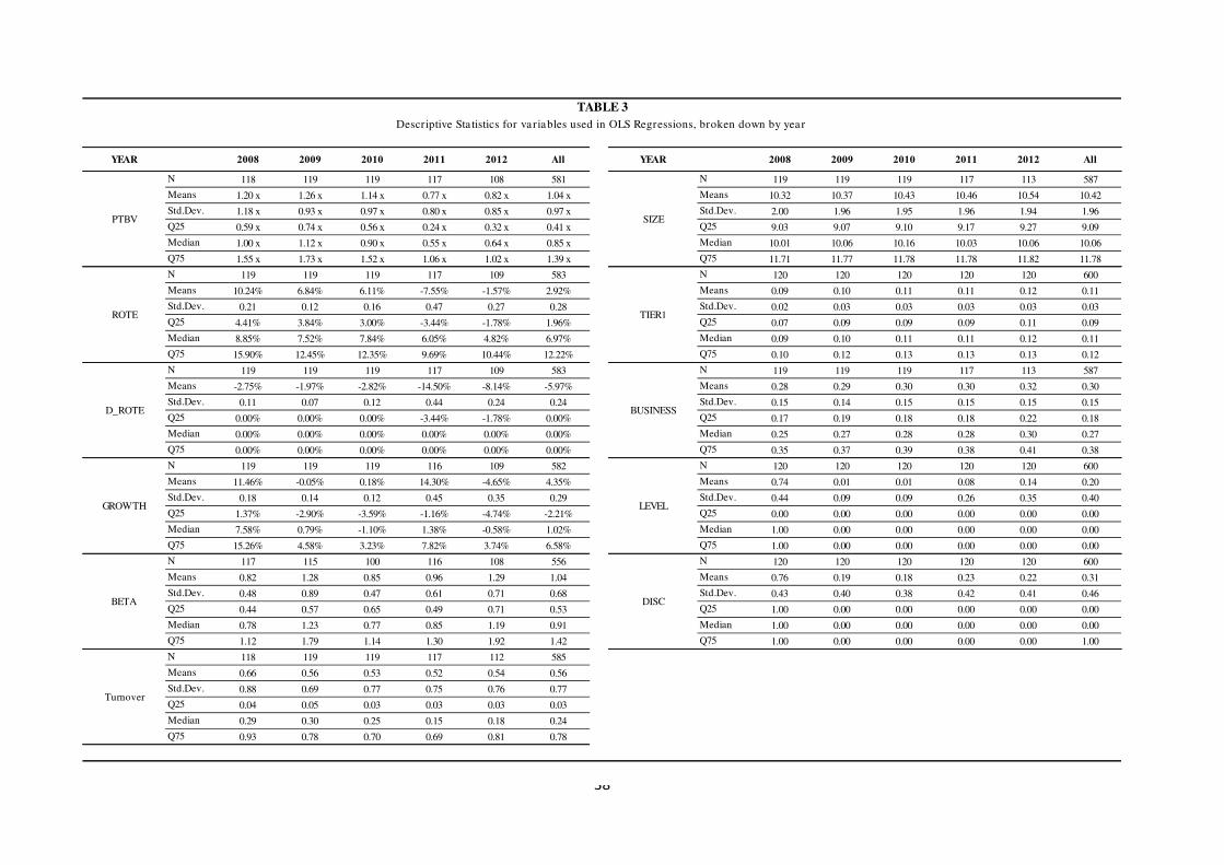
38
YEAR 2008 2009 2010 2011 2012 All YEAR 2008 2009 2010 2011 2012 All
N 118 119 119 117 108 581 N 119 119 119 117 113 587
Means 1.20 x 1.26 x 1.14 x 0.77 x 0.82 x 1.04 x Means 10.32 10.37 10.43 10.46 10.54 10.42
Std.Dev. 1.18 x 0.93 x 0.97 x 0.80 x 0.85 x 0.97 x Std.Dev. 2.00 1.96 1.95 1.96 1.94 1.96
Q25 0.59 x 0.74 x 0.56 x 0.24 x 0.32 x 0.41 x Q25 9.03 9.07 9.10 9.17 9.27 9.09
Median 1.00 x 1.12 x 0.90 x 0.55 x 0.64 x 0.85 x Median 10.01 10.06 10.16 10.03 10.06 10.06
Q75 1.55 x 1.73 x 1.52 x 1.06 x 1.02 x 1.39 x Q75 11.71 11.77 11.78 11.78 11.82 11.78
N 119 119 119 117 109 583 N 120 120 120 120 120 600
Means 10.24% 6.84% 6.11% -7.55% -1.57% 2.92% Means 0.09 0.10 0.11 0.11 0.12 0.11
Std.Dev. 0.21 0.12 0.16 0.47 0.27 0.28 Std.Dev. 0.02 0.03 0.03 0.03 0.03 0.03
Q25 4.41% 3.84% 3.00% -3.44% -1.78% 1.96% Q25 0.07 0.09 0.09 0.09 0.11 0.09
Median 8.85% 7.52% 7.84% 6.05% 4.82% 6.97% Median 0.09 0.10 0.11 0.11 0.12 0.11
Q75 15.90% 12.45% 12.35% 9.69% 10.44% 12.22% Q75 0.10 0.12 0.13 0.13 0.13 0.12
N 119 119 119 117 109 583 N 119 119 119 117 113 587
Means -2.75% -1.97% -2.82% -14.50% -8.14% -5.97% Means 0.28 0.29 0.30 0.30 0.32 0.30
Std.Dev. 0.11 0.07 0.12 0.44 0.24 0.24 Std.Dev. 0.15 0.14 0.15 0.15 0.15 0.15
Q25 0.00% 0.00% 0.00% -3.44% -1.78% 0.00% Q25 0.17 0.19 0.18 0.18 0.22 0.18
Median 0.00% 0.00% 0.00% 0.00% 0.00% 0.00% Median 0.25 0.27 0.28 0.28 0.30 0.27
Q75 0.00% 0.00% 0.00% 0.00% 0.00% 0.00% Q75 0.35 0.37 0.39 0.38 0.41 0.38
N 119 119 119 116 109 582 N 120 120 120 120 120 600
Means 11.46% -0.05% 0.18% 14.30% -4.65% 4.35% Means 0.74 0.01 0.01 0.08 0.14 0.20
Std.Dev. 0.18 0.14 0.12 0.45 0.35 0.29 Std.Dev. 0.44 0.09 0.09 0.26 0.35 0.40
Q25 1.37% -2.90% -3.59% -1.16% -4.74% -2.21% Q25 0.00 0.00 0.00 0.00 0.00 0.00
Median 7.58% 0.79% -1.10% 1.38% -0.58% 1.02% Median 1.00 0.00 0.00 0.00 0.00 0.00
Q75 15.26% 4.58% 3.23% 7.82% 3.74% 6.58% Q75 1.00 0.00 0.00 0.00 0.00 0.00
N 117 115 100 116 108 556 N 120 120 120 120 120 600
Means 0.82 1.28 0.85 0.96 1.29 1.04 Means 0.76 0.19 0.18 0.23 0.22 0.31
Std.Dev. 0.48 0.89 0.47 0.61 0.71 0.68 Std.Dev. 0.43 0.40 0.38 0.42 0.41 0.46
Q25 0.44 0.57 0.65 0.49 0.71 0.53 Q25 1.00 0.00 0.00 0.00 0.00 0.00
Median 0.78 1.23 0.77 0.85 1.19 0.91 Median 1.00 0.00 0.00 0.00 0.00 0.00
Q75 1.12 1.79 1.14 1.30 1.92 1.42 Q75 1.00 0.00 0.00 0.00 0.00 1.00
N 118 119 119 117 112 585
Means 0.66 0.56 0.53 0.52 0.54 0.56
Std.Dev. 0.88 0.69 0.77 0.75 0.76 0.77
Q25 0.04 0.05 0.03 0.03 0.03 0.03
Median 0.29 0.30 0.25 0.15 0.18 0.24
Q75 0.93 0.78 0.70 0.69 0.81 0.78
TABLE 3
Descriptive Sta tistics for variables used in OLS Regressions, broken down by year
SIZE
TIER1
BUSINESS
LEVEL
DISC
PTBV
ROTE
D_ROTE
GROWTH
BETA
Turnover
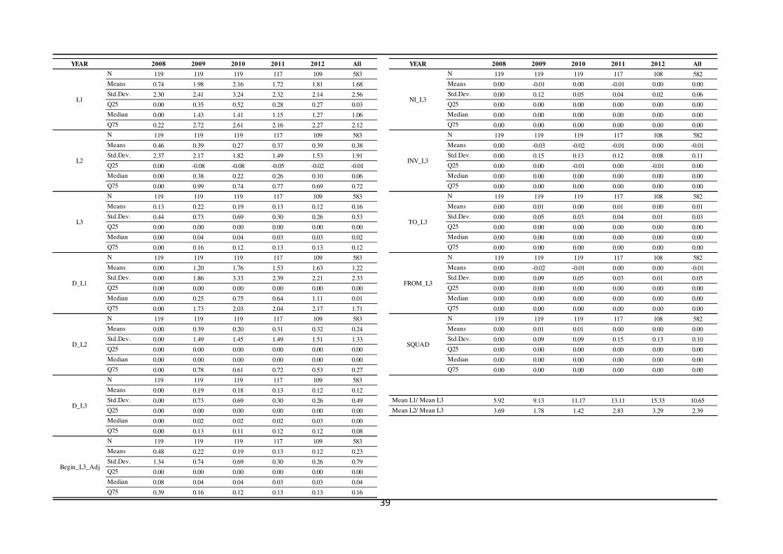
39
YEAR 2008 2009 2010 2011 2012 All YEAR 2008 2009 2010 2011 2012 All
N 119 119 119 117 109 583 N 119 119 119 117 108 582
Means 0.74 1.98 2.16 1.72 1.81 1.68 Means 0.00 -0.01 0.00 -0.01 0.00 0.00
Std.Dev. 2.30 2.41 3.24 2.32 2.14 2.56 Std.Dev. 0.00 0.12 0.05 0.04 0.02 0.06
Q25 0.00 0.35 0.52 0.28 0.27 0.03 Q25 0.00 0.00 0.00 0.00 0.00 0.00
Median 0.00 1.43 1.41 1.15 1.27 1.06 Median 0.00 0.00 0.00 0.00 0.00 0.00
Q75 0.22 2.72 2.61 2.16 2.27 2.12 Q75 0.00 0.00 0.00 0.00 0.00 0.00
N 119 119 119 117 109 583 N 119 119 119 117 108 582
Means 0.46 0.39 0.27 0.37 0.39 0.38 Means 0.00 -0.03 -0.02 -0.01 0.00 -0.01
Std.Dev. 2.37 2.17 1.82 1.49 1.53 1.91 Std.Dev. 0.00 0.15 0.13 0.12 0.08 0.11
Q25 0.00 -0.08 -0.08 -0.05 -0.02 -0.01 Q25 0.00 0.00 -0.01 0.00 -0.01 0.00
Median 0.00 0.38 0.22 0.26 0.10 0.06 Median 0.00 0.00 0.00 0.00 0.00 0.00
Q75 0.00 0.99 0.74 0.77 0.69 0.72 Q75 0.00 0.00 0.00 0.00 0.00 0.00
N 119 119 119 117 109 583 N 119 119 119 117 108 582
Means 0.13 0.22 0.19 0.13 0.12 0.16 Means 0.00 0.01 0.00 0.01 0.00 0.01
Std.Dev. 0.44 0.73 0.69 0.30 0.26 0.53 Std.Dev. 0.00 0.05 0.03 0.04 0.01 0.03
Q25 0.00 0.00 0.00 0.00 0.00 0.00 Q25 0.00 0.00 0.00 0.00 0.00 0.00
Median 0.00 0.04 0.04 0.03 0.03 0.02 Median 0.00 0.00 0.00 0.00 0.00 0.00
Q75 0.00 0.16 0.12 0.13 0.13 0.12 Q75 0.00 0.00 0.00 0.00 0.00 0.00
N 119 119 119 117 109 583 N 119 119 119 117 108 582
Means 0.00 1.20 1.76 1.53 1.63 1.22 Means 0.00 -0.02 -0.01 0.00 0.00 -0.01
Std.Dev. 0.00 1.86 3.33 2.39 2.21 2.33 Std.Dev. 0.00 0.09 0.05 0.03 0.01 0.05
Q25 0.00 0.00 0.00 0.00 0.00 0.00 Q25 0.00 0.00 0.00 0.00 0.00 0.00
Median 0.00 0.25 0.75 0.64 1.11 0.01 Median 0.00 0.00 0.00 0.00 0.00 0.00
Q75 0.00 1.73 2.03 2.04 2.17 1.71 Q75 0.00 0.00 0.00 0.00 0.00 0.00
N 119 119 119 117 109 583 N 119 119 119 117 108 582
Means 0.00 0.39 0.20 0.31 0.32 0.24 Means 0.00 0.01 0.01 0.00 0.00 0.00
Std.Dev. 0.00 1.49 1.45 1.49 1.51 1.33 Std.Dev. 0.00 0.09 0.09 0.15 0.13 0.10
Q25 0.00 0.00 0.00 0.00 0.00 0.00 Q25 0.00 0.00 0.00 0.00 0.00 0.00
Median 0.00 0.00 0.00 0.00 0.00 0.00 Median 0.00 0.00 0.00 0.00 0.00 0.00
Q75 0.00 0.78 0.61 0.72 0.53 0.27 Q75 0.00 0.00 0.00 0.00 0.00 0.00
N 119 119 119 117 109 583
Means 0.00 0.19 0.18 0.13 0.12 0.12
Std.Dev. 0.00 0.73 0.69 0.30 0.26 0.49 Mean L1/ Mean L3 5.92 9.13 11.17 13.11 15.33 10.65
Q25 0.00 0.00 0.00 0.00 0.00 0.00 Mean L2/ Mean L3 3.69 1.78 1.42 2.83 3.29 2.39
Median 0.00 0.02 0.02 0.02 0.03 0.00
Q75 0.00 0.13 0.11 0.12 0.12 0.08
N 119 119 119 117 109 583
Means 0.48 0.22 0.19 0.13 0.12 0.23
Std.Dev. 1.34 0.74 0.69 0.30 0.26 0.79
Q25 0.00 0.00 0.00 0.00 0.00 0.00
Median 0.08 0.04 0.04 0.03 0.03 0.04
Q75 0.39 0.16 0.12 0.13 0.13 0.16
L3
D_L1
D_L2
D_L3
Begin_L3_Adj
NI_L3
INV_L3
TO_L3
FROM_L3
SQUAD
L2
L1
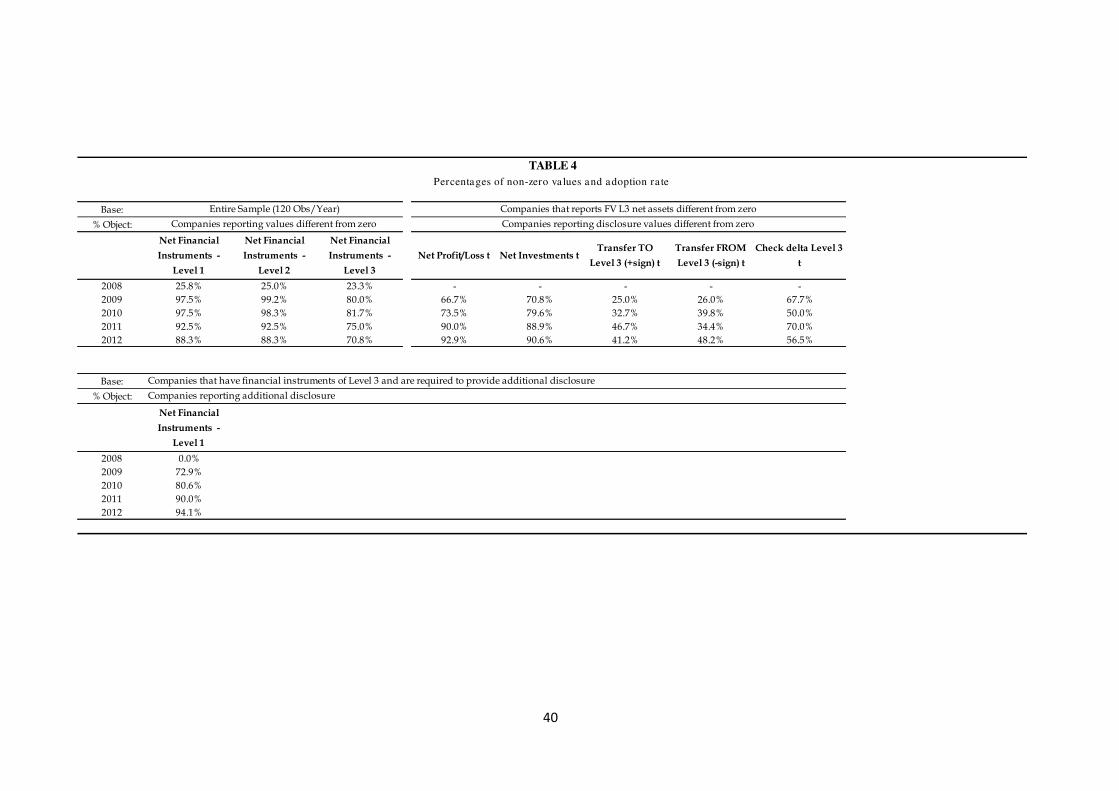
40
Base:
% Object:
Net Financial
Instruments -
Level 1
Net Financial
Instruments -
Level 2
Net Financial
Instruments -
Level 3
Net Profit/Loss t Net Investments tTransfer TO
Level 3 (+sign) t
Transfer FROM
Level 3 (-sign) t
Check delta Level 3
t
2008 25.8% 25.0% 23.3% - - - - -
2009 97.5% 99.2% 80.0% 66.7% 70.8% 25.0% 26.0% 67.7%
2010 97.5% 98.3% 81.7% 73.5% 79.6% 32.7% 39.8% 50.0%
2011 92.5% 92.5% 75.0% 90.0% 88.9% 46.7% 34.4% 70.0%
2012 88.3% 88.3% 70.8% 92.9% 90.6% 41.2% 48.2% 56.5%
Base:
% Object:
Net Financial
Instruments -
Level 1
2008 0.0%
2009 72.9%
2010 80.6%
2011 90.0%
2012 94.1%
Companies that have financial instruments of Level 3 and are required to provide additional disclosure
Companies reporting additional disclosure
TABLE 4
Percentages of non-zero va lues and adoption ra te
Companies reporting values different from zero Companies reporting disclosure values different from zero
Entire Sample (120 Obs/Year) Companies that reports FV L3 net assets different from zero
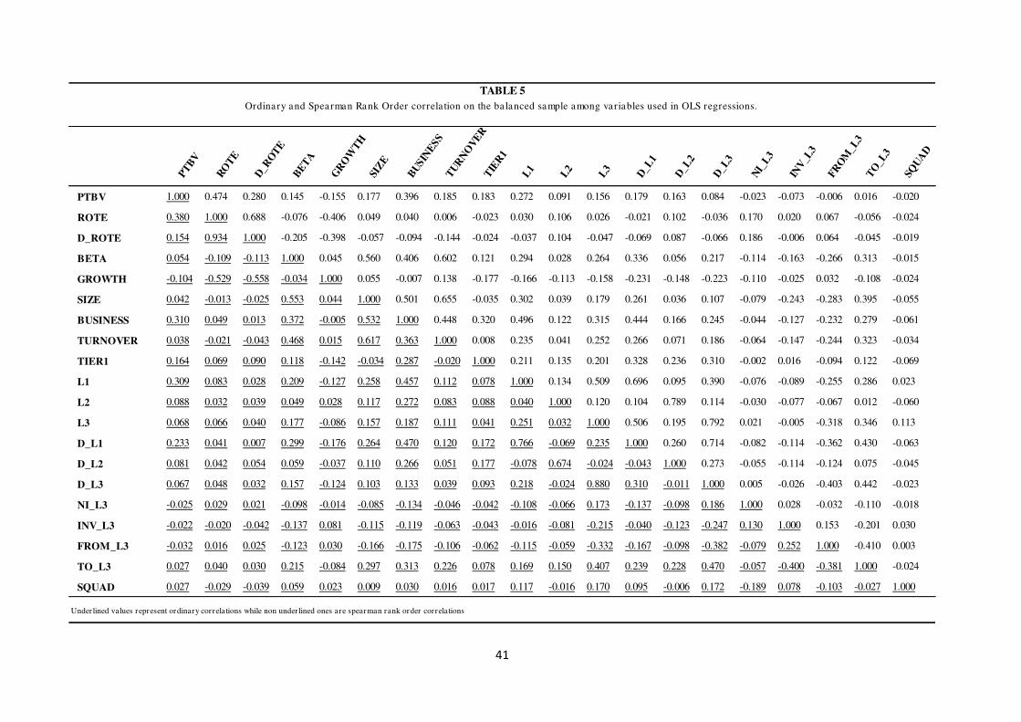
41
TABLE 5
Ordinary and Spearman Rank Order correla tion on the ba lanced sample among variables used in OLS regressions.
PT
BV
RO
TE
D_R
OT
E
BE
TA
GR
OW
TH
SIZ
E
BU
SIN
ESS
TU
RN
OV
ER
TIE
R1
L1
L2
L3
D_L
1
D_L
2
D_L
3
NI_
L3
IN
V_L
3
FR
OM
_L3
TO
_L3
SQ
UA
D
PTBV 1.000 0.474 0.280 0.145 -0.155 0.177 0.396 0.185 0.183 0.272 0.091 0.156 0.179 0.163 0.084 -0.023 -0.073 -0.006 0.016 -0.020
ROTE 0.380 1.000 0.688 -0.076 -0.406 0.049 0.040 0.006 -0.023 0.030 0.106 0.026 -0.021 0.102 -0.036 0.170 0.020 0.067 -0.056 -0.024
D_ROTE 0.154 0.934 1.000 -0.205 -0.398 -0.057 -0.094 -0.144 -0.024 -0.037 0.104 -0.047 -0.069 0.087 -0.066 0.186 -0.006 0.064 -0.045 -0.019
BETA 0.054 -0.109 -0.113 1.000 0.045 0.560 0.406 0.602 0.121 0.294 0.028 0.264 0.336 0.056 0.217 -0.114 -0.163 -0.266 0.313 -0.015
GROWTH -0.104 -0.529 -0.558 -0.034 1.000 0.055 -0.007 0.138 -0.177 -0.166 -0.113 -0.158 -0.231 -0.148 -0.223 -0.110 -0.025 0.032 -0.108 -0.024
SIZE 0.042 -0.013 -0.025 0.553 0.044 1.000 0.501 0.655 -0.035 0.302 0.039 0.179 0.261 0.036 0.107 -0.079 -0.243 -0.283 0.395 -0.055
BUSINESS 0.310 0.049 0.013 0.372 -0.005 0.532 1.000 0.448 0.320 0.496 0.122 0.315 0.444 0.166 0.245 -0.044 -0.127 -0.232 0.279 -0.061
TURNOVER 0.038 -0.021 -0.043 0.468 0.015 0.617 0.363 1.000 0.008 0.235 0.041 0.252 0.266 0.071 0.186 -0.064 -0.147 -0.244 0.323 -0.034
TIER1 0.164 0.069 0.090 0.118 -0.142 -0.034 0.287 -0.020 1.000 0.211 0.135 0.201 0.328 0.236 0.310 -0.002 0.016 -0.094 0.122 -0.069
L1 0.309 0.083 0.028 0.209 -0.127 0.258 0.457 0.112 0.078 1.000 0.134 0.509 0.696 0.095 0.390 -0.076 -0.089 -0.255 0.286 0.023
L2 0.088 0.032 0.039 0.049 0.028 0.117 0.272 0.083 0.088 0.040 1.000 0.120 0.104 0.789 0.114 -0.030 -0.077 -0.067 0.012 -0.060
L3 0.068 0.066 0.040 0.177 -0.086 0.157 0.187 0.111 0.041 0.251 0.032 1.000 0.506 0.195 0.792 0.021 -0.005 -0.318 0.346 0.113
D_L1 0.233 0.041 0.007 0.299 -0.176 0.264 0.470 0.120 0.172 0.766 -0.069 0.235 1.000 0.260 0.714 -0.082 -0.114 -0.362 0.430 -0.063
D_L2 0.081 0.042 0.054 0.059 -0.037 0.110 0.266 0.051 0.177 -0.078 0.674 -0.024 -0.043 1.000 0.273 -0.055 -0.114 -0.124 0.075 -0.045
D_L3 0.067 0.048 0.032 0.157 -0.124 0.103 0.133 0.039 0.093 0.218 -0.024 0.880 0.310 -0.011 1.000 0.005 -0.026 -0.403 0.442 -0.023
NI_L3 -0.025 0.029 0.021 -0.098 -0.014 -0.085 -0.134 -0.046 -0.042 -0.108 -0.066 0.173 -0.137 -0.098 0.186 1.000 0.028 -0.032 -0.110 -0.018
INV_L3 -0.022 -0.020 -0.042 -0.137 0.081 -0.115 -0.119 -0.063 -0.043 -0.016 -0.081 -0.215 -0.040 -0.123 -0.247 0.130 1.000 0.153 -0.201 0.030
FROM_L3 -0.032 0.016 0.025 -0.123 0.030 -0.166 -0.175 -0.106 -0.062 -0.115 -0.059 -0.332 -0.167 -0.098 -0.382 -0.079 0.252 1.000 -0.410 0.003
TO_L3 0.027 0.040 0.030 0.215 -0.084 0.297 0.313 0.226 0.078 0.169 0.150 0.407 0.239 0.228 0.470 -0.057 -0.400 -0.381 1.000 -0.024
SQUAD 0.027 -0.029 -0.039 0.059 0.023 0.009 0.030 0.016 0.017 0.117 -0.016 0.170 0.095 -0.006 0.172 -0.189 0.078 -0.103 -0.027 1.000
Underlined values represent ordinary correlations while non underlined ones are spearman rank order correlations
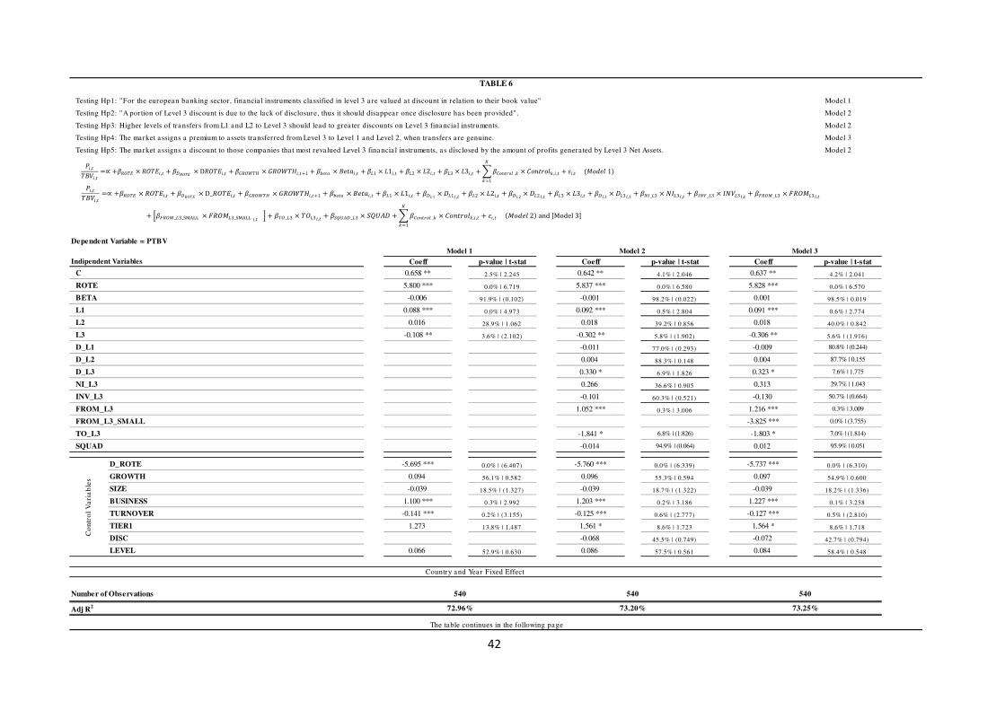
42
Dependent Variable = PTBV
Coeff p-value | t-stat Coeff p-value | t-stat Coeff p-value | t-stat
C 0.658 ** 2.5% | 2.245 0.642 ** 4.1% | 2.046 0.637 ** 4.2% | 2.041
ROTE 5.800 *** 0.0% | 6.719 5.837 *** 0.0% | 6.580 5.828 *** 0.0% | 6.570
BETA -0.006 91.9% | (0.102) -0.001 98.2% | (0.022) 0.001 98.5% | 0.019
L1 0.088 *** 0.0% | 4.973 0.092 *** 0.5% | 2.804 0.091 *** 0.6% | 2.774
L2 0.016 28.9% | 1.062 0.018 39.2% | 0.856 0.018 40.0% | 0.842
L3 -0.108 ** 3.6% | (2.102) -0.302 ** 5.8% | (1.902) -0.306 ** 5.6% | (1.916)
D_L1 -0.011 77.0% | (0.293) -0.009 80.8% | (0.244)
D_L2 0.004 88.3% | 0.148 0.004 87.7% | 0.155
D_L3 0.330 * 6.9% | 1.826 0.323 * 7.6% | 1.775
NI_L3 0.266 36.6% | 0.905 0.313 29.7% | 1.043
INV_L3 -0.101 60.3% | (0.521) -0.130 50.7% | (0.664)
FROM_L3 1.052 *** 0.3% | 3.006 1.216 *** 0.3% | 3.009
FROM_L3_SMALL -3.825 *** 0.0% | (3.755)
TO_L3 -1.841 * 6.8% | (1.826) -1.803 * 7.0% | (1.814)
SQUAD -0.014 94.9% | (0.064) 0.012 95.9% | 0.051
D_ROTE -5.695 *** 0.0% | (6.407) -5.760 *** 0.0% | (6.339) -5.737 *** 0.0% | (6.310)
GROWTH 0.094 56.1% | 0.582 0.096 55.3% | 0.594 0.097 54.9% | 0.600
SIZE -0.039 18.5% | (1.327) -0.039 18.7% | (1.322) -0.039 18.2% | (1.336)
BUSINESS 1.100 *** 0.3% | 2.992 1.203 *** 0.2% | 3.186 1.227 *** 0.1% | 3.258
TURNOVER -0.141 *** 0.2% | (3.155) -0.125 *** 0.6% | (2.777) -0.127 *** 0.5% | (2.810)
TIER1 1.273 13.8% | 1.487 1.561 * 8.6% | 1.723 1.564 * 8.6% | 1.718
DISC -0.068 45.5% | (0.749) -0.072 42.7% | (0.794)
LEVEL 0.066 52.9% | 0.630 0.086 57.5% | 0.561 0.084 58.4% | 0.548
Number of Observations
Adj R2
540 540 540
72.96% 73.20% 73.25%
The table continues in the following page
Model 1 Model 2 Model 3
Indipendent Variables
Co
ntr
ol
Va
ria
ble
s
Country and Year Fixed Effect
Testing Hp3: Higher levels of transfers from L1 and L2 to Level 3 should lead to grea ter discounts on Level 3 financia l instruments. Model 2
Testing Hp4: The market assigns a premium to assets transferred from Level 3 to Level 1 and Level 2, when transfers a re genuine. Model 3
Testing Hp5: The market assigns a discount to those companies tha t most reva lued Level 3 financia l instruments, as disclosed by the amount of profits genera ted by Level 3 Net Assets. Model 2
TABLE 6
Testing Hp1: "For the european banking sector, financia l instruments classified in level 3 a re va lued a t discount in rela tion to their book va lue" Model 1
Testing Hp2: "A portion of Level 3 discount is due to the lack of disclosure, thus it should disappear once disclosure has been provided". Model 2
,
,
=∝ + × , + × D , + × , +1 + × , + 1 × 1 , + 2 × 2 , + 3 × 3 , + , × , ,
=1
+ , ( 1)
,
,
=∝ + × , + × D_ , + × , +1 + × , + 1 × 1 , +1
× 1 ,+ 2 × 2 , +
2× 2 ,
+ 3 × 3 , +3
× 3 ,+ _ 3 × 3 ,
+ _ 3 × 3 ,+ _ 3 × 3 ,
+ _ 3_SMALL × 3_SMALL , + _ 3 × 3 ,
+ _ 3 × + , × , ,
=1
+ , 2 and Model 3
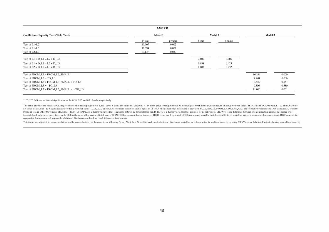
43
Coefficients Equality Test (Wald Test)
F-stat p-value F-stat p-value
Test of L1=L2 10.007 0.002
Test of L1=L3 12.394 0.001
Test of L2=L3 5.409 0.020
Test of L1 + D_L1 = L2 + D_L2 7.800 0.005
Test of L1 + D_L1 = L3 + D_L3 0.638 0.425
Test of L2 + D_L2 = L3 + D_L3 0.007 0.932
Test of FROM_L3 = FROM_L3_SMALL 16.236 0.000
Test of FROM_L3 = TO_L3 7.740 0.006
Test of FROM_L3 + FROM_L3_SMALL = TO_L3 0.345 0.557
Test of FROM_L3 = - TO_L3 0.306 0.580
Test of FROM_L3 + FROM_L3_SMALL = - TO_L3 11.060 0.001
This table provides the results of OLS regression used in testing hypothesis 1, tha t Level 3 assets a re va lued a t discount. PTBV is the price to tangible book va lue multiple, ROTE is the adjusted return on tangible book va lue, BETA is bank's CAPM beta , L1, L2 and L3 a re the
net amounts of Level 1 to 3 assets sca led over tangible book va lue, D_L1,D_L2 and D_L3 a re dummy variables tha t is equa l to L1 to L3 when additiona l disclosure is provided, NI_L3, INV_L3, FROM_L3, TO_L3 SQUAD are respectively Net income, Net Investments, Transfer
from and to and Other Movements of Level 3, FROM_L3_SMALL is a dummy variable tha t is equa l to FROM_L3 for small transfer. D_ROTE is a dummy variables tha t controls for nega tive rote, GROWTH is the difference between two consecutive net incomes sca led over
tangible book va lue as a proxy for growth, SIZE is the na tura l logharitm of tota l a ssets, TURNOVER is common shares' turnover, TIER1 is the tier 1 ra tio and LEVEL is a dummy variable tha t detects if L1 to L3 variables a re zero because of disclosure, while DISC controls for
companies tha t do not need to provide additiona l disclosure, not holding Level 3 financia l instruments.
T-sta tistics a re adjusted for autocorrela tion and heteroscedasticity in the error term, following Newey-West. Fa ir Va lue Hiera rchy and additiona l disclosure va riables have been tested for multicollinea rity by using VIF (Variance Infla tion Factor), showing no multicollinea rity
CONT'D
Model 1 Model 2 Model 3
*, **, *** Indica te sta tistica l significance a t the 0.10, 0.05 and 0.01 levels, respectively
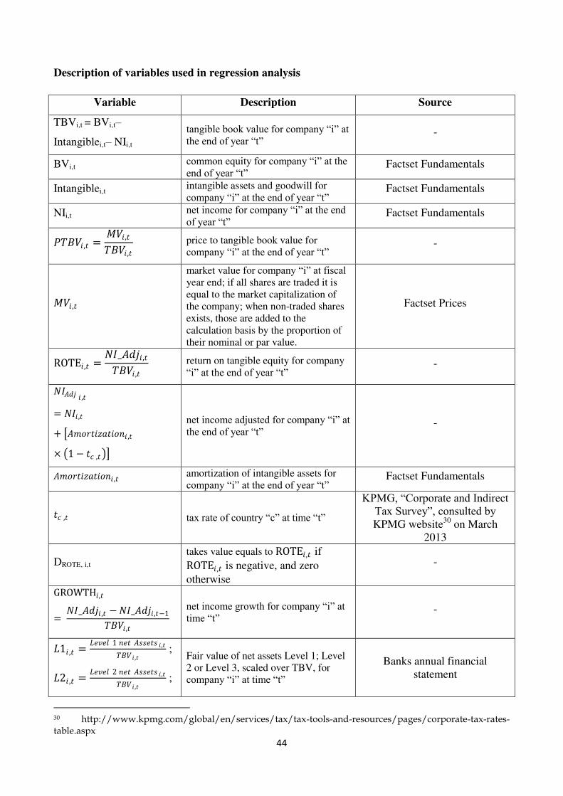
44
Description of variables used in regression analysis
Variable Description Source
TBVi,t = BVi,t–
Intangiblei,t– NIi,t
tangible book value for company ―i‖ at the end of year ―t‖
-
BVi,t common equity for company ―i‖ at the end of year ―t‖
Factset Fundamentals
Intangiblei,t intangible assets and goodwill for
company ―i‖ at the end of year ―t‖ Factset Fundamentals
NIi,t net income for company ―i‖ at the end of year ―t‖
Factset Fundamentals
, =,
,
price to tangible book value for
company ―i‖ at the end of year ―t‖ -
,
market value for company ―i‖ at fiscal year end; if all shares are traded it is
equal to the market capitalization of
the company; when non-traded shares
exists, those are added to the
calculation basis by the proportion of
their nominal or par value.
Factset Prices
ROTE , =_ ,
,
return on tangible equity for company
―i‖ at the end of year ―t‖ -
,
= ,
+ � ,
× 1 − , net income adjusted for company ―i‖ at the end of year ―t‖
-
� , amortization of intangible assets for
company ―i‖ at the end of year ―t‖ Factset Fundamentals
, tax rate of country ―c‖ at time ―t‖
KPMG, ―Corporate and Indirect Tax Survey‖, consulted by KPMG website
30 on March
2013
DROTE, i,t takes value equals to ROTE , if
ROTE , is negative, and zero
otherwise
-
GROWTH ,
= _ , − _ , −1
,
net income growth for company ―i‖ at time ―t‖
-
1 , = 1 ,
, ;
2 , = 2 ,
, ;
Fair value of net assets Level 1; Level
2 or Level 3, scaled over TBV, for
company ―i‖ at time ―t‖
Banks annual financial
statement
30 http://www.kpmg.com/global/en/services/tax/tax-tools-and-resources/pages/corporate-tax-rates-table.aspx
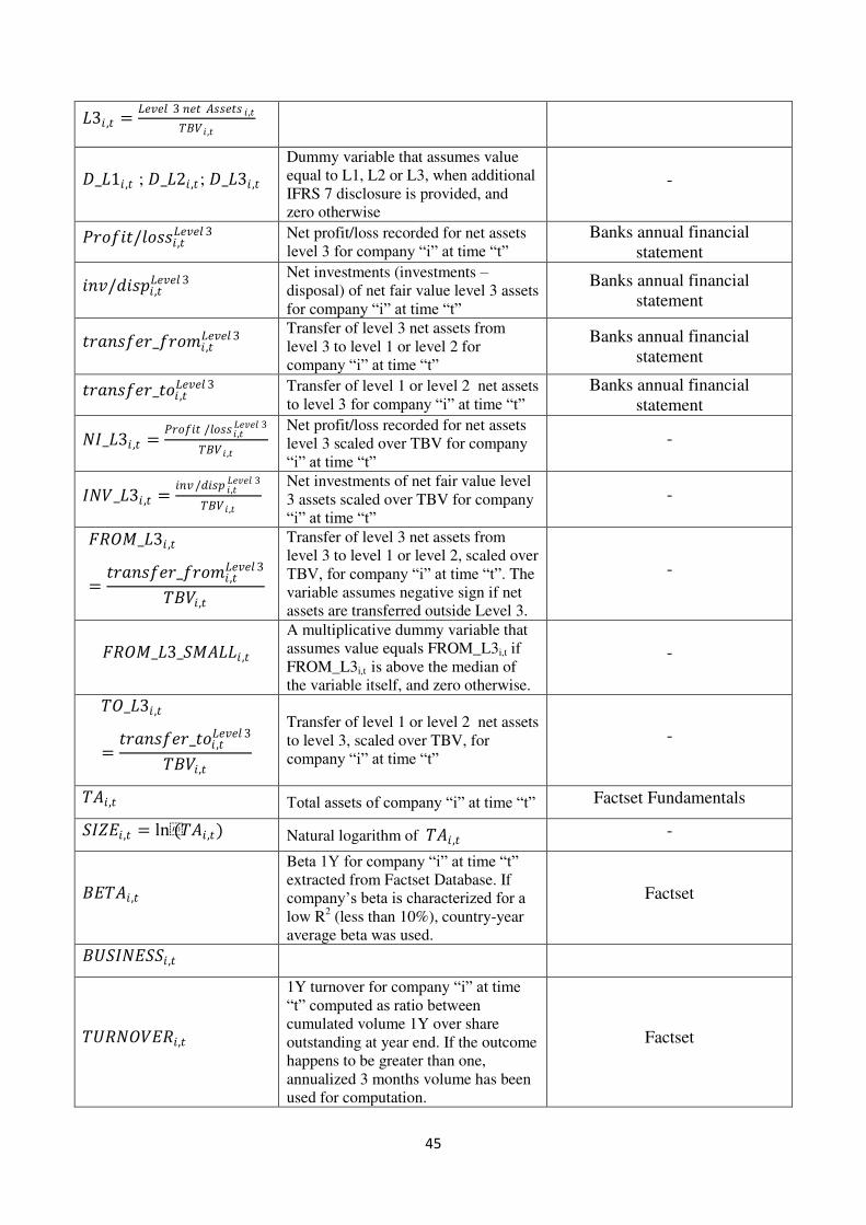
45
3 , = 3 ,
,
_ 1 , ; _ 2 , ; _ 3 ,
Dummy variable that assumes value
equal to L1, L2 or L3, when additional
IFRS 7 disclosure is provided, and
zero otherwise
-
/ ,3 Net profit/loss recorded for net assets
level 3 for company ―i‖ at time ―t‖
Banks annual financial
statement
/ ,3
Net investments (investments –
disposal) of net fair value level 3 assets
for company ―i‖ at time ―t‖
Banks annual financial
statement
_ ,3
Transfer of level 3 net assets from
level 3 to level 1 or level 2 for
company ―i‖ at time ―t‖
Banks annual financial
statement
_ ,3 Transfer of level 1 or level 2 net assets
to level 3 for company ―i‖ at time ―t‖
Banks annual financial
statement
_ 3 , =/ ,
3
,
Net profit/loss recorded for net assets
level 3 scaled over TBV for company
―i‖ at time ―t‖
-
_ 3 , =/ ,
3
,
Net investments of net fair value level
3 assets scaled over TBV for company
―i‖ at time ―t‖
-
_ 3 ,
=_ ,
3
,
Transfer of level 3 net assets from
level 3 to level 1 or level 2, scaled over
TBV, for company ―i‖ at time ―t‖. The
variable assumes negative sign if net
assets are transferred outside Level 3.
-
_ 3_ ,
A multiplicative dummy variable that
assumes value equals FROM_L3i,t if
FROM_L3i,t is above the median of
the variable itself, and zero otherwise.
-
_ 3 ,
=_ ,
3
,
Transfer of level 1 or level 2 net assets
to level 3, scaled over TBV, for
company ―i‖ at time ―t‖
-
, Total assets of company ―i‖ at time ―t‖ Factset Fundamentals
, = ln( , ) Natural logarithm of , -
,
Beta 1Y for company ―i‖ at time ―t‖ extracted from Factset Database. If
company’s beta is characterized for a low R
2 (less than 10%), country-year
average beta was used.
Factset
,
,
1Y turnover for company ―i‖ at time ―t‖ computed as ratio between cumulated volume 1Y over share
outstanding at year end. If the outcome
happens to be greater than one,
annualized 3 months volume has been
used for computation.
Factset
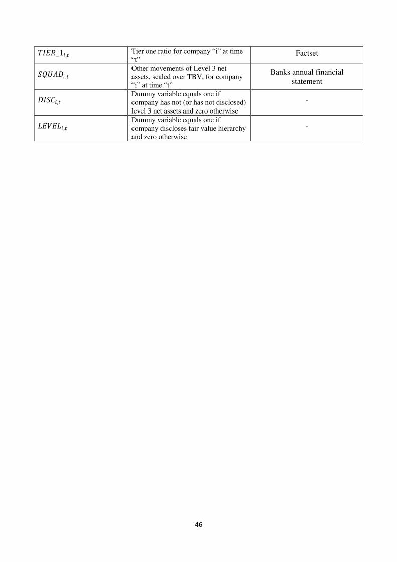
46
_1 , Tier one ratio for company ―i‖ at time ―t‖
Factset
, Other movements of Level 3 net
assets, scaled over TBV, for company
―i‖ at time ―t‖
Banks annual financial
statement
, Dummy variable equals one if
company has not (or has not disclosed)
level 3 net assets and zero otherwise
-
, Dummy variable equals one if
company discloses fair value hierarchy
and zero otherwise
-


![Improving Maslow’s Hierarchy of Needs: New Approach to ...€¦ · Maslow’s Hierarchy of Needs – 1970 Expression [41] Level in Hierarchy Maslow Need Description 7 Aesthetic](https://img.pdfslide.us/doc/110x75/5f4b71e1c352b64dde2f3478/improving-maslowas-hierarchy-of-needs-new-approach-to-maslowas-hierarchy.jpg)