Embed Size (px)
Citation preview

Reports of the Department of Mathematical Information TechnologySeries B. Scientific ComputingNo. B 1/2015
An analytical–numerical study of dynamicstability of an axially moving elastic web
Nikolay Banichuk Alexander Barsuk
Pekka Neittaanmaki Juha Jeronen
Tero Tuovinen
University of JyvaskylaDepartment of Mathematical Information Technology
P.O. Box 35 (Agora)FI–40014 University of Jyvaskyla
FINLANDfax +358 14 260 2771
http://www.mit.jyu.fi/

Copyright c© 2015Nikolay Banichuk and Alexander Barsuk and Pekka Neittaanmaki
and Juha Jeronen and Tero Tuovinenand University of Jyvaskyla
ISBN 978-951-39-6070-4
978-951-39-6079-7 (PDF)
ISSN 1456-436X

An analytical–numerical study of dynamicstability of an axially moving elastic web∗
Nikolay Banichuk Alexander Barsuk Pekka NeittaanmakiJuha Jeronen Tero Tuovinen
Abstract
This paper is devoted to a dynamic stability analysis of an axially movingelastic web, modelled as a panel (a plate undergoing cylindrical deformation).The results are directly applicable also to the travelling beam. In accordancewith the dynamic approach of stability analysis, the problem of harmonic vi-brations is investigated via the study of the dependences of the system’s nat-ural frequencies on the problem parameters. Analytical implicit expressionsfor the solution curves, with respect to problem parameters, are derived forranges of the parameter space where the natural frequencies are real-valued,corresponding to stable vibrations. Both axially tensioned and non-tensionedtravelling panels are considered. The special cases of the non-tensioned trav-elling panel, and the tensioned stationary (non-travelling) panel are also dis-cussed, and special-case solutions given. Numerical evaluation of the obtainedgeneral analytical results is discussed. Numerical examples are given for panelssubjected to two different tension levels, and for the non-tensioned panel. Theresults allow the development of very efficient, lightweight solvers for deter-mining the natural frequencies of travelling panels and beams. The results canalso be used to help locate the bifurcation points of the solution curves, corre-sponding to points where mechanical stability is lost.
1 Introduction
The study of the dynamic behaviour of axially moving elastic systems has attractedthe attention of researchers for a long time, beginning with Skutch [1897]. Stud-ies written in the English language began to appear half a century later, startingwith those by Sack [1954], Archibald and Emslie [1958], Miranker [1960]. Otherclassic studies of moving elastic systems include those by Mote [1968a,b], Thurmanand Mote [1969], Mote [1972], Simpson [1973], Mote [1975], Mujumdar and Douglas
∗This research was supported by RFBR (grant 14-08-00016-a), RAS Program 12, Program of Sup-port of Leading Scientific Schools (grant 2954.2014.1), and the Finnish Cultural Foundation.
1

[1976], Pramila [1986, 1987], Wickert and Mote [1989]. Recent studies include Parker[1998, 1999], Kong and Parker [2004], Wang et al. [2005] and Banichuk et al. [2014b].
Of particular interest for this class of problems is the analysis of stability. A com-mon method of investigating the stability of elastic systems is the dynamic methoddue to Bolotin [1963]. In accordance with this method, we solve the problem of har-monic vibrations of the investigated system, followed by analysis of the dependenceof the behaviour of the natural frequencies as a function of the system parameters.
In the dynamic method, the appearance of complex-valued frequencies is inter-preted as a loss of stability in a dynamic form (also known as flutter), correspondingto the loss of Lyapunov stability. A convergence of the frequencies to zero corre-sponds to a loss of stability in a static form (divergence), and meets the criteria ofEuler buckling.
In this paper, we will derive analytical implicit expressions for the solution curves,with respect to problem parameters, for ranges of the parameter space where thenatural frequencies are real-valued, corresponding to stable vibrations. Both axiallytensioned and non-tensioned travelling panels will be considered. The special casesof the non-tensioned travelling panel, and the tensioned stationary (non-travelling)panel will also be discussed, and special-case solutions given.
In the following sections, we will first set up the problem, after which we willdiscuss the solution strategy. Then the analytical part of the problem will be solved,and special cases and numerical considerations discussed. Finally, numerical exam-ples will be given.
The results allow the development of very efficient, lightweight solvers for de-termining the natural frequencies of travelling panels and beams. However, moreimportantly from a fundamental research perspective, when combined with bifur-cation theory, the obtained analytical formulas can also be used to help locate thebifurcation points of the solution curves in the travelling panel (beam) model, cor-responding to points where mechanical stability is lost. By a variational argument,it is easily shown that at bifurcation points, the tangent of the local branch of thesolution curve in the (V0, ω) plane becomes vertical (Banichuk et al., 2014a). Theobtained analytical formulas can be used as tools to help find such points.
2 Basic relations
Consider an axially travelling rectangular plate undergoing cylindrical deformation,as shown in Figure 1. The equation of small transverse vibrations is
m∂2w
∂t2+ 2mV0
∂2w
∂x∂t+ (mV 2
0 − T0)∂2w
∂x2+D
∂4w
∂x4= 0 , 0 < x < ` , (1)
where m = ρS is the mass of the panel per unit area, ρ is the density of the material,S the area of the cross section, and V0 is a constant axial transport velocity. Theaxial tension T0 has the dimension of force per unit length; for a panel, it can beexpressed as T0 = hσx, where h is the thickness of the panel and σx is the axial stress.
2

(a) (b)
Figure 1: Axially travelling panel, i.e. plate undergoing cylindrical deformation.The pairs of rollers denote simple supports, and the finite thickness depicts the pres-ence of bending resistance. (a): Problem setup. (b): Projection to the xz plane.
The quantity D is the bending rigidity (also known as flexural rigidity or cylindricalrigidity), and for an isotropic elastic material it follows the relation (Timoshenkoand Woinowsky-Krieger, 1959)
D =Eh3
12(1− ν2), (2)
where E is the Young’s modulus of the material and ν its Poisson ratio. The sym-bol ` denotes the length of the free span between mechanical supports. The trans-verse (out-of-plane) displacement of the panel, as it appears in laboratory coordi-nates (also known as an Eulerian or spatial formulation) is described by the functionw ≡ w(x, t).
Equation (1) is of the fourth order in x, so four boundary conditions are neededin total. In what follows, the simply supported (also known as pinned or hinged)boundary conditions of the Kirchhoff plate (or Euler–Bernoulli beam) are used, i.e.
w(0, t) = w(`, t) = 0 , (3)
D∂2w
∂x2(0, t) = D
∂2w
∂x2(`, t) = 0 . (4)
The boundary conditions (3)–(4) arise by requiring that the transverse displace-ments and the bending moments at the boundary points x = 0 and x = ` are zero.
Harmonic vibrations of the moving panel are represented as
w(x, t) = eiωtu(x) , (5)
where u(x) is the amplitude function and ω is the frequency of vibration. It will beconvenient to work in dimensionless variables. Let us define
x = `x ,ρSω2`4
D= ω2 ,
ρS`2
DV 20 = V 2
0 ,
ρS`2
DC2 = C2 , C =
√T
ρS.
(6)
3
Note that from the chain rule, ∂(·)/∂x → (1/`)∂(·)/∂x. In the following, the tildewill be omitted.
We formulate the boundary-value problem for the amplitude function u(x) as
d4u
dx4+ (V 2
0 − C2)d2u
dx2+ 2iωV0
du
dx− ω2u = 0 , 0 < x < 1 , (7)
u(0) = u(1) = 0 ,
(d2u
dx2
)x=0
=
(d2u
dx2
)x=1
= 0 . (8)
3 Solution strategy
The amplitude function is found as a fundamental solution,
u(x) = eiγx , 0 < x < 1 , (9)
of the ordinary differential equation (7) with boundary conditions (8). Here γ is thewave number. Consequently, the displacement function will be described by theexpression
w = w(x, t) = eiωtu(x) = ei(ωt+γx) , 0 < x < 1 . (10)
Substituting expression (9) into (7), we obtain the characteristic equation
ϕ ≡ γ4 − (V 20 − C2)γ2 − 2ωV0γ − ω2 = 0 , (11)
where we have defined the polynomial ϕ ≡ ϕ(γ).Let γ1, γ2, γ3 and γ4 be the roots of the characteristic equation (11). Then we can
represent the solution of equation (7) as
u(x) =4∑
k=1
Ak exp(iγk(x−1
2)) , (12)
where Ak (k = 1, 2, 3, 4) are arbitrary constants, which can be determined with thehelp of the boundary conditions (8).
Observe that strictly speaking, the solution (12) only works without modificationif all the roots of the polynomial (11) are distinct. As is known from the theory ofordinary differential equations, for example in the case of double roots, the solutionwill have terms eiγkx and xeiγkx, where γk is the double root. However, in practice,for the present class of systems describing one-dimensional axially travelling elasticmaterials, this is not a problem, because the roots will almost always be distinct.
In terms of the roots γ1, γ2, γ3 and γ4, we can write the characteristic equation (11)in the following form (by the fundamental theorem of algebra):
ϕ = (γ − γ1)(γ − γ2)(γ − γ3)(γ − γ4)= γ4 − (γ1 + γ2 + γ3 + γ4)γ
3 + [γ1γ2 + γ3γ4 + (γ1 + γ2)(γ3 + γ4)] γ2
− [(γ1 + γ2)γ3γ4 + (γ3 + γ4)γ1γ2] γ + γ1γ2γ3γ4 = 0 . (13)
4

If we compare the expressions (11) and (13) for ϕ, and equate the coefficients for likepowers of γ, we obtain a system of four algebraic equations
γ1 + γ2 + γ3 + γ4 = 0 , (14)γ1γ2 + γ3γ4 + (γ1 + γ2)(γ3 + γ4) = −(V 2
0 − C2) , (15)(γ1 + γ2)γ3γ4 + (γ3 + γ4)γ1γ2 = 2ωV0 , (16)
γ1γ2γ3γ4 = −ω2 . (17)
Let us now concentrate on the case where ω is real-valued. It is a general property ofthe characteristic equation (11), which in this case has real-valued coefficients, thatif there exists a complex root of the equation (11), then there exists also a complexconjugate root. In accordance with this observation, it is convenient to introducenew variables s1, σ1, s2 and σ2 using the relations
s1 = γ1 + γ2 , σ1 = γ1γ2 , s2 = γ3 + γ4 , σ2 = γ3γ4 , (18)
and then choose γ2 and γ4 to be the complex conjugate values with respect to γ1 andγ3, respectively, i.e. γ2 = γ∗1 and γ4 = γ∗3 . Then it follows that the new variables s1,σ1, s2 and σ2 are always real.
Such a choice is always possible, because the left-hand side of (15) contains alltwo-element products from the set {γ1, γ2, γ3, γ4}, and the left-hand side of (16) con-tains all three-element products. Hence, the particular arrangement of factors usedin (15) and (16) is arbitrary. Choosing which of the γk represents which root of thecharacteristic equation is equivalent with first taking some fixed ordering of theroots as given, then rewriting the factorizations in the manner appropriate for thatordering, and finally renumbering the γk (and possibly reordering terms) so that theparticular form (14)–(17) is obtained.
The roots γ1, γ2, γ3 and γ4 are expressed in terms of the new variables as
γ1,2 =1
2(s1 ± a1) , a1 =
√s21 − 4σ1 , (19)
γ3,4 =1
2(s2 ± a2) , a2 =
√s22 − 4σ2 . (20)
Note that (19)–(20) give us a condition for the roots to be distinct: it must hold thata1 6= 0 and a2 6= 0.
Using the new variables, equation (13) transforms into the form
ϕ = γ4 − (s1 + s2)γ3 + (σ1 + σ2 + s1s2)γ
2 − (σ1s2 + σ2s1)γ + σ1σ2 = 0 . (21)
From (14) and (18) it follows that s1 + s2 = 0, and consequently we may eliminateone variable by defining
s ≡ s1 = −s2 . (22)
The relations (14)–(17) are transformed into
σ1 + σ2 − s2 = −(V 20 − C2) , (23)
(σ2 − σ1)s = 2ωV0 , (24)σ1σ2 = −ω2 . (25)
5

Note that equations (23)–(25) are always valid, regardless of whether the roots of thecharacteristic equation are distinct, because they follow directly from the character-istic equation.
The solution (12) for the amplitude function u(x) contains arbitrary constantsAk (k = 1, 2, 3, 4), which are determined with the help of the boundary conditions(8). Using (12) and (8), we obtain the following system of linear algebraic equationswritten in matrix form:
RA = 0 , (26)
where
R =
ψ−1 ψ−
2 ψ−3 ψ−
4
−γ1ψ−1 −γ2ψ−
2 −γ3ψ−3 −γ4ψ−
4
ψ+1 ψ+
2 ψ+3 ψ+
4
−γ1ψ+1 −γ2ψ+
2 −γ3ψ+3 −γ4ψ+
4
, A =
A1
A2
A3
A4
, (27)
andψ+k = exp(i
γk2
) , ψ−k = exp(−iγk
2) , k = 1, 2, 3, 4 . (28)
The terms involving ψ−k follow from boundary conditions at x = 0, while the ψ+
k
terms come from boundary conditions at x = 1.As is well known, a nontrivial solutionA 6≡ 0 of the homogeneous linear equation
system (26) exists if and only if the determinant is equal to zero, i.e.
∆ = detR = 0 . (29)
Using (19)–(20) and (26)–(28), and performing the necessary transformations, it fol-lows that the solvability condition (29) for the spectral problem (7)–(8) can be repre-sented as
∆(ω, V0) = a1a2s2(
cos s− cosa12
cosa22
)+ (30)(
s4 − 2(σ1 + σ2)s2 − 2(σ1 − σ2)2
)sin
a12
sina22
= 0 ,
a1,2 =√s2 − 4σ1,2 .
The quantities σ1 and σ2, and s ≡ s1 are given by (18). The dependence of ∆ on thefrequency ω is implicit, via s = s(ω, V0), σ1 = σ1(ω, V0) and σ2 = σ2(ω, V0).
One must be aware that equation (30) depends on the particular form of the solu-tion (12), and thus requires that the roots of the characteristic equation are distinct.If, for some points (ω, V0), it occurs that (one or both of) a1 = 0 or a2 = 0, then atthose points equation (30) cannot be used.
Equation (30) represents a constraint for triples (σ1, σ2, s) that give rise to nontriv-ial solutions of (26). It implicitly eliminates one of σ1, σ2 or s. Considered togetherwith the equation system (23)–(25), the remaining unknowns are, in principle, ω andany two of σ1, σ2 and s. The axial velocity V0 is considered a prescribed problem pa-rameter. To obtain the frequency spectrum as a function of V0, the velocity can bevaried quasistatically in the standard manner. Thus, considering the task of deter-mining the wave number parameters γk (k = 1, 2, 3, 4) and the corresponding free
6

vibration frequency ω, we have three equations remaining, with three remainingunknowns. The consideration of the boundary conditions, in the form of (26)–(28),has closed the algebraic system, as is indeed expected.
Observe also that due to the periodic nature of (28) with respect to the real partof γk, the frequency ω is not unique; there will be a countably infinite spectrum offrequencies ωj (j = 1, 2, 3, . . . ), each with its own set of wave numbers γk. This isalso as expected for the considered class of systems.
Consider next assembling the amplitude function u(x) using (12), after a fre-quency ω and its corresponding σ1, σ2 and s (and hence all four γk) are known.When the solvability condition (30) is fulfilled, the matrix R is singular. Thus, inorder to actually determine the values of the Ak from (26), we must eliminate someof the Ak algebraically, until the remaining matrix has full rank (and hence the lin-ear equation system yields a unique solution). To do this, we declare e.g. A1 a freeconstant (which is in principle known because any arbitrary value can be assignedto it), and move all terms involving it to the right-hand side.
Typically, one of the Ak will be eliminated, and the solution for u(x) will haveone free constant as a global multiplier. To obtain a solution using numerical meth-ods, we may assign e.g. A1 = 1 during the solution process (making numericalelimination possible), and perform the final arbitrary normalization later.
4 Solution of the amplitude equation
In what follows we will consider (23)–(25) as a system of nonlinear equations forthe real variables σ1, σ2, s. Suppose that σ1(ω, V0), σ2(ω, V0) and s(ω, V0) are two-parameter solutions of the considered system, corresponding to a given value of C.If we substitute the corresponding expressions into (30), we will obtain the implicitequation
∆(ω, V0) = 0 (31)
for determination of the frequencies ω of the moving panel, as a function of thepanel axial velocity V0. Note that as pointed out above, equation (31) determines aset of solutions ωj(V0). Also, keep in mind that our solution is valid for the range ofvelocities at which the frequency ωj is real-valued.
Let us concentrate on the case where s 6= 0. From equations (23)–(24), in this casewe have
σ1 =1
2
[s2 − (V 2
0 − C2)]− ωV0
s.
σ2 =1
2
[s2 − (V 2
0 − C2)]
+ ωV0s.
(32)
These equations follow directly from the characteristic equation, under only the as-sumption that ω is real-valued. Thus, they are valid whenever s 6= 0 and ω ∈ R; theroots of the characteristic equation need not be distinct.
After substituting (32) into (25) and multiplying the equation by 4s2, we find the
7
relation connecting (ω, V0, s):
s2[s2 − (V 2
0 − C2)]2
= 4ω2(V 20 − s2) . (33)
The same comment as for (32) applies.Because in our solution range, ω is real-valued, from (33) we also find the follow-
ing constraint for s:0 < s2 ≤ V 2
0 . (34)
Equality at the lower limit is not possible in our present solution, because (33) wasderived from equations (32), which are valid if s 6= 0. Equality at the upper limitholds in the special case C = 0; then we have s = V0. This allows us to simplify (30)somewhat; this case will be handled later.
Recalling that C is a known problem parameter, and keeping ω free for now,relation (33) allows us to eliminate one of V0 or s. Eliminating s = s(ω, V0) allows usto write the expression ∆(ω, V0), originally given in terms of s as equation (30), interms of ω and V0. However, it should be noted that (33) is a cubic polynomial withrespect to the variable s2; hence its explicit solution is unwieldy to write out, and itis much more convenient in practice to employ a numerical root finder.
As a side remark, observe that the other possibility is to eliminate V0 = V0(ω, s).The polynomial is only quadratic in V 2
0 , allowing a short explicit solution (validwhere s 6= 0 and ω real-valued):
V 20 = s2 + C2 + 2
(ωs
)2± 2
√(ωs
)2(C2 +
(ωs
)2). (35)
In practice, the solution with the minus sign for the square root term is the physicallyrelevant one. This would allow us, if we wished, to explicitly find the value of (30)at any point in the (s, ω) plane (with the help of (35), (32) and (30), in that order).However, the physical interpretation of solution curves in the (s, ω) plane is moredifficult than for solution curves in the (V0, ω) plane; thus we will prefer to eliminates.
Let us return to the task of eliminating s = s(ω, V0). We introduce a new positivevariable
τ = s2 . (36)
Using (36), equation (33) becomes a cubic polynomial equation in τ :
τ 3 − 2(V 20 − C2)τ 2 +
[(V 2
0 − C2)2 + 4ω2]τ − 4ω2V 2
0 = 0 . (37)
This equation is valid whenever τ 6= 0 (i.e. s 6= 0) and ω ∈ R.Observe that a positive solution τ > 0 of (37) exists for any nonnegative values of
ω2 and V 20 . The constant term of the polynomial depends only on the squares ω2, V 2
0 ,and its sign is negative. Hence at τ = 0, the left-hand side of (37) will be ≤ 0, withequality only if ω = V0 = 0. The sign of the cubic term (which dominates for large|τ |), on the other hand, is positive. The polynomial is continuous as a function of τ .Thus, as τ increases, the polynomial on the left-hand side will inevitably eventually
8

cross zero at least once. Therefore, because τ = s2, at least one positive solution of(33) always exists in terms of s2. Thus (37) determines the dependence s = s(ω, V0)(we pick the smallest positive solution for s2).
For any point in the (ω, V0) plane, we first determine s from (37). (If C = 0, andone wishes to use the general solution procedure, it is possible to use the fact aboutthis special case that s = V0, skipping this step.) Then we use (32) to obtain σ1(ω, V0)and σ2(ω, V0), and finally, determine the value of ∆(ω, V0) via (30). This allows us tolook for solutions of (31) in the (ω, V0) plane.
5 Special cases
Above, we have treated the general case having s 6= 0, for any value for V0, and withC nonzero. The solution given above is also applicable if C = 0 (no axial tension orcompression), but in this special case it is possible to simplify the formulas, whichwe will do next.
We observed that if C = 0, then in (34) we have equality at the upper limit, i.e.it holds that s = V0. This allows us to provide the following special-case result.Inserting C = 0 and s = V0 into (32), we immediately obtain
σ1 = −ωσ2 = +ω
}, if C = 0 . (38)
Equations (32) were derived under the assumption s 6= 0, i.e. in this special case, itwould seem we must have V0 6= 0 in order for (38) to be applicable. However, wemay alternatively insert C = 0 and s = V0 directly into (23)–(25), which are alwaysvalid. We obtain
σ1 + σ2 = 0
(σ2 − σ1)V0 = 2ωV0
σ1σ2 = −ω2
, if C = 0 . (39)
If V0 6= 0 (i.e. s 6= 0), we may proceed to derive the relations (32) as before, andobtain (38). If V0 = 0, the second equation of (39) vanishes identically, and it is easilyseen that (38) is a solution satisfying the remaining two equations. Thus we mayomit the requirement on V0.
Substituting (38) into (30) produces first
a1 =√V 20 + 4ω ,
a2 =√V 20 − 4ω ,
(40)
9

and then, for ∆(ω, V0) (after multiplication of both sides by 2/a1a2),
∆(ω, V0) = 2V 20
(cosV0 − cos
√V 20 +4ω
2cos
√V 20 −4ω
2
)+ (41)
(V 40 − 8ω2
) sin
√V 20 +4ω
2√V 20 +4ω
2
sin
√V 20 −4ω
2√V 20 −4ω
2
= 0 .
Equation (41) explicitly shows how ∆ depends on ω and V0 in the special case C = 0.As for its range of applicability, (41) requires a1 6= 0 and a2 6= 0 as before; refer to (40).This is because equation (41) follows from (30), which already has this requirement.Especially, looking at the expression of a2, we expect equation (30) not to be validon the curve ω = 1
4V 20 ; this will be observed in the numerical results below.
Consider now another special case, where V0 = 0, ω 6= 0 and C free, that corre-sponds to harmonic vibrations of a stationary (as opposed to axially moving) panel,subjected to extension or compression with load C (which may be zero or nonzero).
In this case, the nonlinear algebraic equation system (23)–(25) takes the form
σ1 + σ2 = s2 + C2 ,
(σ2 − σ1)s = 0 ,
σ1σ2 = −ω2 .
(42)
Starting from the second equation of the system (42) and then proceeding to theother two equations, we obtain two distinct possibilities, namely either
s = 0 , σ1 + σ2 = C2 , σ1σ2 = −ω2 (43)
orσ1 = σ2 ≡ σ , σ2 = −ω2 , s2 = 2σ − C2 . (44)
If C 6= 0, the second possibility (44) is not applicable, because ω, σ1, σ2 and s arereal-valued, and hence σ2 = −ω2 has no solution except σ = ω = 0. This, in turn,leads to s2 = −C2, which has no real-valued solution for C 6= 0.
If C = 0, then σ = ω = s = 0 is a solution of (44). But this leads to a1 =a2 = 0, in which case equation (30) is not applicable, and for a full analysis, a newsolvability condition must be derived. However, this case is not very interesting,since it implies γk = 0 for all k = 1, 2, 3, 4; recall (19)–(20) and (22). This case will beomitted for brevity.
Thus we see that in general, we must pick the first possibility (43). The stationaryproblem, V0 = 0, is seen to lead to the special case s = 0, which was not yet solved.Observe that equations (43) are valid regardless of whether C 6= 0 or C = 0.
From the last two equations of the system (43), for s = 0 we have
σ1 =1
2
[C2 −
√C4 + 4ω2
]< 0 ,
σ2 =1
2
[C2 +
√C4 + 4ω2
]> 0 .
(45)
10

Observe thata1,2 =
√s2 − σ1,2 =
√−σ1,2 6= 0 ,
and hence the solvability condition (30) is valid also in this case. From (30), weobtain after inserting s = 0 that
∆(ω, V0=0) = −2(
(σ1 − σ2)2 sina12
sina22
)= 0 , (46)
a1,2 =√−4σ1,2 .
This can be simplified as
a1 = 2√−σ1 , a2 = 2i
√σ2 ,
sina12
= sin√−σ1 , sin
a22
= i sinh√σ2 .
(47)
Summarizing, equations (45)–(47) give the solution for the special case V0 = 0, ω 6= 0and C free.
It was seen that from the case V0 = 0, ω 6= 0, it follows that s = 0, but this is aone-way implication. One more special case is thus possible, namely s = 0, V0 6= 0and C free. From equations (23)–(25), we see that this case leads to
σ1 + σ2 = −(V 20 − C2) ,
0 = 2ωV0 ,
σ1σ2 = −ω2 .
Because now V0 6= 0, from the second equation we obtain ω = 0. That is, for s = 0,V0 6= 0, only the zero frequency is possible. We are left with the system
σ1 + σ2 = −(V 20 − C2) ,
σ1σ2 = 0 .(48)
The solution of (48) isσ1 = C2 − V 2
0 ,
σ2 = 0 .(49)
Nowa1,2 =
√s2 − σ1,2 =
√−σ1,2 ,
whence a2 = 0, and we see that equation (30) cannot be used. Two of the roots of thecharacteristic equation have coalesced; recall equations (19)–(20). A full analysis re-quires modifying (12) and deriving a new solvability condition. Because in practicealmost always s 6= 0, this case is omitted for brevity.
11

6 Numerical solution of the auxiliary polynomial prob-lem
Noting that equation (30) is implicit, it will be necessary to be able to quickly eval-uate it at a large set of points in the (ω, V0) plane in order to numerically find thezeroes of ∆(ω, V0). This, in turn, requires finding the roots of the cubic polynomial(37) at each point where ∆(ω, V0) is being evaluated.
When programming in a high-level language, the approach providing fastestperformance, due to readily allowing vectorization of the cubic polynomial solver,is to use an explicit analytical solution algorithm, such as the one documented inPress and Vetterling [1992, p. 179]. In the following, we briefly review this for thesake of completeness, and give some recommendations on how to produce a fastand reliable solver for the cubic polynomial subproblem of the panel problem un-der consideration.
Consider the general cubic polynomial
ax3 + bx2 + cx+ d = 0 , (50)
where a 6= 0, and a, b, c, d ∈ R. Let uk, where k = 1, 2, 3, be the cubic roots of unity:
u1 = 1 , u2 =1
2
(−1 +
√3i), u3 =
1
2
(−1−
√3i). (51)
Define the quantities
∆0 = b2 − 3ac , (52)∆1 = 2b3 − 9abc+ 27a2d , (53)
andδ = ∆2
1 − 4∆30 . (54)
It is easy to verify that δ = −27a2∆, where ∆ denotes the discriminant of the cubicpolynomial
∆ = 18abcd− 4b3d− 4ac3 − 27a2d2 , (55)
which determines how the roots behave. Let
C =
(1
2
[∆1 +
√δ])1/3
. (56)
With the help of these auxiliary quantities, in the general case the roots of the cubicpolynomial (50) are given by
xk = − 1
3a
(b+ ukC +
∆0
ukC
), k = 1, 2, 3 . (57)
The solution splits into four different cases depending on whether ∆0 and ∆ (andthus δ) are zero or nonzero:
12

1. If δ 6= 0, ∆0 6= 0: the general case is applicable. It is valid to take any branchof the square and cube roots in (56), as long as the same branches are taken forevery k. Choosing different branches only permutes the roots x1,2,3.
2. If δ 6= 0, ∆0 = 0: the general case is applicable. The branch of the square rootin (56) must be chosen such that C 6= 0. Observe that in this case, δ = ∆2
1 andhence
√δ = ±∆1.
3. If δ = 0, ∆0 6= 0: there is a double root. The general case is applicable, but theroots also have the alternative representation
x1 = x2 =9ad− bc
2∆0
, x3 =4abc− 9a2d− b3
a∆0
.
4. If δ = 0, ∆0 = 0: there is a triple root
xk = − b
3a, k = 1, 2, 3 . (58)
Here the general case is not applicable, because C = 0.
Considering code vectorization, cases 1–3 can be combined into one code path bymodifying (56) to
C =
(1
2
[∆1 + sgn(∆1) ·
√δ])1/3
, (59)
where sgn(·) is the sign function. Thus, we only need a separate code path for case4.
The choice of code path for each problem instance is performed efficiently usingstatic branch resolution. We first compute C in a vectorized manner for all probleminstances using (59). We then set a small tolerance ε (e.g. 10−8), and check for whichproblem instances it holds that
CC > ε . (60)
Problem instances satisfying the check (60) take the general-case code path, whilethose not satisfying it take the code path for the triple-root special case. In the high-level language, for each value of k = 1, 2, 3, only one vectorized computation isneeded in each code path, evaluating either (57) or (58), respectively.
When using floating point arithmetic, the explicit solution (57) is not as accurateas the companion matrix method, but almost always the accuracy is sufficient. Itis nevertheless good to explicitly zero out very small imaginary parts from the re-turned xk before detecting which of the solutions is the real-valued one for eachproblem instance. In our computations, the tolerance for zeroing out imaginaryparts was set to 10−10. The detection of the real-valued solution can then be per-formed in a vectorized manner.
13

It should be noted that even in double precision, the explicit solution may fail dueto floating point error, if the magnitudes of the coefficients in the polynomial are toodisparate. In the panel problem, the coefficients indeed have a large dynamic range.For example, if the load parameter C = 10, then in the rectangular area of the (ω, V0)plane with 10−2 ≤ ω ≤ 160 and 10−2 ≤ V0 ≤ 15, the largest difference in scales of thepolynomial coefficients was found to be approximately 108, with the highest-degreecoefficient always being a = 1, and the constant term d obtaining values between10−8 and 108 in different parts of the area tested. When the explicit solution fails,the computed roots can be very far off from the true solution, and for this particularproblem, even the sign may be wrong. Although we analytically know that thereis always a positive root, in the worst case the numerical solution may come up asnegative.
It was considered beyond the scope of this study to determine whether the float-ing point instability of the explicit solution occurs due to rounding errors or can-cellation. Regardless of the cause, there is an easy way to work around the issue.Across the whole plotting range, typically only a very small number of the probleminstances exhibit this accuracy issue.
Thus, it is possible to check the residual of the computed solutions against a pre-scribed small tolerance, and re-compute only the affected solutions using a stable,accurate, but slow (not vectorized) solver, such as a companion matrix based solver.For the residual check, it is best to use the squared residual via the complex norm,because in general the residual is complex-valued. We summed the squared resid-uals for each k in the same problem instance, and set the tolerance for this sum to10−8.
This hybrid approach results overall in a fast and reliable solver, requiring onlya minimal amount of additional programming. In the same example as above, dis-cretizing the rectangular area into 801 × 801 = 641 601 points, only less than 1 500(i.e. less than 0.3% of the total) of the solutions were detected to require more ac-curate computation. As an illustrative example, on a normal laptop computer thevectorized hybrid solver for the cubic subproblem performed 60x faster than a sim-ple serial solution (using the accurate solver) of the 641 601 problems.
7 Numerical considerations
Let us now consider the full panel problem in the general case. The equations tobe solved to obtain a numerical solution are (30), (32) (two equations) and (33). Inthe numerical examples to follow, we will present the behaviour of the first fourfrequencies ω, as a function of the panel axial velocity V0, at some fixed values of thetension parameter C.
To find the solutions, there are several approaches. First, one must be aware thatin general, (30) is complex-valued. Although each quantity under the square rootsin (30) is real-valued, there is no guarantee that these quantities are non-negative.Indeed, complex values appeared already in the special case s = 0, in equations (47).
14

At closer observation of (30), it is seen that at any point (ω, V0), either Re ∆(ω, V0) =0 or Im ∆(ω, V0) = 0. Because the quantities under the square roots are always real-valued, the square roots are always either purely real or purely imaginary. In prac-tice, it was determined numerically that a1 is always real, and a2 obtains both realand imaginary values. Looking at each term of (30), the outcome is that ∆(ω, V0) it-self is always either purely real or purely imaginary. Along the curve where a2 = 0,spurious solutions will appear, where both the real and imaginary parts are zero.Solutions along this curve are not valid, because along that curve two of the roots ofthe characteristic equation coincide, and thus (30) is not applicable there.
In order for a point (ω, V0) to be a solution of (30), both the real and imaginaryparts of ∆(ω, V0) must be zero at that point. Thus, it is convenient to shift our atten-tion to the squared complex norm
‖∆‖2 = ∆∆ = (Re ∆)2 + (Im ∆)2 , (61)
which is zero at only such points.However, as actually computing some values of (61) quickly shows, the values
of ‖∆‖2 are often very large. For example, in the case C = 10 with the plottingrange set as 10−2 ≤ ω ≤ 160 and 10−2 ≤ V0 ≤ 15 (the same rectangular area asin the above discussion of the cubic solver), this expression obtains values up to1023 (approximately). This range typically increases when the load parameter C isincreased.
Thus, for the purposes of visualization of the values of ‖∆‖2 and numerical root-finding, it is more convenient to look at e.g.
g(ω, V0) ≡ log(1 + ‖∆‖2) , (62)
which reduces the output range to 0 ≤ g < 52 in the same example case. This alsomakes the gradients of the expression steeper near the solutions. Plots of (62) forC = 0, C = 5 and C = 10 are shown in Figures 2–4.
At any point (ω, V0), it is computationally very light to evaluate the sequence (37),(32), (30), (61), (62), in that order. Assuming that the complex-valued trigonometricoperations in (30) can be performed at least partway in hardware, the computation-ally heaviest part is the numerical solution of the cubic polynomial (37).
Overall, we can make a rough estimate that with performance-optimized code,one evaluation cycle from given values of (ω, V0) to the value of (62) should nottake more than a few hundred floating point operations per problem instance. Thequalitative conclusion is that the function (62) is computationally rather cheap; it ispossible to use numerical methods that require a large number of evaluations of thefunction, and still obtain answers reasonably fast.
One solution approach is to find the minima of (62) by numerical optimization.For any norm, ‖·‖ ≥ 0 for any value of the argument, and thus some of the minimacan be expected to lie at the zeroes. After the minima are found, their values areeasy to check against a small prescribed tolerance. Points at which the value issmaller than the tolerance are then declared to be solutions, and any other minimaare discarded.
15

(a) (b)
Figure 2: Example with C = 0. The natural frequency curves are the zero levelsets of the plotted expressions, with the exception of the seam between the real andimaginary regions (refer to subfigure (b)), where equation (30) is not valid. WithC = 0, this seam follows the curve ω = 1
4V 20 ; see discussion following equation
(41). (a): Expression g(ω, V0) = log(1 + ‖∆‖2). (b): Expressions log(1 + [Re ∆]2) andlog(1 + [Im ∆]2).
(a) (b)
Figure 3: Example withC = 5. The natural frequency curves are the zero level sets ofthe plotted expressions, with the exception of the seam between the real and imagi-nary regions (refer to subfigure (b)), where equation (30) is not valid. (a): Expressiong(ω, V0) = log(1 + ‖∆‖2). (b): Expressions log(1 + [Re ∆]2) and log(1 + [Im ∆]2).
16
(a) (b)
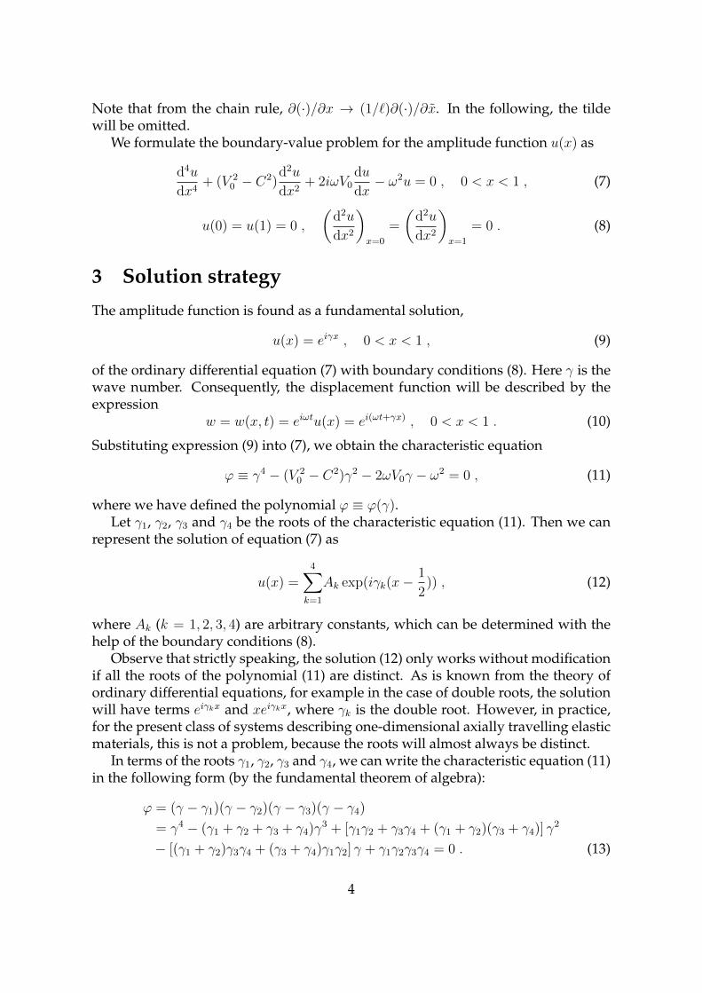
Figure 4: Example with C = 10. The natural frequency curves are the zero levelsets of the plotted expressions, with the exception of the seam between the real andimaginary regions (refer to subfigure (b)), where equation (30) is not valid. (a): Ex-pression g(ω, V0) = log(1+‖∆‖2). (b): Expressions log(1+[Re ∆]2) and log(1+[Im ∆]2).
0 2 4 6 8 10 12 14
- 100
- 50
0
50
100
v
ω
0
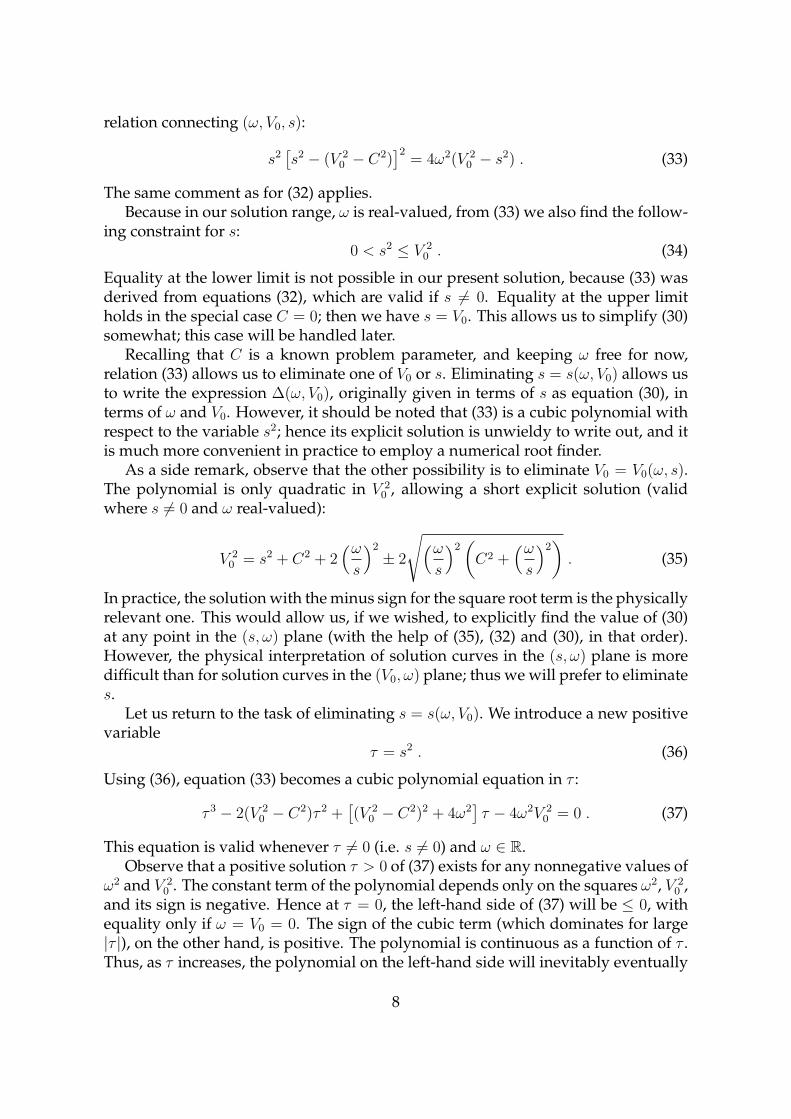
Figure 5: Zero-level set of (30) with C = 0, showing the four lowest natural fre-quencies ω as a function of panel velocity V0. Produced using the contour plotter ofMathematica, directly searching for the zero level set of the complex-valued expres-sion (41). Note good quality in most part of the plotting area, and accuracy problemsnear the V0 axis especially in the lowest mode.
17

0 2 4 6 8 10 12 14V0
0
20
40
60
80
100
120
140
160
ω
Figure 6: Four lowest natural frequencies ω as a function of panel velocity V0. Ten-sion load parameter C = 0.
The optimization process can be simplified into one input dimension, keeping V0fixed, or alternatively, keeping ω fixed. Another variant is to estimate the local tan-gent of the solution curve, and optimize parametrically in the direction orthogonalto it. The reduction to one dimension makes the optimization problem much eas-ier numerically, and also saves computational resources. However, a simple localoptimizer alone is not sufficient for this problem, because several branches of thesolution (zeroes of the complex norm) may reside in the plotting range, and all ofthem must be found.
Another approach to visualize the solution is to draw the zero level set of (30)using a contour plotter, but this requires very high accuracy and thus cannot begenerally recommended. See Figure 5 for an example in the case C = 0, using thespecial case formula (41).
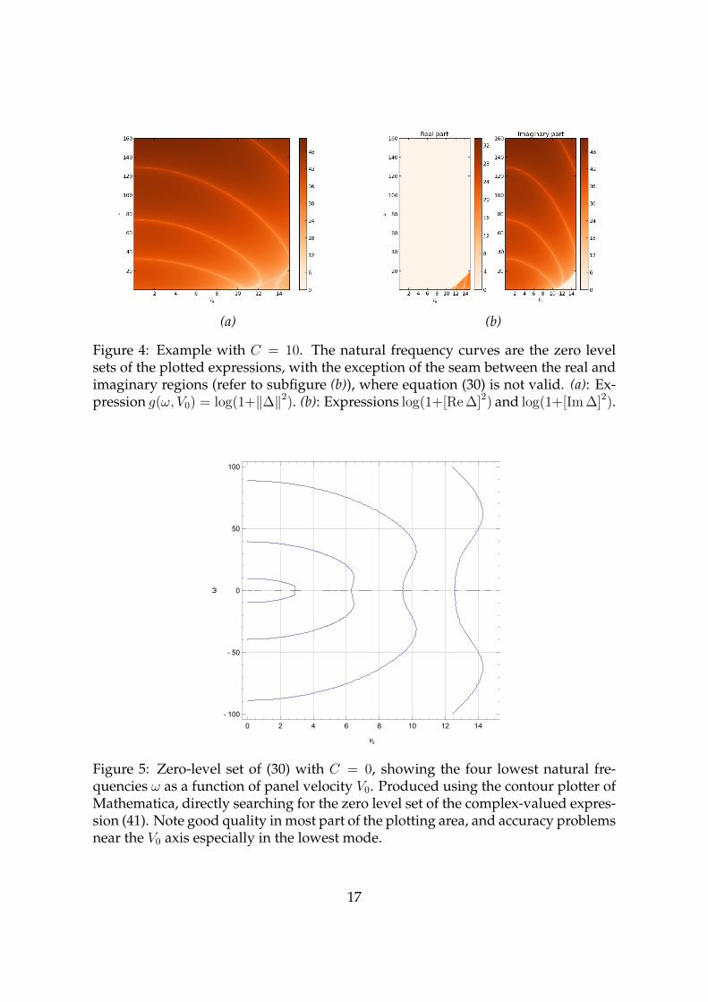
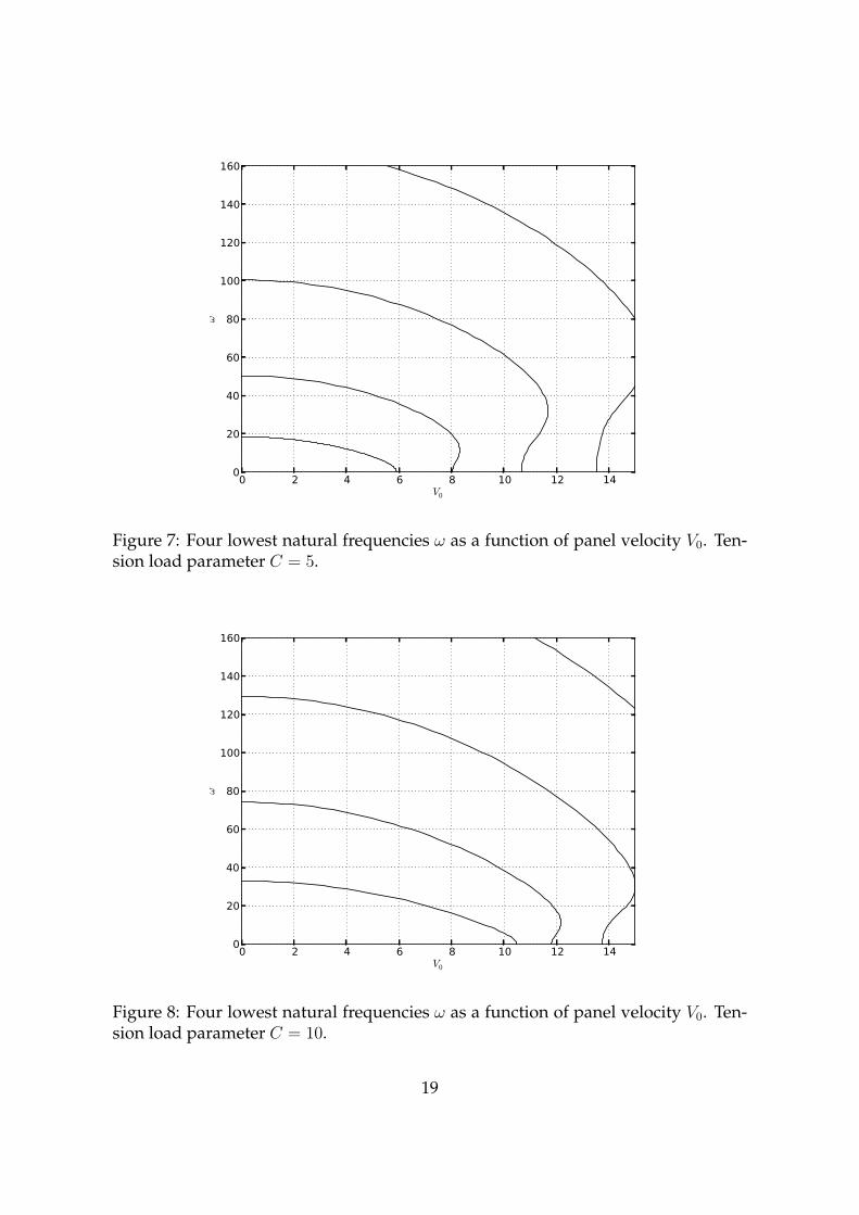
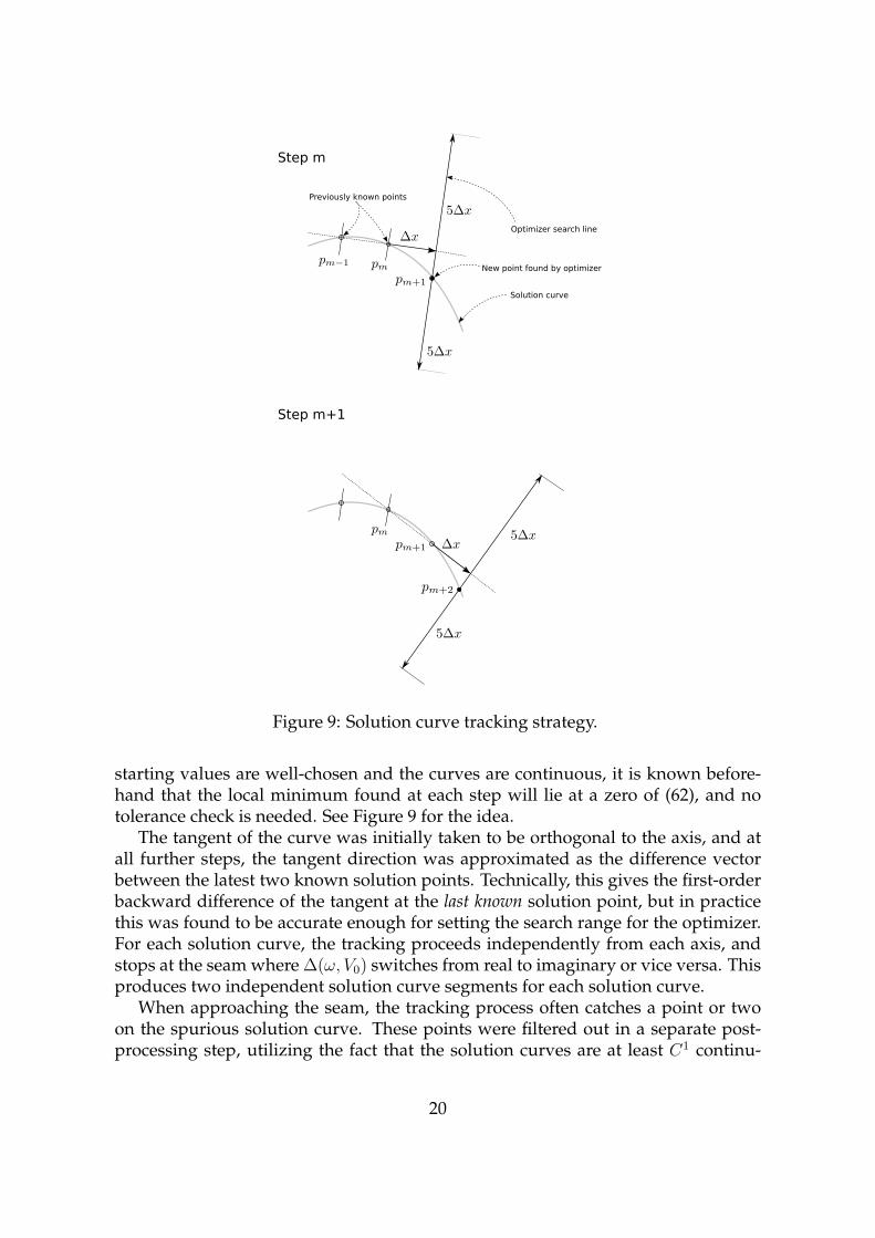
The final results for C = 0, C = 5 and C = 10 are shown in Figures 6–8, re-spectively. To produce these figures, we have first plotted (62) on a cartesian gridof 801× 801 points (as shown in Figures 2a–4a), and visually determined the pointswhere the solution curves cross the V0 and ω axes. Then, using these points as start-ing values, we have numerically tracked the solutions. For the purposes of tracking,the plot area shown in the figures was scaled to have square aspect ratio, and thetracking step size was set to 0.25% of plot area width.
Each solution point was obtained by local minimization of (62) along a boundedline segment orthogonal to the local tangent of the curve. The bounds for the op-timization were chosen as ±5 ∆x, where ∆x is the tracking step size. Because the
18
0 2 4 6 8 10 12 14V0
0
20
40
60
80
100
120
140
160
ω
Figure 7: Four lowest natural frequencies ω as a function of panel velocity V0. Ten-sion load parameter C = 5.
0 2 4 6 8 10 12 14V0
0
20
40
60
80
100
120
140
160
ω
Figure 8: Four lowest natural frequencies ω as a function of panel velocity V0. Ten-sion load parameter C = 10.
19
Solution curve
Optimizer search line
Step m
Step m+1
New point found by optimizer
Previously known points
Figure 9: Solution curve tracking strategy.
starting values are well-chosen and the curves are continuous, it is known before-hand that the local minimum found at each step will lie at a zero of (62), and notolerance check is needed. See Figure 9 for the idea.
The tangent of the curve was initially taken to be orthogonal to the axis, and atall further steps, the tangent direction was approximated as the difference vectorbetween the latest two known solution points. Technically, this gives the first-orderbackward difference of the tangent at the last known solution point, but in practicethis was found to be accurate enough for setting the search range for the optimizer.For each solution curve, the tracking proceeds independently from each axis, andstops at the seam where ∆(ω, V0) switches from real to imaginary or vice versa. Thisproduces two independent solution curve segments for each solution curve.
When approaching the seam, the tracking process often catches a point or twoon the spurious solution curve. These points were filtered out in a separate post-processing step, utilizing the fact that the solution curves are at least C1 continu-
20

ous. In practice, this was implemented as a difference-based local tangent check.Each vector of points (solution curve segment) produced by the tracking phase waschecked such that if the angle between the direction vectors determined by two suc-cessive point pairs (pm, pm−1) and (pm+1, pm) is more than 5 degrees, the points fromm + 1 onward (inclusive) are discarded and the postprocessing for that curve seg-ment ends. After both segments belonging to the same solution curve have beenpostprocessed, the segments are joined and plotted. The solutions behave smoothlyenough near the seam that linear interpolation (which the plotter performs) betweenthe last non-discarded points is accurate enough to produce a smooth-looking visu-alization (refer to Figures 6–8 for examples).
8 Conclusion
Analytical studies of the dynamic behaviour of moving elastic systems are very im-portant from both theoretical and practical points of view, and have attracted theattention of many researchers working in the domain of theoretical and applied me-chanics. Of particular interest has been the problem of elastic stability of a movingband and the application of dynamic analysis.
In the present study, in accordance with the dynamic approach of stability analy-sis, the problem of harmonic vibrations was investigated via the study of the depen-dences of the system’s natural frequencies on the problem parameters. Analyticalimplicit expressions for the solution curves, with respect to problem parameters,were derived for ranges of the parameter space where the natural frequencies arereal-valued, corresponding to stable vibrations. Both axially tensioned and non-tensioned travelling panels were considered.
The special cases of the non-tensioned travelling panel, and the tensioned sta-tionary (non-travelling) panel are also discussed, and special-case solutions given.Numerical evaluation of the obtained general analytical results was discussed, andnumerical examples were given for panels subjected to two different tension levels,and for the non-tensioned panel.
The performed analytical studies show in an explicit form the nature of the me-chanical instability for the travelling panel (and beam) model. The results allowthe development of very efficient, lightweight solvers for determining the naturalfrequencies of travelling panels and beams.
However, more importantly from the viewpoint of fundamental studies of axiallymoving materials, the results can be used to help locate the bifurcation points of thesolution curves, corresponding to points where mechanical stability is lost. By avariational argument, it is easily shown that at the bifurcation points, the tangent ofthe local branch of the solution curve in the (V0, ω) plane becomes vertical (Banichuket al., 2014a); the obtained analytical formulas can be used to help find such points.
AcknowledgementsThis research was supported by RFBR (grant 14-08-00016-a), RAS Program 12,
Program of Support of Leading Scientific Schools (grant 2954.2014.1), and the FinnishCultural Foundation.
21

References
F. R. Archibald and A. G. Emslie. The vibration of a string having a uniform motionalong its length. ASME Journal of Applied Mechanics, 25:347–348, 1958.
N. Banichuk, A. Barsuk, T. Tuovinen, and J. Jeronen. Variational approach for anal-ysis of harmonic vibration and stability of moving panels. Rakenteiden mekaniikka(Finnish Journal of Structural Mechanics), 47(4):148–162, 2014a.
N. Banichuk, J. Jeronen, P. Neittaanmaki, T. Saksa, and T. Tuovinen. Mechanics ofmoving materials, volume 207 of Solid mechanics and its applications. Springer, 2014b.ISBN: 978-3-319-01744-0 (print), 978-3-319-01745-7 (electronic).
V. V. Bolotin. Nonconservative Problems of the Theory of Elastic Stability. PergamonPress, New York, 1963.
L. Kong and R. G. Parker. Approximate eigensolutions of axially moving beamswith small flexural stiffness. Journal of Sound and Vibration, 276:459–469, 2004.URL http://dx.doi.org/10.1016/j.jsv.2003.11.027.
W. L. Miranker. The wave equation in a medium in motion.IBM Journal of Research and Development, 4:36–42, 1960. URLhttp://dx.doi.org/10.1147/rd.41.0036.
C. D. Mote. Divergence buckling of an edge-loaded axially moving band. Interna-tional Journal of Mechanical Sciences, 10:281–195, 1968a.
C. D. Mote. Dynamic stability of an axially moving band. Journal of the FranklinInstitute, 285(5):329–346, May 1968b.
C. D. Mote. Dynamic stability of axially moving materials. Shock and Vibration Digest,4(4):2–11, 1972.
C. D. Mote. Stability of systems transporting accelerating axially moving materials.ASME Journal of Dynamic Systems, Measurement, and Control, 97:96–98, 1975.
A. S. Mujumdar and W. J. M. Douglas. Analytical modelling of sheet flutter. SvenskPapperstidning, 79:187–192, 1976.
R. G. Parker. On the eigenvalues and critical speed stability of gyroscopiccontinua. ASME Journal of Applied Mechanics, 65:134–140, 1998. URLhttp://dx.doi.org/10.1115/1.2789016.
R. G. Parker. Supercritical speed stability of the trivial equilibrium of an axially-moving string on an elastic foundation. Journal of Sound and Vibration, 221(2):205–219, 1999. URL http://dx.doi.org/10.1006/jsvi.1998.1936.
A. Pramila. Sheet flutter and the interaction between sheet and air. TAPPI Journal,69(7):70–74, 1986.
22

A. Pramila. Natural frequencies of a submerged axially moving band. Journal ofSound and Vibration, 113(1):198–203, 1987.
W. H. Press and W. T. Vetterling. Numerical Recipes in Fortran 77: The Art of ScientificComputing. Cambridge University Press, 1992. ISBN 0-521-43064-X.
R. A. Sack. Transverse oscillations in traveling strings. British Journal of AppliedPhysics, 5:224–226, 1954.
A. Simpson. Transverse modes and frequencies of beams translating between fixedend supports. Journal of Mechanical Engineering Science, 15:159–164, 1973. URLhttp://dx.doi.org/10.1243/JMES JOUR 1973 015 031 02.
R. Skutch. Uber die Bewegung eines gespannten Fadens, weicher gezwungen istdurch zwei feste Punkte, mit einer constanten Geschwindigkeit zu gehen, undzwischen denselben in Transversal-schwingungen von gerlinger Amplitude ver-setzt wird. Annalen der Physik und Chemie, 61:190–195, 1897.
A. Thurman and C. Mote, Jr. Free, periodic, nonlinear oscillation of an axi-ally moving strip. Journal of Applied Mechanics, 36(1):83–91, Mar. 1969. URLhttp://dx.doi.org/doi:10.1115/1.3564591.
S. P. Timoshenko and S. Woinowsky-Krieger. Theory of plates and shells. New York :Tokyo : McGraw-Hill, 2nd edition, 1959. ISBN 0-07-085820-9.
Y. Wang, L. Huang, and X. Liu. Eigenvalue and stability analysisfor transverse vibrations of axially moving strings based on Hamil-tonian dynamics. Acta Mechanica Sinica, 21:485–494, 2005. URLhttp://dx.doi.org/10.1007/s10409-005-0066-2.
J. A. Wickert and C. D. Mote, Jr. On the energetics of axially moving con-tinua. The Journal of the Acoustical Society of America, 85(3):1365–1368, 1989. URLhttp://link.aip.org/link/?JAS/85/1365/1.
23