Embed Size (px)
DESCRIPTION
slab moment under point load
Citation preview
, Yr:2C;~ ~/ ~6'2q;/
l
l .
·l
CIVIL- ENGINEERING STUDIES C!OfJ· ~UCTURAL. RESEARCH SERIES NO. 264
ANALYTICAL STUDY F E ENTS
IN C NTINU US SLABS SUBJECTE
T C NCENTRATE LADS
Yetz Reference Room . E "Tloering Department
Ci v~l ngJ.. .. v. • 0-
'B106 c. E. }3Ullcllr:o °
. °ty of IlllnolS Unlvers~ 1
I llinois 6180 Urbana,
By R. E. WOODRING
and
c. P. SIESS
UNIVERSITY OF ILLINOIS
URBANA, ILLINOIS
MAY 1963

AN ANALYTICAL STUDY OF THE MOMENTS
IN CONTINUOUS SLABS SUBJECTED
TO CONCENTRATED LOADS
By
R • E G Wood r i n 9
and
C. P. Siess
Un i ve rs i ty of 111 i no is
Urbana, Illinois
May 1963

... iii ...
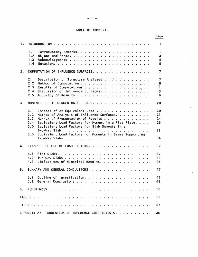
TABLE OF CONTENTS
10 INTRODUCTION. 0 • 0 0 • 0 0
1.1 Introductory Remarkso 0
1.2 Object and Scope. 0 0 0 0 0 0 • 0 ..
103 Acknowledgments 0 0 0 0 0 0 0 0 •
104 Notationo 0 0 0 0 0
20 COMPUTATION OF INFLUENCE SURFACESo
201 Description of Structure Analyzed 0
202 Method of Computat ion 0 0 • 0 0 0 0
203 Results of Computations 0 0 0 0 0
204 Discussion of Influence Surfaces. 205 Accuracy of Results 0 0
MOMENTS DUE TO CONCENTRATED LOADSo 0
• 0' 0 • e 0
o 0,
·0 . ,0 .0 . G
301 Concept of an Equivalent Load 0 0 0 0 0 0 0 0
302 Method of Analysis of !nfluence Surfaceso 303 Manner of Presentat i on of Resu 1 ts 0 0 Q .. 0 • 0 0
40
304 Equivalent Load Factors for Moment in a Flat Plate. 305 Equivalent Load Factors for Slab Moments in a
Two-Way Slab 0 0 0 0 0 0 0 0 0 0 0 0 0 0 0 0 0 0
306 Equivalent Load Factors for Moments in Beams Supporting Two-Way Slabs 0 0 0 0 0
EXAMPLES OF USE OF LOAD FACTORSo 0 0 0 0 0 0
40 1 Flat Slabso 0 0 0 0 0 0 0 0 0 0 0 0 0 . 0 0 0 0 0 0
402 Two-Way Slabs 0 0 0 0 0 . 0 0 0 0 Q
4.3 Lim i tat ions of Numer i cal Resultso 0 0 0 0 0 0
5. SUMMARY AND GENERAL CONCLUSIONSo
501 Out1 ine of investigationo 502 General Conclusions
.. 0
0
60 REFERENCES 0 o 0 0008000
TABLES 0 0 0
FIGURES 0 •
APPENDIX A~ TABULATION OF ~NFLUENCE COEFF~CIENTSo o 0 0
1 3 5 5
7
7 .. 8
'. "1' '1
13 16
20
20 21 24 26
31
34
37
37 42 45
47
47 48
50
51
57
136
- iv'"
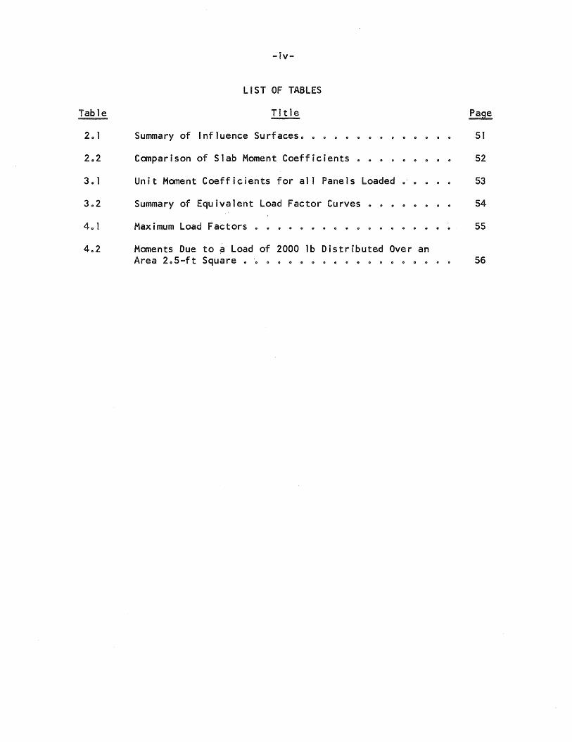
LIST OF TABLES
Table Ti tle
Summary of Influence Surfaceso II 0 51
2 .. 2 Comparison of Slab Moment Coefficients. 52
30 1 Unit Moment Coefficients for all Panels Loaded 53
Summary of Equivalent Load Factor Curves .. 54
Maximum Load Factors .. 0 o 0 0 fiI 55
Moments Due to ~ Load of 2000 lb Distributed Over an Area 2 .. 5-ft Square 1/ '0 .. 0 0 .. 0 .. 0 0 0 0 0 .. 0 0 0 56
Figure
2,,2
2,,3
2 .. 8
2" 11
2 .. 14
-v-
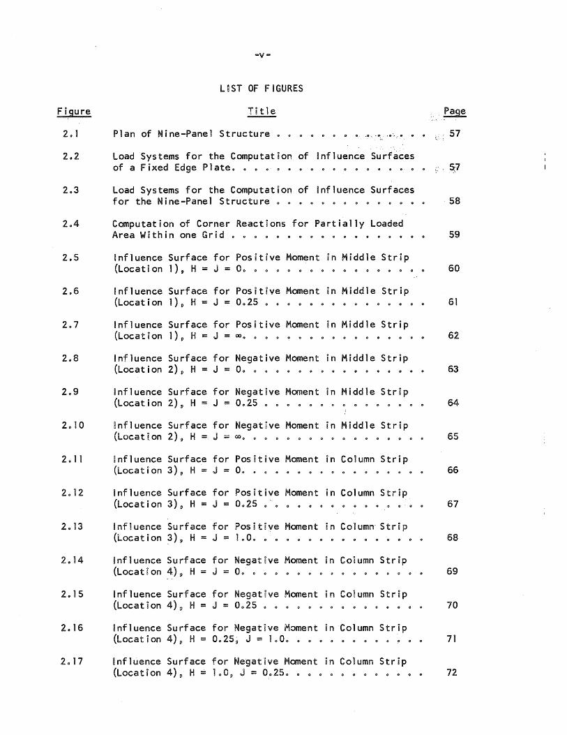
LIST OF FIGURES
Title
Plan of Nine-Panel Structure 0 0 o 0 0 0 0 0.- .~_. "0;. lO::,:O 0 0
Load Systems for the Computation of ~nfluence Surfaces of a Fixed Edge Plate" 0 0 0 0 0 0 Q 0 0 0 0 0 0 0 0 0 0
Load Systems for the Computation of Influence Surfaces for the Nine-Panel Structure 0 0 0 0 0 0 0 0 0 0 0 0
Computation of Corner Reactions for Partially Loaded Area Within one Grid 0 0 0 0 0 0 0 " 0 0 0 0 0 0 0 0
Influence Surface for Positive Moment in Middle Strip (Location 1), H = J = 00 0 0 0 0 0 0 0 0 0 0 0 0 " 0 0 0
influence Surface for Positive Moment in Middle Strip (Location l)p H = J = 0025 0 0 0 0 0 0 0 0 0 0 0 0 0 0 0
Influence Surface for Positive Moment in Middle Strip (Location l)p H = J = 00 0 0 0 0 0 0 0 0 0 0 0 0 0 0 0 0 ..
Influence Surface for Negative Moment in Middle Strip (Location 2)9 H = J = 00 0 0 0 0 0 0 0 0 0 0 0 0 " 0 a 0
Influence Surface for Negative Moment in Middle Strip (Location 2)9 H = J = 0025 0 0 0 0 0 0 0 0 0 0 0 " 0 0 0
~nfluence Surface for Negative Moment in Middle Strip (Location 2)9 H = J = 00 0 0 0 0 0 0 0 0 0 0 0 0 0 0 0 0 0
Influence Surface for Positive Moment in Column Strip (Location 3)9 H = J = 00 0 0 0 0 0 0 0 0 0 0 0 0 0 0 0 0
Influence Surface for Positive Moment in Column Strip (Location 3)9 H = J = 0025 0 0 0 0 " 0 0 0 0 0 0 0 0"" 0
influence Surface for Positive Moment in Column" Strup (Location ~)9 H = J = 1000 0 0 0 0 0 0 0 0 0 0 0 0 0 0 0
influence Surface for Negatove Moment in Column Strip (Location 4)9 H = J = 00 0 0 0 0 0 0 0 0 0 0 0 0 0 0 0 "
influence Surface for Negatove Moment in Column Strop (Location 4)p H = J = 0025 0 0 0 0 0 0 0 0 0 0 0 0 0 0 ..
2016 Influence Surface for Negative Moment in Column Strip
2" 17
(L oc a t i on 4 L, H = 00 2 5 ~ J = 1 0 00 0 0 0 0
Influence Surface for Negative Moment in Column Strip (Location 4)p H = loOp J = 00250 0 0 0 0 0 0 0 0 0 0 0 0
c: 57
5}
58
59
60
61
62
63
64
65
66
67
68
69
70
71
72
-v i ...
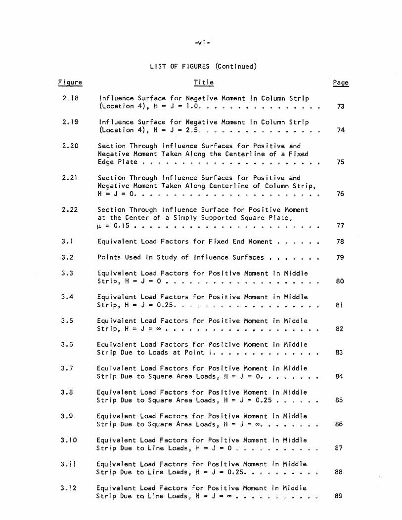
l~ST OF FIGURES (Continued)
Figure Title
Influence Surface for Negative Moment in Col umn Strip '(Locat ion 4L) H = J = 1000 0 0 0 0 0 0 0 0 0 0 0 0 0 0 0
Influence Surface for Negative Moment in Column Strip (Locat i on 4), H = J = 2050 0 0 0 0 0 0 0 0
2020 Section Through influence Surfaces for Positive and Negative Moment Taken Along the Centerl ine of a Fixed Edge Plate 0 0 0 0 0 0 0 0 0 0 0 0
2021 Section Through ~nfluence Surfaces for Positive and Negative Moment Taken A10ng Center] ine of Column Strip,
301
3 .. 4
3.8
3010
3 .. 12
H = J = 00 0 0 0 0 0 0 0 0 0 0 e 0 0 0
Section Through Influence Surface for Positive Moment at the Center of a Simply Supported Square Plate p
IJ. = 00 15 <> 0 0 0 0 0 0 0 0 0 0 I) 0 0 0 0 0 0 o 0 •
Equivalent Load Factors for Fixed End Moment 0 0
Points Used in Study of ~nfluence Surfaces 0 0
Equivalent load Factors for Positive Moment in Middle Strip, H = J = 0 0 0 .. 0 0 0 0 0 0 g 0 0 0 0 .. 0 0 0 0 0
Equivalent Load Factors for Positive Moment in Middle StroP9 H = J = 00250 0 0 0 0 0 0 0 0 0 0 0 0 0 0 0 0 0 0
Equivalent load Factors for Positive Moment on Middle Strip!) H = J = 00 .. 0 0 0 0 0 0 0 0 0 0 II 0 0 0 0 0 0 0 0
Equivalent load Factors for Positive Moment in Middle Strip Due to loads at Point ~o 0 0 0 .. 0 0 0 0 0 0 0 0 0
Equivalent load Factors for Pos~tive Moment in Middle Strip Due to Square Area loads!) H = J = 00 0 0 0 0 0 0 0
Equivalent load Factors for Positive Moment in Middle Strip Due to Square Area loads p H = J = 0025 0 0 0 0 0 0
Equivalent load Factors for Positive Moment in Middle Strip Due to Square Area loads!) H = J = ~o 0 0 0 0 0 0
Equivalent load Factors for Positive Moment in Middle Strip Due to Line loads!) H = J = 0 0 0 0 0 0 0 0 0 0 0 0
Equ6valent load Factors for Positive Moment an Middle Strip Due to Line Loads p H = J = 00250 0 0 0 0 0 0 0 0 0
Equivalent load Factors for Positive Moment ~n Mndd1e S t rip Due to line Loads!) H = J = ~ 0 0 0 0 0 0 0 0 0 0 0
73
74
75
76
77
78
79
80
81
82
83
84
85
86
87
88
89
-v n i-
LIST OF F~GURES (Continued)
Figure Tn tie Pag.e
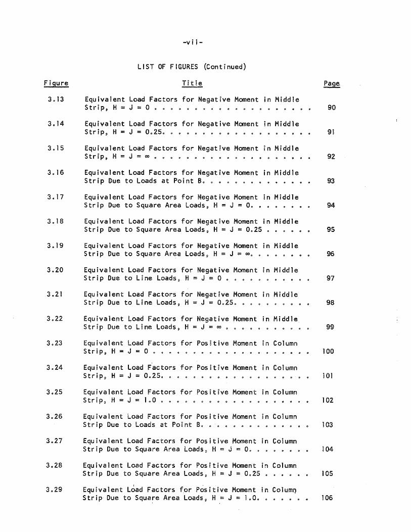
Equivalent Load Factors for Negative Moment in Middle Strip, H = J = 0 0 0 0 0 0 .. 0 0 ...... 0 0 0 0 0 .... 0" 90
Equivalent Load Factors for Negative Moment in Middle Strip, H = J = 00250 0 .... 0 .. 0 0 0 0 0 0 0 0 0 .. 0 0" 91
Equivalent Load Factors for Negative Moment in Middle Strip, H = J = 00 0 0 0 0 0 0 0 0 0 0 0 0 0 0 0 0 0 .. .... 92
Equivalent Load Factors for Negative Moment in Middle Strip Due to Loads at Point 80 0 ...... 0 .. 0 0 0 0 0 .... 93
3. 17 Equivalent Load Factors for Negative Moment in Middle Strip Due to Square Area Loads, H = J = 00 .... 0 .. 0 0 0 94
Equivalent Load Factors for Negative Moment in Middle Strip Due to Square Area Loads, H = J = 0025 0 0 0 0 .... 95
3" 19 Equivalent Load Factors for Negative Moment in Middle Strip Due to Square Area loads, H = J = 00 0 .. 0 0 0 .. .... 96
3 .. 20 Equivalent Load Factors for Negative Moment in Middle Strip Due to Line loads, H = J = 0 0 0 .. 0 0 0 0 0 0 .... 97
3 .. 21 Equivalent Load Factors for Negative Moment in Middle Strip Due to Line Loads!) H = J = 00250 .. 0 0 0 0 0 0 0 0 98
Equivalent load Factors for Negatuve Moment in Middle Strip Due to lane Loads, H = J = 00 .. 0 0 .. 0 .... 0 0 0.. 99
Equivalent load Factors for Positive Moment in Column Strip, H = J = 0 0 .. 0 0 0 0 0 0 0 0 0 0 0 0 0 0 0 .. 0.. 100
3 .. 24 Equivalent load Factors for Positive Moment in Column Strip, H = J = 00250 0 0 0 0 0 0 .. " 0 0 0 0 0 0 0 00 0 101
3.25 Equivalent Load Factors for Positive Moment in Column Strip, H = J = 100 0 0 0 0 0 0 0 .. 0 0 0 0 0 .. 0 0 0 .. 0 102
3 .. 26 Equivalent Load Factors for Positive Moment in Column Strip Due to loads at Poont Bo 0 0 0 .. 0 0 0 0 .... 0 0 0 103
Equivalent load Factors for Positive Moment in Column Strip Due to Square Area Loads v H = J = 00 0 0 0 ...... 0 104
3028 Equivalent load Factors for Positive Moment in Column Strip Due to Square Area Loads o H = J = 0025 0 0 0 0 0.. 105
I '
Equivalent load Factors f,6r Positive Moment in Columr) Strip Due to Square Area loads, H = J = ioOo 0 0 0 .. 0 0 106
"'v i i 6 ...
LIST OF FIGURES (Continued)
Title Page
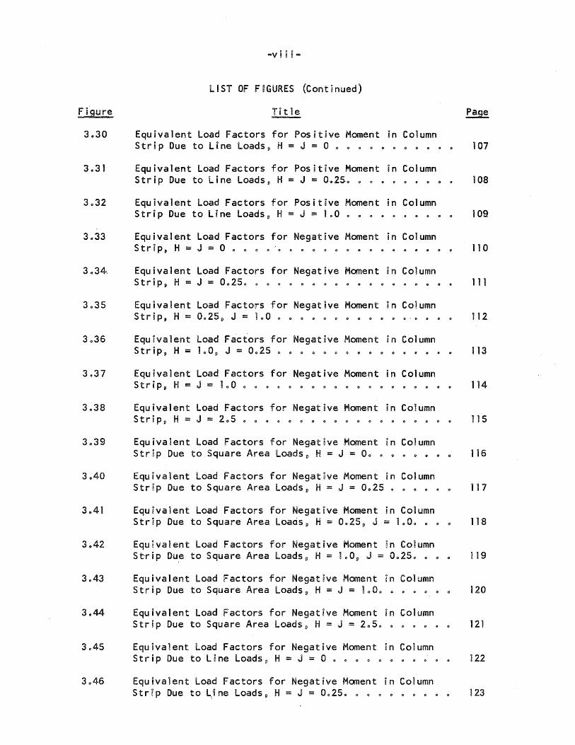
3 .. 30 Equivalent Load Factors for Positive Moment in Column Strip Due to line Loads 9 H = J = ° 0 0 0 0 0 0 0 0 0 0 0 107
Equivalent Load Factors for Positive Moment in Column Strip Due to Line Loads, H = J = 0 .. 25-0 0 0 0 0 0 0 0 0.. 108
Equivalent load Factors for Positive Moment in Column Strip Due to Line loads 9 H = J = 100 0 0 0 0 0 0 0 0 0 0 109
Equivalent Load Factors for Negative Moment in Column Strip, H = J = 0 0 0 0 0 0 0 0 0 0 0 0 0 0 0 0 0 0 .. 0 0 110
Equivalent Load Factors for Negative Moment in Column Strip, H = J = 00250 0 0 0 0 0 0 0 0 0 0 0 0 0 0 0 0 0 0 111
Equivalent Load Factors for Negative Moment in Column Strip, H = 0025 9 J = ioO 0 0 0 0 0 0 0 0 0 0 0 o· 0 • 0 0 J12
Equivalent load Fact'ors for Negative Moment in Column Strip9 H = laO!) J = 0025 0 0 0 0 0 0 0 0 0 0 0 0 0 0 0 0 113
Equivalent load Factors for Negative Moment in Column Strip9 H = J = 100 0 0 0 0 0 0 0 0 0 0 0 0 0 0 0 0 0 0 0 114
Equivalent Load Factors for Negative Moment in Column Strip9 H = J = 205 0 0 0 0 0 0 0 0 0 0 0 0 0 0 0 0 0 0 0 115
Equivalent load Factors for Negat~ve Moment in Co1umn Strip Due to Square Area loads o H = J = 00 0 0 0 0 0 0 0 116
Equivalent load Factors for Negatnve Moment in Column Strip Due to Square Area loads!) H = J = 0025 0 0 0 0 0 0 117
Equivalent Load Factors for Negative Moment in Column Strip Due to Square Area loads g H = 0025 9 J = 1000 0 0 0 118
3 .. 42 Equivalent load Factors for Negative Moment ~n Column St-rip Due to Square Area loads!) H = 1001) J = 00250 0 0 0 119
Equivalent load Factors for Negative Moment in Column Strip Due to Square Area loads!) H = J = ~oOo 0 0 0 0 0 0 120
3.44 Equivalent load Factors for Negative Moment in Column Strip Due to Square Area loads D H = J = 2050 0 0 0 0 • 0 121
Equivalent Load Factors for Negative Moment in Column Strip Due to Line loads!) H = J = 0 0 0 0 0 0 0 0 0 0 0 0 122
Equivalent Load Factors for Negative Moment in Column Strip Due to LJne Loads 9 H = J = 00250 0 0 0 0 0 0 0 0 0 123
Figure
3 .. 47
3 .. 50
3 .. 51
3 .. 52
3 .. 54
4.1
4 .. 2
4 .. 3
4 .. 4
4.5
"'ix ...
liST OF FIGURES (Continued)
Title
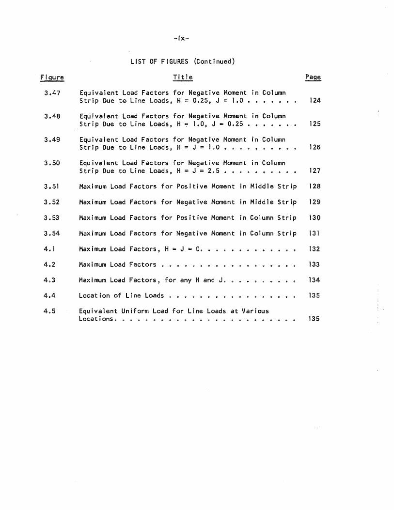
Equivalent load Factors for Negative Moment in Strip Due to line Loads, H ::: 0025, J ::: 1.0 ....
Equivalent load Factors for Negative Moment in Strip Due to line loads, H ::: loOp J ::: 0.25 0 •
Col umn .. 0 0 0 ..
Col umn .. 0 . .. ..
Equivalent Load Factors for Negative Moment in Column Strip Due to line Loads p H ::: J ::: 100 ... 0 0 ......... $
Equivalent load Factors for Negative Moment in Column Strip Due to line loads, H ::: J ::: 205 .. 0 ..
Maximum load Factors for Positive Moment in Middle Strip
Maximum load Factors for Negative Moment in Middle Strip
Maximum load Factors for Positive Moment in Column Strip
Maximum load Factors for Negative Moment in Column Strip
Maximum load Factors 9 H ::: J ::: 0 .. CIt 0 • •
Maximum load Factors ...... 0 0 0 0 o ..
Maximum Load Factors, for any Hand Jo .. 0 0 .. 0 0
location of line loads 0 0 0 .. 0
Equivalent Uniform Load for Line Loads at Various Locations .... 0 0 0 0 0 0 0 0 .. 0 .. 0 0 0 0 0
Page
124
125
126
127
128
129
13Q
131
132
133
134
135
135
... x-
L~ST OF TABULATIONS ~N APPENDIX A
Figure Title Page
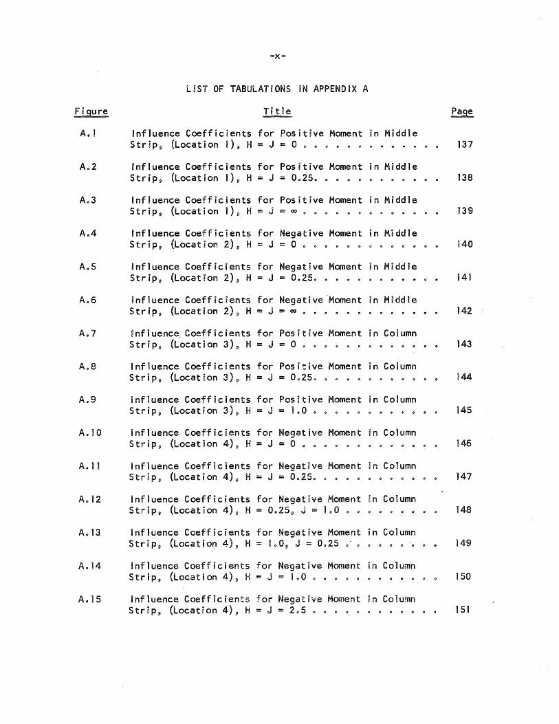
Ao 1 Influence Coefficients for Pos it ive Moment in Middle Stripll (Locat ion I ) 11 H = J = 0 0 0 0 0 0 0 0 0 0 0 " 137
Ao2 Influence Coefficients for Positive Moment in Middle Strip, (Locat ion 1 ) !) H = J = 00250 0 0 0 0 0 " " .. 0 138
A,,3 Influence Coefficients for Positive Moment in Middle Strip, (locat ion 1 L) H = J =00 0 0 0 0 " 0 0 0 0 0 0 139
Ao4 Influence Coefficients for Negative Moment in Middle Strip9 (locat ion 2) 11 H = J = 0 0 0 0 0 0 0 0 0 0 0 .. 140
Ao5 Inf1uence Coefficients for Negative Moment in Middle Strip, (locat ion 2) l) H = J = 00250 0 0 0 0 " .. 0 " 0 141
A.6 influence Coefficients for Negative "Moment in Middle Strip9 (locat ion 2) l) H = J = co 0 " 0 0 0 0 0 " 0 0 0 142
Ao7 ~nfluenc~ Coefficients for Positive Moment in Column Strip9 (locat i on 3) I) H = J = 0 0 0 0 0 0 0 0 0 0 0 0 143
Ao8 Influence Coefficients for Positive Moment in Column StriPll (Locat 6 on 3) l) H = J = 00250 0 0 0 0 0 0 0 0 0 144
A.9 ~nf1uence Coefficients for Positive Moment in Column Stripll (loea t i on 3) l) H = J = 1.,0 0 0 0 0 0 0 " 0 0 " 145
Ao 10 influence Coefficients for Negative Moment un Column Stripl) (locat ion 4) l) H = J = a 0 0 0 0 " " 0 0 0 " 0 146
A 0 11 influence Coefficients for Negatnve Moment in Column Strip!) (locat i on 4) 11 H = J = 00250 0 0 0 0 0 0 0 0 0 147
Ao 12 Influence Coefficients for Negative Moment in Column Strip!) (locat 8 on 4) 9 H = 0025 9 J = 100 " 0 .. " 0 0 .. 0 0 148
Ao 13 Influence Coefficients for Negative Moment in Column Stripv (locat ion 4) v H = 1 00 v J = 0025 " .. 0 0 0 0 0 " 0 149
Ao 14 Influence Coefficients for Negatove Moment in Coiumn Strip9 (locat B on 4) l) H = J = 100 0 0 0 0 0 0 " 0 . Q 150
Ao 15 ~nfluence Coeffocoents for Negative Moment in Column StraP9 (location 4) l) H = J = 205 0 0 0 0 0 0 0 0 0 0 151
10 ~NTRODUCT~ON
101 Introductory Remarks
The moments in reinforced concrete floor slabs continuous in two
directions and subjected to loads not distributed over an entire panel are
usually computed using equivalent ]oads distributed uniformly over the entire
panel area o The equivalent un~formly distributed loads are sometimes
specified by building codes s but more often are left to the judgment of the
designero For exampleD it ~s commonly assumed nn desngning a slab that a
load of 30 psf uniformly distrnbuted over the entire panel 8S sufficient to
take care of loads from part~toonsD wh~ch are actually 1 ine loadso it is
doubtful if the same uniformly d~strnbuted load apploes for all the critical
moments in a slab as wel] as for al] of the possible sizes and locations of
partitionso In some cases the use of an equiva!ent uniform load may be
conservative for the moment at one ]ocation nn a slab yet unconservative
for the moment at another locatnono Partit~on loads are just one example
of concentrations of loado Other examples are wheel loads from vehicles
in parking garages o wheel loads from fork iift trucks in manufacturing
buildings or warehouses p and heavy machinery loads dnstributed over small
areaso
The requirements of most building codes (1) with regard to
concentrations of load on floor s1abs are concerned w~th the types just
mentionedo One of the most common prOV8SftOnS 8S for a load of 20000 lb to
be spread over an area of 205 ft sq located to produce maximum stress
conditions in the structural member 0 A common provision for parking
garages is the use of a uniformly distributed live ]oad of 100 ib per sq
ft or tso percent of the maximum whee~ load p]aced anywhere on the flooro
-2-
Although it is obv ious that moments due to concentrated loads need
to be considered in the design of most floor slabs!) the complexity of the
necessary analysis makes the computation of such moments difficult and
impractical 0 Hence, in most cases, computations are based on equivalent
uniform loads over the entire panel, which mayor may not yield consistent
or correct resultso
The most convenient way of finding moments due to concentrated
loads or loads distributed over small areas is by the use of influence
coefficients or, more conveniently, by the use of influence surfaces
constructed from such coefficientso Influence surfaces for slabs are
analogous to influence lines for beamso With their use!) critical moments
at particu1ar points in the slab can be found for any position of the load
or extent of the loaded areao
Influence surfaces based on the theory of medium thick plates are
available in the literature for various ·types of support conditionso
A.Pucher (2) has published 81 influence surfaces for bending moments p
twisting moments g and shears at selected points in isolated single panels
having various combinations of fixed!) simply-supported!) and free edge
conditionso Go Hoeland (3) developed influence surfaces for moment in the
slab over an interior rigid support in two span contenuous plates having
various combinations of fixed, simply-supported!) or free edge conditions
and various aspect ratioso Eo Ho R~sch and Ao Hergenroder (4) obtained
influence surfaces by model analysis for isolated single panel skew slabs
which have various aspect ratios and skew angles and which are simply
supported on opposite edges and free on the other edges!) Vo Po Jensen (5),
No Mo Newmark and Co Po Siess (6) obtained influence surfaces for moments
in the slabs and beams of single span haghway bridgeso Thes~9 however,
-3 ....
are not appl icable to floor slabs continuous in two directions because they
consider the main span simply supportedo Thus g there are no influence
surfaces available in the literature for floor slabs wh~ch 'take into account
deflection and rotation of the boundaries as well as continuity with other
panels in both directionso
102 Object and Scope
The object of this investigation was to study the moments in
interior panels of continuous floor slabs subjected to concentrated loads
or loads distrjbuted over a portion of the pane) areao The investigation
was carried out in three phaseso Furst p influence surfaces were computed
for the interior panel in the array of nine square panels shown i.n Figo 20 L
Second, a study was made of influence surfaces to determine the significant
variableso And final1Y9 criteria for the calcutatoon of moments in slabs
subjected to concentrated loads were formulatedo Because of the limited
scope of the analysis 9 these criteria are more iitustrat~ve than general
but stull may be useful in designo
The nine .... panel structure was used in this study because a computer
program for its analysis was already availabieo This program p which was
coded for the ILLIAC p one of the electronic computers at the University of
illinois, utilizes a numerical procedure based essentially on finite dif
ferences to analyze a mathematnca] model of the structureo This numerical
procedure takes unto account both flexural and torsional stiffness of the
supporting beams. By studying the interior pane1 of the nine-panel
structure, account was taken of cont~nu~ty in two directions.
Table 2.1 summarizes the cases for which snfluence surfaces were
computed 0 By considering the supporting beams to have zero flexural and
tor,sional-S.t.lff~ll the nine,"'panel structure has. no beams an.d.ls, . ..repr.e~
sen.tative of, the type. of f100r construction known·· 'as the IIflat pla.teUlg
whi.ch-· is similar to the flat slab but without drop panels or -c~pital.so
When the ·beams·.are cons ider.ed to· have st.iffness 11 the structur..e . ..ana,lyzed is.
similar to the .type ~f floor commonly called iltwo-wa.y systemssupp.orted on
four sides"!) or simply a two-way s1.ab'(I For this type of structure 9 the
influence surf.aces wer·e broken down into two groups; those for slab moments
and those fo.r beam. moments 0 On 1 y two corm i nat ions of f 1 exur.al and tors i ona]
stiffness were consi . .dered for slab moments wh~le five combinations of
f 1 exu.ra.1 and. tors i ona 1 s t if fness were cons i dered for beam momen ts 0
Influence coeffi.cients were computed and anfluence surfaces drawn
for moments at four locations in the slab as shown in Figo 2010 The locati.ons
corr,e.spond generally to the critical sections considered in the design of
floor slabso Influence coefficients were obtained for moments so. the
beams at locations corresponding to those marked 3 and 4. in FiSo 2010
The study of influence surfaces to determine the sign.ificant
variables was made by considering area loads centered at nine different
points in the paneJo The locations of these points are shown in Figo 3020
The loads included a singl~~oncentrated load at the point p line loads
through the point in both directions parailelto the edges of the panel,
and loads distributed over rectangular areas extending up to one-third
the span length in each darectiono
The results have been enterpreted and made suitable for practical
uses by ~ntroducing the concept of equivalent panel loads which!) when used
with conventional code procedures p give: an effect equal to that of the load
distributed over a small areao The equivalent panel load of course varies
-s ...
in magnitude with the type of floor system g location of moment, location of
load, and extent of loaded areao
The analysis has 1 imited appl ication to reinforced concrete since
it assumes elastic behavior of the structureo However 9 the precedent for
using this type of analysis is well establ ished since a more accurate method
of analysis which takes account of creepg shrinkage p and cracking of the
concrete has not yet been developedo in addition to the assumption. of
elastic behaviorp the numerical procedure used in the computations is based
on finite difference equationso However s ssnce a fine network of 400
squares was used p the approximatoon is quite good in most caseso
103 Acknowledgments
This thesis was prepared under the direction of Oro Co Po Siess s
- Professor of Civil Engineerongo The author expresses his appreciation
for the guidance and helpful advice gnven by Professor Siess during the
progress of thIs investogatoono Additional help was given by Oro Ao Ang 9
Associate Professor of Civil Engineerang D in connection with the computations
carried out on iLLiACo The author wishes to express his appreciation for
Professor AngDs assostanceo
104 Notation
a = distance fram support to the resultant load
C = equivalent load factor
c = constant desognating size of column
d = diameter of small circularly loaded area
Eb = modulus of e·lastacity of the beam material
E = modulus of elasticity of the slab material in a particular panel
.... 6 ...
Eb Gb = 2(1 + J..I.) shear modulus of elasticity of the beam material
Eb1b H - ---- ratio of beam flexural stiffness to slab stiffness -Nl
h = height of partition
Ib = moment inertia of the cross-section of a beam
J = ~~ ratio of beam torsional stiffness to slab stiffness
K = a measure of the torsBonal rig~dity of a beam cross-section
(See Ref 0 7)
kpkxp ky = constants defining the size of an area or line load
l = span length of one panel 9 center to center distance between
col umns
m = bending moment per unit width of slab produced by a concentrated
load
mB = unit moment produced by loading all nine pane1s
P m = 8d/l 0 2032 + Oo049P unit moment directly under a concentrated
load
N Et3
- 2 12...(1 ... I-l ) measure of the plate stiffness ~n a particular panel ..
P = concentrated load
q = uniformly distributed load per un,Jt of ,.area
t = thickness of slab
W = a load dis t r n bu ted ove r an a rea
w = vertical deflectuon of the slab
w = unit weight of a partition
Xp Y = rectangular reference coordinates
Op ~ = constants defining the location of the resultant load within
a grid space
~ = distance between node points of grid
J..I. = PoissonBs ratio
-7-
20 COMPUTATiON OF ~NFlUENCE SURFACES
201 Description of Structures Anaiyzed
The plan of the structures ana1yzed ~n this investigation is shown
in Figo 2010 It cons ists of nine square panels arranged three by threeo
The slab is of uniform thicknesso _ The columns have a c/l ratio of 001 and
are assumed to be infinitely st~ff ~n flexure and to provide non-deflecting
supports to the slabo The structure is assumed to be made of an elastic,
homogeneous~ isotropic material wHth Ponssonis ratio assumed to be zeroo
The stiffness of the beams spanning between columns is related to the
stiffness of the slab g using the dimensionless parameters Hand Jo H is a
measure of flexural stiffness of the beam related to the stiffness of the
slab and is defined as~
(201 )
where: Eb = modulus of elastncsty of the beam maternal
Ib = moment of anertia of the cross-section of a beam
Et3 N = -----~--~ = a measure of the stiffness of the plate in a
12(1 - 1l2
)
particular panel
E = modulus of elasticity of the slab material an a particular
panel
t = thickness of slab
~ = PoissonDs rat~og taken as zero fin this investigation
l = span length of one panel
J is a measure of the torsional stoffness of the beam re]ated to the
stiffness of the slab and os defined as~
J = GK Nl
-8-
where: Eb
G = 2(1 + ~) = shear modulus of elasticity of the material in a
beam
b3d K = --3- f] = a measure of the torsional rigidity of a beam cross-
section (See Refo 7)
The different values of Hand J used in this investigation are
summarized in Table 2010 The case of H = J = 0 is of considerable inte~est
since the beams spanning between the columns have no stiffness and the
structure represents the type of f100r construction which is known as the
Blflat plateil which is similar to the flat slab but without capitals or
drop pane1so Where Hand J have finite values 9 the structure analyzed is
similar to the type of floor system commonly called Ditwo-way system
supported on four sides BI or simply a two-way slab"
The case of H = J = 205 is representative of the flexural and
torsional stiffnesses of deep reinforced concrete beams which are designed
using current code requirements whereas beams having H = J = 0025 are
quite flexible and are representative of much smaller supporting beams.,
202 Method of Computation
Finite difference equations are the basis for the computations
made in this investigationo No Mo Newmark (8) has described a procedure
for determining influence surfaces using a finite difference solutoon for
plateso His method os summarized below without proof; the proof of this
statement is found in Refo (8)0
BlWhere an effect Qa at any ponnt In a slab is a linear relation of
the deflections [w] as on the equation 9
an influence surface for Qa may be obtained as the deflection of
-9 ...
the slab due to a system of loads,A g Bp ----- Mg appl ied at points
a,l b p --_ ...... m, respectively"o
As an example of this method$) consider a single panel fixed on all
four edges as shown in Figo 202ao It is desired to obtain the influence
surface for moment at the center of the slabo The finite difference equation
for unit moment in the slab at point b v mbs for Poissonos ratio of zero is
derived in Refo (9) and is:
(2 .. 3)
where:
~ = L/20 = distances between node points of a network
Therefore p the system of loads to be used to compute the influence coeffi-
cients for moment at point bare:
P -N c = 2
A,
These loads are shown in Figo 202ao ~t can be seen from the sketch that the
loading system is actually two unit couples opposite in direction applied at
the point for which the influence surface is desiredo This system of loads
is consistent with the well known method of determining influence lines for
continuous beams 0
The computation of negative moment at the center of the fixed edge
panel of Figo 202b is a second example of the methodo The finite difference
equation for unit moment at point d os
where: w- = a fictitious deflection e
(204)
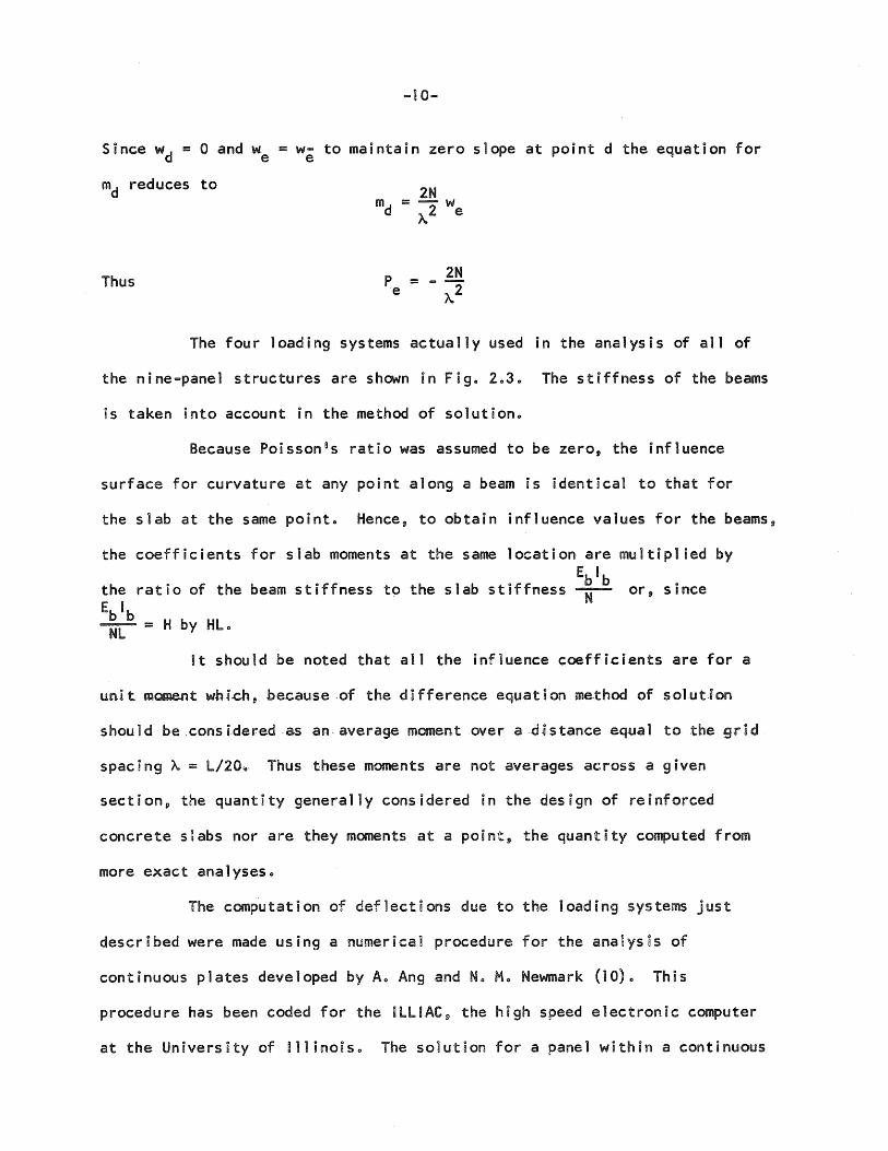
Since wd = 0 and we
md reduces to
Thus
.... 10 ...
= w- to maintain zero slope at point d the equation for e
The four loading systems actually used in the analysis of all of
the nine-panel structures are shown in Figo 2030 The stiffness of the beams
is taken into account in the method of solutiono
Because Poisson 8s ratio was assumed to be zero, the influence
surface for curvature at any point along a beam is identical to that for
the slab at the same pointe Hence, to obtain influence values for the beams p
the coefficients for slab moments at the same location- are multiplied by Eb1b
the ratio of the beam stiffness to the slab stiffness ~ or p since Eb1b 'N'L" = H by Hl"
It should be noted that a11 the influence coefficients are for a
unlt ma:Dent whl.ch, because ,of the difference equateon me.thed of solution
should be.considered ·as an average moment over ad~stance equal to tbe grid
spac i n9 'A. = l/20~· Thus these moments are not averages across a given
section, the quantity generally considered in the design of reinforced
concrete slabs nor are they moments at a po~nt9 the quantity computed from
more exact analyses"
The computation of deflections due to the loading systems just
described were made using a numerical procedure for the analysis of
continuous plates developed by Ao Ang and No Me Newmark (10)" This
procedure has been coded for the ~ll1AC9 the high speed electronic computer
at the University of ~l]inois" The solution for a panel within a continuous
-]1 -=
structure is obtained by superposit~on of single-panel solutionso The
single-panel solutions are determined us~ng finite difference equations and
are therefore not exacto However!) with the aid of a high speed electronic
computer 9 fine grids can be used to obtain the single-panel solutions with
good accuracYg and the numerical procedure used gives solutions for multi-
panel plates with accuracy comparable to that of the corresponding sing1e-
panel solutions.
The solution is divided unto two stepso The first step is to
determine the deflections, moments g and reactions for a single-panel d.ue to
arbitrary boundary conditions!) in this case fixed edgeso The second step
is to compute the deflections of the panel due to changes in rotations and
deflections at the boundary resulting from continuity with adjoining panels,
and superimpose them on the deflections for the fixed edge conditione These
computations are made using an extens~on of Ho Crossos moment dostrobution
procedureo The detans of the distribution procedure are funy described
in Refso (9) and (10)0
203 Results of Computations
Table 201 summarizes and 10cates all of the influence surfaces
obtained in this investigationo The results are presented in two forms;
the influence coefficients are tabulated 8n Figso Aol through Ao 15 In the
Appendix, and the contour maps of the snf]uence surfaces are presented in
Figso 205 through 20190
The fifteen cases considered are grouped according to the four
moment locations designated ]p 2p 3!) and 4 on Figo 2010 The moments at
these locatLons act perpendicular to the section indacated in the figure and I
they are referred to in the text by the following titles~
-12-
Location Positive Moment in Middle Strip
Location 2 ... Negative Moment in Middle Str ip
Location 3 ... Positive Moment in Col umn Str i p
Locat ion 4 ... Negative Moment in Column Strip
The influence surfaces in Figso 2.5 to 20 19 are constructed from a
base plane by laying off ordinates proportional in value at every point to
the particular influence caused by a unit load at the point. The resulting
surfaces can then be represented graphically by a contour map p on which each
contour connects all points of equal influenceo A cross-section of an"
influence surface is an influence line for loads on a particular line of
the structureo
The following convention was used in drawing the influence
~faceso Positive values are shown by solid 1 fnes and negative values by
broken lineso The negative values indicate a reversal in sign of the moment
from the one caused by all panels unif9rmly 1 oaded 0
While influence surfaces give a good overall picture of the effects
of concentrated loads on the slab p they are not particularly useful for
computing the effects of loads distributed over some areao For this
purpose the influence coefficients given in the Appendix are much more
eas i ly usedo
As an example of the use of the influence coefficients in computing
moments p consider the partially loaded area withaM one grid shown in Figo 204.
The moment due to the load is computed by summing up the product of the
corner reactions and the corresponding influence coeff~cients for the node
points of each grido It can be shown that for a unnformly distributed 10ad p
the corner reactions are proportional to the ratio of the rectangular area
formed by 1 ines through the centroid of the loaded area and parallel to the
... 13 ""
grid) ine1) diagonal1.y.opposite the corner!) to the entnre grid areao This
canputation is i l.lustrated in Fogo 2040
204 Discussion of ~nfluence Surfaces
In this section the characteristics of the four groups of influence
surfaces for slab moments and the effect of Hand J on these characteristics
are discussedo The four groups consist of the influence surfaces for slab
moment at locations 1!) 29 3!) and 4 of Fogo 2010 As pointed out previouslY9
the influence surfaces for locations 3 and 4 serve for beam moments as well
as slab momentso
Location 1 - Positive Moment in Middle Strfip
influence surfaces are given in Figso 205!) 206 g and 207 for
positive moment at the middle of the slab for values of H = J = Of) 0025 p
and 00 respecteve1yo The most prominent feature of these surfaces is the
very hi.gh peak.-i3t the location of the momento The surface drops off rapidly
from this point!) the steepest gradfient beong in the dnrection parallel to the
moment 0 (The high peak and the steep gradaent can be seen more easily in
Figo 2020 which contains a sect non taken through the onfiuence surface for
H = J = 00 along a line perpendicu1ar to the section on which the moment
acts and through the point for which the surface is drawn)o There are
negative influence values in the center region of the column strip which runs
perpendicular to the momento The negative values indacate that negative
rather than positive moment as produced at the center of the slab when loads
are placed in this regiono
As the beam stiffnesses Hand J decrease from infinity to zero 9 the
magnitude of the influence coeffIcients ijncreaseso The maxomum positove value
-14-
increases from 00277 to 00302 and the largest negat ive va.1ue increases from
-000016 to .... 0001310 In addition" the shape of the influence sur!aces changes
sl ightlyas .the beam stiffnesses decreaseo The extent of the region in which
there are negative influence coefficients increas~s in a direction perpen
dicular to the moment" and the positive portion of the surface spreads
laterallyo
location 2 ~ Negative Moment in Middle Strip
Influence surfaces are given in Figso 208 0 209" and 2010 for
negative moment at the mid-point of the line connecting the centers of the
columns for H = J = 0, 00251/ and 00 9 respectivelyo: Each of these surfaces
has a gentle slope over most of the panel area except in the region surround
ing the point for which the surface is drawno In thus region the surfac.e _
drops off quite rapidly. This steep drop and the gently sloping region· are
seen more readily in Fig~ 2020 whoch contains a section taken through the
influence surface for H = J = 00 along aline perpendicular to the section
on which the moment acts and through the point for which the surface is
drawn.
As the beam stiffnesses Hand J decre~se from infinity to zero o the
magnitude of the positive influence coefficients decreaseo The maximum
positive value decreases ·from 00285 to 0004430 ~n addition!) a region of
negative influence develops and spreads out around the point for which the
surface is constructed as Hand J decrease from infinityo The infiuence
value at the center of this regGon decreases from zero for H = J = 00 to
the relatively large value of - 00245 for H = J = 00 The development of this
region is accompanied by.a lateral spreading of the contour lones and a
shifting of the point of maxomum posntive value toward the center of the panel.
... 15-
LocatioD_3 - Positive. Moment in Column Strip
I nf 1 uence surf aces are g 8 ven in F i gso 20 11 p 2" 12 j) and 20 13 for
positive moment in the slab at the mid-point of the line joining the centers
of the columns for H = J = Op 0,,25 and 100, respectiveiy" These surfaces
are similar to the ones for positive moment at location 10 They have a sharp
peak at the point for which the surface is drawn" The surface drops off
rapidly from this point and the steepest slope is in the direction parallel
to the mament~, (The high peak and the steep gradient can be seen more easily
in Figo 2021 which contains a section taken through the influence surface for
H = J = 0 along a line perpendicular to the section on which the moment acts
and through the point for which the surface is drawno This section is
almost identical to the one for positive moment at the center of the panel).
There are no negative regions on this surface indicating no reversal in sign
of the moment"
As the beam stiffnesses Hand J decr,ease frOm one to zero!) the
magnitudes of the '8nflue'nce coefficients oncreaseo' The Jmaximum value
increases from 00045 to 003130 In ~dd8tion9 the contour lines of the
surface spread out as the beam stiffness decreases but there is no shift in
the location of the maximum valueo
When the slab influence coeffocaents are multiplied by Hl in order
to find beam moment influence coefficients 9 the beam coefficients decrease
with decreasing values of Hand Jo
location 4 - Negative Moment in Column Strip
Influence surfaces are given sn Figso 2014 to 2oi9 for negative
moment at the center of the column face for H = J = OJ) 0025 9 100 9 and 2.5,;
H = 0025!) J = 100; and H = 19 J = 00250 Ail the surfaces for this moment
-16 ...
are quite similaro They all have a gentle slope over .most of the pane:la.rea
except in the region near the. column face where they drop rapidly.to, z.e,roo
(A section through the surface for H = J = 0 along a line perpendicular to
the section on which the moment acts and through the point for which the
surface is drawn is shown in Figo 2.21). All coefficients are positive with
the one exception of a small region of the surface for H = J = 205 in which
the values are sl ightly negativeo
As the beam stiffnesses are decreased, the influence coefficients
for slab moments increaseo The maximum value increases from 0.028 for
H = J = 2.5 to 0.369 for H = J = 00 There is also a sl ight shift of the
position of maximum influence towaid the column face as the beam stiffness
decreases 0 The effect of J can be observed in two cases by comparing Figs.
2015 and 2016 in which H = 0025 and J = 0025 and 1.0, respectively, and
Figso 2017 and 2.18 in which H = 100 and J = 0025 and 100 respectively.
Such cDmparisons indicate that J has a neg1 ugib]e effect on the maximum
influence coefficient but causes the contour lines to spread out as J
decreases 0
When the slab influence coefficients are multiplied by Hl in order
to find beam moment influence coefficients p the beam coefficients decrease
with decreasing values of Hand Jo
205 Accuracy of Results
Two checks were made on the accuracy of the computer solutionso
One check was to compare the results obtanned herein using finite difference
equations with those obtained by Pucher (2) using a more exact method of
solution. This comparison was made for the posituve moment at midspan and
the negative moment at the middle of an edge for a square plate having
... 17""
clamped edges 0 In Figo 2020 are plotted sections taken through the two
influence surfaces along a line perpendicular to the sections on which the
moments act and through the points for whnch the surfaces are drawno
There is no significant differe~between the influence lines for
positive moment at the center of the plate obtained by the two methods except
at the center pointo Here the exact solution yields a value of infinity
while the finite difference 'solut~on gives a value of 002770
Westergaard (11) studoed the moment directly under a small
circularly loaded area of diameter do He developed an equation for a new
diameter d1 which9 when u~ed with ordinary slab theory and a linear
distribution of flexural stress g gives the same tensile stress in the
bottom of the slab as the theory of thick slabso Although there is some
question regarding the use of such a procedure for computing stresses in
the reinforcement of a concrete slab g it 85 conven~ent9 and the precedent
for its use is well establ ishedo His equatoon for d1 when substituted
into equations for moment at the center of a s~mply supported square slab
results in Eqo 205 which9 however p is approxomate and is based on Poissonos
ratio equal to 00150
where:
p m = -"""';"'--d "" 0 0 049P
o 2032 + 8 "[
m = unit moment directly under a concentrated load o
(2 0 5)
P = concentrated load distr~buted over a circular area of
diameter d
L = span of slab
Vo Po Jensen (5) in his analysis of skew s1abs by finite difference
equations, used Eqo 205 to compute the diameter of a circularly loaded area
which corresponded to his grid spacingo He did this by equating the numerical
... 18 ...
value of the moment directly under a single load computed from finite
difference equations to the moment m given by Eqo 2 0 5 0 - Three grid spacings o
were used in his analysis and the results of the computations gave the
follow.ing values for do
For A. = L/4!) d = 00183L
For A. = L/6!) d = 00123l
For A. = L/10, d = 0.066l
These data were extended in this investigation to include a grid
spacing of A. = L/20 and a corresponding d value of OoOlSl was computed
Figure 2.22 was prepared to summarize all of these results. In the
figure the sol id line represents a section cut through the influence surface
for positive moment at the center of a simply supported square panel as
computed by the theory of medium thsck plates for ~ = 00150 This curve
approaches infinity as X/l approaches zeroo The four dotted curves are
approximate and are drawn to indicate that a transition takes place from the
influence l"ine computed by finite di.fference equations to the one computed
by the theory of medium thuck plateso Thus!) on the'basis of this analysis!)
the influence surfaces developed in this investigation which are based on
A. = L/20 are correct for loads distributed over a relatively sma11 area!)
perhaps as sma] i as, one having a diameter of O.OISLo
A comparison of the two influence 1 ines for negative moments in
Figo 2.21 shows differences of two kindso First 9 in the region near the
boundary!> Pucheros solution gives a 1 imiting influence coefficient of 1/~p
whereas the finite difference equations yield results which decrease to zero
beginning at a distance of about Ooll from the boundaryo ot should be pointed
outl) however, that while the Blexact" solution approaches i/~ at the fixed
edge, it has a discontinuity there since it too drops to zero when the unit
load is directl'y over the f~xed edgeo ~n effec..t.p the. finite differ.eACe
equations round off the discontnnuous OiexactUi curveo The second difference.
in the two curves is that all the finite difference vaiues fan belON the
lIexactBl solutiono There are two reasons for thiso First!) the presence of
columns at the corners of the panel in the finute dnfference solution
reduces the span and thus decreases the momento And secondp the finite
difference solution is for the average moment over a wadth of ~ = l/20
while the' liexactll solution is for the unit moment at a poi~to
The second check involved a compar1son of moments in the nine-panel
stru~ture caused by a unaformly distributed load over a strip of three
adj acent pane 1 s 0 Moments obta B ned by summ i ng the i nf 1 uence .. coeff i c ients.
were compared with moments compu tedd i rec t 1 y.--b.yG 0 Do Hor rison (12) ..us.. i og..
the numerica1 procedure whach is the basis for this investigationo .Table.2~2.
summarizes these comparisonso Atl of the vaiues dbtauned by Morrison were
for a uniform load on the three paneis fin the midd~e row of the nine~panel
structureo This same loading was used an the study for positive moment In
the middle strip ... However!) for the other moments on T.able 202 only the. two
panels contributing the gr.eatest HnfUuence were loadedo Thas accounts for
the small differences observed 0
... 20-
30 MOMENTS DUE TO CONCENTRATED LOADS
301 Concept of an Eguiva1ent Load
In many design procedures slab moments due to concentrated loads
or loads distributed over a part of the panel area are usually computed
using equivalent loads distributed uniformly over the entire panel area.
The accuracy of this procedure depends on the method used to convert the
concentrated load into an equivalent panel loado In this chapter a study is
made of the variables which influence the equivalent panel load to determine
those which are most significanto
The concept of an equivalent load will be developed and discussed
first for the simple case of a beam as an introduction to the more
camp] icated case of a slabo Consider the fixed-end beam shown in Figo 3010
The resultant of the distributed load of length kl is Wand acts a distance
~ from the right endo For the case of k = 0 9 the loading consists of a
sing 1 e concent·ra-ted load and for O· < k < 1 the load i ng cons i s ts of. a
uniformly distributed load over p'art of the span'o The moment Me at the left
end of the beam due to the load W distributed over a length kl is:
[ 2 3 2 JWL
2 Me = 12(a/l) - 12(a/l) + k (1 - 3a/l) -rz- (301)
For an equivalent load CW distributed over the entire length of ,the beam p
the momen tis C W L
12
and for this case 9 the equivalent load factor is~
(3.2)
(303 )
...,21-
This expression shows that C is a function of the posotoon of the load p all
and the proportion of the span length v ko lhe curves on Figo 301 are p10ts
of C vs k for various values of a/Lo Each curve os terminated when the
load extend.s to either the left or right supporto As the load extends over
a greater length of the span (as k sncreases) the curves drop for C greater
than one and ruse for C ]ess than one 0 ~n the specaal case of all = 1/3
there is no variation of C woth ko lhos 65 due to the fact that the
influence 1 ine is anti ... symmetrocal about the poont at all = 1/30 The fact
that the largest values of C are found for all = 2/3 ~ndicates that the
influence 1 nne has a maximum ordinate at all = 2/30
~n the deve10pment of equivalent loads for slabs p a ~im61ar
approach has been usedoHowever v for a slab both the iocation of the
centroid of the loaded area and fits extent can be varned gn two dimensionso
302 Method of Analysis of ~nfluence Surfaces
The method used to study the moments In continuous floor slabs
caused by concentrated loads or ~oads dostrobuted over a part of a panel area
was to compute the moment due to var~ous types of loads placed at nine
different points wothin the pane! areao Sonce at is desBrable to have the
results of this study an a form usefu8 to the desogner using current design
procedures p the concept of an equDva1ent load o somolar to that described
in Section 301 for a beam D was used for the slab and beam moments in the
structures ana1yzedo
The -location of the nine ponnts used on thus study are shown in
Figo 3020 Points were chosen wnthnn on~y one quarter of the panel because of
symmetryo Usang these nine points fit is possible to study the var~ation of
the moments and the corresponding equgvalent ioad factors as loads are moved
about the panei areao
-22-
The loadings considered to act at each of the nine points were a
concentrated load, symmetrical line loads running parallel to the edges of
the panel, and symmetrical rectangular loads extending up to one-third of
the span in each directiono The method of defining the loaded area is shown
in Figo 302 "The length in the x-direction is denoted k l and that in the x
y-direction k Lo ~n each case the length k L or k l is centered on the point y x y
consideredo For k = k = 0 the influence coefficient at the point in x y
question yields the moment for a concentrated load, except when the load is
placed directly over the poont for which the moment is computedo The size of
the loaded area for this case was discussed an Section 2050 When either k x
or k equals zero and the other factor is greater than zero, the loading is y
equivalent to aline 10ado For values of k and k both greater than zero, x y
the shape of the loaded area is square or rectangularo
Moments were computed usnng the procedure outlined in Section 204.
In order to simpl ify the ca]culations 9 the extent of the loaded area was
made to correspond with even multoples of the grad spacingo
The calculation of the equIvalent 10ad factor C was made by
equating the unit moment caused hy a load distributed a.v.e..rpart -of the panel
area to the corresponding unat moment caused b.y--loading- all nine. paneLs
uniformly. The moments used for the case of all panels loaded were taken
from the work of Morrison (12)9 and are 1isted ijn Table 3010 Comparing the
moments caused by loads distributed over a part of the panel area to the
moments caused by all panels loaded as entirely proper for the flat p1ate
since this type of floor system is commonly desugned for uniform load over
all panelso However 9 this is not the case for the two-way slab which is
designed for varoous combinations of panel loadings producing the maximum
possible moment at a given sectiono These moments are greater than the ones
... 23-
for all panels 1 oaded 0 But p since C is computed from the ratio of the
moment for the concentrated load to the moment for all panels loaded, it is
conservative for two-way slabso
An example of the computation of the equBvalent load factor for
negative moment in the column strip (location 4) and H = J = OD caused by a
concentrated load (kx = ky = 0)9 at point A fo11owso The following
notation is used:
m = unit moment produced by a concentrated load
mB = unit moment produced by loading all nine panels
W = concentrated load
C = equivalent load factor p such that a load of CW appl led
uniform1y over each panel will produce the moment mo
From Figo Aol0 in the Appendix9 the influence coefficient at point A
for negative moment in the column strip is 003690 Therefore
m = 00369 W
From Table 3019 the moment coefficient for this same moment location caused
by all panels loaded is 001420 Therefore
m 0 = 00 142 CW
In other words the moment produced at location 4 by a 10ad of
2.60 'W distributed uniformly over each of the nine panels will be equal to
that produced by the concentrated load W at point Ao
Values of C were computed in this manner for k and k ranging from x y
zero to 0035 at each of the nine points and studied to determine the variation
of C with k or k 9 the location of the load in the panel 9 the various values x y
-24-
of Hand J p and the four locations of momento The manner of presenting these
results is described in the next sectoon and the results themse1ves are
discussed in Sections 3049 305 p and 3060
303 Manner of Presentation of Results
The curves in Fogso 303 through 3050 show the variation of the
equivalent load factor C wnth the type of moment D the point at which the
load is placed, and the extent of the loaded area p for the two basic types of
floor systems studiedo The figures are grouped according to the four moment
locations shown in Figo 2010 For each moment location D three sets of curves
are drawn: those that show the varaation ofC with both k and k; those x y
that show the variation of C with k equal to k; and those that show the x y
variation of C for lone loads in both the x- and y-directions extending
across the entire panelo Table 302 summarIzes and locates all of these
curveso
~n constructing these figures the same sign convention was used
as for the influence surfaces; namelYD a reversa~ in sign of the moment or
equivalent load factor is indicated by a minus s09n and a broken linea A
diagram which shows the relative location of each point studied is shown in
the upper right-hand corner of each fagureo The moment considered is
indicated in the diagram by a short line representing the sectson on which
the moment actso When a load is placed directly over the point for which
the moment is computed the value of C os plotted at k = k = 00015 which x y
corresponds to the diameter of the small circular area computed from
Westergaards equation in Section 2050 Attention is called to the fact that
the vertical scale for C is not the same in al1 figureso
~n the first set of curves referred to in Table 3029 the variation
of C is shown as a function of k and k up to a 1 imit .. of 0035 for selected x y
points within the. panel area ..
.... 25 ...
~n all cases k is plotted along the y
horizontal axis and two or more curves are plotted for k 0 All of the x
va1ues of C computed in this study are not ~ncludedo However p the ones
shown are typical. For example p in Figo 303 the curves for point E indicate
that the largest C for this point found within the limits of this study is
for k = 0 and k = 00350 They also ind~cate that C increases as the load x y
is extended in the y-di.r.ec..ti on bu t decreases as ! tis extended in the
x-d i recti ono For thi s poi nt the curves for k = 00 15 and 0025 are omi tted; x
however 0 they fall in the cross-hatched reg~on between the lines for k = 0 x
and 00350 The curves for point B are shown as a broken 1ane because C is
negative p indicating a reversal in sign of the moment at location! when
loads are placed at point Bo These curves show that C decreases as the
loaded area -is increased in s8ze .. Similarlyo the curves for p.oint.H indicate
that C increases as load is sp read 0 n the x-d tree t ion but de.c..r.e.aseswhen load i
is spread in the y-directiono GeneranYpcurves for poi.nts Ap El)'.JFj) and H
are included in all the figures for the general loadingso in addition p curves
for points B and I are included when the value of C 85 not being computed for
that posnto If the curve is not included, a notation is made in the figure
indIcating where it can be foundo When C 8S computed for a moment location
close to either Cp OJ) or Gp the curve for one of these points is includedo
For example p in Figso 303 through 305 for posotive moment an the muddle strip p
curves for point G are included whereas curves for points C and 0 are noto
~n the second set ·of curves referred to in Table 302p the
variation of C is shown for square loaded areas centered at points Ap Bp Ep
F f H p and ~ 0 These eu rves are taken f rom the p rev O"'OUS ones by choos i n9
values of C for k = k 0 x y
-26-
~n the thitd set of curves referred to in Table 302p the variation
of C is shown for 1 ine loads centered on points A9 F9 and i and extended
in increments across the panel iQ the x-dlrect~on9 and for 1 ine loads
centered on points Hand i and extended in increments across the panel in
the y-directiono The notation ~ indicates a line load centered on point x
and extending in the x-directiono
304 Equivalent Load Factors for Moment in a Flat Plate
The equivalent load factors» C9 for the case of H = J = 0 are
presented and discussed in this sectiono They are divided into groups
according to the four moment locations designated 19 2939 and 4 in
~n the fol1owong paragraphs the varoation of the equivalent load
factor C will be discussed with regard to the effect of the position of the
loaded area with respect to the moment location 9 the effect of extending the
loaded area g the effect of increasing the s8ze of square loaded areas p and
the effect of extending 1 ine ]oads across the panelo
Location 1 - Positive Moment on Midd!e Strip
Curves for the value of C for positive moment in the midd1e strip
discussed togethero The maximum value of C for this moment ~ocation varies
from 1203 at point i (Figo 306) down to -005 at poont B (Figo 303)0 The high
value of C at point ~ is found when the load is placed over the ponnt for
which the moment is computedo By comparung the curves for points Fg Gp and
H with those for i it is seen that the extremely hsgh value of C drops off
considerably as the load moves away from this pointo Comparong curves for
... 27-
points Hand F indicates that thus drop is most rapnd 8n the y-directiono
C is negative but small for pODnts A and Bo
Extending the loaded a rea at point ! 8 n both "the x'" and
y-direciions causes a rapid decrease in C; the most rapid-decrease taking
place in the y-directiono C increases at G as the loaded area is extended
in the y-direction until it includes the high peak at point i 9 and then
decreases as load is extended farther in both directionso At point H, C
increases as load is extended in the x-direction toward point I and decreases
slowly as load "is extended in the y ... directiono The effect of extending the
loaded area at points Eand F ~s to cause a small increase in Co In both
cases C increases as load is extended toward point ~, but for point Ep C
decreases whi1e for pointFp it uncreases as load is extended in the
x-directiono Extending the loaded area at points A and B has a negligible
effect on Co
Extending square" area loads p for which k = k 9 combines the x y i
directional effects just discussedo ~n Figo 307 it is seen that as the loaded
area is spread 8 C decreases rapidly at point ~ but does not change nearly
so much at points Av B9 Ep F and Ho
The curves in Figo 3010 show the variation of C as 1 ine 10ads are
extended across the pane10 These curves continue the trends observed in the
curves for the general loadingso Comparing the two curves for line loads
in the x- and y-directions through point ~ (I and ~ ) gives another - x y
indication of the rapid drop of the influence surface in the y-directiono
A comparison of ~ with F and B and ~ with H shows the decreasing x x x y y
importance of line loads for this moment location as one moves away from
toward the ~olumn 1 ineo
-28 ....
location·2 ... Negative Moment In Middle Strip
Curves for the value of C for negative moment in the column strip
be discussed together 0 The equivalent load factors for this momeht location
vary from high negative values for moment under the load to smal1er positive
values in the middle of the panelo Comparing. the curves for points 8 p Fg
and ~ shows that this variation 8S from large negative values down to zero
and then up to smaller positive ones when moving in the y-direction from
point 80 Comparing curves for H with Ip E with Fg and A with 8 shows that C
decreases in magnitude and maintains the same sign as the load moves in the·
x-direction from the line through 8 0 Fv and ~o
Extending the 10aded area fin both directions at point B (Figo .3013)
causes a rapid decrease in C; the more rapid decrease being in the y-directiono
At point Ag C oncreases as load 8S extended in the x-direction toward the
large negative value at point 8 butdec.r.eases when load is .ext.e.nded in the
y-directiono As load is extended-in both d~rections at point F there is a
moderate decrease in C whereas there ~s on]y a sl ight decrease for points I,
The variation of C as square area loads are spread at poonts Ap
B,I E!) F9 H!) and ~ is shown in Figo 30170 The effect of spreading 8S large
at point 8 p moderate at points A and Fo and neg] ngoble at ~9 Hp and Eo
The variations in C observed in the studies lWm~ted to k y= k = 0035 x Y
are extended for 1 nne loads in Figo 30200 The curves for ~ and ~ indicate x y
that 1 ine loads through the center of the panel have about the same effect
up to a length of 006 of the panei Jengtho At this poont p a 1 ine extended
in the y-direction moves into a region of negative influence and causes a
drop in the curve for ~ 0 Curves Hand F indicate that line loads placed y y x
-29-
off of the center 1 ines or co]umn Ulnes of the panel have a smaller effect
on the negative moment in the m!dd]e strip than loads along the column and
center 1 i nes 0
Location 3 -'Positive Moment In Column Strip
Curves for the value of C for posstfive moment in the column strip
be discussed togethero The highest values of C are found for point 80 As
is true for all points where the moment os computed under the 10ad 9 C
decreases quite rapidly as one moves away from the pointo A comparison of
the cu rves f or po i nts Oil F" and with that for AI) shows that the decrease
is more rapid in the x~direct!on than on the y-dBrect90no Comparing the
curves for points E with those for FD H!) and !v and A with 8 shows the values
of C drop off as one moves In the x-d I rect non from a 1 ineth.r~ .B!) F 9' and i 0
As the loaded area is spread out at point B!) C decreases; the most
rapid decrease takong place fin the x-dorectoono At point 0" C increas.es as
the loaded area is extended on the x-do~ectoon to k = 0025 and then x
decreases as it is extended farther!) and C decreases slightly as the load
is extended in the y-directoono At point F!) C decreases moderately when
the loaded area is extended ~n the x=dsrection but increases only slightly
when the load is extended on the y-dnrectiono There as a small variation of
C for points H and ~ and a ~fitt]e larger varoatBon at points A and Eo
Figure 3027 shows the varnatoon of C for square loaded areas of
various s8zes centered on points AI) Bo Ep F!) Hp and ~o The curves for points
F" 19 E" and A are almost entBrely nndependent of the sIze of the loaded
areao There is a large decrease on C for point B and a small increase for
point A as the loaded area os enlargedo
-30 ...
Fi.gure 3-030 shows the var8ation of C as 1 ine loads are ex.tended
across the panel areao Comparong curves B ~ F 0 and i shows the decrease x x x
in C that takes place as 1 ine loads are moved from the column lineo A
comparison of curves i and H indicates the decrease in C as 1 ine loads are y y
moved away f rom the center of the pane 1 in the x ... d i rect ion 0 F i nail y,
compar B ng curves ~ wi th i i nd i cates the increase 8 n C that t.akes place as x y
load is extended toward the hngh peak at point Bo
location· 4 - Negative Moment in Column Strip
Curves for the value of C for negative moment in the column strip
are presented in Fogso 3033 0 3039 p and 30450 The extremely large factors
found for the other three moment locations do not exist here because the
moment becomes zero when the load is placed at the point for which the
moment is computed 0 The largest values of C are found at point A and they
decrease as one moves away in either the x'" or y .... directions; the largest
decrease takes place on the y-dnrect8ono As the load moves from the corner
of the column along a lone through points Co ED and iD the equivalent load
factor first increases up to pOHnt E where !t reaches a maximum and then
decreases as one continues on to point io ~n genera] 0 the changes ~n C that
take place as one moves from point to point are gradualo
Except for points AD ED and CD the effect of extending the loaded
area is to cause a sl ight reduction in C factorso At point A, C decreases
as 10ad 85 extended en both the x- and y-directoons; the reductions in the
x-direction being slightly ~ess than in the y-directaono At point E9 C
increases sl ightly when load is extended fin the y-direction but decreases
when extended on the x-directiono The equivalent load factors for point C
increase as the loaded area is extended in the y-directions up to k = 0025 9 Y
-31-
after which they decreaseD whereas C increases as load is extended in the
x-d i rect i ono
Figure 3039 shows that C varies only 51 ~ghtly as square loaded
areas are spread at points Sp Ep Fo H9 and ~o There os small reduction in C
when a load at point A is spread over a larger areao
The curves in Fugo 3045 show the varIation of C as ione loads are
extended across the panel 0 A comparison of curves B 9 F p and ~ indicates x x x
the decreasing effect of line loads as they are moved away from the column
1 ineo Curves I and ~ show that C decreases when a j ine load is extended x y
in the x-direction but increases when at as extended on the y-directiono
Curves Hand i show the sma]l effect of 1 ine loads perpendicular to the y y
direction of the moment at the face of the columno
305 Equivalent Load Factors for Slab Moments in a Two-Way Slab
in this section the equivalent load factors C9 for siab moments
in two-way slabs supported on beams having stiffnesses of H = J = 0025 and
00 are presented and discussedo They are divided into two groups according
to the two moment locations designated 1 and 2 in F~go 2010
Location 1 - Positive Moment in Middle Strip
309 p 30 l1v and 30120 for the pos~tive mome~t at the center of the pane10
The general shapes of all these curves are very similar to the corresponding
ones for the flat plate (H = J = 0); however p each band of curves for the
various points sh·ifts up or down as the beam stiffness 8S increasedo By
comparing the curves for points AD Bo Eo Fv and H on Figso 303 through 305 it
is seen that the bands for these points are lowered as the beam stiffness
is increasedo This downward shift indicates a decrease in the equivalent
... 32-
load fa,ctor for these pointso The curves for points A and B are.not.shown
in Figo 305 becaus.e C is extremely small,o The band of curves for point G
first- drops s1 ightly and then rises as the beam stnffness is increased ..
The curves for point I in Figo 306 show that C increases as the beam stiffness
is increased 0
The curves for area loads in Figso 307 p 308 p and 309 fol1ow the same
patterns described for the general 1 oads 0
The curves for 1 ine loads in Figso 30 lao 3011p and 3.12 are similar
in shape to the ones for H = J = 0 but have been shifted up or down slightly.
Curves for B p F 9 and H drop whereas the highest point on the curves for x x y
I x and i y moves upward as the beam s t 8 ffness is i ncreasecL
Figure 3051 summarfizes the variations of C with H for moment location
1 ~n this figure p values of C are plotted versus the para~ter 1 + 4H/3 0
1 A parameter of the form 1 + 'rH was chosen so that values of C rang.ing from
H = 0 to H = 00 could be included conveniently on the same curveo For
an isolated slab supported on flexible beams 9 r = 2 since the resistong
moment acting on a section through the slab includes two beam moments and one
s.1ab moment 0 For the nine-panel structure p r = 4/3 since the resisting
moment in this case consists of four beam moments and three siab momentso
The values of C in th8s figure are the maximum values found within the limits
of this study except for one curve for poant I .corresponding to k = k = 0035 x y
which gives the lowest value of C at point ~o These curves emphasDze the
small variation of C with beam stiffnesso The largest variation in C is for
the moment directly beneath a concentrated ]oad at ponnt ~o ~f this load
is spread out over an area corresponding to k = k = 0035 9 not only does x y
the factor decrease on magnitude but its variation with beam stiffness
... 33-
decreases 0 i ngenera 1 I) the beam stiffness has 1 itt 1 e effect .OA tbe.
equivalent load factor for positive s]ab moment ijn the middle stripo
location 2 - Negative Moment in Middle Strop
Curves for the values of C are given in Figso 30149 3015 9 3016 9
3018S) 30191) 3021S) 3022 for the negative moment at the mid-point of the line
connecting the center of the co1umnso Attentoon is called to the fact that
different scales are used in Fags03.14 and 3016 than in the other figures
for this moment locationo These curves are quote different than the ones. for
the flat plate (H = J = O)~ They indlcate that as the beam stiffness
increases there is a rapid decrease sn the magnitude of the negative values
of C accompanied by n ncreases in the mag.n B tude of the pos it ive va 1 ues 0 ..
Comparison of the curves for the points in Fogo 30 ]6 shows that C decreases
from a large ne.gative value to a smaller posotove value as the beam
stiffness increaseso ~n Fugso 30 ~3 through 30 ~5 a snmolar trend is oos..erved
for point Ao These figures also indncate that v wnth increasong beam stiffness,
C increases at points E and Fv Is aimost constant at point HS) and first
decreases slightly and then increases at poont ~o I • I
These curves also nndncate that the range on C caused by extending
the loaded area is also affected by beam staffnesso As the beam stiffness
increases!) the range in C decreases at ponnts Av Sv and H whereas it increases
at points ED Fg and ~o
The trends observed for the genera] loadong curves are also
observed in the curves for the square ~oaded areas in Figso 3Q17» 3018 and
Comparison of Figso 3020 v 3021D 3022 shows the variation of C for
1 ine loads as they are extended across the slab in the x= and y-dorectionso
-34-
As beam stiffn.ess increases 9 C decreases for B , increases for F , I and x x x
~ 9 and decreases sl ightly and then increases for H 0 In additioo, the y y
shapes. of the curves are chan,geda As beam stiffness increases 9 the curves
for 1 in,e load Bx become flatter, indicating less variation in C as the 1 ine
load is extended across the pane 1; those for F become steeper!) i nd.i.~.at.i.ng x
a greater variation; and those for 1X9 Iy» and Hy undergo minor changes but
remains rather flat.
Figure 3052 11 which has the same format as Figo 3051, summarizes the
variation of C for moment location 20 It emphasizes the fact that beam
stiffness has a large effect on Cg especially for points A and B which are
on the beamo The curves also show a shift of the maximum positive value of
C toward the middle of the panel with increasing beam stiffnesso
306 Eguivalent Load Factors for Moment in Beams Supporting Two-Way Slabs
Curves for the equivalent load factor!) Cil for positive and negative
moments in beams supporting two-way slabs at locations 3 and 4in Figo 201
are presented and discussed in this sectiono Because ~ = 0 was used in the
computations» beam moments are found by multiplying the corresponding slab
moment by HL. Thus!) since Hl is common to both the moment caused by a
concentrated load and the moment caused by a uniformly distributed load over
all nine panels g the ratio of these two moments ll C9 is the same for the
moments in the slab and in the beamo However p since the s1ab moment is small
at locations 3 and 49 the C factors are discussed in terms of beam moments.
Location 3 - Positive Moment in Beams
Equivalent load factors for positive moment at the center of the
-35-
for va·lues'of H =J =Oo25and·l000 'With the exceptiori of the c'urvesfor
point Sp all of these curves are very similar tb the corresponding ones for
H = J = 00 In the case of point Sf) shown in Fig. 3~26p C for k = k = 0 x y
decreases as the beam stiffness increases, whereas it becomes almost constant
with H as the loaded area is extended up to k = k = 0.35. Figure 3053 x y
which is similar to Figs. 3.51 and 3.52 shows the variation of the maximum
value of Co In general the beam stiffness has a small effect on the value
of the equivalent load factor for positive moment in the column stripe
Location 4 - Negative Moment in Column Strip
Equivalent load factors for negative moment at the face of the
3.50 for values of H = J = 0.25, 100 and 205. Additional curves for the
case of H = 0025, J = 1.0 and H = 1.0 9 J = 0.25 are shown in Figso 3035,
3036 p 3.41 p 3042, 3047 g and 3048. All of the curves in these figures are
similar to the corresponding ones for the case of H = J = 00 In the case
of points Ap S, F, and E, C first decreases and then increases as the
beam flexural and torsional stiffness as increased 9 whereas C decreases
continuously at points ~ and H as the beam stiffness is increased.
Comparison of Figs. 3034 and 3.35 indicates an increase in C for points A and
B as the torsional stiffness of the beam 8S increased whereas there os very
1 ittle change in C for the other poijntso However g this trend is not
observed in Figso 3036 and 3.37 in which H = 1 and J is increased from 0.25
to 1.00 The variation of C with H for k = k = 0 is shown on Figo 3054 x y
which has the same format as Fig. 3051. These curves show the small variation
in C as the beam stiffness is increased. The curves for the area loads and
for the line loads follow the same patterns described for the general
loadi.ngs; namely a slight decrease in C up to H =: 0,25 and then an increase
fo,r points A, B, F, and E and a decrease for points I and H as the beam
stiffnesses are increased. i
-37-
4. EXAMPLES OF USE OF LOAD FACTORS
40 1 F 1 at Slab s
(a) Concentrated Loads
In the investigation of a floor system designed for a uniformly
distributed load over all panels 9 the question is how large a concentrated
load can be placed at a given point or at any point within the panel 0 On
the other hand, in the design of a floor system subject to concentrated
loads II the question is what Blequ ivalentDi uniformly distributed load should
be used in the computation of the moments at the critical sectionso In
the following paragraphs answers to these questBons are deve 1 oped 0
On the basis of the curves for load factors in Chapter 3, it is
evident that the effect of extending the loaded area is small except for
moments directly under the ioado The positson of the load within the panel
area is the major factor to be consodered an estab1ishing load factors 9 both
for design and for investigation of flat plateso These general conclusions
will be used to develop simplified onfluence surfaces for load factors for
the flat plate type floor systemo,' The simplified diagrams win then be
used to investigate a typical designo
~n Table 401a p the maximum load factors found within the J imits
of this investigatoon for the case of H = J = 0 are tabulated for various
moment locations and load pos.itions within the panel areao These are
maximum values which represent an upper limit to the ioad factors computed
in thos investigation and neglect the effect of the area over which the
load is spreado Figure 401 was constructed an order to show graphically the
variation of the load factors tabulated in Table 401ao ~n this fijgure 9 the
regions of the slab having comparable values of C are shown for each of
the four moment locationso Only ~ quarter of the panel is considered
... 38-
because of symmetry 0 The ranges shown in the figure were established by
grouping the values in Table 401a for points adjacent to one another and for
points having C values of the same relative magnitude and signo The ranges
in C were made wide enough so that no discontinuities existed at the
boundar i es 0 ~ n some reg ions l> both pos i t lve and negat ive va 1 ues are necessary
because of the reversal in sign of the moment caused by loads at particular
pointso Small circular areas of radius OolL were used where the load factor
appl ies to the moment directly under the loaded areao The radius of o. IL was
chosen since in this instance the effect of distributing the load and the
effect of moving the load from the high peak Oh the influence surface
reduced C appreciablyo The arrows shown in Fogo 401 indicate the direction
in wh~ch C is decreasing thus indicate how to interpolate for intermediate
pointso Final1Y9 in Figo 402{a) the maximum load factors p regardless of
moment location are grouped and regoons established using the same
technique as for Figo 4010
The moments to be used in desagnong a fiat plate for a fixed
concentrated load can be computed using the appropriate load factors from
Figo 4010 For exampleD if a flat plate 20 by 20 ft 6S to be designed for a
concentrated load of 10 kips at point P (x = 003l and y = Oo2l) the
fol1owing Blequ ivalent Oi uniformly d~stributed live loads should be used in
conjunction with existing formulas for uniform 10ads to compute the
moment at the four critical moment 10cationso
Moment locat i on
2
3
4
load Factor
1 05
100
105
1 05
Uniformly Distributed live load» psf
3705
2500
3705
3705
-39 ....
The load factor given in the table above for moment location 1 was
taken as 105 since point P is approximately midway between one region where
C is 100 or -0.5 and another region where C is 200 to 4000 A C factor of 100
for moment location 2 was chosen because point P is well removed from the
point of the right positive load factoro The values for the other two
locations were establ ished in a similar mannero
The moments to be used in the design of a flat plate for a roving
concentrated load which can be placed at any point on the slab are found by
using the highest load factor for each point to compute full pane1 loadso
For example, if a flat plate 20 by 20 ft is. to carry a concentrated load of
10 kips at any point in the panel the following load factors and uniformly
distributed 10ad should be used to compute the critical. moments 0
Moment location
2
3
4
load Factor
12 or -005
-8 or 1 05
6
205
UnBformly Distributed live load p psf
300 or -1205
200* or 3705
150
6205
If the 200 psf marked with an asterisk is equal to or less than
the dead 10ad 9 positive moment reinforcement at iocation 2 is not necessaryo
However p if it is larger than the dead 10ad o positive moment reinforcement
is necessaryo
When investigating a slab v the load factors in Figo 402(a} shou1d
be consideredo The permissible concentrated load which can be placed at, a
given location is found by dividing the total panel load by the appropriate
load factoro On the basis of the 10ad factors in Figo 402(a}9 the allowable
concentrated load within the five regions for a slab 20 by 20 ft desogned
to carry 200 psf 1 ive load and 100 psf dead load are
-40-
Region Load Factor Load n Kips
I 12.0 607
II -8.0 or 6 .. 0 5* or 1303
III 105 to 400 5303 to 20
IV 1 ,,5 to 2 5303 to 40
V -105 or 2 to 205 6607* or 40 to 32
The load shown above for Region I is computed by dividing the total
panel 1 ive 10ad of 80 kips (20 x 20 x 002) by the load factor 120 The
positive value for Region i I is found by dividing the total 1 ive load by 6
and the negative value is found by dividing the total dead load of 40 kips
by the load factor 8000 The loads marked with an asterisk are permissible
loads if special reinforcing steel is not provided" That is, loads in
these regions cause a reversal on sign of moment at one of the four moment
locations and thus require reinforcement on the opposite face of the s1ab
from where it is normally placedo The loads marked with the asterisk are
chosen so that the moment produced by the dead load is equal to the moment
of opposite sign produced by the concentrated load" The load which can be
placed at any point on the slab is the smallest of these values; namely
5 kips ..
(b) Loads Distributed Over a Small Area
A common specification of many building codes is that the floor
system be proportioned to carry a load of 29000 lb distributed over a
2;S-ft square area and placed so as to produce maximum moments 0 Equivalent
uniform loads satisfying this specefication are tabuiated in Table 402 for
three panel slzeso ~n computing these values p account has been taken of
the effect of spreading the load over the 2o?-ft square areao ~f the
negative loads for location 2 are greater than the dead 10ad p positive
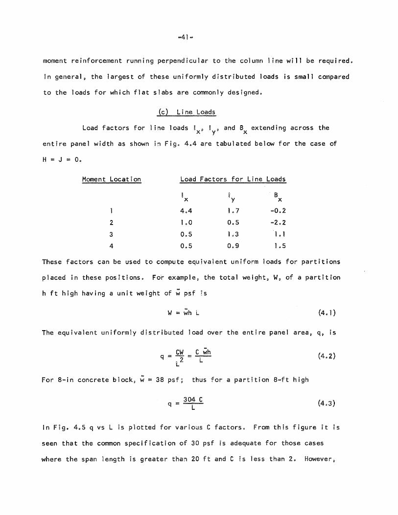
-41-
moment reinforcement running perpendicular to the column 1 ine will be requiredo
~n general p the largest of these uniformly distributed loads is small compared
to the loads for which flat slabs are commonly designedo
(c) Line Loads
Load factors for 1 ine loads I D ! 9 and B extending across the x y x
entire panel width as shown ~n Figo 404 are tabulated below for the case of
H = J = 00
Moment Location
2
3
4
Load
I x
404
1 00
005
005
Factors for Line Loads
~ B Y x
1 0 7 ... 002
005 ... 202
1 .; 3 I 0 1
009 I 05
These factors can be used to compute equivalent uniform loads for partitions
placed in these positionso Fo~ exampleD the total weight 9 Wp of a partition
h ft high having a unit weight of w psf is
W = wh L
The equiva1ent uniformly distributed load over the entire panel area p qp is
CW C wh q=l2=-L-
For 8-in concrete block p w = 38 psf; thus for a partition 8-ft high
q = 304 C L
In Figo 405 q vs l is plotted for various C factorso From this figure it is
seen that the common specification of 30 psf 85 adequate for those cases
where the span length is greater than 20 ft and C is less than 20 However p
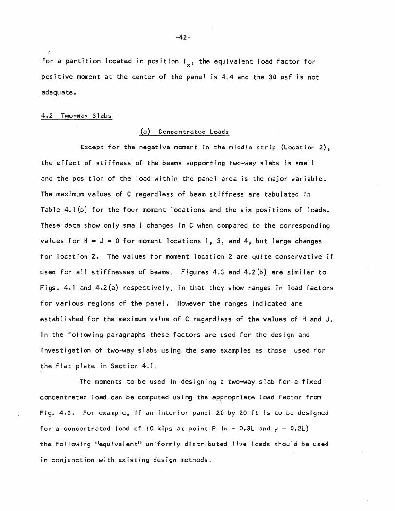
-42-
(
for a partition located in position I 9 the equivalent load factor for x
positive moment at the center of the panel is 404 and the 30 psf is not
adequateo
402 Two-Way Slabs
(a) Concentrated Loads
Except for the negative moment in the middle strip (Location 2)9
the effect of stiffness of the beams supporting two-way slabs is small
and the position of the load within the pane) area is the major variableo
The maximum values of C regard Jess of beam stiffness are tabulated in
Table 401 (b) for the four moment locations and the six positions of loadso
These data show only small changes in C when compared to the corresponding
values for H = J = 0 for moment locations 19 3 9 and 49 but Jarge changes
for location 20 The values for moment location 2 are quite conservative if
used for al1 stiffnesses of beamso Figures 403 and 402(b) are ssmilar to
Figso 401 and 402{a) respectivelY9 in that they show ranges in load factors
for vari.ous regions of the panel 0 However the ranges indicated are
established for the maximum value of C regardless of the va1ues of Hand Jo
in the following paragraphs these factors are used for the design and
investigation of two-way slabs using the same examples as those used for
the flat plate in Section 4010
The moments to be used in designing a two-way slab for a fixed
concentrated load can be computed using the appropriate load factor fram
Figo 4030 For example 9 if an interior panel 20 by 20 ft 5S to be designed
for a concentrated load of 10 kips at point P (x = Oo3l and y = 002l)
the following liequ ivalent Bi uniformly distrobuted 1 ive loads should be used
in conjunction with existing design methodso
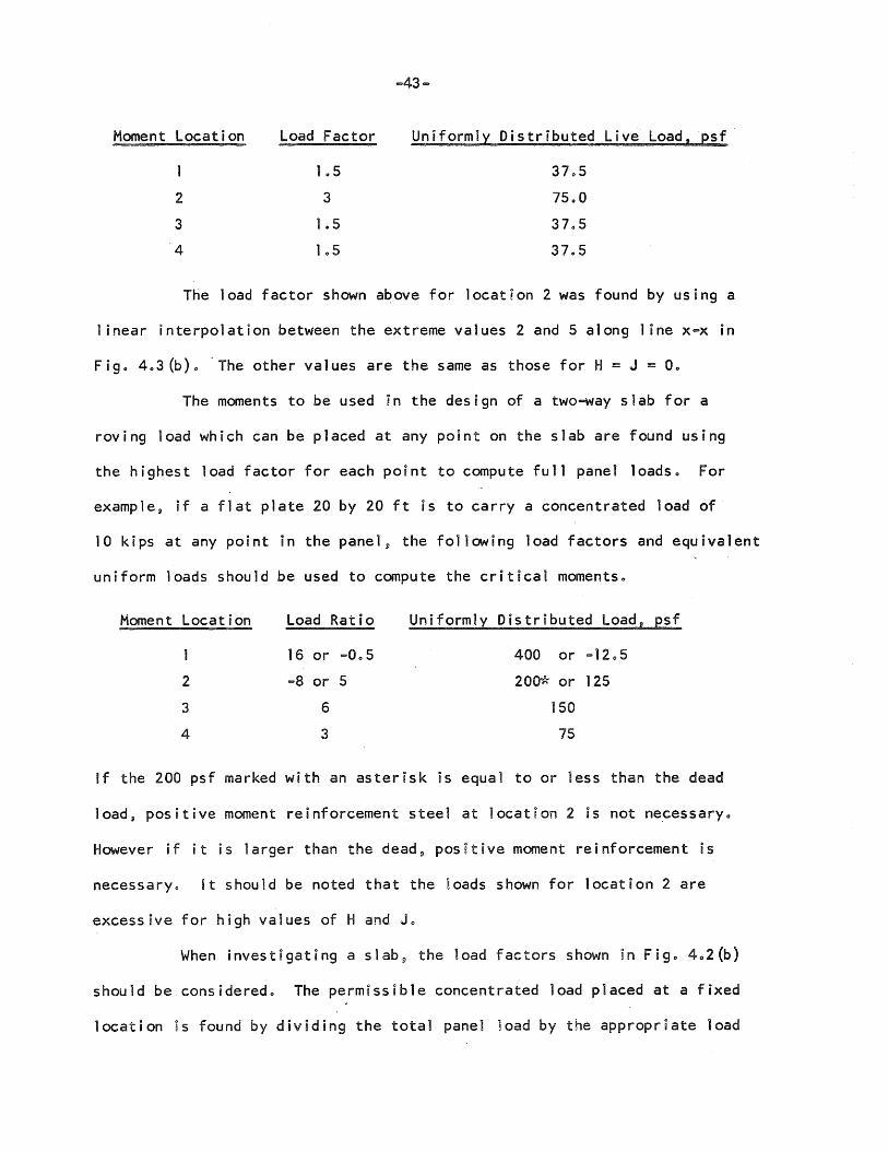
Moment Location
2
3
4
... 43-
Load Factor Uniformly
1 05
3
1 05
1 ,,5
Distributed Live Load, psf
3705
75 .. 0
37" 5
37" 5
The load factor shown above for location 2 was found by using a
1 inear interpolation between the extreme values 2 and 5 along 1 ine x-x in
Figo 403 (b)" -The other values are the same as those for H = J = 00
The moments to be used in the design of a two-way slab for a
roving load which can be placed at any point on the slab are found using
the highest load factor for each point to compute full panel loadso For
example p if a flat plate 20 by 20 ft is to carry a concentrated load of
10 kips at any point in the panel p the following load factors and equivalent
uniform loads should be used to compute the critical moments 0
Moment Location
2
3
4
Load Ratio
16 or -005
... 8 or 5
6
3
Uniformly Distributed Load" psf
400 or ... 1205
200"k or 125
~50
75
If the 200 psf marked with an asterisk is equal to or less than the dead
10ad s positive moment reinforcement steel at location 2 is not necessary ..
However if it is larger than the dead, positive moment reinforcement is
necessaryo it should be noted that the loads shown for location 2 are
excessive for high values of Hand Jo
When investigating a slab p the load factors shown in Figo 402(b)
should be consideredo The permissible concentrated ]oad placed at a fixed
location is found by div!ding the total panel load by the appropriate load
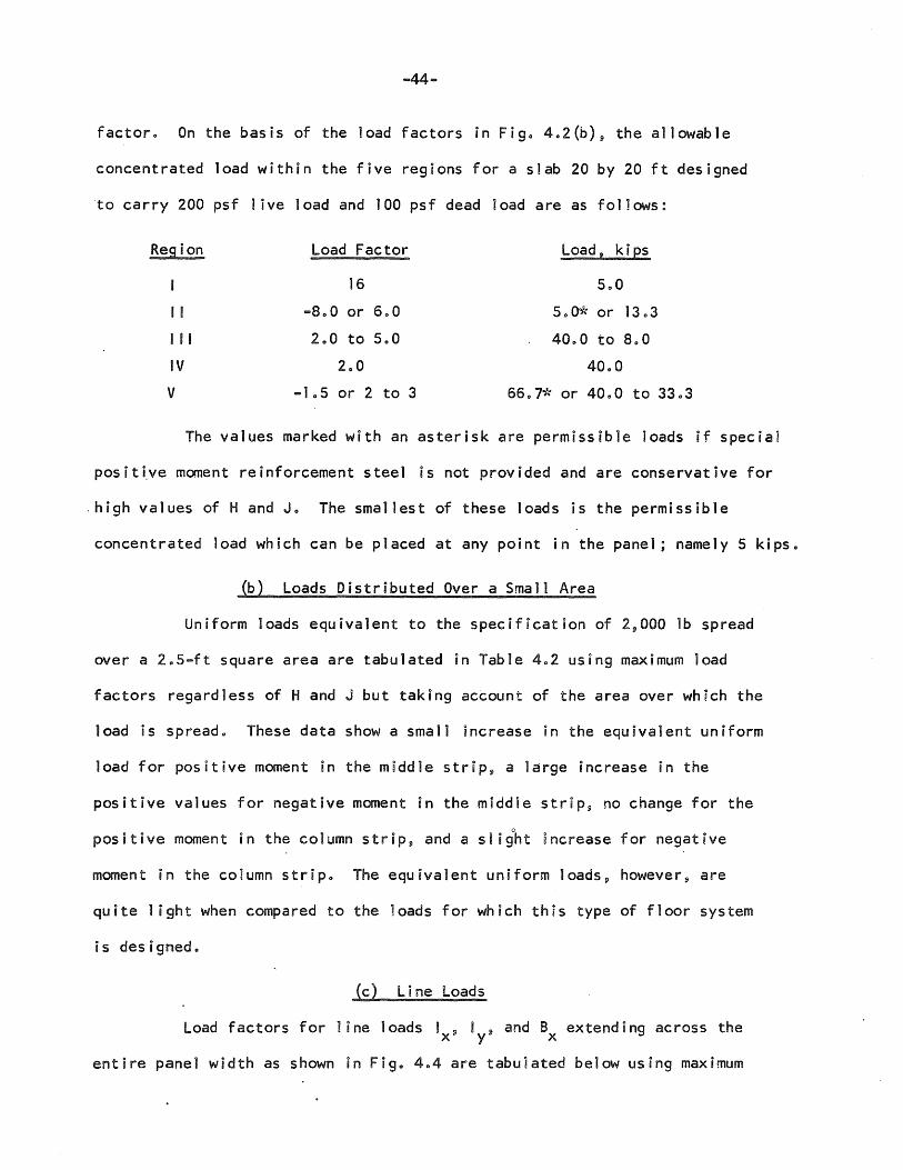
-44-
factoro On the basis of the load factors in Figo 4.2(b)9 the allowable
concentrated load within the five regions for a s1ab 20 by 20 ft designed
to carry 200 psf 1 ive load and 100 psf dead load are as follows:
Region
II
III
IV
V
Load Factor
16
-800 or 600
200 to 500
200
-105 or 2 to 3
Load, kips
500
500* or 1303
40~0 to 800
4000
6607* or 4000 to 3303
The values marked with an asterisk are permissible loads if special
positi.ve moment reinforcement steel is not provided and are conservative for
. high values of Hand Jo The smallest of these loads is the permissible
concentrated load which can be placed at any point in the panel; namely 5 kipso
(b) Loads Distributed Over a Small Area
Uniform loads equivalent to the specification of 2,000 lb spread
over a 205-ft square area are tabulated in Table 402 using maximum load
factors regardless of Hand J but taking account of the area over which the
load is spreado These data show a sma11 increase in the equivalent uniform
load for positive moment in the middle strip~ a large increase in the
positive values for negative moment in the middie strips no change for the
positive moment in the column strip9 and a slight increase for negative
moment in the column stripo The equivalent uniform loads p however 9 are
quite 1 ight when compared to the loads for which this type of floor system
is designed.
(c) line loads
Load factors for line loads I 9 I 9 and B extending across the x y x
entire pane] width as shown in Figo 404 are tabulated below using maximum
-45-
values regardless of Hand J.
Moment location load Factors for line loads
I I B x Y x
4.4 109 -002
2 1 03 205 -202
3 006 1 03 103
4 005 1 00 100
These values, when used in conjunction with Fig. 405, which applies to the
case of an 8-in. concrete block partition 8-ft high g can be used to find
equivalent uniformly distributed panel loads for design purposes. These
results indicate the same general conclusion reached for flat slabso -<
403 limitations of Numerical Results
Because of the geometry of the structure analyzed, the limited scope
of the analysis, and the assumption made in estab1 ushing the loads in these
examples» the numerical results presented above are illustrative rather
than general 0 A summary of the assumption made os given belowo
10 The structure analyzed is the interior p~nel of nine square
panels arranged three by three and having uniform slab thickness and in-
finitely stiff columns which have a ell ratio of 0010
2. The computations of the influence coefficients are based on ~.
elastic behavior of the slab and beams with PoissonBs ratio equal to zero
and are made using a numerical procedure based on finite ~ifference equationso
3. The equivalent load factors for area loads are computed for an
area extending up to one-third of the span length in each direction, thus
1 imiting the size of the loaded area to about iO per cent of the panel areao
The load factors used to compute the loads in the examples of this chapter
are based on maximum values and hence are usually conservativeo However~
i
-46-
using complicated relationships rather than maximum values is not
justified because of the I imitations of geometry of the structure and the
assumptions made in the analysiso
-47-
50 SUMMARY AND GENERAL CONCLUSiONS
50 1 Ou t 1 i ne of I nves t i ga t i on
The analytical study presented in this report is concerned w~th
the moments in continuous floor slabs produced by concentrated loadso
Influence coefficients were computed for four moment locations
in the interior panel of a continuous structure composed of nine square
panels arranged three by three and supported along the edges by flexible
beams (Fig. 201)0 If the supporting beams have zero flexural and torsional
stiffnesses, the nine-panel structure is representative of the type of floor
system known as the flat plate; when the beams are considered to have
stiffness 9 the structure analyzed is similar to the type of f100r system
called a two-way slabo Slab moments were obtained for values ofH and J
ranging from zero to infinitY9 and beam moments were obtained for values
of Hand J of 0025, 100 8 and 2050
The computation of the influence coefficients for the structure
was made using a numeri~al procedure whoch was coded for the ~LLiAC9 one of
the digital computers at the University of nlinoiso This procedure j·nvoives
the use of finite differences and is duvided into two stepse in the first
step9 the deflections 9 momentsj) and shears for a single panel with fixed-.edge
boundary conditions are computed. in the second step9 the deflections at
the boundary resulting from continuity with adjoining panels are computed
and superimposed on the defiectnons for the fixed-edge conditione The
loading systems shown in Figso 202 and 2.3 were used in the computations.
These loading systems were determined using a procedure described by No Mo
Newmarko Since a fine network of 400 squares was used in writing the
finite difference .equat ions !) the approxumate solution was found to be quite
accurate when compared with BiexactOO so] uti ons.
-48-
The influence coefficients obtained for the four moment locations
common1y considered in the design of continuous floor systems have been
presented graphically by mea~s of influence surfaces which are similar to
inf1uence 1 ines for beams. A study was made of the influence surfaces to
determine the significant variables ;by computing moments for concentrated
loads, area loads extending one-third of the span length in each direction,
or line loads running across the entire panel width and parallel to the
panel boundaries. The resu1ts have been interpreted and made suitable for
practical use by introducing the concept of an equivalent panel load, which
when distributed uniformly over the entire pane] and used with conventional
design procedures, gives an effect equal to that of the load distributed
over a small area o
The equivalent panel load is computed by mu1tiplying the con
centrated load by an equivalent load factor Co These equivalent load factors
are plotted for the four moment 10cations 9 for various loadings, and for
various flexural and torsional stiffnesses of the beamso
Several examples of the appl Bcation of load factors in problems
of both'design and investigation are goven in Chapter 4 for both the f1at
plate and the two-way slabo Considerable simplification is made in these
examp1es by using maximum 10ad factors without regard to the area over
which the load is placed or the stiffness of the edge beamso
502 General Conclusions
The following general conclusions from the results of this
investigation are bel ieved to be applicable to al] continuous two-way floor
slabs supported on flexible beams.
The position of the load with respect to the moment location is
the most important variable to be considered in the computation of moments
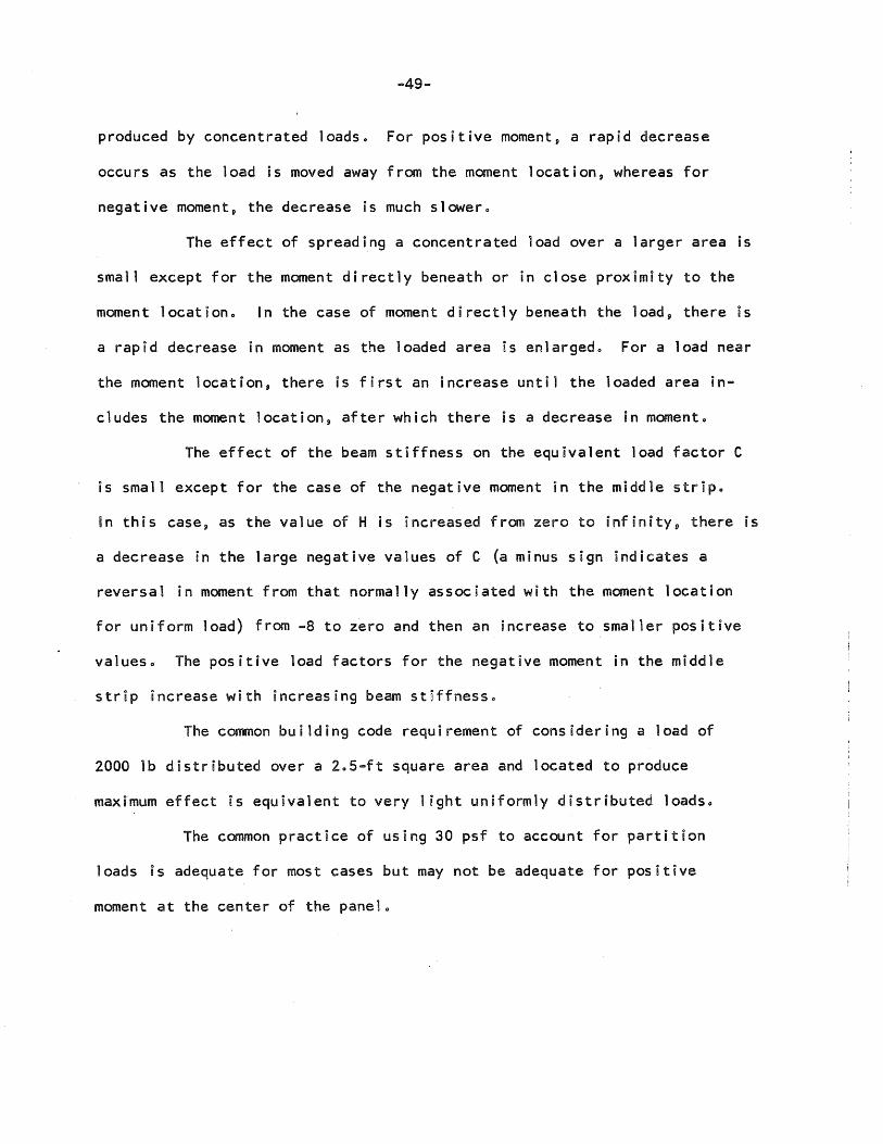
-49-
produced by concentrated loads. For positive moment, a rapid decrease
occurs as the load is moved away from the moment location, whereas for
negative moment p the decrease is much slowero
The effect of spreading a concentrated load over a larger area is
small except for the moment directly beneath or in close proximity to the
moment locationo In the case of moment directly beneath the load p there is
a rapid decrease in moment as the loaded area is enlargedo For a load near
the moment location, there is first an increase until the loaded area in
cludes the moment location, after which there is a decrease in momento
The effect of the beam stiffness on the equivalent load factor C
is small except for the case of the negative moment in the middle strip.
In this case, as the value of H is increased from zero to infinity, there is
a decrease in the large negative values of C (a minus sign indicates a
reversal in moment from that normally associated with the moment location
for uniform load) from -8 to zero and then an increase to smaller positive
valueso The positive load factors for the negative moment in the midd1e
strip increase with increasing beam stijffnesso
The common building code requirement of considering a load of
2000 lb distributed over a 2a5-ft square area and located to produce
maximum effect is equivalent to very 1 ight uniformly distributed 10adso
The cammon practice of using 30 psf to account for partition
loads is adequate for most cases but may not be adequate for positive
moment at the center of the panel 0
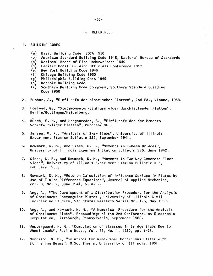
... 50 ...
60 REFERENCES
10 BUILDING CODES
(a) Basic Building Code BOCA 1950 (b) American S~andard Building Code 1945 9 National Bureau of Standards (c) National Board of Fire Underwriters 1949 (d) Pacific Coast Building Officials Conference ]952 (e) New York Building Code 1946 (f) Chicago Building Code 1950 (g) Philadelphia Building Code 1949 (h) Detroit Building Code (i) Southern Building Code Congress, Southern Standard Building
Code 1950
2. Pucher, Ao, DlEinflussfelder elastischer Platten U8, 2nd Edo ll Vienna, 19580
30 Hoeland ll Go, DiStutzmomenten-Einflussfelder durchlaufender Platten8l g Berl in/Gottingen/Heidelbergo
4. RUschl/ Eo Heg and Hergenroder, AOI) DtEinflussfe1der der Momente Schiefwinkliger PlattenUl
p Munchen/19610
5. Jensen p Vo POl) BUAnalysis of Skew Slabs Hl , University.of Illinois Experiment Station Bulletin 332, September 19410
6e Newmark p No Mop and Siessf} Co Pog oBMoments in ~"'Beam Bridges USIl
University of 111 inofs Experiment Station Bulletin 336 9 June 19420
70S i ess, CoP 0 11 and Newmark~ No Mo f} uBMoments in Two-Way Concrete Floor Slabs iB
lJ University of illinois Experiment Station Bulletin 385 9
February 19500
8. Newmarkp No MOl) BONote on Calculation of ~nfluence Surface in Plates by Use of Fin i te Difference Equat i ons oo
!) Jou rna 1 of App 1 i ed Mechan i cs lJ
Vol. 8 p Noo 29 June 1941 p po A-920
90 Angp Ao, '~he Development of a Distribution Procedure for the Analysis of Continuous Rectangular Piates B1
D University of nlinois Civil Engineering Studies» Structural Research Series Noo 176, May 19590
100 Ang, AOf) and Newmark p N. Mop BOA Numerical Procedure for the Ana1ysis of Continuous Slabs 0i
9 Proceedfings of the 2nd Conference on Electronic Computation, Pittsburghf} Pennsylvania p September 19604
110 Westergaard, Ho MOll DiComputation of Stresses in Bridge Slabs Due to Wheel Loads Di
lJ Public Roads D Volo ~~!) Noo ID 1930 9 ppo 1-230
120 Morrison, Go Do, BBS olutions for Nine-Panel Continuous Plates with Stiffening Beams 6i l) MoSco Thesis!) University of ~l!inoisl) 19610
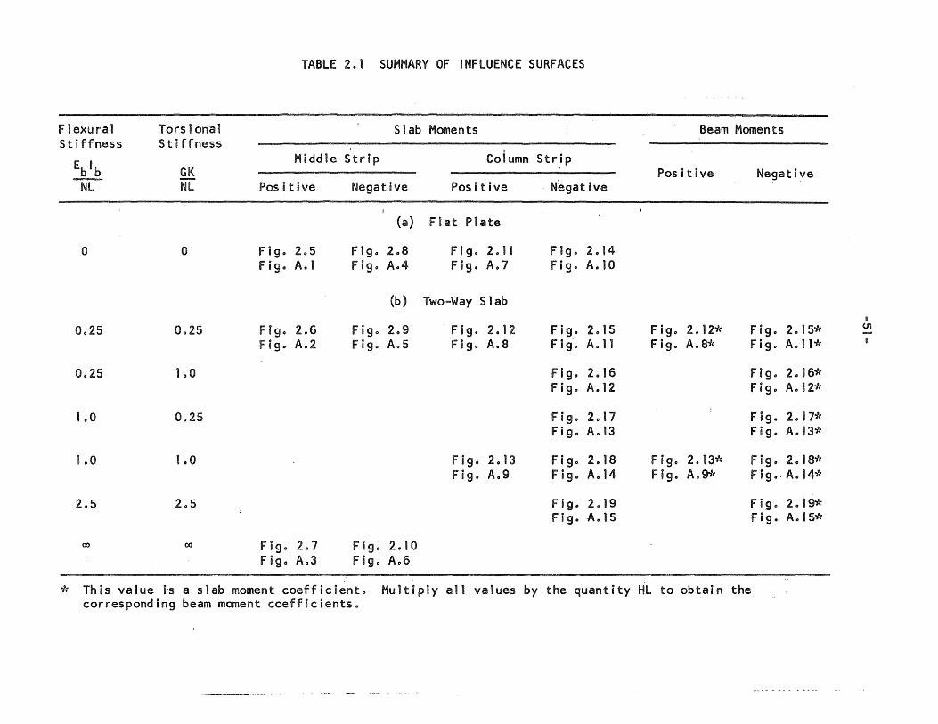
Flexural Stiffness
Eb'b ~
o
0025
0025
100
100
205
00
Torsional Stiffness
GK NL
o
0025
100
0025
1 .. 0
205
00
TABLE 201 SUMMARY OF INFLUENCE SURFACES
Slab Moments
Middle Strip
Positive
Fig. 205 Fig .. A .. l
Figo 2 .. 6 Figo A.2
Figo 207 Figo Ao3
Negative
(a)
Fig. 2 .. B Fig .. A04
(b)
Fig. 209 Fig .. AoS
Fig. 2.10 Fig. A06
I
Column Strip
Positive N:egat ive
Flat Plate
Fig. 2011 Fig. 2014 Fig. A.7 Figo A.l0
Two-Way Slab
Fig. 2.12 Fig. 2.15 Fig. A.B Fig.A .. 11
Fig .. 2016 Figo A .. 12
Fig .. 2 .. 17 Fig. Ao13
Fig .. 2013 Figo 2.18 Fig. A.9 Fig. A.14
Fig. 2019 Fig. A.1S
Beam Moments
Positive Negative
Fig.. 2. 12')" Fig. 2. 15* Figo A08* Fig .. A.,11*
Fig. 2 .. 16* Fig It A. 12')"
Fig. 2 .. 17* Fig .. A.13*
Fig .. 2.13* Fig. 2 .. 18* Fig. A .. 9* Fig ... A (# 14*
Fi,g .. 2019* Fig .. A.15*
* This value is a slab moment coefficient .. Multiply all values by the quantity HL to obtain the corresponding beam moment coefficients.
u U1
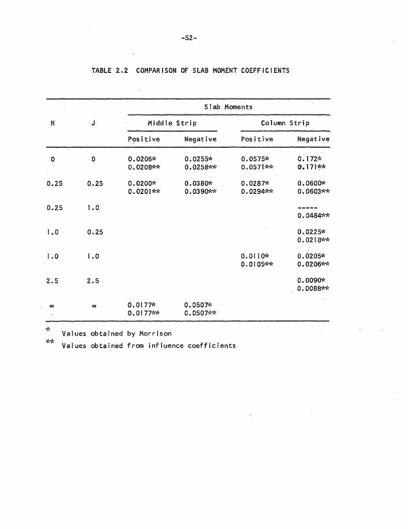
-52-
TABLE 2.2 COMPARISON OF SLAB MOMENT COEFFICIENTS
Slab Moments
H J. M i dd 1 e S tr i p Column Strip
Positive Negative Positive Negative
0 0 0 .. 0206* 0.0255* 0 .. 0575* 00 J 72* 0 .. 0208** 0.0258** 0.,0571** O.171~
0 .. 25 0 .. 25 0,,0200* 000380* 0.0287* 0 .. 0600* 0 .. 0201** o • 039 (P\"* 000294-1."* 000603**
0.,25 1 .. 0 0 .. 0484**
1 .. 0 0.25 000225* 0., 0218-1."')\-
1 .. 0 1 .. 0 000110* 0.,0205* 0.0105-1.,,* 0 .. 0206-1."*
2 .. 5 2 .. 5 0.0090* Oo0088~
co 00 0.0177* 0 .. 0507* 0 .. 0177** 000507-1."*
* obtained by Morr ison Values
** Va1 ues obtained from influence coefficients
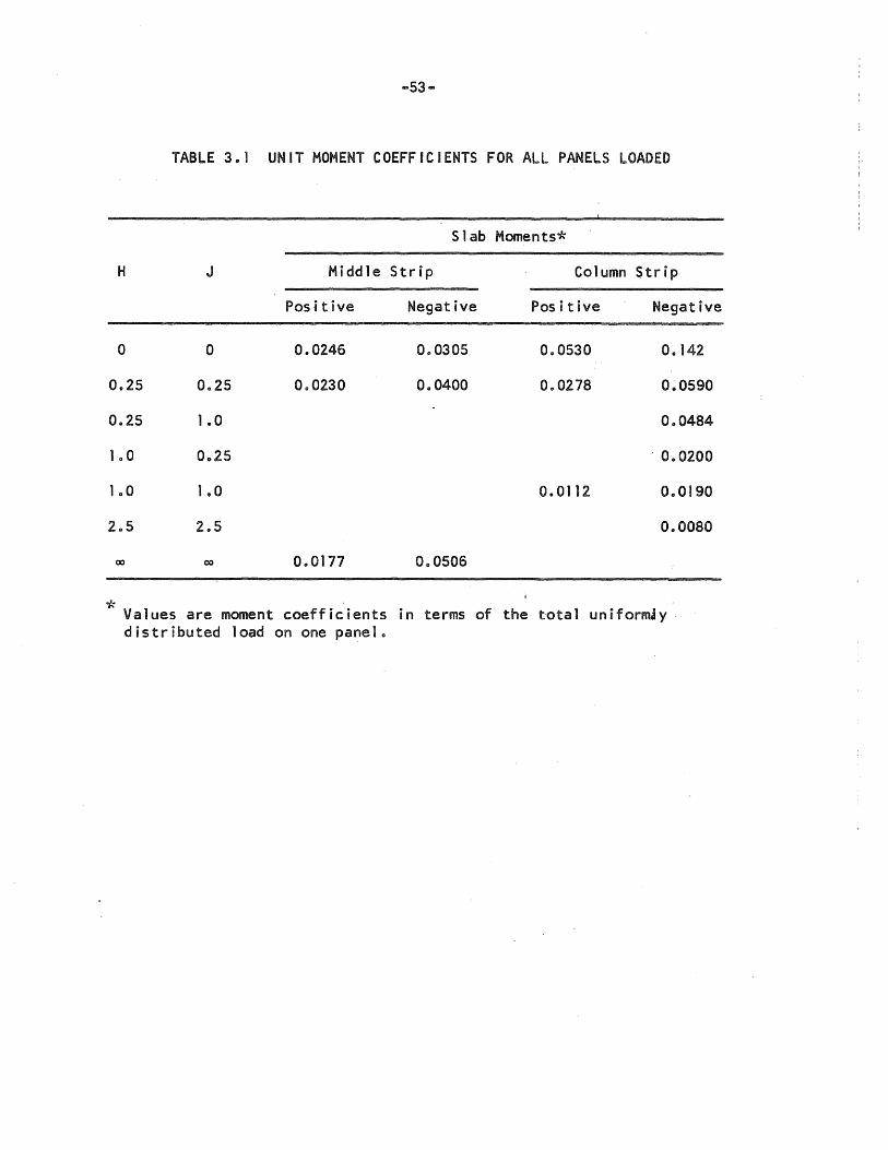
-53-
TABLE 3.1 UNIT MOMENT COEFFICIENTS FOR ALL PANELS LOADED
Slab Moments*
H J Middle Strip Column Strip
Positive Negative Positive Negative
0 0 000246 0.0305 0.0530 O. 142
0025 0.25 0.0230 0.0400 000278 0~0590
0.25 1 .. 0 0.0484
1 .0 0.25 . 0.0200
1.0 1.0 000112 000190
2.5 205 0.0080
00 00 0 .. 0177 0,,0506
* Values are moment coefficients in terms of the total un i formAy distributed load on one panel.
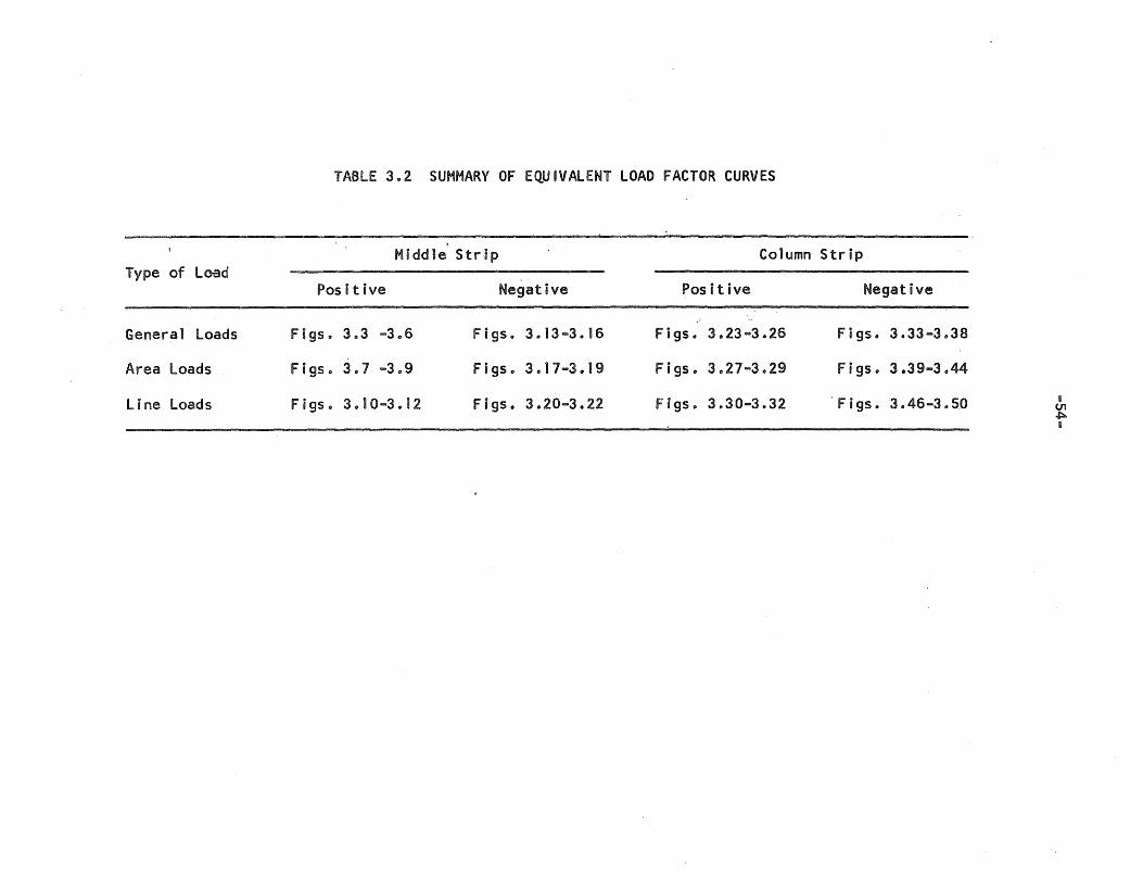
Type of Load
General loads
Area Loads
Line Loads
TABLE 3,,2 SUMMARY OF EQUIVALENT LOAD FACTOR CURVES
Middle Strip
Positive
F i 9S" 3 IS 3 -3 .. 6
Figs.. 3" 7 -3 09
F i 9 s" 3 to 1 0 -3 • I 2
Negative
Figs" 3" 13 -3 .. 16
F i g5.. 3 .. 1 7 -3., 19
Figso 3020-3022
Column Strip
Positive Negative
F i 95" 3" 23 ... 3 " 26 F i 9 s.. 3" 3 3 -3 .. 38
Figso 3027 ... 3029 Figs .. 3.39-3044
Fig s 0 3 0 3 0 ... 3 0 32 . Figs. 3" 46-3050 u VI ~ B
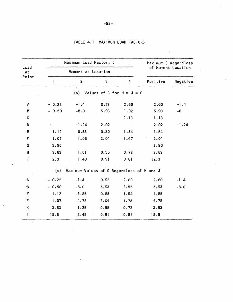
-55-
TABLE 4.1 MAXiMUM LOAD FACTORS
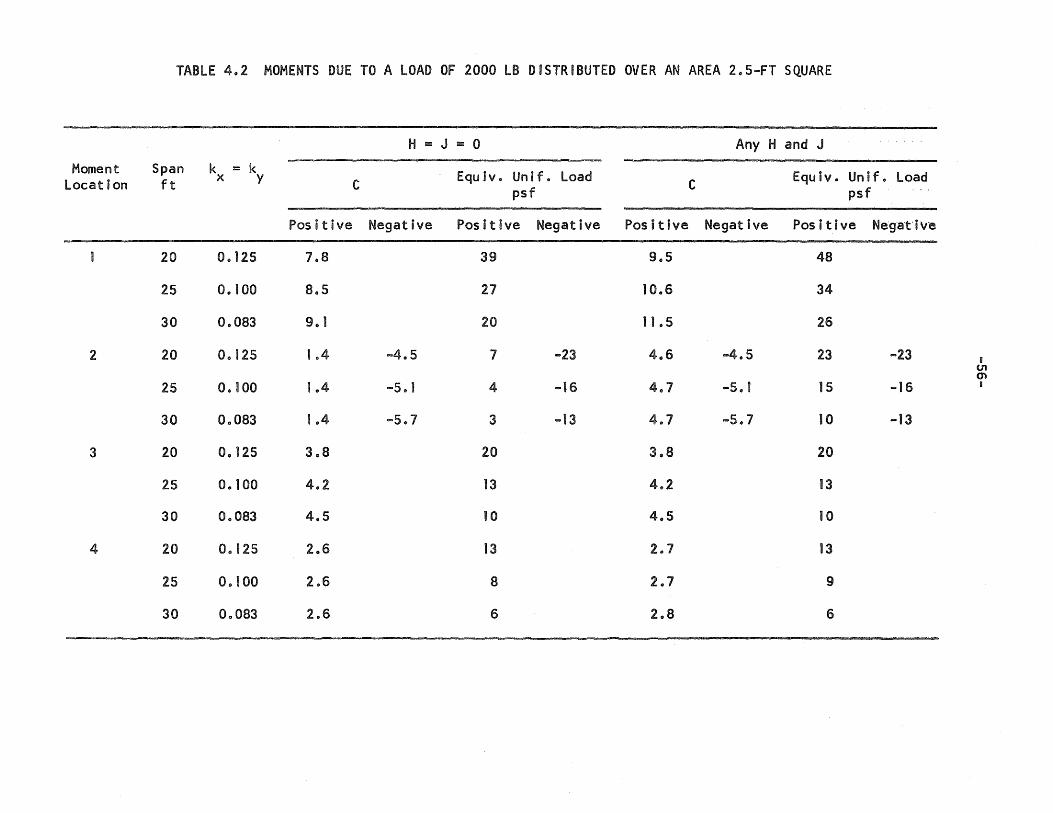
TABLE 402 MOMENTS DUE TO A LOAD OF 2000 LB DISTRIBUTED OVER AN AREA 205-FT SQUARE
H = J = 0 Any Hand J
Moment Span k = k Equlvo Unifo Load Equiv. Unif. Load Location ft x y C C psf psf
Positive Negat ive Positive Negative Positive Negative Positive Neg'at'ive
20 0 .. 125 1 .. 8 39 9.5 48
25 00100 8 .. 5 27 10.6 34
30 00083 9 0 1 20 11 .5 26
2 20 0.125 1 .4 -4 .. 5 7 -23 4.6 -4.5 23 -23 i U'I en
25 0.100 104 -5" 1 4 -16 4.7 -5. J 15 ... 16 D
30 00083 I .. 4 -5 .. 7 3 -13 4.7 -5.7 10 -13
3 20 0.125 3.8 20 3.8 20
25 0.100 4.2 13 4.2 13
30 0 .. 083 4.5 10 4.5 10
4 20 0 .. 125 206 13 2 .. 1 13
25 0 .. 100 2.6 8 2.7 9
30 00083 2 .. 6 6 2 .. 8 6
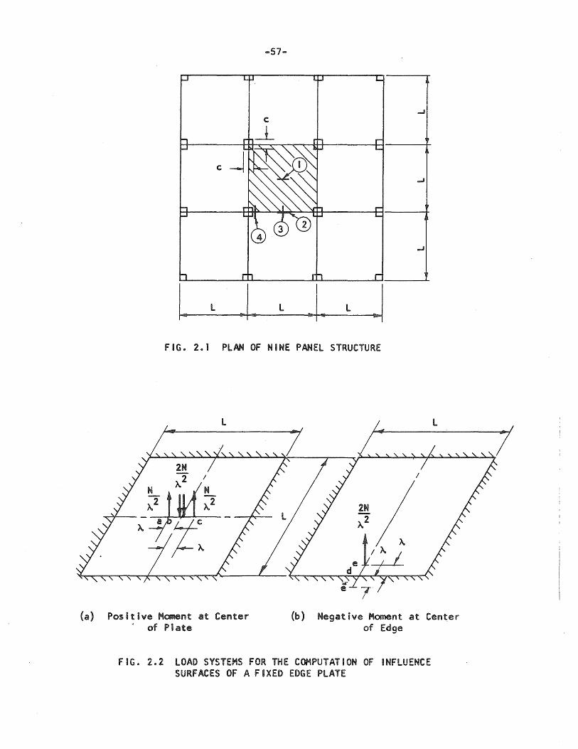
-57-
...J
I~ L .1. L L
FIG. 2.1 PLAN OF NINE PANEL STRUCTURE
L L
(a) Positive Moment at Center of Plate
(b) Negative Moment at Center of Edge
FIG. 2.2 LOAD SYSTEMS FOR THE COMPUTATION OF INFLUENCE SURFACES OF A FIXED EDGE PLATE
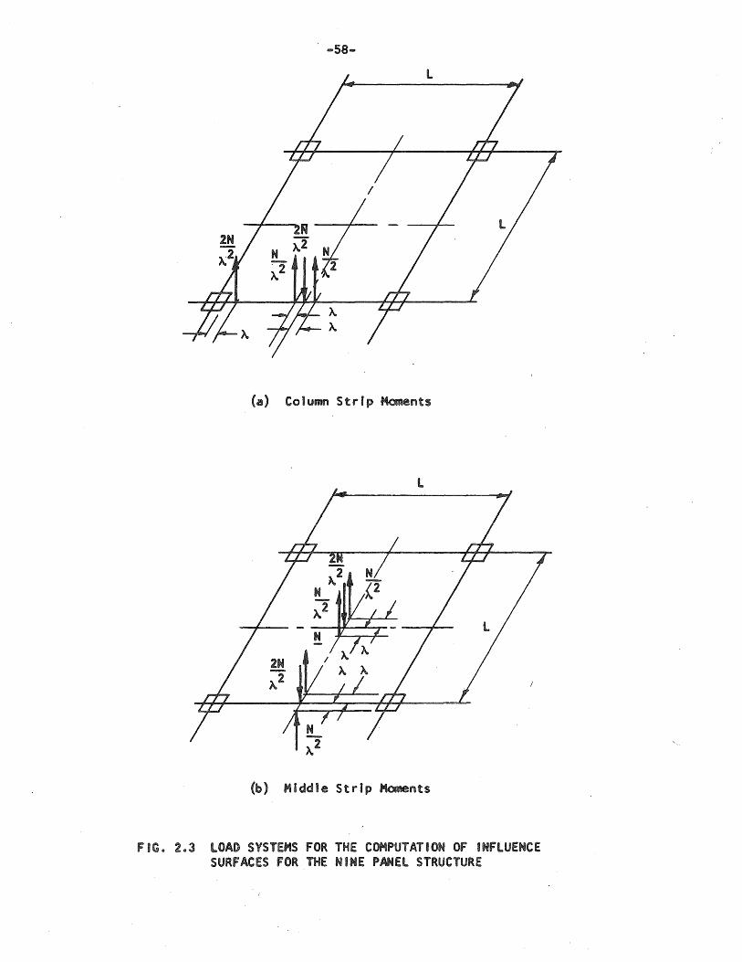
-58-
(a) Co1umn Strip Moments
L
(b) Middle Strip Moments
FIG. 2.3 LOAD SYSTEMS FOR THE COMPUTATION OF INFLUENCE SURFACES FOR THE NINE PANEL STRUCTURE
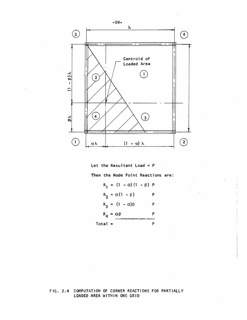
-co..
'"e
... 59 ...
Centroi d of loaded Area
(1 ... a) ")..
let the Resultant Load = P
Then the Node Point React ions
R) I: (1 ... a) (1 .. t') P
R2 = 0(1 ... p) P
R3 == (1 ... a)t) P
R4 B at) p
Total I!II: P
CD
are:
FIG. 2.4 COMPUTATION OF CORNER REACT'ONS FOR PARTIALLY LOADED AREA WITHIN ONE GRID
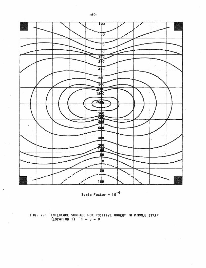
.... 60 ....
-4 Scale Factor = 10
FIG. 2.5 INFLUENCE SURFACE FOR POSITIVE MOMENT IN MIDDLE STRIP (LOCAT. ON 1)' . H = J == 0
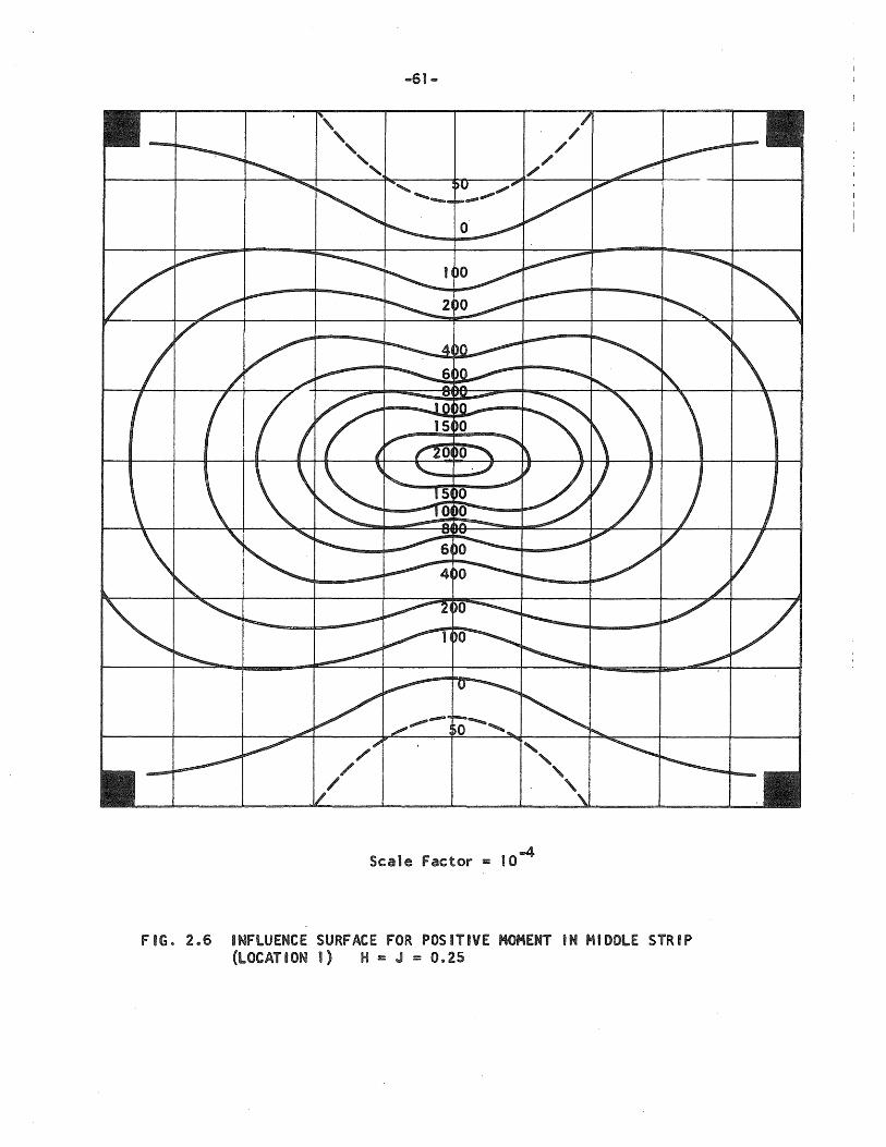
-61-
4 Scale factor = 10
fiG. 2.6 INfLUENCE SURfACE fOR POSITIVE HOMENT IN MIDDLE STRIP (LOCATION 1) H = J = 0825
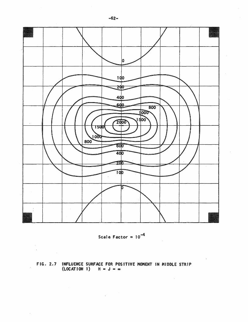
Scale Factor == 10,-4
FIG. 2.1 INfLUENCE SURfACE FOR POSITIVE MOMENT IN MIDDLE STRIP (LOCAT I 1 ) H - J - •
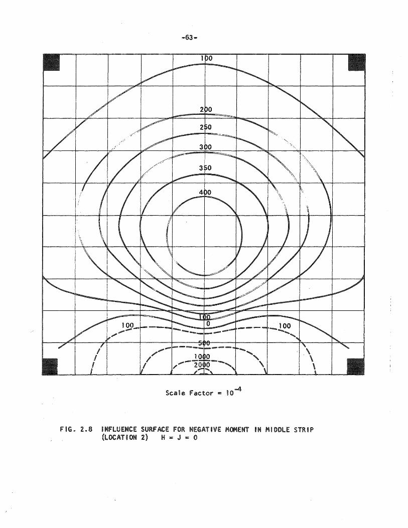
-63 ....
-4 Scale Factor = 10
FIG .. 2 .. 8 INFLUENCE SURfACE fOR NEGATIVE MOMENT IN MIDDLE STRIP (LOCATION 2) H = J = 0
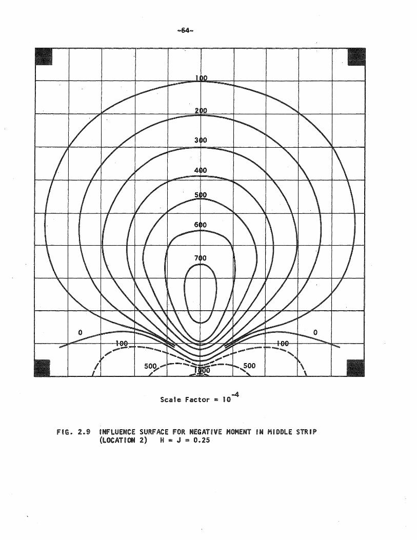
~ Scale Factor ~ 10
FIG. 2.9 INFLUENCE SURFACE FOR NEGATIVE MOMENT IN MIDDLE STRIP (LOCATION 2) H = J = 0.25
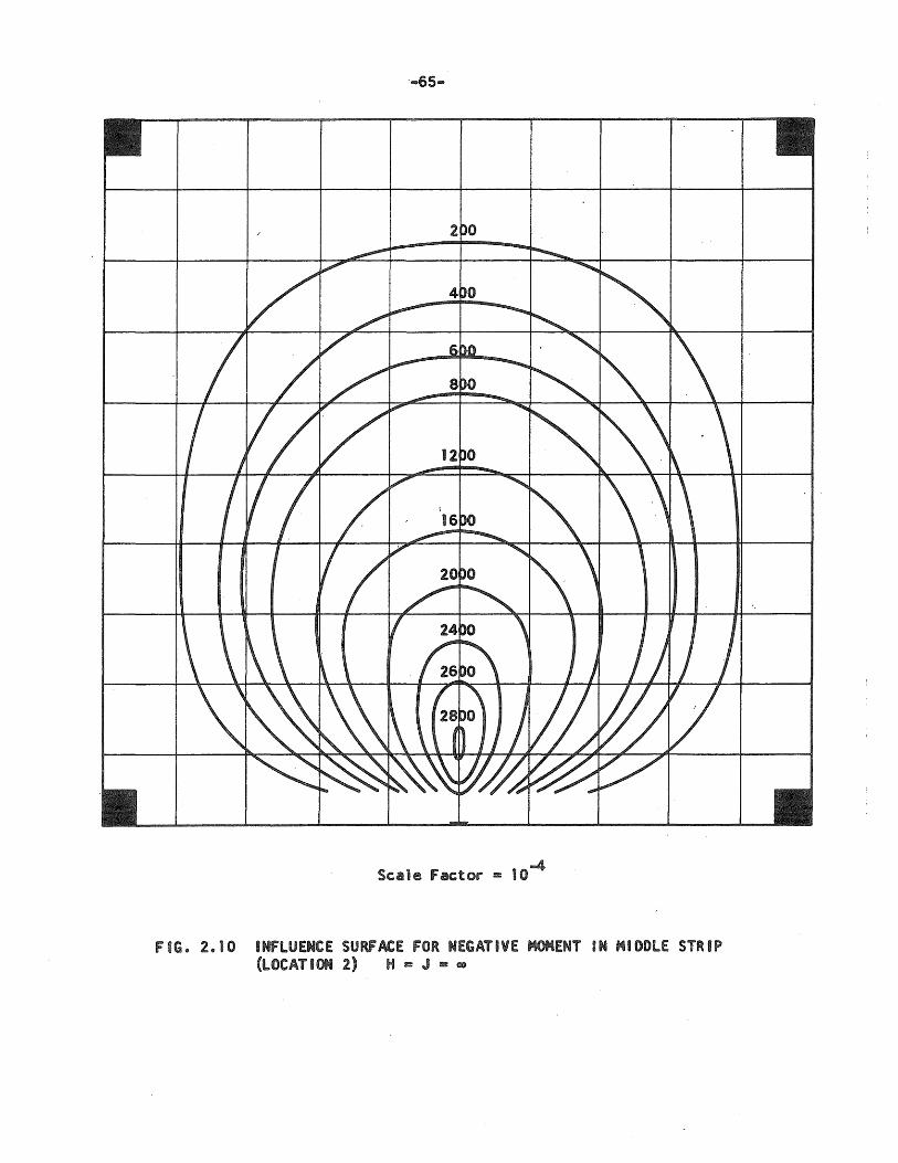
-4 Scale factor = 10
fIG. 2.10 INfLUENCE SURfACE fOR NEGATIVE MOMENT IN MIDDLE STRIP (LOCATION 2) H = J = ~
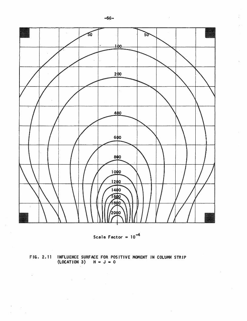
4 Scale factor u 10
fiG. 2.11 INfLUENCE SURfACE fOR POSITIVE MOMENT IN COLUMN STRIP (lOCATION 3) H c J - 0
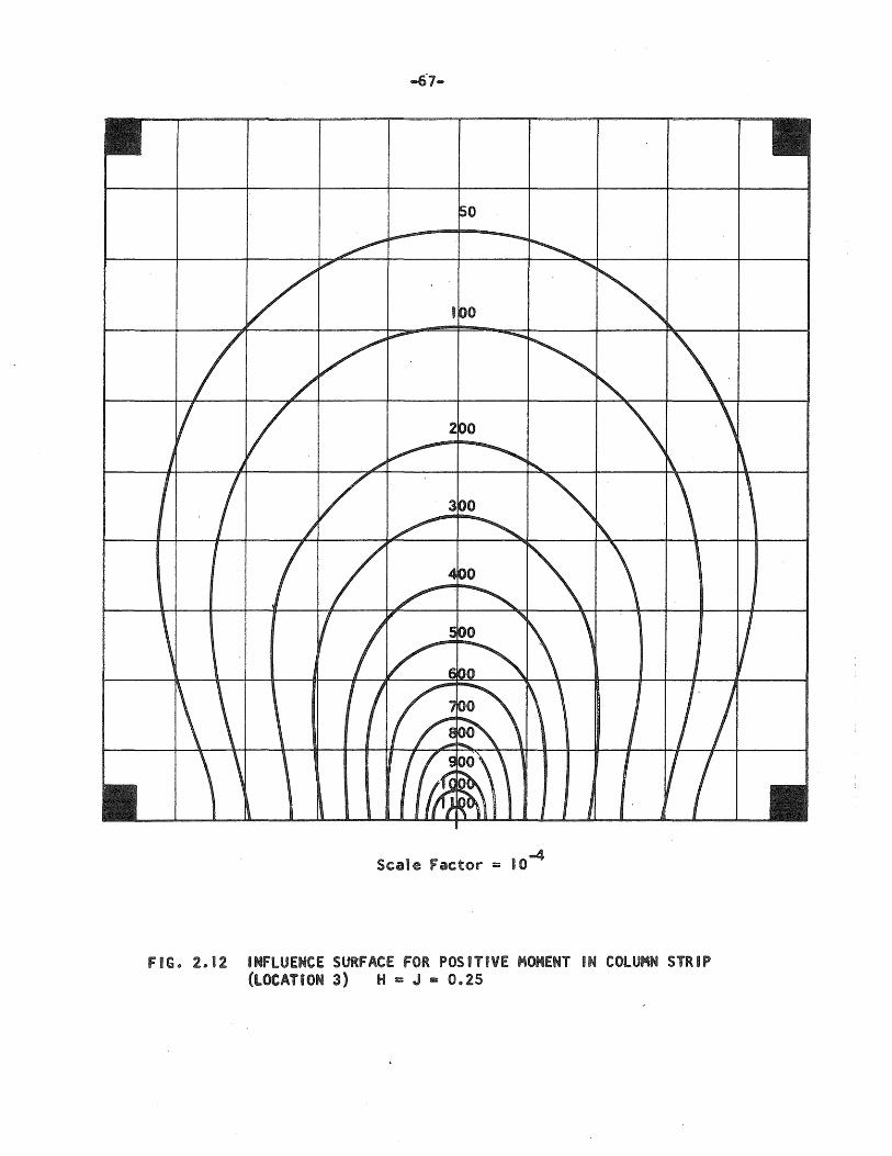
4 Scale Factor = 10
FIG. 2.12 INFLUENCE SURFACE FOR POSITIVE MOMENT IN COLUMN STRIP (LOCATION 3) H = J - 0.25
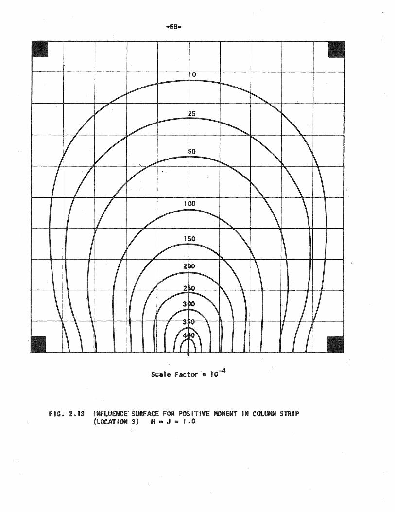
fiG. 2.13 INflUENCE'SURfACE fOR POSITIVE MOMENT 8N COlUMN STRIP (lOCATION 3) H,. J l1li 1.0
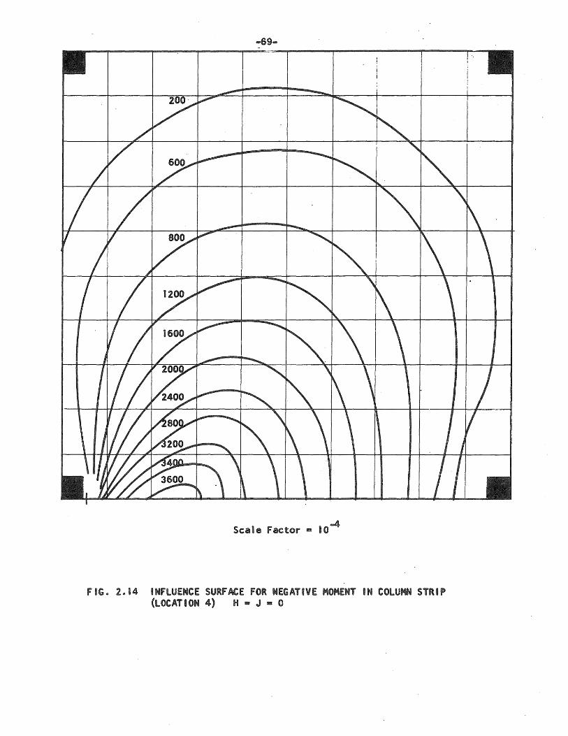
Scale Factor _ 10-4
FIG. 2.14 INfLUENCE SURFACE FOR NEGATIVE MOMENT IN COLUMN STRIP (LOCATION 4) H - J • 0
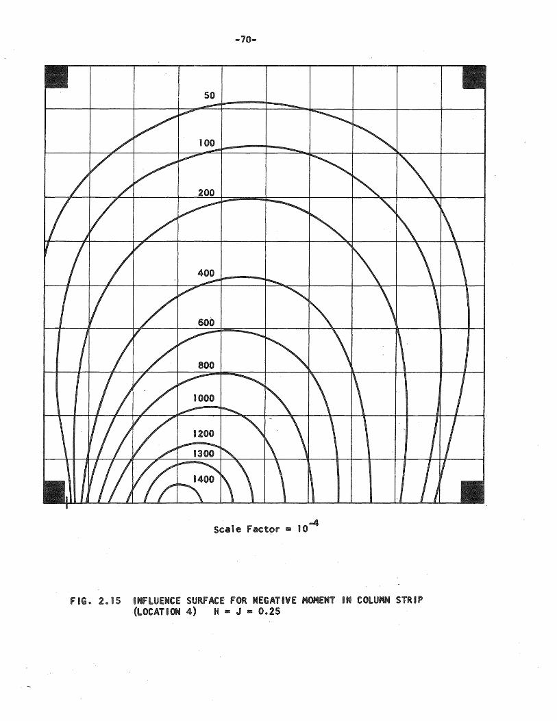
-70-
50
~ Scale Factor c 10
FIG. 2.15 INFLUENCE SURFACE FOR NEGATIVE MOMENT IN COLUMN STRIP (LOCATION 4) H - J = 0.25
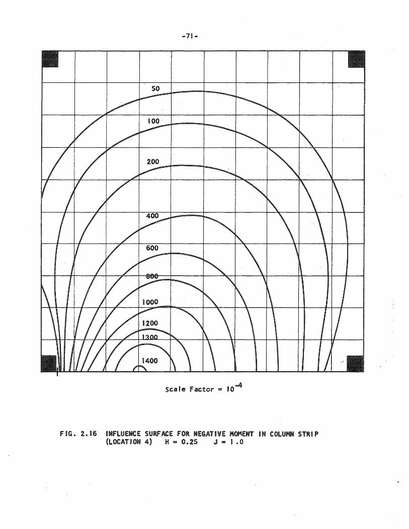
... 71- ...
fIG. 2.16 INfLUENCE SURfACE fOR NEGATIVE MOMENT IN COLUMN STRIP (LOCATION 4) H. 0.25 J • I .0

10
-72-
-4 Scale factor !E 10
FIG. 2.17 INFLUENCE SURfACE fOR NEGATIVE MOMENT IN COLUMN STRIP (lOCATION 4) H. 1.0 J - 0.25
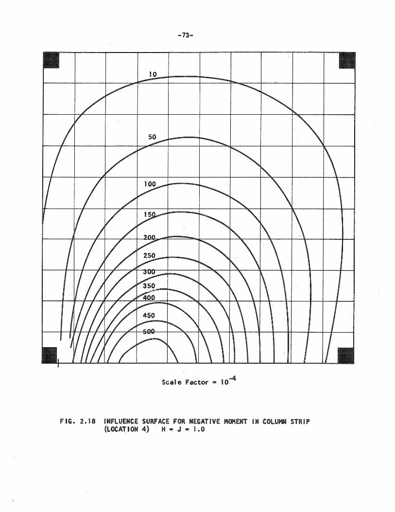
4 Scale Factor - 10
FIG. 2.18 INFLUENCE SURFACE FOR NEGATIVE MOMENT IN COLUMN STRIP (lOCArION 4) H - J = 1.0
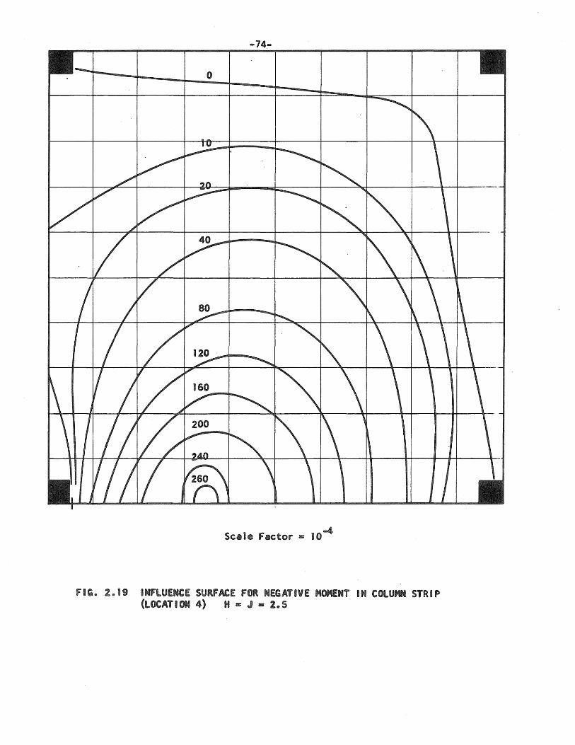
... 74 ....
o
Scale Factor = 10-4
FIG. 2.19 INfLUENCE SURFACE FOR NEGATIVE MOMENT IN COLUMN STRIP (LOCATION 4) H - J - 2.5
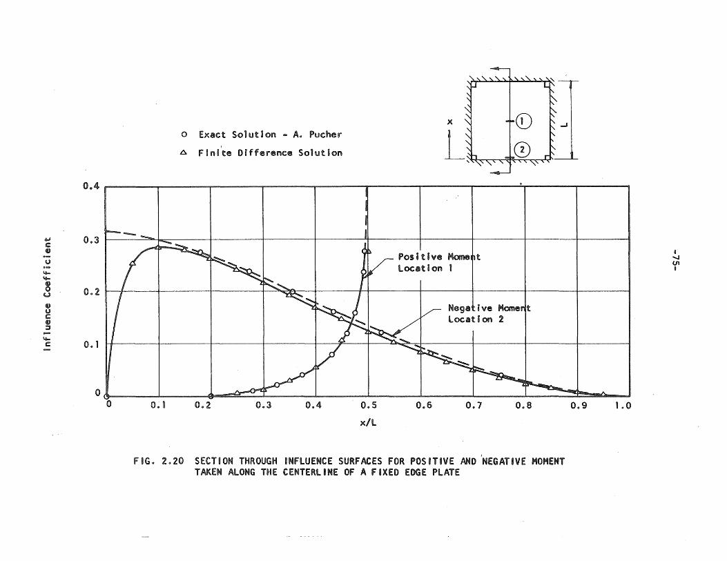
4J c ~ .-u .... ~ 11.6-
8 u ~ u c Q) :J -~ c
0.4
0.3
I IT 0 .. 2
II o. 1
o Exact Solution - A. Pucher
6 Flni~e Difference Solution
x
~'nl ~/ Posl't!ve Homeft Locat I on 1
~~I ~ Negative Moment locat f on 2
...J
o & JJ ~ =-+:: '\ o O~ 1 0 .. 2 0 .. 3 0.4 0.5
x/L
0 .. 6 0.7 0.8
FIG .. 2.20 SECTION THROUGH INFLUENCE SURFACES FOR POSITIVE AND INEGATIVE MOMENT TAKEN ALONG THE CENTERLINE OF A FIXED EDGE PLATE
0.9
I .....s U'i B
1 .0
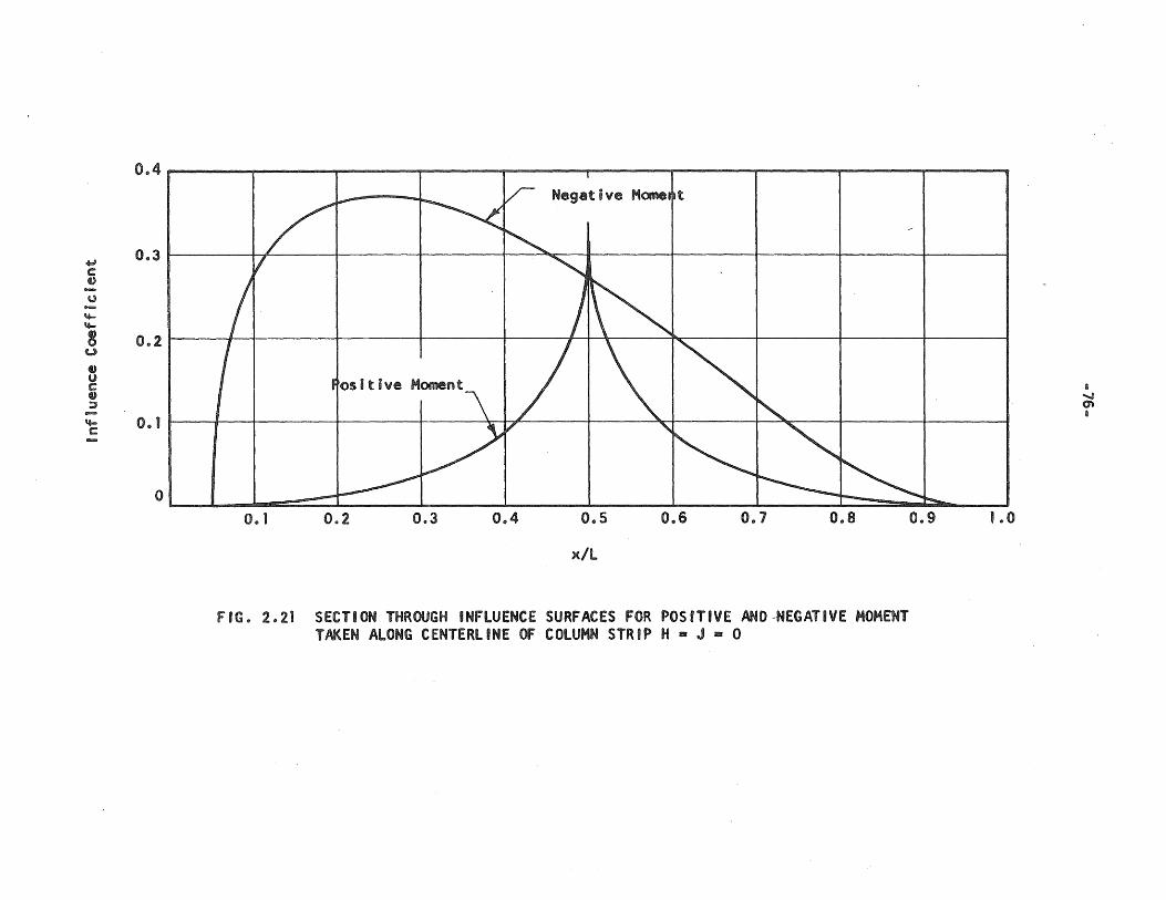
4.D C ~
U
'4-I.e-
8 u e» u c Q) ::JI
~ C
0.,4
Negative Homen.t
....... 0 .. 3 I I A' ~
0 .. 2 I I : '... ~
os I t Ive Homent-"
\. .I '<I , 0 .. I I to I»
O':J r :t'>a 0 .. 1 0 .. 2 0.3 0 .. 4 0 .. 5 0 .. 6 0 .. 1 0 .. 8
x/L
FIG. 2.21 SECTION THROUGH INFLUENCE SURFACES FOR POSITIVE AND~EGATIVE MOMENT TAKEN ALONG CENTERLINE OF COLUMN STRIP H a J = 0
0.9 1 .. 0
8 ....., m a
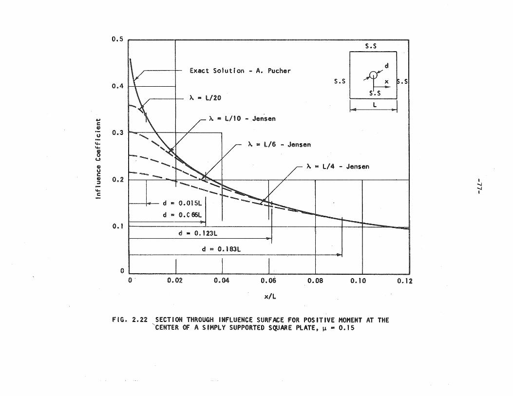
4.D C ., U
~ '+-
8 u Cl) u c t) ::J
'+C
0 .. 5
Exact Solution - A. Pucher
0.4 ~I~'~---------
A SII L/20
- Jensen
O.l
~ - l/G - Jensen
"<sL. , ..... <:::----'~- 7£
I >If d fIIII:: 0 .. 01 5L
0. 1 ~ O.C~~I ~~
d = 0.123l _I ~I
d = 0.D8ll
s.s
d
5.S I ~ ~.S S.S
1=41 L ~ I
- Jensen
01 ____ ~ __ ~ __ ~ __ ~ __ ~ __ ~ 0' 0 .. 02 0.04 0.06 0.08 0.10
x/L
FIG. 2.22 SECTION THROUGH INFLUENCE SURFACE FOR POSITIVE HOHENT AT THE 'CENTE:R OF A S .HPl Y SUPPORTED SQUAR.E PLATE, fJ. m 0 .. 15
0.12
o ...... ...... a
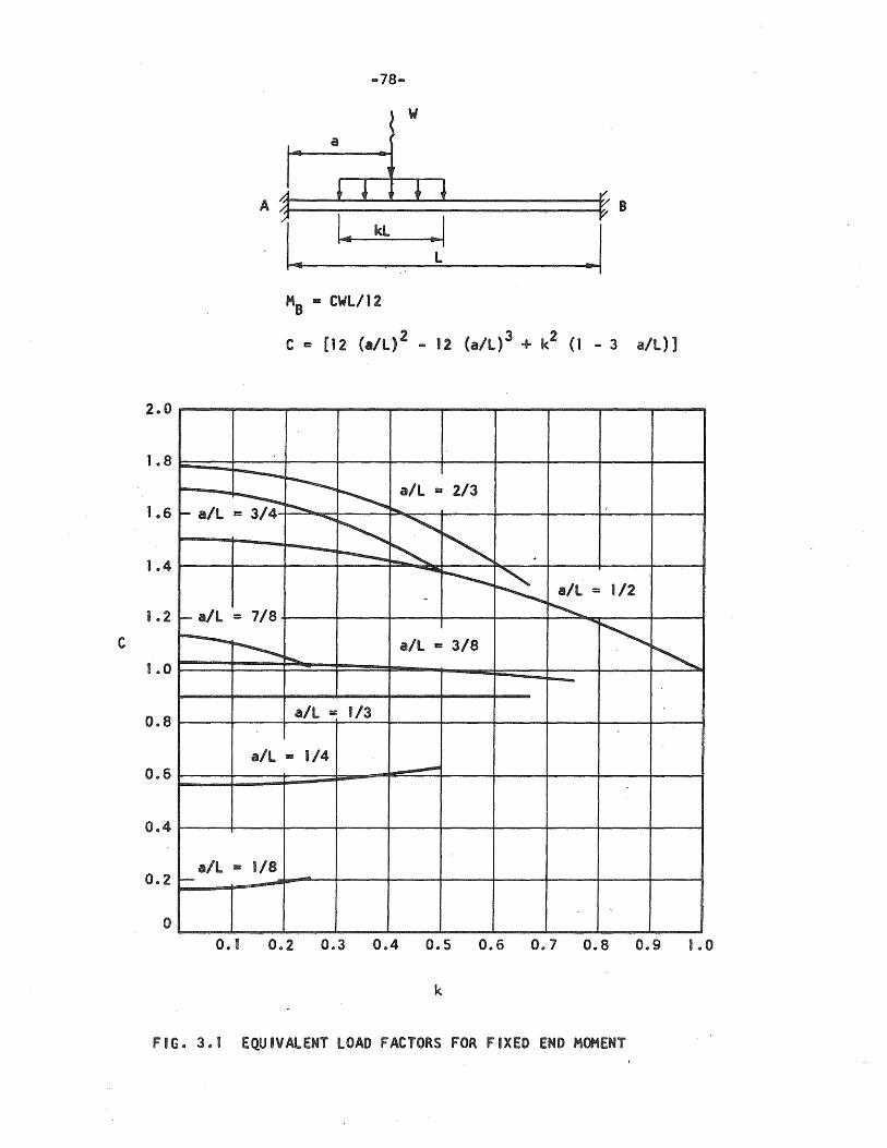
... 78 ...
A /~ __ ~ ________________ ~ __ -+/ e kl
.1 l
He lIZ CWl/12
C I: [12 (a/l')2 ... 12 (a/l)3 + k2 (1 - 3 aIL)]
2 .. 0
1.8
1 .. 6
J .. 4
1 ,,2
C
1 .. 0
~ ~ ..... ~
aIL = 213 ~ ~ ....... ~ all I: 3/4 .........
~ ;'~ - ---- ......,.,. ~ ~ all = 1/2
r- all = 7/8 ~
----.....~ ~~
all I: 3/8
" ...... -
0 .. 8 all = 1/3
all - 1/4 0,,6 ...-..
0 .. 4
0 .. 2 aIL - 1/8 -
0
0 .. 1 0.2 0.3 0.40.5 0.6 0.7 0 .. 8 0.9 1.0
k
FIG. 3.1 EQUIVALENT LOAD FACTORS FOR FIXED END HOMENT
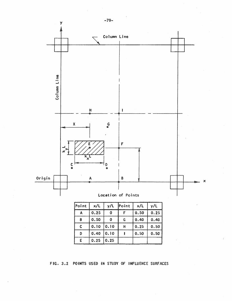
y -79-
A.
"" Co 1 umn LI ne
CD c
I -.....B
C e j -0
u
H I - III - -
I X G .. ct -
.
~{~. F
C l• x .10 I • CD
Origi"n J
. I A B , -Lt-J
-
t i on of . Loea POints
Point x/L y/L Point x/l
A 0 .. 25 0 F 0.50 0.25
B 0 .. 50 0 G 0 .. 40 0 .. 40
C 0 .. 10 0 .. 10 H 0 .. 25 0.50
D 0',,40 0 .. 10 0 .. 50 0 .. 50
E 0.25 0 .. 25
FIG .. 3 .. 2 POINTS USED eN STUDY OF INFLUENCE SURFACES
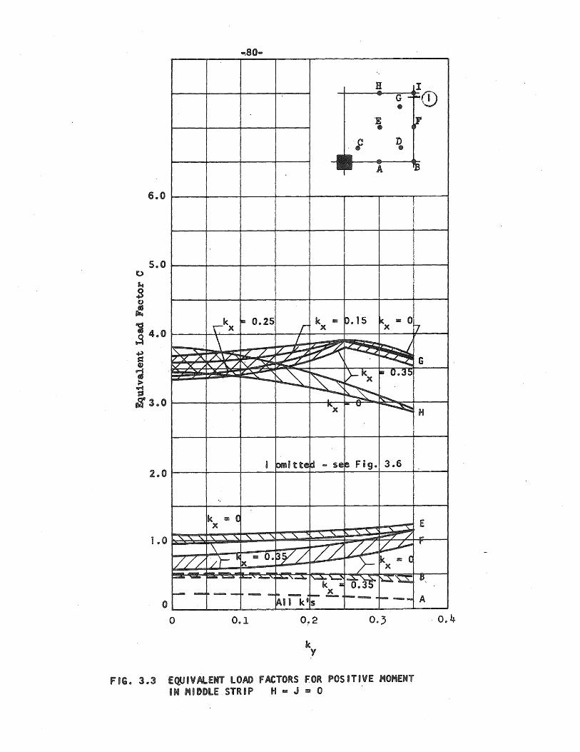
o J.4
3 t)
&!
H I
A
5.0r----r--~~--~--~----~--~----~--~
il 34.0r---~r-~--~--~~--+---~--~~~
11 Q>
';j
~ ~3.0r---+---~---+---4~~~~~~~--~
Fig. 3.6 2.0r----r--~----~---4----~--~----~--~
o 0 .. 1
k Y
FIG. 3.3 EQUIVAlENT LOAD FACTORS FOR POSITIVE MOMENT IN MIDDLE STRIP H - J = 0 .
. 0.4
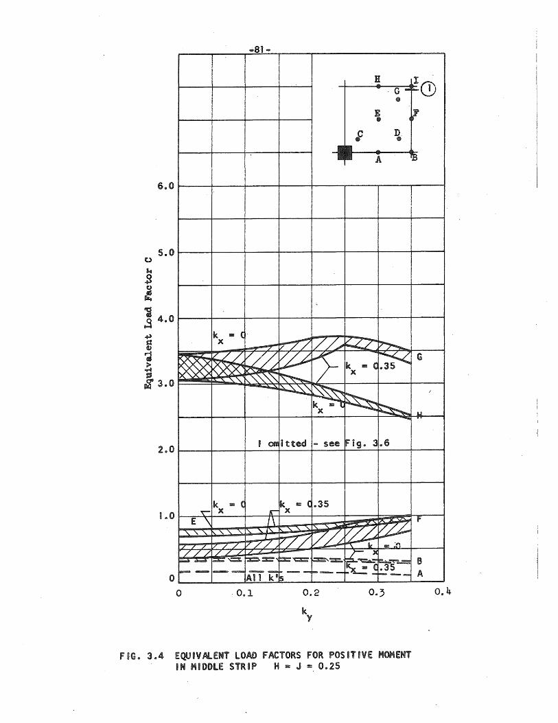
-81-
H \.1) ·G CD
E CD
f D. CD
A
6.0~--~----~--~--~--------~----~--~
5.0~--~----~--~--~----4----4----4---~
o 0.1 0.2
k Y
0.3
FIG. 3.4 EQUIVAlENT LOAD FACTORS FOR POSITIVE MOMENT IN MIDDLE STRIP H ~ J = 0.25
0 .. 4
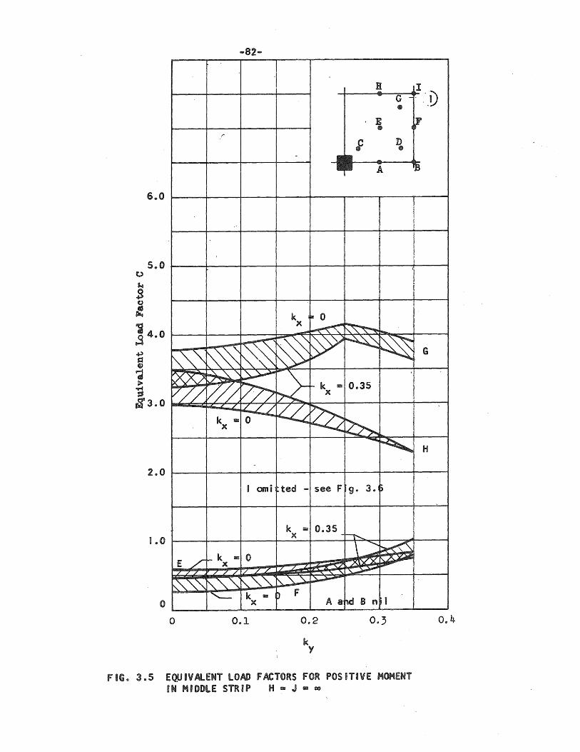
,
6 .. 0
I
~
~ to ~~ RQY< ~'\ ~
V7/ ~ V/7 / ///
k - o -x
-2 .. 0
I omi
J .. 0 _ k :: 0 E/ x
/ / 7// / / /'
r--..." "" ~'" " ~"" k -x
o 0 .. 1
-
k I: 0 X --~ ~ 8>Y ~ f- k == x
~ ~
ted ... see F
k = 0.35 _ x
~ P F A a
0.2
k Y
H I .... G -- ,'0 . -
E I~ • ; D •
... A ~
I I
! I
I , i
-,,~ ..... ~ ~ G
0.35 I
~ H
g .. 3.1)
~
~ ~d B n I
FIG. 3.5 EQUIVAlENT LOAD FACTORS FOR POSiTIVE MOMENT IN MIDDLE STRIP H == J • ~
0.4
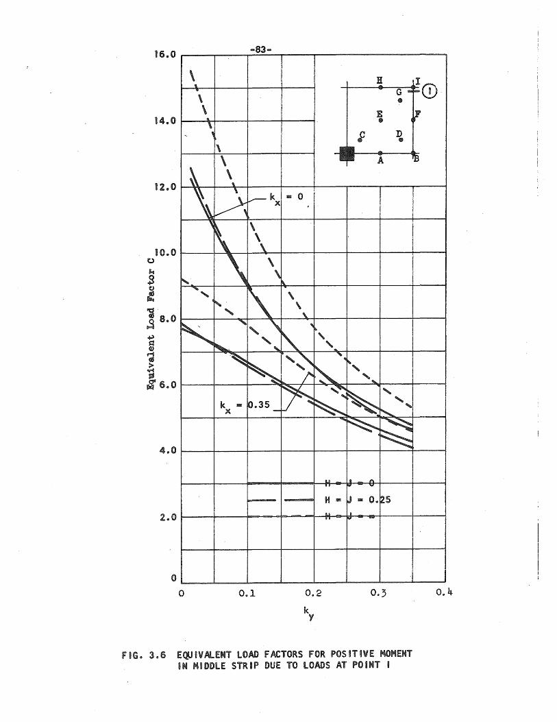
o ~
$ o :
16.0 -83-
\ H 10 \ \ E
14.0 • ~ D •
A
12.0
10.0~--~~-+~~~--~---r--~----~--~
4.0~--~---+----+---~---+----+---~--~
o 0.1 0.2
k Y
0.4
FaG. 3.6 EQUIVAlENT LOAD FACTORS FOR POSITIVE MOMENT IN MIDDLE STRIP DUE TO LOADS AT POINT I
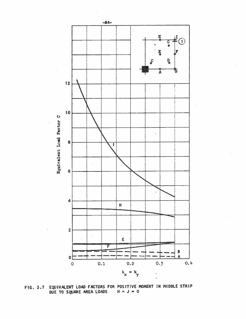
I H I .... G ~r-CD
~ • 'E •
IF . ~ .
f D • -A ~
12 \
\ I I 1
I 1 ?
10 t,)
s.. .s
\ I 1\ ;
\ ! i I
I \ !
C)
~ ~ 8 3 ~ Q OJ
\
1\ I
'\ ;
l I
I\. I I
~ > ~
=' g 6 "'~ i i
. ! .~
~ I I
" N H
1
i ---....-.. .... j
4
l 2
E
f I
- -.. ........ "--.... _- B o r-- .............. I- --
.................... ........ ,- ~............, -- -- ..... A
o 0 .. 1 0.2 0 .. 4
k - k x y
FIG. 3.1 EQUIVAlENT LOAD fACTORS FOR POSITIVE MOHENT IN MIDDLE STRIP DUE TO SQUARE AREA LOADS, H = J - 0
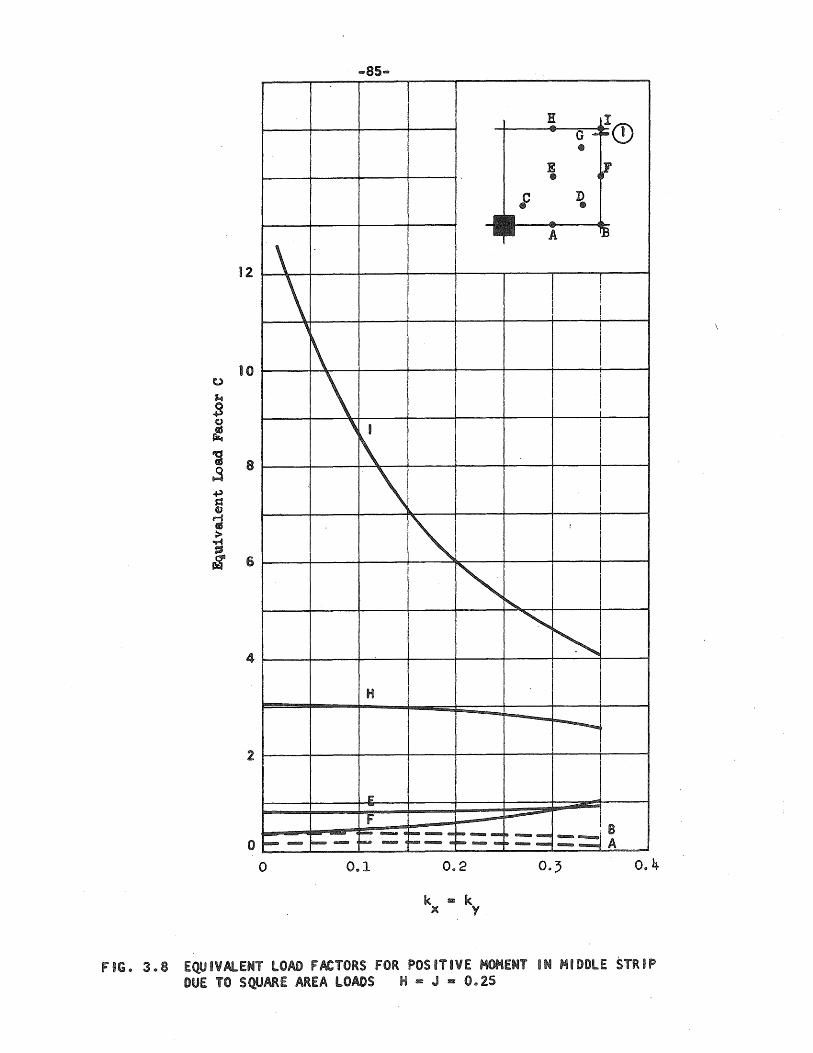
... 85 ....
H I ... G .... ~Q) •
E 47 • ; D •
-A 1B
12 \ \ I
, 1 I !
10 t,)
~
.s
, !
~ I
\ I CJ
~ 'i 8 3 ~ s::: QJ
, I
I
\ !
\ II > ..... ~
~ 6 ~ :
~ ~
" ~ I
4
H I
----....... 2
C' J F I ........... F- ............. 10--_ 1--- =:jB --I-- - 1-- 1-"'-' tz-. ........... """"- ...... 1--- ......... A
o 0 .. 1 0 .. 2 0 .. 4
k lIiC k x y
FIG .. 3 .. 8 EQUIVAlENT LOAD FACTORS FOR POSITIVE MOMENT IN MIDDLE STRIP DUE TO SQUARE AREA LOADS H lIiC J - 0.25
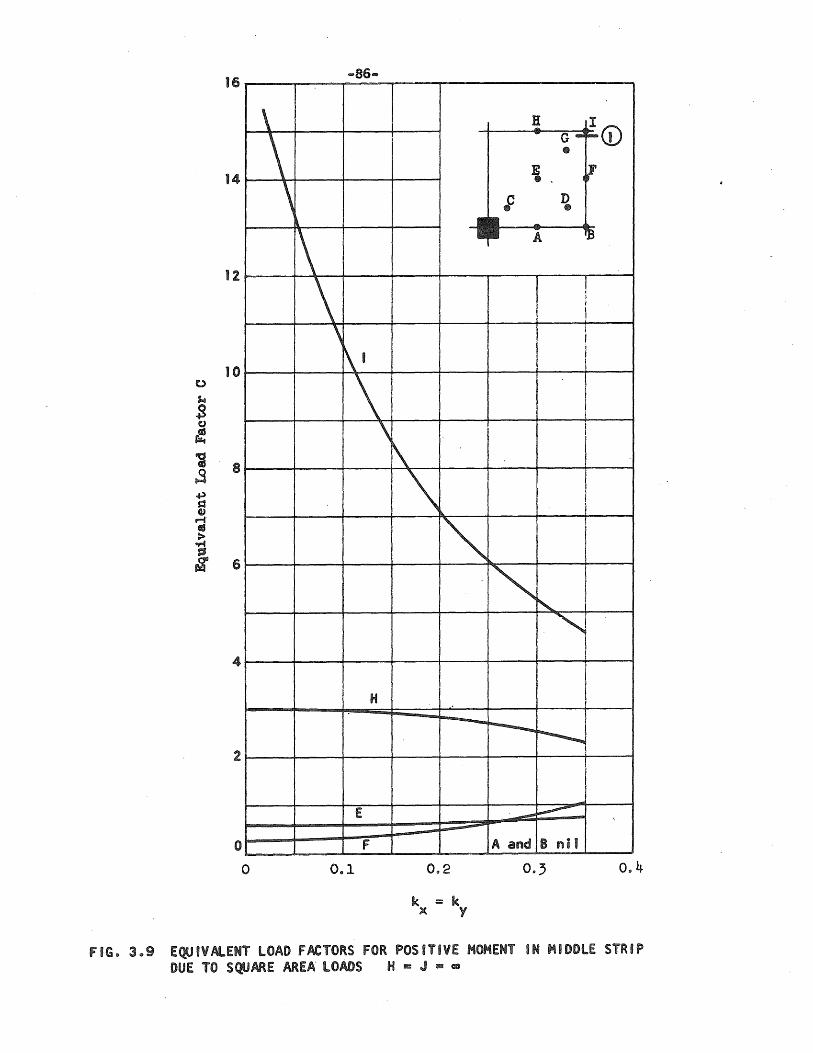
t>
~ .s ()
rf 'i ..9 +> s::3 Q,)
.....c IS >-
"1"4 ~
$
16
14
12
10
8
6
4
2
o o
\
'\ \
l
~ \ ,
f\1
\ \
H
E
f
0 .. 1
H I I G-~Ci)
• E ~~., • •
.C D • .... A B
! )
i I I
l I I
I I
I
" I
\ I I
"" .", "-
---..
0.2
k = k x y
r----..
-A and
" ~
~
8 ni I
0 .. 4
fIG. 3 .. 9 EQUIVAlENT LOAD FACTORS FOR POSITIVE MOMENT IN MIDDLE STRIP DUE TO SQUARE MEA' lOADS H - J II1II 00
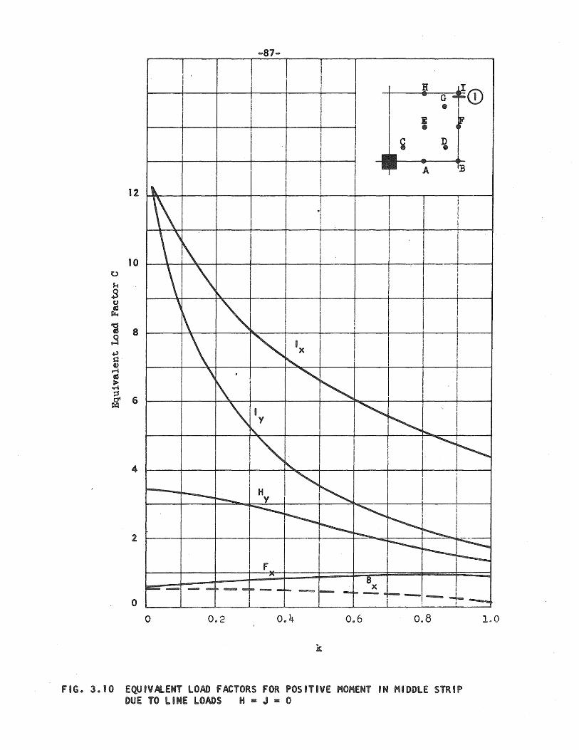
!ID87 ....
I , I I 1 J I
~ J I
I I - G --CD
1 • I I I 4r ..
I ~ ~ I
! ...
! - B A
I
12 \. ! I
\\ I ! I ,,/ i i I
I i \ \ \ . I I
I I
1\ j ! I I
I I
\1 \~ I !
i
I I I
10
, '" I
I \ 1 \ '" 'x I I
I I
"- , I \ .
" . I
I
~ I
\ I - ! i
\ • ~ I y
" I ~ ~ 1
'" I~I . ~ ,
I
I ""'I~ i - H I -~ r--...... y I
4
~
---""""--.. ~ I
~ I I
r---. ~!
I -~ ~-
~r----F
2
" Bx
~- - ...... "'--Fa- ...... I'- --- I i"'"='=== ---........... -- - -'-, i --.... o
o 0 .. 4 0 .. 6 0,,8
k
FIG. 3.10 EQUIVALENT lOAD fACTORS fOR POSITIVE MOMENT IN MIDDLE STRIP DUE TO LINE lOADS H - J - 0
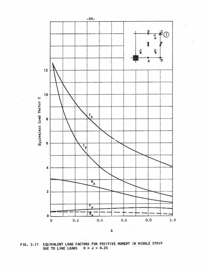
... 88 ...
I i B II I "'" G ... ,...,@
• I ~r
~ D • I "'"
12
-I - TB
,~ A
I
I
\\1 I l \
!
\ 1\ I , I
I
\ f----'-; t
r\. I :
10
,
'" j
~ I I i\..X ! --
'\ '" ! I
~ I i
\ '" I ~ 1'., I
~ ,
" 1
I
~ I i
~ ........
~ '" "'-
I --- ./
-~ H ........
~ +-_ ...... -
r---... ;
~ ~ ~ - Foo... --'-""-..............
~ --..... ~
~ t----
4
2
--fx
~ .......... 1--~- iTx-- -- -- ... ~ .......... to-- ............ - ....... ~--o o 0.2 0.4 0.6 0.8 1.0
k
FIG. 3.11 EQUIVALENT LOAD FACTORS FOR POSITIVE MOMENT IN MIDDLE STRIP DUE TO LINE LOADS H B J B 0.25
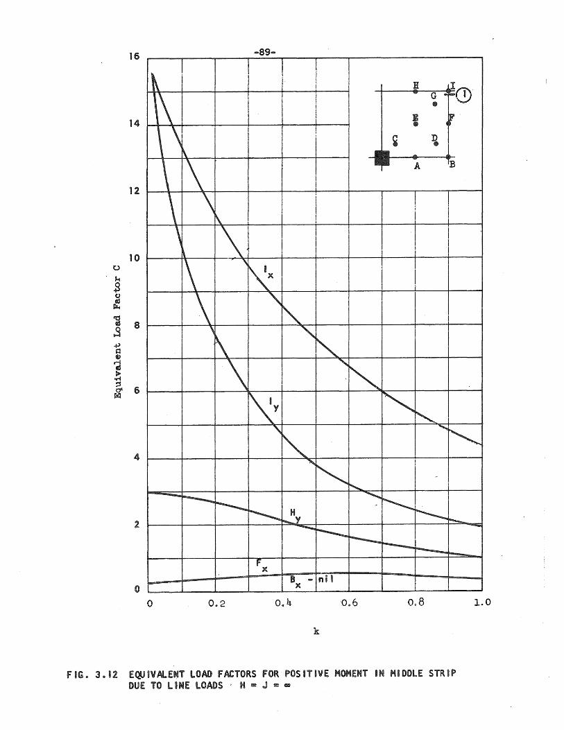
16 -89 ...
14
I I I
'\ ! I
! ! II LI .
l\ ! ....
G -'"-CD j fit
I E r I
\ \ ! (I
I ~ D
fit
~ ....
\ \ - B A
\ \ i I I
~ I
i
12
\ \ ~
\ ''(X 10
\ " " , "-\ " \ '" ~ I\y '" '" " ~
~
" " "'- -, 4
--... ~ ..............
~ ~ ~ H ~ ~y """-.
~
~ -~ r----. r---...
2
Fx !'"
B .... nil x o
o 0 .. 2 0,,4 0.6 1.0
k
FIG. 3.12 EQVIVAlE"T LOAD FACTORS FOR POSITIVE MOMENT aN MIDDLE STRIP DUE TO LINE LOADS' H - J z ~
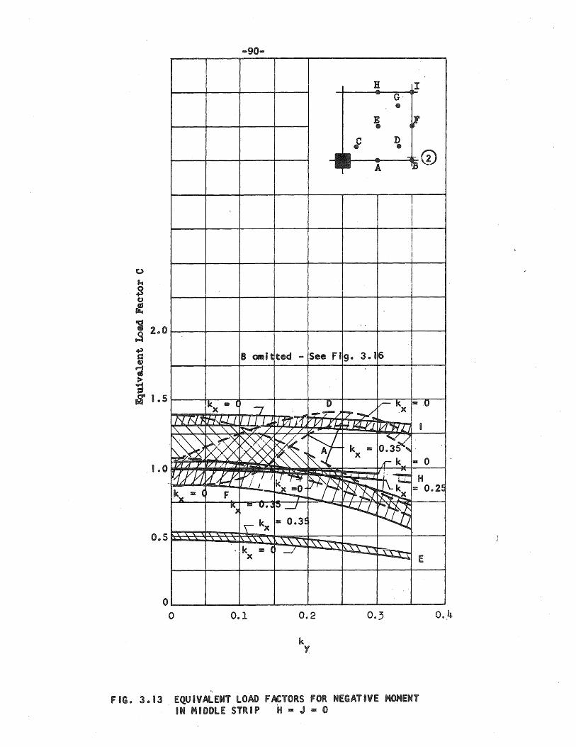
7'[7::!'f. " '\. '\.
.~ . 1 .. 0
·'17171 l'
J{fJ1 k :m« ~)(
0 .. 5 I
... go ....
Ii I "" G
• E ~ •
f D • .- ~t-. G) A B
I I I , !
I
I
8 omit ted - See Fi g .. 3 .. 16
!k, - ( 7
-n V- ~x - .0 X -..,......od! -~// t"7_~ 'RJ::l1 I111 U ~{ffJ1 .[7} .£/..4 U f4,.J/J '\. ,,'\. ~/ / / / /.:.. II/I"'H I J I
~ ~ ~W ~ " k !III: 0 ... 35 I: x
f/' ,',' ~ k == 0
idll-ff:1 I / Ii ,-", ~ ~
;. 1:1: H / I
~~~ ~ == O.2! F '- 1'1 x
K) a: U .. .;l I~ --' ...... ~ Fltl \ kx
l1li: O.3~
.' I\, \. \. \. \. \. \. \.\. '\"\ ~~ ,k ~ ( -I =-. ) ) ---
k
"
v ,.
~
FIG .. 3 .. 13 EQUIVALENT LOAD FACTORS FOR NEGATIVE MOMENT IN MIDDLE STRIP H = J - 0
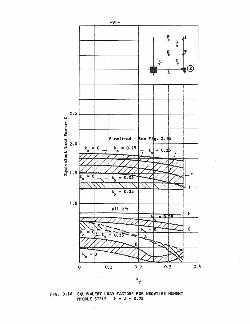
... 91 .....
I I ~ I
I G •
I E 1'1 , • ~ D •
..... -;0 A
I ! ! ~ t
2 .. 5
\
I I I
/
I I I I
I
I I
B omit ted - See Fi~ .. 3 .. 1 6 I "
~ I k lIIii 0 k IIiII 0 .. 15 7 k~ lIIIII 0 .. 2 x, --, x -7 I
V// / 1/ / / / / I / / / i
v// // [7// V// /
t?2 ~ '// /'~ V/ // / /L /// V// .,.. /
k ·R (J ~ k • p .. 3~ ~ 0 V>' f-f x x
~"" ,'" '" " ~""'" ~ "'" ~ "'" '" '" \,. '" "'" "- .,,~ • k = 0.35
I x
. I I
, .0 all k ·s I
It .. n ~c;, .~ H ./ / /
~~ 'I,r _ r x
M k I:
x
o
17// v//v/// ~ I
~c~ V7~
//// 7z7 ~--~ k I: ,~ 'v «? ...-.,.
}- kx = O.3sr---~
~ /7; 7/?~D ~ I
"""'-~,,,,,,,,~ I
~ ~ ~ ~ \
~ 0 ~
v-R 0.1 0.2
k Y
FIG .. 3.14 EQUIVAlENT LOAD FACTORS FOR NEGATIVE MOHENT HIDDLE STRIP . H = J = 0.25
E
0.4
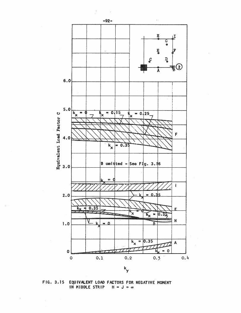
-92 ....
:g I G ED
E I~ ED
EDC D
ED
A ~~(!)
6 .. 0
5.0 k - ~ D I - O. x . 7 x .
.'" '" " " '" '\ '\ "'~ " ." "-'" '\ _"\.~
~ ~~ ~~~ " " '\ , k
x
B omit
II<. == ( A
~h W~ ~'l~ 2 .. 0
KW ,"" "" "" [\~~ k~ 8 0.35 1--.....
'Lie - 0 )C 1.,0
.. o F
o 0 .. 1
I ! I ;
j ! i l
15 I II1II 0 257 I 7 x
~~ " -~'<'~ '\ .~'\ ~
~~ ~ "'\ '\,~ ~ ~1F C\~
~~ ~~" "''''~ "'-.'\ _'\. 1'\ '~ -~ ~ - 0.3:
ted - See Fi g. 3.16 I I
VZh ~/ ~// W~ I
\-k - 0 ~ Is 1/ ~
~I ~~ ~ ~ I. ~"'~ F I"X - '"
k :: x
. .," -/ / tI' / V./~
0.2
k Y
r~- o~ - H n
I 0 .. 35
~ A
~ bt - 0
0.3
FIG. 3.15 EQUIVAlENT LOAD FACTORS FOR NEGATIVE MOMENT IN MIDDLE STRIP H - J = ~
0.4
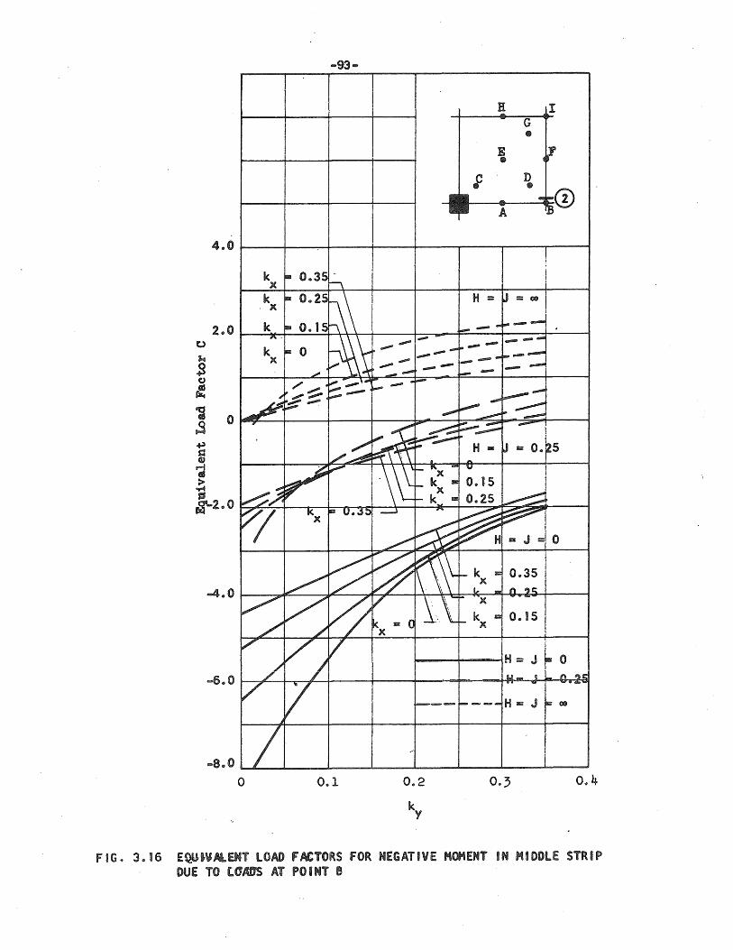
... 93 ...
H I
• E •
; D • A
4 .. 0
2 .. 0 t.> <fIIII1"'" -$.G .s (J
r:! 'i 0 .s ~ s::: ~ ., > "1"'4 S' $-2 .. 0
FIG~ 3 .. 16 E~~VAlENT lOAD FACTORS FOR NEGATIVE MOMENT IN MIDDLE STRIP DUE TO laADS AT POINT B
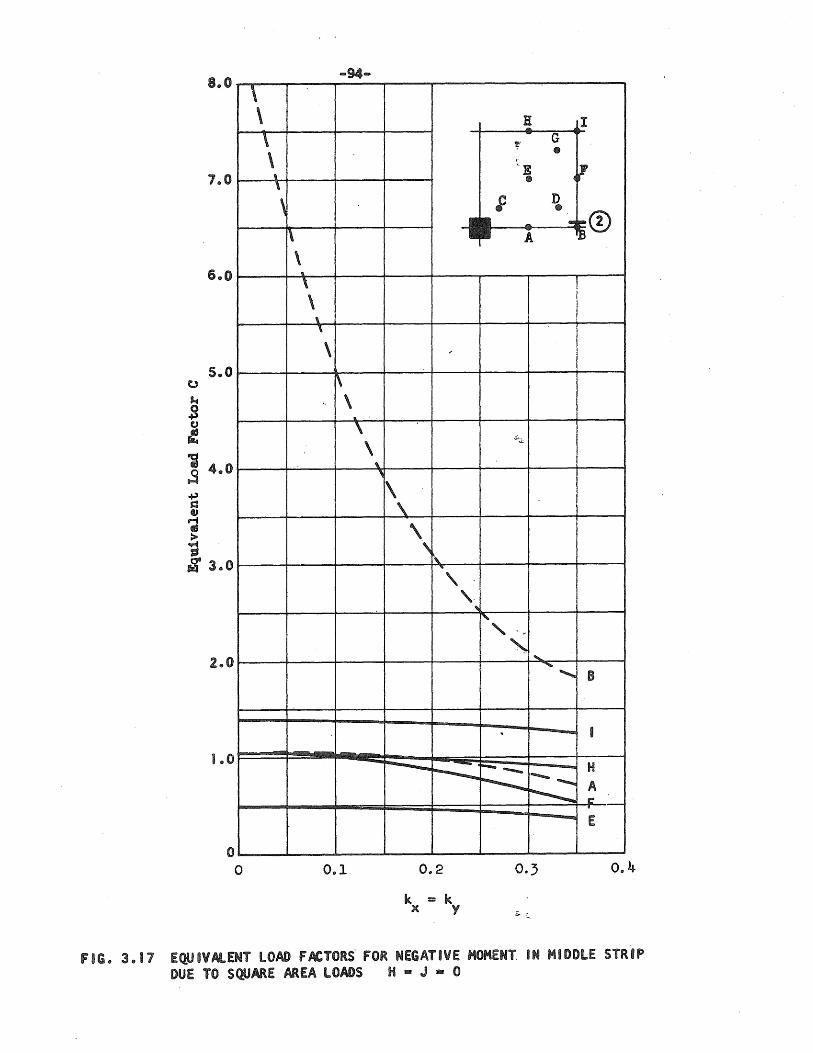
8.0 \ \ \ \ ,
'\ 1.0 , I' \
11
\
\ \. '\
s.o
1.0
o o
-94-
\
~ " \
.. \ \ " ,
-
0 .. 1
,
\ \
\ \~
... , " '"
r----:;.: ~
0 .. 2
k = k x y
~ I ~:
-G •
<E 4~ ti
~ D • ... mp ®
A 1}3
! I I
I I
¥4u..=
f' , .~ , ..... ' ........ B
, "- • H
I""""'- __ ....... ~ """'- .........
~ A IE' .
...... E
0 .. 4
fiG" l,,11 E~IVAlENT LOAD FACTORS' FOR NEGATIVE MOMENT IN MIDDLE STRIP DUE TO SQUARE AREA LOADS H - J - 0
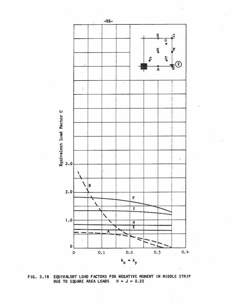
I II I .... G •
E dF •
; D • ~p.® I
A 1:8
. , ! .1
l
.1 i I ! ;
I I I
I ! I
I ! I I
I
\ I \
2 .. 0
..
I \ B ,
" f I '\ , --------- .......-. i \.. • -~ , "l
"- &.I I VI
1 .. 0 "Ill E .... -- - .......... i- A '-r- ......... ~~ .......,;; .................... ~ I ~ ......... . ~,...! o
o 0.1 0.2 0 .. 4
k - k x y
FIG~ 3 .. 18 E~8VALENT LOAD fACTORS FOR NEGATIVE MOMENT IN MIDDLE STRIP DUE TO SQUARE AREA LOADS H = J Il: 0 .. 25
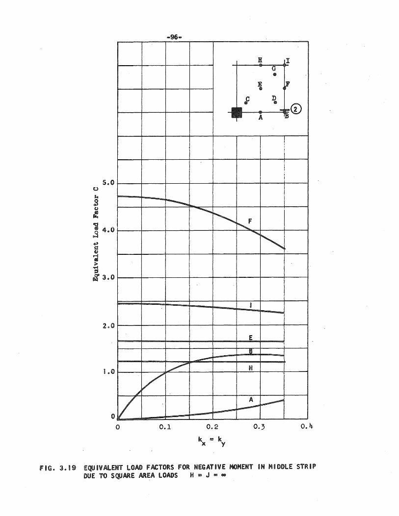
5.0
2 .. 0
B .. 0
./
o :/ o
~bm.
~
V
0 .. 1
~
'"
~-
0.2
k :::: k x y
:g I - G •
E ~ • f D • ~-[) .-
A ~
I !
I i ! I j
1
I l j
i
~ "'" I
• -E
8
H
A ~ ~
0.; 0 .. 4
fiG .. 3 .. 19 EQUIVAlENT LOAD fACTORS FOR NEGATIVE MOMENT IN MIDDLE STRIP DUE T'O S(JJARE AREA LOADS H:::: J &: 00
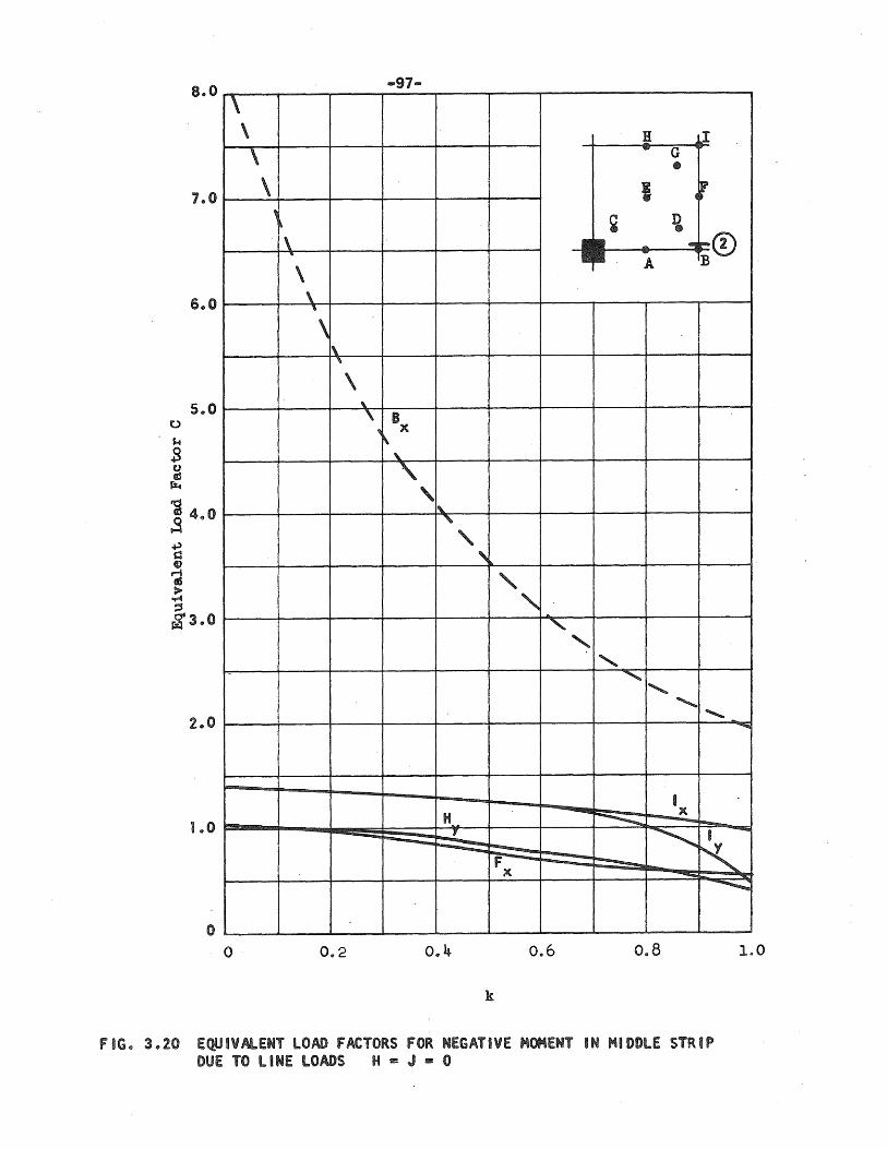
8.0 .... 97 ....
\ \ B II
\ ... G
• 7.0 \ I 4r ,
~ D , • . \ - ~~®
" --\
A IE
\ , 6 .. 0
\ i\
'\
\ '\
\ B 5 .. 0
\ x
\..
" , i,,-" " , ,
" " , "--
"" "-...........
.......... ..... 2 .. 0
I H~ ~
x --, ~ I -
---.;;: r;:::::::: ..
~ F -x
1.0
o o 0 .. 2 0 .. 4 0 .. 6 0.8 1.0
k
FIG .. 3 .. 20 E~IVALENT LOAD FACTORS FOR NEGATIVE MOMENT IN MIDDLE STRIP DUE TO LINE LOADS H = J - 0
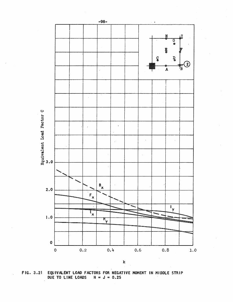
"
" " ~, ~
2 .. 0 ""'--
0.....- F ........ r----~ I x
1 .. 0
o o
i
B x !'o..,
... ~,
~ , .... .......... ~
My
0 .. 4
k
.... .......... """--
~ ~ -
1"\ c.. v.v
¥
..........
If II -- G •
I, cf D • '~~<Y -- IB A
! I
• Y ----r-----.
1'\ Q v.v
! '(
I ~ !
I
I
~ ...... -...............
"I 1"\ .L.v
fIG .. 3 .. 21 EQUIVALENT LOAD FACTORS FOR NEGATIVE MOMENT IN MIDDLE STRIP DUE TO LINE LOADS H = J a Oe2S

... 99 ... ·.
B LI lOU -G-
o
B. cf • ¥ D
0
~ .. (!) ~ .... A B
/
5 .. 0
~ "'-........
'" ~" " " s:
"""
'" '-I '" "-y "- ~
""""-~ ~ ~ I
~ ~ ~ ~
"-
2 .. 0
Ii ~ Y ~ ---- ---.. ~
1 .. 0
B • ~ for .11 k'~ x
o 0 .. 2 0.,4 0.6 0.8 1.0
k
fIG .. 3 .. 22 EQUIVAlENT LOAD fACTORS fOR NEGATIVE MOMENT IN MIDDLE STRIP DUE TO LINE LOADS Ii - J - ~
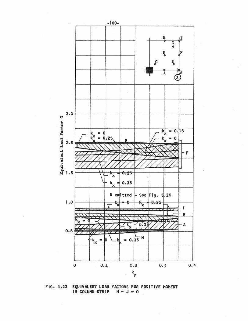
2 .. 5
1.0
0.5
... 100 ....
I
k • ( r kX == ( .02~ D x [)('... '\. '\. '\
~"''\ ~"'~ k\. "'" "" " ,~
",C;X ~ //// /// /
/// / /// /// /// // // / /// / / / / /
//// j/JY j//L V// 7~ \ \ . ..... .......
'\ r- .... x - ""'.o",oJ
f- k BI 0 .. 3'5 x
80R1 itted .... See I "" • r.- .... x "" "x
~'\.'\.. '\..'\..'\.. I, '\.. '\.. , '\. , '\. " " ~~( '7 ", "\. '\. '\. -<
V 7~-~ ~ O:3~ 17/// //)( / / / / / / 1/// / /
IL-v ~f-k := 0 k II: 0 ..
~ 135 H
x -
o 0.1 0.2
k Y
I:! I G •
E :F • .C D •
- f-
A -r~
I I ! • I j
I 1
! I ~
i \ I
I 1< Ix • 0·115 1;= ~ Pc == ~L
IV\ ~ ~
~x~ ~ -F 1/
C/~ ~ 1-j i
I Fig .. 3 .26 !
I
........... V .. .;;8..,
~ • ' I r- .... E
I"'\. "'\. " '\. ...... ~ A ~
~/j V~ f-A
0·3
FIG .. 3.23 EQUIVALENT LOAD FACTORS FOR POSITI_VE MOHENT IN COLUMN STRIP H = J == 0
0 .. 4
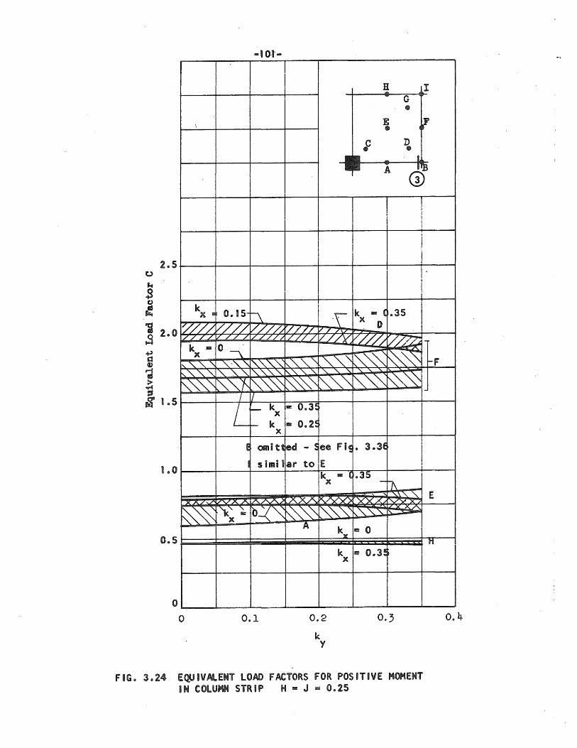
\
2 .. 5
kx :::: 0 .. 15-i.\ 777/ [.7/// ///// //// 17 / / / ./////
k = o . x \
I, " '" '\ ",'\. "- I'\.'\. '\.. '"
t-.. '\. '\. '\. '\. '\. '\. I'\...'\...'\...'
~"'''' '" ~"'" ~ ""~ I II .
L F-- k x r- k
x
E omitt
I simi 1
Y A/ .... / 7'VX A .A.AA~
~~ '''k~ ~ X ro0 0 .. 5
o o 0 .. 1
H I G •
E ~ • ; D •
- t A d)
I I ! i I I
I I I· I
I I
-\ k - ( .. 35
/'/// v / / ~ D /// / VT/57 ///// //LZ -
t\. '" '" "- '" "'-'\ ~~~ ~~ I-F t\.''\.. '\.. '\. '\. '\. " " "0~ ~"'~ "\ ~~"" ~~'" -1111: O.3~
- O.2~
ed .... S ee Fi~. 3 .. 3E !
ar to E k - ( x
AXA ~)
~~"\ ~"'~ A
0.2
k Y
kx
Ie. x
.35 11\ - -,\'\. , E
"'XXX ''v''Y"'5t
r--.""\. "\.. '\.. x/\.
III: 0 11
== O .. 3~
0·3
FIG .. 3.24 EQUIVALENT LOAD FACTORS FOR POSITIVE MOMENT IN COLUMN STRIP H· J = 0.25
0.4
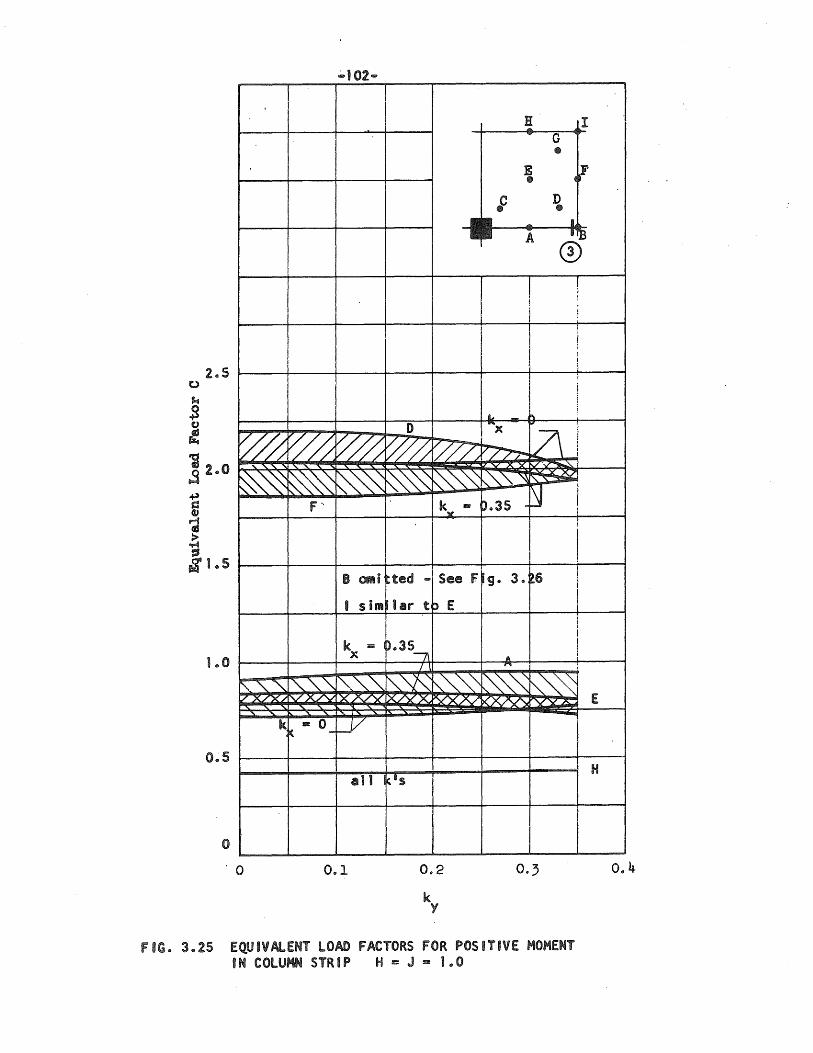
.;..'02 ....
I I
I
~ 'l~ ~ " '" '" , " ~~ ~~ ~~
F"
B ani
• s im
k = 1 .. 0
.x
r"-"-,," "'''''''' ~'\.'" [7 X/"X./ rvX/V x A/')(
k - 0 K -~
O~5
all
o '0 0 .. 1
D
~// //7 ~~ ~"'-~
k IIII! ·w
Ioted ... See F
Jar t J E
),,35/\ / \
~~ "",-"'0 D(/VX ~j<',/
<.'s
0.2
k Y
H I ... G •
E lr • .C D •
- I,
A 1''l3
® I J l I ,
j
I 1 I ; i
t. .... h ~
"'x
k7\1 ~ AX V'V"'!Io...."-. ~
,,",,, '" ~ ",~ N I p.35 I
i
I g. 3 .. ~6 !
I I
I J;, n
~~~ ~~~ b(~ VY2S. -
0·3
FIG. 3.25 EQUIVAlENT LOAD FACTORS FOR POSITIVE MOMENT IN COLUMN STRIP H = J = 1.0
E
H
0.4
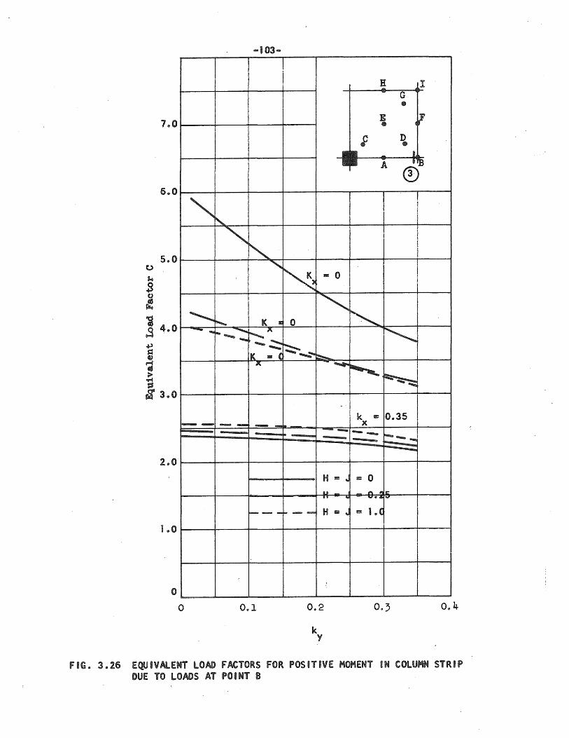
1.0
0,,0
" 5 .. 0
~ - ....
--2.0
1,,0
o o
.... 103 ...
I i
,
'" " "' ~ == 0
~ , I< a: 0 .................... ........... ~ ..... ....... .::::
II< B ( ........ ........:--~
x ......
..
- ........ .............. 1.. --- --H == qJ
u
" ...
---- -- ...... H m "
0 .. 1 0 .. 2
k Y
H I """
G •
E 4~ • f D •
.... I . A IB
® , I
1
I I !
i !
I
" ~ i
~ I
~
k = 0 .. 35 oX --............... t::.---
:"""""'" -=: ()
#\ "'E' ........ "'" =: I. (
0.3 0 .. 4
fIG. 3 .. 26 EQUIVAlENT LOAD FACTORS FOR POSITIVE MOMENT IN COLUMN STRIP DUE TO LOADS AT POINT B
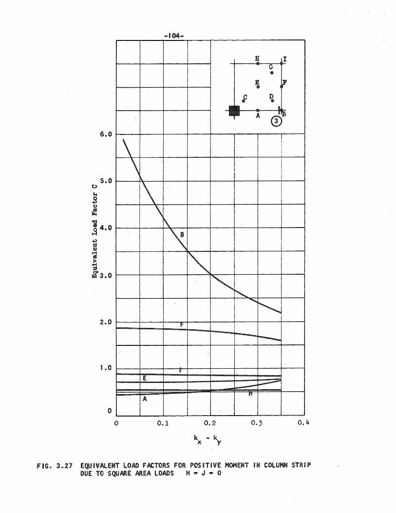
6.0
\ \
2.0
1.0
o o
... 104 ...
\
\ \
\
'\
f
I
E:
A
0 .. 1
I
~
'"
0.2
k - k x y
H I .... G •
E 4" (I
i D (I
t
A u'r:a CD
I ! !
~ ; 1
I !
1 ! ! I j
i I
I
I I I I ,
"-" ~l
--r---...-I
..-.-~
"
,0.4
FIG. 3.27 EQUIVAlENT LOAD FACTORS FOR POSITIVE MOHENT IN COLUMN STRIP DUE TO SQUARE AREA LOADS H =: J =: 0
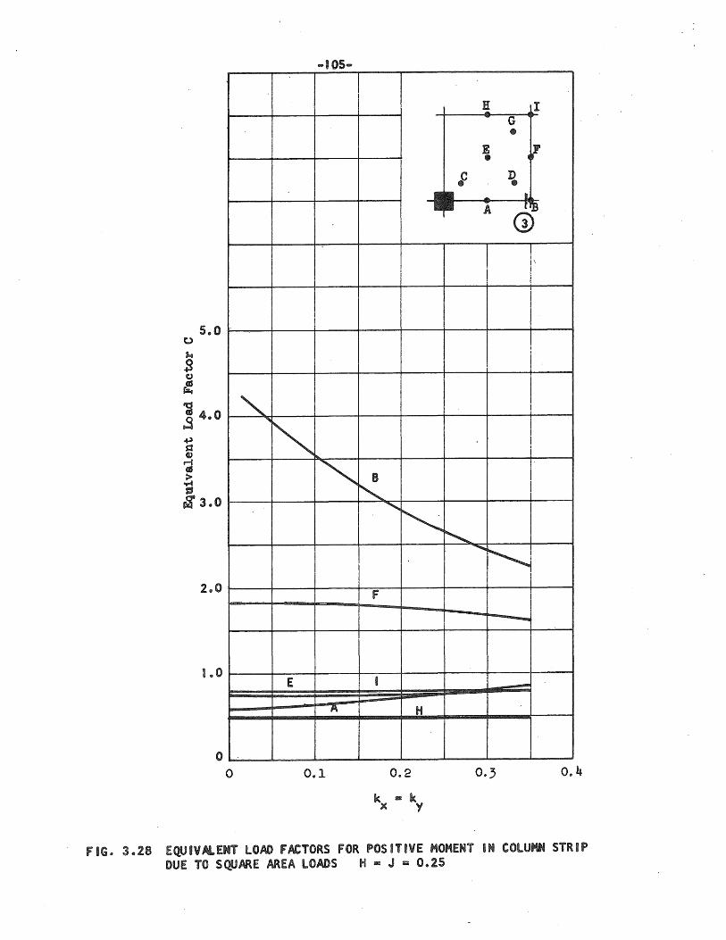
-105-
5.0
" ~~ ~
2 .. 0
1 .. 0 E
A
o 0 .. 1
I
B
'" " " F
I
H
0.2
k - k X Y
~ I ... G •
E ell • ~ D •
• A flB
G) I 1\
!
i
I
I
I i I
~ I ........ ~.
.........
-
0 .. 4
fiG. 3.28 EQUIVALENT LOAD fACTORS FOR POSITIVE MOMENT IN COLUMN STRIP DUE TO S QUARE AREA LOADS Ii == J :: 0.25
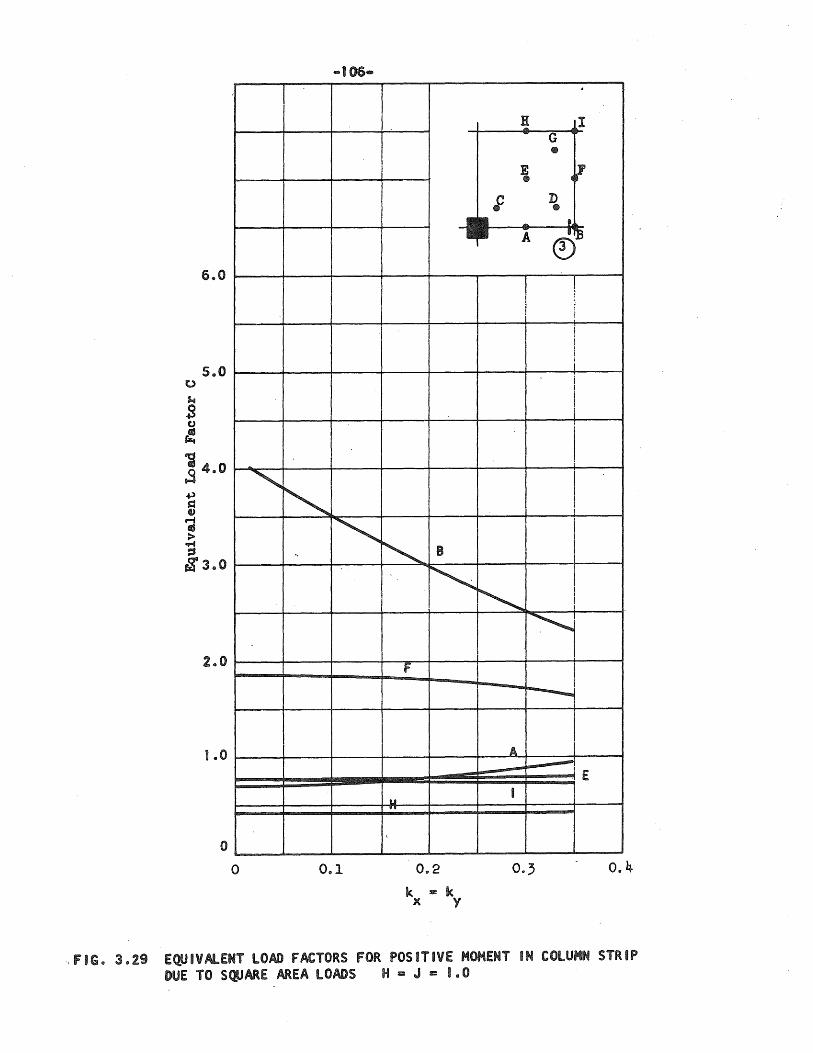
. l! I ~ -G
• E ~ •
~ D • II
A riJlll 6.0
! ~ I l I i
I I I i I
~ ~ I ~ ~ " S
.~
" I
~
2 .. 0 F
----........
A -1 .. 0 E
I IJI ..
I
o o 0,,1 0 .. 2 0 .. 3 0 .. 4
k - k x y
,FIG. 3.29 EQUIVAlENT lOAD FACTORS FOR POSITIVE MOMENT IN COLUMN STRIP DUE TO SQUARE AREA LOADS H:I J Ie 1.0
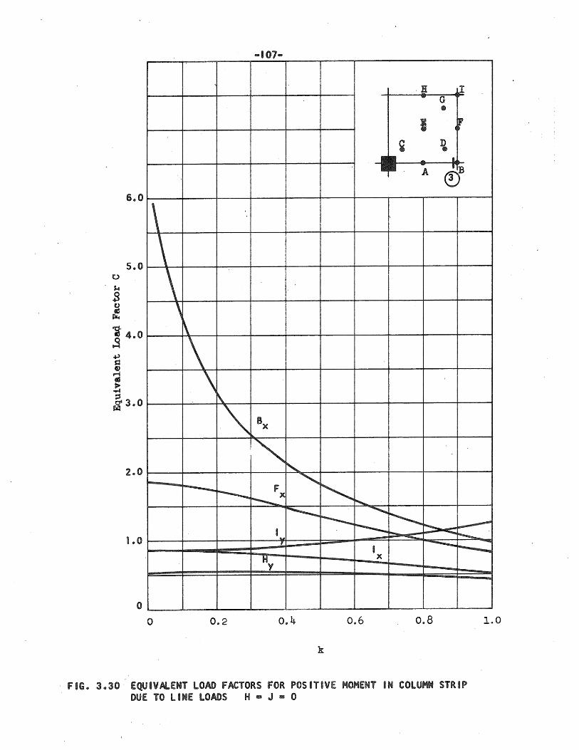
·Ii II """ G
• I 4r
¥ D • - L ....
ctB A
6.0
\ \ \
5.0
\ \
\ \ ~
.~ Bx
.", "-
~ "' - ----- Fx " --....--...... ~ ...........
2.0
~ ~
--........
~ ~ ~ I .. ~ , -I ~
. My X
1..0
o o 0.2 0,,4 0.6 0.8 1.0
k
. FIG. 3.30 EQUIVALENT LOAD FACTORS FOR POSITIVE MOMENT IN COLUMN STRIP DUE TO LINE LOADS H - J - 0
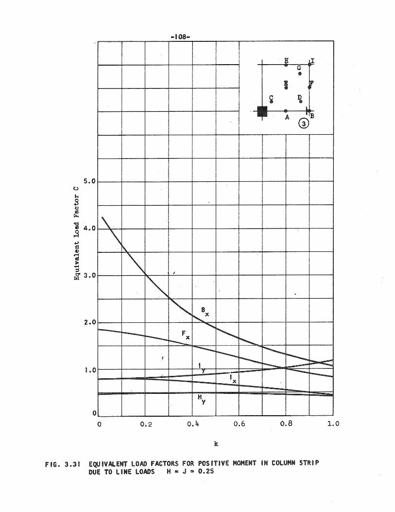
.... 108-
I 1I II - G •
E ~r • ¥ ~
- fa. .... filB A
@ i
I I
I _I
I i
5 .. 0 I
\-'\
.i\.
'\ I
; I
'" I I
" B ~x_
----- '" ~ r---.. F ----- x ~ ~
2 .. 0
............... ... ~ ~ e ~ ~~ -I ~ -
I
., ----r---.. I 1 .. 0
x
H y
o o 0.2 0 .. 4 0.6 0.8
k
FIG. 3.31 EQUIVAlENT LOAD FACTORS FOR POSITIVE HOHENT IN COLUMN STR-If DUE TO LINE lOADS H R J 3 0 .. 25
1.0
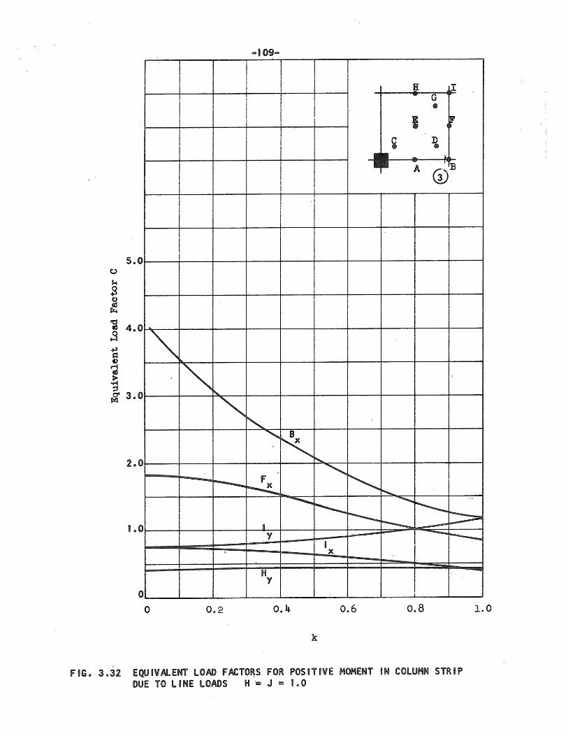
... 109 ....
{i ~I I
.... G , •
I r ¥ D •
- ~. - (i)IB A
I
5.0
~
'" "'~ ~ ~
"" . B
K-. .........
F "' '" --~ ~ ........
2.0
1 .. 0
~ ........... ~
-~ r----- ~
• ----... ------v ---. -----,. I
" x
H -Y
o o 0 .. 2 0 .. 4 0 .. 6 0 .. 8 1.0
k
FIG. 3.32 EQUIVALENT LOAD FACTO~S FOR POSITIVE MOMENT IN COLUMN STRIP DUE TO LINE LOADS H = J = 1.0
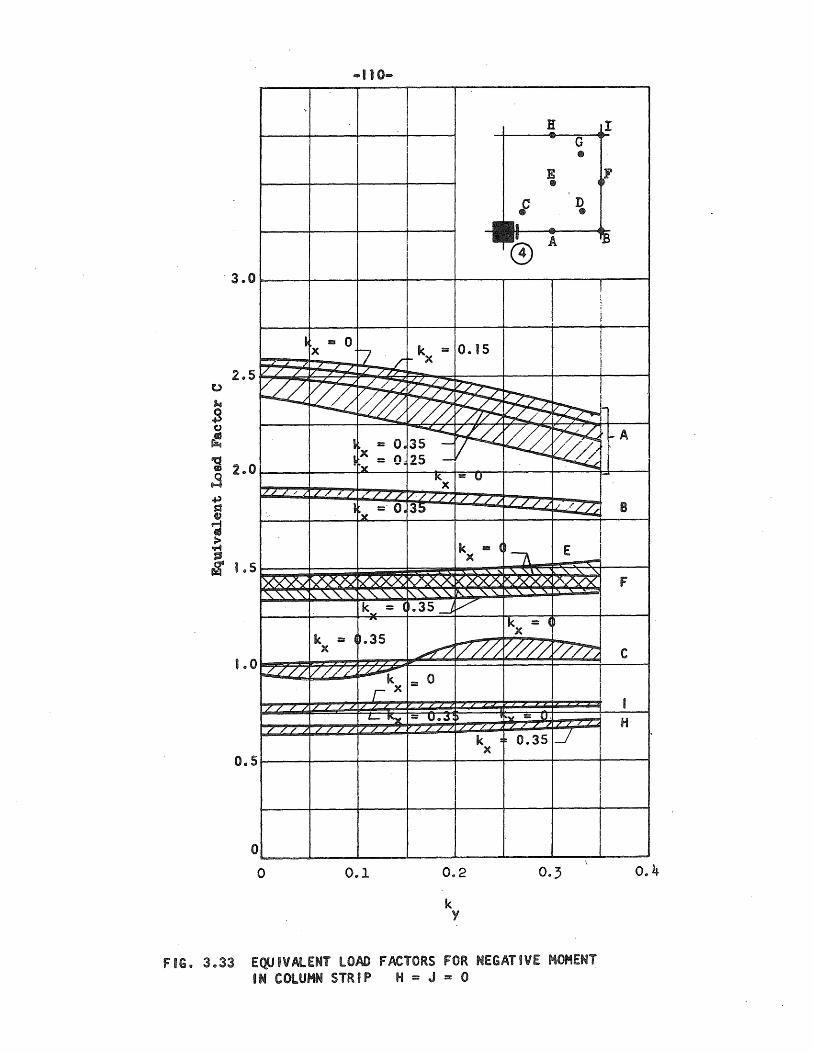
... 110 ....
" I H I ... G .,
E l~ ., f D .,
-0
A 1)
3.0 ! I
~ == 0 f- kx 0.15 I x 7 ==
!.......:: .L /" j IL' / / 7_ .L. 7'7"7-""-
~ ~ ~ ~ ~ ~ ! ~!-
2.5 0 ,.. 3
~ V4 ~ ~ r f- A
, z: 0.35 -0
&! ~r~ :: 0)25 -
. 1<x ::: U LLL/// / " ,; / //// V // / / ,/ / /
I ::- O. 35 //// ,'.,,"7'7; 1)( -
~ 2,,0 tD
3 ..., $:l ~
11 I k II1I:I ~ x 1\ E _I ~ ::s
~ I ,,5 '>6<:'X'V ,,-, "
1" 0 !.,LL/ /
/ / / /
/ / / ./
0 .. 5
o o
~ ~
'" '" k, = C ... ,
k =1 ~.35 x
//// v~ k ,-x
-,/
l-"'x ./ ./ ,/ ./ ////
0.1
""'" '<."N\X KXXA K/XX;X
" "" 1/'1..." ,,"- ""'" .35~ V
k =~ x
~ t77'// V/// = 0
- u.-,) 'i"v - U. ./ ./ ,/7 ././ 7/
k x
0.2
k Y
/
: 0.35
" " " V\A/X
V777;
./~L
1-1'
FIG. 3 .. 33 EQUIVALENT LOAD FACTORS FOR NEGATIVE HOMENT IN COLUMN STRIP H = J :: 0
I
,
B
F
c
I H
0 .. 4
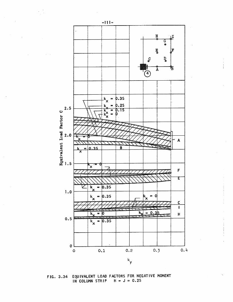
-'II ....
! I ! j H 'I i .... I G
• E , •
I .C D
I • I. -Ie A 113
~
I ! ; ,
I I
k := p.35 I \\
x l
k - 0.25 !' ...... ! ,
!\\\\ k - D.15 ! kX _ 0 I .......... x I j /./
/1 V'VVV' ..,...,......,.
I..LL / A/\/
~ ~ ~ I
~ ~ ~ ~ • ru -.....-. "'x .... ~ ~/ 20 ~ .... A
" """ i' "\. "\. "\. '\ "" ,,~ Ie. II:
x '
V/// \
~ 1.0
0.5
o o
~
77/ '///
0.35
-"'x ..... '" ~
1/// / '// V/
~"'~ ~"'~ k II:
x P.35
k -0.35 x
V// /7// ///-J/ V77/
ky = ~ k • 0.35 x
'" " "', -, B
1//// '/// '\.
~~~ ~ """ ~
/// :/I/V/ v / ./
'\.
kx
0.2
k Y
1', """~ ....
! ~
I
'/// -/ /L£. I'\."'\. '\.. """"-'. ~'" " "- ,,"\:S'l
k. == (J X
V/ // /777 /
' "-..;;:
= 0.315 !
FIG. 3.34 EQUIVALENT LOAD FACTORS FOR NEGATIVE MOMENT IN COLUMN STRIP H = J = 0.25
F
f
C i
H
0.4
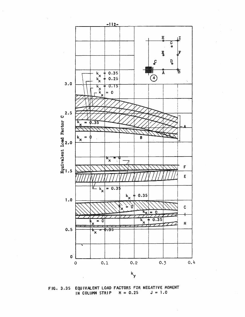
-112 ....
I I H .... I G •
E JF • .C D
I • -
3 .. 0 \r f- k : 0,,35 A 13
x 0 k I 0.25 ~ x
\ b- k : ~ O.I!>
I I x ~ 1\ r k = 0 I
V//\./\ y~ ....
822-' 1/~ ~ ~~ ~/'V /// /// ~ 17 / / / ./ 7
~/'J/ V// ~ ~ ~ ~ ~-k = ~.35 ;.4 X
" " " " " '" '\ """""" k = ~ . x
K -, x ,
~~~ ~~" ~~"" 'III I Jill I, rrl I I
/ iLk
x = O .. 3~
~ ~ ~~ / / / / / / 1/ / /
r". lIE': 0 x . ....,.. .... , ... II·~-.I
X 0 .. 5
"
o 0,,1
~ "'-""~ --i\..".~_"\ 8
~
11 ~~' ~"'''' "'-III I / rill
kx ~ 0.35
~ "'="') ~ x~ 1<)(
/ / / / / /
kx
0.2
k Y
/// V// ~'" '\:~ ~Xj
!-
! I 1 I
Ii\.. " " '" ~ '" "'" I fill ///1
I
1 ~~ ~
lIE': 0 --/ / / ./ L ~
I\: 0 .. 35 ./ ./ /.ZL
I
I
0.3
FIG. 3.35 EQUIVAlENT LOAD FAC~ORS FOR NEGATIVE MOMENT IN COLUMN STRIP H = O.2~ J = 1.0
F
E
C ~
T
H
0,,4
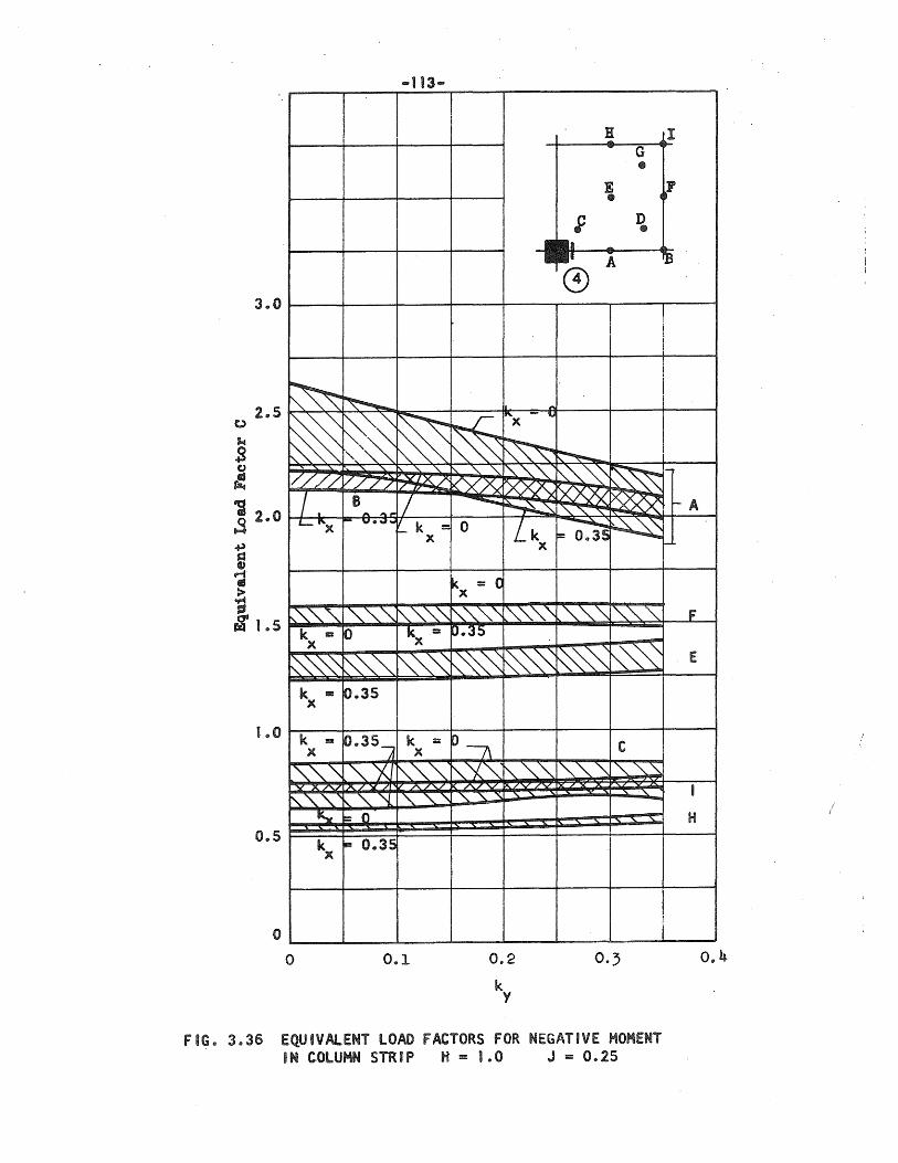
B I .... G •
E ~lr "
3 .. 0
~ ~
~ ~~ ~ "~'~~
2.5
" " " ~ //// V7"/7' ~
I . B / ,.. ... ,.. L- "x v.~ ...
I k = - x
~"''' "''''~ '" '" "''' k :: ~ k, .= x oX
~~ ~'" '" ~"'~ k - 0.35 x
k = O .. 35~ k = x x
1..0
~" "')( ,,'" '" 'V X7'\.] -x X/ /'-./"./
~"\."\. I\. "\. "4 " '" " ~ = 0 0 .. 5
kX !l: 0.35
o o 0 .. 1
I. "
~ I"X - ..
~ I\. " " "'''~ b()()\( ~ .............. ~
0 Lk x
~. = C x ~,,~ ~'" " 0 .. 35
&~ ~~
p/\
" "'i"-" "<', /'-/ '-/ D\../V ,,~ "
0 .. 2
k Y
i D •
(3) A
~
~~~ ~ rxm ~ ,,'- " ~ ~ 0 .. 35 ~
""" '" '" '" ~""~ ~
C
"'''''''' ,,~ " -'-.
I
0.:;
FIG. 3 .. 36 EQUIVALENT LOAD FACTORS FOR NEGATIVE HOME NT IN COLUMN STRIP H = 1 .. 0 J = 0.25
1]3.
, I I
I I I I
1-
-A
I-
F
E
I
H
j
0 .. 4
/ I
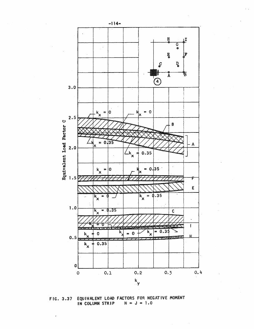
-ll4 ...
3 .. 0
~k = 0 r x
~ V// ~ ~ l?<X.X k'~
2 .. 5
x 'X ,]A .L / . 1/ / /
L, -~~ , == OC x
k ZIt 0 x
777 / / / 7
/ / // V / /, V !/7 / /
~~ ~~ ~ - k == ( -J
x
k. ==. C .. 35 x 1 .. 0
~/~ o/~ ~~ 1// "'J =·u 1\77
k = 0 k) x 0 .. 5
k l ~ 0.35 x
o o 0.1
j
I
;-~ = 0 X
v E77 ~ IX"'''' ~ EZ)0
~ ~ ILk : -0.35 x
r· == 0. X
/1/ / '/ '7
/vvv /v/
~~~ ~~ k = ( x
V7h V// /// / / /
= 0 . Vk x
0 .. 2
k .y
~ I "" G
• E c,
CD
~ D CD
II .... II A ~
0 ! ! I i
I I
.j \ !
I' ~_f B
I
~ ~ tA V// ~ ~ .J
35 .
/ //. //// r
~ ~'" ~~ E
.35
C I
V/~ ~ / / / / / '2.
I " == O.3~
- 104
0.;
FIG. 3 .. 37 EQUIVAlENT LOAD FACTORS FOR NEGATIVE MOMENT IN COLUMN STRIP H = J = 1.0
0 .. 4
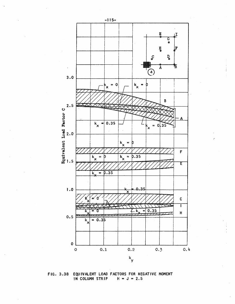
-115 ...
H I .... G •
E E' •
3 .. 0
2 .. 5
1 ., 0
0 .. 5
o
.C D • ...
8) A
I k. - 0 I
k - 0 x x /// / 1/ / 7 .,. -~ ~ ~ ~ ~ ~ ~ B :.....:::.....L<..~
~///
~
We( / /. X !'S:~A
kx
k x
o
A.. /'-./ ./ 'J' ....... 'it'
~
~ ~ ~ ~ k = 0 .. 35 x
v/// //// k = 0 x
~ ~ k = ..... 0.35
//c(/ ~ -z x7\A /\1K X
== 0
= 0 .. 35
0 .. 1
:(.0 ....J L -~
I k. = 0 x -
I . I
k :: 0 X
V// //// /// V/// k :: () .35 x -/ ~ W~ rm Y/LL
I
.l,. '" n "lC:; x
~ m ~ ~~l ",\'\\. ,\. \.'\ \.\.,\, \.~~
~_ ky :: 0.35 1-
I I
0.2
k Y
I I
FIG .. 3 .. 38 EQUIVAlENT LOAD FACTORS FOR NEGATIVE HOMENT IN COLUMN STRIP H - J = 2.5
:a
! j ; )
\
-A
F
E
C
I
H
/'
0 .. 4
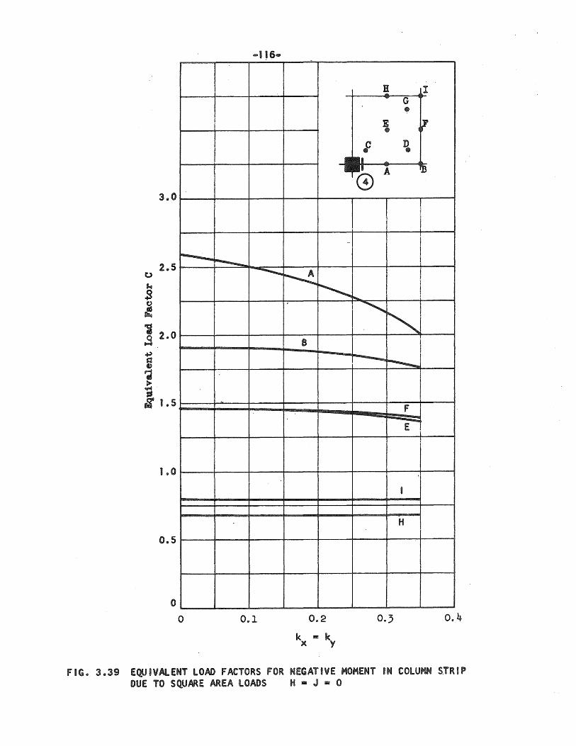
.... 116· , .
3.0
r-----~ ............... 2.5
t .. 0
0 .. 5
o o 0 .. 1
-
~ ~
8
0.2
k =: k x y
Ii I ... G
EIJ&
E ~ • ~ D •
....
8) A 13
! r
I I I I I
~ ! , " i --....... hJ
I F
E.
I
H
0.4
FIG. 3.39 EQUIVALENT LOAD FACTORS FOR NEGATIVE MOMENT IN COLUMN S,TRIP DUE TO SQUARE AREA LOADS H a J == 0
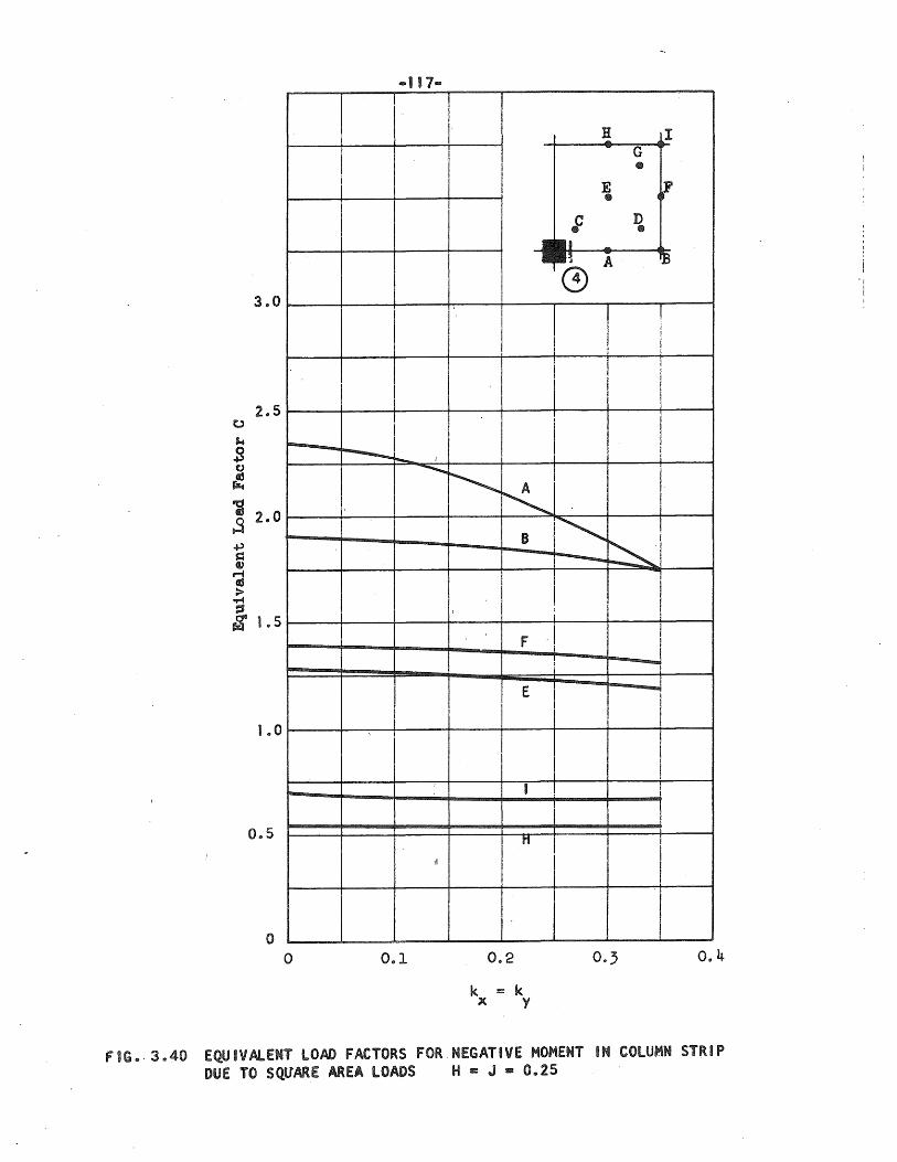
i
3.0
2.5
---- r----1-0....
i-
I...
1 .. 0
......
0 .. 5
o o 0 .. 1
I
..........
!
I
I ! I I
I
~ K S
F
E
I
Ii
0.2
k = k x y
H I .... G •
)' E (I
; D • II -I~ A ~
(9
! I i
! ! i i
I
! 1
I ! I
I
I~ I
~J --- l I !
I I
1 ~
I !
I
i
I
0.4
FIG •. 3.40 EQUIVAlENT LOAD FACTORS FOR NEGATIVE MOMENT IN COLUMN STRIP DUE TO SQUARE AREA LOADS H II:: J B 0.25
'j
I I

t,)
~ .s CJ
r:! i .s ..., s= OJ
~ > ..... s:s $
3.0
~
2.5
2.0
1.5
1.0
0.5
o o
; )
~ ~
I
./
0 .. 1
A ~
B
F
.. ~
• H
~
..--..,
0 .. 2
k := k x y
H I ... G •
E ~ • ~ D
' . .... A ~
0 , , i
i I !
" ,
-.............. ~ t
I !
...........
-
I
0., 0.4
FIG .. 3.41 EQUIVALENT' LOAD FACTORS FOR NEGATIVE MOMENT IN COLUMN STRIP DUE TO SQUARE MEA LO~S H :II: 0 .. 25 J - 1" ()
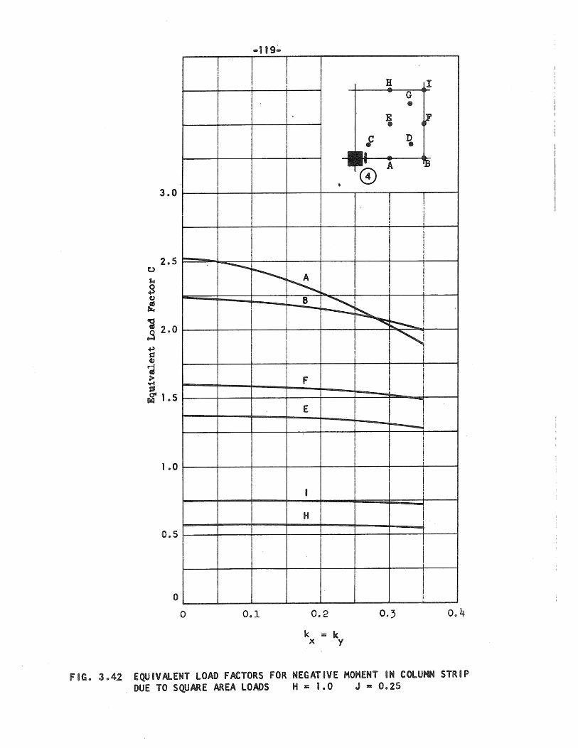
-lt9;"
! I I I f! I i
I I G
I •
! I I • E
4" !
I •
f D • II -"
A 13
0 • 3 .. 0
I 1
!
I ~
-- -........;..,.. ~
I I
K~ ! I
2 .. 5
B ~ I - ~ I -~ ~l
~ !
F ! I
E l --J
1
I I
• I I
1 .. 0
H
I i
I
0 .. 5
I ! o
° 0 .. 1 0.2 0 .. 4
k = k x y
FIG .. 3.42 EQUIVALENT LOAD FACTORS FOR NEGATIVE MOMENT IN COLUMN STRIP . DUE TO SQUARE AREA LOADS H 2C 1 .. 0 J :B 0 .. 25
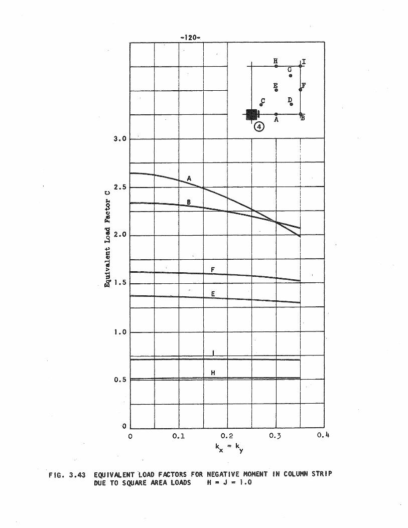
~ I - G .. E ~ ..
; D .. -A ~
@ 3 .. 0 !
!
1
I........
-~ ~
'" '" B ~
2 .. 5
--............ ~ i
~ I I
I
F I I ---/
- E
1 .. 0
I I
H 0.5
I
o 0 .. 1 0 .. 2 0., 0.4 k :: k x y
FIG. 3.43 EQUIVAlENT -LOAD FACTORS FOR NEGATIVE MOHENT IN COLUMN STRIP DUE TO SQUARE AREA LOADS H III J :: 1 .. 0
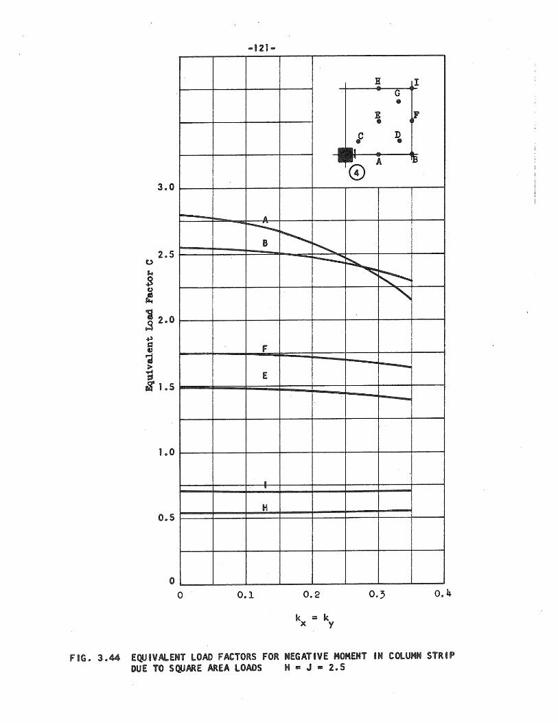
I l! I - G •
E JF • f D •
0 A ~
3.0 ! I
..... A I
-~ 1
~ I
B ~ I - r---.::: ~ ~
2.5
I " F I
-' E
-
L,O
D i u
H -,
0 .. 5
o o 0 .. 1 0.2 0 .. 4
k ::: k x y
FIGo 3044 EQUIVALENT LOAD FACTORS FOR NEGATIVE MOMENT IN COLUMN STRIP DUE TO SQUARE AREA LOADS H z: J z 2 .. 5
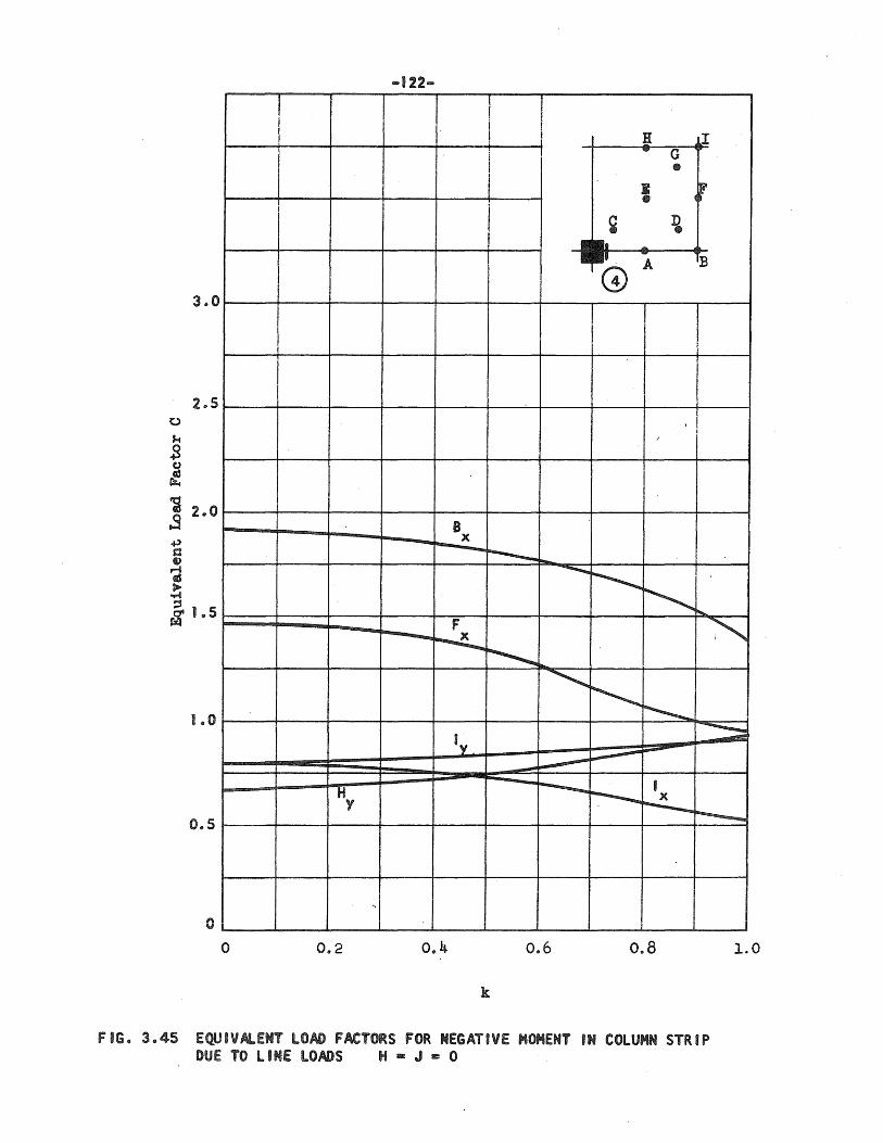
-122-
i I I ! H LI .... G ..
I r e·
i ¥ D .. -
. A G)
IB
3 .. 0
I I
2 .. 5 . ,
I I
B x - r----. - ..............,
~ ~
""'" F ~ ............ ~ ~ ~ ~ ~
Iy --::::;
~ ~ ---~ 1.,0
H --....... ~
I Y ~ r----. 0 .. 5
o~1 ~~~·~'I~·I __ ~~~~~~ o 0 .. 2 0 .. 4 0 .. 6 0.8 1.0
k
fIG. 3 .. 45 EQUIVALENT LOAD fACTORS FOR NEGATIVE MOMENT IN COLUMN STRIP DUE TO LINE LOADS H - J - 0
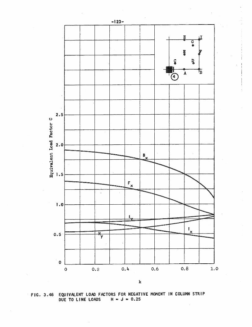
... 123-
T ! ~ II T ... G I
I •
i 4' !
• ¥ D I •
II -rJ ..." TB (£) A
2.5 I
- r----~ Bv -.............. ~ ~
f '" " ~ ~ ....... ~ " -
~ ~ ~ ~
1... ::::;;;...-
1.0
~ ~ --0 .. 5'
--.... ~ I
u i--.. x y ........... r----...
o I
o 0.2 0 .. 4 0 .. 6 0 .. 8 1.0
k
, FIG. 3 .. 46 EQUIVAlENT LOAD fACTORS fOR NEGATIVE MOMENT IN COLUMN STRIP DUE TO LINE LOADS H = J • 0.25
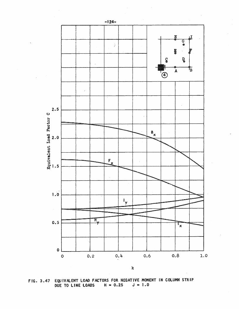
-124 ....
I ~. LI ".,
G • I
I 4f. ¥ ~
..... 1'1
A IB @)
2.5
I......
---r----. ~ ~ B
~x
~
" "'" ~ " '" ---........ ~ '" ~
~ ~ ~ ~
~ 1 .. 0
By -~ ~ = ..........",..
l----""'" -loom.... ----r----H .... r---... "'"---, IX r----... 0.5
o o 0.2 0 .. 4 0.6 0.8 1.0
k
FIG .. 3.47 EQUIVAlENT LOAD FACTORS FOR NEGATIVE MOMENT IN COLUMN STRIP DUE TO LINE LOADS H - 0.25 J z 1 .. 0
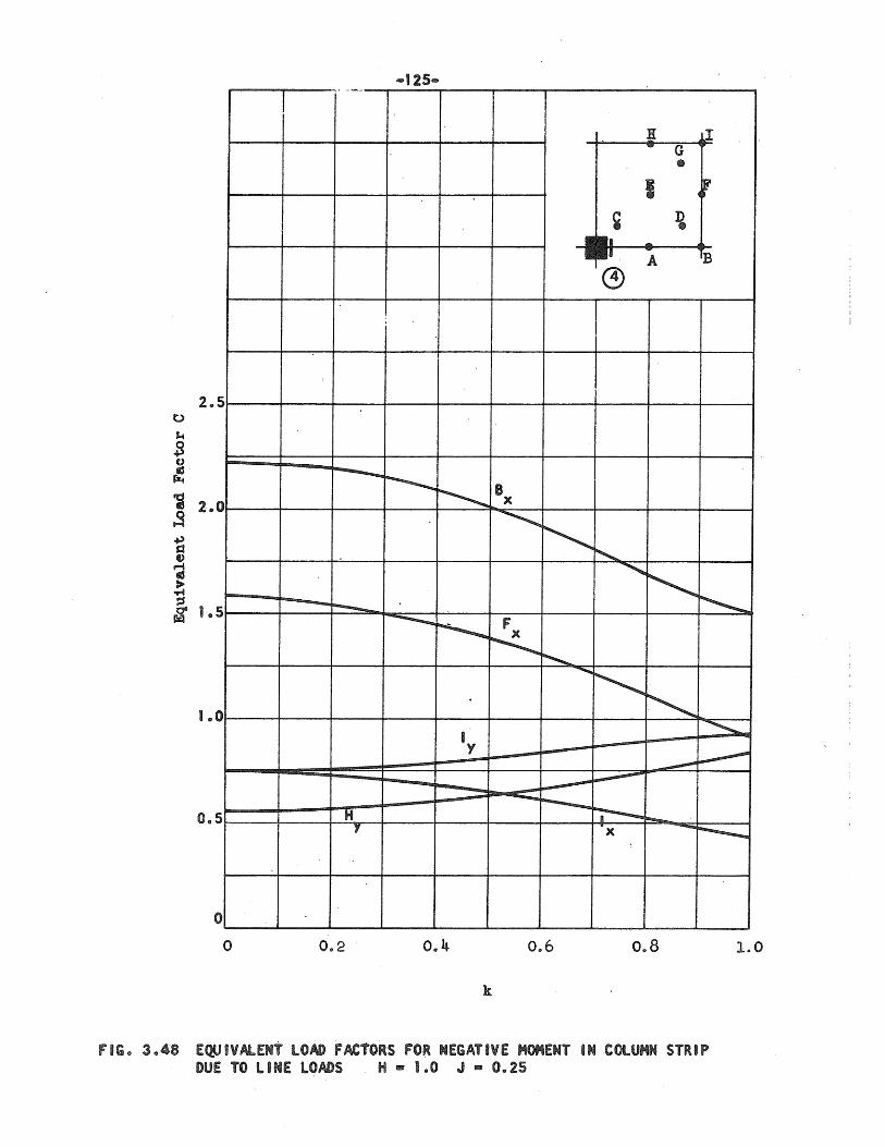
.... ~ ---'
II LI - G •
I cr ~ D • --
A IB
@
I
2 .. 5 0
~ .s C)
~ iJ 2 .. 0 3 +' d G>
-----~ ~ 8 x ~
" " M IS ~ ::::s oc 1.5 ~
'"' " ~ - r---. --............. ~
F
~ ~
1 .. 0
.........
~
" I ~ Y
~ .-..--
------------.... -----Ii ""l---~ y x ------
0 .. 5
l
I
o o 0 .. 2 0 .. 4 0 .. 6 0 .. 8 1.0
k
fiG .. 3.48 E~.VALENt lOAD FACTORS FOR NEGATIVE HOMENT IN COLUMN STRIP DUE TO lINE lOADS H - 1 .. 0 J B 0.25
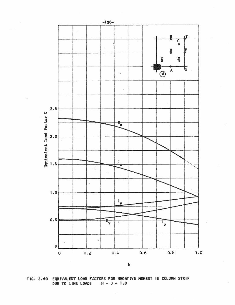
-126 ....
tI II ... G
~ • I· cf
¥ D • -
(9 A B
"
2 .. 5 ,
!.....-
............... 51
~ .... x ~ ~ ~
'" I I
~ -r---- f ~ ..... " - ............
~ ,~
. , .......
~ ~
........
~ ~ ~
J ,,0
Iy -..------~ ---
.......-."".. -~ - ---r----. til "'"'--fiy • ~Imo..
.• -X ---
0 .. 5
"
o o 0 .. 2 0,,4 0.6 0.8 1.0
k
fiG .. 3.49 EQUIVALENT LOAD fACTORS FOR NEGATIVE MOMENT IN COLUMN STRIP DUE TO LINE LOADS H • J ~ 1.0
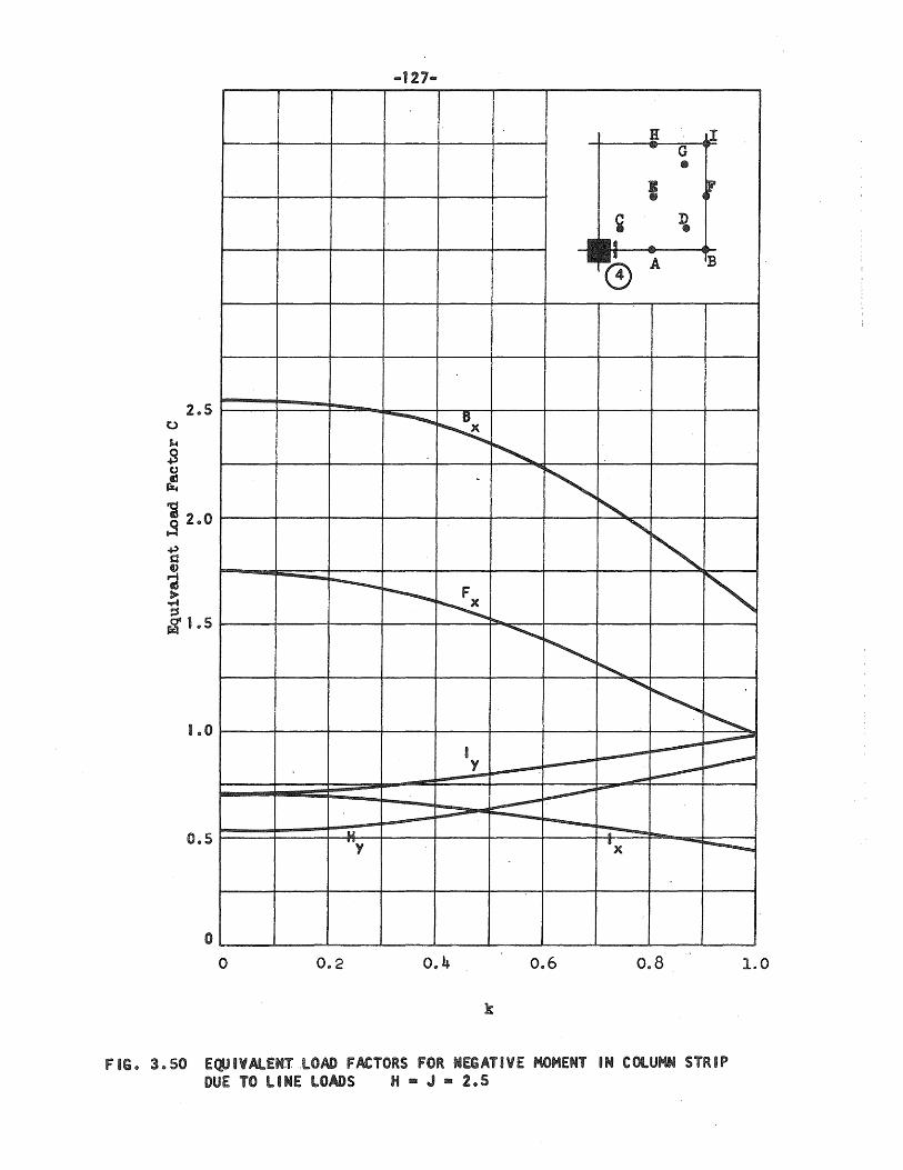
I I I' ~ LI
! - G •
B r .. ¥ D •
it .... J - IB
C9 A
2.5 ~ K
'-~
~" "'-" "'" r----
~ F
~- " "" " ~ ~ " ~ I ------------Y ----~ ~ ---~ 1.0
------........
----------~"'" lUI a -
...... .'y IIX -r---... 0.5
o o 0 .. 2 0 .. 4 0 .. 6 0.8 1.0
k
FIG. 3.50 EQUIVAlENT LOAD FACTORS FOR NEGATIVE MOMENT IN COLUMN STRIP DUE TO LINE LOADS H - J - 2.5
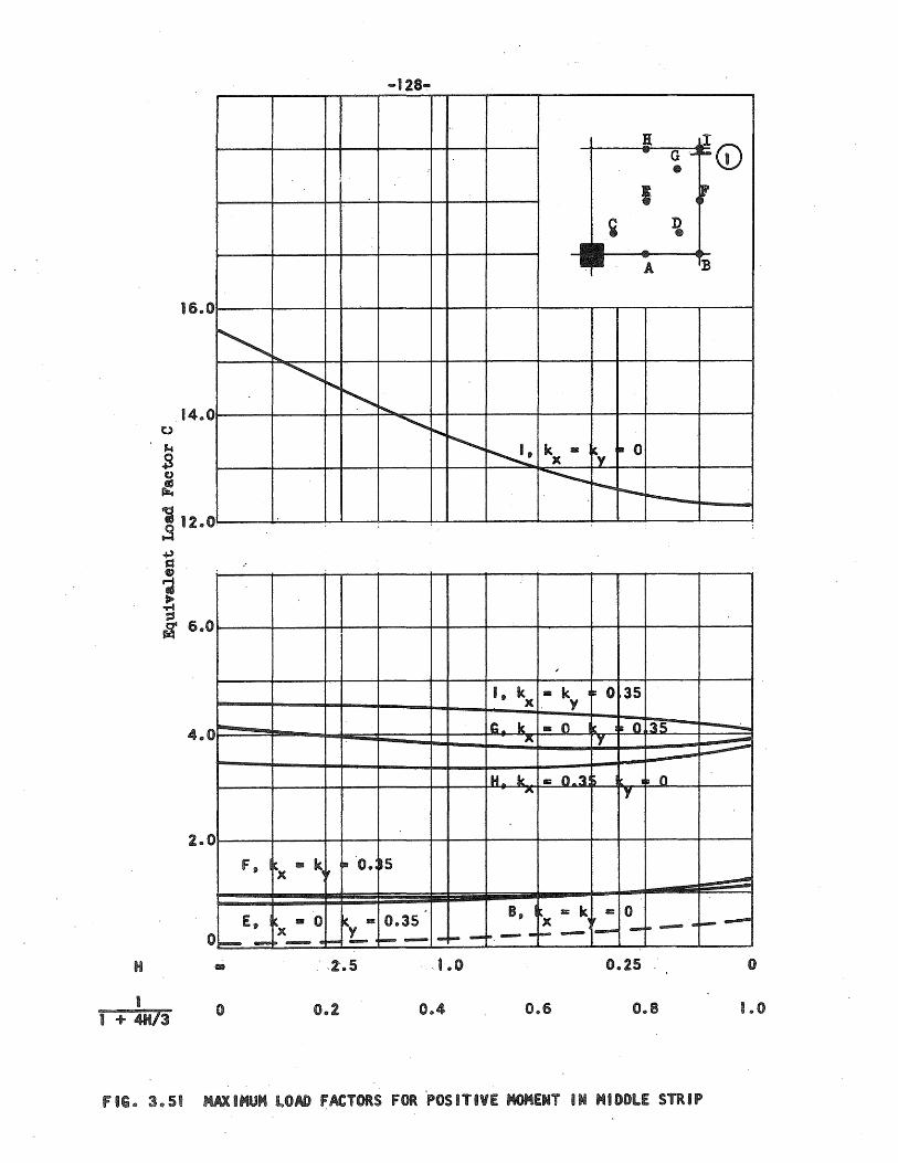
o·
Il II ... ~ '~~G) ;
:
I f ¥ D ..
-"" TB A
lS.0
"', 14.0
~ .........
~ "-~
~ ~ ~ k - fy -0
x ~ r---. ............. """"'--
,
I, k - k
~ 0 35 x o y
- G Ie. lillIE 0 It III 0 ,35 .......... oX Y --~ 4.0
H. Ie. II: 0 ~,1lI III 0 A J
2 .. 0
F8 ~. lillIE k x -~ If 1m '0. .5 -
E~ 1'. • 0 0 .. 35 B, I ~. - k = 0
K. = x ..-",,-'" i-- --x L- is. - - -- ---- ......... _ ..
I-- ~ ............ ---o Ii 1 .. 0 0 .. 25 o
1 + 411/3 0.2 0 .. 4 O .. S 0 .. 8 1..0
IMUHlOAD fACTORS FOR POSITIVE MOMENT IN MIDDLE STRIP
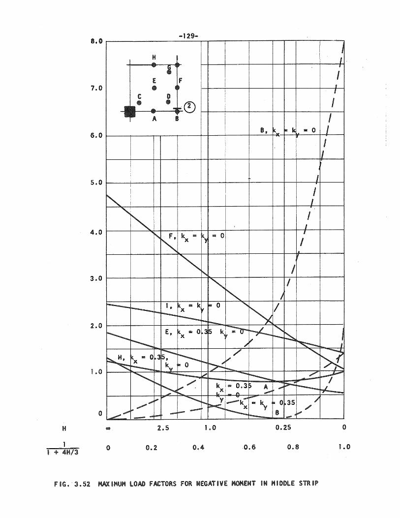
8.0 ... 129 ...
J H I ..... ..
i , I E F
7.0 • 0 , I
C I)
• • ..~® I -...... A I I
BIP ~- 1= Ie .." :lIZ 0 I j1 6 .. 0
I II
I " 5.0
~ I I
" " ,
'" I
I
~ 'Z k - 1<.)' - 0 I
X I II
4.0
~ 'I
~ /
'" I
'" I
3 .. 0
r----. ----.. I ~ k, - k V lIB 0 '" i'x / --r--... x
-----F- ......-...
~ E, k.. IE: 0 .. 3 5 k, ~ ~ " ~ J x """'-
~ / ~ ~ I
2.0
~ k.. == 0 .3 ~ ~
/ " >l x ky ..... r>:: ~ r--....- ~
'" ........ I---.. l/ -....
~ ~ ~ ~ /' ~ ~ ~ . k ID O.3p A po .,p ~ ~ I~X filii""'" ~ - 1'\ ' """"'-
1 • 0
'" "'" ~ "''1 ""-:k-.,..".....
/ ",.' I""-- - k 1= 0 1>35
~---><... ~
y " ~~ 100- - B ~ --- --- ~" o
2.5 1 .. 0 0 .. 25 o
1 + 4H/3 o 0 .. 2 0 .. 4 .0.6 0 .. 8 1 .. 0
FIG.·3.52 MAXIMUM LOAD FACTORS FOR NEGATIVE MOMENT iN MIDDLE STRIP
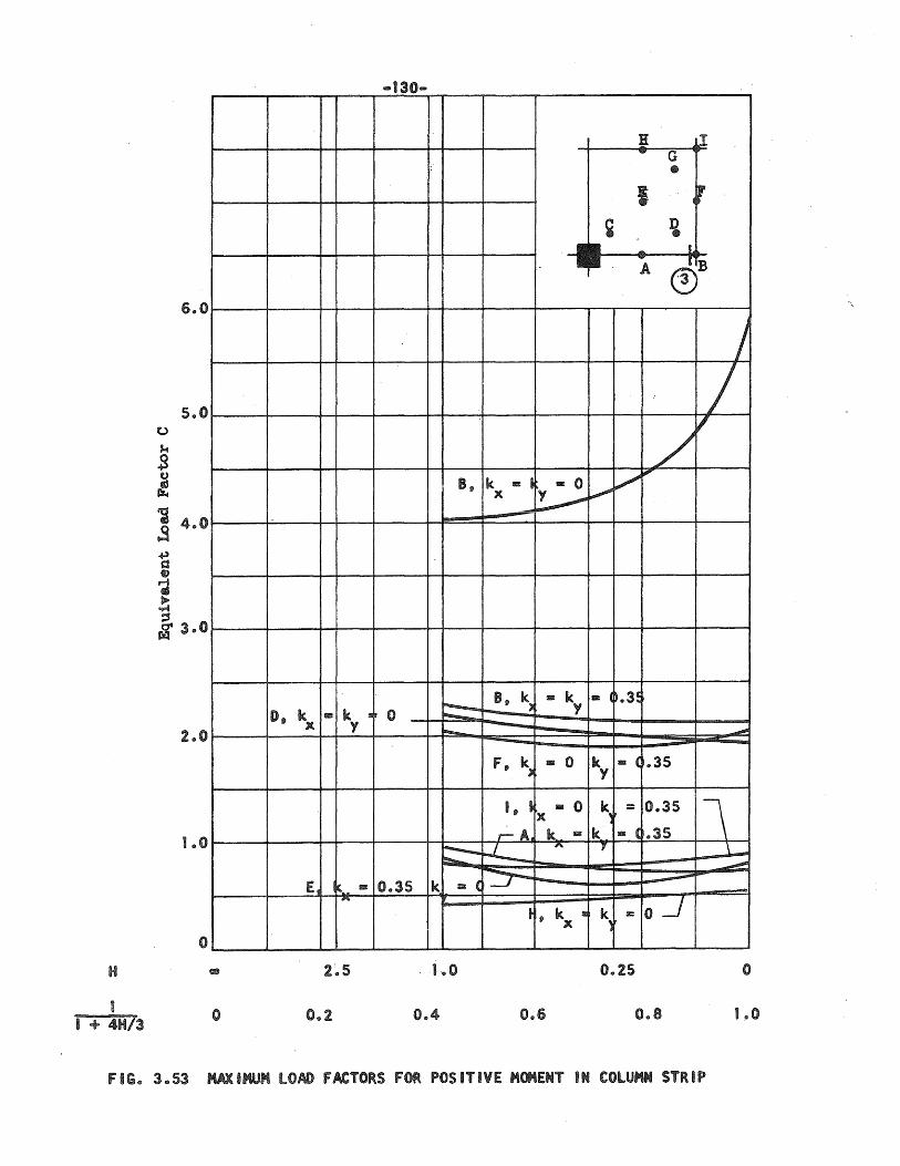
-130 ....
l! II .... G : •
I r • II
- J. "'" rff A
s.o
J /
/ v 5.0
B, k =: I llIII: 0 / ."
X ~ ~ -
~ B. k) • k .~ .3~
D. k • k :i 0 Y x y
~ ...-2.0
F fII k) lID 0 ky lID ( .. 35
1.0
I fII I lID 0 k~ =: 0 .. 35 \ x ":-14. k == k == ( .. 35
t:-~ ,.. ., L ....
~
E ~~ SIll 0.35 k SIll ( ~-- ~I""
..... O~ •• k :III k, :=
x o
Ii 2' .. 5 ·)...0 0.25 o
• + 4"/3 o 0.2 0 .. 4 0.6 0 .. 8 1 .. 0
fiG. 3.53 MAXIMUM lOAD FACTORS FOR POSITIVE MOMENT IN COLUM" STRIP
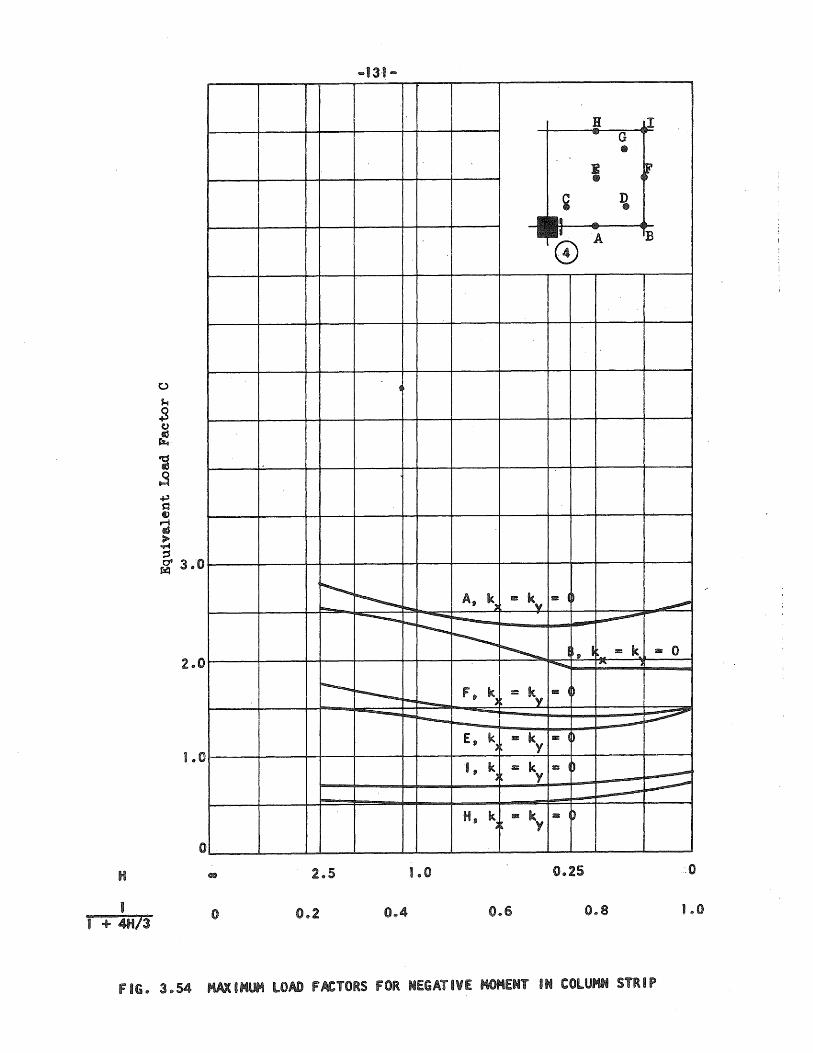
... 13·1 ...
H LI - G •
:I .f II
¥ D • --- IB
0 A
t
~ ~ A. k, III: k III:~
'"'- """'" ·v ~ ----... r- ............. F--- ------...............
~ ~ I • I == Ie. = 0
.......... ''''' 2 .. 0
r---.. t---- ~. &rl == &r - l~ r--"'""--. ., n, .... y
~ r--~ ~ -1.,0
E. k~ = k. == I~ . Y
I • k == k = ID ---~ y ~
HII k, == k - ~ , y
o 2.5 1.0 0.25 .0
+ 4H/3 o 0 .. 2 0 .. 4 0 .. 6 0 .. 8 1 .. 0
FIG. 3.54 MAXIMUM lOAD fACTORS FOR NEGATIVE MOMENT IN COLUMN STRIP
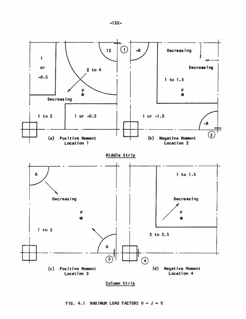
or
-D .. 5
Decreasing
I to 2 1 or ....0.5
Ca> Positive MoMent Location I
Decreasing
1 to 2
p
•
(c) Positive Moment Locat Ion 3
Middle Strip
I
•
II II
Column Strip
Decreasing 1 ------r
I to 1 .. 5
P
•
Decreasing
I or ... 1 .. 5
-
(b) Negative Moment Location 2
- -
1 to 1.5
Decreasing
/: 2 to 2.5
-
(d) Negative Moment Location 4
I
I
fiG. 4.1 MAXIMUM LOAD fACTORS H - J lD 0
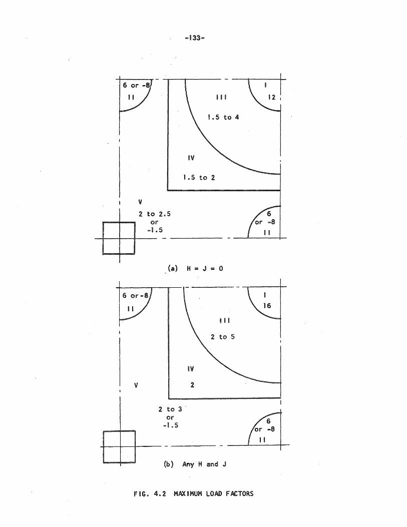
v 2
.... 133 ....
I I I
1 ,,5 to 4
IV
1 .. 5 to 2
to 2.5 0 r
5 ... 1 "
(a) H == J == 0
2 to 3 . or
... 1.5
(b) Any Hand J
FIG., 4 .. 2 MAXIMUM LOAD FACTORS
I
12 I
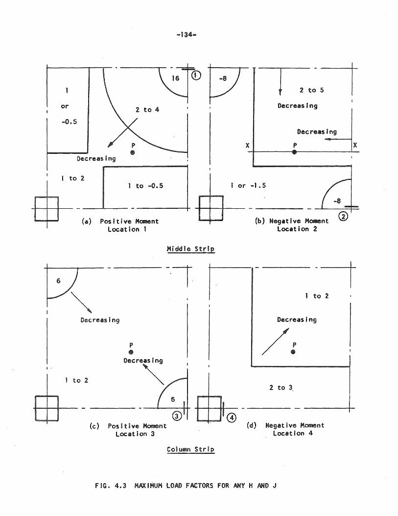
I,
-- - !
or 2. to 4
... 0.5
Decreasing
to 2 1 to -0 .. 5
(a) Positive Moment Location 1
... 134-
Middle Str1e
-·1
1 t
Decreasing
o 2
P
• Decre~
(c) Positive Moment Locillt ion 3
Column Strip
Decreasing
Decreasing
x P
1 or .... 1.5
(b) Negative MOMent Location 2
x
-I
I
I@
1 to 2
Decreasing
/: 2 to 3,
(d) Negative Moment location 4
I
FIG. 4.3 MAXIMUM LOAD FACTORS FOR ANY H AND J
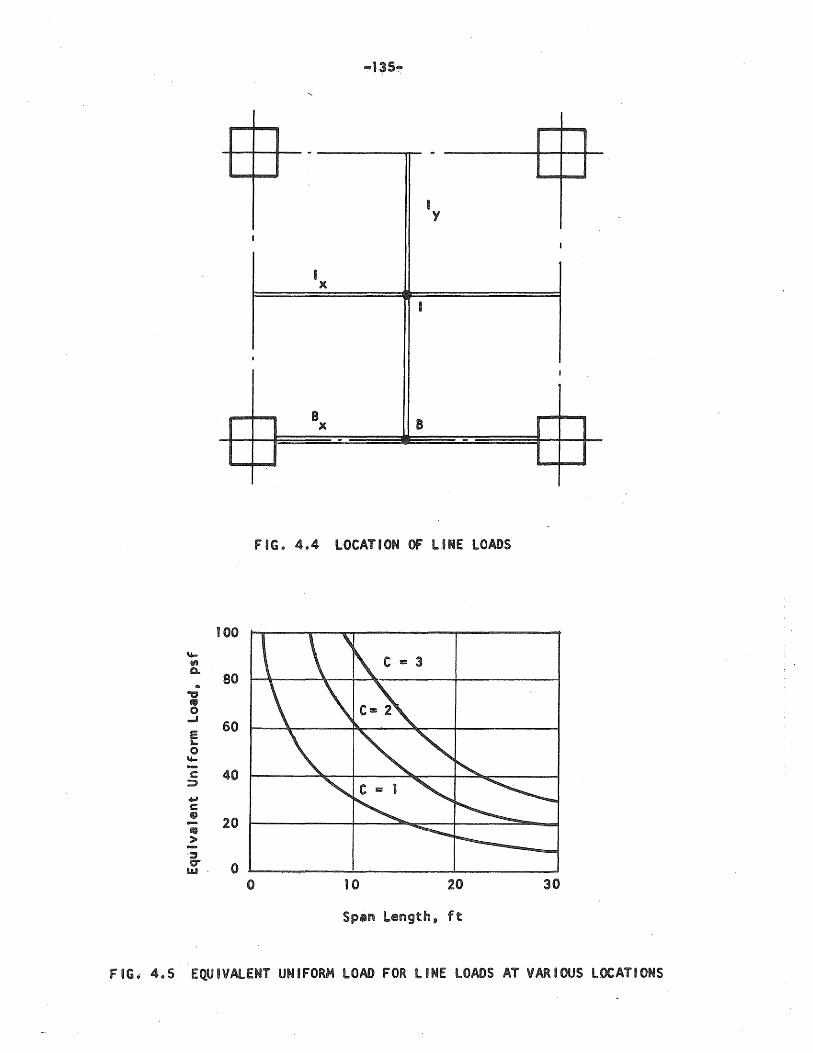
.... 135 ....
- -
I Y
I I
I x
I
I
I
B x B
- -
FIG .. 4 .. 4 l'OCAT ION Of L.' ME LOADS
100
"'-en Q.
80 .. ."
" 0 ...J
60 E .... 0
"'-c 40 ;:) .. c GI)
20 " > '::;, 0" 0 L!IJ .
0 10 20 30
Span Len9th~ ft
FIG .. 4 .. 5 EQUIVAlENT UNIFORM LOAD FOR LINE LOADS AT VARIOUS LOCATIONS

-136-
APPENDIX A: TABULATION OF INFLUENCE COEFF~CIENTS
In this appendix are tabulated the influence coefficients for o
the four moment locations designated 19 2p 3 D and 4 in Figo 2010 These
moment locations are shown on the figures in this appendix by a heavy
short lineo The moment at these locations acts perpendicular to the
section indicatedo
The unit moment p mp at one of the moment locations produced by
a concentrated 10ad p Wp at any node point P is
m = Influence Coefficient at Point P x W x Scale Factor
A negative influence coefficient indicates a reversal in sign of the unit
moment from that normally.occurring at the location with all panels loaded.
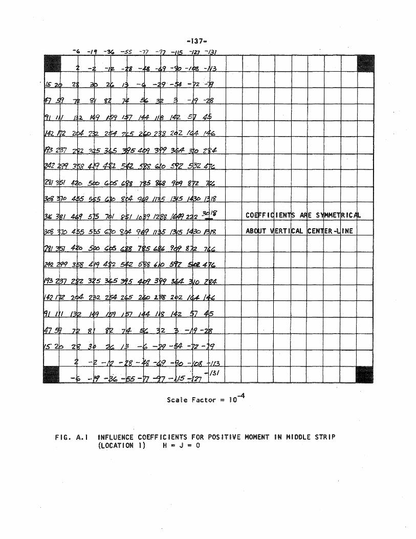
AS
Scale Factor = 10-4
FIG. A.I INFLUENCE COEFFICIENTS FOR POSITIVE MOMENT IN MIDDLE STRIP (LOCATION 1) H = J = 0
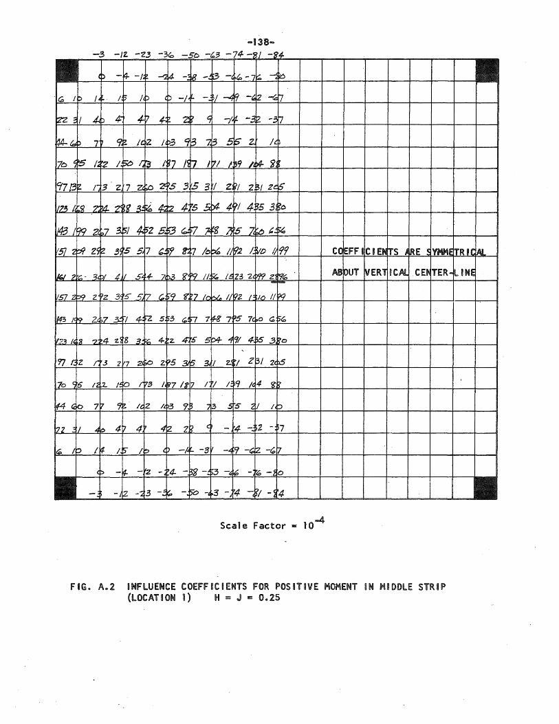
·-138 .... -3 -/l. -Z3 -3b -
Scale Factor = 10-4
FIG. A.2 INFLUENCE COEFFICIENTS FOR POSITIVE MOMENT IN MIDDLE STRIP (LOCATION 1) H = J = 0.25
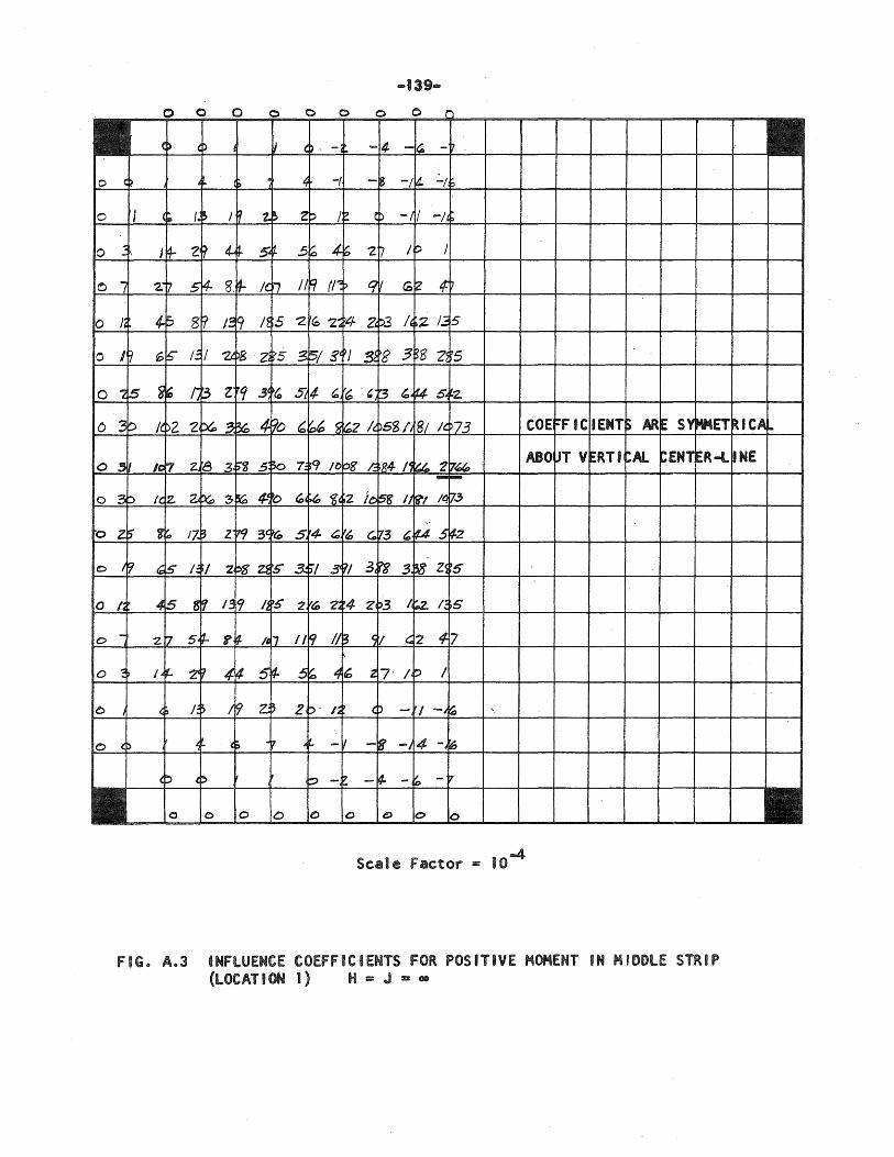
.... 139-
0 0 0 ~ c 0 0 0 i
() (P ~ ~ (~. - -14 - I~ -~
o C~ A"- i:i . ~ -f, -~ -j ~ ~(,
0 J (~ I~~ / 0/ z.~ Z, I:~ eD -/ I -h~
!O ~I. J~ 21 ~ 4..~ ~~ .5 ~ 46 27 I' J
o i 2"17 5 ~ 8 ~ /(. ~7 /I~ (r) qll Gtz " 10 /; 4-~ 8 ~ /'3. '9 /~ ts "2 ~~ 'Z~ ~£f Z p3 ;, :2. Ij 15
10 11 G~ IE. II 'Z~ ~8 2: ~5 3 ~/ 3( il ~ >8 3 ~S Z: ~5
o "2 15 ~ , Ii ~ z rq .3~ ~, 51 14 , r~ ., t3 ,. 145-~z
o 3 ~
o .511
10 3:>
·0 Z5'
o I~
a 14
o -
o :~
6
o (~
Ie )2 '21 ~.3 ~4 ?o ~ ~6 ~ ~2 It. P5gl1 'SI /(. )73
/0 F7 z, r8 3· r;g 5: ~ 7: ~9 If) 08 ~ ~84- " ~2 7"' ...... -It. iZ 21 :lG:>~ !5tD 4-~ b , ;~ cg, ;2 it) ~g II "', Iq 7.3
"
g ~ 17, ~ Z 79 3( ~{D 5 '4- G;, ~ Go 73 , fA.-S rl-2
c:; l5" I~~I 2 ~8' ~ r.5"S ~/ 3 ~/ 3, f8 3-M' z~ rs 4 ~ 8~ 15:9 /J rs 2 r~ 24 ~4 21 p3 I I;.z /~ ~5
Zr? 5~ f'(/. /&17 1If:/ II~ ~tJ '2 417 i'
14- '2''(/ 4 ~ 5~ 6~ 41r:;; 2- 7'/D /
G, I ~ I ~ z:~ 2 :>. I;'~ <:::> - '/ -J~ ,
~:. c:; -'7 ,ill.. - J - g -I 4 -:6
(' (' ::> -~ - 4- - ~ - 7
0 0 0 D 10 0 t!J 10 10
-4 Scale Factor = 10
COE rF IC IIENT $ M ~ S·' , ... ,,-~ T mt.1
ABO' ~T V ER' " ~Al ~f."l ~R-l
FIG. A.3 INFLUENCE COEFFICIENTS FOR POSITIVE MOMENT IN "fDDLE STRIP (LOCATION 1) H = J = ~
1'(1 CAl.
INE
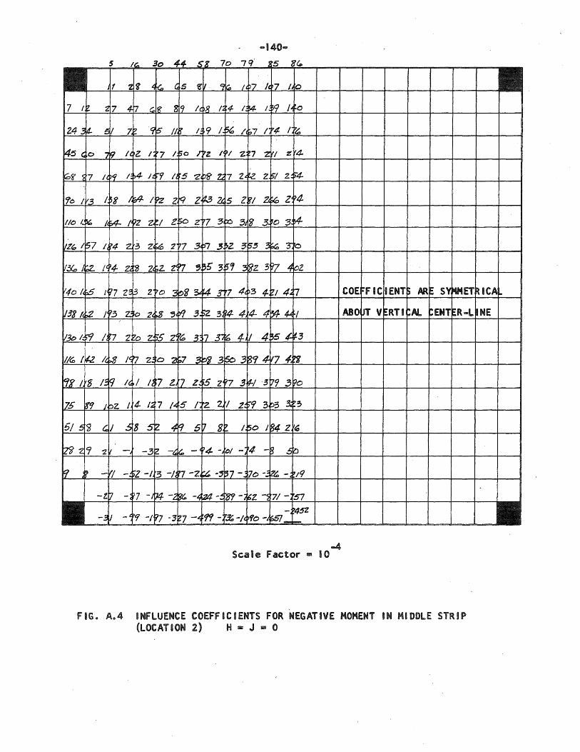
-140-
~ Scale Factor m 10
FIG. A.4 INFLUENCE COEFFICIENTS FOR NEGATIVE MOMENT IN MIDDLE STRIP (LOCATION 2) H = J - 0
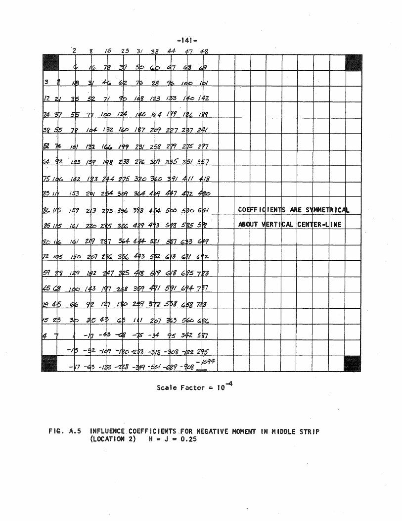
~ Scale Factor = 10
FIG. A.S INFLUENCECOEFFICIENTS.FOR NEGATIVE MOMENT IN MIDDLE STRIP (LOCATION 2) H = J E 0.25 .
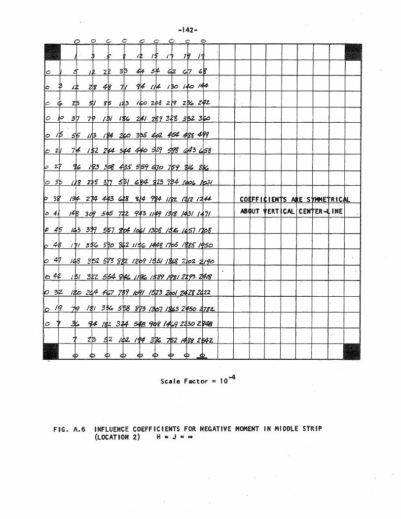
-142-
~ Scale Factor = 10
FIG. A.6 INFLUENCE COEFFICIENTS FOR NEGATIVE MOMENT IN MIDDLE STRIP (LOCATION 2) H ~ J = •
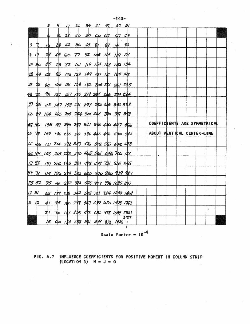
~ Scale factor = 10
fiG. A.1 INfLUENCE COEFfiCIENTS fOR POSITIVE MOMENT IN COLUMN STRIP (LOCATION 3) H z J = 0
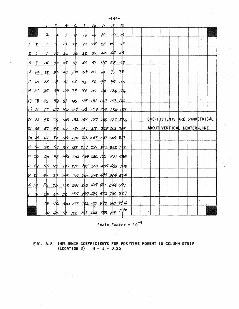
-144-
Scale Factor ==
fiG. A.a INFLUENCE COEFFICIENTS FOR POSITIVE MOMENT IN COLUMN STRIP (LOCATION 3) H = J = 0.25
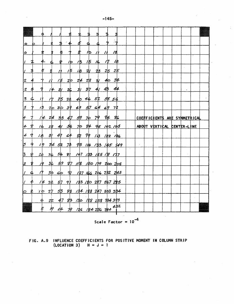
0 ~
0
J ~ ..
/ !
2 ,,~
. Z ~;
3 GFo
;5 -.,
t -I ~ cz:)
-/- c:
~ (~
~ P
lZ -~~
I GF»
/ .c~
[0 ;
-145 ....
c~ J J ~. ~'" . -:~ ! 1:. ~
J ~ ':~ .. ~I- £" G~ ~~ .. ~ ~:j
~~ , ~~ ... ir ~ I~ /,~ h 11-
4!~ (t> ~~ /b I:!> 15 1<1m /7 h~
~~ ~ /' /5 /c8 '2 ~ 2 d 2 5 2; ~
"" I I.) 20 z4 z 18 E I -4 o 3 ~
~ I tp.. 2.1 2(~ :J'J 3 ~ 4- I 4.:. ~ 4-~
J /7 2. 5 3 ... 4-o 4. ~ S ~ .~ '5' 5(~
I ~ 'Zo 3 ::> 3~ t/- ~ .6 '7 ~. tf. ~ 9 7~
Itf.o z 4 ~ 5 4-7 5 9 74 ::> 74 '1 <l ~ f,~ COEI
/(~ z~ 4 I ~;; 7,:; S ~ 9 5" /~ :>2. /t. )5 ASOt
I e.~ ~I I 4-'1 ~~ 9- ~ 9 '1 h 3 /4 rz r. ~
J~ ~ ~ 5~ 7.~ 9 ~ II ~ /~ ~3 /' ;ts~ '49
~~ 3c ~ S ~ S> It. 7 /. ~ /, 5"5 / ~I I"; '7
I~ 3~ ~ ~ i9 ~ 17 1/ 8 I~ ;0 / r9 2 ~~ bg
!' ~ .3, ~ ~ p ~y I tz7 ~ ~ '24 ~ Z. 5Z 2 ~
I~ 3, ~ 5 17 l:f I I:' ~3 /~ ~o 2: ~7 Z ~7 2J ~6
-, :> 2 7 5: ~ ~fJ 1:-,~ /' ~8 2, "7 31 '3 3. >4-
(:> Z ;Z ~ ~7 <j/ I~ I:' ro I~ ~8 2 5g 3 343( "3
S 19 4-~ 7 ~ /~ t' I ~4Z 5(;;3- f..+4-- ~z.
-4 Scale Factor - .0
~f IC I Elm >AR E ~T ¥'Itt
JT V ERT. :Al botrlll t.K-L
FIG. A.9 INFLUENCE COEFFICIENTS FOR POSITIVE MOMENT IN COlUMN STRIP (LOCATION 3) H B J B 1
~ ICAI ..
INE
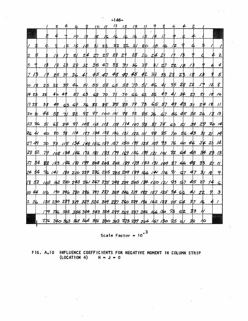
124-
-146 .... 12 /2. /2 II 9 8 ~ 4- z
_3 Scale Factor • 10
FIG. A.l0 INFLUENCE COEfFICIENTS FOR NEGATIVE MOMENT IN COLUMN STRIP (bOCAT80N 4) H 8: J - 0
z.
s
/0
II
I
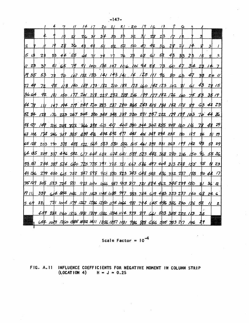
II 14-
-147'!"'
~I • 20 /9 /
-4 Scale Factor e 10
FIG. A.ll INflUENCE COEffiCIENTS fOR NEGATIVE MOMENT IN COlUMN STRIP (lOCATION 4) H = J = 0.25
17
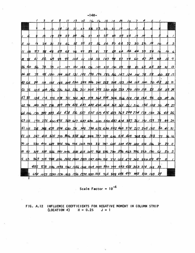
~ Scale Factor = 10
FIG. A.12 INFLUENCE COEFFICIENTS FOR NEGATIVE MOHENT IN COLUMN STRIP (LOCATION 4) H = 0.25 J - 1
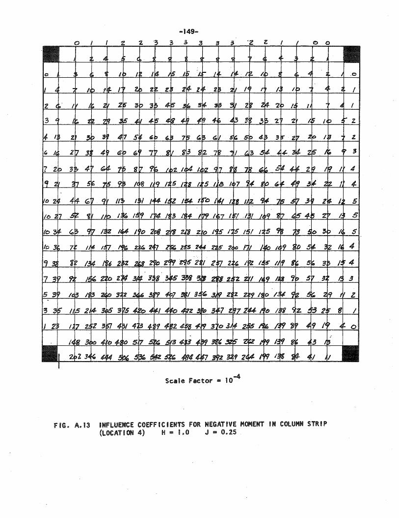
-149 ....
-4 Scale Factor - 10
FIG .. A .. 13 INFLUENCE COEFFICIENTS FOR NEGATIVE MOMENT IN COLUMN STRIP (LOCATION 4) H - 1 .. 0 J • 0 .. 25
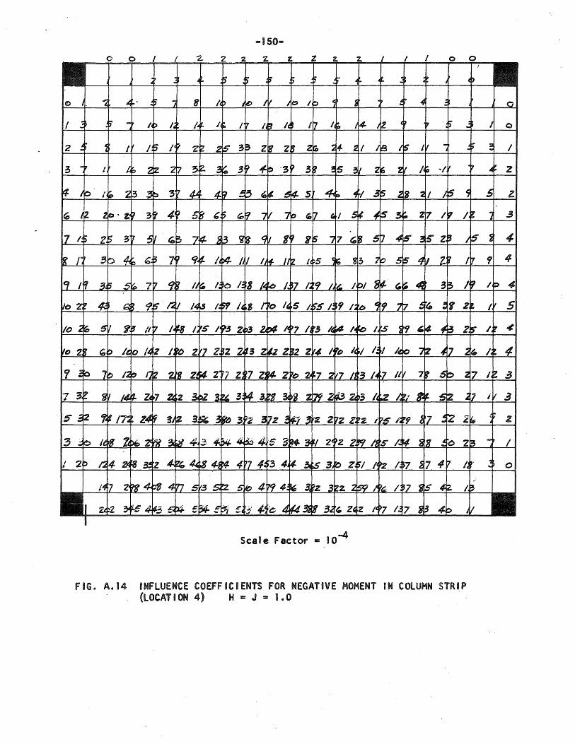
Scale Factor - 10-4
FIG .. A .. 14 INFLUENCE COEFFICIENTS FOR NEGATiVE MOMENT IN COLUMN STRI.P (LOCATION 4) H - J = 1.0
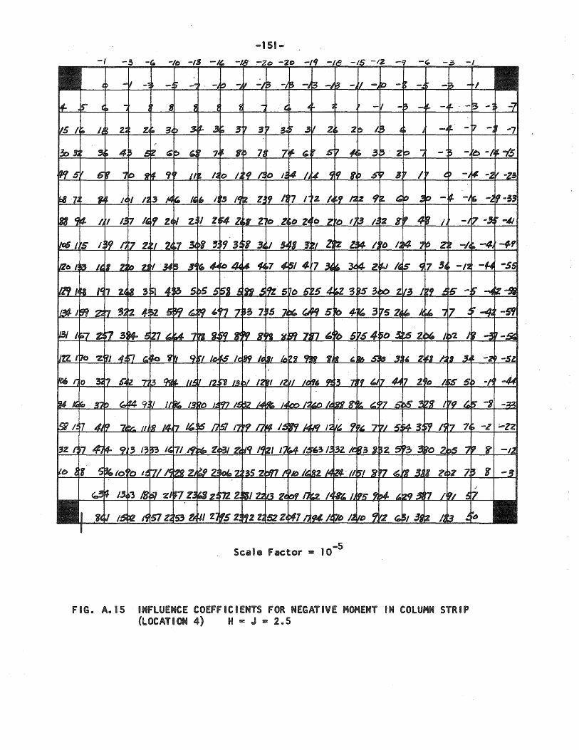
-151-
-5 Scale factor - 10
FIG. A.IS INFLUENCE COEFFICIENTS FOR NEGATIVE MOMENT IN COLUMN STRIP (lOCATION 4) H = J - 2.5


![THIN CYLINDRICAL SHELLS SUBJECTED TO ......equation will now be applied to an infinitely long thin cylinder loaded, as shown in 1946] CYLINDRICAL SHELLS SUBJECTED TO CONCENTRATED LOADS](https://img.pdfslide.us/doc/110x75/5e976cdbab147d7e621358aa/thin-cylindrical-shells-subjected-to-equation-will-now-be-applied-to-an.jpg)
![CONCRETE FLOOR SLABS ON GRADE …civil.colorado.edu/~silverst/cven4830/design_of_Slabs[1].pdfCONCRETE FLOOR SLABS ON GRADE SUBJECTED TO HEAVY LOADS ... BASIS OF FLOOR SLAB ON GRADE](https://img.pdfslide.us/doc/110x75/5aae3b7a7f8b9a07498bd530/concrete-floor-slabs-on-grade-civil-silverstcven4830designofslabs1pdfconcrete.jpg)
![CONCRETE FLOOR SLABS ON GRADE SUBJECTED TO HEAVY LOADSceae.colorado.edu/~silverst/cven4830/design_of_Slabs[1].pdf · concrete floor slabs on grade subjected to heavy loads ... concrete](https://img.pdfslide.us/doc/110x75/5a796a617f8b9a770a8b9064/concrete-floor-slabs-on-grade-subjected-to-heavy-silverstcven4830designofslabs1pdfconcrete.jpg)


![CONCRETE FLOOR SLABS ON GRADE SUBJECTED TO HEAVY …civil.colorado.edu/~silverst/cven4830/design_of_Slabs[1].pdfconcrete floor slabs on grade subjected to heavy loads depart ments](https://img.pdfslide.us/doc/110x75/5f2fc07209e2f603340c5c0d/concrete-floor-slabs-on-grade-subjected-to-heavy-civil-silverstcven4830designofslabs1pdf.jpg)