RESEARCH BULLETIN 949

AN ANALYSIS OF THE PRICES OF HOGS, WHOLESALE AND RETAIL PORK PRODUCTS IN

OCTOBER 1963

CENTRAL AND SOUTHWESTERN OHIO

G. F. HENNING

J. H. LEWIS

OHIO AGRICULTURAL EXPERIMENT STATION - - WOOSTER, OHIO

SECTION l Introduction

CONTENTS

* * * * *

The Sample -~ ~~-- ~~ -~-~~-~~-~-~-~ ~~~-~~~~~ ~~ -~-~~~ ~~-~-- -~~~ ~~-~

Basic A;wmptions and Limitatiom oL Data

SECTION 2 The l\Iovement o1 Ohio Hogs lor Slaughter

,, ~~~ ~ J

5

i

from the Fir;t 1vlarket ~- ~ ~~~~ ~~~ -~ ~~ -~~ ~- ~--- ---~ _ ~-~ -~ _ ~~~~-~~~~~-~~~~ i

SECTION 3 Size of l\Iarket Area;, Trttcking and Marketing

Charges Paid by Fanners ~- ~~~-~-~-~~- ___ _ ~--~-~-~-- ~ ~-~~~~~-~~~~ 9

SECTION "1 Price; Paicl to Farmen for Slaughter Hogs

Sold in 0 hio ~~~~~- ~~~- ~~-~ -~ -~~ ~~~~-~~~~~~~~~ ~~~ -~ ~-~~-- ~~-- ~~-- -~-~~~~ - 13 4a Net Price~ Compared by l\larket A1eas in Ohio ~~~~-~~~~-~~~~ 14

4b Net Price; Compared by Types oi Markets _ ~-~ ~~ -~~~-~~~-16

~Jc Net Price; Compared by Si;e oJ l\larkets (Volume) ~~~~~~~~18

SECTION 5 Prices in Sampled Area Compared to Selected Markets ~~ ~~~-- ~ ~18

SECTION 6 Transportation Rates (Co~t;,) Compared to the Price;

Paid for Slaughter Hogs by l\Iarket Areas -~-~- ~ ~ ~~~ _ ~~~~~~~~~~~~~- 21

SECTION 7 The Procedure in the btablishment ()f the Dailv

Market Price lor Hog~ _ ~~~--~~ -~ --~~~~-~~~~~~~ ' ~ ~ _ ~~~~~~~~~~~~~- 23

SECTION 8 Prices tor Selected Wholesale and

Retail Pork Products in Ohio

SECTION 9

--25

Summary and Conclu;,iom ~~ -~~~~-~-~--~~~~-~~~-~~~-~~--~ -~~~- ~ ~~~~~-~ -~ ~- ~~ ~~~-~-3~1

APPEND IX ~~~~-~~~~ ---~~~ -~~~~~~~~~----- ~~~~~- ~~~~. ~~ ~~~~~~~--~~ -~~- ~~~~~~~- _ -~ -~- ~-~~-~~--~ _ ~~~-- 3 5

AGDEX 848 440 1 0-63-3M

An Analysis of the Prices of Hogs, Wholesale and Retail Pork Products in Central and Southwestern Ohio

G. F. HENNING J. H. LEWIS

Sedion 1

INTRODUCTION The production and marketing of hogs and the ~laughtering. proc­

essing, wholesaling, and retailing of pork and pork products to con­sumers are important Ohio industries. Annual sale of meat animals (cattle, calves, hogs, ~heep and lambs) has provided from almost $280

million to $330 million cash farm income in Ohio during 1958, 1959 and 1960.1 This wa~ approximately 28 percent to one-third of Ohio\ total farm receipts from sales of agricultural commodities.2 Of the amount received from the sale of live5tnck, 40 to 52 percent came from the sale of hogs.3

Because livestock holds the important position that it does in Ohio agriculture, the availability of adequate markets is vitally important to farmers when marketing livestock. "\Vide variations in the livestock enterprises in various sections of the &tate and in classes of livestock on individual farms make the job of marketing livestock a complex one. Continuing changes taking place in the technolo~y of production and processing of livestock also complicate the marketinp; problem. The impacts of change at one level have repercussions and implications for other levels of production, processing, and distribution.

The efficiency with which Ohio hogs move through the various marketing steps in this area into the hands of the consumer, relative to hog prices in other producing areas and at major slaughter point~. af­fects the profitability of ho~J; production in Ohio. On the other hand, the seasonal year-to-year and cyclical pattern of hog production affects per unit processing costs of meat packing firms and thereby affects local hog prices.

As of March 1, 1960, according to the United States Department of Agriculture, there were 238 meat r.laughtering establishments in Ohio.4

Of these, 32 were under federal inspection and 206 were under state or city inspection." On December I, 1960, according to the Ohio office of the Packer Stockyards Administration and the Ohio Department of Agri­culture, there were 63 auctions. 128 local livestock markets or concentra· tion yards, three terminal markets (Cincinnati. Cleveland :md Dayton) , ?7 pac~er buying stations and 344 registered livestock dealers operating m Oh10.6

11958 Ohio Farm Iru:ome. Bulletin No. A.B. 306, Ohio f\tate Univcrsitv. •Ibid. 'Ibid. •Number of Livestock Slaughter Plants March I, 1960: lJnited States Department of Agriculture Ag• riculture Marketin~ Service Crop Reporting Board, Washington. D. C .. August 1960. '

'Ibid. "Ohio Department of Agriculture, Division of Animal Industry, Columbus, Ohio (unpuhlishe<;l listing), and Packer St<><:kyards Administration.

3

Table l - Cash Receipts from Livestock Marketing in Ohio, 13 North Central States and United States, 1959

State

Ohio

'I otal 13 North Central States

Total U. S.

Percent 13 States

Cattle

Thousands $ 145,401

~4.430,595

:<17.R93,095

Ca:-.h Receipts from Livestock Markcttngs Hogs Sheep and Lambs

Thousands j;: 128,433

S2,331,322

~2.806,084

Thousands

::;, 10,667

:1:> 156.:l71

$ 336,491

Total

Thousand; ;-, 284.501

:- li.918 2H8

~11,03!\,(i70

are U. S. 56.13°70 83.08 Of, 46.47% 62.69~1,:

Source: Meat Animals, Farm Production, Disposition and Income by States, 1959. United States Department of Agriculture.

The North Central States, of which Ohio is a part, encompasses the area of greatest hog concentration in the United States. The&e 12 states plus Kentucky account for about 80 percent of the total United States hog production (Table 1). In this region, major shifts are taking place in the relative importance of competing market institutions. Currently in Ohio, there is much uncertainty concerning the efficiency with which pork and pork products move through market channels to the consumer and the possibilities of developing methods of improving the system. There were observed instances in which locally produced livestock wa' moved out of an area to slaughtering plants and at the same time pack­ers within that area were obtaining part of their slaughter hogs from outside producing areas at fairly great distances from the plant. Also, pork and pork product~ frequently were moved out of the locality of slaughter and processing in Ohio at the same time large quantities of pork products were being shipped in from meat packing plants, princi­pally from mid-western points. For example, in 1958, large quantities of pork and pork products were ~hipped into the southwestern Ohio area by distant packers in the mid-·west, although hog slaughter {rom local packers provided pork and pork products in excess of local con­sumption requirements. These and similar observed livestock and meat movements suggest that livestock and meat movements in the area may be excessive in that live-to-wholesale-to-retail costs and margins may be larger than would be necessary under a more efficiently organized mar­keting system.

The cost of marketing me:tt takes more than 40 cents of each dollar spent for meat at retaiJ.7 Reductions or increases in livestock and meat marketing costs could have a significant influence on the retail cost of meat to consumers and on returns to farmers for livestock. This indica­tion of inefficient movements may arise from several causes. First, ot course, these movements may be grossly overestimated and simply repre­sent short-run corrective action of the market. Second, these movements may reflect a need to adjust to market conditions, such as geographic differences and seasonality of marketings and grade composition of mar-7Podc Marketing Margins and Costs, United States Department of Agriculture, Agricultural Marketing Service, Washington, D. C.

4

ketings, geographic differences in livestock quality and geographic dit­ferences in consumer tastes and preferences_ A third possibility is that these movements may represent real and continuous inefficiencies arising from the market imperfections due to limited competition in some areas, inadequacy of market information available to firms participating in the market, lack of response of the firms to market incentives or other market causes.

The growth ol food-handling chain store organizations and ~uper­markets in the past decade has betn a major factor in bringing changes m handling· of meat and meat product<.. Forward retail price-setting influences the prices of slaughter livestock a week or two later. The concentration of retail huying in a relatively few hands may be a power­lui influence on prices of slaughter livestock, especially in the short­run. It is estimated that about 75 percent ol the food is now handled by chain-store and supermarket organi1ations.

This concentratirm of buying power by retailers has accelerated the trend towards decentralization of the parking plants and the closing ot branch houses through which meat was formerly distributed. The ef­fects these change~ at the wholesale level are having on the price ol slaughter livestock need to be examined in terms of their probable effect upon margim and price variability to producers, middlemen, and con­sumers. A large chain-store organization covers a wide territory and follows essentially the same purchasing and merchandising program wherever it operates. Thus, the rigidity in pricing policy may be ex­pected to reduce normal spatial price differentials.

The general objectives of this study were first to analyze the market price structure and pricing accuracy for slaughter hogs for the major hog-producing areas in Ohio. These areas which are outlined in Chart I included Columbus and surrounding counties, Cincinnati-Dayton and surrounding counties, six South Central counties, and eight West Central counties_ The second objective was to analyze the marketings structure in the wholesaling and retailing of pork and pork products within these same areas. The Sample

Conditions of hog· production, marketing and slaughtering vary within the state_ Areas were delineat<.>d to provide sample areas where conditions were comparatively homogeneous with respect to hog pro­duction and marketing practices. Within these areas, price and receipt data were assembled oYer specified time periods relative to the dominant pricing influence operating within the area as this influence is related to terminals, auctions. local markets (concentration yards) , parkers and packer buying stations.

This ~tudy was a part of a regional research project conducted by the participating states represented by the North Central Livestock Mar­keting Research Committee. Each participating state was responsible for drawing its own initial sample. However, the technique used by all states in drawing the actual samples of liYestock markets was designated specifically by the Regional Coordinator.

5

CHART I

Location of the General Sampled Are<~ in

which Data were Obtained from Five Distinct Hog Marketing Areas, 1959-60,

A total of 46 markets were sampled in Ohio's major hog producing area. These were categorized under three major classifications, namelv, by areas, by type of market and by size of market. '

The general area of study shown in Chart I was broken down into five distinct marketing areas and will be designated throughout thi~ study as areas A, B, C, D, and E, respectively. These area~ were clas­sified primarily on the basis of the marketing· system. Area A is charac­terized by local markets as the dominant marketing organization. Area B is ch<!racterized by packer buying station marketing plm a very small terminal market. In Area C the terminal market is the dominant mar­keting organit.ation. Area D includes a combination auction local mar­ket type of organization. Area E represents a cross-section oi all types of marketing structure, with the exception of the terminal system.

Of the 46 markets sampled, 10 were located in Area A; 4 in Area B; 1 in Area C; 15 in Area D and 16 in Area E. The sample when broken down by type of market included 16 local markets (concentration yards), 15 combination auctions and local markets, 13 packer buying stations and two terminal markets.

The markets were then classified according to volume of hogs han­dled on a weekly basis. Markets which handled 750 or less per week were designated as small volume markets; markets handling 751 to 1250 head of hogs per week were classified as medium volume markets and markets handling 1,251 head of hogs and more per week were classified as large volume markets. Of the 46 markets sampled, 21 were small volume markets, 15 were medium volume markets and 10 were classified as large volume markets.

Data were obtained from September 14, 1959, through October 9. November 16 through December 1 I, and February 15. 1960, through February 26, making a total of ten weeks. For these periods a total vol· ume of 449,506 hogs weighing from 180 to 260 pounds were marketed. Of this amount, 56.8 percent were ~hipped to buyers or packers located in Ohio and the balance to 10 other states.

6

Basic Assumptions and Limitations of Data In analyzing the data, it was necessary to make some basic assump­

tions in developing methods of analysis. These asmmptions were: (1) The prices quoted for variom weight brackets of slaughter hogs were the actual prices paid; (2) Market price quotations were based on grad­ing that was substantially uniform from day to day throughout the pe­riod for all market>; and (3) \!\There prices were reported as a range, the level of market price was represented by the midpoint of the range. Of course, the assumptions at times may have definite limitations such as: (1) The mid-point of the quoted price range may vary from the average price paid in a given period. (Account of the number of animals that are sold at different prices within the price range was not considered, thus making it difficult to determine the actual weighted average price paid. Thus, the wider the price range, the Jess significant is the mid­point likely to be as a price mea>ure.) : (2) The grading of hogs may vary from day to day at a given market, and may vary between markets on a particular clay; (3) The wider the weight range included in a single price quotation, the less significant is the mid-point likely to be as a price measure; and (4) The sample under analysis does not take ac­count of variations in quality within a weight division. Because of these limitations, the term "average" is used.

Section 2 THE MOVEMENT OF OHIO HOGS FOR SLAUGHTER

FROM THE FIRST MARKET

Table 2 shows the destination by states of hogs marketed through the sampled markets. In this section an examination in more detail will be made of the movement within Ohio and to other states. West­ern Ohio, along with lndiana, parts of Northern Kentucky, and South· ern Michigan is considered as the eastern part of the Corn Belt. The movement to points outside Ohio from this area is primarily to the eastern states. However, based on estimates made by William H. Lim­mer,' Ohio consumed more pork than was marketed by Ohio producers for the year 1958. Limmer estimated that the marketings were only 91 percent of consumption. The percentage for beef was 49 percent, veal '14 percent, and lamb and mutton 79 percent. \1\T"ith Ohio consuming more pork than is produced in the state, then outside processors will seek a market here for pork, while Ohio processors may be inclined to buy live hogs from Indiana and other states to the west in order to sell more pork to retailers in Ohio. There also is a rather large movement into Ohio of carcass :md processed meat from processors in other states principally from the west.

From the sampled area of ..J-6 markets, 43.2 percent of the slaughter hogs were marketed and transported to processors in ten other states. Pennsylvania and New Jersey received 28.~ percent. Packers located in these two states were the important out-of-state buyers. Virginia and West Virginia buyers received another 10 percent and the balance of ~

'William H. Limmer, Market Livestock Available and Analysis of Livestock Market Location in Ohio, Masters Thesis, Ohio State Univer;ity, 1959.

7

Table 2- Nwnbet· and Percent of Slaughtet· Hogs Shipped to Various Areas Within Ohio and to States Outside Ohio from the Sampled Area During Teii Weeks of 1959 and 1960

Area and State Number of Head Percent Ohio

Southwestern Area 74,265 16.5 ·western Area 64,971 14.5 Central Area 49,926 II. I Northeastern Area '12,35g 9...1 Southea~tern Area 20,622 4.6 Northern Area 3,237 0.7

Total Ohio 255,374 ~ Pennsylvania 83,069 18.5 New Jersey 44,047 9.8 Virginia 23,622 5.3 West Virginia 21,026 4.6 New York 9,237 2.1 North Carolina 4,559 1.0 Michigan 3,966 0.9 Kentucky 2,436 0.5 Indiana 1,539 0.3 Connecticut 731 0.2 Total 449,506 JO(iJ)

percent went to New York, North Carolna, Connecticut, Kentucky, Michig·an and Indiana. If the sample had included another 30 or more Ohio counties, no doubt hogs would have been sent to Mas&achusetts, l\Iaryland, and other eastern states, which are heavy consumption areas.

There is one important factor that may have influenced large pur­chases by processors in Pennsylvania. Armour and Company suspended operatiom at Columbus on July 11, 1959. The plant had been receiv­ing a large portion of hogs from three Armour buying stations. operat­ing within the sampled area. These buying stations remained in op­eration after the closing of the Columbus plant and diverted their pur­chases primarily to Am10ur plants in Pennsylvania.

Considering the movement of hogs within Ohio, the 46 markets in the sampled area sold 56.8 percent of their volume during the ten week period studied to slaughterers located in Ohio (Table 2) . Buyers from the southwestern, western and central Ohio areas took the largest por­tion, 42 percent. Very few hogs were sold to slaughterers from the north­ern part of the state. It was interesting to note that slaughterers in the northeastern part of Ohio purchased an impressive volume of the sampled area hogs although they may have been closer to other sources. The question may be raised as to whether quality and price were fac­tors which influenced their decisions. It would have been interesting to have studied the distribution of slaughter hogs from the 30 or more counties to the north of the 5ampled area2 and to have compared the pattern of distribution from that area with the sample in this study. 2Funds were not available for a study of this si~e.

8

With this background the pattern o( movement of slaughter hogs from, within and to Ohio is established. In view of the fact that Ohio consumes more pork than is produced, and that Ohio is located on the eastern edge of the Corn Belt, there is active competition for Ohio hogs. Eastern slaughterers are competing actively with Ohio slaughterers for Ohio hogs because of relative lowc:r procurement costs, unless the price is forced too high. On the other hand, mid-western packen keep the Ohio packen. in line by competing aggressively for sales of pork pro­ducts to Ohio retailen. However, eastern and Ohio packers can switch their live hog purchases to the Central Corn Belt if procurement prices become more favorable. Thus, net costs to each packer at his plant are the determining factors considered in arranging purchases. Of course, such other factors as ~hrink, dressing percentages. quality of hogs bv areas, unifonnity of grading, furnishing· hogs that meet the grade stand­ards of the packer, cordial, friendly and honest day to day business trans­actions are important to slaughterers in purchasing their hog supplies from Ohio market&. It is this keenly competitive operation that is be­hind the purchasing of hogs at Ohio markets and the daily pricing by the numerous markets included in this study, as well as other markets located in the Eastern Corn Belt.

Section 3 SIZE OF MARKET AREAS, TRUCKING AND MARKETING CHARGES PAID BY FARMERS

With numerous small markets opere~ting- in Ohio, market areas are not distinct but overlap with each other. Table 3 shows the distances involved in marketing hogs. Each market manager in the sampled area was asked to give the market area where he obtained 50 percent and 75 percent of his volume for the past year. Almost 85 percent of the mar­kets obtained 50 percent of their volume within 15 miles and 40 percent within 10 miles. Only 30 percent of the markets received 75 percent of their marketings beyond 20 miles.

Most all hogs were transported to market by commercial truckers or by farmers who had their own truck-;. A small volume was brought in by trailers pulled by passenger cars. Most trucking was done with two axle trucks having livestock racks 14 to 18 feet in length. For longer hauls to terminal markets semi-trailer trucks were used. Semi-trailers

Table 3- Size of Market Area From Which 50 Percent and 75 Percent of Volume was Received by the Market~ Studied

Radius

Up to 9 mile& 10 to 14 miles 15 to 19 miles 20 to 24 miles 25 and over Total

50 Percent Volume

9

40 44 10 6

75 Perrent Volume

14 30 27 21 8

100

were also used to some extent when hauling large numbers of animals I 0 or more miles.

Farmers were charged for trucking livestock to the local markets under three basic methods: (1) per loaded mile; (2) per hundred­weight; and (3) per trip. About 50 percent o[ the yards charged farm­ers on the basis of a loaded mile, about equally divided between 40c and SOc per loaded mile. One yard charged 45c. Another group (20 per­cent. of the markets) charged on the basis of cents per hundredweight of livestock hauled. The most common charges were lOc and 15c for distances up to 30 or 40 miles but usually with a minimum charge of .$3 for a small load.

The balance charged on a per trip basis or some modification of the above varied from minimum of $2 to $8. One market had a mini­mum charge of $2 for less than 5 miles but $4 up to I 5 miles. Another market, on the high side, had a charge of $8 for more than 15 miles.

In Tables 4 and 5 the trucking charges for a load ot hogs weighing 4,400 pounds have been applied to each of the 37 markets furnishing information on this question. These tables show the variation in the application of these trucking charges for different distances.

Truckers, at approximately 40 percent of the yards, charged up to $3 for a load of 4,400 pound& trucked no more than .? miles. On the other hand, at a few markets for the same distance, the charge ranged from $8 to $10.

For trucking 10 miles, the bulk of the charges were from $4 up to $8, for 15 miles from $5 to $8, and for 25 miles $10 or more.

In Table 5 all the rates have been calculated on a per hundred­weight basis for a load of 4,400 pounds to illustrate the variation in the trucking charges for these marketing areas in Southwestern Ohio. Again there is a wide variation in charges. This is became truckers charged definite dollar amount for the time and distance involved in traveling to the farm, loading the livestock, driving to the market, and unloading the livestock. Charges varied and were not as uniform a~ might have been expected.

Marketing Charges Three methods of marketing charges were practiced by the 46 mar­

kets. Of this number 17 were operating on a per head charge, 16 on a per hundredweight basi~ and 13 were making no charges at all. With this variation farmers had to estimate what the net price would be for 33 of the 46 or 71 percent of the markets, Table 6.

The farmer should tramfer per head charges to a per hundred­weight basis for different weight of hogs. A 50c per head charge is 25c per hundredweight for 200 pounds, 20c for 250 pound~ etc. These charges must be deducted when comparing prices of another market which offers net prices.

A farmer should consider other factors in addition to net price for certain markets to which he may ~ell his hogs. One of these is the amount charged for hauling from his farm to the market. If one mar­ket is five miles away and another is 50 miles, the transportation should

10

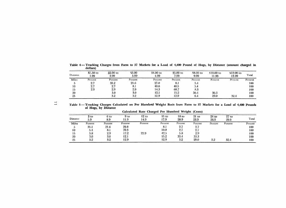
Table 4- Trucking Charges from Farm to 37 Markets for a Load of 4,400 Pound of Hogs, by Distance (amount charged in dollars)

$1.50 to $2.00 to \>3.00 $4.00 to $5.00 to SB.OO to $10.00 to !1:12.00 to Di~tancc 1.99 2.99 3.99 4.99 7.99 9.99 11.99 13.99 Total

Miles Percent Percent Percent Percent Percent Percent Percent Pncent Percent

5 2.7 35.2 21.6 27.0 B.l 5.4 100 10 2.7 2.7 8.1 40.6 40.5 5.4 100 15 2.9 2.9 2.9 14.3 68.7 1!.3 100 20 3.0 3.0 12.1 15.2 36.4 30.3 100 25 3.2 :!.2 12.9 12.9 6.4 29.0 32.4 100

Table 5-Trucking Charges Calculated on Per Hundred Weight Basis from Fann to 37 Markets for a Load of 4,400 Pounds of Hogs, by Distance

Calculated Rate Charged Per Hundred Weight (Cents)

3to 6 to 9to 12 to 15 to 18 to 21 to 24to 27 to Distanc-e 5.9 8.9 11.9 14.9 17.9 20.9 23.9 26.9 29.9 Total

Miles Percent Percent Percent Percent Percent Percent Percent Percent Percent Percent

:) 35.1 21.6 29.8 8.1 2.7 2.7 100 10 5.4 8.1 70.3 10.8 2.7 2.7 100 15 5.8 2.9 17.2 22.9 42.5 5.8 2.9 100 20 3.0 3.0 12.1 15.2 33.4 33.3 100 25 3.2 3.2 12.9 12.9 3.2 29.0 3.2 32.4 100

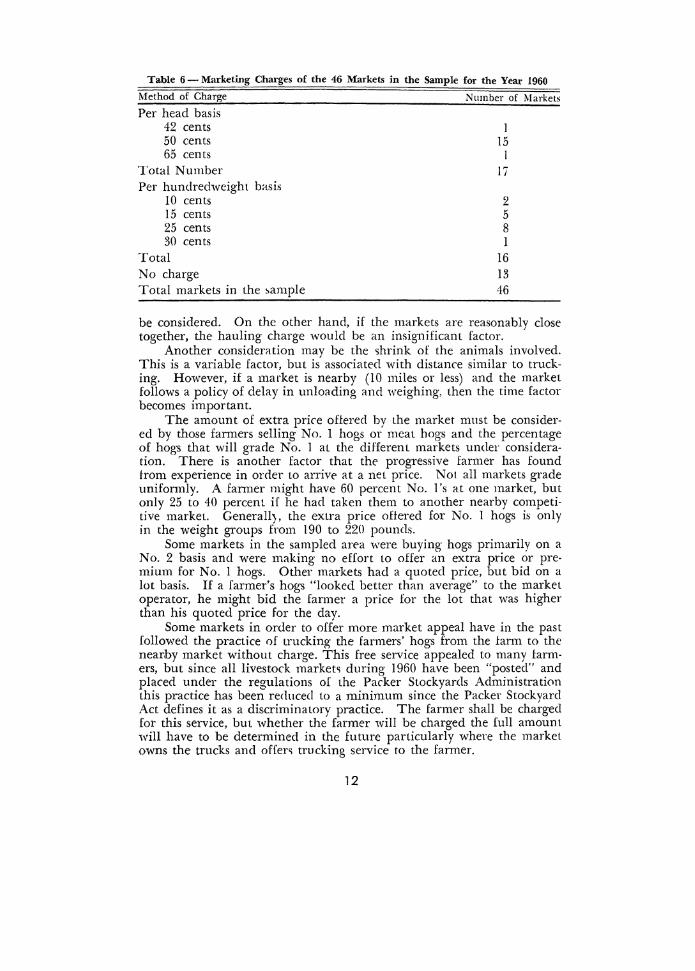
Table 6- Marketing Charges of the 46 Markets in the Sample for the Year 1960

Method of Charge

Per head basis 42 cents 50 cents 65 cents

Total Number Per hundredweight basis

I 0 cents 15 cents 25 cents 30 cents

Total No charge Total markets in the ~ample

Number of Markets

15 I

17

2 5 8 I

16 13 46

be considered. On the other hand, if the markets are reasonably close together, the hauling charge would be an insignificant factor.

Another consideration mav be the >hrink of the animals involved. This is a variable factor, but is' associated with distance similar to truck­ing. However, if a market is nearby (10 miles or less) and the market follows a policy of delay in unloading and weighing, then the time factor becomes important.

The amount of extra price oHerecl by the market must be consider­ed by those farmers selling No. l hogs or meat hogs and the percentage of hogs that will grade No. 1 at the different markets under considera­tion. There is another factor that the progressive farmer has found from experience in order to arrive at a net price. Not all markets grade uniformly. A fam1er might have 60 percent No. 1 's at one market, but only 25 to 40 percent if he had taken them to another nearby competi­tive market. Generall), the extra price offered for No. 1 hogs is only in the weight groups from 190 to 220 pounds.

Some markets in the sampled area were buying hogs primarily on a No. 2 basis and were making no effort to offer an extra price or pre­mium for No. I hogs. Other markets had a quoted price, but bid on a lot basis. If a farmer's hogs "looked better than average" to the market operator, he might bid the farmer a price for the lot that was higher than his quoted price for the day.

Some markets in order to offer more market appeal have in the past followed the practice of trucking the farmers' hogs from the farm to the nearby market without charge. This free service appealed to many farm­ers, but since all livestock market~ during 1960 have been "posted" and placed under the regulations of the Packer Stockyards Administration this practice has been reclucecl to a minimum since the Packer Stockyard Act defines it as a discriminatory practice. The farmer shall be charged for this service, but whether the farmer will be charged the full amount will have to be determined in the future particularly where the market owns the trucks and offen trucking service to the farmer.

12

All ol the&e !actors should be considered to arrive at a net price to the farmer in addition to convenience, personality and other factors that farmers consider. However, in this ~tudy only the net price to the farm­er as quoted by the markets was considered. That is, adjustments were made only for change& made by the market, whether by the head or hundredweight to make such markets comparable to the 13 markets mak­ing no charge at all.

Section 4 PRICES PAID TO FARMERS FOR SLAUGHTER HOGS SOLD IN OHIO

During the period of this study, Ohio farmers marketed their hogs through local, combination markets, several terminal m<~rkets and pack­er buying stations. Some of the markets quoted net prices to the farm­er, others had deductions from the quoted prices ouch as commis&ion and yardage chargers. Prices were quoted usually by weight groups of 180 to 190, 190 to 220, 220 to 240, and 240 to 260 pouds. These weight groups varied at times depending on changing demand-supply relation­ships, but remained the same for the above weight groups during the period studied.

l\Iany markets quoted p1 ices on the basis of an average price per hundred pounds for the above weight groups. The prices used in this study were based on this pricing ~ystem, were reported daily (5 days per week) , and were the average prices for hogs for a particular day or week.

Actual market quoted prices were adjusted to obtain the net mar­ket prices, which were derived from the actual quoted prices of the sam­ple as follows: (I) for those market~ which quoted a range in prices for each weight group, the mid-point of the range was used; and (2) for those markets which charged the farmers yardage, commission or other service fees for handling hogs. These marketing charges were deducted from the market quoted price.

Many markets paid a higher price for No. I hogs compared to No. 2 or average hogs. Other markets purchased hogs with no higher price paid for No. I. This would mean that a market handling 50 percent or more No. 1 hogs ·would have an average price of 25 cents above the quoted price for the weight group which usually was 190-220 pounds. Different percentages of No. I hogs handled would affect the average prices accordingly. Some markets were strict graders, others were easier and would give a higher percentage of No. 1 hogs.

Markets which were buying on an average or No. 2 basis often var­ied their pricing to different farmers on a lot basis and thus overcame part or all of the pricing advantage of the markets that quoted higher prices of 25 cents to 50 cents per hundred pounds for No. I hogs.

Factors other than price influenced farmers in selecting livestock markets. This was found in a recent study made by the North Central Livestock Marketing Research Committee.1

The most important reason given by farmers in this report for selecting a specific market was related to prices, such as higher prices

iNorth entral Regional Publication 104 - Livestock Marketing in the NOL"tb Central Region, R. R. Newberg, Research Bulletitl 846, Ohio Agricultural Experiment Station.

13

and a broader market, but convenience was almost as important as price. Convenience does not always mean a shorter distance to market. Apparently, it was more convenient at times for some farmers to sell to a more distant market because the truckers had regularly scheduled trips to such market. Some markets offered excellent service in receiving truckers for the farmer. Other factors such as good buyer competition, lower transportation costs, less shrinkage, and influential farm visiting by market representatives influenced fanners in selecting markets.

Therefore, operators of markets and farmers selling livestock must give consideration to all the factors that influence the choice of markets.

Section 4a NET PRICES COMPARED BY MARKET AREAS IN OHIO

Table 7 presents the average net prices paid weekly for 190 to 220 pounds slaughter hogs by the five rnarketing areas studied. (See the introduction for more detailed information) . The other three-weight groups, 180-to-190, 220 to 240, and 2':1.0 to 260 pounds were also includ­ed. The price differences for the 190 to 220 pound hogs averaged al­most the same for the five different areas. (Chart I shows these areas by counties.) However, when the weekly differences were analyzed, out­standing differences were noted. Area C for the week of November 16 was 28 cents higher than Area A, but for the week of November 30 Area C was 33 cents lower than Area D which was highest. This was the highest weekly spread for any of the areas in the 190 to 220 pound weight groups. Area C was also 27 cents under Area E for the week of December 7. In 5 of the 10 weeks the spread varied 19 cents to 33 cents between areas. These were the results of market supply-demand rela­tionships which over a period averaged out but were outstanding for certain clays or periods.

If a farmer was marketing during one of these unusual periods described above ,he may have had a very important financial advantage or disadvantage unless he studied carefully his own market price rela­tionships for the day or days involved during his marketing.

The 180 to 190 pound weight group by areas showed a difference of 10 cents compared to 4 cents for the 190 to 220 pound hogs. How­ever, on an individual week basis Area C was 39 cents higher (week of February 22) than Area A. This was the widest spread between the five marketing areas. For the week of October 5, Area A was 26 cents higher than Area D. The least spread, II cents, between market areas was for the week of September 21-25.

For 220 to 240 pound hogs Area C was 21 cents higher than Area D for the ten-week period. The differences by market areas for in­dividual weeks were greatest for the weeks of February 22 and Novem­ber 23. Area C was consistently higher than the other areas except for three weeks from September 21 to October 9.

The widest differences were found in the heavy group, 240-260 pounds. Area C for the period averaged 42 cents higher than Area D which was lowest. This was similar to the situation for the 220 to 240

14

Table 7- Weekly Average Net Prices of Slaughter Hogs for Five iVIarkting Areas, by Four Weight Groups for a Ten-\Veek Period, Ohio 1959-1960

ldollaro per hundredweight)

Date 180·190 Pounds Range of

A B c D E Avcrag:c Weekly Average

Sept.I4-18 ~13 .. i7 ~13.50 ))135:) :';] 3.41 :513.52 $13.51 .16 Sept. 21 -25 13.1i3 13.62 13.:);) 13 52 13.62 13.59 .11 Sept. 28 - Oct. 2 13.27 13.09 13.06 13.06 13.21 13.14 .21 Oct.!J ·9 12.70 12.!Jii l2Ail 12.44 12.61 125'1 .26 Nov.16-20 12.67 12.7:l 12.()9 12.65 12 !i7 12.67 .18

Nov. 2:1-27 12.62 12.81 12./:i 12 69 12.62 12.70 .19 :'-lov. 30- Dec. 4 12.44 1254 12.34 12.40 12.32 12.41 .22 Dec. 7 ·ll 12.43 12.53 12.29 12.39 12.33 12.39 .24 feb. l!'i -19 13.1'i 13.33 13.3!i 13.27 13.34 13.29 .20 Feb. 22-26 13.!1 13.67 13.80 13..')5 13.65 13.62 .39

Average $12.09 $13.04 S12.98 $12.94 $12.98 $12.99 .10

Date 190·220 Pounds Range of

A B c D E Average Weekly

Average

Sept. H -18 $13.79 $13.79 .$13.84 .')13.78 $13.81 $13.80 .05 Sept. 21-25 13.86 !3 SR 13.86 13.88 13.90 13.88 .04 Sept. 28- Oct. 2 13.41 !3.36 l3.3!J 13.37 13.+6 13.39 .11 Oct.5 ·9 12.9!J 12.84 l2.7!J !2.84 l2.R6 l2.8i\ .20 ;\/ov. 16- 20 12.92 13.00 13.20 12.93 13.00 13.01 .28

:'-lov. 23-27 12.97 13.02 13.0:) 12.94 13.(J4 13.00 .11 ;\/ov. 30 ·Dec. 4 12.72 12.74 12.6?3 12.96 12.7!i 12.76 .33 Dec. 7 · 11 12.68 12.73 12.47 12.6!\ 12 74 12.6!) .27 Feb. 15- 19 13.61 13.57 13.55 13.52 13.60 13.57 .09 Feb. 22-26 13.88 13.90 14.03 13.84 13.90 13.91 .19 Average $13.30 $13.28 ~13.27 .H3.27 $13.31 $13.29 .04

Date 220•240 Pounds Range of

A B c D E Average Weekly Average

Sept. 14-18 .~13.54 $13.66 $13.67 $13.49 $13.52 $13.58 .18 Sept. 21 - 25 13.62 13.73 13.6!5 13.59 13.62 13.64 .14 Sept. 28 -Oct. 2 13.17 13.20 13.17 13.10 13.21 13.17 .11 Oct.5 -9 12.70 12.72 12.(i0 12.55 12.63 12.64 .!7 Nov.16-20 12:.44 12.63 12.76 12.46 12.47 1252 .32

Nov.23 -27 12.47 12:.58 12.82 12.44 12.53 12.57 .38 Nov. 30 --Dec. 4 12.22 12:.2:") 12AJ 12:.21 12.2il 12.27 .20 Dec. 7-11 12.15 12.20 12.32 12.14 12.22 12.21 .18 Feb. 1.5- 19 13.28 13.27 13.41 13.16 13.33 13.29 .25 Feb. 22-26 13.54 13.64 13.~)3 13.44 13.64 13.64 .49 Average $12.91 $12.99 $13.D7 $12.86 $12.94 $12.95 .2'1

Date 240·260 Pounds Range of

A B c D E Average Weekly Average

Sept. 14- 18 $13.04 $13.16 5;il3.45 :1'12.83 $13.02 :!;13.10 .62 Sept. 21-25 13.13 13.27 13.39 12.95 13.10 13.17 .44 Sept. 28- Oct. 2 12.68 12.78 12:.79 12:.46 12.72 12.69 .33 Oct.5 ·9 12.20 12.2:9 11.99 11.95 12.12 12.11 .34 Nov. 16-20 11.89 12:.0:~ 12.28 11.86 I 1.96 12.00 .42

Nov. 2:3-27 11.86 12.(14 12.!12 11.91 1!.98 12.02 .46 Nov. 30- Dec. 4 1 !.Ill 1!.71 11.93 11.55 11.74 1!.71 .38 Dec. 7-11 11.45 11.65 11.76 11.43 1!.71 11.60 .33 Feb. 15- 19 12.73 12.83 13.11 12.62 12.83 12.82 .49 Feb. 22-26 13.02 13.15 13.69 12.94 13.14 13.19 .75 Average $12.36 $12.49 .~;]2.67 $12.25 $12.43 $12.44 .42

15

pound g-roup. The widest spre~,d, 75 cents, for the period wa; the week of February 22. The weeks ot September 28, October 5, and December 7 showed the least sprf'ad, being 33. 34 and 33 cents respectively. Heavy hog prices showed wider variations between market areas than any ot the other weight groups. Market Area C was higher than the other areas. The Cincinnati market in Area C has been known as a good market for heavy hog~. This was definitely true for the ten-week pe­riod in the sample studied.

Comparison by areas in central, western, and southwestern Ohio points up differences which exist. Shifting supply-demand relationship; have been a factm, no doubt, and some of the markets have probably had less advantageous orders from packers for &mne weight groups as compared to others. Some markets have specialized more in certain weight groups. All markets were doser together on 190 to 220 pound hogs, and showed the greatest spread for heavyweight hog~.

Section 4b NET PRICES COMPARED BY TYPES OF MARKETS

Ohio farmers in marketing hogs for slaughter used four principal groups of markets: (1) terminal markets: (2) packer buying stations; (3) local markets (often called concentration yard markets) ; and (4) combination markets (auction>) . Many auctions operate a daily hog market similar to a local market. Some auctions may sell hogs on auc· tion day and operate as a local market the rest of the week. Other auc­tions never sell hogs at auction. Auctions with such activities are con­sidered in this study as combination markets.

Prices paid for different types of markets for the period studied in the sample are shown in Table 8. Terminal markets for the 10-week period averaged somewhat higher Jor three of the weight groups but packer buying statiom were higher for the 190 to 220 pound weights. Price spread for this latter weight of hogs was also the narrowest be­tween the 4 groups I)[ market&. In other words, the prices paid for the 190- 220 pound hogs show weekly differences for the market were small, 7 to 17 cents. They were wider in the other weight groups and widest in the heavier hogs. The terminal market at Cincinnati was especially high on hogs over 220 pounds. However, packer buying stations were the top bidders for 190 to 220 pound weights during 9 of the 10 weeks studied. The combination and local markets had the dis· tinction of averaging out the lowest prices. The difference between the combination and the local markets ·was verv small. Combination mar­kets averaged the lowest prices for the light~eight hogs over the 10-week period.

But these combination market~ along with terminals deduct charge~ from the seller when using· the market. This is often a marketing charge, a commission, yardage fee, or percentage deduction. Local mar­kets usually offer a net price to the farmer. Generally, quoted prices are used as a basis of comparison but the farmer should compare net prices received less the cost of transportation and any differences in

16

Table 8-Weekly Average Net Prices of Slaughter Hogs for Four Types of Markets, by Four Weight Groups, for a Ten-Week Period. Ohio 1959-1960

(dollars pet hundredweight)

180·190 Pounds Range of Packer Buying Weekly

Date Local Comh1nat10n Station Terminal Average Average

Sept. 14- 18 .~13.53 $13.40 ~13.59 !1'13.57 1)13.53 .19 Sept. 21-25 13.61 13.51 13.70 13.68 13.63 .19 Sept. 28 • Oct. 2 13.18 12.99 13.24 13.12 13.13 .25 Oct. 5 · 9 12.57 12.38 12.68 12.60 12.56 .30 Nov.l6-20 12.66 12.64 12.60 12.74 12.66 .14 Nov.23 -27 12.71 12.62 12.65 12.81 12.70 .19 Nov. 30- Dec. 4 12.44 12.36 12..!1 12.51 12.43 .15 Dec. 7-11 12.42 12.38 12.37 12.46 12.41 .09 Feb.15 -19 13.25 13.20 13.35 13.44 13.31 .24 Feb.22-26 13.50 13.51 13.67 13.87 13.64 .37

.\verage $12.9!1 $12.90 '$13.03 $13.08 -1?13.00 .18

190·220 Pounds Ronge of Packer Buying Weekly

Date Local Combination Station Termmal Average Average

Sept. 14- 18 ~13.77 !llil3.7!1 li13.!10 $13.78 :'113.80 .15 ~ept. 21 · 25 13.80 13.85 13.99 13.84 13.89 .14 Sept. 28 · Oct. 2 13.3!1 13.34 13.!11 13.31 13.39 .17 Oct.:> -9 12.86 12.79 12.94 12.96 12.89 .17 Nov.I6-20 12.94 12.92 13.08 13.01 12.99 .16 Nov. 23-27 12.98 12.98 13.11 13.00 13.02 .13 Nov. 30- Dec. 4 12.71 12.69 12.84 12.67 12.73 .15 Dec. 7 -II 12.70 12.69 12.76 12.57 12.68 .CYi Feb. 15-19 13.54 13.54 13.69 13.51 13.57 .15 Feb.22-26 13.84 13.84 14.00 13.92 13.90 .16 .\verage $13.26 !1)13.24 !'113.38 !11>13.26 ~13.29 .14

220•240 Pounds Range of

Date Local Packer Buying Weekly

Combination Station Terminal A,crage Average Sept. 14 -18 Sl3.54 !1113.42 $13.61 $13.78 $13.59 .36 Sept. 21 -25 13.63 13.52 13.70 13.76 13.65 .24 Sept. 28- Oct. 2 13.12 13.06 13.23 13.23 13.16 .17 Oct.5 ·9 12.60 12.49 12.66 12.76 12.63 .27 Nov.16-20 12.44 12.42 12.59 12.77 12.56 .35 Nov. 23 · 27 12.45 12.47 12.59 12.65 12.54 .20 Nov. 30 ·Dec. 4 12.19 12.20 12.33 12.32 12.26 .14 Dec. 7 -II 12.16 12.13 12.24 12.23 12.20 .09 Feb.15 -19 13.20 13.18 13.40 13.32 13.28 .12 I<'eb.22- 26 13.48 13.48 13.70 13.78 13.61 .30 Average $12.88 $12.84 .$13.ot .$13.06 $12.95 .22

240·260 Pound• Range of

Date Local Combination Packer Buying Weekly

Station Term mal Average Average Sept. 14-18 .$12.97 !S12.S!l $13.07 $13.43 $13.09 .55 Sept. 21-25 13.08 12.94 13.20 13.50 13.18 .56 Sept. 28 - Oct. 2 12.53 12.48 12.7.1) 12.95 12.68 .47 Oct.5 · 9 12.01 11.94 12.18 12.37 12.13 .43 Nov.16-20 11.83 11.92 12.05 12.04 11.96 .22 Nov. 23-27 11.90 11.93 12.03 12.09 I 1.99 .19 Nov. 30 ·Dec. 4 11.62 11.60 11.81 11.84 11.72 .24 Dec. 7 -II 11.50 11.51 11.()8 11.71 11.60 .21 Feb.15 -19 12.66 12.70 12.91 12.93 12.80 .27 I<'eb.22 -26 12.96 13.00 13.20 13.42 13.15 .46 Average $12.31 $12.29 $12.49 $12.63 $12.43 .34

17

shrink if the markets being compared differ much in mileage or time of delivery from the farm.

The question then is whether the farmer checks closely enough on markets with their quoted prices and deductions to arrive more accurate­ly at a net price.

This table of prices show~ that competition is such that small dif­ferences exist in prices paid to the fanner. Market operators apparent­ly adjust their prices ~o that their markets are "well in line" with thei1 competition for hogs weighing 190 to 220 pounds. For other weight groups wider spreads are permitted. This could be due to more limited and less keen offers on the part of packer orders, or to a plan o£ widen­ing the margins on the part of ~ome market~. Farmers when selling a few hogs also may not bother to truck hogs to more distant market& since it may be more convenient to sell at a nearby market if the price is not "too far out oJ line_"

Other factors, wch as unsati~factory dressing percentages, poor quality of animals and heavy shrinks cause buyers to change their bids from market to market. When supplies are light and the slaughterers need hogs, they may not be so selective as compared to periods of large supplies. These facton as well as others from time to time influenc~ the price relationships.

Section 4c NET PRICES COMPARED BY SIZE OF MARKETS (VOLUME)

There may be questions regarding differences in prices due to size of markets. Market& in this study were classified into three groups: small markets handling 750 hogs per week or less; medium volume which handled 751 to 1,250 head; antl large volume markets which han­cUed 1,251 head or more per week. Of the 46 sample market:, classified on the above basis, there were 21 small, 15 medium, and 10 large volume markets_

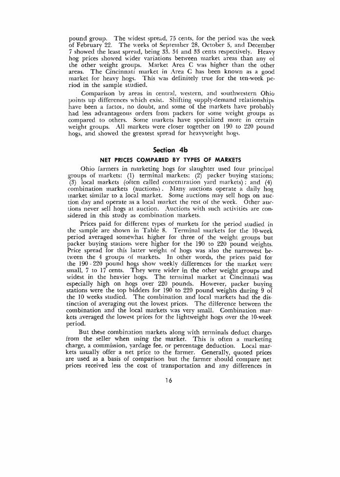
Average weekly prices for slaughter hogs by size of market are pre­~ented in Table 9. Prices for the ten-week period averaged almost the same for the different volume markets, especially for the 190 to 240 pound hogs. The difference was ~lightly wider for heavier hogs and those under I 90 pounds.

Medium size markets averaged the highest prices for the ten-week period and for most individual ·weeks by a few cents over the largest markets, but the difference was not large enough to be important. This comparison shows that volume handled per market does not bring out important differences in prices paid to farmers. Prices by areas and types of markets were more important.

Section 5 PRlCES IN SAMPLED AREA COMPARED TO SELECTED MARKETS A comparison was made oi the prices paid in sampled area and

the markets at Cincinnati, Columbus, Cleveland, Indianapolis and 85 Ohio Intetrior Markets' (Table 10). Averages for the 10-week period

1Prices are reported ) days per week bv the Ohio Department of Agriculture.

18

Table 9- Weekly Avereage Net Prices of Slaughter Hogs for Small, Medium, :md Large Volume Markets, by Four Weight Groups for a Ten-Week Penod, Ohio 1959-1960

(dollars per hundredweight)

180·190 Pounds Range of

D•tc Small MediUm Large Average Weekly Average.

Sept.l4 -18 $13.42 $13.57 $13.44 $13.48 .13 Sept.21 -25 13.53 13.72 13.55 13.60 .19 Sept. 28- Oct. 2 13.19 13.19 13.0(1 13.13 .19 Oct.5 -9 12.55 12.60 12.42 12.52 .18 Nov.16-20 12.55 12.71 12.66 12.64 .16 Nov.23-27 12.62 12.72 12.67 12.67 .10 Nov. 30- Dec. 4 12.33 12.49 12.39 12.40 .16 Dec. 7 -ll 12.35 12.45 12.37 12.39 .10 Feb. 15 -19 13.20 13.35 13.30 13.28 .15 Feb.22-26 13.47 13.67 13.61 13.58 .20

Average $12.92 $13.05 $12.94 $12.97 .13

190·220 Pounds Range of

Date Small MediUm Large Average Weekly Average

Sept. 14- 18 $13.79 .4ji13.82 ~13.79 ~13.80 .03 Sept. 21 -25 13.88 13.90 13.88 13.89 .02 Sept. 28 - Oct. 2 13.-!0 13.43 13.37 13.40 .06 Oct. 5-9 12.87 12.86 12.81 12.85 .06 Nov.16-20 12.95 12.99 12.99 12.98 .04 Nov. 23 · 27 12.99 13.02 13.00 13.00 .03 Nov. 30- Dec. 4 12.73 12.75 12.72 12.73 .03 Dec. 7 -II 12.7~ 12.69 12.60 12.67 .12 Feb.15- 19 13.55 13.60 13.56 13.57 .05 Feb.22-26 13.85 13.92 13.87 13.88 .o7 Average $13.27 $i13.30 $13.26 $13.28 .04

220·240 Pounds Range of

Date Small MediUm Large Average Weekly Average

Sept.l4 -18 $13.50 $13.59 ll!13.51 $13.53 .09 Sept.21 -25 13.59 13.66 13.61 13.62 .07 Sept. 28 - Oct. 2 13.14 13.19 13.07 13.13 .12 Oct.5 -9 12.60 12.64 12.57 12.60 .07 Nov.l6-20 12.44 12.51 12.55 12.50 .II Nov.23 ·27 12.47 12.52 12.53 12.51 .06 Nov. 30- Dec. 4 12.22 1225 12.24 12.24 .03 Dec. 7 -II 12.19 12.18 12.18 12.18 .01 Feb. 15 -19 13.24 13.26 13.28 13.26 .02 Feb.22-26 12.52 13.59 13.57 13.56 .07 Average $12.89 !j:12.94 $12.91 $12.91 .05

240·260 Pounds Range of Date Small Medium Large Average

Weekly Average

Sept. 14. 18 9)12.96 $13.03 $12.98 $12.99 .o7 Sept. 21-25 13.02 13.17 13.08 13.09 .15 Sept. 28 ·Oct. 2 12.58 12.73 12.54 12.62 .19 Oct.5 · 9 12.04 12.18 11.96 12.06 .22 Nov.16-20 11.87 11.95 12.02 IUI!I .15 Nov. 23-27 11.91 11.95 12.01 11.96 .10 Nov. 30- Dec. 4 11.63 11.67 I 1.72 11.67 .09 Dec. 7 -ll 11.53 11..'>7 11.61 11.57 .08 Feb.15 -19 12.68 12.75 12.82 12.75 .14 Feb.22 -26 13.oi 13.07 13.11 13.06 .10 Average $12.32 $12.41 $12.39 $12.37 .09

19

Table 10- Weekly A'•erage Net Prices Above and Below Ohio Sampled Area Prices for 190-220 Pound Slaughter Hogs at Cleveland, Cincinnati, Columbus, Inil:ianapolis and 85 Ohio Interior Markets During a Ten-Week Period, 1959-1960

Date

Sept.l4 -18 Sept. 21 -25 Sept. 28- Oct. 2 Oct. 5-9 Nov.16-20 Nov. 23-27 Nov. 30- Dec. 4 Dec. 7-11 Feb.l5 -19 Feb. 22-26 .\verage

Date

Sept.14 -18 Sept. 21-25 Sept. 28- Oct. 2 Oct. 5-9 Nov.l6-20 Nov.23 -27 Nov. 30- Dec. 4 Dec. 7-11 Feb.15 -19 Feb. 22-26 .\verage

(dollars per hundredweight)

Average

-~13.80 13.87 13.37 12.85 12.97 13.00 12.71 12.66 13.57 13.91

$13.27

Average

:1'13.72 13.71 13.23 12.76 12.86 12.92 12.51 12.43 13.46 13.82

:1)13.15

Sampled Area• Range

Sl3.65- 13.91 13.84. 13.90 1 3.!3- 13.65 12.64 . 13.37 12.86-13.13 12.89- 13.!0 12.62. 12.82 12.!'i0- 12.84 13.38- 13.84 13.69 - 14.20

Cmcinnati Range

:"13.57- 13.82 13.57 - 13.82 12.92- 13.75 12.42- 13.07 12.67- 13.07 12.92- 12.92 12.42- 12.57 12.02- 12.67 13.29- 13.69 13.67- 14.17

.kCmcinnati and Columbus pnces W('re POt mcludt:.d.

Date

Sept. 14-18 Sept. 21 -25 Sept. 28 -Oct. 2 Oct. 5-9 Nov.l6-20 Nov.23 ·27 Nov. 30- Dec. 4 Dec. 7-11 J:leb. 15 -19 Feb.22 -26 Average

Average

-~13.!\9 13.70 13.!9 12.70 12.9;i 13.()7 12.62 12.61 13.17 13.70

$13.13

Indianapolis Range

;11;13.36- 13.71 13.61- 13.79 12.94- 13.36 12.61 - 12.99 12.84- 13.11 12.99- 13.24 12.49-12.84 12.49-12.79 13.11-13.36 13.46- 13.91

Average

'!113.60 13.75 13.35 12.7!'i 13.05 13.13 12.85 12.8!) 13.75 14.00

$13.31

Average

$13.66 13.76 13.26 12.76 12.86 12.89 12.61 12.61 13.46 13.76

:i\13.16

Cleveland Range

:m.50-13.75 13.75- 13.75 13.25- 13.50 12.50- 13.25 13.00- 13.25 13.00- 13.25 12.75- 13.00 12.75-13.00 13.75- 13.75 13.7ii -14.25

Columbus Range

'\13.51- 13.76 13.76- 13.76 13.01-13.51 12.51- 13.26 12.76- 13.01 12.76 - 13.Dl 12.51- 12.76 12.51 - 12.76 13.26- 13.76 13.51- 14.01

85 Ohw Interior Markets A\erage

Sl3.72 13.82 13.32 12.77 12.92 12.95 12.69 12.62 13.57 13.82

$13.22

Range

Sl3.56- 13.82 13.82-13.82 13.07- 13.57 12.57 - 13.32 12.82- 13.07 12.82- 13.07 12.57- 12.82 12.57- 12.82 13.32- 13.82 13.57 -14.07

show the Cleveland market was the only one averaging higher (6 cents) than markets in the ~ampled area. Cincinnati was 12 cents lower, Co­lumbus ll cents, 85 Interior markets 5 cents; and Indianapolis 14 cents. In other words, commission. yardage and other charges have been de­ducted from quoted prices so that all prices are reasonably comparable."

For certain weeb, the price spreads were much higher than the averages (weeks December 7-ll and September 14-18). However, there was not a definite pattern for the period ~tudied. The Cleveland mar-

2Sec pages 22~23 for more complete explanation.

20

ket ~howed the wide~t variation compared to the ~ampled area lor the 190-220 pound weight hogs.

In the sampled area of southwt:><;tern Ohio, larmen received as high or higher prices for their hogs as any other area in the state except for those near the Cleveland market. In this study no considerations werv made for transportation and other costs, but livestock fanners know that the transportation costs and differences in shrink are considerable when traveling 75 miles to a market as compared to 10 or 15 miles.

Section 6 TRANSPORTATION RATES (COSTS) COMPARED TO THE PRICES PAID

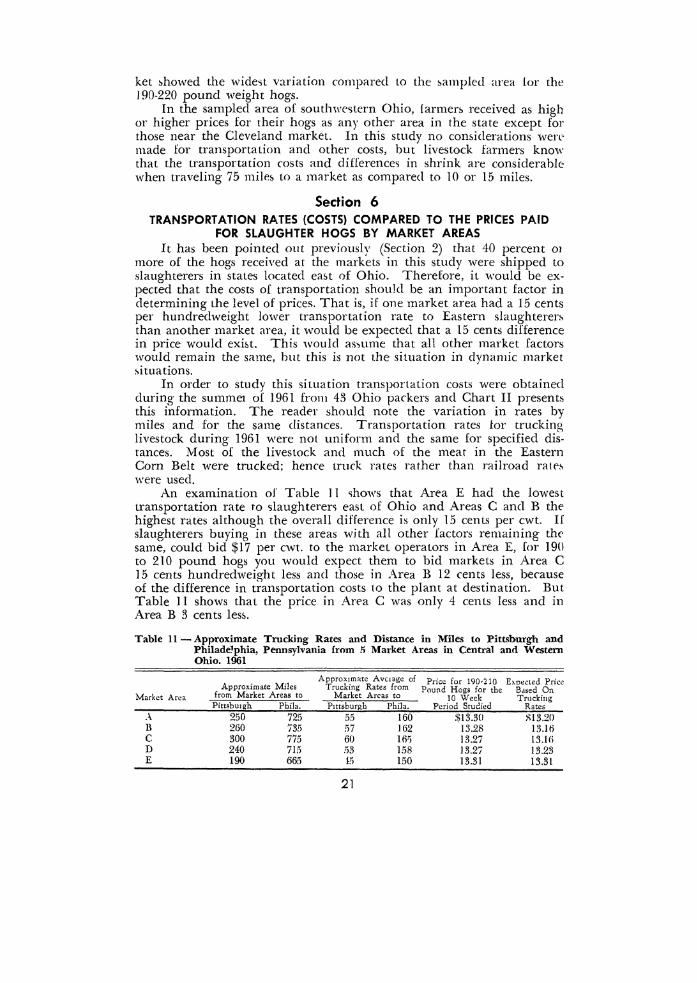
FOR SLAUGHTER HOGS BY MARKET AREAS It has been pointed out previously (Section 2) that 40 percent 01

more of the hogs received at the markets in this study were shipped to slaughterers in states located ea~t of Ohio. Therefore, it would be ex­pected that the costs of transportation should be an important factor in determining the level of prices. That is, if one market area had a 15 cents per hundredweight lower transportation rate to Eastern slaughterer~ than another market area, it would be expected that a 15 cents difference in price would exht. This would as~ume that all other market factors would remain the same, but this is not the situation in dynamic market ~i tua tions.

In order to study this situation transportation costs were obtained during the summeJ: of 1961 from 43 Ohio packers and Chart II presents this information. The reader should note the variation in rates by miles and for the same distances. Transportation rates for trucking livestock during 1961 were not uniform and the same for specified dis­tances. Most of the livestock and much of the meat in the Eastern Corn Belt were trucked; hence truck rates rather than railroad ratr~ were used.

An examination of Table II ~hows that Area E had the lowest transportation rate to ~laughteren east of Ohio and Areas C and B the highest rates although the overall difference is only 15 cents per cwt. If slaughterers buying in these areas with all other factors remaining the same, could bid $17 per cwt. to the market operators in Area E, for 190 to 210 pound hogs you would expect them to bid markets in Area C 15 cents hundredweight less ancl those in Area B 12 cents less, because of the difference in transportation costs to the plant at destination. But Table 11 shows that the price in Area C was only 4 cents less and in Area B 3 cents les~.

Table I I - Approximate Trucking Rates and Distance in Miles to Pittsburgh and Philadelphia, Pennsylvania from !'i Market Areas in Central and Western Ohio. 1961

Market Area

.\ B c D E

Approximate Miles from Market Areas to Pittsbmgh Phila.

250 725 260 735 300 775 240 715 190 665

Apprmo.matc AvClage of Price fol' 190~210 E>.pt:cted Price Truckmg Rates from Pound Hogs for the Based On

Market Areas to 10 Week Trucking Pittsburgh Phila. Period Studied Rates

5~i 160 $13.30 )1;13.20 57 162 13.28 13.Hi 60 l()'J 13.27 13.11i .">3 158 13.27 13.23 15 150 13.31 13.31

21

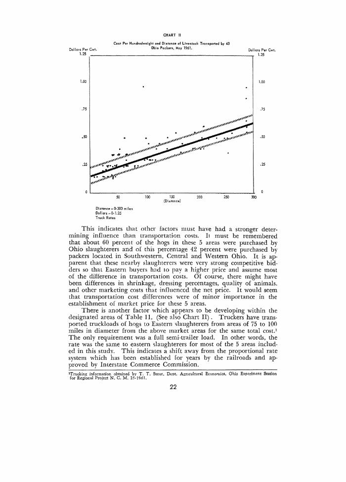
Dollars Per Cwt. 1.25

CHART II

Cost Per Hundredweight and Distance of Livestock Transported by 43 Ohio Packers, May 1961.

Dollars Per Cwt. 1.25

1.00 1.00

50

Distance- 0-300 miles

Dollars- 0-1.25 Truck Rates

100 150 (Distance)

200 250 300

This indicates that other factors must have had a stronger deter­mining influence than transportation costs. It must be remembered that about 60 percent of the hogs in these 5 areas were purchased by Ohio slaughterers and of this percentage 42 percent were purchased by packers located in Southwestern, Central and Western Ohio. It is ap­parent that these nearby slaughterers were very strong competitive bid­ders so that Eastern buyers had to pay a higher price and assume most of the difference in transportation costs. Of course, there might have been differences in shrinkage, dressing percentages, quality of animals, and other marketing costs that influenced the net price. It would seem that transportation cost differences were of minor importance in the establishment of market price for these 5 areas.

There is another factor which appears to be developing within the designated areas of Table 11, (See also Chart II) . Truckers have trans­ported truckloads of hogs to Eastern slaughterers from areas of 75 to 100 miles in diameter from the above market areas for the same total cost.l The only requirement was a full semi-tr::tiler load. In other words, the rate was the same to eastern slaughterers for most of the 5 areas includ­ed in this study. This indicates a shift away from the proportional rate system which has been established for years by the railroads and ap­proved by Interstate Commerce Commission. 'Trucking information obtained by T. T. Stout, Dept. Agncultural Economics, Ohio Experiment Station for Regional Project N. C. M. 2 5 • 1961.

22

Section 7 THE PROCEDURE IN THE ESTABLISHMENT OF THE DAILY

MARKET PRICE FOR HOGS Each market day the person responsible for the hog market must

establish a price. This price mmt be established so that the market operator can buy hogs !rom the farmer and sell them to a slaughterer with enough margin to pay expemes and have some net income remain­ing from operations. Otherwise he will soon cease to be a market operator.

A check of operations in the offices of the many men responsible for the establishment of the hog market in the Eastern Corn Belt points up the many economic facton that influence the establishment of price each market day.

Usually market operators consider their own receipts for the pre­vious week and the receipts of any other markets with which they have contact and any other information that has iniluencecl the market. Next, they consider the estimated receipts for today for their own mar­kets and the 85 Ohio markets. Thev also obtain the estimated market receipts for the major markets. Son{e check these for 9, 10, or 12 mar­kets. Much information is secured by long distance telephone conversa­tions. Market information hy wire is obtained by some firms, but this is an added cost and not all operaton use it. Most of the market op­erators keep informed on the recent day-to-day changes of the wholesale prices of hams, butts, loins, bellie~, picnics, and lard. They also ob­serve whether these products are moving easily through retail stores to the consumer (demand conditions) or slowing clown and piling up and remaining unsold in packer inventories.

Starting about 7:30 to 8.00 a.m. these market men begin to talk long distance to their many contact'> to secure the early information. The markets at Cincinnati, Indianapolis, Chicago, and St. Louis are usually included. They usually check on the rains and storms, favor­able or unfavorable weather for farm operations, (planting, seeding, harvesting, combining, etc.) or any other situation that may influence a light, normal, or heavy movement from the farms. They find out whether any market animals have been held over and they are especial­ly interested in the estimated receipts for the present market day. With this background of early information, most operators have partially decided whether the market will be steady, lower, or higher. Experi­ence in establishing the market gives them a good indication at what price the market will be established.

Market operator& are also interested in the orders of the packers for the market day. These calls are made early by most market op­erators. They exchange price information on early sales of any market that opens, whether it is steady, weak, or strong, and the amount ol change up or clown, 25 to 50 cents per hundredweight. It is always in­teresting to note that packer buyen tend to be on the weak or lower side if the market turns out to be steady with the previous market day. The market operator~ in their conver~ation tend to talk more toward a

23

steady or higher market. The p::~cken, are also concerned with the normal numbers to be slaughtered and the movement of meat the pre­vious day or days to the retailer5. 15 it moving normally for the period of the year or is it backing up with the retailers asking for concessiom in prices, etc.? They note too the changes in the wholesale prices for the primal cuts, namely, loins, butts, picnics, bellies, hams, and lard. Packers during periods of light supplies are aho concerned with their guaranteed hours and wages required per week for their labor. They desire to slaughter enough live>tO(k to meet their minimum wage re­quirements. Occasionally some may be strong buyers pricewise in or­der to get hogs and keep labor working their minimum requirements for the week.

The above information i~ exch;mged early in the day generally before 8:30 a.m. or by 9:00 a.m. The early morning radio broadcast> go out a few minutes before or just after 9:00 a.m. Usually the market is indefinite at that time, but the estimated receipts are usually well established. Sometimes the trend of the market is reasonably well in­dicated, but usually the 9:00 a.m. broadcasts in the Eastern Corn Belt are indefinite.

It is during thi5 time period that packers are making bids and giving orders, some tentative, others firm. Many packers are in contact with all kinds and types of markets including terminals, local markets, and their own packer buying station&. These early offers to buy may involve conditions which are further approved or modified by telephone calls sometime later in the morning. These changes often influence the final price established.

By 9:00 a.m. the market operators who usually establish the market are commencing to e~tablish in their own minds about what the mar­ket will be for that clay. At this point it should be remembered by the reader that there are definitely two classes of market operators in the establishment of the hog price in the Eastern Corn Belt. These are the leaders1 and the followers. There are relatively few leader~ but many followers. The followers can keep their market information costs lower. They make fewer long distance calls. They spend less for telephone, wire, and teletype services, and listen to the radio reports and establish their markets later in the morning. Some call their competitive mar­kets in their area and then establish the price for their own market or markets.

On the other hand, the leaders stay on the long distance telephone. They obtain any changes in the orders for the packers. They indicate what they believe the quoted price v:ill be in the conversations between packer buyers and market operators. Any price information on early sales for the different areas is exchanged between packer buyers, order buyers, and market operators for their selected groups. They may talk to the same persons several times for latest information.

At this stage of price determination, one group of market operators may not pass on to ;mother group what their real thinking is for the

1Some rna}· usc the term dominant firms.

24

price about to be e~tablished. On the other hand, another group ma) take an advance step~ and establish a price for example on the 190 to 220 pound weight group. These weight~ change from time to time but are illustrative. The~e early price!. may hold if the other leaders are thinking about the same. On the other hand, ii another leader group announces a different price, adjustments may be made by the first group and the followers then fall in line. Obviously there is a tremend­ou~ amount of time spent on the telephone. The long clistance tolls daily for Ohio alone would be surpri~ing to many livestock farmen, were the information available.

It is during this same period that the l\Iarket New~ Service of the Ohio Department of Agriculture is contacting many Ohio packers and market operators. The Market New~ Service obtains the estimated re­ceipts of the 9 terminal markets. They also make available the informa­tion on 85 Ohio markets. This information is given to many market operaton and others who desire the information. The l\Iarket News Service obtains the early trends and estimated number to be marketed, or other price in£luencing information including weather" and begin to estimate whether the market will be steady, higher, or lower. They obtain the actual number marketed the previous day from the market operators. The l\Iarket News Service makes return calls to see if any early sales have been made or obtain information which will give indi­cations of what the market will be:.

Early estimate~ are made and given to the newspaper pre~s services and early radio broadcasters. These are usually indications of trend. As more calls are made and the leaden have established the market, actual price quotations are established by grades and weight groups and made available to radio stations, news ~ervices, and newspapers.

Auctions are not involved in determining the price in the morning. Those auctions selling hogs usually start in the early afternoon. Prices at terminal, local markets, and packer buying stations have been estab­lished and those prices are known to the ;mction operators and to the buyers including packer buyers and order buyers. This information from the auctions are market facts which are available for use the next day by market operators.

It mu&t be remembered that this explanation is primarily for cen­tral and southwestern Ohio, but is believed with some minor variations to be approximately the same for other areas of the Eastern Com Belt.

'The market operators say "Stitk their necks out"" JWeather. such as .storm:,, unm.ual changes may influence farmcrb to move hvebtnck to market, or with, hold for a few days. Harvestin~ and other !'~nods arc important.

Section 8 PRICES FOR SELECTED WHOLESALE AND RETAIL PORK PRODUCTS IN OHIO

Changes have taken place at the production, distribution, and con­sumption levels for pork and pork products during the last 20 years in Ohio. These changes in the pork industry have been brought about largely by (1) the rapid growth of population, (2) difterent levels of consumer income, (3) consumption habits, (4) development of large

25

scale production technique~, (5) increased direct marketing, (6) decen­tralization of large wholesaling firms in the industry, (7) development of large scale retail food chains and independent supermarkets, and (8) technological developments in general.

The influence that these new developments have had upon Ohio's pork industry is of considerable intere~t to hog producers, marketing· agencies, slaughteren, retailers, and consumers. Questions asked by these groups usually arc associated with the importance and influence that these changes h:we had upon the market structure and price rela­tionships in the marketing of hogs and pork products. To provide some information that would be beneficial in answering such questions <:Jnd to acquire a more complete understanding of the pork pricing structure in Ohio, price clata from segments of the industry were ana­lyzed.

Retail Price Comparison for Selected Porh Cuts Retailers' prices are of primary interest because, changes in demand

and shifts in consumer desires are first reflected in retail prices. For this segment of the industry, data were collected by means of a tele­phone survey. This survey was conducted for an eleven-week period, beginning in September 1959, and ending in January 1960. Weekly prices for selected retail pork cuts were obtained from 48 stores of which 34 were chain stores and 14 were independent supermarkets. These stores were located in the following Ohio cities:

Number of Stores City and Population' County Chain Independent Total

800,000 and over Cincinnati Hamilton 2 2 4

300,000- 799,999 Columbus Franklin 5 2 7 Dayton l\Iontgomery 3 4

50,000 - 299,999 Hamilton Butler 3 4 Springfield Clark 3 4

10,000-49,999 Chillicothe Ross 3 4 Circleville Pickaway 3 4 Washington C. H. Fayette 4 5 Wilmington Clinton 2 3 Xenia Greene 2 3

5,000 - 9,999 Eaton Preble 2 3 Lebanon \1\Tarren 2 3

Prices involving both reguhr and special prices for selected retail cuts of pork were obtained from the sampled stores. Since most stores etablished their retail selling prices of meat on a weekly basis, prices for

1Population was based upon the metropolitan area an<d was derived from the 1960 Census of Population, U. S. Department of Commerce, Bureau of tho Census, Washington, D. C.

26

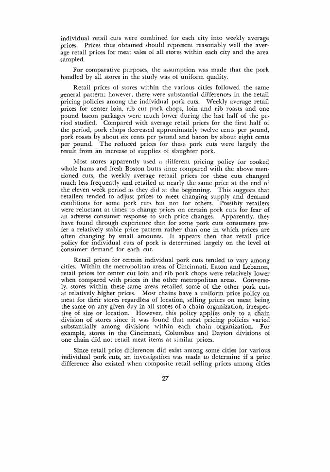
individual retail cuts were combined for each city into weekly average prices. Prices thus obtained should represent rea<;onably well the aver­age retail prices for meat <;ales of all stores within each city and the area sampled.

For comparative purpose~, the assumption was made that the pork handled by all stores in the study was oi uniform quality.

Retail prices of stores ·within the Yarious cities followed the same general pattern; however, there were substantial differences in the retail pricing policies among the individual pork cuts. \1\Teekly average retail prices for center loin, rib cut pork chops, loin and rib roasts and one pound bacon package~ were much lower during the last half of the pe­riod studied. Compared with average retail prices for the first half of the period, pork chops decreased approximately twelve cents per pound, pork roasts by about six cents per pound and bacon by about eight cents per pound. The reduced prices for these pork cuts were larg-ely the result from an increase of supplies of slaughter pork.

Most stores apparently used a diiferent pricing policy for cooked whole hams and fresh Boston butts ~ince compared with the above men­tioned cuts, the weekly average ret::tail prices for these cuts changed much less frequently and retailed at nearly the same price at the end of the eleven week period as they did at the beginning·. This suggests that retailers tended to adjust price& to meet changing supply and demand conditions for some pork cut<; but not for others. Possibly retailers were reluctant at times to change prices on certain pork cuts for fear of an adverse consumer response to wch price changes. Apparently, they have found through experience that for some pork cuts consumers pre­fer a relatively stable price pattern rather than one in which prices are often changing by small amounts. It appears then that retail price policy for individual cuts of pork is determined largely on the level of consumer demand for each cut.

Retail prices for certain individual pork cuts tended to vary among cities. Within the metropolitan areas of Cincinnati, Eaton and Lebanon, retail prices for center cut loin and rib pork chops were relatively lower when compared with prices in the other metropolitan areas. Converse­ly, stores within these same areas retailed some of the other pork cuts at relatively higher prices. Most chains have a uniform price policy on meat for their stores regardless of location, selling prices on meat being the same on any given clay in all stores of a chain organization, irrespec­tive of size or location. However, this policy applies only to a chain division of stores since it was found that meat pricing policies varied substantially among divisions within each chain organization. For example, stores in the Cincinnati, Columbus and Dayton divisions of one chain did not retail meat items at >imilar prices.

Since retail price differences did exist among some cities for various individual pork cuts, an investigation was made to determine if a price difference also existed when composite retail selling prices among cities

27

were compared (Table I 8) .~ Compari~om indicated that weeklv com­posite retail prices of pork "·ere nearly the ~ame for all citie~. The aver­age range in composite prices among cities for the sampled eleven-week period was under four cent:, per pound. Thi~ suggests that even though prices for individual pork cut~ varied among cities, little actual price difference was present when prices for the major retail cuts were com­bined into composite prices.

:!The method used i'l computing compo::ate retail and wholesale priqes was similar to the. method used by the Market News Branch, Livestock Diviston, USDA. Followinp: ..tre the costs on whtch retail prices were obtamcd and the yield or percent of carcass:

Retatl Cuts Percent Whole Ham> (cooked) 10•4#

B<tcon (cured) 8·12# P1cnics (smoked) 4·S# Center Loin Cut Pork Chops Center R1b Cut Pork Chops Loin Cut Pork Roosts Rib Cut Pork Roasts Boston Butts

Total

11.76 10 66 6.16 2.30 2.30 2.30 2.30 4. )0

Wholesale Cuts Whole Hams (cooked) 12·16#

Bocon (cured) 10·12# P1cmcs (smoked) 4·8#

Loms (fre;h) 8·12 Boston Butts (fresh)

Total

Percent

12.14 10.3; 6.31

9.4; 1.08

43.H

Less than 100 percent of the carcas5 cuts were priced. The average composite retail price per pound wa~ calculated by dividing the total value of the retail cuts by the total percent of the cuts.

28

Table 11- Weekly Average Retail Prices for Center Cut Loin Pork Chops by Cities, Ohio 1959-1960 (price in dollars per pound)

September October December January Ctty and Tov .. •n 18 25 2 ') 16 23 3 10 17 } 1 7 Average

Hamilton s .90 $ .92 $ .92 $ .91 s .89 $ .90 $ .80 $ .75 ~ .75 1' .79 :,; .79 ~ .85 Springfield .99 .95 .95 .93 .93 .9?. .84 .82 .83 .Btl .83 .89 \Vashington C. H. .92 .89 .89 .88 .87 .87 .81 .80 .82 .83 .81 .85 Xenia .98 .95 .94 .93 .93 .u~~ .R5 83 .87 .87 .85 .90

Cincinnati .92 .92 .91 .90 .89 .88 .81 .78 .79 .77 .77 .85 Dayton .99 .99 .99 .99 .96 .96 .89 .86 .89 .92 .86 .!14 Ci1.cleville .92 .90 .90 .88 .88 .88 .83 .81 .83 8" . ~ .81 .86 Eaton .98 .90 .89 .87 .87 .84 .74 .70 .70 .67 .69 .80

Chillicothe .93 .91 .91 .89 .89 .!liJ .80 .79 .82 .82 .81 .86 Lebanon .86 .82 .82 .82 .80 .80 .74 .70 .69 .68 .68 .76 Columbus .98 .96 .94 .93 .94 .94 .87 .85 .86 .88 .86 .91

Average $ .94 s .92 s .91 ;;; .90 $ .90 ::li .89 .~ .82 $ .79 $ .80 j, .80 $ .80

Range s .86· s .82- $ .82- s .82· ).; .80- 9: .80- s .74- s .70- s .69- $ .67- S .G!l-.99 .99 .99 .99 .96 .96 .89 .86 .89 .92 .86

IV -o

Table 12- Weekly Average Retail Prices for Center Cut Rib Pork Chops by Cities, Ohio, 1959-1960 (price in dollars per pound)

September October December January C1tv and Town 18 25 2 9 16 23 3 10 17 l1

--7- Average

Hamilton ;-, .90 s .86 $ .86 s .85 s .84 s .8:) )i; .67 $ .63 !f, .65 1' .70 $ .70 $ .77 Sp1 ingfie1d .84 .82 .82 .81 .82 .lll .74 .72 .73 .76 .7ti .78 \Vashington C. H. .92 .88 .79 .79 .78 .78 .72 .71 .75 .74 .71 .78 Xenia .92 .89 .89 .87 .88 .88 .80 .78 .83 .77 .79 .85

Cincin,lati .89 .87 .79 .78 .77 .81 .69 .78 .59 .6!J .69 .76 Dayton .86 .89 .89 .89 .86 .!!6 .79 .86 .79 .R6 .8~ .85 Circleville .91 .78 .85 8:'\ .86 .8'; .71 .77 .73 .70 .6H .79 Eaton .80 .76 .76 .74 .74 -<) ·'- .64 .64 .60 .62 .63 .70

Chillicothe .88 .86 .86 .85 .85 .85 .76 .75 .82 .80 .7ll .82 Lebanon .79 .77 .77 .il .68 .fill .60 57 .!)7 .56 .!lfi .66 Columbus .92 .96 .88 .87 .88 .87 .80 .78 .80 .81 .79 .85

.\\f;!ragc s .88 $ .85 $ .83 :,., .82 s .81 'li .8:? li .72 $ .73 $ .7l $ .73 $ .72

Range $ .79- $ .76· $ .76- s .71- $ .68- ~ .68- $ .60· $ .57- $ .57- $ .56- $ .55-.92 .96 .89 .89 .88 .88 .80 .86 .83 .86 .82

Table 13- Weekly Average Retail Prices for Loin Cut (price in dol1a:rs per pound)

Pork Roast by Cities, Ohio, 1959-1960

September October De<: ember January Cit\· and Town 18 25 2 9 16 23 3 10 17 H

--7- Average

Hamilton )) .61 $ .57 $ .56 s .56 $ .57 <; .56 $ .50 s .51 l) .47 $ .50 $ .50 $ .54 Sp1ingtield .55 .:)6 '" -~lO

-r. .!),_) "C. .!).) .:>-1 .51 JiO .!\0 .50 .50 .53

\Vashington C. H. .53 .52 .33 .:'>l .51 .31 .47 lfi .45 .46 .4!i .49 Xenia .56 .. )!1 .56 .53 .54 .53 .49 .47 .-16 .47 .·!i .:i 1

Cincinnati ,,j[J .58 .5i .. >5 55 "'' .. )~) .19 .59 .49 .48 AS .54 Davton .55 .56 . .'Hi .. >3 .55 .. ):J .35 . .'i3 .!i3 56 .. 'i3 "" .:J,)

Ch:cleville .55 .:14 .34 .. H .57 .:J!J 54 .47 .49 .52 .49 .53 Eaton • .'i7 .51) .54 .i'>"l .~JD .50 .49 .49 .48 .50 .-18 . .'i3

Chillicothe .53 .52 .:>3 . .'i3 53 .59 .47 .-15 .45 .45 .45 .50 Lebanon 57 .55 .55 .55 .54 .5'1 .. )() .46 .41) .46 .46 .51 Columbus .54 .53 .54 .51 .53 .56 .47 .47 .-17 .48 .48 .51

.\\t>rage 5) .56 s .55 s .55 s .54 s .54 :- .55 $ .50 s .·19 s .48 s .49 $ .48

Range _<; .53- s .52· s .:'\3- s .51- s .51- s .51- s .47- s .45- s .45- s .45- s .45-.61 .58 .57 .51) .57 .GO .35 .. )9 .53 .56 .53

w 0

Table l4- Weekly Average Retail Prices for Rib Cut Pork Roast by Cities, Ohio, 1959-1960 (price in dollars per pound.)

September October December January

City and To"U.·n 18 ~) 2 9 16 23 3 10 17 31 --7-

Average

Hamilton s .50 s .45 $ .45 s .45 s .45 s .·15 s .40 -~ .39 s .39 % .36 $ .40 !; .43 Springfield .48 .-17 .46 .47 .47 .47 .43 43 .43 .43 .43 .45 Washington C. H. .47 .46 .-16 .43 .43 .43 .39 .:l7 .37 .37 .37 .41 x~nia .47 .46 .Hi .43 .43 .-!:l .39 .:17 .37 .36 .37 .41

Cincinnati .50 .48 .48 .55 .47 Ali AI AI .38 .40 .42 .45 DaylOn .46 .-16 .47 .:\3 .47 .47 .45 .42 .47 .47 .42 .46 Cil.cleville .47 .·Hi A6 .47 .45 .. )0 .43 .40 .w .37 .37 .43 Eaton 50 .46 .47 .48 .45 Atl .40 .38 .38 .38 .31i .43

Chillico t h!' Ai .46 .46 .46 .43 .43 .39 .38 .:!8 .37 .38 .42 Lebanon .45 .44 .44 .44 .44 .43 .39 .37 .37 .36 .38 .41 Columbus .45 .44 .44 .!2 .44 .46 .40 .38 .37 .37 .38 .41

Average !; .47 s .46 $ .46 $ .47 .$ .45 ~ .45 $ .41 $ .39 $ .39 $ .39 $ .39

Range $ .45- $ .44- $ .44- $ .42- $ .43- $ .43- $ .39- .$ .37- $ .37- $ .36- $ .36-.50 .48 .48 .55 .47 .50 .45 .42 .47 .47 .43

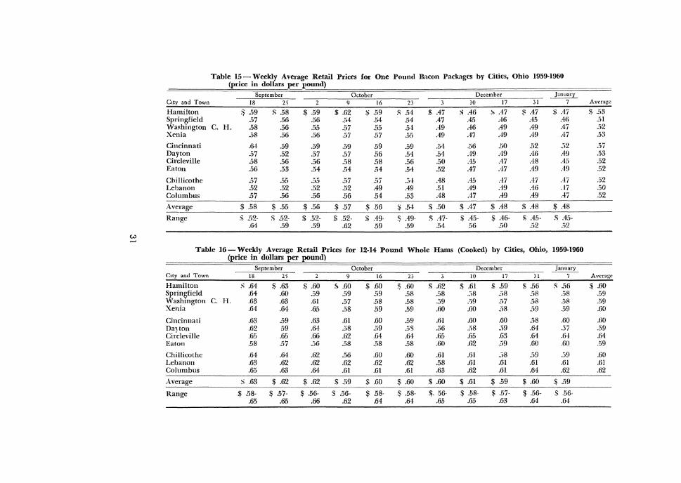
Table 15- Weekly Average Retail Prices for One Pound Bacon Packages by Cities, Ohio 1959-1960 (price in dollars per pound)

September October December January C.ty and Town 18 25 2 9 16 23 3 10 17 31

--7- Average

Hamilton ~.59 .1; .58 .$ .59 $ .62 ~ .59 j; .54 $ .47 s .46 ·" .-17 1'= .47 $ .47 * .53 Springfield .57 .56 .56 .54 .54 .54 .47 .45 .46 .45 .46 .iii Washington C. H. .58 .56 .55 .57 .55 .54 .49 .46 .49 .49 .47 .52 Xenia .58 .56 .56 .57 .57 •r,

.~}.) .49 .47 .49 .49 .47 .53

Cincinnati .64 .59 .59 .59 .59 .59 .ii4 .i\6 .50 52 .32 .57 Dayton .57 .52 .57 57 .56 .54 .54 .49 .49 .46 .49 "" .. );) Circleville .58 .56 .56 .58 .58 .56 .50 .45 .47 .48 .45 .52 Eaton .56 .53 .54 .54 M M .52 .47 .47 .49 .49 .52

Chillicothe .57 .55 .55 .57 .57 .:14 .48 .45 .47 .47 .47 .52 Lebanon .52 .52 .52 .52 .49 .49 .51 .49 .49 .46 .!7 .50 Columbus .57 .56 .56 .56 .54 .53 .48 .47 ..19 .49 .47 .52

Average $ .58 $ .55 .$ .56 $ .57 $ .56 ~.54 $.50 $ .47 $ .48 $ .48 $ .48

Range ); .52- s .52- $ .52- $ .52- $ .49· !') .49- :') .'17- $ .45- $ .46- $ .45- ~ .45-.64 .59 .59 .62 .59 .59 .54 56 .50 .52 .ii2

w ~

Table 16-Weekly Average Retail Prices for 12-14 Pound Whole Hams (Cooked) by Cities, Ohio, 1959-1960 (price in dollars per pound)

September October December January C1ty and Town 18 25 2 9 16 23 3 10 17 31 7 Average

Hamilton s .64 $ .63 s .60 ji, .60 $ .60 s;; .60 $ .62 $ .61 $.59 $ .56 s .56 $ .60 Springfield .64 .60 .59 .59 .59 .58 .r;8 .38 .58 .58 .58 .59 Washington C. H. .63 .63 .61 .57 .58 .58 . .'l!J .')9 .!i7 .58 .58 59 Xenia .64 .64 .65 .58 .59 .59 .60 .60 .58 .59 .59 .60

Cincinnati .63 .59 .63 .61 .60 .59 .61 .60 .60 .58 .60 .60 Da)ton .62 59 .64 .58 .59 .!iS .56 .58 .:19 .64 .:>7 .59 Circleville .6.1) .65 .66 .62 .64 .64 .65 .65 .63 .64 .64 .64 Eaton .58 .57 .. ;6 .58 .58 .58 .60 .62 .59 .60 .60 .!i!J

Chillicothe .64 .M .62 .56 .60 .60 .61 .151 ..)8 .59 .39 .60 Lebanon .63 .62 .62 .62 .62 .62 .58 .61 .61 .61 .61 .61 Columbus .65 .63 .64 .61 .61 .61 .63 .62 .61 .64 .62 .62

Average s .63 $ .62 $ .62 s .59 s .60 $ .60 $ .60 $ .61 $ .59 $ .60 $ .59

Range $ .58- $ .57- $ .56- s .56- s .58- .s .. ~8- !!;. 56- $ .58- $ .57- $ .56- s .56-.65 .65 .66 .62 .64 .64 .65 .65 .63 .64 .64

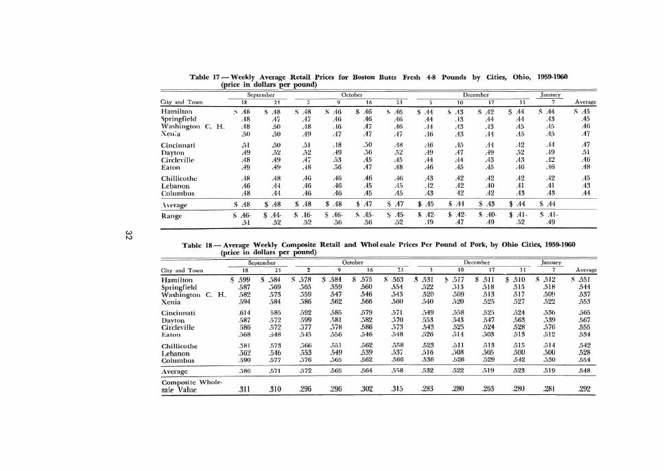
Table 17- Weekly Average Retail Prices for Boston Butts (price in dollars per pound)

Fresh 4-8 Pounds by Cities, Ohio, 1959-1960

September October December January City and Town 18 2) 2 9 16 23 3 10 17 31

--7- Average

Hamilton s .48 s .48 S AS s .16 $ .46 J'. .46 $ .44 s .43 s .42 s .44 s .44 s .45 Springfield .48 .47 .47 .46 .46 .46 .44 .H .44 .41 .43 .45 'Vashington C. H. .48 .50 .-18 .!6 .47 .46 ..!4 .43 .-13 .45 .45 .46 Xen;a .r.o .50 .49 .47 .47 .'!7 .46 .43 .44 .4!\ .45 .47

Cincinnati .iiI .50 .51 .18 .:>0 .4X .-16 A·:J .44 .-12 .44 .47 Dayton .49 .5~ .:i2 .49 .36 52 .·19 .47 .49 .52 .-19 .51 CircleYille .48 .49 .47 53 .45 .45 .·H .·14 .-!3 .43 .-12 Ali Ea10n .-19 .4!1 .!8 .56 .47 .48 .46 .45 .45 .46 .46 .48

Chillicothe .48 .48 .46 .-16 .46 .46 .43 .42 .-12 A2 .-12 .. 15 Lebanon .46 .44 .46 .46 .45 .-15 _{2 .42 .40 .41 .41 .4:1 Columbus .48 .44 .46 .46 .45 .45 .43 42 .42 .43 .43 .44

.herage $ .48 $ .48 $ .48 $ .48 ~ .47 :') .47 $ .45 ~ .44 $ .43 $.44 $ .44

Range s A6- $ .44- s .t6- s .46- j\ .45- !i .45- s .42- $ .42- s .40- $ AI- s .41-.51 .52 .52 .:)6 .56 .52 .49 .47 .49 .52 .49

w

"' Table 18- Average Weekly Composite Retail and Wholesale Prices Per Pound o[ Pork, by Ohio Cities, 1959-1960 (price in dollars per pound)

September October December January

Cit.y and Town 18 2) 2 9 16 ,_ _, l I() 17 31 7 Average

Hamilton s .599 $ .:>84 s .578 s .584 $ .575 .1> .563 ~ .531 ~ 517 $ .!ill $ .510 .1> .512 s .551 Springfield .587 .:569 .365 .559 .560 .554 .522 .. il3 .518 .515 .518 .544 \Vashington C. H. .582 .573 .:559 .547 546 .:>43 .520 .509 .513 .:>17 .509 .537 Xenia .594 .584 .:\86 .562 .566 .560 .540 .:120 .525 .527 .522 .553

Cincinnati .614 585 .592 .585 .579 .571 .549 .558 .525 .524 .536 .565 Davton .!i87 .572 .!i99 .">81 .:\82 .:>70 .553 .543 .547 .563 .339 .ti67 CiJ:cle\·ille 586 .572 .377 .371:! .586 .573 .543 .525 .524 .528 .576 """ .:J,),)

Eaton 568 .:548 .545 .556 .546 .548 .526 .514 -503 .513 .512 .534

Chillicothe .581 .573 .366 .5:)1 .562 .5!l8 .523 .:.11 .513 .515 .5H .542 Lebanon .562 .546 .553 .549 .539 .:)37 .5lli .508 .505 .500 .500 .528 Columbus .:)90 .577 .376 .305 .562 .566 .536 .1>26 .529 .542 .330 .554

Average .386 -571 .572 .565 .564 .5tJ8 .532 .!>22 519 .523 .519 .54S

Composite Whole-sale Value .311 .310 .296 .296 .302 .315 .283 .280 .263 .280 .281 .292

Section 9 SUMMARY AND CONCLUSIONS

Price relation~hips between 46 markets to which fannen sold hogs were <;tudied in this publication. These markets covered 28 counties in Central, Western, and South·western Ohio, the important hog producing area of the state. For approximately the same period, pork prices were obtained from 48 stores in 12 cities of the same area, (Cincinnati, Co­lumbus .. Dayton, and 9 other county seat cities) . Prices were obtained over a period of 10 weeks from September 14, 1959 to February 26, 1960, but were for hogs shipped between October 10 and November 15 and December l 1 to February 14.

l. Net prices paid to the farmers at the market over the 10 week pe­riod averaged almost the same for 190-220 weights for the 5 marketing areas. The price i>pread was narrowe~t on thi<; weight group and widest for the 240-260 pound hogs.

2. The widest weekly range of 75 cents between areas was for the 240-260 pound hogs during the week of February 22-26. The narrowest was 4 cents during the week of September 21-25 for the 190-220 pound hogs.

3. Prices varied between individual markets by week- periods and farmers need to keep this point in mind when marketing.

4. Terminal market prices for the period studied were highest for 180 to 190 pound, 220-240, and 240-260 pound weight groups. Packer buying stations were highest for the 190-220 pound hogs.

5. The lowest prices were paid by the combination and local mar­kets. The difference was close for all weight groups except for the lightweight hogs.

6. Size of market did not seem to be a factor in prices paid. The medium size market was highest although the difference was small.

7. Many of the markets kept the prices well in line with nearby com­petitors, but for certain days and periods substantial differences occur­reel. Some markets were observed to be relatively high for a period and then would be "in line" with other markets. Apparently unusual buying orders from packers were important factors influencing prices during periods when <;ome markets had unusually high prices.

8. It was found that this group of 46 markets handled during the 10 week period nearly ·150,000 slaughter hogs weighing from 180 to 260 pounds. Almost 57 percent were solei to packers located in Ohio. Pennsylvania and New Jersey packers were the largest out-of-state buyers taking slightly more than 28 percent of the volume. The remaining 15 percent went to 8 other states. This shows that out-of-state packers during the period studied were ~trong bidders and purchased more than 40 percent of the volume handled by the 46 markets. Packers located in Central and Southwestern Ohio, as would be expected, purchased the largest percentage of hogs going to Ohio packers.

9. Prices received by farmers in the sampled area for the 10 week period received as high or higher prices for their 190-220 pound hogs than any other area in the ~tate except for farmers near Cleveland. Fanners more distant would have to consider differences in transporta­tion costs.

33

10. Almost all hogs were tramported by truck to packers from the markets in this study. Prices between nearby markets were reasonably close, thereby preventing inter-market trucking. However, farmers rea­~onably close to two or more markets may shift sales to the higher mar· ket. This tends to keep the markets reasonably close with respect tu price.

II. Since most of the hogs ~old to out of the state slaughteren were transported to Pennsylvania and Ne·w Jersey, it was found that market Area E had the lowest trucking rate to Pittsburgh and Philadelphia. Based on the averages paid truckers by slaughterers, the trucking rate for hogs was l5c per hundredweight highe1 for the Cincinnati area com­pared to Columbus, and if the difference in transportation cost were considered, the expected price would be 15 cents per hundredweight lower in market Area C. Actually it was only 4 cents lower. Apparent­ly slaughterers buying in these areas as~ume some of the extra trucking cost.

12. There seems to be a different trucking rate ~tructure developing. Railroad rates increa"e every 10 to 20 miles in the area east of the Mi&­sissippi River, but in Ohio some trucker~ were charging the same rate in areas 75 to 100 miles in diameter. provided they have full semi-trailer loads. This pattern of rates, should it become permanent, could defi­nitely influence the price pattern and standard in western Ohio for hogs.

13. The 48 retail ~tores, during the 10 week period studied, dropped rib pork chops 17 cents per pound, loin chops 14 cents, and 1 pound ot bacon 10 cents compared to $1,20 drop per hundredweight in live hog prices. At the same time whole h'ims dropped only 4 cents per pound and Boston butts 5 cents. Prices varied between cities as would be ex­pected, but as supplies increa5ed and live hog prices dropped, retail prices followed.

14. In studying retail and whole~ale pork prices it wa& found general­ly that a higher relatiomhip existed when retail prices were compared one week later (a one week lag). This points out that retail prices normally were adjusted one week later than wholesale, or that pork buyers for retail stores purchased their pork supplies one week in ad­vance of sales.

34

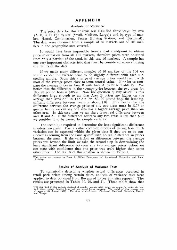
APPENDIX

Analysis of Variance'

The price data for this analysis was classified three ways: by area (A, B, C, D, E) ; by size (Small, l\Jedium, Large) ; and by type of mar­

ket, (Local, Combination, Packer Bulying Station, and Terminal) . The data were obtained from a sample of 46 markets out of 104 mar­kets in the geographic area covered.

It would have been impossible from a cost standpoint to obtain price information from all 104 markets, therefore prices were obtained from only a portion of the total, in this case 46 markets. A sample ha~ one very important characteristic that must be considered when studying the results of the data.

If we made many different samples of 46 markets of the I 04 we would expect the average price to he s1ightly different with each suc­ceeding sample. From this a range of average prices would result with most of the average prices close to bome central value. Now let us com­pare the average prices in Area B with Area A (refer to Table 2). We notice that the difference in the average price between the two areas for 180-190 pound hogs is $.0386. Now the question quicky arises: Is this difference large enough to say that Area B prices are higher on the average than Area A? In Table 2 for 180-190 pound hogs the least sig­nificant difference between means is about $.07. This means that the difference between the average price of any two areas must be $.07 or greater before we can say one area has a higher average price than an­other area. In this case then we say there is no real difference between area B and A. If the difference between any two areas is less than $.07 we consider it to be caused by sample variation.

The technique required to determine the least significant difference involves two parts. First a rather complex process of testing how much variation can be expected within the given data if they are to be con· sidered as coming from the same system with no real difference in prices between the areas. If the variation, or difference between the average prices was beyond the limit we take the second step in detennining the least significant difference between any two average prices before we can state with confidence that one price was truly higher than some other price. The results of this analysis is shown in Table I. 'This section was prepared bv Ed~ar A. Miller, Department of Agricultural Eoonomics and Rural

Sociology.

Results of Analysis of Variance Tests To statistically determine whether actual differences occurred in

retail pork prices among certain cities, analysis of variance tests were applied to data obtained from Bureau of Labor Statistics reports.' The results are presented in Tables 19, 20, and 21. These tables show that

'The data used in this analysis consisted of moMhlv average retail priocs per pound for center cut loin pork chops, cooked (whole) hams and one pound bacon packages. The period of time covered was six years (1954 through 1959). The cities involved were: Cincinnati, Cleveland, Columbus, Detroit and Chicago.

35

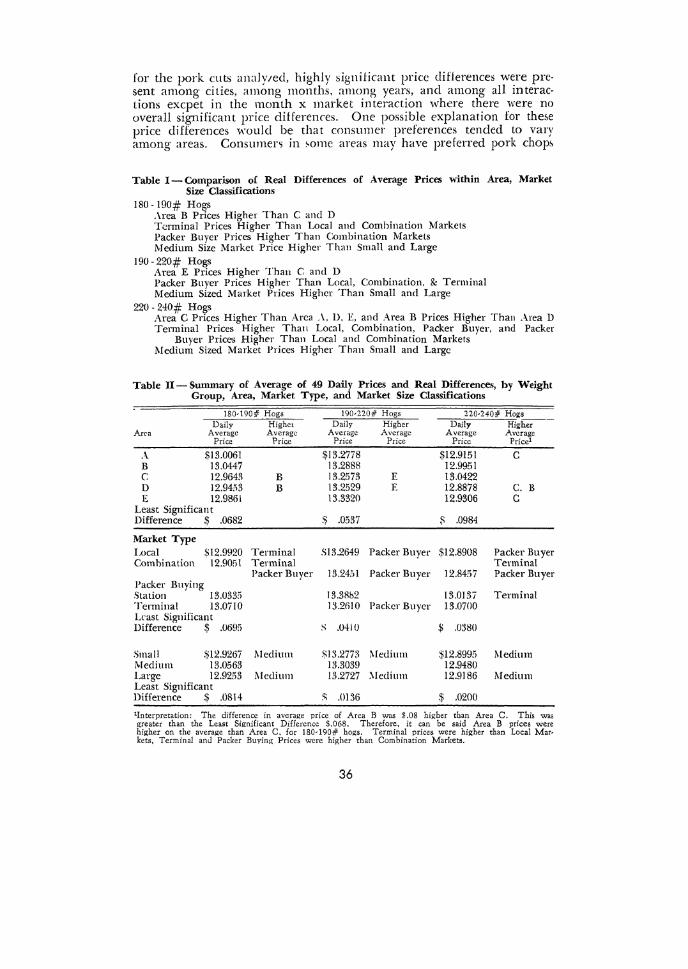
for the pork cuts analy1ed, highly significant price diflerences were pre­sent among cities, among months, among years, and among all in terac­tions excpet in the month x market interaction where there were no overall significant price differences. One possible explanation for these price differences would be that consumer preferences tended to vary among areas. Consumers in 'omc areas may have preferred pork chop'

Table I-Comparison of Real Differences of Average Prices within Area, Market Size Classifications

180-190# Hogs . \rea B Prices Higher Than C and D T.::rminal Prices Higher Than Local and Combination Markets Packer Buyer Prices Higher Than Combination Markets Medium Size Market Price Higher Than Small and Large

190- 220# Hogs Area E Prices Higher Than C and D Packer Buyer Prices Higher Than Local, Combination. & Terminal Medium Sized Market Prices Higher Than Small and Large

220- 240# Hogs Area C Prices Higher Than Area . \, D. E, and Area B Prices Higher Than ,\rea D Terminal Prices Higher Than Local, Combination, Packer Buyer. and Packer

Buyer Prices Higher Than Local and Combination Markets Medium Sized Market !'rices Higher Than Small and Large

Table II-Summary of Average of 49 Daily Prices and Real Differences, by Weight Group, Area, Market Type, and Market Size Classifications

180•190# Hogs 190-220# Hogs 220·240# Hogs Daily Highet Daily Higher Daily Hig~-

An: a Average Average Average Average Average Average Price Price Price Price Price Price1

A $13.0061 $13.2778 .$12.9151 c B 13.0447 13.2888 12.9951 c 12.9643 B 13.2573 E 13.0422 D 12.94a3 B 13.2529 E 12.8878 c. B E 12.9861 13.3320 12.9306 c

Least Significant Difference .$ .0682 $ .0537 :j; .0984

Market Type Local $12.9920 Terminal :'513.2649 Packer Buyer $12.8908 Packer Buyer Combination I2.90al Terminal Terminal

Packer Buyer 13.24!,1 Packer Buyer 12.8457 Packer Buyer Packer Buying Station 13.033!> 13.3Rb2 13.0137 Terminal Terminal 13.0710 13.2610 Packer Buyer 13.0700 Least Significant Difference $ .069!\ s .0410 $ .0380

Small $12.9267 l\ledium .)13.277!1 :\ledium $12.8995 Medium Medium 13.0563 1!1.3039 12.9480 Large 12.9253 Least Significant

Medium 13.2727 :\ledium 12.9186 Medium

Difference $ .0814 s .0136 $ .0200

11nterpretation: The difference in average price of Area B was $.08 higher than Area C. This was greater than the Least Significant Difference $.068. Therefore, it can be said Area B prices were higher on the average than Area C. for 180•190# hogs. Terminal prices were higher than Local Mar· kets, Terminal anJ Packer Buving Prices were higher than Combination Markets.

36

(.)

'-I

Table 19-Rerults of Analysis of Variance Tests of Differences in Average Monthly Retail Prices per Pound for Center Cut Loin Pork Chops at Cleveland, Columbus, Cincinnati, Detroit, and Chicago, 1954·1959

Factors _-

88 DF MSS F 5% 1% Total 2.1903 359 .00610111 Market .1038 4 .02595000 67.802846 3.41 2.41 Month .7896 ll .07178182 187.55343 2.34 1.83 Year .7406 3 .14812000 387.Qll848 :lll 2.26 i\Ion th x l\f arket .0156 H .00035456 .926366 1.69 1.45 Year x Market .0435 20 .00217500 :>.682897 1.97 1.62 MonthxYear .4130 55 .00750909 19.619951 1.62 1.42 Error .0842 220 .00038273

Table 20-Results of 4nalysis of Variance Tests of Difference& in Average Monthly Retail Prices per Pound for Whole Hams (cooked) at Cleveland, Columbus, Cincinnati, Detroit and Chicago, 1954-1959

Factors 88 DF MSS F '% 1% Total .9217 359 .00256741 Market .1813 4 .00453250 22.357623 3.41 2.41 l\Ionth .0568 ll .00516364 25.470852 2.34 1.83 Year .4677 3 .00935400 46.1 !0807 3.11 2.26 Month x Marlet .fll43 44 .00032500 1.693139 l.69 1.45 Year x Market .0300 20 .00150000 7.399103 !.97 1.62 Month x Year .1270 55 .00230909 11.390135 1.62 1.42 Error .0446 220 .00020273

Table 21- Results of Analysis of Variance Tests of Differences in Average Monthly Retail Prices for One Pound Bacon Pack­ages at Cleveland, Columbus, Cincinnati, Detroit, and Chicago, 1954-1959

Factors 88 DF MSS F ;% 1%

Total 3.7327 359 .01039749 Market .3216 4 .08040000 336.914290 3.41 2.41 Month .2659 11 .02417273 101.295238 2.34 1.83 Year 2.3842 3 .47684000 1998.186697 3.11 2.26 Month x Market .0162 44 .00036818 1.742857 1.69 1.45 Year x Market .0671 20 .00335500 14.059047 1.97 1.62 Month x:Year .6252 55 .01136727 47.634286 1.62 1.42 Ennr .0525 220 .00023864

over pork roasts while in other areas roasts may have been preferred over chops. In other areas ham may have had the greatest acceptance, etc. Thus, these differences in preference probably had a substantial influence upon the pricing policies of food organintions.

CORRELATION ANALYSIS BETWEEN THE WHOLESALE AND RETAIL PRICES OF SELECTED PORK CUTS

Additional study into price relationships between wholesale and retail pork products were obtained by statistically comparing the re· sponses in these prices over time. To make such comparisons a personal observation schedule1 "'as used in obtaining weekly retail price data for six selected pork cuts in 29 Columbus stores over the last 20 weeks for the years 1954-1955. Average weekly wholesale values for these same pork items and for the ~arne time period were derived from the National Provisioner Daily Market Service "yellow sheets."2 To determine the relationships between these prices, a limited amount of statistical analy­sis by means of simple correlation was performed. In computing these prices, retail prices were compared with wholesale values with no lag, a one week lag and a two week lag in prices. This is a procedure of matching current average weekly retail prires with concurrent average weekly wholesale prices, with wholesale prices one week earlier and with wholesale prices two weeks earlier. The results of such analyses are presented in Table 22.

This table shows that, generally, for the various pork cuts, a stronger relationship existed between retail and wholesale prices when retail prices were Jagged one week. This suggests that most retail stores in Columbus established their retail prices to the consumer based on pur· chases from slaughterers one week in advance.

It appears that the~e stores used a different pricing policy for fresh and cured pork products. Significant relationship was found between wholesale and retail prices for fresh pork cuts in 1954-56 and 59, but not for cured pork cuts. Conversely. for the years I 957-58, a strong relationship existed between these prices for cured pork cuts, but not for fresh cut~. In 1955, a significant relationship was found between retail and wholesale prices for all pork cuts.

It became somewhat difficult to explain the irregular behavior in the relationship between wholesale :md retail prices for the various pork cuts over this period. However, it appears that when live hog prices were relatively high in the last quarter of the year, little relation­ship existed between wholesale ancl retail prices for fresh pork pro· ducts. Conversely. a high degree of relationship existed between the prices for processed or cured pork products for the same period. When live hog prices were relatively low in the last quarter of the year, sig· nificant relationship between wholesale and retail prices for fresh pork cuts is evident, but not for cured pork products.• 1The interviewer entered the meat dep'artment of eoch store weekly (primarily on Friday) and personally observed and recorded the selling prices labeled on the various meat cuts. Little or no additional information was obtained from any individuals employed by the stores.

"The choice was made because of the wide ooveragc that this source enjoys in the meat industry and considered sufficicntlly reliable for purposes of this study.

"Additional information may he obtained in Ph.D. Disoertation, Ohio Statr University. 1960. by James H. Lewis.

38

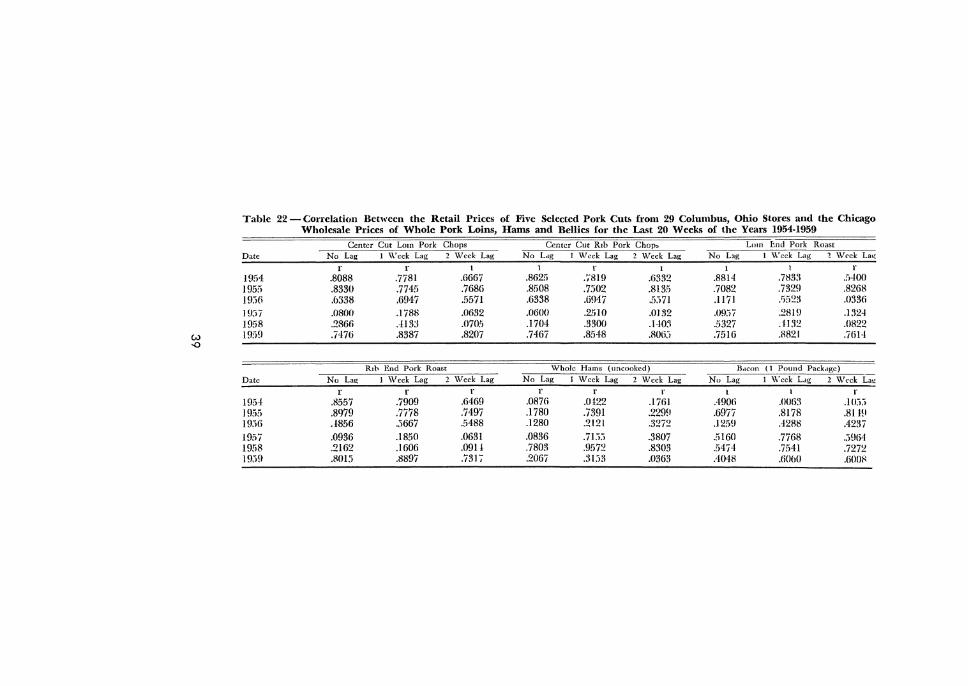
Table 22 - Correlation Between the Retail Prices of Five Selected Pork Cut& from 29 Columbus, Ohio Stores and the Chicago Wholesale Prices of Whole Pork Loins, Hams and Bellies for the Last 20 Weeks of the Years 1954-1959

Center Cut Low Pork Chops Center Cut R1b Pork Chop, Lmn End Pork Roast Date No Lag 1 \\7 cek Lag 2 Week Lag No Ldg 1 \Veck Lag 2 Week Lag No Lag I \\"cek Lag 1 \Vcck Lag

r r I l r l l l r HI 54 .8088 .7781 .6667 .86211 .7819 .6332 .8814 .7H3:l 5-100 1955 .8330 .7745 .7686 .8508 .7502 .8l3!i .7082 .7329 .8268 19.)6 .6338 .6947 .5571 ,()338 .6947 .5.171 .1171 /J52H .0336

l!l:i7 .0800 .1788 .0632 .0600 .2510 .0132 .09.>7 .2819 .132-1 1958 .2866 .-113:J .()705 .1704 .3300 .1403 .5327 .1132 .0822

w l!J£\!1 .7·17fj .8387 .8207 .7467 .8548 .BOll:> .75IG .ll821 .76H -.()

Rtb End Pork Roast Whole Hams (uncooked) Bdcon ( 1 Pound Packnge)

Date No Lag I Week Lag 2 Week Lag No Lag I Week Lag 2 Week Lag No Lag I Week L.1g 2 Week Lac

r r r r r r l l r 1954 .K557 .7909 .6469 .0876 .0122 .1761 .4906 .OOti:l .I OJ.i 1955 .8979 .7778 .7497 .1780 .7391 .2299 .6977 .8178 .811!1 19.'ili .!856 .5667 .5488 .1280 .2121 .3272 .1259 .-12fl8 A237

1957 .0936 .1850 .0631 .0836 .71.'\.'i .3807 .5160 .7768 .:>964 1958 .2162 .1606 .091! .7803 .9572 .8303 .5474 .7541 .727!! 19.)9 .8015 .8897 ./317 .20(}/ .:ll.J3 .0363 .4<HB .60h0 .6008