Embed Size (px)
Citation preview
An Analysis of the Demand for Western Rock Lobster
A report prepared for the Western Australian Department of Fisheries
2015.
Economic Research Associates Pty Ltd
A.B.N 90 009 383 173
97 Broadway
Nedlands WA 6009
Phone: +61 8 9386 2464
Email: [email protected]
Web Page: www.econsresearch.com
2
Introduction Western Rock lobster is the most important commercial fishery in Australia. Although the major
destinations and product format have changed over time, since the advent of refrigeration the
product has had a dominant export orientation. Most recently, exports of live lobster to China have
become the main market. Live lobster exports to mainland China are subject to a number of barriers,
so the bulk of the exports to mainland China have taken place through third party destinations. For a
long period, Hong Kong was dominant as a third party destination. More recently, Vietnam has been
the preferred location. Similar arrangements are used by other lobster exporters, including exports
of Southern Rock lobster from South Australia, Victoria and Tasmania. New Zealand Southern Rock
lobster also used these locations until recently. However, the commencement of the NZ-China free
trade agreement has resulted in almost all New Zealand Southern Rock exports going direct to
mainland China. Without a free trade agreement, other major exports such as the USA continue to
operate through the third party locations.
This paper presents an analysis of recent trends in prices and volumes for lobster exports to the
China market. The focus is on understanding how prices and volume are related for lobster, and how
demand drivers in China have influenced prices over time. The primary interest is Western Rock
lobster, but as the evidence suggests that lobster from various jurisdictions compete with each
other, the analysis also takes account of exports of Southern Rock lobster from Australia and New
Zealand as well as exports of lobster from the United States to China.
The export market is the focus because, as shown below, the export price drives the beach price.
The Market for Rock Lobster Evidence suggests that lobster species are substitutes for each other, although the degree of
substitutability between species varies.
The focus in this study is the China export market, which is where most Australian lobster go, and in
recent years, where a significant amount of North American exports also go.
The scope of the global lobster market
Various statistical studies have confirmed the general substitutability of lobster. A recent study used
cointegration analysis to tested the price relationship across lobster exports to China from Australian
states (Norman-López et al. 2014). Cointegration analysis allows for price differences between
species to be maintained, and tests whether prices generally move together while maintaining the
species price relativity over time. Lobster from each State were found to be substitutes for the other
(Norman-López et al. 2014).
Support for this conclusion is also found in the analysis of price links in the fish supply chain in
Canada (Gordon 2011). This study investigated the demand for sole and lobster species based on the
estimated high price elasticity of demand and concluded that assuming a constant price is most
appropriate for modelling lobster exports.
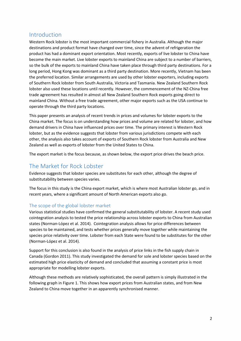
Although these methods are relatively sophisticated, the overall pattern is simply illustrated in the
following graph in Figure 1. This shows how export prices from Australian states, and from New
Zealand to China move together in an apparently synchronised manner.
3
Figure 1 Monthly trend in export prices to Greater China from Western Australia, South Australia A, &
New Zealand
Source: Prices derived from value and volume data in Australian Bureau of Statistics International Trade Customised
Report and Statistics NZ. Harmonized Trade Exports.
Notwithstanding that lobster export volumes to China from Australia and the rest of the world have
been increasing,1 there is an upward price trend for both Southern and Western Rock lobster. The
price for US exports is stable despite the large volume increase in US exports. China’s growth has
been able to absorb the extra volume.
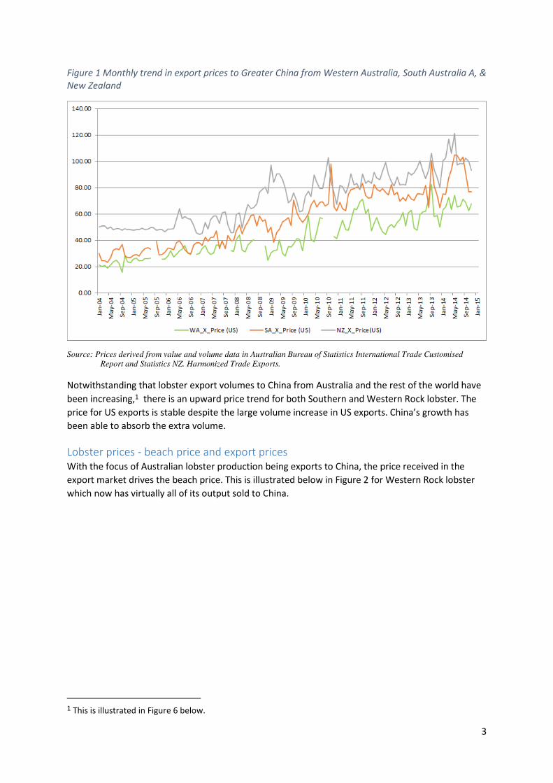
Lobster prices - beach price and export prices
With the focus of Australian lobster production being exports to China, the price received in the
export market drives the beach price. This is illustrated below in Figure 2 for Western Rock lobster
which now has virtually all of its output sold to China.
1 This is illustrated in Figure 6 below.
4
Figure 2 Beach price and export prices for Western Rock Lobster
Source; Department of Fisheries and Australian Bureau of Statistics. International Trade Customised Report.
Changes to the Management of Western Rock Lobster
The switch from an effort-controlled fishery to a quota-managed fishery fundamentally changed the
way that the market for Western Rock lobster operates.
In 2009/2010, the Government determined that the industry would move to an ITQ system
commencing with a 5500 tonnes annual quota. This quota can be varied through an annual quota
setting process. Prior to this, the fishery had been managed with effort controls where pot license
reductions were used periodically to offset “effort creep”.
The switch also enabled a change in the basic economic operation of the market. Under the effort-
controlled regime, fishers had a seven to eight month season commencing in mid-November, during
which time fishers tried to catch as much product as they could with the pots they owned. Catch
delivered to processors reflected fisher effort, and varied significantly on a daily basis. Processors
had the challenge of marketing these fluctuating catches for the best prices achievable. Since the
introduction of quota based management, fishers know the aggregate allowable catch and their
individual quotas. Processors have a greater ability to influence daily catch landed through the beach
prices they offer on a daily basis.
The significance of this change in management regime means that the time series post quota is the
most appropriate period to assess current market outcomes. This data is used in the following
analysis.
5
A Model of the Market for Western Rock Lobster
Context
Under the new quota based management system for the Western Rock Lobster Fishery, the level at
which the TACC is set for each fishing season fixes the supply of lobster for the forthcoming year. In
setting the TACC for the following fishing season, one, but only one of several considerations to take
into account is what impact, if any; would a change in the level of the TACC have on average beach
prices next season, all other things being the same? To rephrase this question, relative to the
projected average beach price next season if there was no change in the TACC, what would next
season’s projected average beach price be if the TACC did change?
Inter alia, the consequences for future beach prices of a change to the following season’s TACC will
depend on the price responsiveness of the demand curve for Western Rock lobster. However, any
assessment of price changes also needs to take account of likely shifts in demand over time due to
exogenous factors that are independent of the level of the TACC. For instance, if exogenous factors,
such as population growth and rising living standards in export markets, as well as the price of
substitute products in these markets, change between the current fishing season and the following
fishing season, then the demand for exports of Western Rock lobster will shift over time.
Short run and long run price responsiveness
It is a widely accepted fact that the time frame for buyers to adjust to a change in supply is a critical
determinant of price responsiveness because the extent to which purchasers are able to adjust their
usage of the product will depend on the length of time that they have to do so.
In the long run, there are no constraints to prevent buyers from purchasing as much or as little as
they want of a product and its substitutes. Expectations, as well as any contractual arrangements,
can be adjusted fully to the changed conditions of supply. For instance, in a long run measured in
months or even years, buyers will have plenty of time to adjust their plans. They could adjust the
quantum of substitute products purchased, and therefore will be willing to pay relatively more for an
increase in supply that is foreseen months in advance. As a result, demand will be much more
elastic, and will result in a much smaller fall in the price in response to the same increase in supply.
By contrast, there will be many constraints limiting changes to purchasing decisions in the short run,
so price changes in response to a change in supply will be much greater. In the very short run (e.g.
on a day to day basis), demand will be highly inelastic, so that an unanticipated small increase in
supply is likely to cause a substantial fall in the price in order to clear the market.
6
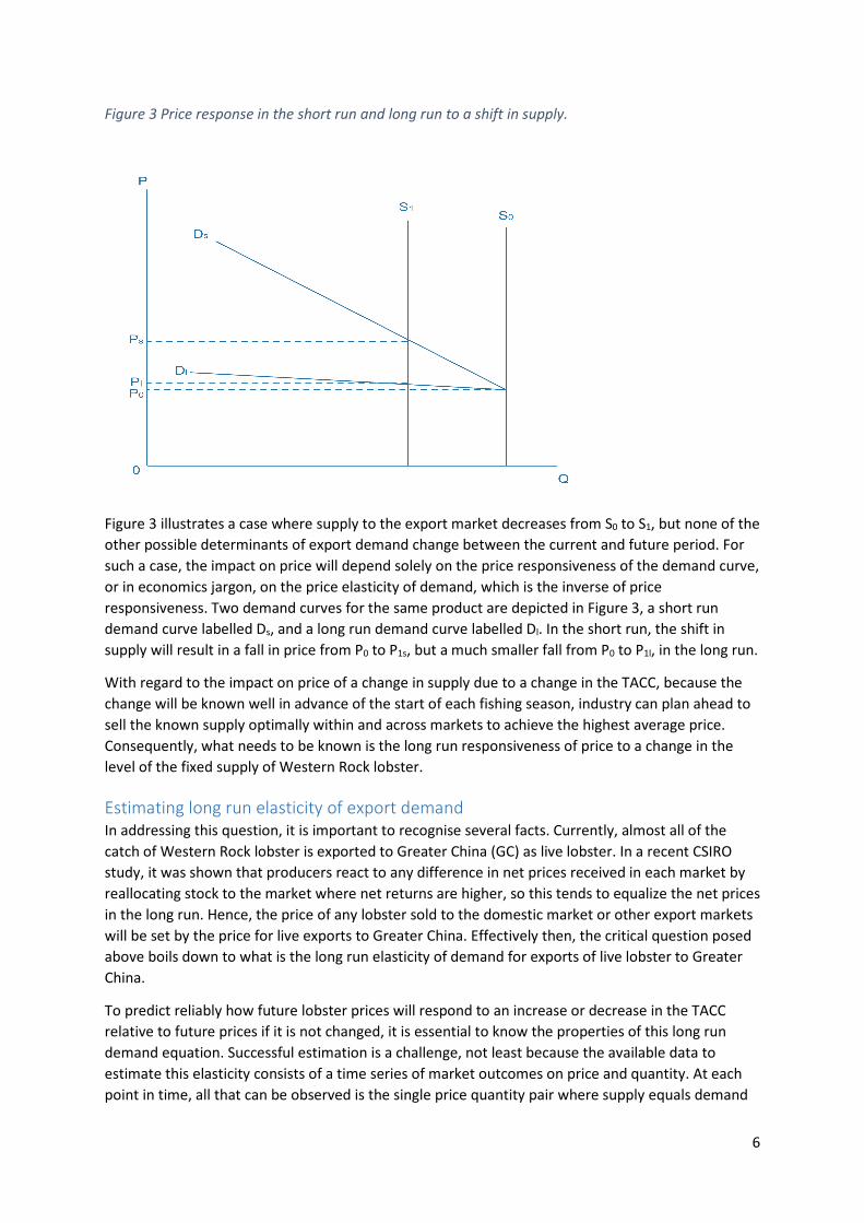
Figure 3 Price response in the short run and long run to a shift in supply.
Figure 3 illustrates a case where supply to the export market decreases from S0 to S1, but none of the
other possible determinants of export demand change between the current and future period. For
such a case, the impact on price will depend solely on the price responsiveness of the demand curve,
or in economics jargon, on the price elasticity of demand, which is the inverse of price
responsiveness. Two demand curves for the same product are depicted in Figure 3, a short run
demand curve labelled Ds, and a long run demand curve labelled Dl. In the short run, the shift in
supply will result in a fall in price from P0 to P1s, but a much smaller fall from P0 to P1l, in the long run.
With regard to the impact on price of a change in supply due to a change in the TACC, because the
change will be known well in advance of the start of each fishing season, industry can plan ahead to
sell the known supply optimally within and across markets to achieve the highest average price.
Consequently, what needs to be known is the long run responsiveness of price to a change in the
level of the fixed supply of Western Rock lobster.
Estimating long run elasticity of export demand
In addressing this question, it is important to recognise several facts. Currently, almost all of the
catch of Western Rock lobster is exported to Greater China (GC) as live lobster. In a recent CSIRO
study, it was shown that producers react to any difference in net prices received in each market by
reallocating stock to the market where net returns are higher, so this tends to equalize the net prices
in the long run. Hence, the price of any lobster sold to the domestic market or other export markets
will be set by the price for live exports to Greater China. Effectively then, the critical question posed
above boils down to what is the long run elasticity of demand for exports of live lobster to Greater
China.
To predict reliably how future lobster prices will respond to an increase or decrease in the TACC
relative to future prices if it is not changed, it is essential to know the properties of this long run
demand equation. Successful estimation is a challenge, not least because the available data to
estimate this elasticity consists of a time series of market outcomes on price and quantity. At each
point in time, all that can be observed is the single price quantity pair where supply equals demand
7
on the particular position of the demand curve at that point in time. As both the demand and supply
curves are likely to shift over time, so a time series of observations of price and quantity will almost
certainly not map different points on a single demand curve.
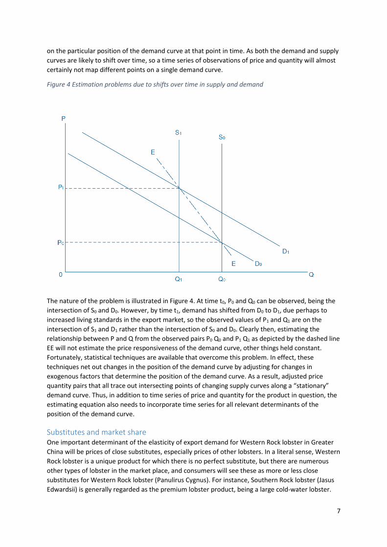
Figure 4 Estimation problems due to shifts over time in supply and demand
The nature of the problem is illustrated in Figure 4. At time t0, P0 and Q0 can be observed, being the
intersection of S0 and D0. However, by time t1, demand has shifted from D0 to D1, due perhaps to
increased living standards in the export market, so the observed values of P1 and Q1 are on the
intersection of S1 and D1 rather than the intersection of S0 and D0. Clearly then, estimating the
relationship between P and Q from the observed pairs P0 Q0 and P1 Q1 as depicted by the dashed line
EE will not estimate the price responsiveness of the demand curve, other things held constant.
Fortunately, statistical techniques are available that overcome this problem. In effect, these
techniques net out changes in the position of the demand curve by adjusting for changes in
exogenous factors that determine the position of the demand curve. As a result, adjusted price
quantity pairs that all trace out intersecting points of changing supply curves along a “stationary”
demand curve. Thus, in addition to time series of price and quantity for the product in question, the
estimating equation also needs to incorporate time series for all relevant determinants of the
position of the demand curve.
Substitutes and market share
One important determinant of the elasticity of export demand for Western Rock lobster in Greater
China will be prices of close substitutes, especially prices of other lobsters. In a literal sense, Western
Rock lobster is a unique product for which there is no perfect substitute, but there are numerous
other types of lobster in the market place, and consumers will see these as more or less close
substitutes for Western Rock lobster (Panulirus Cygnus). For instance, Southern Rock lobster (Jasus
Edwardsii) is generally regarded as the premium lobster product, being a large cold-water lobster.
8
Market prices confirm that at least some consumers prefer Southern Rock lobster to Western Rock
lobster. On the other hand, Western Rock lobster also is regarded as a premium product with taste
and size advantages compared to other lobsters from countries like South Africa, Indonesia and
Mexico, as well as Homarus spp. from North America, all of which are regarded as inferior
substitutes, and trade at a discount to Western Rock lobster. Nevertheless, the latter are purchased
in lieu of Western Rock lobster when the price of the latter is perceived to be too high relative to
other lobsters. Conversely, any fall in the relative price for Western Rock lobster will cause previous
consumers of other lobster to swap to buying Western Rock lobster instead. An important issue is
whether these various lobster products are close or distant substitutes.
If they were not substitutes at all, then an increase in the price of one would not switch demand
toward the others, but if they are close substitutes, then an increase in the price of one will cause a
switch in demand to the others as substitutes, and will trigger an increase in their price. Hence, we
can think of there being an equilibrium price structure encompassing relative prices that reflects the
various quality attributes of the lobster. In particular, a price shock in one type of lobster will be
transmitted to demand for other lobsters, so in the long run, their equilibrium relative prices will be
restored. If products are very close substitutes, then apart from the margin, effectively there will be
a price for a single product. Previous studies, as well as further analysis described below, clearly
demonstrate that most other types of lobster exported to Greater China from a number of sources
are in fact close substitutes for Western Rock lobster.
This fact is important because it means exports of Western Rock lobster from Western Australia to
Greater China make up only a small fraction of the total competing supply of lobster to this market.
Thus, at any price the export demand for WRL is equal to the amount by which total demand for
lobster in Greater China exceeds the supply of lobster from other sources of supply from around the
world.
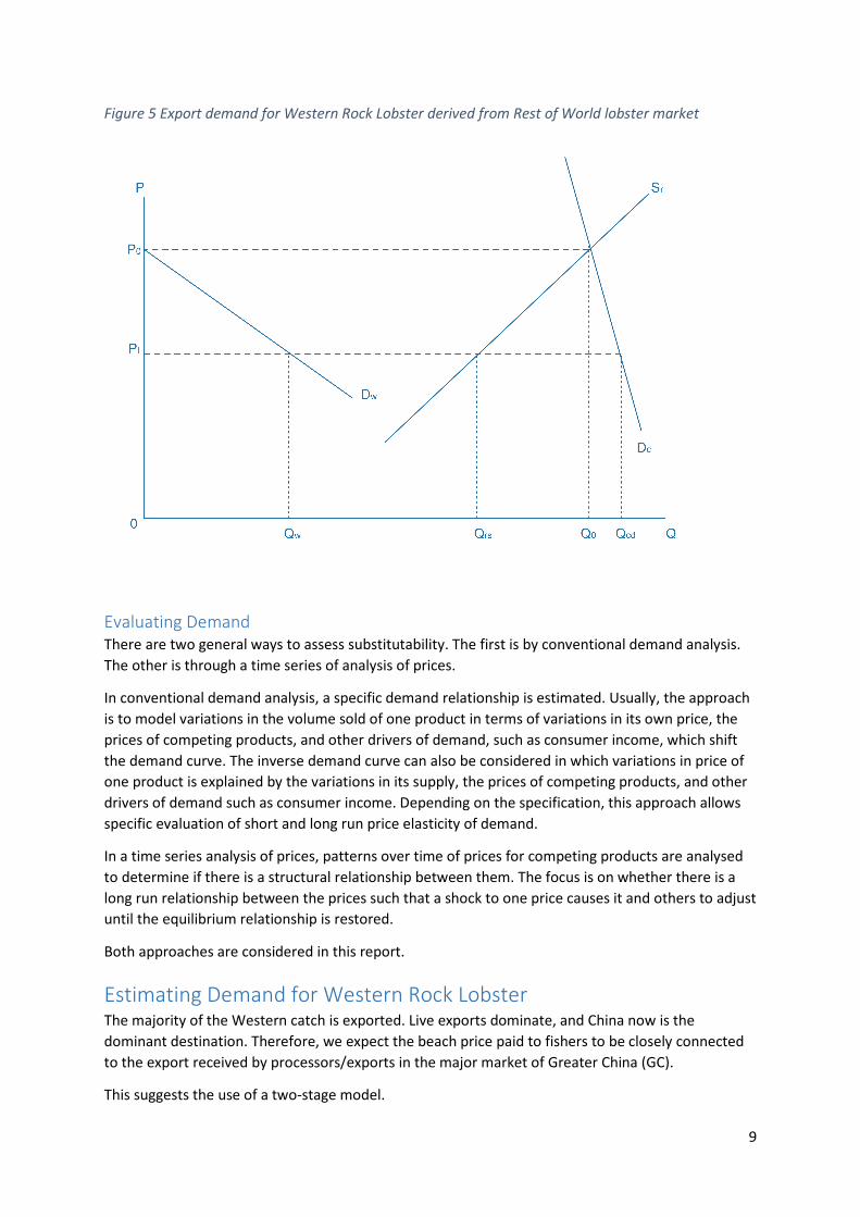
This is illustrated in Figure 5. The chart on the left hand side depicts total demand in Greater China
for lobster, and the supply to Greater China of lobster from the rest of the world (ROW i.e. all
sources other than Western Australia). The WA export demand curve depicted in the chart on the
right hand side of Figure 5 is derived by deducting ROW supply from total Greater China demand
shown in the chart on the left hand side. Note that any long run price responsiveness for WRL
exports due to a change in supply is mitigated first by the fact that WA exports make up only a small
fraction of total lobster supply to Greater China, and second by ROW supply response to any change
in price in the Greater China market. In other words, any change in the supply of WRL will in the long
run have only a small percentage impact on export prices.
9
Figure 5 Export demand for Western Rock Lobster derived from Rest of World lobster market
Evaluating Demand
There are two general ways to assess substitutability. The first is by conventional demand analysis.
The other is through a time series of analysis of prices.
In conventional demand analysis, a specific demand relationship is estimated. Usually, the approach
is to model variations in the volume sold of one product in terms of variations in its own price, the
prices of competing products, and other drivers of demand, such as consumer income, which shift
the demand curve. The inverse demand curve can also be considered in which variations in price of
one product is explained by the variations in its supply, the prices of competing products, and other
drivers of demand such as consumer income. Depending on the specification, this approach allows
specific evaluation of short and long run price elasticity of demand.
In a time series analysis of prices, patterns over time of prices for competing products are analysed
to determine if there is a structural relationship between them. The focus is on whether there is a
long run relationship between the prices such that a shock to one price causes it and others to adjust
until the equilibrium relationship is restored.
Both approaches are considered in this report.
Estimating Demand for Western Rock Lobster The majority of the Western catch is exported. Live exports dominate, and China now is the
dominant destination. Therefore, we expect the beach price paid to fishers to be closely connected
to the export received by processors/exports in the major market of Greater China (GC).
This suggests the use of a two-stage model.
10
First, we can model the export market to Greater China using an inverse demand curve of the form:
( , , , , )xw chxw xnz xsa xusP f V P P P I= (1)
where
export price for Western Rocklobster
= export volume for Western Rocklobster
=export price for New Zealand Southern Rocklobster
=export price for South Australian Southern Rocklobster
xw
xw
xnz
xsa
P
V
P
P
P
=
export price for US lobster
= income/purchaing power in China
xus
chI
=
The beach price can then be modelled as a price derived from the export price received by
processors/exporters.
( )bw xwP f P= (2)
Equation 1 models the export price received for Western Rock lobster as a function of the volume of
Western Rock lobster placed into the export market, and the prices of potential competitors such as
exports of Southern Rock lobster from New Zealand as well as from South Australia, and exports of
US lobster.
In recent times, real incomes in China have experienced strong growth. This drives growth in
demand for all consumer goods, including high-end food products like lobster. In these
circumstances, the income elasticity of demand for lobster in China may be high, perhaps greater
than one. This driver will tend to increase per capita consumption of lobster. As real incomes grow,
consumer participation in the lobster market is also likely to grow. Combined, these changes will
shift the demand curve for lobster in China to the right. All other things equal, this will tend to push
up export prices received in China over time. Note though that if suppliers increase supply to China
sufficiently, this could offset the potential price increase associated with demand growth, or even
cause prices to fall.
Equation 2 models the beach price paid as a function of the export price received.
Specific functional forms for each equation, the significance of individual variables, and the presence
of lagged effects, need to be tested with the general model framework.
Data
Data on Australian exports of live lobster are available from the ABS on a monthly basis by State and
by destination. Prices are fob in AUD. Data also is available from NZ Statistics on live lobster export
by destination. Prices are fob in NZD. Equivalent data is available on US export from the US Statistics
Agency. Prices are fob in USD. All prices were converted to USD to enable comparability and
consistent analysis.
Chinese macroeconomic data on a monthly basis is limited. The best indicator of demand growth
needs to be chosen from available measures. In this study, the monthly data on consumer goods
expenditure in urban areas is used as a proxy for spending power/incomes.
Monthly data has been assembled for Jan 2004 to Nov 2014. During 2010-2011, there was a partial
ban on exports of lobster from Australia to China, so the market was arguably not fully functional at
11
this time. Since 2009/2010, the Western Rock lobster industry has moved to quota, and the duration
of the fishing season has been extended significantly. The period Nov 2010 to Nov 2014 is therefore
the most relevant period for the analysis, as it corresponds to the current management regime.
Exports to Greater China
Exports to Greater China (GC) have been growing strongly in recent years. For the purpose of this
report, exports to Greater China include not only direct exports to China per se, but also include
indirect exports via Hong Kong and Vietnam. The quality of data on overall exports to Greater China
is patchy, but is good for some of the main sources, including West Australia, South Australia, and
the USA.
In the UN Commtrade database, worldwide exports of all types of lobster in 2013 is reported as
being 396,483 t, of which 135,375 t was rock lobster (i.e. Panulirus spp. & Jasus spp.), with the rest
being Homarus spp.. At the premium end of the market, Australia supplied 17,388 t of rock lobster
exports, and New Zealand supplied 6,276 t. The data in the Commtrade database is much less
informative in terms of the initial destination of these exports, let alone their ultimate destination.
For instance, of the 17,388 t of rock lobster exports from Australia, only 8,036 t is recorded as being
destined for Greater China ( including exports via Hong Kong, Macau, and Vietnam), while 8,694 t
has no attributed destination.
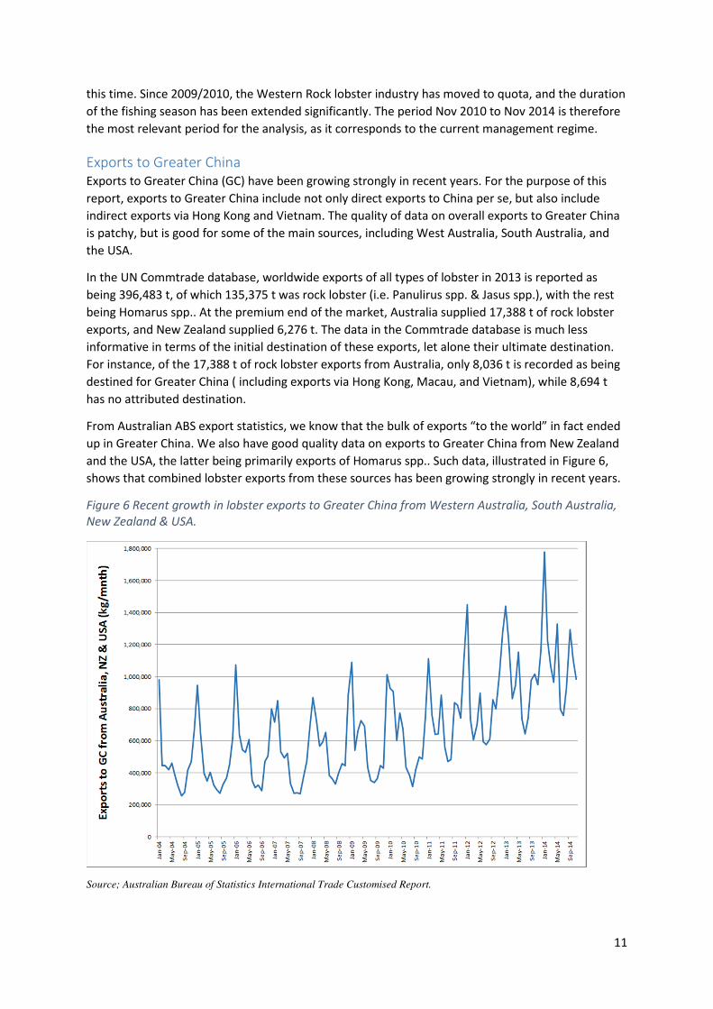
From Australian ABS export statistics, we know that the bulk of exports “to the world” in fact ended
up in Greater China. We also have good quality data on exports to Greater China from New Zealand
and the USA, the latter being primarily exports of Homarus spp.. Such data, illustrated in Figure 6,
shows that combined lobster exports from these sources has been growing strongly in recent years.
Figure 6 Recent growth in lobster exports to Greater China from Western Australia, South Australia,
New Zealand & USA.
Source; Australian Bureau of Statistics International Trade Customised Report.
12
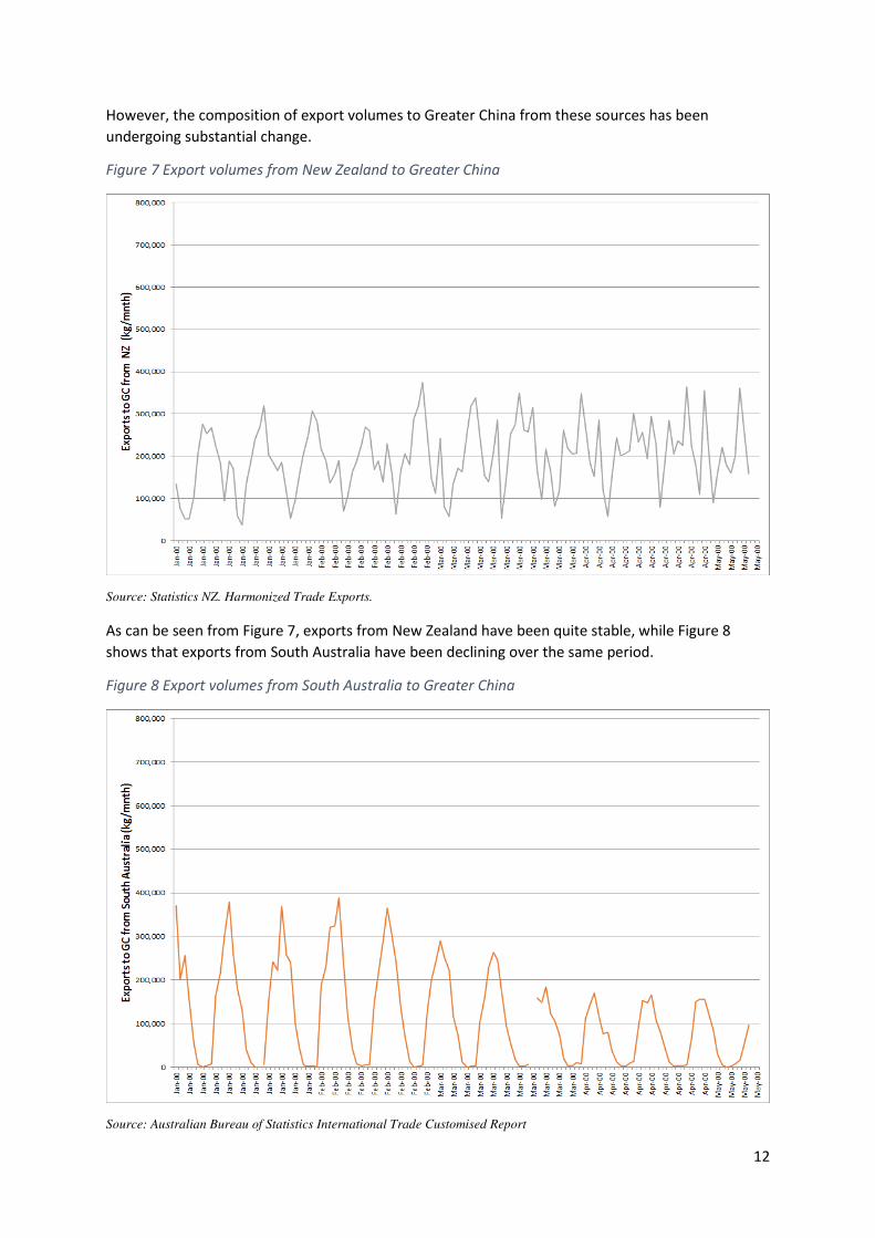
However, the composition of export volumes to Greater China from these sources has been
undergoing substantial change.
Figure 7 Export volumes from New Zealand to Greater China
Source: Statistics NZ. Harmonized Trade Exports.
As can be seen from Figure 7, exports from New Zealand have been quite stable, while Figure 8
shows that exports from South Australia have been declining over the same period.
Figure 8 Export volumes from South Australia to Greater China
Source: Australian Bureau of Statistics International Trade Customised Report
13
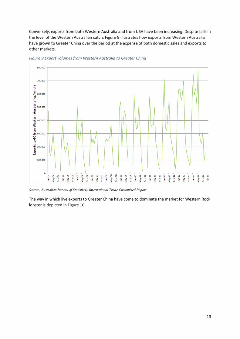
Conversely, exports from both Western Australia and from USA have been increasing. Despite falls in
the level of the Western Australian catch, Figure 9 illustrates how exports from Western Australia
have grown to Greater China over the period at the expense of both domestic sales and exports to
other markets.
Figure 9 Export volumes from Western Australia to Greater China
Source; Australian Bureau of Statistics). International Trade Customised Report
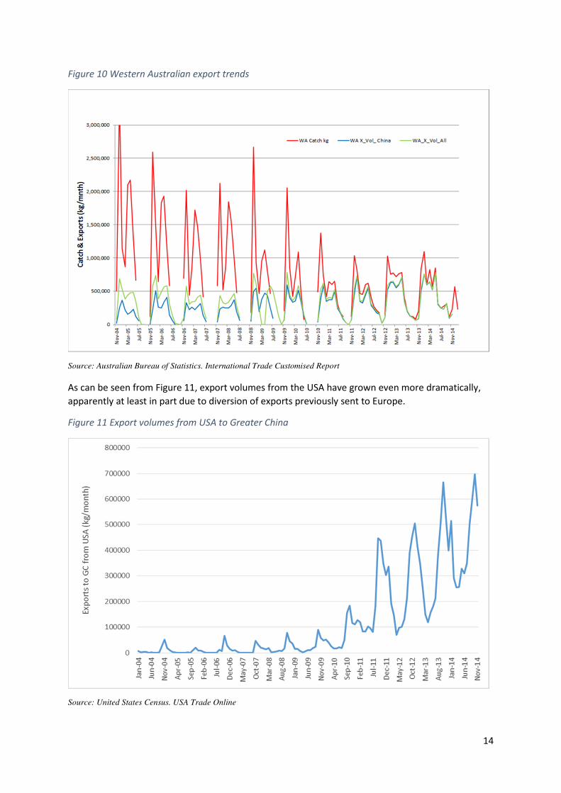
The way in which live exports to Greater China have come to dominate the market for Western Rock
lobster is depicted in Figure 10
14
Figure 10 Western Australian export trends
Source: Australian Bureau of Statistics. International Trade Customised Report
As can be seen from Figure 11, export volumes from the USA have grown even more dramatically,
apparently at least in part due to diversion of exports previously sent to Europe.
Figure 11 Export volumes from USA to Greater China
Source: United States Census. USA Trade Online
15
Apart from the above sources, exports of tropical rock lobsters from Asia, the Americas, Africa and
the Middle East along with exports of Homarus spp. from Canada, probably account for almost all of
the other lobster exports to Greater China, but in absence of reliable data, it is not possible to
document this.
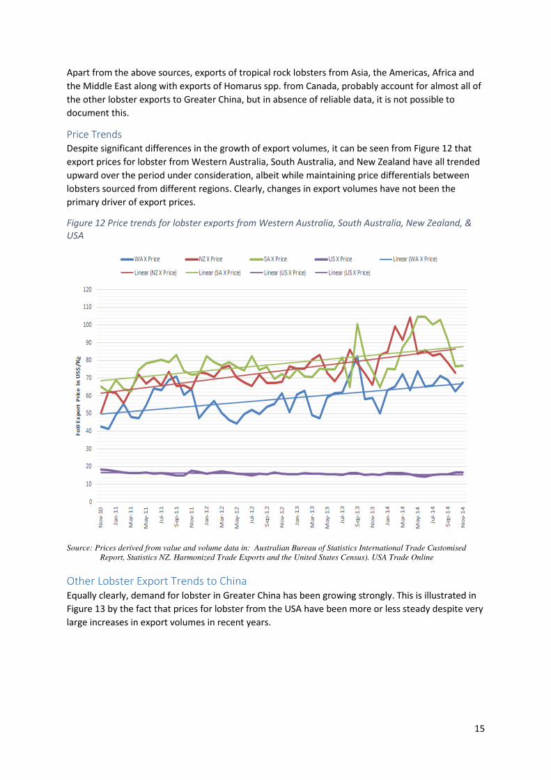
Price Trends
Despite significant differences in the growth of export volumes, it can be seen from Figure 12 that
export prices for lobster from Western Australia, South Australia, and New Zealand have all trended
upward over the period under consideration, albeit while maintaining price differentials between
lobsters sourced from different regions. Clearly, changes in export volumes have not been the
primary driver of export prices.
Figure 12 Price trends for lobster exports from Western Australia, South Australia, New Zealand, &
USA
Source: Prices derived from value and volume data in: Australian Bureau of Statistics International Trade Customised
Report, Statistics NZ. Harmonized Trade Exports and the United States Census). USA Trade Online
Other Lobster Export Trends to China
Equally clearly, demand for lobster in Greater China has been growing strongly. This is illustrated in
Figure 13 by the fact that prices for lobster from the USA have been more or less steady despite very
large increases in export volumes in recent years.
16
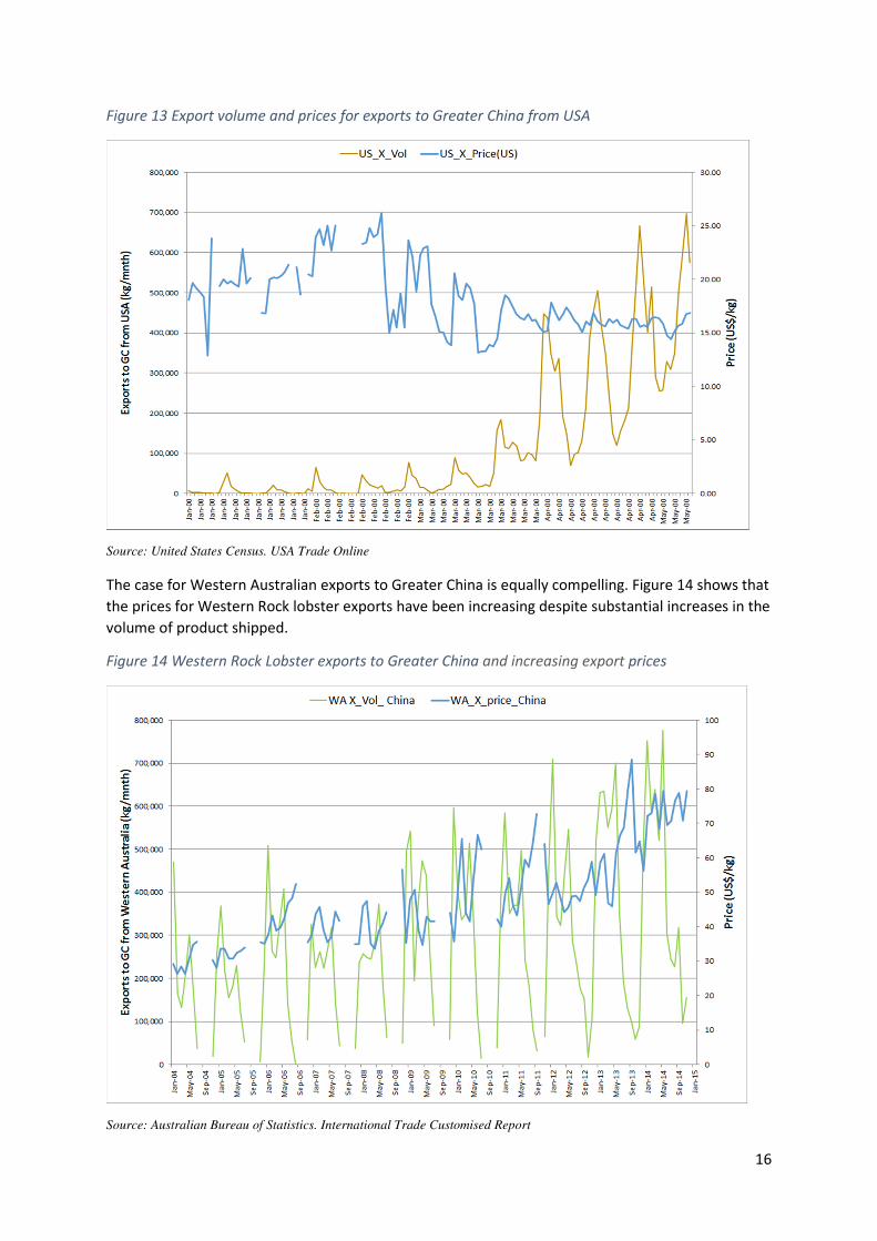
Figure 13 Export volume and prices for exports to Greater China from USA
Source: United States Census. USA Trade Online
The case for Western Australian exports to Greater China is equally compelling. Figure 14 shows that
the prices for Western Rock lobster exports have been increasing despite substantial increases in the
volume of product shipped.
Figure 14 Western Rock Lobster exports to Greater China and increasing export prices
Source: Australian Bureau of Statistics. International Trade Customised Report

17
Revenue from Exports
Figure 15 shows revenue for exports to greater China over the period since 2014. Noticeably, the
revenue from US exports increased over the period when exports were increasing strongly,
indicating that the price impact was proportionately less than the volume increase. Similarly,
revenue from Western Australian exports increased over the period when exports to China were
increasing.
Figure 15 Export revenue for exports from Western Australia, South Australia, New Zealand and USA
to Greater China ( $US).
What has Driven Prices? –Demand in China Growing Faster than Supply
The inverse demand model requires that drivers of price other than volume be included. These
drivers are variables that shift demand up or down at any given price. Typically, these variables
relate to changes in income and wealth and to changes in preferences. For example, if household
wealth is growing, or individual real incomes are growing, this may push up demand for rock lobster
at any given price. If household and individual preferences were to shift away from rock lobster, this
would push the demand down at any given price. The former would ultimately put upward price
pressure into the lobster market, whereas the latter would put downward price pressure into the
lobster market.
For the current analysis, the most obvious consideration is China’s economic growth and the
associated growth in real incomes and wealth. This has been high in China but in regions like
Shanghai, a major lobster export market, growth has exceeded that for most of the rest of China.
Monthly data on consumption and incomes in China is limited. Monthly regional data or city area
data is virtually non-existent. Data from the China National Bureau of Statistics on retail sales of
urban consumer goods was taken as a proxy for growing consumption expenditure and incomes.
0
100,000,000
200,000,000
300,000,000
400,000,000
500,000,000
600,000,000
700,000,000
2004 2005 2006 2007 2008 2009 2010 2011 2012 2013 2014
U.S. rev WA Rev SA rev NZ rev
18
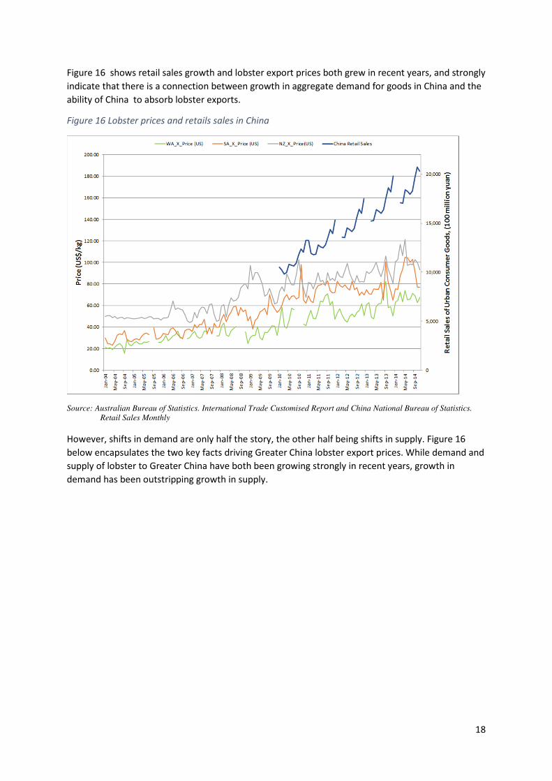
Figure 16 shows retail sales growth and lobster export prices both grew in recent years, and strongly
indicate that there is a connection between growth in aggregate demand for goods in China and the
ability of China to absorb lobster exports.
Figure 16 Lobster prices and retails sales in China
Source: Australian Bureau of Statistics. International Trade Customised Report and China National Bureau of Statistics.
Retail Sales Monthly
However, shifts in demand are only half the story, the other half being shifts in supply. Figure 16
below encapsulates the two key facts driving Greater China lobster export prices. While demand and
supply of lobster to Greater China have both been growing strongly in recent years, growth in
demand has been outstripping growth in supply.
19
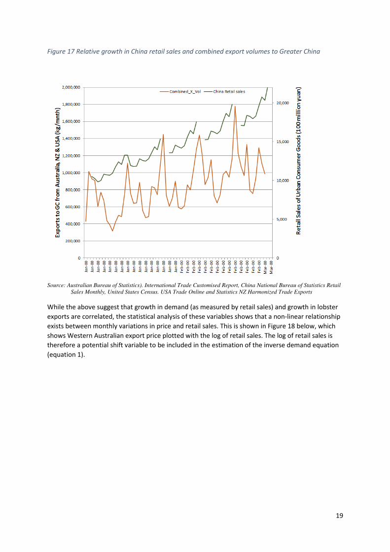
Figure 17 Relative growth in China retail sales and combined export volumes to Greater China
Source: Australian Bureau of Statistics). International Trade Customised Report, China National Bureau of Statistics Retail
Sales Monthly, United States Census. USA Trade Online and Statistics NZ Harmonized Trade Exports
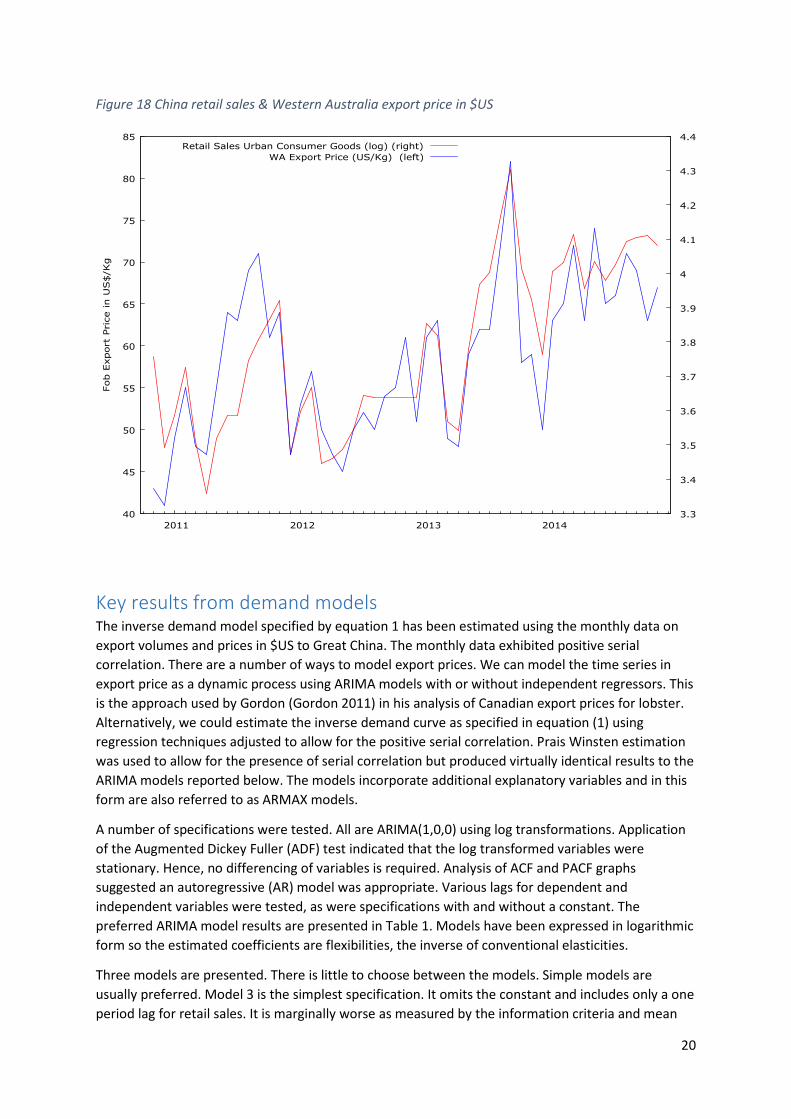
While the above suggest that growth in demand (as measured by retail sales) and growth in lobster
exports are correlated, the statistical analysis of these variables shows that a non-linear relationship
exists between monthly variations in price and retail sales. This is shown in Figure 18 below, which
shows Western Australian export price plotted with the log of retail sales. The log of retail sales is
therefore a potential shift variable to be included in the estimation of the inverse demand equation
(equation 1).
20
Figure 18 China retail sales & Western Australia export price in $US
Key results from demand models The inverse demand model specified by equation 1 has been estimated using the monthly data on
export volumes and prices in $US to Great China. The monthly data exhibited positive serial
correlation. There are a number of ways to model export prices. We can model the time series in
export price as a dynamic process using ARIMA models with or without independent regressors. This
is the approach used by Gordon (Gordon 2011) in his analysis of Canadian export prices for lobster.
Alternatively, we could estimate the inverse demand curve as specified in equation (1) using
regression techniques adjusted to allow for the positive serial correlation. Prais Winsten estimation
was used to allow for the presence of serial correlation but produced virtually identical results to the
ARIMA models reported below. The models incorporate additional explanatory variables and in this
form are also referred to as ARMAX models.
A number of specifications were tested. All are ARIMA(1,0,0) using log transformations. Application
of the Augmented Dickey Fuller (ADF) test indicated that the log transformed variables were
stationary. Hence, no differencing of variables is required. Analysis of ACF and PACF graphs
suggested an autoregressive (AR) model was appropriate. Various lags for dependent and
independent variables were tested, as were specifications with and without a constant. The
preferred ARIMA model results are presented in Table 1. Models have been expressed in logarithmic
form so the estimated coefficients are flexibilities, the inverse of conventional elasticities.
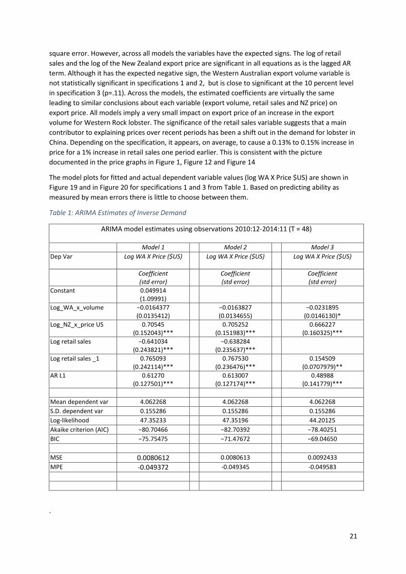
Three models are presented. There is little to choose between the models. Simple models are
usually preferred. Model 3 is the simplest specification. It omits the constant and includes only a one
period lag for retail sales. It is marginally worse as measured by the information criteria and mean
40
45
50
55
60
65
70
75
80
85
2011 2012 2013 2014
3.3
3.4
3.5
3.6
3.7
3.8
3.9
4
4.1
4.2
4.3
4.4
Fob E
xport
Price in U
S$/Kg
Retail Sales Urban Consumer Goods (log) (right)
WA Export Price (US/Kg) (left)
21
square error. However, across all models the variables have the expected signs. The log of retail
sales and the log of the New Zealand export price are significant in all equations as is the lagged AR
term. Although it has the expected negative sign, the Western Australian export volume variable is
not statistically significant in specifications 1 and 2, but is close to significant at the 10 percent level
in specification 3 (p=.11). Across the models, the estimated coefficients are virtually the same
leading to similar conclusions about each variable (export volume, retail sales and NZ price) on
export price. All models imply a very small impact on export price of an increase in the export
volume for Western Rock lobster. The significance of the retail sales variable suggests that a main
contributor to explaining prices over recent periods has been a shift out in the demand for lobster in
China. Depending on the specification, it appears, on average, to cause a 0.13% to 0.15% increase in
price for a 1% increase in retail sales one period earlier. This is consistent with the picture
documented in the price graphs in Figure 1, Figure 12 and Figure 14
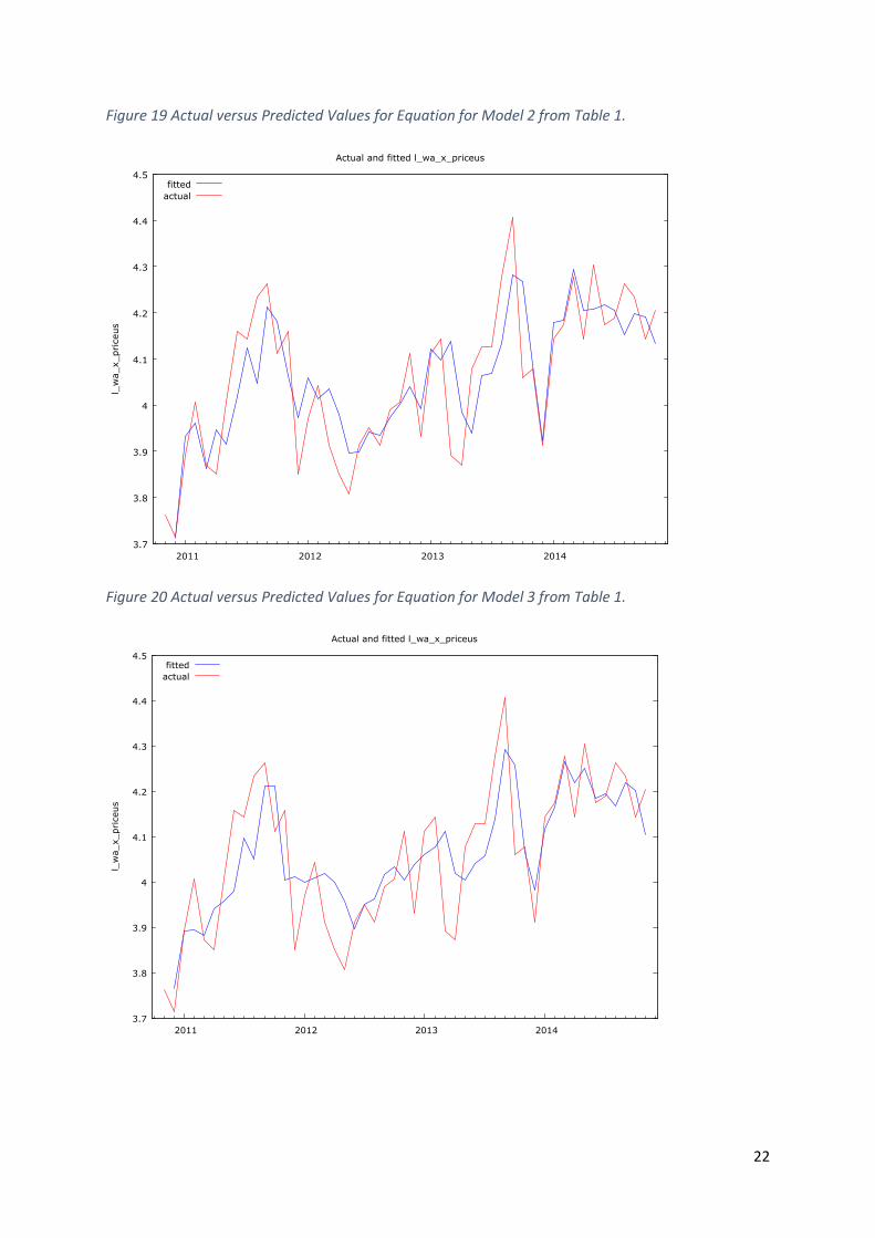
The model plots for fitted and actual dependent variable values (log WA X Price $US) are shown in
Figure 19 and in Figure 20 for specifications 1 and 3 from Table 1. Based on predicting ability as
measured by mean errors there is little to choose between them.
Table 1: ARIMA Estimates of Inverse Demand
ARIMA model estimates using observations 2010:12-2014:11 (T = 48)
Model 1 Model 2 Model 3
Dep Var Log WA X Price ($US) Log WA X Price ($US)
Log WA X Price ($US)
Coefficient
(std error)
Coefficient
(std error)
Coefficient
(std error)
Constant 0.049914
(1.09991)
Log_WA_x_volume −0.0164377
(0.0135412)
−0.0163827
(0.0134655)
−0.0231895
(0.0146130)*
Log_NZ_x_price US 0.70545
(0.152043)***
0.705252
(0.151983)***
0.666227
(0.160325)***
Log retail sales −0.641034
(0.243821)***
−0.638284
(0.235637)***
Log retail sales _1 0.765093
(0.242114)***
0.767530
(0.236476)***
0.154509
(0.0707979)**
AR L1 0.61270
(0.127501)***
0.613007
(0.127174)***
0.48988
(0.141779)***
Mean dependent var 4.062268 4.062268 4.062268
S.D. dependent var 0.155286 0.155286 0.155286
Log-likelihood 47.35233 47.35196 44.20125
Akaike criterion (AIC) −80.70466 −82.70392 −78.40251
BIC −75.75475 −71.47672 −69.04650
MSE 0.0080612 0.0080613 0.0092433
MPE -0.049372 -0.049345 -0.049583
.
22
Figure 19 Actual versus Predicted Values for Equation for Model 2 from Table 1.
Figure 20 Actual versus Predicted Values for Equation for Model 3 from Table 1.
3.7
3.8
3.9
4
4.1
4.2
4.3
4.4
4.5
2011 2012 2013 2014
l_w
a_x_priceus
Actual and fitted l_wa_x_priceus
fitted
actual
3.7
3.8
3.9
4
4.1
4.2
4.3
4.4
4.5
2011 2012 2013 2014
l_w
a_x_pri
ceus
Actual and fitted l_wa_x_priceus
fitted
actual
23
Equation (1) specifies that export price for Western Rock lobster in $US is determined by the export
volume offered to China, the price of substitutes, represented by the price of New Zealand lobster in
$US, and demand in China, as represented by retail sales. The willingness of the China market to pay
for Western Rock lobster establishes the $US dollar price. This then determines what producers can
be paid in $AUD. Represented by equation (2) it is based on the price that can be paid to local
producers being derived from the price that can be achieved in the best export market, currently
China.
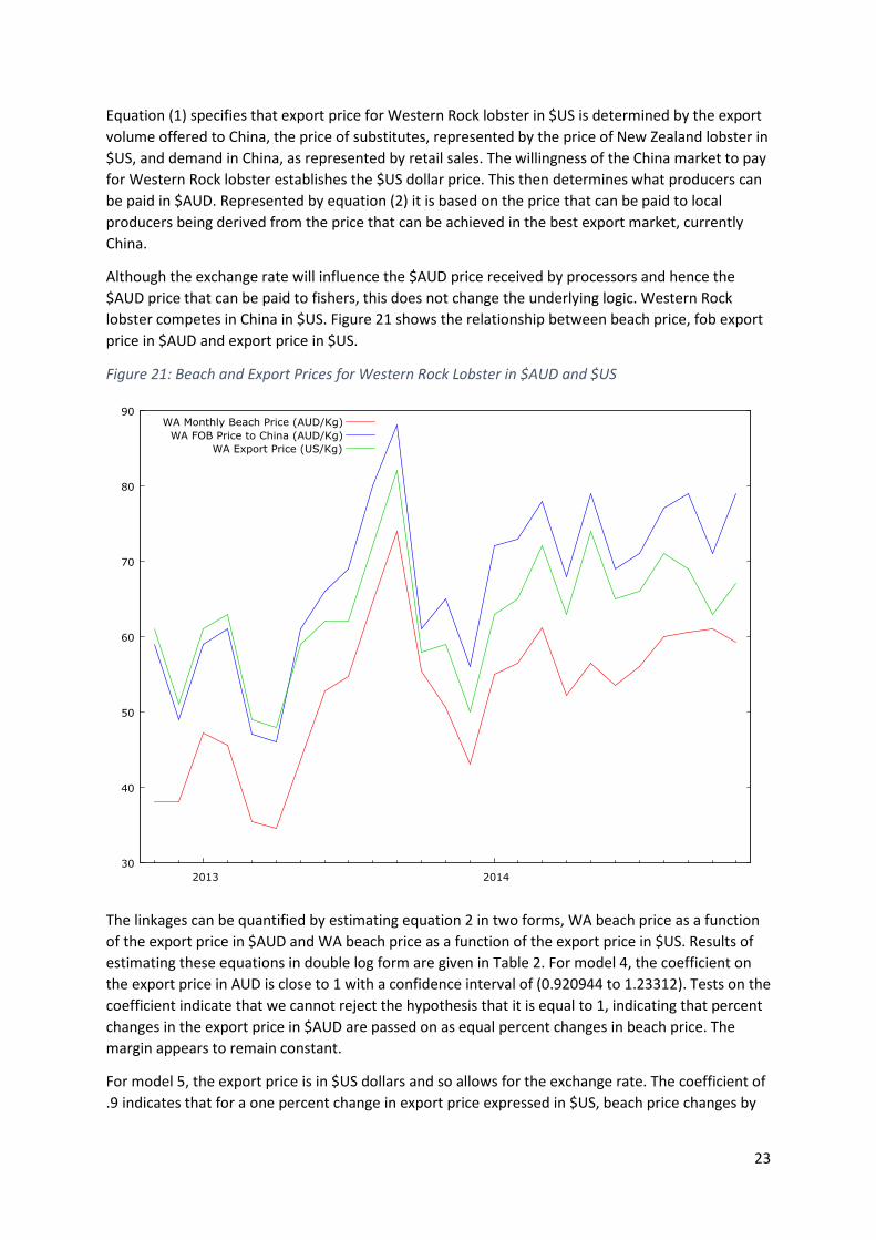
Although the exchange rate will influence the $AUD price received by processors and hence the
$AUD price that can be paid to fishers, this does not change the underlying logic. Western Rock
lobster competes in China in $US. Figure 21 shows the relationship between beach price, fob export
price in $AUD and export price in $US.
Figure 21: Beach and Export Prices for Western Rock Lobster in $AUD and $US
The linkages can be quantified by estimating equation 2 in two forms, WA beach price as a function
of the export price in $AUD and WA beach price as a function of the export price in $US. Results of
estimating these equations in double log form are given in Table 2. For model 4, the coefficient on
the export price in AUD is close to 1 with a confidence interval of (0.920944 to 1.23312). Tests on the
coefficient indicate that we cannot reject the hypothesis that it is equal to 1, indicating that percent
changes in the export price in $AUD are passed on as equal percent changes in beach price. The
margin appears to remain constant.
For model 5, the export price is in $US dollars and so allows for the exchange rate. The coefficient of
.9 indicates that for a one percent change in export price expressed in $US, beach price changes by
30
40
50
60
70
80
90
2013 2014
WA Monthly Beach Price (AUD/Kg)
WA FOB Price to China (AUD/Kg)
WA Export Price (US/Kg)

24
.9 of a percent. However, the confidence interval is (0.678839 to1.13892) and we cannot reject the
proposition that its true value is also equal to 1.
Table 2 Estimates of beach price – export price relationship
Using observations 2012:11-2014:11 (T = 25)
Dep variable Log Beach Price Log Beach Price
Model 4 $AUD Model 5 $US
Coefficient t-ratio t-ratio
Const −0.578309
(0.31684)
-1.83 0.166152
(0.462273)
0.3594
Log WA_x_price ($AUD) 1.07703
(0.07545)
14.27 ***
Log WA_x_price ($US) 0.908879
(0.111203)
8.1732 ***
Statistics based on the rho-differenced data:
rho = -.00513 0.705718
Mean dependent var 3.9407 3.9407
S.D. dependent var 0.1949 0.1949
R-squared 0.8978 0.8830
Adjusted R-squared 0.8934 0.87798
F(3, 45) 206.875 444.231
P-value(F) 5.5e-13 1.54e-16
Durbin-Watson 1.65 1.56
Combined Model
An equilibrium relationship to explain beach prices could effectively combine equations (1) and (2)
for an export dominated market. This would make beach price a function of catch and the drivers
contained in equation (1). Various specifications for this model can be considered. These are
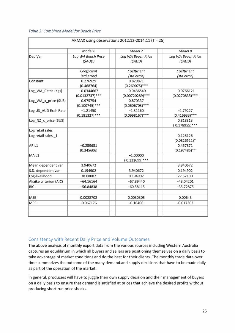
reported in Table 3. Models 6 and 7 explain beach price in term of catch volume, export price in $US
and the US/AUD exchange rate. Model 6 has an AR specification, AR(1,0,0) and Model 7 has an MA
specification, MA(0,0,1). Model 7 appears to be marginally better based on the information criteria.
However, there is little to choose between them. Both confirm the relatively small impact of
monthly changes in catch on local beach price when the export price and exchange rate are held
constant.
Model 8 replaces the $US export price with the independent variables that were determined to have
a major influence on this export price and reported in Table 1. Here the beach price is explained
using the catch volume, the price of NZ lobster in $US, retail sales in China lagged one period and the
exchange rate. As a model to explain beach price on a monthly basis Model 8 appears to be less well
performed based on the information criteria. It does produce results consistent with the previous
ones in terms of the impact of catch volume and the impact of retail sales on price with, for
example, an impact of 0.13% on price for a 1% increase in retail sales.
25
Table 3: Combined Model for Beach Price
ARMAX using observations 2012:12-2014:11 (T = 25)
Model 6 Model 7 Model 8
Dep Var Log WA Beach Price
($AUD)
Log WA Beach Price
($AUD)
Log WA Beach Price
($AUD)
Coefficient
(std error)
Coefficient
(std error)
Coefficient
(std error)
Constant 0.276929
(0.468764)
0.829871
(0.269075)***
Log_WA_Catch (Kgs) −0.0344667
(0.0132737)***
−0.0436540
(0.00720289)***
−0.0766121
(0.0270835)***
Log_WA_x_price ($US) 0.975754
(0.100745)***
0.870337
(0.0606703)***
Log US_AUD Exch Rate −1.21450
(0.181327)***
−1.31160
(0.0998167)***
−1.79227
(0.416933)***
Log_NZ_x_price ($US) 0.818813
( 0.178955)***
Log retail sales
Log retail sales _1 0.126126
(0.0826511)*
AR L1 −0.259651
(0.345606)
0.457871
(0.197485)**
MA L1 −1.00000
( 0.131699)***
Mean dependent var 3.940672 3.940672
S.D. dependent var 0.194902 3.940672 0.194902
Log-likelihood 38.08082 0.194902 27.52100
Akaike criterion (AIC) −64.16164 −67.89440 −43.04201
BIC −56.84838 −60.58115 −35.72875
MSE 0.0028702 0.0030305 0.00643
MPE -0.067176 -0.16406 -0.017363
Consistency with Recent Daily Price and Volume Outcomes
The above analysis of monthly export data from the various sources including Western Australia
captures an equilibrium in which all buyers and sellers are positioning themselves on a daily basis to
take advantage of market conditions and do the best for their clients. The monthly trade data over
time summarizes the outcome of the many demand and supply decisions that have to be made daily
as part of the operation of the market.
In general, producers will have to juggle their own supply decision and their management of buyers
on a daily basis to ensure that demand is satisfied at prices that achieve the desired profits without
producing short run price shocks.
26
The equilibrium trade data suggest that over the recent past, the outcomes of these myriad and
complex daily supply, buying and pricing decisions has been to produce a balance between demand
and supply growth that, as documented in the above analysis, has expanded revenues. In this sense,
they indicate that over the recent past, the summary outcome is that demand growth has allowed
suppliers, including WA, to position greater export volumes in Greater China without damaging
revenues, or, in most cases, prices.
While the monthly export data can be interpreted as establishing equilibrium prices for the various
volumes that producers have chosen to offer, intra-month data, such as daily price and volume
adjustments reflect more the underlying micro decisions that producers, in particular processors,
have to make to ensure that over time they achieve an orderly and successful market outcome.
Using the monthly data, we assume that demand and supply is reconciled within a month. For daily
data, the end of day position may be that buyers are unsatisfied or that supply must be put into
inventory. Hence, daily data on beach price and volumes would not normally be used to estimate
simple inverse demand equation of the kind documented in equation (1).
However, as documented by the Department of Fisheries, the 2013 and 2014 years appear to have
been characterized by situations where toward the end of the year, the remaining TACC shrunk and
daily prices rose as a way of rationing off demand from buyers. This is consistent with the above
analysis. Within any given month, we expect decisions to be made that reconcile buyers and sellers.
Processors are key to this. If TACC is near depleted toward year-end, we expect daily prices to rise to
ration demand and produce the required reconciliation.
Nevertheless, it is instructive to consider the consistency of the above analysis with the outcome
from 2013 and 2014 and the implications of the results for possible future intra-year pricing
patterns.
As noted above, if demand drivers continue to shift demand to the right the potential exists for
export prices to continue to rise.
Let Dg be expected demand growth and Sg be expected supply growth.
If Dg> Sg then there is upward pressure on prices. As documented above, this scenario is the one
that best explains the recent trend in export prices to China.
From a WA perspective, in recent years Sg is approximately zero because the TACC has not changed.
This is also effectively true for supply to Greater China as all supply is now sold as exports to China.
If we extrapolate the continued growth in demand then from a Western Australian perspective, it is
plausible that for immediate future years, Dg>Sg because with a constant TACC, Sg=0. This scenario
is, ceteris paribus, likely to put upward pressure on export prices in China. How this affects the intra-
year pattern depends on the managements of daily deliveries from fishers and daily demands from
buyers. Although processors can influence daily deliveries through price signals, it appears that this
is less than perfect. If Dg>Sg, the upward price pressure is likely to be evident throughout the year.
Compared to the previous year fishers are likely to experience higher prices from the start. Banking
higher prices early in the year may encourage early catch potentially resulting in a tendency to have
limited quota left toward the end of the year. Hence, the experience of 2013 and 2014 is perfectly
consistent with a case where demand is high relative to supply and where there is less than perfect
ability to spread catch patterns over the year.
27
Summary and Conclusion
Findings
In this report, the trends and drivers in the lobster export market have been analysed. Since the
move to ITQ, we have 49 months of detailed export data to assess.
Over that period, several notable trends have emerged in export volumes. Most notably:
• Greater China has become a focus for all exporters from Australia and New Zealand and
more recently from other jurisdictions, such as the US.
• Western Australian exports to Greater China have grown to the point where virtually all
exports are to Greater China. This has occurred against the backdrop of a reduction in total
catch and reflects a distinct switch to China from other markets over the period.
• Since 2008, in part, it appears because of the fall in demand in Europe; the US has ramped
up its export volumes to Greater China markedly.
The data suggest that, even though export volumes have grown, prices have not been significantly
affected. In $US, export prices for Western and Southern Rock lobster have trended up over the
period. Perhaps even more significantly, the massive volume increases into China from the US have
had only a marginal impact on their export price. It has in fact been relatively constant over the
period.
One important consequence of these trends is that revenues received have also grown. This is true
for exporters experiencing volume and price increases. Western Australia fits into this category.
More significantly, it is also true for the US where, despite the large volume increases, the
consequential modest price fall has meant that aggregate export revenue increased. The US export
price reduction over the period has been more than offset by the volume increase.
It appears that over the period, growth in demand in China has been able to absorb the increase in
volumes from these major suppliers without damaging prices and revenues. In effect, demand in
China has been growing and outstripping the growth in supply.
This result is confirmed by the estimation of the inverse demand curve (equation 1) for Western
Australian export price using the monthly data. The retail sales variable is a positive influence on
price is a statistically significant variable. Along with the price of substitutes (such as New Zealand
Southern Rock lobster price), it is more significant than the export volume for Western Australian
Rock lobster. Monthly volume fluctuations affect price, but are less significant than the price of
substitutes and demand drivers in China. The equation implies a high price elasticity of demand,
consistent with the constant price assumption used by Gordon for modelling of the Canadian lobster
export supply chain (Gordon 2011). Modelling beach price indicates that beach price bears a stable
relationship to export price measured in AUD and to export prices measured in USD. For both cases,
we cannot reject the hypothesis that the estimated coefficient is 1 meaning that a 1% gain in export
price increases beach price by 1%.
The beach price might also be explained by a combined model where, in addition to catch, either the
export price of the variables determining the beach price are included as explanatory variables.
Estimates for these model specifications reinforced findings from the estimation of the inverse
demand curve and beach price curve. Export price, and exchange rate are major drivers of beach
price and need to be considered in conjunction with catch fluctuations to explain beach price. The
same applies to models where more fundamental drivers are included as explanations of beach price
28
in place of export price. The price of substitutes and retail sales are both important in explaining
beach price alongside catch volume.
Notwithstanding the consistency of the results across different levels of analysis and different model
specifications, it is important to note that the time series is relatively short since the system of ITQs
was established. Pricing and marketing will continue to evolve and ultimately a longer monthly time
series incorporating variations in TACC is required to fully test these various demand propositions
and develop forecasting models. This is a consideration when translating results to the future.
Looking Forward
The results suggest that, if the recent past since the WA ITQ was implemented, can be extrapolated
forward, demand from China will continue to grow and there will be upward pressure on prices, or
at least no significant downward pressure.
If this was the case, then an increase in export volumes from Western Australia, New Zealand or
other sources in future could be expected to have little impact on prices, so long as the increase was
in balance with projected demand growth over the comparable period.
This begs several key questions, namely:
• Will Chinese demand for lobster continue to expand and be the major driver shifting
demand to the right at the current rate, or an even higher rate?
• What will be the supply response from competitive jurisdictions? Will this grow as per the
US in recent past, stabilize or even decline? For a given expected demand growth, all other
things equal, the last scenario implies price rises, while stabilization of supply growth implies
more modest price rises. Only a significant supply response could impose a price fall, and
only then if it outstripped demand growth.
While the past is relevant, there is a case that specific analysis is needed of future demand
drivers, likely supply responses and possible price impacts. In particular, when exports to
mainland China switch from the indirect to direct channels under the FTA arrangements, will this
open up other internal city markets for lobster, growing demand even more? Will European
demand resuscitate causing some US supply to divert back?
Past data does not inform these predictions. However, based on the analysis of export data to date,
it does suggest that for best guess supply and demand responses, a modest increase in supply by any
one exporter is unlikely to stop the general upward price trend.
Whilst demand analysis is valuable in that it directs us to likely price increases, on its own, it cannot,
determine the profit maximizing level of exports. Exports are harvested from a managed biomass.
Targets relating to biomass, actual expected biomass and CPUE and even the objectives, other than
simple profit of fishers, need to be taken into account, as does the risk attitude of managers and
fishers to harvesting the biomass and pursuing profit.
Finally, it is worth noting that the trade data captures an equilibrium in which all buyers and sellers
are positioning themselves on a daily basis to take advantage of market conditions and do the best
for their clients. The monthly trade data over time summarizes the outcome of the many demand
and supply decisions. In this sense, they indicate that over the recent past, the summary outcome is
that demand growth has allowed suppliers, including Western Australia, to position greater export
volumes in Greater China without damaging revenues, or in most cases prices. Of course, if any
supply response occurred in too short a period, say intra month; it could produce substantial short
29
term price fluctuations that the market would have to manage. The data suggest that over the
recent past, any such outcomes have been managed to produce a balance between demand and
supply growth that, as documented in the above analysis, has expanded revenues.
References
Gordon, Daniel V. 2011. Canada_Price_realtionships_fish_supply_chain. Rome. Retrieved
(http://www.fao.org/search/en/?cx=018170620143701104933%3Aqq82jsfba7w&q=price+relat
ionships+in+canadian&cof=FORID%3A9&siteurl=www.fao.org%2Fhome%2Fen%2F&ref=www.g
oogle.com%2Furl%3Fsa%3Dt%26rct%3Dj%26q%3D%26esrc%3Ds%26source%3Dweb%26cd%3
D1%26ved%3D0CB4QFjAA%26url%3Dhttp%253A%252F%252Fwww.fao.org%252F%26ei%3DkP
BjVYGLG9fr8AX4rYHYCQ%26usg%3DAFQjCNFN0FJRtsVrfnxh2u66Un8onLMaSw%26bvm%3Dbv.
93990622%2Cd.dGc&ss=13607j17673193j39).
Norman-López, Ana et al. 2014. “Price Integration in the Australian Rock Lobster Industry:
Implications for Management and Climate Change Adaptation.” Australian Journal of
Agricultural and Resource Economics 58(1):43–59.
Data Sources.
Australian Bureau of Statistics (2014). International Trade Customised Report. Canberra: ABS.
China National Bureau of Statistics (2015). Retail Sales Monthly. Data extracted in real time from:
http://data.stats.gov.cn/english/easyquery.htm?
Statistics NZ (2014). Harmonized Trade Exports. Wellington.NZ Statistics. Data extracted in real time
from: http://www.stats.govt.nz/infoshare/TradeVariables.aspx?DataType=TEX.
United Nations Trade Statistics Division (2015) UN Commtrade Data Base. available from :
http://comtrade.un.org/data/
United States Census (2015). USA Trade Online. Data extracted in real time from
https://usatrade.census.gov