An Analysis of Ozone Monitoring Seasons in the U.S. Louise Camalier (not attending) (Presented by David Mintz) National Air Quality Conference Portland,

An Analysis of Ozone Monitoring Seasons in the U.S.

Louise Camalier (not attending)

(Presented by David Mintz)National Air Quality Conference

Portland, Oregon April 8, 2008

Purpose

The ozone NAAQS level is now 0.075 ppm

Are states’ current official monitoring seasons adequate to protect against the adverse health effects protected by the

future primary air quality standard?

Analytical Plan

Use most recently certified 3-yr period 2004-2006

Look at ambient data, examine actual exceedences

Predict ozone to examine potential exceedences (across time) Useful for monitors without year round

data

Official Monitoring SeasonsCurrent CFR vs. AQS Current CFR (mandated season)

Generally, seasons are consistent within a state, excluding Texas and Louisiana (defined by AQCR)

AQS (mandated & modified season) Seasons can be modified on a site-by-site basis,

based on judgment of regional administrator Examples:

California, Nevada, Arizona

May-Sep

Mar-OctMar-Sep

Mar-Nov

Jun-Sep

Apr-Nov

MonitoringSeason

Apr-Oct

Official Ozone Monitoring SeasonsWhere is the year round monitoring?

Good spatial representation

Year round monitoring

Official seasons in AQSMonitoring Data in AQS

Jan-Dec

Apr-SepMay-Oct

Wisconsin is April 15 -

Sept 15

Using Ambient Data What do we see?Ambient, year round data from 531 sites (~45% of total)

Examine number of observed exceedances (8hr daily max) using as much data as possible

Full year Partial year Only within monitoring season

With the data available, are we seeing exceedances occurring outside of a state’s official season?

Exceedances: in or out of season? Common (“core”) monitoring season across all states is

June-Sept Months displayed on the following maps are the “fringe”

months Feb-May (4 months before) Nov-Jan (4 months after)

Are there out of season exceedances when the concentration threshold is lowered?

Scenarios: 0.075 ppm 0.060 ppm*

*indicator for the yellow “AQI” level

Ozone AQI Summary

Category AQI ValuePrevious 8-Hour

Ozone AQI(ppm)

New 8-HourOzone AQI

(ppm)

1-HourOzone AQI

(ppm)

Good 0-50 0.000-0.064 0.000-0.059

Moderate 51-100 0.065-0.084 0.060-0.075

Unhealthy of Sensitive Groups

101-150 0.085-0.104 0.076-0.095 0.125-0.164

Unhealthy 151-200 0.105-0.124 0.096-0.115 0.165-0.204

Very Unhealthy 201-300 0.125-0.374 0.116-0.374 0.205-0.404

Hazardous301-400 0.405-0.504

401-500 0.505-0.604

Changes are in red Used in conjunctionwith one another

Using the new standard (0.075 ppm) to locate areas that may need seasonal modifications

Standard scenario: 0.075 ppm

April

MarchFebruary

“in season” exceedances in blue“out of season” exceedances in red

May

4 months before common O3 season

2/1-2/27 3/30-3/31

This situation doesn’t in itself justify expanding the season for the entire month of March

October November

December

Standard scenario: 0.075 ppm“in season” exceedances in blue“out of season” exceedances in red

January

4 months after common O3 season

1/24-1/31

Using the AQI yellow level (0.060 ppm) to locate areas that may need seasonal modifications

February March

Scenario: 0.060 ppm

April May

“in season” exceedances in blue“out of season” exceedances in red 4 months before common O3 season

Scenario: 0.060 ppm

October November

December January

“in season” exceedances in blue“out of season” exceedances in red 4 months after common O3 season

Estimating ozone at existing sites when data is not available

Predicting during the off-season months

20 40 60 80

2060

100

Modeled Days

Predicted

Obs

erve

d

0 20 40 60 80

020

6010

0

All days with observations

PredictedO

bser

ved

0 5 10 15 20

05

1015

20

Number Exceedance Days(Months with any Observed data)

Predicted

Obs

erve

d

Jan

Feb

Mar

Apr

May

Jun

Jul

Aug

Sep Oct

Nov

Dec

Predicted exceedances days above 60

05

1015

Columbia, SC OzoneTarget months in red(Fit months = 3, 4, 5, 9, 10 )

Why Statistically predict ozone? We would like to “fill”

temporal gaps where little or no ozone data are available

Statistical model is used and tailored to accurately predict exceedance rates during off-season months*

Off season month ranges are area specific but typically include months such as February, March, October and November

*Assumes that relationship between ozone and meteorology during other months is similar to data used in fitting (do not use core months)

Example for South Carolina

Red dots are data in the predicted months

Statistical Prediction of Ozone(in non-monitored months)

Case Study: Columbia, South Carolina

South Carolina’s official monitoring season: April - September We want to predict ozone during months outside of the official

season Focusing on predicting for: February, March, and October Core months for ozone season: June, July, and August Ozone and meteorological relationships are different during

“core” months, therefore we only use the surrounding (cooler) months (March, April, May, September, and October) in the model

Using the cooler months is best as this better represents the kind of meteorology and ozone response that occurs during the months which we are trying to predict

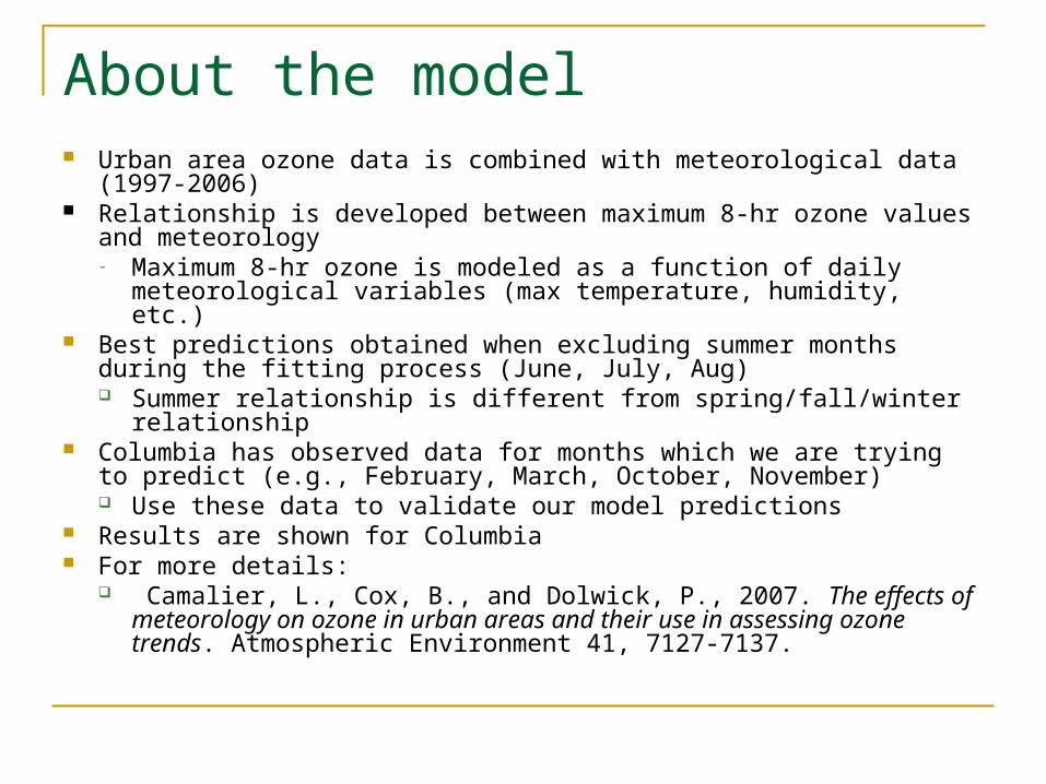
About the model Urban area ozone data is combined with meteorological data (1997-

2006) Relationship is developed between maximum 8-hr ozone values and

meteorology- Maximum 8-hr ozone is modeled as a function of daily

meteorological variables (max temperature, humidity, etc.) Best predictions obtained when excluding summer months during the

fitting process (June, July, Aug) Summer relationship is different from spring/fall/winter relationship

Columbia has observed data for months which we are trying to predict (e.g., February, March, October, November) Use these data to validate our model predictions

Results are shown for Columbia For more details:

Camalier, L., Cox, B., and Dolwick, P., 2007. The effects of meteorology on ozone in urban areas and their use in assessing ozone trends. Atmospheric Environment 41, 7127-7137.

Example: Columbia, South Carolina

Scatter plot of observed and predicted values for only the data used in the fitting process (March, April, May, Sept, Oct)

Scatter plot of observed and predicted number of exceedances for all month/year combinations (2004-2006) with observed data

Values in red not used in fitting process (February, November)

Model Validation

20 40 60 80

2060

100

Modeled Days

Predicted

Obs

erve

d

0 20 40 60 80

020

6010

0


Predicted

Obs

erve

d

0 5 10 15 20

05

1015

20


PredictedO

bser

ved

Jan

Feb

Mar

Apr

May

Jun

Jul

Aug

Sep Oct

Nov

Dec


05

1015


20 40 60 80

20

60

100

Modeled Days

Predicted

Observ

ed

0 20 40 60 80

020

60

100


Predicted

Observ

ed

0 2 4 6 8

02

46

812


Predicted

Observ

ed

Jan

Feb

Mar

Apr

May

Jun

Jul

Aug

Sep

Oct

Nov

Dec


01

23

4


exceedances > 75 ppb occur in months outside of current monitoring season (red bars)

Jan 0Feb 0Mar 0.6April 3.4May 4.8June 3.9July 3.7Aug 1.2Sep 0.7Oct 0.1Nov 0Dec 0

Columbia, South Carolina

June, July, and August are not used in the fitting process, however they are behaving the way we expect

Using ambient & predicted dataCase Example: South CarolinaSeason: April-September Used urban area with highest

expected exceedences

Ambient Data (2004-2006) On average, for 60 ppb

~10 exceedences/year between 2/15-3/31

We are predicting ~8 exceedences/year between February and March

20 40 60 80

2060

100

Modeled Days

Predicted

Obs

erve

d

0 20 40 60 80

020

6010

0


Predicted

Obs

erve

d0 5 10 15 20

05

1015

20Number Exceedance Days

(Months with any Observed data)

Predicted

Obs

erve

d

Jan

Feb

Mar

Apr

May Jun

Jul

Aug

Sep Oct

Nov

Dec


05

1015


Feb: 1.2March: 6.4

Predicted Exceedences, days above 60 ppb

predicted months

Conclusions

One can use ambient, existing data along with statistically predicted data to guide informed decisions

Any modifications of the official season will be based on monitoring judgment and the results from this analysis

Other Questions?

Contact: Louise Camalier

[email protected]

(919) 541-0200

EPA,OAR,OAQPS,AQAD, Air Quality Analysis Group (RTP, NC)

Documents

An Analysis of Ozone Monitoring Seasons in the U.S. Louise Camalier (not attending) (Presented by David Mintz) National Air Quality Conference Portland,