Embed Size (px)
Citation preview

An analysis of bidding strategies in the Danish wind power market En analyse av strategisk budgivning i det danske vindkraftmarkedet
Norwegian University of Life Sciences Faculty of Social Sciences School of Economics and Busines
Master Thesis 2014 30 credits
Nabeela Qureshi
brought to you by COREView metadata, citation and similar papers at core.ac.uk
provided by NORA - Norwegian Open Research Archives

I want to dedicate this work to my mother.
She has been my strength and my biggest encouragement.
I

II

Preface
This Master thesis is a final project towards my Master's degree in Business and
Administration at the Norwegian University of Life Sciences. The topic of this thesis is
selected in accordance to my major programme, Energy economics.
I want to sincerely thank my supervisor Olvar Bergland for his guidance. His advice and
support has been very helpful to me, and he has been available for me during the whole
process and considered all my questions.
I want to mention my family and my fiancé Farid Esam and thank them for their
continuous support. I also want to thank my friend at the university, Senyonga
Livingstone for all the meaningful discussions during the process.
Ås, 15th May 2014
Nabeela Qureshi
III

IV

Summary
In 2013 the wind turbines in Denmark accounted for approximately 30 % of Denmark's
total electricity supply (Jensen and Sørensen 2014). The 2020 goal necessitates wind
supply increase from 30% to 50 % (Lentz and Strandmark 2014). The expansion of the
wind power sector raises several questions regarding its strategic effect on the spot and
the regulation market. The suspicion is that increased amount of wind power will trigger
systematic use of the regulation market. The area of focus is West-Denmark and the
problem for discussion is stated in this manner: How does deviation between predicted
production and actual production of wind-power in West-Denmark affect the bidding in
the spot market?
The interest is to use the regulation market and wind prognosis to find the deviations
between the supply bids made to the spot market, and actual delivery. The bids made to
Nord Pool are confidential. The analysis is done without this information. Two
hypotheses are formulated in order to answer the problem of discussion, and two models
are developed in order to test these hypotheses Model 1 and Model 2.
In Model 1 the effects of up and down regulation are tested on price for balancing
regulation. The goal in this model is to reveal the relationship between up and down-
regulation price to check for asymmetries in the regulation market. In Model 2 wind
power production is tested, as an exogenous predictor of total regulation. The data used to
test Model 1 and Model 2 is downloaded from energinet.dk, except the data on wind
prognosis. The data on wind prognosis is downloaded from Nord Pool´s website. The
data downloaded is from 01.01.2012 to 31.12.2013. The estimation strategy in Model 1 is
the use of OLS, and the estimation strategy in Model 2 is based on regression analysis
with possible measurement error, where wind prognosis is used as an instrumental
variable. The findings in Model 1 suggest that there is difference in price for up-and
down regulation, and that the use of the regulation market is slightly asymmetric.
The findings in Model 2 rejected the second hypothesis, and wind power production is an
endogenous predictor of total regulation. The deviation between planned and actual
production of wind power can be used as an incentive to place the supply bids
strategically on the spot market, to obtain a better price in the regulation market.
V

Significant measurement error in Model 2 can be regarded as indirect evidence of
systematic action.
VI

Sammendrag
I 2013 stod vindkraftsektoren for 30 % av den totale kraftproduksjonen i Danmark, (
Jensen og Sørensen 2014 ). Et mål for år 2020 er en økning fra 30% til 50% ( Lentz og
Strandmark 2014 ). Den planlagte utvidelsen av vindkraftsektoren reiser flere spørsmål
rund strategisk budgivningsadferd i spot og kraftreguleringsmarkedet. Det mistenkes at
ved økt vindkraft i kraftsystemet vil det utløse systematisk bruk kraftreguleringsmarkedet.
Denne analysen begrenser seg til Vest-Danmark og problemstillingen er formulert som
følgende: Hvordan vil et avvik mellom planlagt og faktisk produksjon av vindkraft i Vest-
Danmark påvirke budgivning i spotmarkedet?
Hovedmålet er å bruke reguleringskraftmarkedet og vindprognose for å finne avvik
mellom bud i spot markedet og faktisk levert produksjon. Budgivningen i Nord Pool
regnes som konfidensiell og problemstillingen besvares uten denne informasjonen. For å
besvare problemstillingen er det i hovedsak formulert to hypoteser, og hypotesene ble
testet basert på to modeller, modell 1 og modell 2.
I modell 1 blir effekten av opp -og nedregulering testet mot prisen i
kraftreguleringsmarkedet. Målet er å klargjøre forholdet mellom opp –og
nedreguleringsprisen for å gjennomskue potensielle asymmetrier i
kraftreguleringsmarkedet. I modell 2 blir vindkraftproduksjon testet som en eksogen
variabel til å predikere den totale reguleringen i kraftreguleringsmarkedet. Begge
modellene er basert på data som er hentet fra energinet.dk, bortsett fra data for
vindprognose, som er hetet fra hjemmesiden til Nord Pool. Dataen gjelder fra 01.01.2012
til 31.12.2013. OLS metoden ble brukt til å estimere modell 1. Estimerings strategien til
modell 2 faller under 2SLS der vindprognosen ble brukt som en instrumentell variabel.
Modell 2 ble testet for systematiske målefeil.
Hovedfunnene i modell 1 indikerer en prisforskjell mellom opp -og nedregulering. I
tillegg er det hint av asymmetrier når det kommer til bruken av kraftreguleringsmarkedet.
Funnene i modell 2 indikerer at vindkraftproduksjon er en endogen variabel i
sammenheng med total regulering. Avviket mellom planlagt og virkelig produksjon av
vindkraft kan brukes som et insentiv systematisk vis anlegge bud på spotmarkedet.
Betydelig målefeil i Modell 2 kan anses som indirekte bevis på systematisk handling for å
få en bedre pris i reguleringskraftmarkedet.
VII

VIII
Table of contents 1 Introduction .................................................................................................................................... 1
1.1 Background ............................................................................................................................ 1
1.2 Problem for discussion ........................................................................................................... 2
1.3 Structure ................................................................................................................................. 3
2 Nord Pool and strategic behaviour ................................................................................................. 5
2.1 The Nordic electricity exchange ............................................................................................. 5
2.1.1 Elspot .............................................................................................................................. 6
2.1.2 Imbalance in the power market ...................................................................................... 6
2.1.3 Regulation market .......................................................................................................... 7
2.1.4 Implicit auctions and trade ............................................................................................. 8
2.1.5 Electricity contracts in the financial market ................................................................... 8
2.2 Wind power and Danish bidding areas ................................................................................... 9
2.2.1 Future investments ........................................................................................................ 10
2.3 Bidding and strategies .......................................................................................................... 10
2.3.1 Market power................................................................................................................ 10
2.3.2 The regulating power market on the Nordic power exchange ...................................... 11
2.4 Summary .............................................................................................................................. 13
3 Theory and Model ........................................................................................................................ 15
3.1 Balance equation .................................................................................................................. 15
3.1.1 Model 1 ......................................................................................................................... 16
3.1.1.1 Modification of Model 1 .......................................................................................... 18
3.1.2 Model 2 ......................................................................................................................... 19
3.1.3 Hypotheses and model summary .................................................................................. 22
4 Data .............................................................................................................................................. 25
4.1 The variables ........................................................................................................................ 25
4.2 Descriptive statistics ............................................................................................................. 26
5 Estimation and analysis ................................................................................................................ 29
6 Results and discussion .................................................................................................................. 31
6.1 Results Model 1 .................................................................................................................... 31
6.1.1 The average price of up-regulation and down-regulation ............................................. 33
6.2 Results Model 2 .................................................................................................................... 34
6.2.1 Total regulation ............................................................................................................ 34
6.2.2 Estimated parameters Model 2 ..................................................................................... 36
IX
6.2.3 OLS estimation with wind power production .............................................................. 37
6.2.4 Wind prognosis as a proxy variable ............................................................................. 37
6.2.5 The instrumental variable approach ............................................................................. 38
6.2.6 Measurement error ....................................................................................................... 39
6.3 Discussion of results ............................................................................................................ 39
7 Conclusions .................................................................................................................................. 45
References ............................................................................................................................................ 46
Appendix 1 ............................................................................................................................................. A
Appendix 2 ............................................................................................................................................. C
Appendix 3 ............................................................................................................................................. E
X

List of Figures Figure 1: Wind power capacity and wind-power’s share of domestic supply (Jensen & Sørensen 20014). .......... 9 Figure 2: Price of regulating power (Skytte 1999). .............................................................................................. 17 Figure 3: Daily up and down regulation. .............................................................................................................. 34 Figure 4: Distribution of the variable total regulation. ......................................................................................... 35
List of Figures Table 1: Descriptive statistics of the variables. .................................................................................................... 27 Table 2: Estimated parameters model 1. ............................................................................................................... 31 Table 3: Estimated parameters OLS, OLS_Proxy, 2SLS ..................................................................................... 36
XI

XII
1 Introduction
An analysis of bidding strategies in the Danish power market “This asymmetric cost may encourage bidders with fluctuating production to be more
strategic in their way of bidding on the spot market. By using such strategies the extra costs for e.g. wind power needed to counter unpredictable fluctuations may be limited”
(Skytte 1999)
How does deviation between predicted production and actual production of wind-power in West-Denmark affect the bidding in the spot market?
1.1 Background
This thesis is inspired by the quote presented above, taken from Klaus Skytte's article “The
regulating power market on the Nordic power exchange, Nord Pool” published in 1999. His
research and findings suggest that the cost of using the regulation power market is dependent
on the spot price level at the Nordic power exchange. He discovered that the regulation cost
was more correlated to the spot price in an event of down-regulation, compared an event of
up-regulation. With expected fluctuation of supply and demand, the actor in the market is
able to jointly optimize his total bids at the spot market and in the regulation market (Skytte
1999). His research targeted Norwegian hydropower producers.
Skytte's article was written before Denmark joined the Nordic power exchange, Nord Pool, in
year 2000 (NordPool 2013). Today Denmark's wind power production covers 30 % of the
country´s energy production. An analysis of the current effects of the wind power supply bids
submitted in Nord Pool may provide insights that can determine the hidden cost or as Skytte
described, strategic bidding behaviour related to fluctuating power supply. Within year 2020
wind energy production is planned to increase, and will account for 50 % of the total energy
production in Denmark (Danish Wind Industry Association 2014). According to these plans
the amount of wind power in the system will increase. A research on wind power production
in West-Denmark and up- regulation was published in 2007, the article concluded the
1

relation as significant (Forbes et al. 2007). By using updated data from 2012-2013 and
modified version of the model discussed in Skytte's article the goal of this thesis is to detect
any indication of strategic behaviour in the Danish wind power market, by analysing the
bidding strategies related to wind power supply. The bidding area of interest is West-
Denmark, and their use of regulation services.
It seems like that the suspicion of strategic behaviour lies in the bidding behaviour of the
wind power producers. The suspicion is that they systematically bid less wind power supply
than the predicted amount, and then use the regulation market to down regulate the excess
supply. If asymmetries are found in the regulation market, further analysis of this thesis will
test the regression model for systematic measurement error. Whether systematic behaviour is
an economic burden or has any spillover effects on other actors in the market will depend on
the magnitude of the problem, and is not discussed in this thesis. This thesis will focus on
indirect evidence of strategic behaviour in the bidding area of West-Denmark.
1.2 Problem for discussion
How does deviation between predicted production and actual production of wind-power in West-Denmark affect the bidding in the spot market?
The interest here is to use the regulation market and the wind prognosis to find the deviations
between supply bids made at the spot market, and actual delivery. There is no official data on
the bids submitted into Nord Pool, as the data is confidential. Therefore problem stated will
be answered without using this data, and the problem for discussion will be answered based
on these hypotheses:
Hypothesis one: There is no systematic relationship between regulation price, and up or
down- regulation.
The alternative hypothesis is that there is a systematic relationship between regulation price
and up or down-regulation.
Hypothesis two: Wind power production is an exogenous predictor of total regulation
2

The alternative hypothesis will reject hypothesis two and state that wind power production is
endogenous and measured with error.
1.3 Structure
The first chapter of this thesis reveals the problem for discussion and the related hypotheses
to be tested. The second chapter provide an overview of Nord Pool, earlier research on
strategic behaviour in the power market, and the Danish bidding areas. In the third chapter,
the two models behind the analysis are introduced with the relevant indication of the theory
behind them. The data and variables used in the analysis of the models are given in chapter
four. In chapter five the estimation, strategy and the analysis structure are given. The results
are specified and discussed in chapter six before concluding remarks in the final chapter.
3

This page intentionally left blank.
4

2 Nord Pool and strategic behaviour
This chapter is divided into four sections. Firstly the conceptual framework behind the
Nordic electricity market is presented. Secondly the Danish power market, bidding areas and
their future investment plans is discussed in the second part. In the third part of this chapter,
the earlier research on strategic behaviour is discussed before a brief chapter summary is
provided.
2.1 The Nordic electricity exchange
Nord Pool is the Nordic electricity exchange with member countries Denmark, Norway
Sweden, Finland, Estonia, and Lithuania. Electricity Producers, retailers, traders, and large
end users meet in the Nord Pool spot exchange to trade electricity. The producers need to pay
a fee to the grid owner for each kWh they pour into the grid, and the consumers need to pay a
fee for each kWh they draw from the grid. This is known as the point tariff system. This
system is relevant for understanding the key balance between production and consumption in
the system every hour (Nord Pool 2014a).
Each hour somewhere in the system the producer has to produce a certain amount of
electricity to the grid, and that same amount has to be consumed by the retailer´s customers.
Electricity grids transport the power, and for each local grid, there is a local grid operator
who handles the local low voltage grid. The TSO owns and operates the high voltage grid for
the respective country. Because the TSO own and operates the grid, it is solely responsible
for the assurance of supply in the country they are operating. The Danish TSO is
Energinet.dk, and it is a state-owned grid-company for both gas and electricity (Nord Pool
2014a).
5

2.1.1 Elspot
Electrical power in Nord pool is traded in a day-ahead auction market, Elspot. At noon, the
day before all supply and demand bids are cleared and transported to the grid. Both producers
and consumers meet in this market. At Nord Pool Spot in Oslo all the bids are received
electronically from market actors. (Nord Pool 2014a).
On an hourly basis the market price is given as the intersection between the aggregated
supply and demand curves. Price calculation is done and published by Nord Pool Spot. This
price is regarded as the system price, a theoretical price without any bottlenecks in the
system. The published information is then used by the TSO in the Nord Pool Spot area to
calculate the balancing power for producers and consumers. Both buyers and sellers have to
pay a trading fee to the market (Nord Pool 2014a).
In a competitive market a producer´s profit maximising outcome when price is equal to
marginal cost. Wind power producers have a marginal cost very close to zero if costs of
maintenance are not considered. Wind power is produced when the market price is positive
because the producers produce the amount above or equal to marginal cost of production. In
theory this is the structure of the supply bid for wind power producers. Marginal cost of
thermo-based power plants is not equal to zero and they have different marginal cost at
different capacities. This is how their bidding structure of production differentiates from
wind power producers (Nord Pool 2014b).
2.1.2 Imbalance in the power market
In the wholesale electricity market the process balancing the power at every hour depends on
all of the actors in the market. The TSO must ensure a balance between producers and
consumers. The storage possibilities with electricity are limited and in addition, it is
challenging to forecast the exact amount for production and consumption. A producer must
commit to the contract it has signed with the consumer. For example if a producer has a
contract of providing 100 MWh, and is only able to provide 90 MWh, the producer trades
6
with the TSO for the remaining 10 MWh, because the aim for the TSO is to always restore a
balance between the production and consumption (Nord Pool 2014a).
The imbalance in the power market is regulated by the TSO. Imbalance occurs when
consumption exceeds generation or generation exceeds consumption. To obtain a stable
frequency in the transmission grid, for instance if the stable frequency amount is 50 Hz, the
TSO has to make sure that the producers alter their production to obtain this level. When the
frequency in the system falls below 50 Hz, one or more producers will be asked to produce
more power to the grid, in other words TSO is regulating up the power supply. The TSO
regulate down when frequency exceed 50 Hz. To keep the frequency at 50 Hz, the TSO has
to trade the electricity in the market, and that electricity is called regulated power. The power
orders submitted into TSO under up or down regulation periods are ranked by increasing
price (Nord Pool 2014a).
2.1.3 Regulation market
Producers of fluctuating power make offers on the daily spot market in such way that they
can combine their production offers at the same price as generators of conventional power
sources. If the producers deviate from the commitment made to the daily spot market in that
exact moment for actual delivery, the producers will face an extra cost. The extra cost is
linked to the regulation expenses related to maintain the balance between demand and supply
in the spot market (Skytte 1999).
The regulating power market controls the entries that deviate from the power balance in the
market. This market closes two hours before the actual trade. When it is only 15 minutes
until market closure, the clearing is settled in the regulation market. When buyers increase
their purchases by buying of the excess supply, or when suppliers buy the excess supply to
increase their own supply, the actual payments of these transactions are made to the
regulating market. The payment is based on the balancing price for regulating power. The
spot market takes payment for all the commitments made to the spot market so therefore
limited attention is paid to the actual trade by the spot market (Skytte 1999). There is a fee
for using the regulation market called premium of readiness, and in addition, a fee is paid to
7
the spot market if the producer fails to keep the promises made to the spot market, i.e. the
bidding amount (Skytte 1999).
2.1.4 Implicit auctions and trade
When surplus and deficit of power occurs across the bidding areas, implicit auctions takes
place to obtain the welfare maximizing solution. There will be a price difference between the
surplus and deficit bidding areas. In theory, both areas are dependent on trade, and by trading
power the welfare-maximizing price will be obtained. Without trade, the area with surplus
will have a low price and the area with deficit will have a high price. Trade is only possible if
there is available transmission capacity in the transmission grid (Nord Pool 2014a).
Without transmission capacity, a price difference will occur due to the power imbalance.
When transmission capacity is available, implicit auctions are used to balance the price
differences. The price might not be the same, but with the electricity trade through the
implicit auction, the price difference will be reduced. If power trade was to happen cross-
border between two exchange areas due to bottlenecks in the system, both parties must give
their bid to a central organ to calculate the price. This is known as market coupling and this
happens between the Nordic, Central Western European and German exchange areas (Nord
Pool 2014a).
2.1.5 Electricity contracts in the financial market
There are several rules and regulations regarding trade of power in the exchange areas. The
players must be located in the same bidding area in order to trade electricity with each other.
Any trade across bidding areas is handled solely by Nord Pool Spot. Through the financial
electricity market, the players in different bidding areas have the opportunity to trade with
each other. The settlement is then regulated by a financial contract (Nord Pool 2014a).
A futures contract in the financial market regulates price and volume during the delivery
period. The average system price for the delivery period is compared to the hedge price of
8
the contract. If there is a deviation in price, that price difference times the volume is the
money amount transferred between the parties. In futures contracts the retailer compensates
the producer if the price is lower than the contract-regulated price, and the producer
compensates the retailer if the price is higher. Financial contracts regard only money and no
actual power is transferred between the parties (Nord Pool 2014a).
2.2 Wind power and Danish bidding areas
West Denmark (Jylland and Fyn) and East Denmark (Skjælland) are the two bidding areas
where the electrical system is divided in Denmark. West Denmark is interconnected with
East Denmark, Norway, Sweden and Germany (Energinett.DK 2014). The boundaries and
number of bidding areas are decided by the TSO. This trade that occurs between the bidding
areas, the orders must be submitted to Nord Pool Spot. (Nord Pool 2014a).
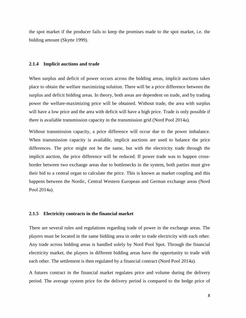
In 2013, the wind turbines in Denmark accounted for approximately 30 %, (94466/GWh) of
Denmark's total electricity supply (Jensen & Sørensen 2014). In December 2013 the installed
wind capacity was 4569 MW, and offshore wind power with a capacity of 517 MW. The
total number wind turbines in Denmark in December 2013 were 5176. The 2020 goal
necessitates wind supply increase from 30% to 50 % (Lentz & Strandmark 2014). Figure 1
gives an overview of the growth of renewable energy from year 1990 to 2012.
Figure 1: Wind power capacity and wind-power’s share of domestic supply (Jensen & Sørensen 20014).
9
2.2.1 Future investments
As earlier indicated, the Danish government has an ambition of expanding the renewable
energy to account for half of the country´s energy demand. There might be some obstacles
related to the plan. The necessary storage capacity needs to be developed to avoid negative
price periods and other complications. There are required technology related investments that
will be able to handle the intermittency and volatility when being dependent of renewable
resources (Kanter 2012). In addition, large investments are required to expand the offshore
wind –power compared to onshore energy sources. Improved weather forecasting is relevant
in order to anticipate the power production (Kanter 2012). Investments related to the
improvement could also affect the price due to increased cost.
2.3 Bidding and strategies
Detecting and classifying what is regarded strategic behaviour is not a straightforward task.
Every commodity market behaves differently, and each markets has its own rules and
regulation methods. Some findings from the Dutch and German market are given in this
section. The article by Klaus Skytte (Skytte 1999) is used to create the first model in the
analysis to detect any strategic- like behaviour. His findings will be highlighted in this
chapter, and his main analysis will create the base of Model 1 in chapter three.
2.3.1 Market power
Earlier research provides insight in strategic bidding models to identify gaming behaviour
(Dr. Petrov et al. 2003). This research paper focuses on the German and the Dutch power
market. When bidding at marginal cost, the bidding is regarded perfectly competitive. The
marginal cost in the competitive market is an aggregation of the marginal cost curves of all
participants in the market. The strategies were different in each market, and as a result, the
impacts of strategic behaviour were different. Taken the level of market share of the
company in consideration, two factors indicate to what extent strategic behaviour can be
10
profitable. First, it depends on how sensitive the market demand is to price, and second how
sensitive the firm is to a price change due to the supply of other companies in the market.
This can be narrowed down to two common strategies, capacity withdrawal and mark-up
pricing (Dr. Petrov et al. 2003).
In the Netherlands, the capacity from major power plants was withdrawn during peak
demand and price increased excessively. To be precise the price could be up to several
hundred Euros per MWh. Another significant finding in that market was that mark-ups only
increase with increased market demand. The sudden rise of mark-ups was linked to
substantial market power for some actors. The main result in the article was that there exists
a possibility of exercising market power both in the Dutch and German power market (Dr.
Petrov et al. 2003).
2.3.2 The regulating power market on the Nordic power exchange
Klaus Skytte's work is the inspiration behind the analysis in this thesis. All of the information
and arguments below is meant as a summary of his work. The link between the spot market
and the regulation market is explained in detail. The theory behind model 1 in chapter 3.1 is
collected from this article, and is based on the same assumptions.
The fluctuations in price between the markets are of interest to traders on the spot market and
suppliers of regulation services. Wind-power producers may in general face more uncertainty
in their production compared to hydropower producers. Hydropower producers have higher
storage facilities and a more predictable production compared to wind power producers.
When a wind power producer announces its production on the spot market, the producer is
unaware if the variations related to the actual wind power delivery, (Skytte 1999).
The main focus in the article is to find the relationship between the price on the spot market
and the price in the regulation market. This relationship might be of interest to traders on the
spot market who have fluctuating demand or supply, for example wind power generation and
suppliers of regulation services (Skytte 1999).
11

The uncertainty of the actual delivery of power may encourage the producer to pursue joint
optimization both in the spot market and the regulation market. The idea is to increase the
revenues from the sales on the spot market, and minimize the costs faced in the regulation
market. The producer will increase total revenue by looking at both markets at the same time
and by considering the revenue on the spot market against the cost of using the regulation
market. As a result, of this mind-set, the producers place a bid on the spot market in order to
maximize total profit from at power exchange (Skytte 1999).
Another idea introduced in the article was that partial optimization is pursued when the
producers will seek to maximize the revenues from sales on the spot market, and minimize
the use of regulation services. Revenues are maximized based at the announcement on the
spot market. According to the article, the optimal announcement at the spot market is given
by a linear relationship between the price level and the expected delivery at the spot market.
The cost associated with the use of regulating services for an actor is a quadratic function of
the amount of regulation (Skytte 1999).
The article describes the asymmetric cost as an encouragement to producer with fluctuating
production to be more strategic in the way they place their bids on the spot market. The price
difference between the spot and regulated power market is of interest to wind power
producers. When the producers use this price difference in order to maximize their revenues,
the bids they place are strategically put to preserve their interests. Further, it is assumed that
the power firms do not have any market power and they act like price takers on the spot
market (Skytte 1999).
Skytte's conclusion is that the premium of readiness for down-regulation was strongly
influenced by the level of the spot price, while up-regulation was less correlated to the spot
price. When it comes to regulation amount, it affects the price of up -regulation more than for
down- regulation (Skytte 1999).
12

2.4 Summary
This chapter provides understanding of how Nord Pool operates and works as a power
exchange. The background behind the problem of discussion is given in this chapter to make
it easier to understand the challenging task of market balance at every hour, and how this
provides scopes for deviations. It is important to distinguish between the responsibilities of
the spot market compared to the responsibilities of the regulation market. This will benefit
the understanding of the models given chapter in three. This background material will help
specify the relevance of the results from the analysis.
Current and future investment plans for wind power production in Denmark is introduced in
this chapter to evaluate how relevant this problem for discussion is in the future.
Earlier research on strategic behaviour in the electricity market is useful when understanding
the impact of such behaviour and it is also a useful reference point for future research. In this
case, earlier research in particular done by Klaus Skytte is used to form the first part of the
next chapter.
13

This page intentionally left blank.
14

3 Theory and Model
Two models are introduced in this chapter, and this is a short-run analysis. The results and
findings in Model 1 creates the basis for Model 2 and when combined both models are used
to answer the questions raised earlier. The analysis is emphasised on the supply side of the
market while the demand side is given by the deviations in providing the contracted supply to
the spot market. This deviation is given by the amount of total regulation in the analysis.
3.1 Balance equation
The equations represented below are based on theoretical assumptions and in equation (1)
𝑊𝑡𝑃 represents the planned wind power production at time t, and the assumption here is that
this is equal to the wind power supply bid made into Nord Pool 𝑊𝑡𝐵. In addition to the bid,
the strategic element 𝑊𝑡𝑆 is added to the equation. If no sign of strategic element exists, then
in the equation, 𝑊𝑡𝑆 is 0. The important point here is that this equation describes what
happens 12 hour before the actual delivery of power, i.e. when the spot market is cleared at
noon.
𝑊𝑡𝑃 = 𝑊𝑡
𝐵 + 𝑊𝑡𝑆 (1)
Actual delivery is given by 𝑊𝑡𝐴𝐶 and the error term 𝜀𝑡𝑊, is added to the equation (2). This
error term is related to actual wind power production. This equation represents the period
when actual delivery takes place 12 hours after the bids are cleared, and continues for the
next 36 hours (Nord Pool 2014a).
𝑊𝑡𝐴𝐶 = 𝑊𝑡
𝐵 + 𝑊𝑡𝑆 + 𝜀𝑡𝑊𝑖𝑛𝑑 (2)
Equation (3) represents the planned market balance equation. In this equation the energy
demand, 𝐷𝑡𝑃, and net exports 𝑋𝑡𝑃, is equal to total energy production and wind power
15
production. The subscript P indicates that all variables in the equation are not the actual
production delivery, but the planned supply and demand of the power delivery.
The variable 𝑊𝑡𝑃 is taken out of the total production variable because it is relevant for the
upcoming analysis. The planned market balance equation is given as:
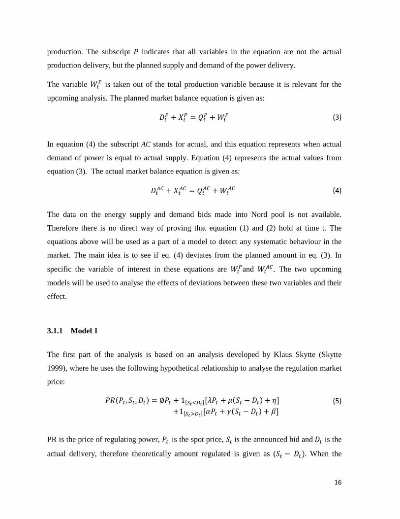
𝐷𝑡𝑃 + 𝑋𝑡𝑃 = 𝑄𝑡𝑃 + 𝑊𝑡𝑃 (3)
In equation (4) the subscript AC stands for actual, and this equation represents when actual
demand of power is equal to actual supply. Equation (4) represents the actual values from
equation (3). The actual market balance equation is given as:
𝐷𝑡𝐴𝐶 + 𝑋𝑡𝐴𝐶 = 𝑄𝑡𝐴𝐶 + 𝑊𝑡𝐴𝐶 (4)
The data on the energy supply and demand bids made into Nord pool is not available.
Therefore there is no direct way of proving that equation (1) and (2) hold at time t. The
equations above will be used as a part of a model to detect any systematic behaviour in the
market. The main idea is to see if eq. (4) deviates from the planned amount in eq. (3). In
specific the variable of interest in these equations are 𝑊𝑡𝑃and 𝑊𝑡
𝐴𝐶. The two upcoming
models will be used to analyse the effects of deviations between these two variables and their
effect.
3.1.1 Model 1
The first part of the analysis is based on an analysis developed by Klaus Skytte (Skytte
1999), where he uses the following hypothetical relationship to analyse the regulation market
price:
𝑃𝑅(𝑃𝑡, 𝑆𝑡,𝐷𝑡) = ∅𝑃𝑡 + 1[𝑆𝑡<𝐷𝑡][𝜆𝑃𝑡 + 𝜇(𝑆𝑡 − 𝐷𝑡) + 𝜂] +1[𝑆𝑡>𝐷𝑡][𝛼𝑃𝑡 + 𝛾(𝑆𝑡 − 𝐷𝑡) + 𝛽]
(5)
PR is the price of regulating power, 𝑃𝑡, is the spot price, 𝑆𝑡 is the announced bid and 𝐷𝑡 is the
actual delivery, therefore theoretically amount regulated is given as (𝑆𝑡 − 𝐷𝑡). When the
16
regulating power prices are known, the values of 𝑃𝑡, and 𝑆𝑡 are known, because the spot
market closes 12 hours before the actual delivery. 𝐷𝑡 , is the only unknown variable in this
regression model. When 𝑆𝑡< 𝐷𝑡 there is excess demand for power, and when 𝑆𝑡>𝐷𝑡 there is
excess supply. The key point in this hypothetical relation is that when there is an absence of
regulation, the regulating power price is equal to the spot price scaled by a factor.
Skytte estimates this factor to be equal to 1. The coefficients μ and ϒ are regarded as the
marginal regulating power price per unit of regulated power, and the coefficients λ, α, and β
are assumed to be unrelated to the amount of regulation. In the model these are interpreted as
determining, the premium paid to the regulators. This premium is paid because the regulators
have to regulate within 15 minutes of notice. Which is relatively quick compared to the spot
market, where the interval between acceptance of the bids and actual trade is at least 12
hours.
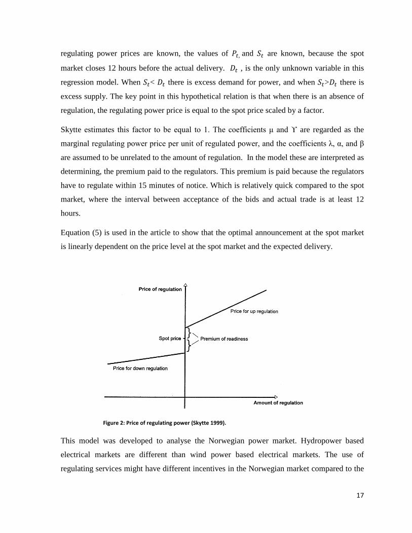
Equation (5) is used in the article to show that the optimal announcement at the spot market
is linearly dependent on the price level at the spot market and the expected delivery.
This model was developed to analyse the Norwegian power market. Hydropower based
electrical markets are different than wind power based electrical markets. The use of
regulating services might have different incentives in the Norwegian market compared to the
Figure 2: Price of regulating power (Skytte 1999).
17

Danish market. The main reason is that hydropower can to some extent be stored but such
possibilities are limited in the wind power market. This model is applied on the Danish
power market, to detect any strategic behaviour with updated data from 2012-2013.
Hereafter the model will be referred as model 1. Any asymmetries related to up and down –
regulation will be used in context with equation (1) and equation (2), and any hint of
systematic behaviour will be regarded as the variable 𝑊𝑡𝑆, the strategic element in wind
power production.
3.1.1.1 Modification of Model 1
The dataset and the generated variables used in the models is described in detail, see chapter
four. In line with the main purpose of this thesis, Model 1 is modified to approach the
analysis of the Danish market. Two dummy variables are created to modify the equation so
equation (5) can be written:
𝑃𝑅(𝑃𝑡, 𝑆𝑡,𝐷𝑡) = ∅𝑃𝑡 + �
[𝜆𝑃𝑡 + 𝜇(𝑆𝑡 − 𝐷𝑡) + 𝜂]0 [𝛼𝑃𝑡 + 𝛾(𝑆𝑡 − 𝐷𝑡) + 𝛽]
𝑖𝑓 𝑆𝑡 < 𝐷𝑡𝑖𝑓 𝑆𝑡 = 𝐷𝑡𝑖𝑓 𝑆𝑡 > 𝐷𝑡
(6)
The dummy variable for down- regulation is given by:
𝑑𝑡𝑑 = �10 𝑖𝑓 𝑆𝑡 < 𝐷𝑡𝑜𝑡ℎ𝑒𝑟𝑤𝑖𝑠𝑒
The dummy variable for up- regulation is given by:
𝑑𝑡𝑢 = �10 𝑖𝑓 𝑆𝑡 > 𝐷𝑡𝑜𝑡ℎ𝑒𝑟𝑤𝑖𝑠𝑒
With the dummy variables one has now:
𝑃𝑅(𝑃𝑡, 𝑆𝑡,𝐷𝑡) = ∅𝑃𝑡 + 𝑑𝑡𝑑[𝜆𝑃𝑡 + 𝜇(𝑆𝑡 − 𝐷𝑡) + 𝜂] +𝑑𝑡𝑢[𝛼𝑃𝑡 + 𝛾(𝑆𝑡 − 𝐷𝑡) + 𝛽]
(7)
18

Equation (7) can be rewritten as:
𝑃𝑅(𝑃𝑡 ,𝑆𝑡,𝐷𝑡) = ∅𝑃𝑡 + 𝜆�𝑑𝑡𝑑𝑃𝑡�+ 𝜇�𝑑𝑡𝑑(𝑆𝑡 − 𝐷𝑡)�+ 𝜂�𝑑𝑡𝑑�+ 𝛼[𝑑𝑡𝑢𝑃𝑡] + 𝛾[𝑑𝑡𝑢(𝑆𝑡 − 𝐷𝑡)] + 𝛽[𝑑𝑡𝑢]
Equation (7) in form of the regression model and ready for estimation becomes:
𝑃𝑅𝑡 = 𝛼0 + 𝛼1𝑃𝐷 + 𝛽0𝐷𝑢𝑝 + 𝛽1�𝑃𝐷 ∗ 𝐷𝑢𝑝� + 𝛽2�𝑉𝑢𝑝 ∗ 𝐷𝑢𝑝� + 𝛾0𝐷𝑑𝑜+ 𝛾1(𝑃𝐷 ∗ 𝐷𝑑𝑜) + 𝛾2 (𝑉𝑑𝑜 ∗ 𝐷𝑑𝑜) + 𝜀 (8)
Here, 𝑃𝑅𝑡 is the regulation price for balancing regulation and V is the actual volume of
regulation. Subscripts up and do stand for up and down- regulation. More information about
the variables is provided in chapter four.
Finally, equation (9) is studied through creating a graph. Here the change in price of
balancing regulation is given as the difference in price of up and down-regulation in the
relevant time period.
Δ𝑃𝑡𝑟 = 𝑃𝑡𝑢𝑝 − 𝑃𝑡𝑑𝑜 (9)
This modified version of Skytte's model is regarded as model 1 hereafter, because this
version of the model is relevant for the analysis.
3.1.2 Model 2
Model 2 is based on econometric theory of measurement error in the model. The estimation
method is used because there is a suspicion of endogeneity in the model. The use of proxy
variable and the use of an instrumental variable are methods used to correct for endogeneity,
given that the OLS1 estimation may not produce good results. In this case there is a
suspicion of endogeneity in the model, related to the variable of wind power production. The
objective is to check the model for endogeneity and signs of systematic measurement error
that can be linked to strategic behaviour. In Model 2, the dependent variable in the regression
1 The method of ordinary least squares
19
is total regulation, and the independent variables are net exports, wind power production and
total power production. The failure of meeting total demand at the time of actual delivery is
reflected in total regulation. The goal is to extract the effect of planned wind power
production on total regulation.
When there is endogeneity in the independent variables, the results will be produced with
bias estimates. Endogeneity can be caused by omitted variables, measurement error or
simultaneity. Possible ways to correct for unobserved endogeneity is to find a suitable proxy
for the unobserved variable. The instrumental variables regression approach can also be
applied. The use of OLS in presence of endogeneity will lead to a correlation between the
explanatory variables and the error term, and results will be biased. In this case, the
unobserved part of the model is the strategic element added to the planned wind power
production. The assumption is that this strategic element will be detected through the
endogeneity in the independent variable and this can be classified as systematic measurement
error (Reichstein 2011).
The assumption in the classical linear regression model is that the model is being measured
with an error term 𝜀. The problem of measurement error distinguishes from the error term 𝜀,
because the assumption here is that in addition to the error term of the model, the
independent variable is being measured with an error. The models with measurement errors
follow, the key assumption that the response variable and the predictor variables are subject
to additive measurement errors. The regression model in this case is subject to an unknown
constant, which classify the model to become a functional measurement error model (Young
2014).
In presence of a measurement error the estimation method of 2SLS2 can be applied to correct
for the error. In the model X is an independent variable, Y is dependent variable and Z is the
instrumental variable. The instrumental variable Z affects the dependent variable Y, only
through its effect on the independent variable X. (Young 2014). Two properties must be
satisfied in order to for the instrumental variable to be consistent. The instrumental variable
must be relevant and strong. In order to be relevant, there must be a strong correlation
2 Two-stage least-squares
20

between the IV and the independent variable it is instrumenting for. The IV must be
uncorrelated with the error term, and by that, the IV is exogenous (Young 2014).
The Hausman test is a specification test for measurement error with the null hypothesis of no
measurement error. Under this hypothesis, both the OLS estimator and the instrumental
variable estimators are consistent estimators in the model. The OLS will be efficient, and the
instrumental variable estimator will be inefficient if the null hypothesis is valid. On the other
hand, if the null hypothesis is rejected, the instrumental variable estimator will be consistent,
and not the OLS estimator. In brief, the Hausman test is used to compare the result from the
OLS and the 2SLS (Green 1990).
To improve OLS results, the OLS can be estimated using a proxy variable. There is
difficulties related to the measure corresponding to the variable 𝑊𝑡𝑃, but still this variable is
defined in the regression. There are observable indicators for this variable, and in this context
the variable wind prognosis, 𝑊𝑡𝑃𝑟𝑜𝑔, will be regarded as an indirect measure of 𝑊𝑡
𝑃.
Theoretically, it is highly unlikely that an improvement in the measurement will bring the
proxy closer to the variable, which it is a proxy for (Green 1990).
In context of the theory given above, Model 2 is designed. The objective of Model 2 is to
find the effect of 𝑊𝑡𝑃 on the total regulation amount. The unobservable variable 𝑊𝑡
𝑃 from
equation (1) will be measured indirectly as this information is missing. What is known is that
wind power production is solely dependent on the amount of wind that enters the system. To
analyse what happens when the supply bid is planned, wind fluctuations are considered. The
effect of planned wind power production on total regulation is the basis for the regression
estimation in Model 2.
Without the strategic element in the model, the assumption is as following:
𝑊𝑡𝑃 = 𝑊𝑡
𝐴𝐶 = 𝑊𝑡 (10)
Ideally, total regulation should be regressed against all the independent variables from
equation (4) to obtain the effect of planned wind power production on total regulation:
𝑅𝑡 = 𝛽0 + 𝛽1𝑄𝑡 + 𝛽2𝑋𝑡 + 𝛽3𝑊𝑡 + 𝜀𝑡 (11)
21

The introduction of an instrumental variable will attempt to solve the missing variable
problem, and the variable wind power prognosis is used as an instrument in the 2SLS:
𝑅𝑡 = 𝛼𝑡 + 𝑄𝑡 + 𝑋𝑡 + 𝑊𝑡𝑃𝑟𝑜𝑔 + 𝜀𝑡 (12)
To be able to compare the OLS estimation with planned wind power production included,
wind prognosis is tested as a proxy variable for actual wind power production, and equation
(13) becomes the following:
𝑤𝑡𝐴𝐶 = 𝛼 + 𝑤𝑡
𝑝𝑟𝑜𝑔 + 𝜀𝑡 (13)
The OLS estimation with a proxy variable is as showed in equation (14):
𝑅𝑡 = 𝛽0 + 𝛽1𝑄𝑡 + 𝛽2𝑋𝑡 + 𝛽3𝑊𝑡𝑃 + 𝛽4𝑊𝑡
𝑃𝑟𝑜𝑔𝑡 + 𝜀𝑡 (14)
Lastly, the Wu-Hausman test for endogeneity is applied to compare OLS and 2SLS results.
The OLS estimation and the OLS estimation with a proxy are compared using the Likelihood
ratio test. This test shows the improvements in the estimation by using a proxy variable.
3.1.3 Hypotheses and model summary
Hypothesis one: There is not a systematic relationship between regulation price, and up or down regulation
Hypothesis two: Wind power production is exogenous predictor of total regulation
Model 1 and Model 2 is applied in order to answer the problem of discussion. Model 1 is
estimated first, and if the results suggest that asymmetries are found, Model 2 continues the
research by specifically testing the relationship between total regulation and wind power
production, because the suspicion is that the asymmetries in the regulation market is caused
by the deviations between planned and actual wind power production. Hypothesis one is
tested in Model 1, and after the results are conducted from Model 1, hypothesis two is tested
in Model 2. To sum up, to state the problem for discussion the deviations between actual and
22

planned wind power production will be tested by the effect of wind power prognosis on total
regulation. Further, the direct effect on the bidding strategy cannot be obtained, as the data
on the actual bid is confidential. The way of analysing the bidding structure in this research
will be done by examining if there are any incentives for wind power producers to
systematically use the regulation market to preserve their interests in the spot market.
Significant measurement error may be indirect evidence on systematic action and therefore
Model 2 is tested for endogeneity.
23

This page left intentionally blank.
24
4 Data
The data used in the model 1 and model 2 is downloaded from energinet.dk, except the data
on wind prognosis which is downloaded from Nord Pool´s website. Energinet.dk updates the
homepage twice each day, and uses the latest data in update. The measurement unit and
currency unit for price is Euro per MWh. The data downloaded is from 01.01.2012 to
31.12.2013. Which is a total amount of 24 months and 17544 observations on an hourly
basis.
In general, the dataset the observations regard for 24 hours per day, but there is one particular
day in March reported with 23 hours. This happens because the time changes from
wintertime to summertime (Nielsen 2010). In the time period from 01.01.2012 to 31.12.2013,
these dates occur at 25th march 2012, and 31st March 2013, which lead to that the 3rd hour
was blank on these dates. The blank area in the data set is corrected for by filling in the data
from hour four. The mean value of hour 2 and 4 could also have been used, but the values of
these hours were very similar, so the mean value was not used to fill in for the missing hour.
When summertime changes to wintertime, in general one day will be calculated as 25 hours,
because the 3rd hour will be calculated twice (Nielsen 2010). In the dataset all of the
observations fit the time series setting from 1 to 24, therefore no 25th hour was observed.
4.1 The variables
All the observable variables used in Model 1 and 2 are in the dataset. The Elspot price for
DK-West (West-Denmark) is used as the price variable for DK-West bidding area. DK-West
primary and local production generates the variable of total production in DK-West. DK-
West wind production is treated as one variable, and not as a part of total production.
Upward and downward regulation for DK-West, both amount and price are important and
included in the dataset. In addition there is a price for balancing power consumption, which
in the analysis is shortened to price for balancing regulation, and this is regarded as the
25
regulation price. Down regulation values are given with a negative sign, and up regulation
values are given with positive signs. DK-West trades power with Norway, Sweden and
Germany, and data on trade with all the three countries is included to create one net export
variable in the analysis. The trade with East-Denmark is not considered in this variable.
Observations have either positive or negative values to distinguish between import and
export. A detailed description of how these variables are generated is given in chapter five.
4.2 Descriptive statistics
Descriptive statistics of all variables is presented in table 1. The standard deviation of total
regulation, net exports, wind prognosis and wind production is high compared to the other
variables. There are huge differences between the minimum and maximum values for all
variables. Up and down regulation have fewer observations than the other variables, because
the observation is done only for those hours when up and down -regulation takes place. Total
production has the highest mean value, and the mean value of the wind power production and
wind prognosis is very similar. The coefficient of variance is equal for wind power
production and wind prognosis. Total regulation has the highest value of the coefficient of
variance. The mean value of price for up-regulation is higher compared to down- regulation.
DK-West area price has a mean value between the mean values of up and down regulation
price.
26

Table 1: Descriptive statistics of the variables.
Variable N Mean Std-dev Median Min Skewness CV Max
Total regulation 17544 1.51 93.09 0.00 -704.70 0.21 61.58 714.90 Total production 17544 1498.32 662.59 1397.70 355.80 0.61 0.44 4062.40 Net exports 17544 135.83 660.31 174.80 -2226.30 -0.31 4.86 1896.30 Wind prognosis 17544 919.09 739.63 709.00 11.00 0.92 0.80 3323.00 Price of balancing 17544 37.21 23.90 34.36 -217.01 3.73 0.64 499.93 Wind production 17544 929.37 744.33 738.50 0.60 0.84 0.80 3871.10 Down regulation 5230 -82.51 80.51 -55.00 -704.70 -2.12 -0.98 -0.50 Up regulation 4492 101.97 89.48 81.10 0.40 1.57 0.88 714.90 Price for down regulation 17544 32.78 14.99 32.95 -217.01 -1.74 0.46 183.39 Price for up regulation 17544 42.08 39.31 37.67 -199.99 33.00 0.93 1999.89 Spot price DK-West 17544 37.66 35.24 36.15 -200.00 44.92 0.94 2000.00
27

This page intentionally left blank.
28
5 Estimation and analysis
All statistical analysis was conducted using the STATA3 software version 13. The data
described in chapter four was divided into two datasets, one for each model. Some variables
are repeated and appear in both datasets. For model 1 data is analysed in STATA as hourly
time series with time variable hour running from 1 to 17544. The results are established on
based on these 17544 hours only. Time series variable are tested for stationarity using the
Augmented Dickey- Fuller (ADF) unit root test are found to be stationary, see appendix 1 for
details
Model 1 is estimated first. Two dummy variables are generated one for up- regulation and the
other for down- regulation. The dummy variables are multiplied with the area price of DK-
West to generate two new variables as required in the model. The dummy variable for up-
regulation is multiplied with up-regulation volume, and similarly the down-regulation
dummy is multiplied with down-regulation volume. Model 1 requires all of these variables
for the regression analysis.
At first Model 1 is estimated using ordinary least square (OLS). Specification tests conducted
on OLS results indicate the need to control for autocorrelation and heteroscdasticity. To
control for autocorrelation and heteroscedasticy, the model was re-estimated twice following
the Newey-West procedure with HAC4 standard errors –first with 24 lags and later with 48
lags.
The difference between up-regulation and down-regulation prices is computed to determine
the spread in these prices. The distribution of these prices and their spread are graphed to
show the asymmetries in their distribution. The graph is showed in chapter 6.1
The analysis for Model 2 requires the variables total production, wind power production, net
exports, and total regulation, all of which are generated except wind power production. Total
regulation is generated as an aggregated value of up and down regulation. The variable net
export is generated as an aggregated value of imports and exports of DK-West with Sweden,
3 Data analysis and statistical software version 13 4 Heteroscedasticity and Autocorrelation consistent Standard Errors.
29

Norway and Germany. To generate the total power production primary production and local
production added together.
Total regulation is regressed against wind power production, total production and net exports.
Specification tests the Ramsey-Reset, the Linktest, White´s test and the Breusch-Pegan test
are applied to estimated OLS models one excluding and the other including wind power
prognosis. All specification test results indicate that OLS estimation without wind prognosis
misspecified. A second OLS model is estimated with wind power prognosis as proxy to
correct the potential missing variable problem suspected to be causing the detected
misspecification. The same four tests are applied on the OLS estimation with a proxy and
misspecification is detected to persist
Model 2 is further estimated using instrumental variable two stage least squares approach
using wind prognosis as an instrument for wind production, which suspect to be measured
with error. Tests for a good instrument F-tests and correlation are conducted on wind
prognosis assuming total production and net exports to be exogenous. Results from the
Durbin and Wu-Hausman tests in the first stage of the 2SLS approach indicate that the
instruments used are strong and relevant.
In the 2SLS total regulation is regressed against net exports, total production as exogenous
variable and wind power prognosis as an instrument for wind production as discussed in the
first stage. To compare the results of the OLS and the OLS with the proxy the likelihood ratio
test is applied. Likewise OLS results are compared with 2SLS results to detect a difference,
which points the possibility of measurement error by applying the Wu-Hausman test.
30

6 Results and discussion
This chapter provides detailed results obtained from estimation and analysis described in
chapter five. Results from Model 1 are presented first, and results from Model 2 second.
Results from both models are discussed at the end of this chapter.
6.1 Results Model 1
Table 2 provides the overview of the estimated parameters on Model 1.
Table 2: Estimated parameters model 1.
OLS NEWEY: 24 lags NEWEY: 48 lags Dependent variable: Price of balancing regulation b/se b/se b/se Area price West Denmark 0.933*** 0.933*** 0.933*** (0.009) (0.011) (0.011) Up regulation dummy -15.295*** -15.295* -15.295* (5.042) (8.061) (8.316) Up regulation price 0.468*** 0.468** 0.468** (0.115) (0.181) (0.185) Volume traded on up regulation 0.148*** 0.148*** 0.148*** (0.009) (0.017) (0.017) Down regulation dummy 26.844*** 26.844*** 26.844*** (0.782) (1.569) (1.588) Down regulation price -0.885*** -0.885*** -0.885*** (0.020) (0.040) (0.041) Volume traded on down regulation
0.048*** 0.048*** 0.048***
(0.004) (0.006) (0.007) Constant 0.981*** 0.981*** 0.981*** (0.283) (0.367) (0.373) Number of observations N = 17544 N = 17544 N = 17544 F –Statistics R-Squared
3165.81 (0.000) 0.5990
1467.90 (0.000)
1438.33 (0.000)
***, ** and * implies significant at 1%, 5% and 10% critical levels respectively
31

The OLS, Newey (24) and Newey (48) are significant at 1 %, 5% and 10 % critical level.
The R-squared value indicate that the variation in the independent variables used to estimate
Model 1, explains approximately 60 % of the variation in the balancing price of regulation.
The two-tail p-values confirm the hypothesis that each coefficient is significantly different
from 0, at 1 %, 5 % and 10 % critical levels. The estimated coefficient spot price DK-West is
significant and with a positive sign. This indicates that the balancing market follows the
signals of the spot market. The price of balancing regulation is positively related to the spot
price, if the spot price increases the balancing price increase. This is a clear indication that
the balancing price of regulation is not independent from the spot price of DK-West. In the
table this variable is called Area price West Denmark.
The estimated dummy variable for up-regulation, which in Model 1 is given by the
coefficient 𝛽0, has a negative sign. Therefore the price of balancing regulation and the
estimated dummy variable move in the opposite direction. The results are opposite for the
down-regulation dummy variable, given by the coefficient 𝛾0, which in Model 1, which has a
positive sign. This could possibly imply stabilizing effects of the up and down regulation.
When there is up regulation power supply increases in the market, and when supply increases
the demand is closer to being satisfied, and price will eventually decrease. The same
interpretation applies for down-regulation, because when down-regulation occurs, power
supply is either withdrawn from the system or at least there is no increase in supply in the
system, which will eventually lead to a price increase. The interpreted chain of events is not
reflected as a result in one single hour of delivery, but for the interval from 12 to 36 hours of
actual delivery of power.
The estimated dummy variable for up-regulation multiplied with the area price DK-West has
a positive sign. The price of balancing regulation and this estimated variable are positively
correlated, which means that, during up-regulation an increase the area price DK- West will
imply an increase in price of balancing regulation. They are both positive and move in the
same direction when a unit change occurs. A possible explanation can be that the area price
is positively correlated with the price of balancing regulation, therefore the spot price
multiplied with the dummy variable has a positive net impact. When the down regulation
dummy is equal to 1, the dummy variable is multiplied with the spot price, and this relation
32

has a positive sign. If regulation does not occur at all, zero multiplied with the spot price, will
have no effect. The estimated dummy variable for down-regulation multiplied with the area
price of DK-West is negatively correlated to the price of balancing regulation. The estimated
coefficient is significant, but the price of balancing regulation and the coefficient move in the
opposite direction. When there is a unit decrease in the estimated coefficient, there will be an
increase in the price of balancing regulation.
The coefficient 𝛽2, which represents the dummy variable for up-regulation multiplied with
the volume of up regulation, is significant with a positive sign. This is in agreement with the
economic theory, which means that there is an increased cost. When the regulating power
volume increases, the price of balancing regulation increases, and this represents the
increased cost reflected in the increased price of balancing regulation. When regulation
volumes increase, the price for balancing regulation increases. The dummy variable picks up
the frequency of up regulation, and the volume times the frequency affects the price for
regulation. The result is almost the same for the estimated coefficient 𝛾2 , which represents
the same relation in the case of down regulation. The volume of down regulation times the
frequency of down regulation also share a positive and significant relationship with the
balancing price. The use of regulation services is regarded as an additional cost, so the
question is if it is more beneficial to use this market to minimize this cost. In the next section
the difference in average price of up-regulation and down-regulation is graphed in order to
compare the skewness and over all difference in average prices.
6.1.1 The average price of up-regulation and down-regulation
The variable price of down-regulation has a left skewed distribution, which means that the
values are mostly on the right side of the mean. The opposite is valid for the price of up-
regulation, where the distribution is right skewed. There are asymmetries in the distribution
of both variables. Figure 3 below shows average price difference of up and down regulation.
The graph representing hourly averages of up and down regulation prices is the result of eq.
(9) given in Model 1. The top graph shows the hourly average, while the graph below
33
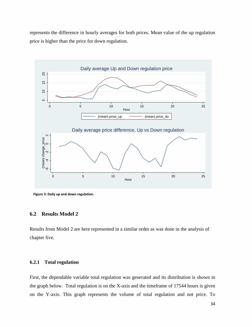
represents the difference in hourly averages for both prices. Mean value of the up regulation
price is higher than the price for down regulation.
6.2 Results Model 2
Results from Model 2 are here represented in a similar order as was done in the analysis of
chapter five.
6.2.1 Total regulation
First, the dependable variable total regulation was generated and its distribution is shown in
the graph below. Total regulation is on the X-axis and the timeframe of 17544 hours is given
on the Y-axis. This graph represents the volume of total regulation and not price. To
510
1520
0 5 10 15 20 25Hour
(mean) price_up (mean) price_do
Daily average Up and Down regulation price
-6-4
-20
2(m
ean)
cha
nge_
pric
e
0 5 10 15 20 25Hour
Daily average price difference, Up vs Down regulation
Figure 3: Daily up and down regulation.
34

distinguish between up and down-regulation, a positive sign is given to the amount of up
regulation, and a negative sign is given to the down-regulation amount in the data set. The
bell shaped curve indicates a normal distribution, but most of the observations are around a
value of zero. The minimum value of total regulation is -704.7 and the maximum value is
714.9. The median value is zero and the mean value is 1,51 and there is a right skewed
distribution with a value of 61.58, (see Table 1). Based on the descriptive statistics most of
the values are to the right of the mean. This would imply that up-regulation dominates the
distribution, because up-regulation regard for all the positive values. However, by looking at
the graph, the most frequent value is just below zero. This value is negative and all negative
values imply that there is down-regulation. This implies a contradiction in the results. A
possible explanation can be that down-regulation happens frequently but in smaller
quantities, and the volume of up-regulation is higher each time. That in turn causes the mean
value of total regulation to become positive.
Figure 4: Distribution of the variable total regulation.
35
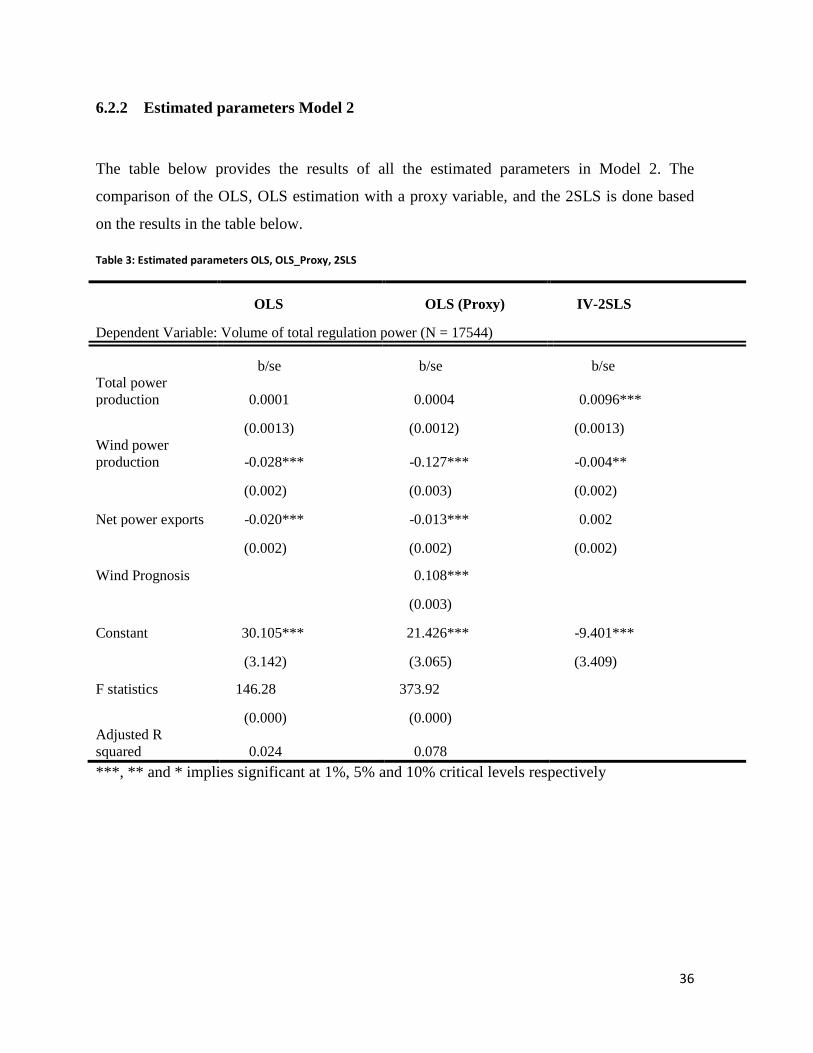
6.2.2 Estimated parameters Model 2
The table below provides the results of all the estimated parameters in Model 2. The
comparison of the OLS, OLS estimation with a proxy variable, and the 2SLS is done based
on the results in the table below.
Table 3: Estimated parameters OLS, OLS_Proxy, 2SLS
OLS OLS (Proxy) IV-2SLS
Dependent Variable: Volume of total regulation power (N = 17544)
b/se b/se b/se Total power production 0.0001 0.0004 0.0096***
(0.0013) (0.0012) (0.0013) Wind power production -0.028*** -0.127*** -0.004**
(0.002) (0.003) (0.002)
Net power exports -0.020*** -0.013*** 0.002
(0.002) (0.002) (0.002)
Wind Prognosis 0.108***
(0.003)
Constant 30.105*** 21.426*** -9.401***
(3.142) (3.065) (3.409)
F statistics 146.28 373.92
(0.000) (0.000) Adjusted R squared 0.024 0.078 ***, ** and * implies significant at 1%, 5% and 10% critical levels respectively
36
6.2.3 OLS estimation with wind power production
OLS estimation showed that the coefficient of total production is not significant. Wind power
production is negatively correlated with total regulation. Both wind power production and net
exports have negative signs, which means that when net exports and wind power production
decrease by one unit, the total regulation increases by one unit. The adjusted R-squared value
is low, approximately 2 %, therefore based on this value no significant conclusions can be
made.
The Ramsey-reset test rejected the hypothesis of no omitted variables with a p-value of 0.00.
The model is concluded as misspecified. Heteroscedasticity is detected by the White's test, a
possible way to correct for heteroscedasticity was to use robust standard errors, but even if
they had been used, model misspecification would remain. Heteroscedasticity was confirmed
with a chi-square value of 327.22 and a p-value of 0.00. Breusch-Pegan test rejected the
hypothesis of constant variance in the error term based on a chi-square value of 144.18 and
p-value of 0.00. The Linktest applied on the OLS concluded with sign of missing variables in
the model, because the squared component is significant with a p-value of 0.00, see appendix
2 for details of specification tests.
OLS estimation seems to produce biased results, and there is a strong suspicion of
endogeneity, due to unforeseen systematic behavior. An indication of this is given by the
results of Model 1. A possible explanation is that there could be a missing variable that
enhances the ability to predict wind power production. This ability may be linked to strategic
behaviour or possibly a measurement error in wind production. OLS estimation with a proxy
variable, and then the 2SLS approach is used to check for better results.
6.2.4 Wind prognosis as a proxy variable
Planned wind power production is not observable at the time when the bid is placed. Using
OLS estimation, wind power prognosis is assumed to be a good proxy for the actual wind
37
power production, because the partial regression coefficient is 0.9621. There is therefore a
strong but not perfect correlation between them, see appendix 3 for details.
When the proxy variable was included in the OLS, the R-squared value increased to become
8 %. This value is still regarded as low. The Ramsey-Reset test still classifies the model as
misspecified, with significant p-value of 0.00. Heteroscedasticity was confirmed by the
White's test and there was not any improvement in results from the Linktest, as the predicted
component squared is still significant.
The Breushc-Pegan test showed improvement in the variance of the error term. The chi-
square value of the test is 0.89, followed by a p-value of 0.3465. This is the only evidence of
the slight improvement from the OLS estimation without a proxy variable. There are still
signs of misspecification possibly due to measurement errors in the independent variables.
The likelihood ratio test concludes that OLS and OLS with proxy gave different results.
There is a slight change in the estimated coefficients, but introducing a proxy does not
improve the overall result since the model is still misspecified and there are signs of missing
variables. Even if the estimates improve slightly in magnitude, the model remains
misspecified and therefore there is not a substantial change in the results.
Using wind prognosis, as proxy variable does not solve model misspecification, therefore
there is still suspicion of endogeneity. A possible explanation is that the missing variable is
related to the planned wind power production and its effect on total regulation. The next
method applied to the problem is the 2SLS.
6.2.5 The instrumental variable approach
The criteria for using an instrumental variable is met, the F-value of 56560.86 shows that the
instrument can be regarded as a strong instrument. The correlation between wind power
production and wind power prognosis is 0.9621, which means the variables are strongly
correlated, see appendix 3. The positive relationship between wind power production and
wind power prognosis is the first stage of the 2SLS, see appendix 2 for details.
38
The results in the 2SLS indicate that there is a negative relationship between total regulation
and the instrumental variable. One may interpret this as planned wind power production
given by the wind power prognosis and total regulation is negatively related. The coefficient
of net exports is not significant. Total power production has a positive sign and is significant.
The unit change in total production will lead to a unit change in total regulation, both in the
same direction. Wind prognosis and total regulation move in opposite directions, if wind
prognosis shows an increase, the volume of total regulation will decrease. These values have
a lagged relationship, and the aim is to find an instrument for planned wind power
production, which in this case is the wind power prognosis. To compare the OLS and 2SLS,
the Wu-Hausman test is applied, which confirmed endogeneity, see appendix 2.
The Wu-Hausman test rejected that wind power production is an exogenous variable. The
OLS, OLS with a proxy or the 2SLS are all estimated with a problem of measurement. The
IV-regression does not correct for the mistakes in the OLS and OLS with a proxy variable.
6.2.6 Measurement error
Comparing the OLS results with the IV regression in the Wu- Hausman concludes that the
null hypothesis is rejected and wind power production is endogenous. The instrumental
variable approach does not correct for the endogeneity problem. The same result is obtained
by comparing the OLS results with the OLS estimation with the proxy variable. All of the
tests in Model 2 confirm the same thing; there is a measurement error in the model. There is
endogeneity in the model. Using the wind prognosis as a proxy variable does not solve the
model misspecification problem. The cause of endogeneity can also be a missing variable.
This indicates unforeseen systematic behaviour, because wind power production should be an
exogenous predictor of total regulation.
6.3 Discussion of results
The main findings in Model 1 imply that the spot market signals the regulation market,
because there is a significant relationship between the spot price and the regulation price. The
39

average regulation price is reflected in the constant term, which is the regulation price that is
independent of any other factor. If the estimated coefficient values are substituted into
equation 8 of Model 1, the results are as following:
𝑃𝑅𝑡 = 0,98 + 0,93𝑃𝐷 + (– 15,3)𝐷𝑢𝑝 + 0,47�𝑃𝐷 ∗ 𝐷𝑢𝑝� + 0,15�𝑉𝑢𝑝 ∗ 𝐷𝑢𝑝� + 26,84𝐷𝑑𝑜+ (– 0,85)(𝑃𝐷 ∗ 𝐷𝑑𝑜) + 0,048(𝑉𝑑𝑜 ∗ 𝐷𝑑𝑜) + 𝜀
Hence, the effect of up- regulation and price when all other factors held constant is given as:
𝑃𝑅𝑡 = 0,98 + 0,93𝑃𝐷 + (– 15,3)𝐷𝑢𝑝 + 0,47�𝑃𝐷 ∗ 𝐷𝑢𝑝�
𝑃𝑅𝑡 = 0,98 − 15,3 + (0,93 + 0,47)𝑃𝐷
𝑃𝑅𝑡 = −14,32 + 1,4𝑃𝐷
And the effect of down- regulation and price when all other factors held constant is:
𝑃𝑅𝑡 = 0,98 + 0,93𝑃𝐷 + 26,84𝐷𝑑𝑜 + (– 0,85)(𝑃𝐷 ∗ 𝐷𝑑𝑜)
𝑃𝑅𝑡 = 0,98 + 26,84 + (0,93 − 0,85)𝑃𝐷
𝑃𝑅𝑡 = 27,82 + 0,08 𝑃𝐷
1,4𝑃𝐷 − 0,08 𝑃𝐷 = 1,32
Findings indicate that price of using up-regulation services is higher than the price of using
down-regulation services. A higher price of up-regulation means a higher cost for producers
frequently use up-regulation services. The effects of up and down -regulation are not the
same. The possibilities of joint optimisation as discussed in chapter two and three are present.
If the price and effects of up and down regulation were the same, such possibilities would be
limited. Assume that wind power producers have a marginal cost of production close to zero
and when the market price is positive, they bid the entire amount above or equal to their
marginal cost. Then supply is bid based on the planned wind power production, which is
most likely based on the wind prognosis. The deviation between planned and actual
production can have very different consequences in the regulation market. In periods with
excessive amounts of wind, the use of the regulation market will be cheaper compared to
40
periods with little wind. This is a very clear incentive to systematically bid less supply than
the wind power prognosis on the spot market. In this manner they will need to buy down-
regulation services. These results are in line with Skytte's findings (Skytte 1999). With this
analysis it can only be stated that there is an incentive present to systematically bid on the
spot market because of the asymmetric price relation. The daily difference in average prices
of up and down-regulation are asymmetrically distributed and therefore the price difference
is of significance. The deviation between predicted and actual production of wind power
could work as an incentive to strategically place the supply bid on the spot market, and
optimize the use of regulation services. There might be a strategic incentive to systematically
bid less power supply at the spot market to obtain a reduced regulation price.
The total regulation variable has a positive mean value, and a median valued zero. However
the most frequent value was below zero according to the graph. This strengthens the
argument that a frequent use of down-regulation occurs. The amount must have been small
every time that it did not affect the mean value to become negative, and possibly every time
they up-regulate the volume has higher compared to when they down-regulate. Contradiction
between the graph and the statistics indicate that there is systematic and frequent use of
down-regulation services. To state if they strategically bid less as systematic action is
difficult to state without the additional information of the actual supply bid into Nord Pool.
The results indicate that the incentive of strategic behaviour on the spot market is present,
and therefore WtS is not equal to zero in equation (2) and planned wind power production is
determined by wind power production supply bids and the strategic element related to wind
power.
Ideally, planned wind power production and actual wind power production would be the
same, and there would not be any systematic use of the regulation market. Thus wind power
prognosis would have been 100 % accurate and no deviations would have taken place. In
reality this is very challenging to obtain.
When Model 2 was estimated the assumption was that actual wind power production is an
exogenous independent variable in predicting total regulation. As seen from specification
tests results, wind power production variable included in the OLS produced biased results
due to possible missing variables or measurement error problem. Then planned wind power
41
production, wind power prognosis is used as a proxy variable alongside actual wind power
production when the OLS was estimated again. Now results were noticeably different
compared to the OLS without a proxy but the specification tests did not improve
substantially. The results from instrument variable 2SLS estimation indicate wind power
production to be endogenous in predicting total regulation. There is a very strong indication
of measurement error in the model. Significant measurement error could be indirect evidence
on systematic action of strategic behaviour. The findings imply that the incentive to act
strategically is present, and in addition to that finding there is an unforeseen measurement
error in the model.
On the basis of the results from Model 2, one may significant systematic unforeseen
behaviour. The regulation market and the spot market are supposed to be treated as two
separate markets. Systematic use of the regulation market may encourage gaming strategies,
and collusion among the wind power producers.
However, there are several limitations in the provided analysis. No cross validation has been
done and hence these findings are only valid for these 24 months. The models are not
validated outside the sample. The analysis for the long -run may produce completely
different results. Another limitation is that this analysis is based on indirect evidence. If there
was data available on the actual bidding amount submitted to Nord Pool, this analysis may
possibly show different results. An analysis done directly using actual bidding data may lead
to different results, as there would be direct evidence for the findings. The chain of events in
the energy market are very strongly linked to each other, meaning that there may be factors
present which have not been considered in the analyssi, such as consumer aspect, seasonal
variation in demand, and the retailers role all together. This research focused only on the
production side of the market, which may not be a complete picture. One important thing in
this respect is that the regulation market is not only used by wind power producers, while the
in the analysis there is an assumption that conventional power producers can control their
production. In reality, wind power producers in often struggle with anticipating their actual
production amount.
In the event that Denmark decides to pursue its plans of increasing its wind power
production, several aspects of this analysis may be relevant. The cost structure of wind power
42

producers must be taken into consideration when more actors will enter the market. The
interests of Nord Pool, the regulation market and the wind power producers must be taken
into consideration when dealing with increased wind power in the system. In addition large
investments are required to expand the wind power sector. The investment plans bring
forward higher uncertainty and in addition to that if the strategic use of the regulation market
adds up as a factor of economic inefficiency the plans must be evaluated very carefully.
To sum up, the findings in Model 1 rejected the first hypothesis, because there is a difference
in price for up-and down regulation, and the use of the regulation market is asymmetric. The
findings in Model 2 rejected the second hypothesis, and wind power production is an
endogenous variable when predicting the total regulation amount. The deviation between
planned and actual production of wind power can be used as an incentive to place the supply
bids strategically on the spot market, to obtain a better price in the regulation market. This
behaviour distinguishes from mark-up and capital-withdrawal strategies as discussed in
chapter 2.3.1. The effect using the regulation market strategically may not have a direct
effect on the demand and thus may not affect consumers at all. Whether this type of incentive
leads to economic inefficiency or not, cannot be stated without collecting substantial
evidence and data for the long run.
43

This page intentionally left blank.
44

7 Conclusions
The objective of this study was to test for systematic relationship between up and down-
regulation and price for regulating power. Results imply that the deviation between predicted
production and actual production of wind power could work as an incentive to strategically
submit supply bid at the spot market, and optimize the use of regulation services because of
the higher cost of up-regulation compared to down-regulation. This incentive can lead the
producers to place a bid lower than the actual production, to avoid the use of up-regulation
services. In addition the results also implied that there was a frequent use of down-regulation
services even if the mean value of the observations was positive, and related to up-regulation.
Since the spot price effect the total regulation price, the cost of regulation can be anticipated
before the actual delivery of power. The second analysis concluded that wind power
production was endogenous in predicting total regulation and the instrument of wind
prognosis did not correct for endogeneity. Actual wind power production should be equal to
planned wind power production and therefore be exogenous in predicting total regulation. An
unobservable strategic element may have been added to the supply bid and comes up in the
model as a systematic measurement error.
For further research it is recommended to analyse whether strategic bidding behaviour will
lead to externalities associated with wind power production in the future. If it turns out that
strategic use of the regulation market is revealed in the long run, then some improved bidding
structure should be suggested for producers of wind power that will decrease the
opportunities to use the regulation market strategically.
45

References
Danish Wind Industry Association. (2014). WIND ENERGY: Denmark DK. Available at: http://denmark.dk/en/green-living/wind-energy/ (accessed: April 20).
Dr. Petrov, D. K., Dr. Scarsi, G. C. & van der Veem, W. (2003). Modelling Strategic Bidding Behavior In Power Markets. Eropean Electricity Markets (September 2003).
Energinett.DK. (2014). Available at: https://www.energinet.dk/EN/Sider/default.aspx. Forbes, K. F., Stampini, M. & Zampelli, E. M. (2007). Wind Power and the Electricity Market for
Upward Regulation: Evidence for Western Denmark. USAEE. Green, H. W. (1990). Econometric Analysis. Second ed.: Macmillan Publishing Company. Jensen, T. K. & Sørensen, R. Z. (2014). Facts and numbers: Danish Energy Agency. Available at:
http://www.ens.dk/en/supply/renewable-energy/wind-power/facts-about-wind-power/facts-numbers (accessed: 20 March).
Kanter, J. (2012, January 22, 2012). Obstacles to Danish Wind Power. The New York Times. Lentz, A. H. & Strandmark, L. (2014). Danish Climate and Energy Policy: Danish Energy Agency.
Available at: http://www.ens.dk/en/policy/danish-climate-energy-policy (accessed: April 10).
Nielsen, B. (2010). Introduktion til udtræk af markedsdata: Energinet.DK. Nord Pool. (2014a). The Nordic Electricity Exchange and The Nordic Model for a Liberalized
Electricity Market. 19 (accessed: 20.01.2014). Nord Pool. (2014b). Price Formation in Nord Pool Spot: Nord Pool. Available at:
http://www.nordpoolspot.com/How-does-it-work/Day-ahead-market-Elspot-/Price-formation-in-Nord-Pool-Spot/.
NordPool. (2013). History: Nord Pool Spot. Available at: http://www.nordpoolspot.com/About-us/History/ (accessed: April 15).
Reichstein, T. (2011). Econometrics Endogeneity: Department of Innovation and Organizational Economics Copenhagen Business School. 45 pp.
Skytte, K. (1999). The regulating power market on the Nordic power exchange Nord Pool: an econometric analysis. Energy Economics, 21: 14.
Young, D. (2014). Chapter 13: Measurement Errors and Instrumental Variables Regression: Pennsylvania State University Available at: https://onlinecourses.science.psu.edu/stat501/node/200 (accessed: March 2014).
46
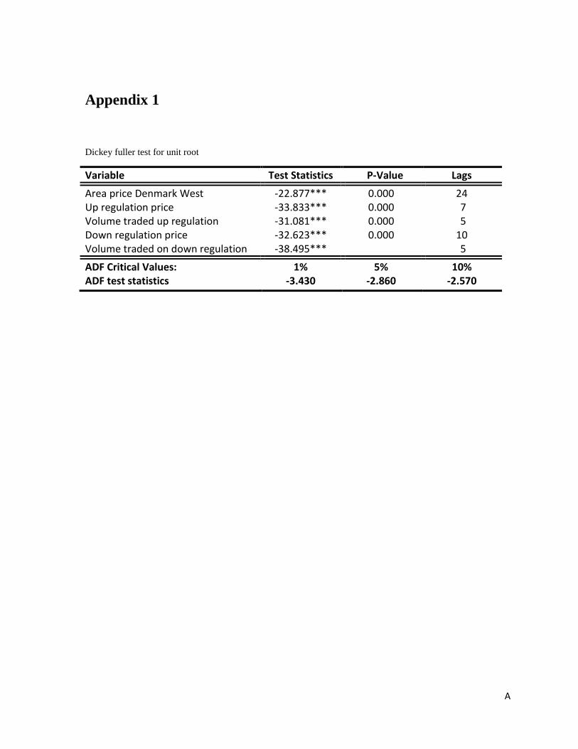
Appendix 1
Dickey fuller test for unit root
Variable Test Statistics P-Value Lags
Area price Denmark West -22.877*** 0.000 24 Up regulation price -33.833*** 0.000 7 Volume traded up regulation -31.081*** 0.000 5 Down regulation price -32.623*** 0.000 10 Volume traded on down regulation -38.495*** 5
ADF Critical Values: 1% 5% 10% ADF test statistics -3.430 -2.860 -2.570
A

This page intentionally left blank.
B
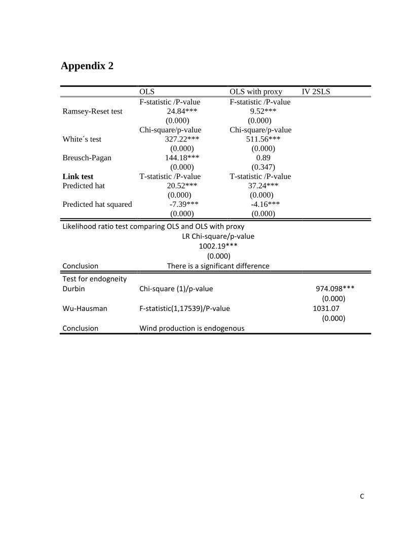
Appendix 2
OLS OLS with proxy IV 2SLS
F-statistic /P-value F-statistic /P-value
Ramsey-Reset test 24.84*** 9.52***
(0.000) (0.000)
Chi-square/p-value Chi-square/p-value White´s test 327.22*** 511.56*** (0.000) (0.000) Breusch-Pagan 144.18*** 0.89 (0.000) (0.347) Link test T-statistic /P-value T-statistic /P-value Predicted hat 20.52*** 37.24*** (0.000) (0.000) Predicted hat squared -7.39*** -4.16*** (0.000) (0.000) Likelihood ratio test comparing OLS and OLS with proxy LR Chi-square/p-value 1002.19*** (0.000) Conclusion There is a significant difference
Test for endogneity Durbin Chi-square (1)/p-value 974.098*** (0.000) Wu-Hausman F-statistic(1,17539)/P-value 1031.07 (0.000) Conclusion Wind production is endogenous
C

Test for suitability of wind prognosis, net exports and total production as good instruments for wind production
D
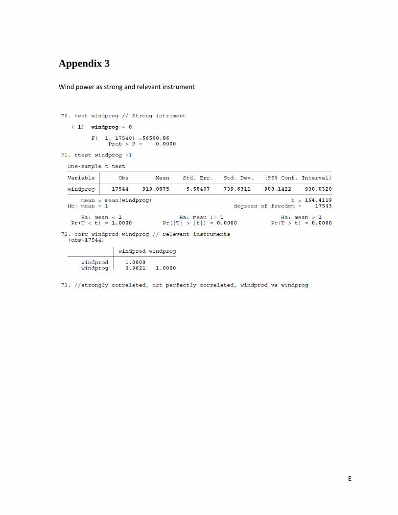
Appendix 3
Wind power as strong and relevant instrument
E

Postboks 5003 NO-1432 Ås, Norway+47 67 23 00 00www.nmbu.no

![Danish Wind Power Academy 2016 - Vestas training / Siemens ... Presentation 2016 GB.pdf · [Module index END] Page Technical training for the wind turbine industry DWPA Presentation](https://img.pdfslide.us/doc/110x75/5dd09866d6be591ccb61c111/danish-wind-power-academy-2016-vestas-training-siemens-presentation-2016.jpg)