A

prlcsywf©

K

clopemcbtflahum

S(

h0

Journal of Retailing 91 (1, 2015) 19–33

An Analysis of Assortment Choice in Grocery Retailing

Kyuseop Kwak a,∗, Sri Devi Duvvuri b,∗, Gary J. Russell c

a School of Marketing, Faculty of Business, University of Technology, Sydney, Australiab School of Business, University of Washington, Bothell, United States

c Tippie College of Business, University of Iowa, United States

bstract

Consumers in grocery retailing commonly buy bundles of products to accommodate current and future consumption. When all products in aarticular bundle share common attributes (and are selected from the same product category), the consumer is said to assemble an assortment. Thisesearch examines the impact of assortment variety on the assortment choice process. In particular, we test the prediction that consumers demandess variety for higher quality items. To investigate this relationship, we employ a flexible choice model, suitable for the analysis of assortmenthoice. The model, based upon the assumption that the utility of purchase of one item in an assortment depends upon the set of items alreadyelected, allows for a general utility structure across the assortment items. We apply the model to household assortment choice histories from theogurt product category. Substantively, we show that yogurt choice is affected by brand quality perceptions (quality-tier competition). Moreover,

e show that reaction to reductions in variety (number of yogurt flavors) is mediated by brand quality perceptions. Taken together, these empirical

acts paint a picture of a consumer who is willing to trade-off variety against product quality in assortment choice. 2014 New York University. Published by Elsevier Inc. All rights reserved.

ultiva

ta

V

cttsduac

eywords: Assortment choice; Variety; Quality perceptions; Bundle models; M

Introduction

For frequently purchased products such as grocery items,onsumers can more easily anticipate short-run preferences thanong-run preferences (Kahneman and Snell 1990; Luce 1992). Inrder to balance the trade-off between short-term and long-termreferences, consumers assemble bundles of products duringach shopping trip. Of particular interest is the product assort-ent, a bundle consisting of items selected from a single product

ategory (such as breakfast cereals or yogurt). From a choiceehavior perspective, assortments allow consumers to buy goodshat will be consumed over time. This provides the consumerexibility in planning for future consumption events and inccommodating the preferences of multiple users in the house-

old (Chernev 2011). From a retail management perspective,nderstanding the consumer decision process behind assort-ents provides guidelines for the number and variety of items

∗ Corresponding author.E-mail addresses: Kyuseop.kwak@uts.edu.au (K. Kwak),

DDuvvuri@uwb.edu (S.D. Duvvuri), gary-j-russell@uiowa.eduG.J. Russell).

ew

tt2h(

ttp://dx.doi.org/10.1016/j.jretai.2014.10.004022-4359/© 2014 New York University. Published by Elsevier Inc. All rights reserv

riate logistic model

hat should be stocked in a given product category (Corstjensnd Corstjens 2002).

ariety of an Assortment

An assortment can be viewed as a choice strategy that allowsonsumers to pursue multiple decision objectives. Due to theransaction costs of grocery shopping, it is more efficient forhe consumer to buy an assortment of products that will be con-umed in the future. Assortments permit consumers to minimizeecision conflict on a given trip (Simonson 1990), account forncertainty in future preference (Kahn and Lehmann 1991; Shinnd Ariely 2004; Walsh 1995), and address attribute satiation inonsumption (Kim, Allenby, and Rossi 2002). All these studiesmphasize that assortments are constructed to maximize varietyith respect to item attributes.Research in the store choice and consumer behavior litera-

ure argues that assortment variety is a psychological perception

hat plays a key role in the purchase decision (e.g., Broniarczyk008; Hoch, Bradlow, and Wansink 1999). Variety perceptionas been found to depend upon the size of the assortmente.g., Broniarczyk, Hoyer, and McAlister 1998; Kahn 1995),

ed.

2 f Reta

tMaBio(aecipo((aic

V

tpt1toqteTiv

hHmiiamtarv

M

epsttoFi

cbdpotsosgeup

aetotiwlaohfst

O

pmgwctwafca(MbTaf

0 K. Kwak et al. / Journal o

he distinctiveness of alternatives (Gourville and Soman 2005;arkman and Gentner 1993; Van Herpen and Pieters 2007),

nd the proximity and display of alternatives (e.g., Hoch,radlow, and Wansink 1999). While larger assortments are typ-

cally believed to offer greater variety, decreasing the numberf alternatives may actually increase the purchase likelihoodBroniarczyk, Hoyer, and McAlister 1998; Kahn 1995; Kuksovnd Villas-Boas 2010). This may be attributed to the time andffort trade-off consumers resort to while making grocery pur-hases (Hoyer 1984). Assortments with greater similarity amongtems are perceived to have lower variety, thus lowering therobability of purchase. However, items that are displayed (orrganized) together are often perceived to offer greater varietyChernev 2011). Factors such as the marginal utility of itemsKahn, Moore, and Glazer 1987; Kahneman and Snell 1992)nd overall assortment attractiveness (e.g., inclusion of favoritetem/brand) (Botti and McGill 2006) supplement variety per-eptions in motivating assortment preference and purchase.

ariety and Product Quality

Recent work by Chernev and Hamilton (2009) proposes aheory of choice behavior that links assortment size to perceivedroduct quality. This theory is based upon the trade-off betweenhe cognitive effort in evaluating choice alternatives (Shugan980) and the desire for more variety. Two assumptions underliehis theory. First, cognitive effort is proportional to the numberf items in the assortment, but has no relationship to perceiveduality of the items. Second, utility for item variety is assumedo be a concave function. Due to decreasing marginal returns,ach new item in the assortment adds less incremental utility.he consumer will add new items to the assortment until the

ncreasing mental costs overwhelm the added utility of moreariety.

Suppose that the consumer constructs assortments from eitherigh quality items or low quality items (not both). Chernev andamilton (2009) propose that for assortments of equal size, thearginal benefit of adding an item to a high quality assortment

s smaller than marginal benefit of adding an item to a low qual-ty assortment. The argument, in essence, is that each item of

high quality assortment is sufficiently valued that decreasingarginal returns become binding more quickly. Thus, the predic-

ion is quite simple: consumers will prefer a small high-qualityssortment over a large low-quality assortment. The goal of ouresearch is to evaluate the evidence for this relationship betweenariety and product quality.

odeling Assortment ChoiceTo test this prediction, it is necessary to construct a gen-

ral model of assortment choice. The academic literature onroduct bundles provides insights on how a model might be con-tructed. Multi-attribute models of bundle choice assume thathe researcher has a list of product attributes for each item in

he bundle and understands how these attributes interact withne another in determining consumer preferences (Rao 2004).or example, Farquhar and Rao (1976) develop a bundle util-

ty model based upon the assumption that the researcher can

fidi

iling 91 (1, 2015) 19–33

ode each attribute in terms of “more is better” (maximize theundle mean) or “heterogeneity is better” (maximize the bun-le variance). Preference for the bundle, then, reflects consumerreference for global features that are derived from the attributesf all items in the bundle. Harlam and Lodish (1995) draw uponhis global feature logic, but assume that the bundle is assembledequentially (across grocery shopping trips), with the probabilityf choosing the next product contingent on the products alreadyelected. Because order of purchase is generally not reported inrocery scanner datasets, the authors assume that higher pref-rence products are purchased earlier. More generally, bundletility models can be constructed using conjoint measurementrocedures (Green, Jain, and Wind 1972).

Although these models have many attractive features, theyre not suitable for empirical studies in a grocery shoppingnvironment. The key reason is that the researcher does notypically have an exhaustive list of product features. More-ver, it is clear that the modeling framework must be ableo simultaneously accommodate various demand relationships,ncluding complementarity and substitution. For these reasons,e model assortment choice using a version of the multivariate

ogistic (MVL) category incidence model developed by Russellnd Petersen (2000). The model implies that the probabilityf buying an assortment on a shopping trip depends upon theousehold’s valuation of each item in the assortment, adjustedor the demand relationships among the items. As we show sub-equently, the model provides a strong foundation for studyinghe linkage between product quality and assortment variety.

verview of Research

The remainder of this paper is organized as follows. We firstrovide a brief review of the multivariate logistic (MVL) choiceodel, explaining how the model can be extended to build a

eneral model of assortment choice. Drawing upon this theory,e construct an assortment choice model for the yogurt product

ategory that links product characteristics (brand and flavor) tohe pattern of household purchase decisions. This choice model,hich assumes perfect substitution across brand names and pick-

ny choice among flavors within a brand, provides a structureor studying the role of brand quality perceptions in assortmenthoice. Substantively, we show that the pattern of competitionmong yogurt items is affected by brand quality perceptionsBlattberg and Wisniewski 1989; Sivakumar and Raj 1997).

oreover, we show that reaction to reductions in variety (num-er of yogurt flavors) is mediated by brand quality perceptions.he overall pattern of our findings is consistent with the Chernevnd Hamilton (2009) theory. We conclude with suggestions foruture research.

Multivariate Logistic Model of Assortment Choice

In this section, we describe an assortment model that allows

or a very flexible pattern of product competition. The models built upon the conditional utility of choice of a single item,ependent on its own marketing mix and the other item choicesn the chosen assortment. The development here, which builds

f Reta

ucvtTea

M

tmhmtatia

1Dc

z

wtc(op

gtoitc

U

whbmu

tdFfl

eh

θ

sisi

ta

�

wc(

U

tto

P

wt

o1scoin the assortment. Note that each of the M possible items hasa full conditional distribution in the general form of Eq. (5),and all of these M models collectively describe the choice pro-cess of the household. The technical problem is to write downa global probability model that is consistent with this system ofinterlocking equations.

This problem has been analyzed and solved by researchers

K. Kwak et al. / Journal o

pon the discussion in Russell and Petersen (2000), yields ahoice model specification that is a special case of the multi-ariate logistic distribution proposed by Cox (1972). However,he model is considerably richer than the derivation implies.he model is consistent with theoretical frameworks in bothconomics and psychology, and has sufficient flexibility toccommodate complex demand patterns among items.

odel Description

We begin with a discussion of bundle choice, keeping in mindhat an assortment is a bundle of products, all of which are

embers of the same product category. Suppose that household selects an assortment b at time t. An assortment b containsultiple items (zero, one or more items) from multiple clus-

ers. We use the word cluster to mean a set of items with somettribute in common. For example, in a study of assortments inhe laundry detergent category, clusters might be submarket des-gnations (liquid detergents), family brand names (e.g., Tide), or

collection of product features (scented liquid detergents).Denote jc as an item j (= 1, 2, . . ., Jc) in cluster c (=

, 2, . . ., C). The total number of alternatives is M = ∑Cc=1Jc.

efine an assortment as a M × 1 vector of binary variables indi-ating the presence of the item in an assortment

bht =

[z1h1t , z1

h2t , . . ., z1hJ1t

, z2h1t , z2

h2t , . . ., z2hJ2t

, . . ., zChJCt

]′

(1)

here zchjt = 1 if household h selects item j in cluster c at time

, and equals zero otherwise. Under the assumption of pick-anyhoice, there are 2M possible assortments that could be selectedincluding the null assortment containing no purchases). With-ut further restriction, the model subsequently assigns a choicerobability to each of these 2M assortments.

We now define the conditional choice probability for an item,iven choices of all other items in the assortment. The condi-ional utility consists of two parts: (a) a baseline utility dependentn item characteristics and (b) demand interactions with othertems in the assortment. The utility of item j in cluster c, condi-ional on the observed purchase outcomes of other items underonsideration, is assumed to have the form

(jc|all else) = πchjt +

∑c∗

∑k

θc,c∗hjk zc∗

hkt + εhjt (2)

here πchjt is a baseline utility for item j in cluster c of household

, at time t and εhjt is a Gumbel distributed random error. Theaseline utility depends both upon household preferences andarketing mix elements, and can be regarded as the inherent

tility for the item, net of demand interactions with other items.These interactions are represented by the double summation

erm on the right hand side of Eq. (2). Individual items areenoted by the notation [c, j] for item j nested within cluster c.or purposes of model identification, we assume that θ

c,c∗hjk = 0,

or [c, j] = [c*, k] (We discuss the necessity of this restriction

ater in this section). The parameter θ

c,c∗hjk captures the influ-

nce of item [c*, k] on [c, j]. Accordingly, θc,c∗hjk > 0 if item k

as positive impact (complementarity effect) on item j’s utility,

wono

iling 91 (1, 2015) 19–33 21

c,c∗hjk < 0 if item k negatively influences item j’s utility (sub-

titution effect), and θc,c∗hjk = 0 if there is no influence between

tems (independence). For reasons that will become clear sub-equently, we require that the θ

c,c∗hjk parameters be symmetric in

tems [c, j] and [c*, k].To simplify the presentation of the model, it is useful to define

he symmetric matrix, �h, containing all the elements of θc,c∗hjk ,

s

h = [�1h1, �1

h2, . . ., �1hJ1

, �2h1, . . ., �C

hJC]′NJ×1

=

⎡⎢⎢⎢⎢⎢⎢⎣

0 θ1,1h12 · · · θ

1,Ch1JC

θ1,1h21 0 · · · θ

1,Ch2JC

......

. . ....

θC,1hJC1 θ

C,1hJC2 · · · 0

⎤⎥⎥⎥⎥⎥⎥⎦

NJ×NJ

(3)

here �chj is the column vector for the corresponding item j in

luster c of the matrix �h. Using matrix (3) and choice vector1), we can now rewrite Eq. (2) as

(jc|all else) = πchjt + �c′

hjzbht + εhjt (4)

Assuming that the error in (4) follows a Gumbel distribution,he conditional probability of purchasing item j in cluster c, givenhe known purchase outcomes for all other items, has the formf the binary logit model

r(zchjt|all other zs) = {exp(πc

hjt + �chj′zb

ht)}zchjt

1 + exp(πchjt + �c

hj′zbht)

(5)

here, as noted earlier, zchjt ∈ {0, 1} is an indicator variable repor-

ing whether or not item j is chosen.Eq. (5) is known in the spatial statistics literature as an autol-

gistic regression model (Anselin 2002; Besag 1974; Cressie993). From the standpoint of statistical theory, Eq. (5) can beeen to be the full conditional distribution of one binary pur-hase variable (corresponding to item [c, j]), given the knownutcomes of the binary purchase variables for all other items

orking in spatial statistics (Besag 1974). We provide anverview of the key results in Appendix A. As Besag (1974)otes, there exists a global probability model consistent with (5)nly when the cross-effect matrix is symmetric (θc,c∗

hjk = θc∗,chkj ).

2 f Reta

Wt

P

w

Md�csmvcdtita

coeEemtewc

iioow(twcaHbotso

aS

imamwusas

M

papd1citi

MTpiefli(mtna

ctCGtu�attii

2 K. Kwak et al. / Journal o

ith this symmetry assumption, the global choice model takeshe form

r(zht = zbht) = exp(Vhbt)∑

b∗ exp(Vhb∗t)

=exp

(�′

htzbht + 1

2

{zbht ′�hzb

ht

})∑

b∗ exp(

�′htz

b∗ht + 1

2

{zb∗ht ′�hzb∗

ht

}) (6)

here �ht =[π1

h1t , π1h2t , . . ., π1

hJ1t, π2

h1t , . . ., πChJCt

]′is a

× 1 column vector containing the individual (full) con-itional baseline utilities for items in consideration. Here′htz

bht is a summation of baseline utilities for items in the

hosen assortment b. It is important to understand that theystem of equations given by (5) implies the assortment choiceodel given by (6). That is, once the researcher assumes the

alidity of the M equations in (5), Eq. (6) follows as a logicalonsequence. Conversely, (6) implies the set of full conditionalistributions in (5). Using statistical terminology, Eq. (6) ishe joint (multivariate) distribution of the M binary purchasendicator variables zht. Because (6) is known to statisticians ashe multivariate logistic distribution (Cox 1972), we refer to (6)s the multivariate logistic (MVL) choice model.1

As discussed earlier, the cross-effect matrix �h obeys twoonstraints. First, the diagonal of the matrix is set to zero. Sec-nd, the matrix is symmetric. Both are technical restrictions tonsure that the model is properly specified. Given the form ofq. (6), it is easily shown that zeros on the diagonal of the cross-ffect matrix are necessary to allow the parameters in the �′

htzbht

ain effect terms to be identified. The symmetry restriction onhe cross-effect matrix is necessary to conclude that the set ofquations in (5) implies the global model in (6). Put anotheray, if cross-effects were asymmetric, then no global model

onsistent with Eq. (5) exists (Besag 1974).From a more intuitive point of view, the cross effect matrix

s a signed (plus or minus) measure of similarity across itemsn the assortment. In the spatial statistics literature, the elementsf an autologistic cross-effect matrix are modeled as functionsf the relative geographic distance between response locations,ith closer locations having a larger (positive) cross-effect term

Anselin 2002; Cressie 1993). Conceptually, it is useful to regardhe items in the assortment as being located on a mental map inhich closer items have stronger interactions with respect to the

onsumer’s buying behavior (Moon and Russell 2008; Russellnd Petersen 2000). The elements of �h are not correlations.owever, using the properties of the multivariate logistic distri-ution (Cox 1972), it can be shown that the correlations in choiceutcomes among the items in the assortment are determined byhe cross-effect matrix. Thus, symmetry in cross-effects is neces-

ary because of the link between �h and the correlation structuref the global choice model.

1 Marketing science applications related to the MVL model include Boztugnd Hildebrandt (2008), Moon and Russell (2008), Niraj, Padmanabhan, andeetharaman (2008), and Yang et al. (2010).

t

aiicI

iling 91 (1, 2015) 19–33

The symmetry of the cross-effect matrix also has anothernteresting interpretation. As explained in Appendix A, the MVLodel derivation assumes that the consumer’s valuation of an

ssortment depends only on the final composition of the assort-ent – not upon the order in which the items in the assortmentere actually selected. Put another way, a consumer who val-es an assortment solely on the basis of its contents must have aymmetric �h matrix. This order independence property is quitettractive in grocery retailing applications in which purchaseequence is not observed.

odel Interpretation

The MVL choice model can be viewed from a variety oferspectives. In the spatial statistics literature, the model isn example of a conditional autoregressive (CAR) stochasticrocess in which the researcher uses a set of full conditionalistributions to derive the form of a joint distribution (Cressie993). This interpretation emphasizes the fact that the localhoice behavior in Eq. (5) determines the global choice behaviorn Eq. (6). The CAR approach provides a way for the researchero specify a complex system by breaking the system into Mnterlocking parts, each of which can be developed separately.

From the standpoint of the marketing science literature, theVL choice model can be given two different interpretations.

he first interpretation treats Eq. (5) as a linkage between theurchase decision for one item and the actual choices of all othertems. Anselin (2002), in a review of the spatial econometrics lit-rature, calls the system of equations represented by (5) reactionunctions and the implied global model in (6) the system equi-ibrium. In other words, if the consumer simultaneously makesndividual item choices using a random utility process given by5), then the observed global choice behavior (for the assort-ent) will be observed to follow (6). In fact, recent work in

he marketing science literature by Yang et al. (2010) uses eco-omic theory to argue that MVL choice model in (6) represents

decision process equilibrium.The second marketing science interpretation specifies the

hoice model in (6) directly by making assumptions abouthe nature of the utility function of an assortment. Song andhintagunta (2006), using a utility theory argument due toentzkow (2007), adopt this approach. These authors make

wo key assumptions. First, they assume that the expectedtility for an assortment of goods Vhbt has the general form′htz

bht + (1/2)

{zbht ′�hzb

ht

}. Here, Vhbt can be considered to be

discrete variable second-order (quadratic) approximation tohe true (indirect) utility of assortment b. Second, they assumehat the actual utilities fluctuate around Vhbt due to independent,dentically distributed, extreme value errors. These assumptions,n the context of a random utility theory framework, also yieldhe MVL choice model in (6).

Intuitively, the MVL choice model states that the utility ofn assortment depends upon household valuations for each item

n the assortment, adjusted for interactions among the selectedtems. This theory exhibits clear relationships with work in theonsumer behavior literature dealing with product assortments.f all elements of Θh are set to zero, then Vhbt is just the sum of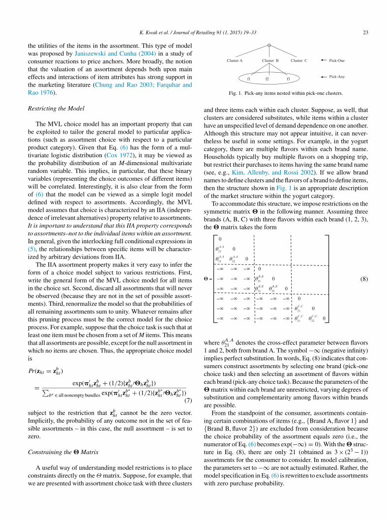

f Retailing 91 (1, 2015) 19–33 23

twctetR

R

btpttrvwodmdItI(i

fwibmatpltwi

P

sIsz

C

cw

achAtcHb(nto

sbt

Θ

w1isce�

sa

i{tnt

K. Kwak et al. / Journal o

he utilities of the items in the assortment. This type of modelas proposed by Janiszewski and Cunha (2004) in a study of

onsumer reactions to price anchors. More broadly, the notionhat the valuation of an assortment depends both upon mainffects and interactions of item attributes has strong support inhe marketing literature (Chung and Rao 2003; Farquhar andao 1976).

estricting the Model

The MVL choice model has an important property that cane exploited to tailor the general model to particular applica-ions (such as assortment choice with respect to a particularroduct category). Given that Eq. (6) has the form of a mul-ivariate logistic distribution (Cox 1972), it may be viewed ashe probability distribution of an M-dimensional multivariateandom variable. This implies, in particular, that these binaryariables (representing the choice outcomes of different items)ill be correlated. Interestingly, it is also clear from the formf (6) that the model can be viewed as a simple logit modelefined with respect to assortments. Accordingly, the MVLodel assumes that choice is characterized by an IIA (indepen-

ence of irrelevant alternatives) property relative to assortments.t is important to understand that this IIA property correspondso assortments–not to the individual items within an assortment.n general, given the interlocking full conditional expressions in5), the relationships between specific items will be character-zed by arbitrary deviations from IIA.

The IIA assortment property makes it very easy to infer theorm of a choice model subject to various restrictions. First,rite the general form of the MVL choice model for all items

n the choice set. Second, discard all assortments that will nevere observed (because they are not in the set of possible assort-ents). Third, renormalize the model so that the probabilities of

ll remaining assortments sum to unity. Whatever remains afterhis pruning process must be the correct model for the choicerocess. For example, suppose that the choice task is such that ateast one item must be chosen from a set of M items. This meanshat all assortments are possible, except for the null assortment inhich no items are chosen. Thus, the appropriate choice model

s

r(zht = zbht)

= exp(�′htz

bht + (1/2){zb

ht ′�hzbht})∑

b∗ ∈ all nonempty bundles exp(�′htz

b∗ht + (1/2){zb∗

ht ′�hzb∗ht })

(7)

ubject to the restriction that zbht cannot be the zero vector.

mplicitly, the probability of any outcome not in the set of fea-ible assortments – in this case, the null assortment – is set toero.

onstraining the � Matrix

A useful way of understanding model restrictions is to placeonstraints directly on the Θ matrix. Suppose, for example, thate are presented with assortment choice task with three clusters

atmw

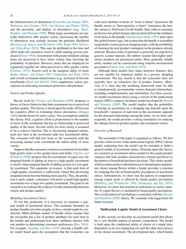
Fig. 1. Pick-any items nested within pick-one clusters.

nd three items each within each cluster. Suppose, as well, thatlusters are considered substitutes, while items within a clusterave an unspecified level of demand dependence on one another.lthough this structure may not appear intuitive, it can never-

heless be useful in some settings. For example, in the yogurtategory, there are multiple flavors within each brand name.ouseholds typically buy multiple flavors on a shopping trip,ut restrict their purchases to items having the same brand namesee, e.g., Kim, Allenby, and Rossi 2002). If we allow brandames to define clusters and the flavors of a brand to define items,hen the structure shown in Fig. 1 is an appropriate descriptionf the market structure within the yogurt category.

To accommodate this structure, we impose restrictions on theymmetric matrix � in the following manner. Assuming threerands (A, B, C) with three flavors within each brand (1, 2, 3),he � matrix takes the form

,21

, ,31 32

,21

, ,31 32

,21

, ,31 32

0

0

0

0

0

0

0

0

0

A A

A A A A

B B

B B B B

C C

C C C C

θ

θ θ

θ

θ θ

θ

θ θ

−∞ −∞ −∞

= −∞ −∞ −∞

−∞ −∞ −∞

−∞ −∞ −∞ −∞ −∞ −∞

−∞ −∞ −∞ −∞ −∞ −∞

−∞ −∞ −∞ −∞ −∞ −∞

(8)

here θA,A21 denotes the cross-effect parameter between flavors

and 2, both from brand A. The symbol −∞ (negative infinity)mplies perfect substitution. In words, Eq. (8) indicates that con-umers construct assortments by selecting one brand (pick-onehoice task) and then selecting an assortment of flavors withinach brand (pick-any choice task). Because the parameters of the

matrix within each brand are unrestricted, varying degrees ofubstitution and complementarity among flavors within brandsre possible.

From the standpoint of the consumer, assortments contain-ng certain combinations of items (e.g., {Brand A, flavor 1} andBrand B, flavor 2}) are excluded from consideration becausehe choice probability of the assortment equals zero (i.e., theumerator of Eq. (6) becomes exp(−∞) = 0). With the � struc-ure in Eq. (8), there are only 21 (obtained as 3 × (23 − 1))

ssortments for the consumer to consider. In model calibration,he parameters set to −∞ are not actually estimated. Rather, theodel specification in Eq. (6) is rewritten to exclude assortmentsith zero purchase probability.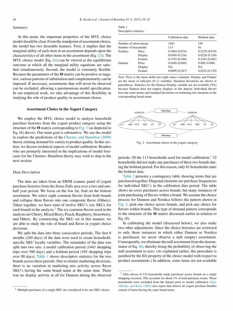

2 f Retailing 91 (1, 2015) 19–33

S

mtmcMofiBticIs

psEtttwcn

D

phaaTeaaad

msstobtSw

Table 1Descriptive statistics.

Calibration data Holdout data

Number of observations 1443 185Number of households 113 81Nordica Price 0.5464 (0.074) 0.5278 (0.070)

Display 0.0569 (0.216) 0.0226 (0.158)Feature 0.1793 (0.366) 0.2542 (0.403)

Dannon Price 0.6456 (0.049) 0.688 (0.008)Display NA NAFeature 0.0699 (0.247) 0.0222 (0.129)

Note: Price is the mean dollar per eight ounce container. Display and Featureare the mean of indicator (0–1) variables. Standard deviations are shown inparentheses. Statistics for the Dannon Display variable are not available (NA)because Dannon does not employ displays in this dataset. Individual flavorshave the same means and standard deviations on marketing mix elements as thecorresponding brand name.

phit

pfsjpFfltE

ttiCinull assortment to zero. (As explained earlier, this procedure isjustified by the IIA property of the choice model with respect toproduct assortments.) In addition, some items are not available

4 K. Kwak et al. / Journal o

ummary

At this point, the important properties of the MVL choiceodel should be clear. From the standpoint of assortment choice,

he model has two desirable features. First, it implies that thearginal utility of each item in an assortment depends upon the

haracteristics of all other items in the assortment (Eq. (2)). TheVL choice model (Eq. (6)) can be viewed as the equilibrium

utcome at which all the marginal utility equations are satis-ed simultaneously. Second, the model is extremely flexible.ecause the parameters of the � matrix can be positive or nega-

ive, various patterns of substitution and complementarity can bemposed. If necessary, assortments that will never be observedan be excluded, allowing a parsimonious model specification.n our empirical work, we take advantage of this flexibility intudying the role of product quality in assortment choice.

Assortment Choice in the Yogurt Category

We employ the MVL choice model to analyze householdurchase histories from the yogurt product category using thetructure of the � matrix corresponding to Fig. 1 (as depicted inq. (8) above). Our main goal is substantive. We use the model

o explore the predictions of the Chernev and Hamilton (2009)heory relating demand for variety to product quality. In this sec-ion, we discuss technical aspects of model calibration. Readersho are primarily interested in the implications of model fore-

asts for the Chernev–Hamilton theory may wish to skip to theext section.

ata Description

The data are taken from an ERIM scanner panel of yogurturchase histories from the Sioux Falls area over a two and one-alf year period. We focus on the low fat, fruit on the bottomssortment. We select eight common flavors from both brandsnd collapse three flavors into one composite flavor (Others).aken together, we have total of twelve SKU’s (six SKUs forach brand) in the analysis.2 The six common flavors used in thenalysis are Cherry, Mixed Berry, Peach, Raspberry, Strawberry,nd Others. By constructing the SKU set in this manner, were able to study the role of brand and flavor in yogurt choiceecisions.

We split the data into three consecutive periods. The first 8onths (240 days) of the data were used to create household-

pecific SKU loyalty variables. The remainder of the data wasplit into two sets: a model calibration period (1443 shoppingrips over 580 days) and a holdout period (185 shopping tripsver 90 days). Table 1 shows descriptive statistics for the tworands across these periods. Due to retailer marketing decisions,

here is no variation in marketing mix activity across flavorKU’s having the same brand name at the same time. Thereas no display activity at all for Dannon during the observed

2 Multiple purchases of a single SKU are considered to be one SKU choice.

shAc

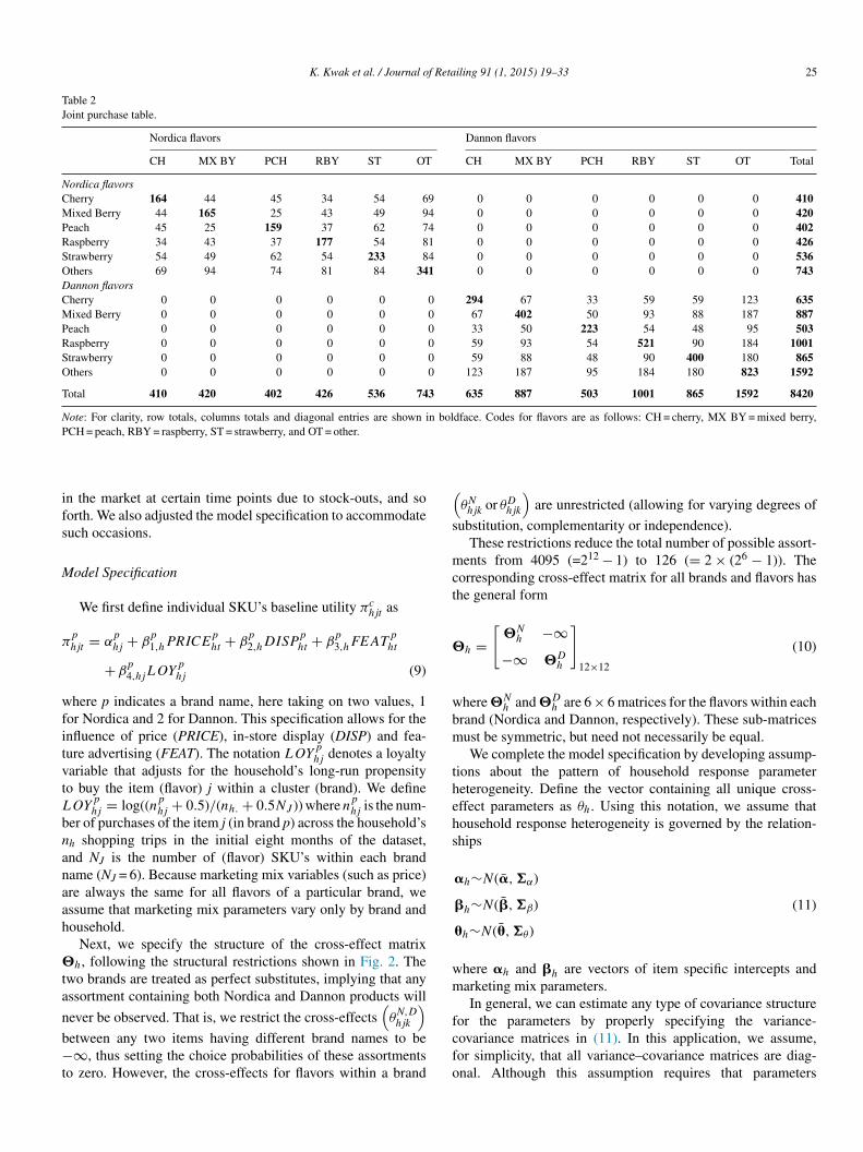
Fig. 2. Assortment choice in the yogurt category.

eriods. Of the 113 households used for model calibration,3 32ouseholds did not make any purchases of these two brands dur-ng the holdout period. For this reason, only 81 households enterhe holdout data.

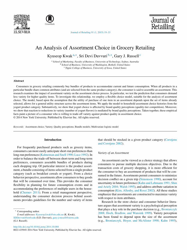
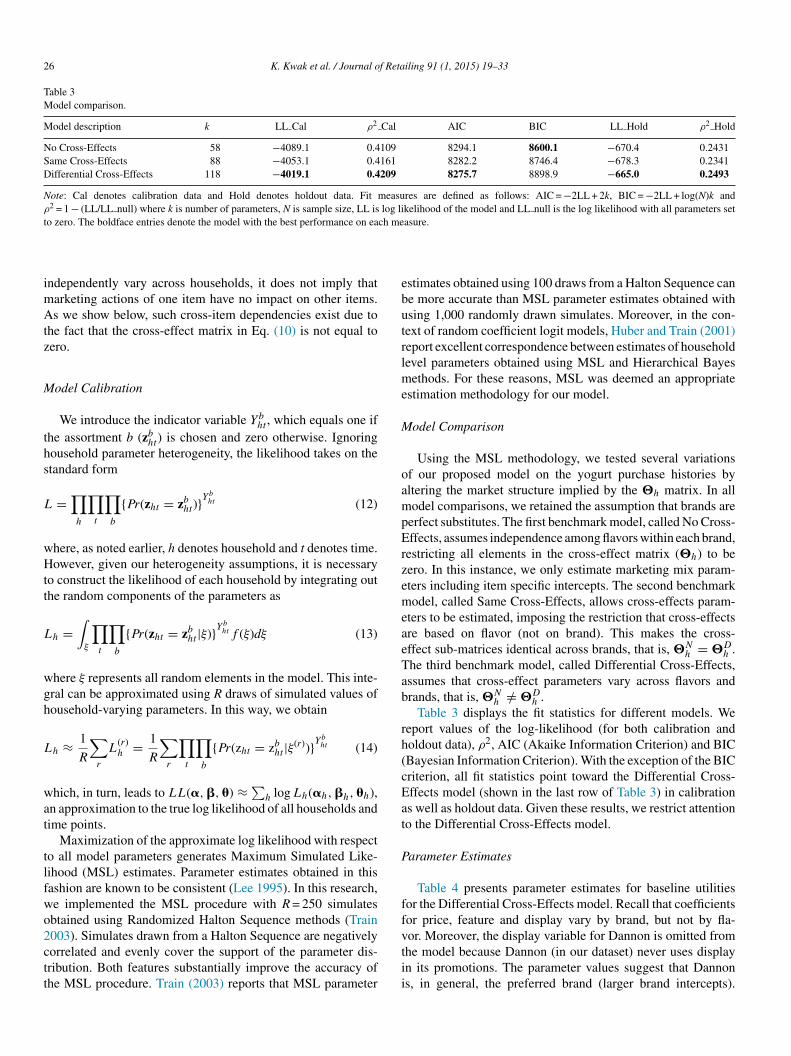
Table 2 presents a contingency table showing items that areurchased together. Diagonal elements are purchase frequenciesor individual SKU’s in the calibration data period. The tablehows no cross purchases across brands, but many instances ofoint purchasing of flavors within a brand. We assume the choicerocess for Dannon and Nordica follows the pattern shown inig. 2: pick-one choice across brands, and pick-any choice foravors within brands. This type of demand pattern corresponds

o the structure of the � matrix discussed earlier in relation toq. (8).

In calibrating the model (discussed below), we also makewo other adjustments. Since the choice histories are restrictedo only those instances in which either Dannon or Nordicas purchased, we never observe a null (empty) assortment.onsequently, we eliminate the null assortment from the denom-

nator of Eq. (6), thereby fixing the probability of observing the

3 Only eleven of 124 households made purchases across brands on a singlehopping occasion. This accounts for about 1% of total purchase events. Theseouseholds were excluded from the dataset prior to model calibration. Kim,llenby, and Rossi (2002) also report that almost all yogurt purchase bundles

onsist of items having the same brand name.

K. Kwak et al. / Journal of Retailing 91 (1, 2015) 19–33 25

Table 2Joint purchase table.

Nordica flavors Dannon flavors

CH MX BY PCH RBY ST OT CH MX BY PCH RBY ST OT Total

Nordica flavorsCherry 164 44 45 34 54 69 0 0 0 0 0 0 410Mixed Berry 44 165 25 43 49 94 0 0 0 0 0 0 420Peach 45 25 159 37 62 74 0 0 0 0 0 0 402Raspberry 34 43 37 177 54 81 0 0 0 0 0 0 426Strawberry 54 49 62 54 233 84 0 0 0 0 0 0 536Others 69 94 74 81 84 341 0 0 0 0 0 0 743Dannon flavorsCherry 0 0 0 0 0 0 294 67 33 59 59 123 635Mixed Berry 0 0 0 0 0 0 67 402 50 93 88 187 887Peach 0 0 0 0 0 0 33 50 223 54 48 95 503Raspberry 0 0 0 0 0 0 59 93 54 521 90 184 1001Strawberry 0 0 0 0 0 0 59 88 48 90 400 180 865Others 0 0 0 0 0 0 123 187 95 184 180 823 1592

Total 410 420 402 426 536 743 635 887 503 1001 865 1592 8420

Note: For clarity, row totals, columns totals and diagonal entries are shown in boldface. Codes for flavors are as follows: CH = cherry, MX BY = mixed berry,PCH = peach, RBY = raspberry, ST = strawberry, and OT = other.

ifs

M

π

wfitvtL

bnanaah

�

ta

n

b−t

(s

mct

�

wbm

thehs

wmarketing mix parameters.

In general, we can estimate any type of covariance structure

n the market at certain time points due to stock-outs, and soorth. We also adjusted the model specification to accommodateuch occasions.

odel Specification

We first define individual SKU’s baseline utility πchjt as

phjt = α

phj + β

p1,hPRICE

pht + β

p2,hDISP

pht + β

p3,hFEAT

pht

+ βp4,hjLOY

phj (9)

here p indicates a brand name, here taking on two values, 1or Nordica and 2 for Dannon. This specification allows for thenfluence of price (PRICE), in-store display (DISP) and fea-ure advertising (FEAT). The notation LOY

phj denotes a loyalty

ariable that adjusts for the household’s long-run propensityo buy the item (flavor) j within a cluster (brand). We defineOY

phj = log((np

hj + 0.5)/(nh. + 0.5NJ )) where nphj is the num-

er of purchases of the item j (in brand p) across the household’sh shopping trips in the initial eight months of the dataset,nd NJ is the number of (flavor) SKU’s within each brandame (NJ = 6). Because marketing mix variables (such as price)re always the same for all flavors of a particular brand, wessume that marketing mix parameters vary only by brand andousehold.

Next, we specify the structure of the cross-effect matrixh, following the structural restrictions shown in Fig. 2. The

wo brands are treated as perfect substitutes, implying that anyssortment containing both Nordica and Dannon products will

ever be observed. That is, we restrict the cross-effects(θN,D

)

hjk

etween any two items having different brand names to be∞, thus setting the choice probabilities of these assortments

o zero. However, the cross-effects for flavors within a brand

fcfo

θNhjk or θD

hjk

)are unrestricted (allowing for varying degrees of

ubstitution, complementarity or independence).These restrictions reduce the total number of possible assort-

ents from 4095 (=212 − 1) to 126 (= 2 × (26 − 1)). Theorresponding cross-effect matrix for all brands and flavors hashe general form

h =[

�Nh −∞

−∞ �Dh

]12×12

(10)

here �Nh and �D

h are 6 × 6 matrices for the flavors within eachrand (Nordica and Dannon, respectively). These sub-matricesust be symmetric, but need not necessarily be equal.We complete the model specification by developing assump-

ions about the pattern of household response parametereterogeneity. Define the vector containing all unique cross-ffect parameters as θh. Using this notation, we assume thatousehold response heterogeneity is governed by the relation-hips

�h∼N(�̄, �α)

�h∼N(�̄, �β)

�h∼N(�̄, �θ)

(11)

here �h and �h are vectors of item specific intercepts and

or the parameters by properly specifying the variance-ovariance matrices in (11). In this application, we assume,or simplicity, that all variance–covariance matrices are diag-nal. Although this assumption requires that parameters

26 K. Kwak et al. / Journal of Retailing 91 (1, 2015) 19–33

Table 3Model comparison.

Model description k LL Cal ρ2 Cal AIC BIC LL Hold ρ2 Hold

No Cross-Effects 58 −4089.1 0.4109 8294.1 8600.1 −670.4 0.2431Same Cross-Effects 88 −4053.1 0.4161 8282.2 8746.4 −678.3 0.2341Differential Cross-Effects 118 −4019.1 0.4209 8275.7 8898.9 −665.0 0.2493

Note: Cal denotes calibration data and Hold denotes holdout data. Fit measures are defined as follows: AIC = −2LL + 2k, BIC = −2LL + log(N)k andρ2 = 1 − (LL/LL null) where k is number of parameters, N is sample size, LL is log likelihood of the model and LL null is the log likelihood with all parameters setto zero. The boldface entries denote the model with the best performance on each measure.

imAtz

M

ths

L

wHtt

L

wgh

L

wat

tlfwo2ctt

ebutrlme

M

oampErzemeaeTab

rh(cEat

P

ndependently vary across households, it does not imply thatarketing actions of one item have no impact on other items.s we show below, such cross-item dependencies exist due to

he fact that the cross-effect matrix in Eq. (10) is not equal toero.

odel Calibration

We introduce the indicator variable Ybht , which equals one if

he assortment b (zbht) is chosen and zero otherwise. Ignoring

ousehold parameter heterogeneity, the likelihood takes on thetandard form

=∏h

∏t

∏b

{Pr(zht = zbht)}

Ybht (12)

here, as noted earlier, h denotes household and t denotes time.owever, given our heterogeneity assumptions, it is necessary

o construct the likelihood of each household by integrating outhe random components of the parameters as

h =∫

ξ

∏t

∏b

{Pr(zht = zbht|ξ)}Y

bht f (ξ)dξ (13)

here ξ represents all random elements in the model. This inte-ral can be approximated using R draws of simulated values ofousehold-varying parameters. In this way, we obtain

h ≈ 1

R

∑r

L(r)h = 1

R

∑r

∏t

∏b

{Pr(zht = zbht|ξ(r))}Y

bht (14)

hich, in turn, leads to LL(�, �, �) ≈ ∑h log Lh(�h, �h, �h),

n approximation to the true log likelihood of all households andime points.

Maximization of the approximate log likelihood with respecto all model parameters generates Maximum Simulated Like-ihood (MSL) estimates. Parameter estimates obtained in this

ashion are known to be consistent (Lee 1995). In this research,e implemented the MSL procedure with R = 250 simulatesbtained using Randomized Halton Sequence methods (Train003). Simulates drawn from a Halton Sequence are negativelyorrelated and evenly cover the support of the parameter dis-ribution. Both features substantially improve the accuracy ofhe MSL procedure. Train (2003) reports that MSL parameter

ffvtii

stimates obtained using 100 draws from a Halton Sequence cane more accurate than MSL parameter estimates obtained withsing 1,000 randomly drawn simulates. Moreover, in the con-ext of random coefficient logit models, Huber and Train (2001)eport excellent correspondence between estimates of householdevel parameters obtained using MSL and Hierarchical Bayes

ethods. For these reasons, MSL was deemed an appropriatestimation methodology for our model.

odel Comparison

Using the MSL methodology, we tested several variationsf our proposed model on the yogurt purchase histories byltering the market structure implied by the �h matrix. In allodel comparisons, we retained the assumption that brands are

erfect substitutes. The first benchmark model, called No Cross-ffects, assumes independence among flavors within each brand,

estricting all elements in the cross-effect matrix (�h) to beero. In this instance, we only estimate marketing mix param-ters including item specific intercepts. The second benchmarkodel, called Same Cross-Effects, allows cross-effects param-

ters to be estimated, imposing the restriction that cross-effectsre based on flavor (not on brand). This makes the cross-ffect sub-matrices identical across brands, that is, �N

h = �Dh .

he third benchmark model, called Differential Cross-Effects,ssumes that cross-effect parameters vary across flavors andrands, that is, �N

h /= �Dh .

Table 3 displays the fit statistics for different models. Weeport values of the log-likelihood (for both calibration andoldout data), ρ2, AIC (Akaike Information Criterion) and BICBayesian Information Criterion). With the exception of the BICriterion, all fit statistics point toward the Differential Cross-ffects model (shown in the last row of Table 3) in calibrations well as holdout data. Given these results, we restrict attentiono the Differential Cross-Effects model.

arameter Estimates

Table 4 presents parameter estimates for baseline utilitiesor the Differential Cross-Effects model. Recall that coefficientsor price, feature and display vary by brand, but not by fla-

or. Moreover, the display variable for Dannon is omitted fromhe model because Dannon (in our dataset) never uses displayn its promotions. The parameter values suggest that Dannons, in general, the preferred brand (larger brand intercepts).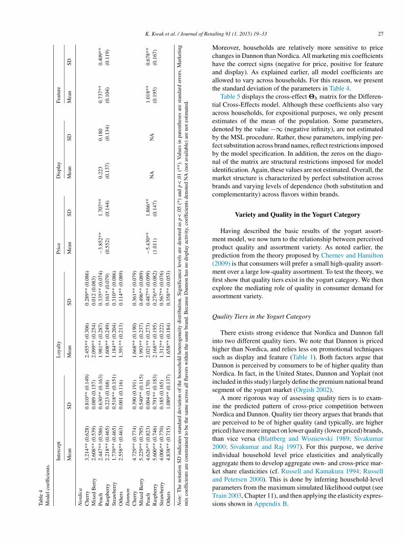

K. Kwak et al. / Journal of RetaTa

ble

4M

odel

coef

ficie

nts.

Inte

rcep

t

Loy

alty

Pric

e

Dis

play

Feat

ure

Mea

n

SD

Mea

n

SD

Mea

n

SD

Mea

n

SD

Mea

n

SD

Nor

dica

Che

rry

3.21

4**

(0.6

28)

0.81

0**

(0.1

49)

2.45

5**

(0.3

06)

0.28

9**

(0.0

86)

−3.8

52**

(0.5

52)

1.70

7**

(0.1

44)

0.22

3(0

.137

)0.

180

(0.1

34)

0.73

7**

(0.1

04)

0.40

9**

(0.1

19)

Mix

ed

Ber

ry

2.60

8**

(0.5

39)

0.08

9

(0.1

57)

2.09

9**

(0.2

54)

0.01

2

(0.0

83)

Peac

h

2.44

7**

(0.5

86)

0.63

0**

(0.1

63)

1.98

1**

(0.2

87)

0.33

5**

(0.0

74)

Ras

pber

ry

2.21

8**

(0.4

65)

0.22

3

(0.1

68)

1.60

8**

(0.2

49)

0.16

1*

(0.0

79)

Stra

wbe

rry

1.73

9**

(0.4

65)

0.51

8**

(0.1

51)

1.18

4**

(0.2

04)

0.31

0**

(0.0

86)

Oth

ers

2.55

8**

(0.4

63)

0.00

1

(0.1

16)

1.39

1**

(0.2

13)

0.11

4**

(0.0

89)

Dan

non

Che

rry

4.72

9**

(0.7

74)

0.39

0

(0.1

91)

1.66

8**

(0.1

90)

0.36

1**

(0.0

79)

−5.4

30**

(1.0

11)

1.86

6**

(0.1

47)

NA

NA

1.01

8**

(0.1

95)

0.67

8**

(0.1

67)

Mix

ed

Ber

ry5.

229*

*

(0.7

95)

0.54

0**

(0.1

15)

1.99

3**

(0.2

37)

0.49

6**

(0.0

89)

Peac

h

4.62

6**

(0.8

23)

0.00

4

(0.1

70)

2.02

1**

(0.2

73)

0.48

7**

(0.0

99)

Ras

pber

ry

5.60

0**

(0.7

46)

0.79

1**

(0.1

83)

2.16

8**

(0.1

95)

0.27

6**

(0.0

82)

Stra

wbe

rry

4.00

6**

(0.7

70)

0.18

5

(0.1

65)

1.31

2**

(0.2

22)

0.56

7**

(0.0

76)

Oth

ers

4.83

8**

(0.7

15)

1.08

9**

(0.1

37)

1.65

8**

(0.1

84)

0.35

8**

(0.0

53)

Not

e:

The

nota

tion

SD

indi

cate

s

stan

dard

devi

atio

n

of

the

hous

ehol

d

hete

roge

neity

dist

ribu

tion.

Sign

ifica

nce

leve

ls

are

deno

ted

as

p

<

.05

(*)

and

p <

.01

(**)

. Val

ues

in

pare

nthe

ses

are

stan

dard

erro

rs. M

arke

ting

mix

coef

ficie

nts

are

cons

trai

ned

to

be

the

sam

e

acro

ss

all fl

avor

s

with

in

the

sam

e

bran

d.

Bec

ause

Dan

non

has

no

disp

lay

activ

ity, c

oeffi

cien

ts

deno

ted

NA

(not

avai

labl

e)

are

not e

stim

ated

.

Mchaat

taedbfbnimbc

mpp(mfiea

Q

ihsDNis

iNapt2iakapTs

iling 91 (1, 2015) 19–33 27

oreover, households are relatively more sensitive to pricehanges in Dannon than Nordica. All marketing mix coefficientsave the correct signs (negative for price, positive for featurend display). As explained earlier, all model coefficients arellowed to vary across households. For this reason, we presenthe standard deviation of the parameters in Table 4.

Table 5 displays the cross-effect �h matrix for the Differen-ial Cross-Effects model. Although these coefficients also varycross households, for expositional purposes, we only presentstimates of the mean of the population. Some parameters,enoted by the value −∞ (negative infinity), are not estimatedy the MSL procedure. Rather, these parameters, implying per-ect substitution across brand names, reflect restrictions imposedy the model specification. In addition, the zeros on the diago-al of the matrix are structural restrictions imposed for modeldentification. Again, these values are not estimated. Overall, the

arket structure is characterized by perfect substitution acrossrands and varying levels of dependence (both substitution andomplementarity) across flavors within brands.

Variety and Quality in the Yogurt Category

Having described the basic results of the yogurt assort-ent model, we now turn to the relationship between perceived

roduct quality and assortment variety. As noted earlier, therediction from the theory proposed by Chernev and Hamilton2009) is that consumers will prefer a small high-quality assort-ent over a large low-quality assortment. To test the theory, werst show that quality tiers exist in the yogurt category. We thenxplore the mediating role of quality in consumer demand forssortment variety.

uality Tiers in the Yogurt Category

There exists strong evidence that Nordica and Dannon fallnto two different quality tiers. We note that Dannon is pricedigher than Nordica, and relies less on promotional techniquesuch as display and feature (Table 1). Both factors argue thatannon is perceived by consumers to be of higher quality thanordica. In fact, in the United States, Dannon and Yoplait (not

ncluded in this study) largely define the premium national brandegment of the yogurt market (Orgish 2002).

A more rigorous way of assessing quality tiers is to exam-ne the predicted pattern of cross-price competition betweenordica and Dannon. Quality tier theory argues that brands that

re perceived to be of higher quality (and typically, are higherriced) have more impact on lower quality (lower priced) brands,han vice versa (Blattberg and Wisniewski 1989; Sivakumar000; Sivakumar and Raj 1997). For this purpose, we derivendividual household level price elasticities and analyticallyggregate them to develop aggregate own- and cross-price mar-et share elasticities (cf. Russell and Kamakura 1994; Russell

nd Petersen 2000). This is done by inferring household-levelarameters from the maximum simulated likelihood output (seerain 2003, Chapter 11), and then applying the elasticity expres-ions shown in Appendix B.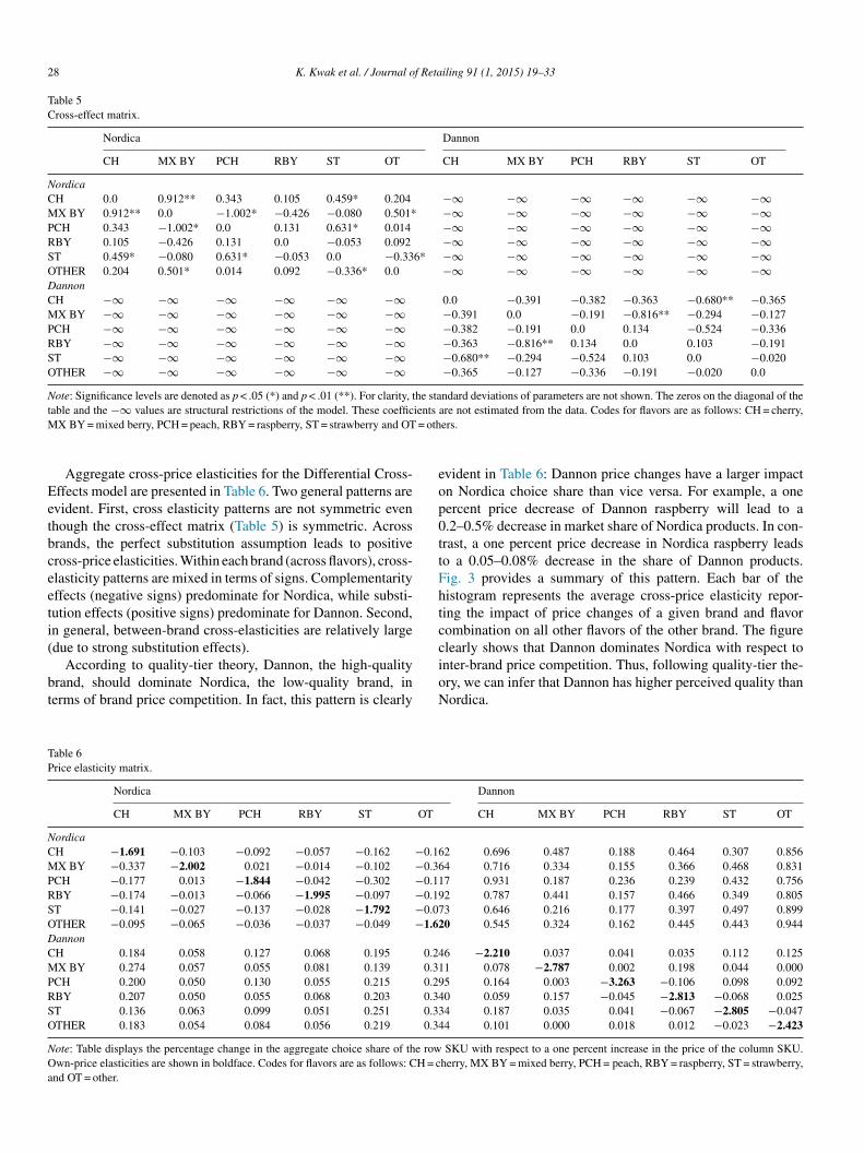

28 K. Kwak et al. / Journal of Retailing 91 (1, 2015) 19–33

Table 5Cross-effect matrix.

Nordica Dannon

CH MX BY PCH RBY ST OT CH MX BY PCH RBY ST OT

NordicaCH 0.0 0.912** 0.343 0.105 0.459* 0.204 −∞ −∞ −∞ −∞ −∞ −∞MX BY 0.912** 0.0 −1.002* −0.426 −0.080 0.501* −∞ −∞ −∞ −∞ −∞ −∞PCH 0.343 −1.002* 0.0 0.131 0.631* 0.014 −∞ −∞ −∞ −∞ −∞ −∞RBY 0.105 −0.426 0.131 0.0 −0.053 0.092 −∞ −∞ −∞ −∞ −∞ −∞ST 0.459* −0.080 0.631* −0.053 0.0 −0.336* −∞ −∞ −∞ −∞ −∞ −∞OTHER 0.204 0.501* 0.014 0.092 −0.336* 0.0 −∞ −∞ −∞ −∞ −∞ −∞DannonCH −∞ −∞ −∞ −∞ −∞ −∞ 0.0 −0.391 −0.382 −0.363 −0.680** −0.365MX BY −∞ −∞ −∞ −∞ −∞ −∞ −0.391 0.0 −0.191 −0.816** −0.294 −0.127PCH −∞ −∞ −∞ −∞ −∞ −∞ −0.382 −0.191 0.0 0.134 −0.524 −0.336RBY −∞ −∞ −∞ −∞ −∞ −∞ −0.363 −0.816** 0.134 0.0 0.103 −0.191ST −∞ −∞ −∞ −∞ −∞ −∞ −0.680** −0.294 −0.524 0.103 0.0 −0.020OTHER −∞ −∞ −∞ −∞ −∞ −∞ −0.365 −0.127 −0.336 −0.191 −0.020 0.0

Note: Significance levels are denoted as p < .05 (*) and p < .01 (**). For clarity, the standard deviations of parameters are not shown. The zeros on the diagonal of thetable and the −∞ values are structural restrictions of the model. These coefficients are not estimated from the data. Codes for flavors are as follows: CH = cherry,M = oth

Eetbceeti(

bt

eop0ttFhtcc

TP

NCMPRSODCMPRSO

NOa

X BY = mixed berry, PCH = peach, RBY = raspberry, ST = strawberry and OT

Aggregate cross-price elasticities for the Differential Cross-ffects model are presented in Table 6. Two general patterns arevident. First, cross elasticity patterns are not symmetric evenhough the cross-effect matrix (Table 5) is symmetric. Acrossrands, the perfect substitution assumption leads to positiveross-price elasticities. Within each brand (across flavors), cross-lasticity patterns are mixed in terms of signs. Complementarityffects (negative signs) predominate for Nordica, while substi-ution effects (positive signs) predominate for Dannon. Second,n general, between-brand cross-elasticities are relatively largedue to strong substitution effects).

According to quality-tier theory, Dannon, the high-qualityrand, should dominate Nordica, the low-quality brand, inerms of brand price competition. In fact, this pattern is clearly

ioN

able 6rice elasticity matrix.

Nordica

CH MX BY PCH RBY ST OT

ordicaH −1.691 −0.103 −0.092 −0.057 −0.162 −0.16X BY −0.337 −2.002 0.021 −0.014 −0.102 −0.36

CH −0.177 0.013 −1.844 −0.042 −0.302 −0.11BY −0.174 −0.013 −0.066 −1.995 −0.097 −0.19T −0.141 −0.027 −0.137 −0.028 −1.792 −0.07THER −0.095 −0.065 −0.036 −0.037 −0.049 −1.62annonH 0.184 0.058 0.127 0.068 0.195 0.24X BY 0.274 0.057 0.055 0.081 0.139 0.31

CH 0.200 0.050 0.130 0.055 0.215 0.29BY 0.207 0.050 0.055 0.068 0.203 0.34T 0.136 0.063 0.099 0.051 0.251 0.33THER 0.183 0.054 0.084 0.056 0.219 0.34

ote: Table displays the percentage change in the aggregate choice share of the rowwn-price elasticities are shown in boldface. Codes for flavors are as follows: CH = c

nd OT = other.

ers.

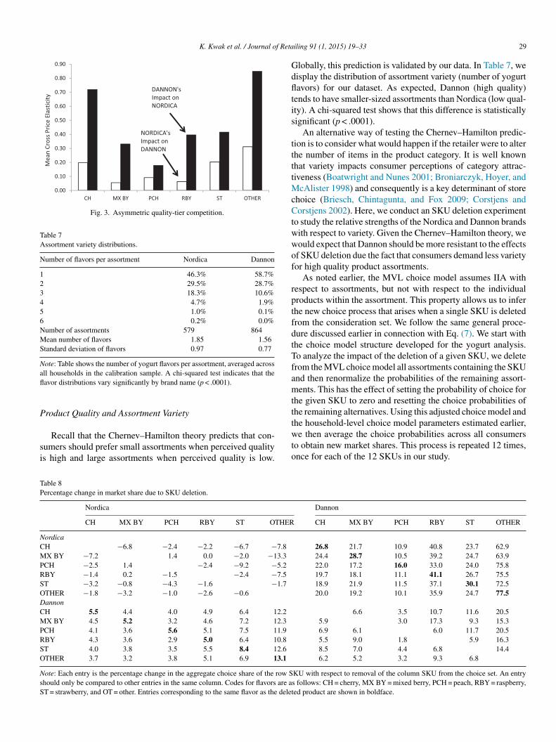
vident in Table 6: Dannon price changes have a larger impactn Nordica choice share than vice versa. For example, a oneercent price decrease of Dannon raspberry will lead to a.2–0.5% decrease in market share of Nordica products. In con-rast, a one percent price decrease in Nordica raspberry leadso a 0.05–0.08% decrease in the share of Dannon products.ig. 3 provides a summary of this pattern. Each bar of theistogram represents the average cross-price elasticity repor-ing the impact of price changes of a given brand and flavorombination on all other flavors of the other brand. The figurelearly shows that Dannon dominates Nordica with respect to

nter-brand price competition. Thus, following quality-tier the-ry, we can infer that Dannon has higher perceived quality thanordica.

Dannon

CH MX BY PCH RBY ST OT

2 0.696 0.487 0.188 0.464 0.307 0.8564 0.716 0.334 0.155 0.366 0.468 0.8317 0.931 0.187 0.236 0.239 0.432 0.7562 0.787 0.441 0.157 0.466 0.349 0.8053 0.646 0.216 0.177 0.397 0.497 0.8990 0.545 0.324 0.162 0.445 0.443 0.944

6 −2.210 0.037 0.041 0.035 0.112 0.1251 0.078 −2.787 0.002 0.198 0.044 0.0005 0.164 0.003 −3.263 −0.106 0.098 0.0920 0.059 0.157 −0.045 −2.813 −0.068 0.0254 0.187 0.035 0.041 −0.067 −2.805 −0.0474 0.101 0.000 0.018 0.012 −0.023 −2.423

SKU with respect to a one percent increase in the price of the column SKU.herry, MX BY = mixed berry, PCH = peach, RBY = raspberry, ST = strawberry,

K. Kwak et al. / Journal of Reta

Fig. 3. Asymmetric quality-tier competition.

Table 7Assortment variety distributions.

Number of flavors per assortment Nordica Dannon

1 46.3% 58.7%2 29.5% 28.7%3 18.3% 10.6%4 4.7% 1.9%5 1.0% 0.1%6 0.2% 0.0%Number of assortments 579 864Mean number of flavors 1.85 1.56Standard deviation of flavors 0.97 0.77

Note: Table shows the number of yogurt flavors per assortment, averaged acrossafl

P

si

Gdfltis

ttttMcCtwwof

rptfdtTfamttt

TP

NCMPRSODCMPRSO

NsS

ll households in the calibration sample. A chi-squared test indicates that theavor distributions vary significantly by brand name (p < .0001).

roduct Quality and Assortment Variety

Recall that the Chernev–Hamilton theory predicts that con-umers should prefer small assortments when perceived qualitys high and large assortments when perceived quality is low.

wto

able 8ercentage change in market share due to SKU deletion.

Nordica

CH MX BY PCH RBY ST OTHER

ordicaH −6.8 −2.4 −2.2 −6.7 −7.8

X BY −7.2 1.4 0.0 −2.0 −13.3

CH −2.5 1.4 −2.4 −9.2 −5.2

BY −1.4 0.2 −1.5 −2.4 −7.5

T −3.2 −0.8 −4.3 −1.6 −1.7

THER −1.8 −3.2 −1.0 −2.6 −0.6

annonH 5.5 4.4 4.0 4.9 6.4 12.2

X BY 4.5 5.2 3.2 4.6 7.2 12.3

CH 4.1 3.6 5.6 5.1 7.5 11.9

BY 4.3 3.6 2.9 5.0 6.4 10.8

T 4.0 3.8 3.5 5.5 8.4 12.6

THER 3.7 3.2 3.8 5.1 6.9 13.1

ote: Each entry is the percentage change in the aggregate choice share of the row Should only be compared to other entries in the same column. Codes for flavors are aT = strawberry, and OT = other. Entries corresponding to the same flavor as the delet

iling 91 (1, 2015) 19–33 29

lobally, this prediction is validated by our data. In Table 7, weisplay the distribution of assortment variety (number of yogurtavors) for our dataset. As expected, Dannon (high quality)

ends to have smaller-sized assortments than Nordica (low qual-ty). A chi-squared test shows that this difference is statisticallyignificant (p < .0001).

An alternative way of testing the Chernev–Hamilton predic-ion is to consider what would happen if the retailer were to alterhe number of items in the product category. It is well knownhat variety impacts consumer perceptions of category attrac-iveness (Boatwright and Nunes 2001; Broniarczyk, Hoyer, and

cAlister 1998) and consequently is a key determinant of storehoice (Briesch, Chintagunta, and Fox 2009; Corstjens andorstjens 2002). Here, we conduct an SKU deletion experiment

o study the relative strengths of the Nordica and Dannon brandsith respect to variety. Given the Chernev–Hamilton theory, weould expect that Dannon should be more resistant to the effectsf SKU deletion due the fact that consumers demand less varietyor high quality product assortments.

As noted earlier, the MVL choice model assumes IIA withespect to assortments, but not with respect to the individualroducts within the assortment. This property allows us to inferhe new choice process that arises when a single SKU is deletedrom the consideration set. We follow the same general proce-ure discussed earlier in connection with Eq. (7). We start withhe choice model structure developed for the yogurt analysis.o analyze the impact of the deletion of a given SKU, we deleterom the MVL choice model all assortments containing the SKUnd then renormalize the probabilities of the remaining assort-ents. This has the effect of setting the probability of choice for

he given SKU to zero and resetting the choice probabilities ofhe remaining alternatives. Using this adjusted choice model andhe household-level choice model parameters estimated earlier,

e then average the choice probabilities across all consumers

o obtain new market shares. This process is repeated 12 times,nce for each of the 12 SKUs in our study.

Dannon

CH MX BY PCH RBY ST OTHER

26.8 21.7 10.9 40.8 23.7 62.924.4 28.7 10.5 39.2 24.7 63.922.0 17.2 16.0 33.0 24.0 75.819.7 18.1 11.1 41.1 26.7 75.518.9 21.9 11.5 37.1 30.1 72.520.0 19.2 10.1 35.9 24.7 77.5

6.6 3.5 10.7 11.6 20.55.9 3.0 17.3 9.3 15.36.9 6.1 6.0 11.7 20.55.5 9.0 1.8 5.9 16.38.5 7.0 4.4 6.8 14.46.2 5.2 3.2 9.3 6.8

KU with respect to removal of the column SKU from the choice set. An entrys follows: CH = cherry, MX BY = mixed berry, PCH = peach, RBY = raspberry,ed product are shown in boldface.

3 f Reta

bsOeTbdo

SwocNsbDD

S

cqtceCoq

vcstspv

S

oiamiothvvs

iv

pn(plupcficptam

M

fhufmb2rdptccdi

L

pc(sgoicperB2

0 K. Kwak et al. / Journal o

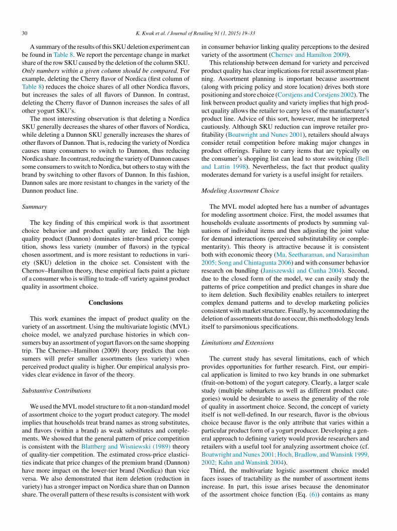
A summary of the results of this SKU deletion experiment cane found in Table 8. We report the percentage change in markethare of the row SKU caused by the deletion of the column SKU.nly numbers within a given column should be compared. For

xample, deleting the Cherry flavor of Nordica (first column ofable 8) reduces the choice shares of all other Nordica flavors,ut increases the sales of all flavors of Dannon. In contrast,eleting the Cherry flavor of Dannon increases the sales of allther yogurt SKU’s.

The most interesting observation is that deleting a NordicaKU generally decreases the shares of other flavors of Nordica,hile deleting a Dannon SKU generally increases the shares ofther flavors of Dannon. That is, reducing the variety of Nordicaauses many consumers to switch to Dannon, thus reducingordica share. In contrast, reducing the variety of Dannon causes

ome consumers to switch to Nordica, but others to stay with therand by switching to other flavors of Dannon. In this fashion,annon sales are more resistant to changes in the variety of theannon product line.

ummary

The key finding of this empirical work is that assortmenthoice behavior and product quality are linked. The highuality product (Dannon) dominates inter-brand price compe-ition, shows less variety (number of flavors) in the typicalhosen assortment, and is more resistant to reductions in vari-ty (SKU) deletion in the choice set. Consistent with thehernov–Hamilton theory, these empirical facts paint a picturef a consumer who is willing to trade-off variety against productuality in assortment choice.

Conclusions

This work examines the impact of product quality on theariety of an assortment. Using the multivariate logistic (MVL)hoice model, we analyzed purchase histories in which con-umers buy an assortment of yogurt flavors on the same shoppingrip. The Chernev–Hamilton (2009) theory predicts that con-umers will prefer smaller assortments (less variety) whenerceived product quality is higher. Our empirical analysis pro-ides clear evidence in favor of the theory.

ubstantive Contributions

We used the MVL model structure to fit a non-standard modelf assortment choice to the yogurt product category. The modelmplies that households treat brand names as strong substitutes,nd flavors (within a brand) as weak substitutes and comple-ents. We showed that the general pattern of price competition

s consistent with the Blattberg and Wisniewski (1989) theoryf quality-tier competition. The estimated cross-price elastici-ies indicate that price changes of the premium brand (Dannon)

ave more impact on the lower-tier brand (Nordica) than viceersa. We also demonstrated that item deletion (reduction inariety) has a stronger impact on Nordica share than on Dannonhare. The overall pattern of these results is consistent with work

fio

iling 91 (1, 2015) 19–33

n consumer behavior linking quality perceptions to the desiredariety of the assortment (Chernev and Hamilton 2009).

This relationship between demand for variety and perceivedroduct quality has clear implications for retail assortment plan-ing. Assortment planning is important because assortmentalong with pricing policy and store location) drives both storeositioning and store choice (Corstjens and Corstjens 2002). Theink between product quality and variety implies that high prod-ct quality allows the retailer to carry less of the manufacturer’sroduct line. Advice of this sort, however, must be interpretedautiously. Although SKU reduction can improve retailer pro-tability (Boatwright and Nunes 2001), retailers should alwaysonsider retail competition before making major changes inroduct offerings. Failure to carry items that are typically onhe consumer’s shopping list can lead to store switching (Bellnd Lattin 1998). Nevertheless, the fact that product qualityoderates demand for variety is a useful insight for retailers.

odeling Assortment Choice

The MVL model adopted here has a number of advantagesor modeling assortment choice. First, the model assumes thatouseholds evaluate assortments of products by summing val-ations of individual items and then adjusting the joint valueor demand interactions (perceived substitutability or comple-entarity). This theory is attractive because it is consistent

oth with economic theory (Ma, Seetharaman, and Narasimhan005; Song and Chintagunta 2006) and with consumer behavioresearch on bundling (Janiszewski and Cunha 2004). Second,ue to the closed form of the model, we can easily study theatterns of price competition and predict changes in share dueo item deletion. Such flexibility enables retailers to interpretomplex demand patterns and to develop marketing policiesonsistent with market structure. Finally, by accommodating theeletion of assortments that do not occur, this methodology lendstself to parsimonious specifications.

imitations and Extensions

The current study has several limitations, each of whichrovides opportunities for further research. First, our empiri-al application is limited to two key brands in one submarketfruit-on-bottom) of the yogurt category. Clearly, a larger scaletudy (multiple submarkets as well as different product cate-ories) would be desirable to assess the generality of the rolef quality in assortment choice. Second, the concept of varietytself is not well-defined. In our research, flavor is the obvioushoice because flavor is the only attribute that varies within aarticular product form of a yogurt producer. Developing a gen-ral approach to defining variety would provide researchers andetailers with a useful tool for analyzing assortment choice (cf.oatwright and Nunes 2001; Hoch, Bradlow, and Wansink 1999,002; Kahn and Wansink 2004).

Third, the multivariate logistic assortment choice modelaces issues of tractability as the number of assortment itemsncrease. In part, this issue arises because the denominatorf the assortment choice function (Eq. (6)) contains as many

f Reta

tdtm(ewaya

gomedtdipf

BtiP

t

., zJ

. ., zJ

IP

a

ltswsiittv

btTaiTtm

toyet

dh

E

E

pci

w

P

Pr(j, k)ht

=∑

b containg item j and k

exp(

�′htz

bht + 1

2

{zbht ′�hzb

ht

})∑

b∗ exp(

�′htz

b∗ht + 1

2

{zb∗ht ′�hzb∗

ht

})(B4)

K. Kwak et al. / Journal o

erms as possible assortments. In this research, we avoided theimensionality problem by using structural assumptions to limithe number of possible assortments. Currently, simulation esti-

ation technologies that approximate the denominator of Eq.6) exist, but are confined to models without parameter het-rogeneity (see, e.g., Wu and Huffer 1997). However, recentork by Kamakura and Kwak (2012) involving sampling of

lternatives (Ben-Akiva and Lerman 1985) and latent class anal-sis (Kamakura and Russell 1989) shows promise in developing

practical method of model calibration.In addition, the number of cross-effect parameters increases

eometrically with the number of items in the study. The obvi-us solution here is to constrain the pattern of the cross-effectatrix to reduce the number of parameters in the model. For

xample, cross-effect parameters can be projected into a reducedimensional space (Kamakura and Schimmel 2013). Alterna-ively, the cross-effect pattern can be made to correspond to theistances on a psychometric map representing similarity amongtems (Moon and Russell 2008). Successfully addressing theseroblems would allow retailers to use the model to study choiceor large numbers of assortments.

Appendix A. Derivation of Assortment Model

Let z = (z1, z2, . . ., zJ ) be any assortment of item choices.rook’s Lemma, cited in Besag (1974), states that the joint dis-

ribution of the random variable zj, namely Pr(z1, z2, . . ., zJ ),s proportional to a series of ratios through a certain constantr(z10, z20, . . ., zJ0) where zj0 is an arbitrary reference value of

he random variable zj. Specifically, Brook’s Lemmas states that

Pr(z1, z2, . . ., zJ )

Pr(z10, z20, . . ., zJ0)= Pr(z1|z2, z3, . . ., zJ )

Pr(z10|z2, z3, . . ., zJ )

Pr(z2|z10, z3, . .

Pr(z20|z10, z3, .

n this research, we define the joint distributionr(z1, z2, . . ., zJ ) to be the probability of choosing anssortment of products.

We derive an assortment choice model in Eq. (6) in the fol-owing way. First, we assume (without loss of generality) thathe reference values zj0 = 0 so that the proportionality con-tant Pr(z10, z20, . . ., zJ0) is equal to Pr(0, 0, . . ., 0). Second,e assume that all the conditional probabilities on the right hand

ide of (A1) have the form of the binary logit expressions foundn Eq. (5). Third, we assume that all elements of the �h matrixn Eq. (3) are symmetric. This last assumption essentially meanshat the probability of observing an assortment depends only onhe contents of the assortment – not upon the order in which thearious products in the assortment are purchased.

The assortment choice probability given in Eq. (6) is obtainedy inserting these assumptions into (A1) and using the fact thathe sum of the probabilities over all assortments must add to one.he symmetry of �h ensures that the assortment model gener-ted by (A1) always has the same form, regardless of the order

n which the SKU’s are placed in the z = (z1, z2, . . ., zJ ) vector.he model implicitly assumes that any assortment – including

he null assortment with probability equal to Pr(0, 0, . . ., 0) –ay be observed. However, the analyst can restrict the model

w

F

b

iling 91 (1, 2015) 19–33 31

)

)· · · Pr(zJ |z10, z20, . . ., zJ−1,0)

Pr(zJ0|z10, z20, . . ., zJ−1,0)(A1)

o a subset of assortments by restricting the possible valuesf z and then renormalizing the resulting model. In the anal-sis of the yogurt data, we followed this procedure in order toxclude assortments that cannot occur (e.g., assortments con-aining items with different brand names).

Appendix B. Derivation of Price Elasticities

We first derive household-level price elasticities. Let j and kenote two different SKU’s. At specific time point t for house-old h, elasticities are computed as

(j, j)ht = ∂[ln Pr(j)ht]

∂[ln PRICE(j)ht]= ∂Pr(j)ht

∂PRICE(j)ht

PRICE(j)ht

Pr(j)ht

(B1)

(jc, kc∗)ht = ∂[ln Pr(jc)ht

]∂[ln PRICE(kc∗)ht

]= ∂Pr(jc)ht

∂PRICE(kc∗)ht

PRICE(kc∗)ht

Pr(jc)ht

(B2)

Given the form of the model, we can write probability ofurchasing item j by enumerating all probabilities of assortmentsontaining item j. We can also define the probability of choosingtem j and k in one assortment in the same way. These can be

ritten as

r(j)ht =∑

b containg item j

exp(

�′htz

bht + 1

2

{zbht ′�hzb

ht

})∑

b∗ exp(

�′htz

b∗ht + 1

2

{zb∗ht ′�hzb∗

ht

})(B3)

here πphjt = α

phj + β

p1,hPRICEhpt + β

p2,hDISPhpt + β

p3,h

EAThpt + βp4,hLOYhj and marketing mix parameters are

rand specific, not item specific.

3 f Reta

t

has b

rand

/= k

Ai

/= q

/= k

wmitS

an(tKhi

ICE

Epk

h

]}]

A

B

B

B

B

B

B

B

B

B

B

C

2 K. Kwak et al. / Journal o

Using simple algebra, we can derive the following deriva-ives:

∂Pr(jp)ht

∂PRICE(jp)ht

= βp1,hPr(jp)

ht(1 − Pr(jp)

ht) if j

∂Pr(jp)ht

∂PRICE(kq)ht

= −βq1,hPr(jp)

htPr(kq)

htif b

∂Pr(jp)ht

∂PRICE(kp)ht

= βp1,h{Pr(jp, kp)

ht− Pr(jp)

htPr(kp)

ht} if j

pplying elasticity definitions in (B1) and (B2), the correspond-ng household-level elasticities are computed as:

E(jp, jp)ht

= βpprice{1 − Pr(jp)

ht}PRICE

phjt

E(jp, kq)ht

= −βqpricePr(kq)

htPRICE

qhkt if p

E(jp, kp)ht

= βppricePr(kp)

ht{S(jp, kp)

ht− 1}PRICE

phkt if j

here S(j, k)ht = Pr(j, k)ht/Pr(j)htPr(k)ht . When there areore than two items in a category, cross-elasticity between two

tems in same category is not solely determined by cross-effecterms but by S(j, k). Notice that S(j, k) > 0 for complements,(j, k) < 0 for substitutes, and S(j, k) = 0 for independence.

To compute aggregate elasticities, we first define the over-ll choice shares as MSj = ∑

h

∑tPr(j)ht/NT where NT (the

umber households (N) times average number of shopping tripsT) per household) is the number of total observations in a par-icular data set. Following procedures outlined in Russell andamakura (1994), we differentiate this expression and use theousehold level derivatives in (B5) to infer market share elastic-ties. This process yields the expressions

ηjj = %�MS(jp)

%PRICEpj

=[{∑

hβphPr(jp)

h[1 − Pr(jp)

h]}

/N

MS(jp)

]PR

ηp,qjk = %�MS(jp)

%PRICEqk

= −[{∑

hβqhPr(jp)

hPr(kq)

h

}/N

MS(jp)

]PRIC

ηpjk = %�MS(jp)

%PRICEpk

=[{∑

hβph

[Pr(jp, kp)

h− Pr(jp)

hPr(kp)

MS(jp)

References

nselin, Luc (2002), “Under the Hood: Issues in Specification and Interpretationof Spatial Regression Models,” Agricultural Economics, 27 (November),247–67.

ell, David and James Lattin (1998), “Shopping Behavior and Consumer Pref-erence for Store Price Format: Why Large Basket Shoppers Prefer EDLP,”Marketing Science, 17 (1), 66–88.

en-Akiva, Moshe and Steven R. Lerman (1985), Discrete Choice Analysis:Theory and Application to Travel Demand, Cambridge, MA: MIT Press.

esag, Julian (1974), “Spatial Interaction and the Statistical Analysis of LatticeSystems,” Journal of the Royal Statistical Society B, 36, 192–236.

lattberg, Robert C. and Kenneth J. Wisniewski (1989), “Price-Induced Patterns

of Competition,” Marketing Science, 8 (4), 291–309.

oatwright, Peter and Joseph C. Nunes (2001), “Reducing Assortment: AnAttribute-Based Approach,” Journal of Marketing, 65 (July), 50–63.

otti, Simona and Ann L. McGill (2006), “When Choosing is Not Deciding: TheEffect of Perceived Responsibility on Satisfaction,” Journal of ConsumerResearch, 33 (September), 211–9.

C

C

iling 91 (1, 2015) 19–33

rand p

p /= q

for different brands

(B5)

have the same brand

(B6)

pj

for brands p /= q

PRICEpk j /= k for same brand

(B7)

oztug, Yasemin and Lutz Hildebrandt (2008), “Modeling Joint PurchasesWith a Multivariate MNL Approach,” Schmalenbach Business Review, 60(October), 400–22.

riesch, Richard A., Pradeep K. Chintagunta and Edward J. Fox (2009), “HowDoes Assortment Affect Grocery Store Choice,” Journal of MarketingResearch, 66 (April), 176–89.

roniarczyk, Susan M., Wayne D. Hoyer and Leigh McAlister (1998), “Con-sumers’ Perceptions of the Assortment Offered in a Grocery Category:The Impact of Item Reduction,” Journal of Marketing Research, 35 (May),166–76.

roniarczyk, Susan (2008), “Product Assortment,” in Handbook of ConsumerPsychology New York, NY: Lawrence Erlbaum Associates.755–79.

hernev, Alexander (2011), “Product Assortment and Consumer Choice: AnInterdisciplinary Review,” Foundations and Trends in Marketing, 6 (1), 1–61.

hernev, Alexander and Ryan Hamilton (2009), “Assortment Size and Option

Attractiveness in Consumer Choice Among Retailers,” Journal of MarketingResearch, 44 (June), 410–20.

hung, J. and Vithala R. Rao (2003), “A General Choice Model for Bundleswith Multiple-Category Products: Application to Market Segmentation and

f Reta

C

C

C

F

G

G

G

H

H

H

H

J

K

K

K

K

K

K

K

K

K

K

K

L

L

M

M

M

N

O

R

R

R

S

S

S

S

S

S

T

V

W

W

K. Kwak et al. / Journal o

Optimal Pricing for Bundles,” Journal of Marketing Research, 40 (May),115–30.

orstjens, Judith and Marcel Corstjens (2002), Store Wars: The Battle forMindspace and Shelfspace, New York: John Wiley and Sons.

ox, David R. (1972), “The Analysis of Multivariate Binary Data,” AppliedStatistics (Journal of the Royal Statistical Society Series C, 21 (2),113–20.

ressie, Noel A.C. (1993), Statistics for Spatial Data, New York: John Wileyand Sons.

arquhar, Peter H. and Vithala R. Rao (1976), “A Balance Model for EvaluatingSubsets of Multiattributed Items,” Management Science, 22 (5), 528–39.

entzkow, Matthew (2007), “Valuing New Goods in a Model With Comple-mentarity: Online Newspapers,” The American Economic Review, 97 (3),713–44.

ourville, John T. and Dilip Soman (2005), “Overchoice and AssortmentType: When and Why Variety Backfires,” Marketing Science, 24 (Summer),382–95.

reen, Paul H., Wind Yoram and A.K. Jain (1972), “Preference Measurementof Item Collections,” Journal of Marketing Research, 9 (November), 371–7.

arlam, Bari A. and Leonard M. Lodish (1995), “Modeling Consumers’Choices of Multiple Items,” Journal of Marketing Research, 32 (November),404–18.

och, Stephen J., Eric T. Bradlow and Brian Wansink (1999), “The Variety ofan Assortment,” Marketing Science, 18 (4), 527–46.

, and(2002), “Rejoinder to “The Variety of An Assortment: An Extension to theAttribute-Based Approach”,” Marketing Science, 21 (Summer), 342–6.

oyer, Wayne D. (1984), “An Examination of Decision Making for a CommonRepeat-Purchase Product,” Journal of Consumer Research, 11, 822–9.

uber, Joel and Kenneth Train (2001), “On the Similarity of Classical andBayesian Estimates of Individual Mean Parthworths,” Marketing Letters,12 (August), 259–69.

aniszewski, Chris and Marcus Cunha Jr. (2004), “The Influence of Price Dis-count Framing on the Evaluation of a Product Bundle,” Journal of ConsumerResearch, 30 (March), 534–46.

ahn, Barbara E. (1995), “Consumer Variety-Seeking Among Goods and Ser-vices,” Journal of Retailing & Consumer Services, 2 (July), 139–48.

ahn, Barbara E. and Donald R. Lehmann (1991), “Modeling Choice AmongAssortments,” Journal of Retailing, 67 (3), 274–99.

ahn, Barbara E. and Brian Wansink (2004), “The Influence of AssortmentStructure on Perceived Variety and Consumption Quantities,” Journal ofConsumer Research, 30 (March), 519–33.

ahn, Barbara E., William L. Moore and Rashi Glazer (1987), “Experiments inConstrained Choice,” Journal of Consumer Research, 14 (June), 96–113.

ahneman, Daniel and Jackie Snell (1990), “Predicting Utility,” in Insights inDecision Making: A Tribute to Hillel J. Einhorn, Hogarth Robin M. ed.Chicago: University of Chicago Press, 295–310.

ahneman, Daniel and Jackie S. Snell (1992), “Predicting a Changing Taste:Do People Know What They Will Like?,” Journal of Behavioral DecisionMaking, 5 (3), 187–200.

amakura, Wagner A. and Gary J. Russell (1989), “A Probabilistic ChoiceModel for Market Segmentation and Elasticity Structure,” Journal of Mar-keting Research, 26 (November), 379–90.

amakura, Wagner A. and Kyuseop Kwak (2012), Menu-Choice Modeling,working paper. Rice University.

amakura, Wagner A. and Carl Schimmel (2013), “Uncovering AudiencePreferences for Concert Features From Single-Ticket Sales With a Factor-Analytic Random-Coefficients Model,” International Journal of Researchin Marketing, 30 (2), 129–42.

Y

iling 91 (1, 2015) 19–33 33

im, Jaehwan, Greg M. Allenby and Peter E. Rossi (2002), “Modeling Con-sumer Demand for Variety,” Marketing Science, 21 (Summer), 229–50.

uksov, Dmitri and J. Miguel Villas-Boas (2010), “When More AlternativesLead to Less Choice,” Marketing Science, 29 (May–June), 507–24.

ee, Lung-Fei (1995), “Asymptotic Bias in Simulated Maximum LikelihoodEstimates of Discrete Choice Models,” Econometric Theory, 11, 437–83.

uce, Mary Frances (1992), “Buying More Than We Can Use: Factors Influ-encing Forecasts of Consumption Quantity,” In Advances in ConsumerResearch, Vol. 19, Sherry John F. Jr. and Sternthal Brian eds. , 584–8.

a, Yu, P.B. (Seethu) Seetharaman and Chakravarthi Narasimhan (2005),Empirical Analysis of Competitive Pricing Strategies with ComplementaryProduct Lines, Working Paper. University of Alberta.

arkman, Art. B. and D. Gentner (1993), “Structural Alignment During Simi-larity Comparisons,” Cognitive Psychology, 25 (October), 431–67.

oon, Sangkil and Gary J. Russell (2008), “Predicting Product Purchase FromInferred Customer Similarity: An Autologistic Model Approach,” Manage-ment Science, 54 (January), 71–82.

iraj, Rakesh, V. Padmanabhan and P.B. Seetharaman (2008), “A Cross-Category Model of Households’ Incidence and Quantity Decisions,”Marketing Science, 27 (March–April), 225–35.

rgish, Stephen (2002), Market Report on the Refrigerated Yogurt Market inthe USA, Houston: Swiss Business Hub, United States of America.

ao, Vithala R. (2004), “Bundles of Multi-attributed Items: ModelingPerceptions, Preferences and Choice,” in Cross-Functional Innovation Man-agement: Perspectives From Different Disciplines Working Paper, AlbersSonke ed. New York: Gabler Publishers, 176–90.

ussell, Gary J. and Ann Petersen (2000), “Analysis of Cross Category Depend-ence in Market Basket Selection,” Journal of Retailing, 76 (3), 367–92.

ussell, Gary J. and Wagner A. Kamakura (1994), “Understanding Brand PriceCompetition with Micro and Macro Scanner Data,” Journal of MarketingResearch, 31 (May), 289–303.

hin, Jiwoong and Dan Ariely (2004), “Keeping Doors Open: The Effect ofUnavailability on Incentives to Keep Options Viable,” Management Science,50 (May), 575–86.

hugan, Steven (1980), “The Cost of Thinking,” Journal of Consumer Research,7 (September), 99–111.

imonson, Itamar (1990), “The Effect of Purchase Quantity and Timing on Vari-ety Seeking Behavior,” Journal of Marketing Research, 27 (May), 150–62.

ivakumar, K. (2000), “Price Tier Competition: An Integrative Review,” PricingStrategy and Practice, 9 (5), 276–90.

ivakumar, K. and S.P. Raj (1997), “Quality Tier Competition: How PriceChange Influences Brand Choice and Category Choice,” Journal of Mar-keting, 61 (July), 71–84.

ong, Inseong and Pradeep K. Chintagunta (2006), “Measuring Cross-CategoryPrice Effects with Aggregate Store Data,” Management Science, 52(October), 1594–609.

rain, Kenneth (2003), Discrete Choice Models With Simulation, Cambridge:Cambridge University Press.

an Herpen, Erica and Rik Pieters (2007), “Anticipated Identification Costs:Improving Assortment Evaluation by Diagnostic Attributes,” InternationalJournal of Research in Marketing, 24 (March), 77–88.

alsh, John W. (1995), “Flexibility in Consumer Purchasing for UncertainFuture Tastes,” Marketing Science, 14 (2), 148–65.

u, Hulin and Fred W. Huffer (1997), “Modeling the Distribution of PlantSpecies Using the Autologistic Regression Model,” Environmental and Eco-

logical Statistics, 4, 49–64.

ang, Sha, Yi Zhao, Tulin Erdem and Ying Zhao (2010), “Modeling the Intra-Household Behavioral Interaction,” Journal of Marketing Research, 47(June), 470–84.