An analysis of amenity-led rural economic *development in

Graduate Theses, Dissertations, and Problem Reports

2009

An analysis of amenity-led rural economic *development in An analysis of amenity-led rural economic *development in

northeast region: A spatial simultaneous equations approach northeast region: A spatial simultaneous equations approach

Mulugeta Saare Kahsai West Virginia University

Follow this and additional works at: https://researchrepository.wvu.edu/etd

Recommended Citation Recommended Citation Kahsai, Mulugeta Saare, "An analysis of amenity-led rural economic *development in northeast region: A spatial simultaneous equations approach" (2009). Graduate Theses, Dissertations, and Problem Reports. 2925. https://researchrepository.wvu.edu/etd/2925

This Dissertation is protected by copyright and/or related rights. It has been brought to you by the The Research Repository @ WVU with permission from the rights-holder(s). You are free to use this Dissertation in any way that is permitted by the copyright and related rights legislation that applies to your use. For other uses you must obtain permission from the rights-holder(s) directly, unless additional rights are indicated by a Creative Commons license in the record and/ or on the work itself. This Dissertation has been accepted for inclusion in WVU Graduate Theses, Dissertations, and Problem Reports collection by an authorized administrator of The Research Repository @ WVU. For more information, please contact [email protected].

https://researchrepository.wvu.edu/

https://researchrepository.wvu.edu/

https://researchrepository.wvu.edu/etd

https://researchrepository.wvu.edu/etd?utm_source=researchrepository.wvu.edu%2Fetd%2F2925&utm_medium=PDF&utm_campaign=PDFCoverPages

https://researchrepository.wvu.edu/etd/2925?utm_source=researchrepository.wvu.edu%2Fetd%2F2925&utm_medium=PDF&utm_campaign=PDFCoverPages

mailto:[email protected]

An Analysis of Amenity-Led Rural Economic Development in Northeast Region:

A Spatial Simultaneous Equations Approach

Mulugeta Saare Kahsai

Dissertation submitted to the Davis College of Agriculture, Forestry, and Consumer Sciences

at West Virginia University in partial fulfillment of the requirements

for the degree of

Doctor of Philosophy in

Natural Resource Economics

Dr. Tesfa Gebremedhin, Committee Chairperson

Dr. Peter V. Schaeffer, Co-chair

Dr. Tim T. Phipps

Dr. Dale Colyer

Dr. Stratford Douglas

Agricultural and Resource Economics Program

Division of Resource Management

Morgantown, West Virginia

2009

Keywords: Natural and built amenities, regional economic growth, spatial Durbin model

Copyright 2009 Mulugeta Saare Kahsai

ABSTRACT

An Analysis of Amenity-Led Rural Economic Development in Northeast Region:

A Spatial Simultaneous Equations approach

Mulugeta Saare Kahsai

In a matter of just a few decades, the economic landscape of rural America has changed in fundamental ways. Industries once considered the backbone of rural economies have been transformed by globalization and marketing. Others, such as tourism and amenity-based economies or the service sector, have emerged to replace the traditional natural resource and manufacturing-based economies. These changes have invigorated some areas, and forever altered others. Consequently, Interest in an amenity focused development strategy has exploded as policymakers and community leaders realize that most of the jobs lost in recent decades will not return. Instead, these leaders are looking inside their communities for new sources of economic growth.

In an effort to analyze the role of natural and recreational amenities in rural economic growth, this study develops a simultaneous-equation system under the assumptions of profit maximization of firms and utility maximization of households as well as the neoclassical assumption of equilibrium growth in a partial lag-adjustment growth-equilibrium framework. Past studies assume that amenities have a direct and independent effect on economic growth, but in reality the availability of high amenity levels alone can only create the opportunity for economic growth. But to be an effective development tool it should be coupled with factors that can exploit its existence, encourage its use, and give it a comparative advantage.

This research extends existing studies in this area by incorporating interaction terms that account for the combined impact of amenities with proximity to metropolitan areas and accessibility (Interstate highway density). Furthermore, the study contributes to the amenity and regional growth literature by estimating a simultaneous spatial Durbin model using the two stages least square method. Historical and cultural amenities and water based recreational amenities are found to play a positive role in shaping the growth of population in the northeast region of the US. The role of natural amenities, land and winter based amenities is found to be negative or insignificant. One of the important findings of the study is the positive role of surrounding counties historical and cultural amenities in the growth of population and employment densities. Overall there is no evidence of a consistent and strong relationship and the results can be termed as mixed and inconclusive.

iii

Dedication

I would like to dedicate this work to the life and memory of my late father

Saare Kahsai, my mother Ghenet Fessehazion, my late brother Alem

Saare, and my wife Yodit Asser. I am who I am because of you. You are

my true inspiration.

iv

Acknowledgments This dissertation would have been an impossible task without the support and guidance of my committee members. I would like to express my sincere thanks to all my committee members. I was very fortunate to have a Dr. Tesfa G. Gebremedhin as a chair and Dr. Peter V. Schaeffer as co-chair of my committee. I would first like to thank them for giving me enough freedom to develop my research while not allowing me to stray too far from the path. They supported and guided me to conduct a meaningful research and without their assistance I would not have been able to conduct my research in timely manner. Both professionally and personally, I have enjoyed my association with them. I am grateful to my committee member Dr. Dale Colyer for his comments, suggestions, insights, and for contributing his time generously to edit my manuscript. I wish to thank the other members of my committee, Dr. Tim Phipps, Dr. Stratford Douglas, and the associate dean of Davis College of Agriculture, Forestry, and Consumer Science Dr. Denny Smith for their critical comments, review of the manuscript, and helpful insights. I am indebted to the Division of Resource Management, Davis College of Agriculture, Forestry, and Consumer Sciences, for providing me research assistantship for my first two and half years of my PhD studies. I am thankful to the faculty, staff, and graduate students of the Division of Resource Management. My deepest appreciations also to the Regional Research Institute (RRI) at West Virginia University, its Director Dr. Randall Jackson for the research assistantship for my last year of my study. This dissertation benefited greatly from previous studies done in the Division of Resource Management. In this regard, I am grateful to Dr. Gebremeskel H. Gebremariam and Dr. Yohannes G. Hailu for freely sharing their expertise and knowledge. So many other people have helped me that it is impossible to thank them individually. However I must express my appreciation of the special assistance given to me by Lisa A. Lewis, Melanie Jimmie, Ellen Hartley-Smith, Mary Lou Myer, Ahadu Tecle, and Adiam Tsegai. I wish to express my deepest thanks to my wife, Yodit Asser. Her patience, support, and

encouragement was the source of my strength to finish this dissertation. Finally, the list

of acknowledgments would be incomplete if I did not acknowledge the role of my family

and friends all over the world. I am very blessed to be surrounded by a very special and

caring family and friends who were always there for me. My special thanks to the family

of Saare Kahsai, family of Fessehazion Haile, family of Asser Andemariam, family of Dr.

Tesfa G. Gebremedhin, and family of Amanuel Tesfahunie. Their constant and unfailing

love, financial, and moral support in my pursuit of graduate education, gave me the

energy and motive to stay strong and successful complete this dissertation. I couldn’t

have done it without their support.

v

Table of Contents ABSTRACT ...................................................................................................................................................... ii

Dedication .................................................................................................................................................... iii

Acknowledgments ........................................................................................................................................ iv

Table of Contents .......................................................................................................................................... v

List of Tables ............................................................................................................................................... vii

List of Figures ............................................................................................................................................. viii

CHAPTER 1: INTRODUCTION .................................................................................................................... 1

1.1. Introduction and Problem Statement ................................................................................................ 1

1.2. Overview of the Study Area ............................................................................................................... 7

1.3. Objective of the Study ..................................................................................................................... 12

1.4. Hypotheses ...................................................................................................................................... 12

1.5. Methodology .................................................................................................................................... 14

1.6. Organization of the Study ................................................................................................................ 15

CHAPTER 2: LITERATURE REVIEW ......................................................................................................... 16

2.1. Amenities and Economic Development ........................................................................................... 16

2.2. Measuring Amenity Attributes ........................................................................................................ 18

2.3. Review of Factors Associated With Amenity and Rural Development ............................................ 21

2.4. Methodological Issues ..................................................................................................................... 26

2.5. Summary and Shortcomings of Past Studies ................................................................................... 30

CHAPTER 3: THEORETICAL MODELS OF AMENITIES AND REGIONAL DEVELOPMENT ................. 32

3.1. Household and Firm Location .......................................................................................................... 32

3.1.1. The Household’s Location Decision .......................................................................................... 33

3.1.2. The Firm’s Location Decision .................................................................................................... 34

3.1.3. Interactions between Location Decisions of Households and Firms ........................................ 35

3.2. Traditional Export Theory and Amenity-Led Development ............................................................. 36

3.3. Theoretical Model of Regional ......................................................................................................... 41

vi

CHAPTER 4: EMPIRICAL MODELS AND DATA DESCRIPTION ............................................................ 49

4.1. Introduction ..................................................................................................................................... 49

4.2. Non-Spatial Model ........................................................................................................................... 49

4.2.1. Growth in Per capita Income Equation (LPCI) ........................................................................... 51

4.2.2. Growth in Population Density Equation (LPOPD) ..................................................................... 54

4.2.3. Growth in Employment Density Equation (LEMP) .................................................................... 56

4.3. Spatial Model ................................................................................................................................... 58

4.4. Types and Sources of Data ............................................................................................................... 61

CHAPTER 5: EMPIRICAL RESULTS AND ANALYSIS .............................................................................. 71

5.1. Introduction ..................................................................................................................................... 71

5.2. Findings and Analysis of Non-Spatial Regional Growth Model ........................................................ 71

5.2.1. Growth of Population Density (LPOPD) .................................................................................... 72

5.2.2. Employment Growth Equation (LEMPD) .................................................................................. 78

5.2.3. Change in Per Capita Income Equation (LPCI) .......................................................................... 83

5.2.4. Summary Findings of Non-Spatial Regional Growth Model ..................................................... 87

5.3. Findings and Analysis of Spatial Durbin Model ................................................................................ 89

5.3.1. Spatial Result of Growth in Population Density ............................................................................ 91

5.3.2. Spatial Result of Employment Density Growth ......................................................................... 94

5.3.3. Spatial Result of Per Capita Income Growth ............................................................................. 96

5.3.4. Summary Findings of Spatial Durbin Model ............................................................................. 99

CHAPTER 6: SUMMARY AND CONCLUSIONS .................................................................................... 101

6.1. Introduction ................................................................................................................................... 101

6.2. Summary and Conclusion .............................................................................................................. 101

6.3. Policy Recommendations ............................................................................................................... 106

6.4. Limitations and Future Research ................................................................................................... 107

6.4.1. Limitations ............................................................................................................................... 107

6.4.2. Future Research ...................................................................................................................... 108

REFERENCES ............................................................................................................................................ 110

APPENDICES ............................................................................................................................................ 117

vii

List of Tables

Table 1.1. Comparison of Jefferson and McDowell County, WV, 1980-2005 .............................................. 3

Table 1.2. Northeast Economic Growth, 1980-2005 .................................................................................... 7

Table 1.2. Northeast Public and Private Natural Resources and Recreational Facilities ............................ 10

Table 4.4.1. Definition and Data Sources for the Endogenous and Initial Condition Variables ................. 62

Table 4.4.2. Definition and Data Sources for Natural Amenities and Outdoor Recreational Facilities ...... 63

Table 4.4.3. Climate Index........................................................................................................................... 64

Table 4.4.5. Land-based Recreational Amenity Index ................................................................................ 66

Table 4.4.6. Water-based Recreational Amenity Index .............................................................................. 66

Table 4.4.7. Historical and Cultural Amenity Index..................................................................................... 67

Table 4.4.8. Winter-based Recreational Amenity Index ............................................................................. 68

Table 4.4.9. Definition and Data Sources for Fiscal, Human Capital, Market Structure, and Economic

Geography ................................................................................................................................................... 69

Table 4.4.10. Summary Descriptive Statistics ............................................................................................. 70

Table 5.2.1. Three Stage Least Square Estimation Results of Population Growth (LPOPD) and Amenities74

Table 5.2.2. Three Stage Least Square Estimation Results of Employment Growth and Amenities

(LEMPD) ...................................................................................................................................................... 79

Table 5.2.3. Estimation Results of Income Growth and Amenities, 1980-2005 ......................................... 84

Table 5.3.1. Estimated Value of the Spatial Dependence Statistic, Rho ..................................................... 91

Table 5.3.2. Spatial Durbin Estimation Results of Population Growth and Amenities ............................... 93

Table 5.3.3. Spatial Durbin Estimation Results of Employment Growth and Amenities ............................ 95

Table 5.3.4. Spatial Durbin Estimation Results of Income Growth and Amenities ..................................... 97

Table 5.3.5. Spatial Durbin Estimation Results of Population Growth and Amenities ............................. 120

Table 5.3.6.Spatial Durbin Estimation Results of Employment Growth and Amenities ........................... 121

Table 5.3.7. Spatial Durbin Estimation Results of Income Growth and Amenities ................................... 122

viii

List of Figures

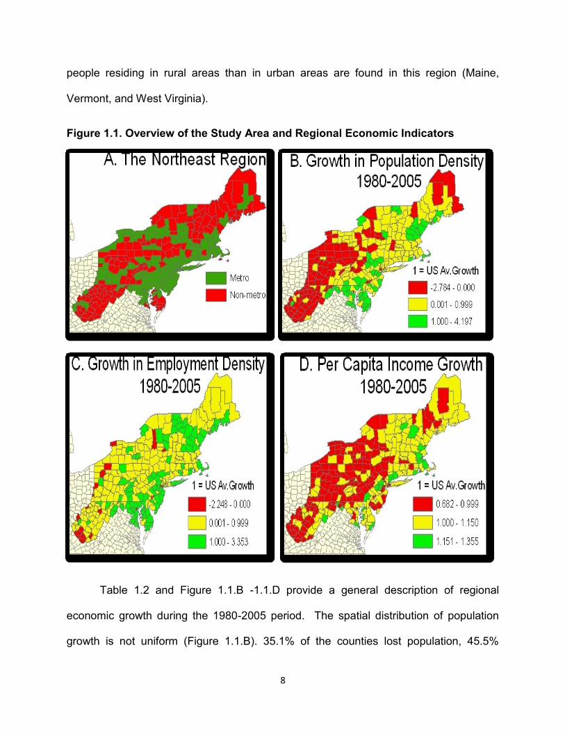
Figure 1.1. Overview of the Study Area and Regional Economic Indicators ................................................. 8

Figure 1.2. Comparisons of US and Northeast County Typology .................................................................. 9

Figure 3.2.1. Comparison of Traditional Export Theory and Amenity-Led Development .......................... 37

Figure 3.2.2. Amenities, Public Policy, and Regional Development ........................................................... 39

Figure 4.1. Climate Index .......................................................................................................................... 117

Figure 4.2. Natural Resource Amenities ................................................................................................... 117

Figure 4.3. Land Based Recreational Amenities ........................................................................................ 118

Figure 4.4. Water Based Recreational Amenities ..................................................................................... 118

Figure 4.5. Historical and Cultural Amenities ........................................................................................... 119

Figure 4.6. Winter Based Recreational Amenities .................................................................................... 119

CHAPTER 1: INTRODUCTION

1.1. Introduction and Problem Statement

There is no single way local policy makers can follow in developing the economy

of their region. They may follow single or multiple paths based on their endowments and

comparative advantages. They may build on natural resources, cultural resources,

human resources, local amenities, institutional facilities or location advantages. The

resulting direction of economic growth may involve manufacturing or supply chain

development, resource extraction, tourism development, educational development or

trade center development. The specific growth strategy followed by a specific region

depends on the social, economic, political, and environmental dynamics of the region in

question. In order to select and pursue a development path, policy makers must first

understand the possible growth paths that may be relevant for their region.

Interest in an amenity focused development strategy has exploded as

policymakers and community leaders realize that most natural resource based and

manufacturing jobs lost in recent decades will not return. Instead, these leaders are

looking inside their communities for new sources of economic growth. According to

recent white papers of the 2007 Farm Bills, the largest growth in rural population and

employment has generally occurred in areas which rely on nontraditional income

sources. These regions include areas that have either capitalized on natural resources

such as amenities and climatic conditions for recreation and retirement or areas that

have proximity to urban areas. In a 2006 report, the Outdoor Industry Foundation, for

example, found that active outdoor recreation contributes $730 billion to the U.S.

2

economy each year. For West Virginia, the study estimates that 61,000 jobs, $272

million in state tax revenue and $4.3 billion in sales are attributable to active recreation

in its wonderful, wild land. The type, quality and quantity of recreational activities

supported by the natural and recreational activities vary from region to region depending

on local climate, land, and water resources. In most cases they include, several of the

following: fishing, boating, paddling, and skiing, snowboarding, swimming, boating,

biking, hiking, hunting, golfing, wildlife viewing, camping and trailing. All levels of

government - federal, state, and local- and the private sector, are involved in providing

amenity-based services to thousands of people every day. For many rural counties,

these nature-based amenities are a major asset that gives the counties a comparative

advantage over other regions.

The increasing demand for the consumption of amenities is influenced by

decades of investment in transportation infrastructure which greatly enhanced the

accessibility of these amenities. Many rural communities are now connected by good

roads and the cost of isolation has been greatly reduced. The advance in information

technology has provided knowledge workers the flexibility to reside where they want.

The increase in income and changing preferences are two other factors that are

stimulating demand for amenities. Natural and built amenities, by boosting the quality of

life of regions, have become major forces behind the rural turnaround of the last

decade, including migration from urban to rural areas. Now we see different faces of

rural America: On one hand there are those areas which still depend on declining

extractive resources such as agriculture, mining, and lumber based manufacturing. On

the other hand, we find those which are within commuting distance to larger growing

3

cities which are benefiting from agglomeration spillovers. Others have transformed their

economies and are developing amenity based service industries (Lasley and Hanson

2003; Power, 1996; Deller, 2004).

Table 1.1. Comparison of Jefferson and McDowell County, WV, 1980-2005

Growth

Indicators

Jefferson County McDowell County

1980 2005 Growth

(%)

1980 2005 Growth

(%)

Population 30,434 48,542 59.5 49,724 23,794 -52.1

Jobs 8,385 15,486 84.7 14,561 5,318 -63.5

Per Capita

Income 7,394 32,240 336.0 7,230 18,136 150.8

Source: computed from Bureau of Economic Analysis data

A quarter of a century comparison of two counties- Jefferson and McDowell- of

West Virginia gives a good comparison of the different faces of rural America (Table

1.1). McDowell County is a good example of a declining extractive resource dependent

rural area. At its peak time in the 1950s, it was one of the important production centers

of the coal mining industry and a major player in the state’s economy. With the decline

of the coal industry everything started to fall apart. Its population decreased from

100,000 in the 1950s to an estimated 25,000 in 2005. In a quarter of a century (1980-

2005) alone, it lost more than 50% of its population and 63.5% of its employment. Even

though it’s per capita income increased by 150%, it is the lowest in the state and the

69th lowest among the US counties. About 33.8% of families and 37.7% of the

population were below the poverty line, including 52.5% of those under age 18 and

4

21.6% of those aged 65 or over. McDowell County was not able to transform its

economy and is lagging behind in almost every measure of economic activity.

Jefferson County, on the other hand, is an example of growing amenity based

service industry. The county is home to Harpers Ferry National Historical Park, which is

located at the confluence of the Potomac and Shenandoah Rivers. Due its ample

recreational opportunities and its proximity to the Washington, D.C., it has attracted

tourists and amenity migrants. In a quarter of a century (1980-2005) its population

increased by 59.5%. The ability of Jefferson County to transform its economy to an

amenity based service industry helped to almost double its employment and increases

its per capita income by 336%. Only about 7.2% of families and 10.3% of the population

were below the poverty line, including 11.4% of those under age 18 and 9.4% of those

ages 65 or over. Even though, these two West Virginia counties are found in

Appalachia, the difference in the development strategy they followed, the difference in

proximity to large urban centers, the demand for and supply of their amenities resulted

in two different growth paths. The story of Jefferson and McDowell Counties reflects the

different faces of rural America and the challenges and opportunities they face in their

development endeavors.

There is now a general understanding that natural and built amenities as quality

of life indicators are playing and will play important roles in rural development (Beale

and Johnson 1998; McGranahan 1999; Dissart 2005). Conceptually, amenities impact

regional growth by affecting growth in population, employment, income, and housing

values (due to land use changes for housing and recreational development). Several

past empirical studies have documented the relationship between the presence of

5

natural and built amenities within a region and economic growth by focusing on

population (or net migration), employment, and income growth (Deller et al. 2001, 2005,

2007 and 2008; Goe and Green, 2005; McGranahan, 1999; Nzaku and Bukenya, 2005).

In all the studies there is a clear and consistent positive connection between high

amenity areas and population growth while the relationship with employment is

relatively weak and less consistent. Very few studies address the income and amenity

relationship and it is difficult to generalize its impact based on them. Furthermore, there

has been a continuous debate whether amenities contribute to job growth directly or

indirectly through in-migration. At the same time awareness is growing that the

economic supply, not the physical availability of amenities, is important (Deller et al.

2008). The economic supply of amenities (accessible) and its impact on regional growth

vary significantly over space and are poorly understood. The different results seem to

emanate from ambiguity in the definition of amenity, the stated objectives, and the

method of analysis applied in the previous studies. These findings have created doubts

about the overall impact of amenities on regional growth (Dissart, 2007; Waltert and

Schläpfer, 2007).

State policy makers and local leaders need to have a full grasp of the relationship

between amenities and regional growth. Unless they have a better understanding of

what types of economic sectors and development programs are most appropriate in

attracting businesses, in alleviating poverty, and in influencing economic development,

they cannot design and follow a successful rural strategy. Thus, the determination and

documentation of population growth, employment growth, income growth, and the

distribution of amenity attributes that can provide the opportunity for economic growth in

6

rural areas can be used to design appropriate rural development programs. The

programs can create and retain rural employment opportunities, increase rural income

levels, and help keep population in rural communities. They can also enhance the

productivity and vitality of human and material resources, diversify the economic base of

rural areas, and allow greater adaptability of rural areas to changing external economic

and social forces.

This study will try to assess whether the 299 counties (148 are non-metropolitan)

in the Northeast1 (NE) region of the US can build and pursue a growth strategy that

depend on their local amenities (natural and built). Unlike past studies that implicitly

assume that the physical availability of natural amenities have a direct and independent

effect on economic growth, this study proposes that the availability of a high physical

amenity alone can only create the opportunity for economic growth. But to be an

effective development tool it should be coupled with factors that can exploit its

existence, encourage its use, and provide a comparative advantage. This requires

preserving local natural amenities, building recreational facilities, providing

transportation infrastructure, and promoting it in potential demand markets. To test the

relationship between amenities and such other factors, the study extends the models of

Deller et al. (2001, 2005, and 2007 ) and Nzaku and Bukenya (2005) by incorporating

interaction terms that account for the combined impact of amenities with proximity to

metropolitan areas and accessibility (interstate highway density). Furthermore, the study

also estimates a simultaneous spatial Durbin model using the two stage least square

method to capture the direct and indirect effects that are ignored in in most past studies.

1 The Northeast region of the US is defined here following the Northeast Center of Rural Development. It consists,

the 9 New England states and Delaware, Maryland, and West Virginia.

7

Table 1.2. Northeast Economic Growth, 1980-2005

Growth Indicator

Northeast Region Non-metro Northeast Region

Declining Growing Growing

Below US Average

Above US Average

Below US Average

Above US Average

Population 35.1%

45.5

19.4

44.5

40

15.5

Employment 6.7

61.2

32.1

7.4

64.2

28.4

Per capita income

0

46.8

53.2

0

52.0

48.0

1.2. Overview of the Study Area

The study area is the Northeast region of the U.S. as defined here. It is

composed of 12 states (Figure 1.1.A) and consists of all the counties in the states of

Connecticut, Delaware, Massachusetts, Maine, Maryland, New York, New Jersey, New

Hampshire, Pennsylvania, Rohde Island, Vermont, and West Virginia. It covers 6% of

US land area, 25% of total population and 11% of the non-metro population. The region

is appropriate for assessing the role of amenities and regional growth due to its diverse

spatial variation in economic growth and economic geography. According to the USDA-

ERS County Typology 1993, the region is highly urbanized with 50.5% of its 299

counties considered metro areas. The non-metropolitan areas are divided between 84

(28.1%) counties considered as adjacent to metro areas and 64 (21.4%) counties

considered as nonadjacent and completely rural. These 148 nonmetro counties can

also grouped into 13.4% of the counties considered as micropolitan areas with a central

city with at least 10,000 residents and 36.1% counties considered as noncore without a

central city of at least 2500 residents. Three of the five states in the U.S., with more

8

people residing in rural areas than in urban areas are found in this region (Maine,

Vermont, and West Virginia).

Figure 1.1. Overview of the Study Area and Regional Economic Indicators

Table 1.2 and Figure 1.1.B -1.1.D provide a general description of regional

economic growth during the 1980-2005 period. The spatial distribution of population

growth is not uniform (Figure 1.1.B). 35.1% of the counties lost population, 45.5%

9

recorded growth but below the national US average, and only 19.4% grew about US

average (Table 1.2). Most of the population loss counties are found clustered in the

Appalachian part of the region or in the northern part of Maine. Employment growth in

the region is not as low as population growth. Only 6.7% of the counties show negative

growth. More than 60% of the counties grew below national average while 32.1% grew

above national average (Table 1.2). The most encouraging regional growth indicator is

the growth in per capita income. 46.8% of the counties grew below the US average and

53.2 grew above it (Table 1.2). The spatial distribution of the of the regional growth

indicators in the non-metro counties in the region is not that much different from the

region as a whole (Table 1.2).

Figure 1.2. Comparisons of US and Northeast County Typology

As shown in Figure 1.2 below, the economic geography is diverse. 30.1% of the

NE counties are service dependent compared to 10.8% for all US counties. The NE

region is endowed with high human capital as reflected by few counties with low levels

of education (6.4% of the counties with low education compared to 18% for US).

10

Although, the region as a whole has very few poverty persistent counties compared to

the US, it has the highest population loss counties (21.7%) due to out-migration.

Most of the population loss counties are found in the Appalachian part of the NE,

counties found in West Virginia and Pennsylvania, upstate New York, and Maine

(Figure 1.1.B). In the northeast region, with the exception of very few counties, all metro

and nonmetro counties in the region lost population aged 25-44 during the period of

2000-2005 (Yang and Snyder, 2007), which indicates the region is losing the most

productive part of its population. In general, declining farm employment and lack of

natural amenities are cited as the main reasons for population loss (MaGranahan and

Beale, 2003). As shown in Figure 1.2, the Northeast region doesn’t have any farm

Table 1.2. Northeast Public and Private Natural Resources and Recreational Facilities

State Wild Acres

FS-NF Acres

NPS Acres

COE Acres

FWS Acres

NWSR Miles

NRI River Miles

State Park Acres

Private Recreation Business

Public Recreation Facility

CT 0 0 7734.59 3232 712.88 0 115 175860 1419 942

DE 0 0 0 0 26700.15 0 298 18189 313 175

ME 19386 49166 90590.39 0 45404.54 95 1318 285264 1328 1030

MD 0 0 69927.12 15 40731.32 0 784 292279 1778 1406

MA 2420 0 55818.57 5206 12472.26 0 226 587558 2666 1942

NH 102126 720016 10461.23 3436 5859.41 15 1656 341301 1115 1081

NJ 10341 0 53175.23 0 60678.58 16 479 90693 3029 959

NY 1363 13232 95655.92 0 26704.06 39 2812 20046 5854 2424

PA 9705 513001 109172.7 12418 9773.59 55 580 283001 4756 5823

RI 0 0 4.56 0 1523.39 0 34 8748 485 1031

VT 59536 340130 14878.84 4961 6409.48 0 855 72610 694 981

WV 80682 1024876 80829.89 2542 1642.96 17 1472 127811 570 2844

Total 285559 2660421 588249 31810 238612.6 237 10629 2303360 24007 20638

Compiled from the NORSIS data base

dependent county. All the counties in the region also score from moderately low to

moderately high (-1 to 1 standard deviation from the mean) in the USDA-ERS natural

11

amenity scale. In fact, the region is endowed with moderate natural amenities that are

not part of the natural amenity scale. According to the National Outdoor Recreation

Statistical Information System (NORSIS, 1997) of US- Department of Agriculture, Forest

Service, the region is home to five national forests (FS-NF) that cover more than

2,660,421 acres, 285,559 acres of wilderness, 20% of the 391 attractions managed by

the national park system (NPS) in 588,249 acres, and 238,612 acres of wild life

attractions managed by Fish and Wild life Services (FWS). The region also has 31,810

recreational acres of Corps of Engineers (COE), 237 miles of National River System

(NWRS), and 10,629 river miles in the Natural Reserve Inventory (NRI). All these

federally owned and managed natural endowments provide a wide range of recreational

activities like fishing, wildlife watching, hunting, snowboarding, boating, swimming,

golfing, camping and hiking in more than 20,000 built recreational facilities. An

estimated 700 state parks with more than 2,303,360 acres and 24,007 recreational

private businesses also give the region additional attractions and competitiveness. Even

though, the current NORSIS data base is not yet disseminated, the above data is

expected to change.

State and local governments all over the US are using quality of life amenities as

one of their competitive edges. Consequently, local investment in parks and recreation

increased by 121% during the period of 1992- 2006. The rate of local development

based on amenity-led development depends on local policy, the demand for and supply

of amenities, spatial distribution of the counties, and the interdependence of regional

growth factors (population density, employment density, and per capita income).

12

1.3. Objective of the Study

The overall objective of this study is to provide policy makers with information on

the role of natural and recreational amenities in rural economic development in the

Northeast region. The specific objectives are to:

1. Develop a database of natural and built amenities, economic, social, fiscal and

demographic variables of the Northeast region.

2. Estimate the impacts of regional economic growth and identify and measure the

impacts of an amenity-led development strategy as reflected by growth in

employment density, population density, and per capita income as the result of

natural and built amenities in the Non-Metro areas of the Northeast region.

3. Identify the spatial distribution of amenities in the growth process.

4. Evaluate the role of proximity to demand market and accessibility in following

amenity-led development.

5. Draw policy implications about amenity-led development strategies for rural

economic development.

1.4. Hypotheses The central focus of the study is to examine how amenities, controlling for a

range of socio-demographic and growth variables, affect changing levels of economic

development as expressed by growth in population and employment densities, and per

capita income. Hence, the study attempts to empirically test economic relationships

between growth factors and natural and built amenities in a regional growth setting. In

establishing these relationships, this study, following previous literature makes the

13

following basic assumptions. Utility-maximizing households migrate in search of utility

derived from the consumption of market and non-market goods, and profit maximizing

firms on the other hand become mobile when looking for regions that have lower

production costs and higher market demand. Based on these free migration

assumptions and rational expectations, the following relationships are hypothesized.

Hypothesis #1: Regional growth, as measured by growth in population density,

employment density, and per capita income, is conditional on local natural and built

amenities.

Hypothesis #2: Pursuing amenity-led development requires proximity to demand

market (location matters) and accessibility factors, such as road density.

Hypothesis #3: Growth is conditional on initial conditions.

Hypothesis #5: Growth is conditional and affected by economic activities in

surrounding counties.

These five hypotheses will be empirically tested using Northeastern regional

data. To test these hypotheses, a spatial and non-spatial simultaneous equations model

of growth in population and employment density, and growth in per capita income is

used. The empirical methodology to test these hypotheses is discussed in detail in

Chapter IV.

14

1.5. Methodology

In this study a regional lag adjustment model will be used which is basically

rooted in a compensating differentials framework that characterizes migration as a

spatial response to economic opportunity, in the form of employment, higher wages,

and/or other means of advancement, and personal preference for natural and built

amenities, lifestyles, and other quality of life improvements. It is also an application of

the partial adjustment model which uses a simultaneous-equation system that

expresses the interdependencies among growth in population and employment density

and growth in per capita income. In this study, a three equation regional adjustment

model will be used wherein changes in population density, employment density, and per

capita income are endogenously determined in the presence of natural and built

amenities.

The model builds on the spirit of Carlino and Mills (1987), and extends the

models of Deller et al. (2001, 2005, and 2007) and Nzaku and Bukenya (2005) by

incorporating interaction terms to test for the combined impact of amenities with

proximity to metropolitan areas and accessibility (interstate highway density). Spatial

and non-spatial models will be constructed and estimated. A national dataset of all

nonmetro counties will be used in the non-spatial empirical estimation of the model with

amenity slope shifters for the Northeast region. The same model will also be separately

estimated for the 148 nonmetro counties of the Northeast region. The nonspatial models

will be estimated by three stage least squares. Furthermore, to capture the direct and

indirect effects, a simultaneous spatial Durbin model will be estimated using a two stage

15

least squares method for the 1980-2005 period. Even though the focus of the study is

the Northeast Region, the study will use both datasets.

1.6. Organization of the Study

This study is comprised of five additional chapters. Chapter 2 provides an extensive

review of literature in defining and measuring amenities, the relationship between

amenity and regional growth, and relevant modeling approaches. Chapter 3 provides

the theoretical foundation for modeling amenities and economic development decisions.

Chapter 4 discusses specification of the empirical model and of the types and sources

of data. Chapter 5 provides analysis of results from model estimation and a summary of

the major findings of the study and its policy implications. Finally, Chapter 6 provides a

summary, conclusions, and recommendations for policy measures to better preserve

and utilize natural assets

16

CHAPTER 2: LITERATURE REVIEW

The purpose of this chapter is to review the most relevant literature on amenities

(natural and built) and rural development. The chapter is divided into four sections. The

first section defines amenities and describes the potential relationship of amenities and

rural development. The second section is devoted to describing how amenities are

measured and used in different empirical studies. In the third section, the impact of

amenities on economic growth and income distribution (two aspects of economic

development) will be discussed. Finally, in the fourth section, methodologies used in

amenity related empirical studies will be reviewed.

2.1. Amenities and Economic Development According to Shaffer, et al. (2006) most of the time economic growth and

economic development are used interchangeably. Though the concepts are related they

are different. Economic growth is about the growth in employment, income, and

resources of production. Economic development goes beyond economic growth to

incorporate the institutional and structural change in the capacity to act, innovate, and

move forward in all aspects of life. Therefore “economic growth can occur without

development, and development can occur without growth” (p.61).

In the literature there are several related but somehow different definitions of

amenities. Amenities can be broadly defined as non-marketed qualities of a region that

make it an attractive place to live and work (Power 1988). The term amenities is also

defined as any attribute of a geographic location for which a resident or potential

17

migrant would be willing to pay, either through higher housing costs, lower wages, or

other location-specific costs, but for which there is no market through which the

individual can directly purchase a given amount of that good (Judson et al.1999). It has

also been used to refer to the available stock of natural resources such as forests,

mountains, hills, lakes and rivers (English, Marcouiller, and Cordell 2000) and/or to the

availability of opportunities for recreational activity (Beale and Johnson 1998).

Amenities provide benefits to people directly through direct consumption and to

firms by entering directly or indirectly into the production function of certain aspects of

land, natural resource and human activities. In this study, Power’s (1988) definition is

adapted and modified to define natural and built amenities as “natural and built qualities

of a region that make it an attractive place to live and work”.

The above definition gives the flexibility to include some of the marketed amenity-

based recreational attributes of a region along with the nonmarketed natural attributes.

Examples of amenities are wildlife and flora, climate, recreational areas (golfing, skiing,

fishing, hunting, hiking, and swimming) cultivated landscapes, unique settlement

patterns, historic sites, and social and cultural traditions.

According to Green (2001) and OECD (1994), there are four potential

relationships between amenities and development. The first possible relationship is that

development can lead to the destruction of amenities. This is the case where economic

growth leads to more pollution and congestion due to rapid population or employment

growth in a region that contains a natural resource area. On the other hand, it is also

true that in some cases the lack of economic development can lead to the destruction of

18

amenities. One example of this type of relationship is the effects of depopulation on the

maintenance of historical buildings and scenic landscapes. A third possibility is that

preservation of amenities may lead to non-development. One controversial example of

this might be the “potential curtailing of economic development” through designating a

land area as a critical habitat for endangered species. Duffy-Denno (1997a), Lewis et al.

(2002), and Keith and Fawson (1995) assessed the economic implications of wilderness

and conservation of lands in different regions of the US. The results of these studies

show no evidence of curtailing of economic growth due to the preservation of amenities.

The final possible relationship between amenities and development is that

preservation or promotion of amenities leads to development. An example of this type of

relationship might be eco-tourism projects that preserve the natural environment that

help attract retirees and firms to move to the area. In this case amenities are used as

any other goods for consumption or production to enhance the well being of the local

population and create economic development. The main focus of most of the studies in

the literature is to empirically test this possible positive relationship between amenities

and economic development, specifically economic growth or/and income distribution.

This study will follow the literature and try to assess the role of natural and built

amenities on rural development.

2.2. Measuring Amenity Attributes

Measuring amenities has been a challenge to researchers. The main problem is

that there is no market to derive a value. Furthermore, as discussed above, the

definition of amenities is becoming broad and encompasses almost any attribute found

in a location. In fact, the main sources of data for most studies, the National Outdoor

19

Recreation Statistical Information System (NORSIS), which is compiled by the USDA

Forest Service, has more than 300 amenity related variables.

Three approaches can be identified in the literature in measuring amenity

attributes: single factor, a summary index (single index) approach and an aggregate

factor score approach. The single factor approach tries to include all relevant amenity

attributes in the model estimation. Duncombe, et al. (2000) applied this approach by

including five amenity variables in their analysis of elderly migration. McGranahan

(1999) used six amenity measures to study the population and employment changes in

rural America during the 1970-1996 period. Others, like Roback (1982, 1988), and

Carlino and Mills (1987), used number of sunny days as an amenity attribute in their

studies. The advantage of the method is that it is straightforward for doing marginal

analysis and interpreting the results as any other variable in the model. Its drawback is

that you can’t include all the relevant variables which may lead to omitted variable bias

and, on the other hand, if you try to include all variables, it may lead to multicollinearity

problems.

The summary index approach is an effort to define natural amenities as a single

index of different amenity attributes. Nord and Cromartie (1997) produced the summary

index to represent natural amenities in rural counties. Their summary index consisted of

mild sunny winters, moderate summers with low humidity, varied topography,

mountains, and the abundance of water. McGranahan (1999) generated a single index

called a natural amenity index by summing six amenity measures: average January

temperature, average January days with sun, low winter-summer temperature gap, low

average July humidity, topographic variation, and water areas. Even though it is a

20

broader measure than the single factor, the single index is criticized for being uni-

dimensional in representing the very diverse nature of amenity distributions (ignores

built recreational amenities and historical amenities among others) and for the

subjectivity incorporated in the decisions about which amenity attributes should be

included to develop the index. But despite this weakness, McGranahan’s (1999) natural

amenity index is the most widely used amenity measure in empirical studies.

The aggregate factor score approach is the latest trend in measuring amenities.

It is an effort to reduce a wide array of natural amenity attributes into multiple but similar

groups. The Principal Component Analysis (PCA) is a method of combining a set of

related variables into a single scalar measure. Many recent studies have evaluated the

economic impacts of natural amenity attributes using the Principal Component Analysis

(PCA). Goe and Green (2002), using PCA, reduced thirty two amenity attributes into

four groups: climate, land, water (two distinct sub groups of river and lake based),

outdoor recreational amenities (two distinct categories warm and cold weather based),

and historical/cultural amenities. Following the same approach (PCA), Deller et al.

(2005, 2007) examined the economic effects of five amenity measures (created from

more than 50 different attributes): climate, urban facilities, land, water, and winter

amenity attributes. Finally, Monchuk (2003) reduced about fifty natural amenity and

recreation site variables into five distinct categories unique to the states of Kansas,

Minnesota, Missouri, Nebraska, North Dakota, and South Dakota. In all the above

studies there is no uniformity in including or grouping the different attributes to create an

index. For example, in developing the land index, Goe and Green used four while Deller

et al. used sixteen different attributes.

21

The aggregate factor score approach is also subjective as is the single index

approach and the final measures (factor scores or principal component scores) may not

be easy to interpret. The use of aggregate factor scores, however, can allow

researchers to examine multidimensional aspects of natural amenity attributes (English,

Marcouiller, and Cordell 2000; Deller et al. 2005; Marcouiller et al. 2004).

2.3. Review of Factors Associated With Amenity and Rural Development Numerous studies (Deller et al. 2005, 2007; Monchuk, 2003; McGranahan 1999;

Rudzitis, 1999; Gottieleb, 1995; Roback, 1982 and 1988) have documented that

different types of amenities play an important role in economic development. Several of

these studies link economic growth trends directly to some measure of natural or scenic

amenities.

In seminal studies of the role of amenities, Roback (1982 and 1988), assessed

the impact of amenities on wage rates and land rents in selected US cities. Her measure

of natural amenity was climate. She found that climate and other quality of life factors

are capitalized into wages and housing values and rents. People who prefer to live in

higher amenity areas are willing to pay high housing values or rents. On the other hand

it is expected that workers would be willing to receive lower wages in a location with

high quality of life amenities. Hoehn et al. (1987) also found statistical differences in

housing prices and wages due to location specific amenities. On the impact analysis of

state parks on the economies of the counties of the inter mountain west, Duffy-Deno

(1997b) found a relatively weak effect on county level population and employment growth.

All the above studies used a single measure of amenity attribute of a location. In reality

22

a region could be endowed with multiple natural and built amenities that can influence

the regional economy.

One way through which amenities affect firm location is through compensating

wage differentials. If households require higher wages to live in low-amenity locations,

the firms in those locations must have some productivity advantage to be able to pay

the higher wages. Conversely, if households are willing to accept lower wages to live in

amenity locations, firms would follow workers to those locations unless there are some

offsetting disadvantages in those places. Gottieleb (1995) addressed the issue of

amenities in firm location decisions. His model assumed that there is a direct link

between residential amenities and firm location. Thus, the study omitted population

(labor force) aggregates entirely, and focused on the long-run relationship between

residential amenities, traditional business factors and employment location. He found

that residential amenities are important factors in business location.

The widely cited work of McGranahan (1999) was a major contribution to the

amenity literature in the 1990s. In the descriptive analysis, a positive relationship was

found between natural amenity scale with rapid rates of population growth and

employment change. High amenity counties had an average of three times as many

jobs during this period than those that scored low on the amenity scale. However,

employment change was much more variable during this period than population

change, especially for high amenity counties. But in this simple descriptive analysis it was

assumed implicitly that the physical availability of high amenities is related to regional

growth without consideration of their economic supply. The analysis does not make any

23

distinction between completely rural and isolated areas with those that are more

accessible and close to high population centers.

In a similar study, the Center for the Study of Rural America used this same

amenity measure to estimate the effect of amenities on employment growth while

controlling for a much broader set of characteristics (Henderson and McDaniel, 1998).

The results verify that while scenic amenities are associated with employment growth,

the impact is quite small. White and Hanink (2003) using the same amenity scale but

taking into consideration the impact of accessibility found that the accessibility of places

with relatively high natural amenity endowments is a necessary factor in those

amenities’ ability to contribute to economic growth in the Northern Forest area of the

Northeast region of the US. McGranahan (1999) also neglects the role of built amenities

that take advantage of the physical availability of natural amenities (parks, play grounds,

ski resort, golf courses, and others).

Deller et al. (2001, 2005, and 2007, 2008) expanded the single dimensional

natural amenity scale to multiple dimensions that include built-in amenities. All these

studies further confirmed the positive relationship between amenities and regional

growth. Beyond population and employment growth these studies addressed the issue

of income growth. Although climatic condition had a strong influence on population

change, it had a relatively minor effect on employment and per capita income growth.

Similarly, water amenities were significantly related to population change, but not to

employment and per capita income growth. Even though these studies used more

expanded measures of amenities they limited the study to population, employment, and

income of regions. One of the greatest assets of rural communities, land, which is also

24

affected by amenities and which in turn could have a feedback effect into these growth

indicators is not included in the analyses. Furthermore, like McGranahan (1999) their

analysis doesn’t make any distinction between completely rural and isolated areas with

those that are more accessible and close to high population centers (the issue of

accessibility and proximity is not adequately addressed).

The role of spatial distribution of amenities and its impact on the local economy is

addressed only in a very few studies. Regions with very low amenities can benefit from

the presence of high amenities in their surroundings. Household and firms can find it

cost effective to live in low amenity areas as long as there are easily accessible ample

amenities in surrounding areas. Monchuk (2003) evaluated the role of surrounding

counties’ amenities for a county in six states of the Midwest. Using spatial lags of five

amenity indices, he found that surrounding counties amenities are more important to

employment growth than the local amenities in his study area. Deller et al. (2008)

constructed five spatially weighted, narrowly defined specific recreational measures to

estimate the role of own and adjacent county amenities on growth of per capita income.

They used a neoclassical growth model and found that higher levels of developed

resources, such as tourist attractions, amusement parks, zoos, and campgrounds have

a positive impact on per capita income growth. But they also found that public acreage

lands for recreation have a negative impact on growth. One common thing these two

articles show is that the availability of amenities in surrounding counties matter in rural

development. Empirical studies that ignore this spatial issue could suffer from omitted

variable bias.

25

Deller et al. (2005, 2007) using their expanded five dimension amenity attributes

found that amenities are related to economic growth. Although climatic condition had a

strong influence on population change, it had a relatively minor effect on employment

and per capita income growth. Similarly, water amenities were significantly related to

population change, but not to employment and per capita income growth.

The Economic Research Service (ERS, 1997) identified 514 in 1970 and 190 in

early 1990s as retirement counties. Most of these non-metro retirement counties were

near metro areas, whose more robust economies helped them outperform other non-

metro counties in attracting and retaining people of all ages, including the elderly. Rural

retirement counties with substantial net in-migration of the elderly have enjoyed

significantly more rapid population and employment growth than other types of metro

and non-metro counties since the 1970s. The influx of retirees is also associated with

increased family incomes, reduced unemployment rates, and greater economic

diversification in rural areas.

However, others have also looked at this relationship from a different perspective

and found different results. Duffy-Deno (1997a) examined whether local economies may

be adversely affected by designation of federal-owned wilderness in the eight states of

the intermountain western United States. He found no evidence that the existence of

federal wilderness was directly or indirectly associated with population or employment

growth between 1980 and 1990. This conclusion is further reinforced by Lewis et al.

(2003) findings of no evidence of lower wages due to alternative public land

management policies in the Northern Forest region which stretches from northern

26

Minnesota to Maine. Even though, they used different data sets and models, their results

are a direct opposite of the negative effect found by Roback (1982 and 1988).

In an earlier study, Lewis et al. (2002) also assessed the impact of access to

public conservation lands on the Northern Forest region to migration or employment

growth of the region. They used a simultaneous regional growth model of net migration

and employment. They found that the conservation land share had a positive direct but

relatively small effect on net migration. On the other hand no significant direct effect on

employment growth was detected. But, since net migration positively influenced

employment at the end of period, we can conclude that it had an indirect effect on

employment. State level studies in Alabama (Nzaku and Bukenya, 2005a) and Utah

(Keith and Fawson, 1995) have also found no evidence that suggests a positive role of

amenities on economic growth.

2.4. Methodological Issues

There are, broadly speaking, two empirical approaches, Regional economic

models and hedonic pricing models, that look to the impact of amenities on economic

growth. Both of these models use an equilibrium modeling framework. The hedonic

models show that a wide variety of local amenity attributes are partly capitalized into

local wages and land rents. Hedonic models indicate that money wages can be offset in

places by environmental and other amenities. The uneven abundance of such

amenities, therefore, can explain relatively uneven wages and rents in the contemporary

economies (Roback 1988, 1982).

Regional economic models aim to identify the direct and indirect effects of

amenities on change in population, employment and income, and to capture interactions

27

between these variables. They are usually designed as simultaneous equations models

and such models are used in this study. Models of this type have traditionally been used

to explore empirically whether people follow jobs or jobs follow people. The model was

first developed by Steinnes and Fisher (1974) and used it in their classic study to

explain the intra-urban location of residents and employment in a two-equation

microeconomic model. The models were further refined and operationalized by Carlino

and Mills (1987), Deller (2001), and many others.

These models are also called lag adjustment models because in a way they are

a compromise between the equilibrium and disequilibrium perspectives of regional

development and migration. While they maintain the equilibrium assumption, they also

recognize that the impact of the dis-equilibrating forces in the region. The models

implicitly assume that the real equilibrium point is unknown and if there is one, a

substantial lag is needed to move towards it. They operate on the assumption that

there is an endogenous or bi-directional process at work in the various regions, where

employment growth (labor demand) drives population growth and population growth

(labor supply) drives employment growth. In general, researchers first assume that firms

(employment) and households (population) are geographically mobile. Firms move to

maximize profits and households to maximize their utility. Economic opportunity and

personal preferences are assumed to be the motivating factors behind the movement of

people and firms.

Consumer utility is derived from goods and services as well as from non-market,

location-specific amenities. Firms maximize their profits by optimizing production costs

and choice of a regional market. The result is an adjustment process in which “firms

28

enter and leave regions until profits are equalized among regions at competitive levels,

and households migrate until utility levels are equalized at alternative locations” (Carlino

and Mills, 1987, p. 40). This is an improvement from the traditional regional models that

depend only on economic opportunity and ignore the role of personal preferences. But

earlier models account for the role of amenities either by dummy variables or climate.

Graves and Muser (1993) were among the first to critique these models and point out

the bias that can be created by “any unmeasured stable differences between

locations…. such as land rent and natural amenities.” In response, recent studies started

to include explicit measures of natural amenities. One final major improvement was the

work of Deller et al.(2001) which added a third equation to capture the income

differences in locations and its impact on the growth process.

Many past studies have addressed the relationship between amenities and

economic development using regional simultaneous equation models. Rudzitis (1999)

examined growth in and around counties with federally designated wilderness and

found that employment did not explain migration, while migration did explain

employment. Vias (1999) also looked at 254 non-metropolitan counties in the Rocky

Mountain West for three time periods, the 1970s, 1980s and 1980-1995 and found that

population was the driving force for employment growth, but there was also an inverse

relationship between employment and population. As employment declined, population

increased.

Duffy-Deno (1997b) following a similar approach examined whether local

economies may be adversely affected by designation of federal-owned wilderness in the

eight states of the intermountain Western United States. He found no evidence that the

29

existence of federal-owned wilderness was directly or indirectly associated with

population or employment growth between 1980 and 1990. The two equation system is

expanded to a three equation system. Recently, Deller et al. (2001, 2005, 2007) applying

the same approach have found that amenities have positive impacts on economic

growth.

In all the above studies the role of space and spatially distributed amenities was

ignored. Nzaku and Bukenya (2005b) introduced a spatial lag component to capture the

spatial dependence and extended these models. Recent works of Deller et al. (2005

and 2007) also used a spatial error model to capture the unobserved spatial distribution

of amenities on the region. But both the extended works of Deller et al. (2001, 2005,

and 2007) and Nazaku and Bukenya (2005b) never tried to estimate the spatial impact

of surrounding county amenities estimated on regional economic growth. In the

presence of spatial dependence on the distribution of amenities, ignoring this spatial

effect can lead to biased estimators. Thus, their studies reflect only the direct effect of

amenities on the regional growth indicators ignoring the spillover effects coming from

surrounding counties.

Furthermore, they estimated a reduced form which captures the total effect. They

did not attempt to estimate the impact of amenities in the structural equations. If

amenities impact population growth and population growth positively affects

employment and income growth, amenities may have an indirect effect on employment

and income growth even if they do not have direct effects. This study will use a spatial

simultaneous equation model to capture both the direct and indirect effect of amenities.

30

2.5. Summary and Shortcomings of Past Studies

The contribution of studies in terms of refining the definition of amenities,

measuring amenities and evaluating their direct effects on a regional economy is

enormous. The works of Power (1988 and 2005), Roback (1988 and 1982),

McGranahan (1999), and Deller et al. (2001, 2005, 2007, 2008) are some of the major

contributions to our understanding of the role of amenities in regional development. But

additional work is required to more fully understand and evaluate the overall effects of

amenities on regional development.

Past studies assume that amenities have a direct and independent effect on

economic growth, but in reality the availability of high amenity levels alone can only

create the opportunity for economic growth. But to be an effective development tool it

should be coupled by factors that can exploit its existence, encourage its use, and give

it a comparative advantage. For example, two counties with more or less similar

amenities could have a difference in their development due to the difference in

infrastructure, local policies and economic geography. Therefore, there is a need to

account for these factors in empirical studies. An effective development tool for rural

areas should be able to provide the optimal mix of policies to complement the particular

set of amenities possessed by a region.

With the exception of Nzaku and Bukenya (2005b) and Deller et al. (2005) in

almost all past studies the role of space is ignored. Spatial autocorrelation is not

controlled. Ignoring spatial autocorrelation and estimating using OLS leads to inefficient

standard errors which in turn affects the significance levels of the variables (Wooldridge

31

p.6 and 134). Predictions made based on this will be misleading and may have undesired

policy implications.

In terms of population growth, amenities have been found to contribute rather

than detract from it. Furthermore, the extent to which an amenity exerts a positive effect

on the locale, both in terms of attracting people to that county and, in turn, its

development depends heavily on people’s preference for a particular amenity.

The direct impact of amenities on employment and income growth is mixed. In

most studies it is positive but small. In others it is found to have no effect. This may be

explained in part by the desire of people to forego income and employment benefits in

higher amenity areas. But as discussed above many of the studies have ignored the

indirect effects of surrounding county amenities by only focusing on own county amenities.

Thus, it is difficult to evaluate the overall effects of amenities on regional growth. This

study attempts to extend past studies further not only by capturing the total effects of

amenities but also by explicitly evaluating the role of proximity to the demand market

and accessibility to amenities. Furthermore, using a spatial Durbin model, the study will

estimate the impact of surrounding county amenities on regional economic growth.

32

CHAPTER 3: THEORETICAL MODELS OF AMENITIES AND REGIONAL

DEVELOPMENT

3.1. Household and Firm Location

Regional development to a great extent is determined by the location decisions

(mobility behavior) of firms and households. Both these behaviors impact regional labor

markets by demanding and supplying labor. Amenities,2 which are location specific, play

a role as one of the important determinants of location decisions (Roback, 1982 and

1988). Thus, closer understanding of the relative importance of amenities as a

determinant of mobility behavior serves as a starting point for understanding the

variation in development in a region.

This section presents a model to analyze the interaction between the location

decisions of firms and households and their effect on spatial variations in economic

development. The model was originally developed by Roback (1982) and will be

discussed below with minor changes. It is a simple general equilibrium model which

allows for wages and land rents to interact in the location decision of households and

firms.

The model is based on the following assumptions: (1) locations differ by natural

and built amenities (a) ; (2) labor and capital move freely from location to location with

zero movement costs; (3) Workers (households) are assumed to be identical in tastes

and skills while firms are identical in technology and are subject to constant returns to

scale; (4) households in each region produce and consume a composite commodity

2 Amenities are defined as in chapter two as “location specific natural and built attributes that make a place an

attractive place to live or work”.

33

(Hicksian consumption bundle), X, whose price is determined by world markets and will

be taken as the numeraire; (5) each household supplies a single unit of labor

independently of the wage rate (w) and; (6) the supply curve for land is upward sloping3.

3.1.1. The Household’s Location Decision

At each location, the problem of the representative household is, given the

quantity of a in its location, to choose quantities of X, and the residential land (lc ) to

satisfy the budget constraint. At each location, a household solves the following utility

maximization problem:

(3.1.1) Max U(x, lc ; a)

s.t. w + I = x + r lc

The wage rate is denoted by w, the rental payment is denoted by r, and I is non-labor

income and is assumed to be independent of location.

The optimal solution of (3.1.1) yields the demand functions for residential land and the

composite good:

(3.1.2) lc d = lc (w, p; a, I)

(3.1.3) xd = x(w, r; a, I).

Substituting equations (3.1.2) and (3.1.3) into (3.1.1), we get the indirect utility function

which gives the maximum utility attainable given the wage, the residential

land price, the level of amenities, and the nonwage income. Thus, households choose

residential locations to maximize utility V (w, p; a, I) by considering the trade-offs

3 According to Roback (1982), a rising supply price of land assures a boundary on the size of the city (p.1259).

34

between wage (w), residential land price (r), and amenities (a). Since households are

assumed to be completely mobile and migration is assumed to be costless, equilibrium

for households requires that wages and residential land prices adjust to equalize utility

in all locations. The market equilibrium condition for utility maximizing workers is given

by:

(3.1.4)

Where is the constant utility level, exogenous to individual locations. The

equilibrium condition implies that utility at all locations is equalized in an interregional

equilibrium, with the common level of utility equal to some constant k. If this doesn’t

happen, some workers would have an incentive to move to maximize their utility. One of

the main properties of the indirect utility function is ∂V/ ∂a > 0 because higher amenity

levels increase utility.

3.1.2. The Firm’s Location Decision

Firms choose production locations to minimize total cost of producing the

composite good X = f (n, lp, a)4 by considering the tradeoff between input prices, given

the quantity of a (a can be productive or unproductive in the production process) in the

location. The production function is assumed to exhibit constant returns to scale and

diminishing marginal returns to each factor. So, at any given location, a firm chooses

the best combination of labor (n) and land used in production (lp) to minimize the total

production cost (r and w are price of land and wage rate respectively):

(3.1.5) min wn + rlp

4 According to Roback (1982, p.1260) “X is a function of capital…..but since capital is perfectly mobile and is

uninfluenced by amenities, its rate of return will be equal in all places…….capital…..optimized out of the problem”.

35

s.t. X = f (n, lp, a)

Costless mobility and open entry assure that firms everywhere produce at a minimum

cost and that marginal cost equals unit price. The optimal solution of (3.5) yields the

demand functions for land in production and labor:

(3.1.6) lp = lp (w, r; a)

(3.1.7) nd = nd (w, r; a )

Equilibrium for firms requires that wages and rents adjust to equalize unit cost in all

locations which has to equal product price of unity:

(3. 1.8) C (w, r; a) = 1

This condition assures the spatial equilibrium of firms. If this does not happen, some

firms would have an incentive to move to their capital to maximize their profits.

3.1.3. Interactions between Location Decisions of Households and Firms

If a region wants to attract new firms and households, the amenities in the region

should insure that the cost per unit is below unity (C (w, r; a) ≤ 1) and the indirect utility

should be above the regional desired equilibrium ( . This will give the

region cost and quality of life comparative advantage to attract new firms and

households until it is eventually equalized. For a given set of amenities, an increase in

land price must be offset by an increase in wages to maintain consumer indifference.

Increases in wages must be offset by reductions in rent to maintain unit costs equal to

unity. The equilibrium conditions for firms and households, (3.1.4) and (3.1.8), together

determine the equilibrium level of wage and land price. That is, the interaction between

36

the two sides of the markets determines the equilibrium level of wages and housing

prices. In equilibrium, locations with higher amenities will have higher land prices and

lower wages. Regions with lower amenities will have lower land prices and higher

wages.

3.2. Traditional Export Theory and Amenity-Led Development

The central focus of this study is to examine how amenities, controlling for a

range of socio-demographic and growth variables, affect changing levels of economic

development as expressed by population, employment, and income growth. The figure

below, which is adapted from Power (1996), captures how amenity led development

works and compares it with the traditional economic base theory. Power suggests that

the logic of amenity-led development turns traditional export base theory on its head. He

compares what he refers to as the extraction and environmental views of the economy.

The extraction view of the local economy assumes that to spur development it is

necessary to extract resources from the natural environment for export to external

markets. The income generated from this export activity is multiplied throughout the

economy and puts additional people to work.

The environmental view of the local economy argues that environmental quality

is at the root of economic development. Improvements in environmental quality attract

workers and businesses to move to the area and increase the amount of retirement

income. The new economic activity leads to diversification of the economy and

additional jobs and income.

As discussed in Chapter 2.1, Green (2001) and OECD (1994) presented four possible

relationships between amenities and development. One of the four possible

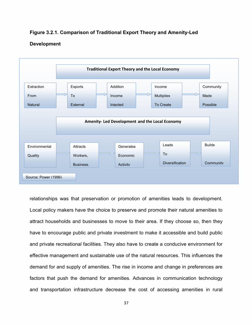
37

Figure 3.2.1. Comparison of Traditional Export Theory and Amenity-Led

Development

relationships was that preservation or promotion of amenities leads to development.

Local policy makers have the choice to preserve and promote their natural amenities to

attract households and businesses to move to their area. If they choose so, then they

have to encourage public and private investment to make it accessible and build public

and private recreational facilities. They also have to create a conducive environment for

effective management and sustainable use of the natural resources. This influences the

demand for and supply of amenities. The rise in income and change in preferences are

factors that push the demand for amenities. Advances in communication technology

and transportation infrastructure decrease the cost of accessing amenities in rural

Extraction

From

Natural

Environment

Environmental

Quality

Attracts

Workers,

Business,

and Retirees

Generates

Economic

Activity

Leads

To

Diversification

Builds

Community

Addition

Income

Injected

Community

Made

Possible

Income

Multiplies

To Create

Jobs

Amenity- Led Development and the Local Economy

Traditional Export Theory and the Local Economy

Source: Power (1996)

Exports

To

External

Markets

38

areas. Amenity focused public policy, the supply of, and demand for amenities create a

conducive environment for households and firms to move to the area and influence the

local labor market. The move of firms increases the demand for labor, while the move of

households influences the supply of labor. Both the demand and supply of labor

determine the local wage rate (Figure 3.2.2).

There are several ways in which local amenities impact local economic development.

Power (2005) and Gottlieb (1994) discuss the process of how amenities impact a local

economy. Generally, there are five types of groups that can influence amenity-led

regional development: tourists, second-home owners, retirees, working - age in-

migrants and relocating/expanding/new businesses. First, amenities draw tourists, i.e.,

temporary visitors who want to enjoy local amenities. Businesses focused on serving

these visitors’ needs may be created or expanded. Some visitors are more regular and

persistent and build second-homes to use during their visits. The spending of these

visitors supports local businesses. Third, retirees may also be attracted to high- amenity

areas. They can choose to reside in the locations that appeal most to them, without

regard to employment opportunities. Such choices by retirees contribute to boosting

local population and spending (via lower – but more stable – transfer income).

Though, the base of the economy is the service sector instead of the traditional

goods producing sector, these three means are consistent with the economic base view

of the local economy (a labor demand model). In this perspective, local development is

stimulated by external demand, that is, by the injection of additional income from the

39

Figure 3.2.2. Amenities, Public Policy, and Regional Development

Source: Power (2005) but modified to fit the objective of this study.

Wage/ Income

Population change

Employment change

Demand for Amenities

Transportation/Technology

Preferences & Income

Public Investments

Feedback Effects

Supply of Amenities

Demand for Amenities

Public Policy

Local Public Policy

Supply of Amenities

Natural

Built-recreational

Built-service

Demand Induced Growth

Firm Relocation

Firm Expansion

New Firm Creation

Supply Induced Growth

Retiree in-migration

Working Age in-migration

Tourists

Regional development

development

Stimulus Type

40

outside into the local economy. Additional income originates from an export

activity and is circulated throughout the economy to generate additional employment via

multiplier impacts on locally-oriented businesses.

Amenities can also spur the local economy by influencing the supply of labor.

They attract in-migrants of working age who take up residence in the area and create

their own jobs (Power, 2005). In general, these working age in-migrants are assumed to

be knowledge workers who are flexible and innovative. The flow of these workers,

attract businesses that are in need of those skills (Gottlieb, 1994). Therefore, amenities

can impact the local economy by influencing both sides of the labor market.

The magnitude of the impact of amenities on the local economy depends not only

on the interplay of public policy, demand for, and supply of amenities, but also on the

spatial distribution of the counties and the rate of urbanization. The physical availability

of high quality amenities doesn’t guarantee economic growth. The cost of accessing

these amenities depends on how far they are from the demand market. Proximity to the

demand market plays a big role in reducing the cost. Building recreational infrastructure

and roads needs a tax base to support it. Sparsely populated counties may have

difficulty in financing projects that can enhance the competitiveness of their region. In

most amenity related empirical studies, the role of proximity and level of urbanization

are ignored or are not adequately addressed.

This study will account for these factors by creating an interaction variable

between amenity and measures of proximity and accessibility. This will enable us to

differentiate the magnitude of the impact and feasibility of following amenity led

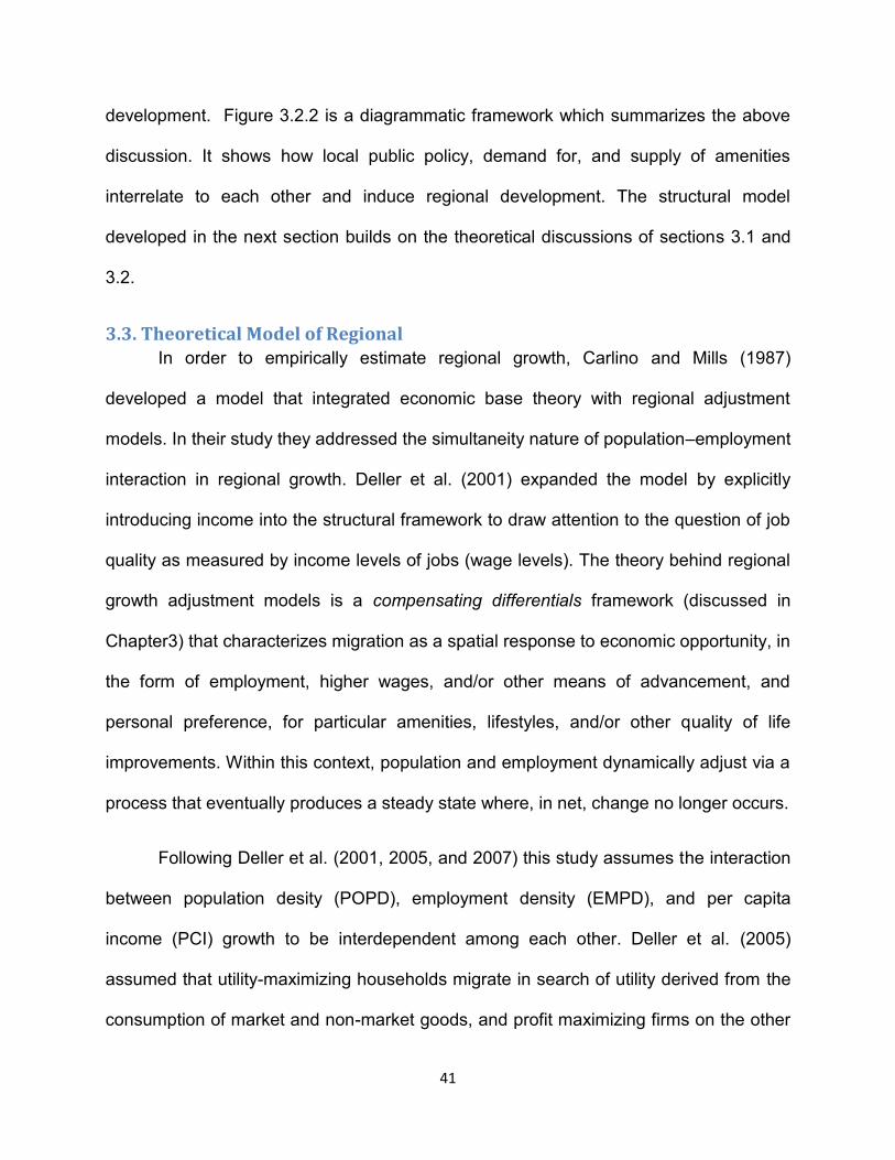
41

development. Figure 3.2.2 is a diagrammatic framework which summarizes the above

discussion. It shows how local public policy, demand for, and supply of amenities

interrelate to each other and induce regional development. The structural model

developed in the next section builds on the theoretical discussions of sections 3.1 and

3.2.

3.3. Theoretical Model of Regional In order to empirically estimate regional growth, Carlino and Mills (1987)

developed a model that integrated economic base theory with regional adjustment

models. In their study they addressed the simultaneity nature of population–employment

interaction in regional growth. Deller et al. (2001) expanded the model by explicitly

introducing income into the structural framework to draw attention to the question of job

quality as measured by income levels of jobs (wage levels). The theory behind regional

growth adjustment models is a compensating differentials framework (discussed in

Chapter3) that characterizes migration as a spatial response to economic opportunity, in

the form of employment, higher wages, and/or other means of advancement, and

personal preference, for particular amenities, lifestyles, and/or other quality of life

improvements. Within this context, population and employment dynamically adjust via a

process that eventually produces a steady state where, in net, change no longer occurs.

Following Deller et al. (2001, 2005, and 2007) this study assumes the interaction

between population desity (POPD), employment density (EMPD), and per capita

income (PCI) growth to be interdependent among each other. Deller et al. (2005)

assumed that utility-maximizing households migrate in search of utility derived from the

consumption of market and non-market goods, and profit maximizing firms on the other

42

hand become mobile when looking for regions that have lower production costs and

higher market demand. The relationship between amenity and measures of economic

development is expressed in a three equation system of “ Jobs-People-Income” as:

(3.3.1) PAPCIEMPDfPOPD ,/,

(3.3.2) EAPCIPOPDgEMPD ,/,

(3.3.3) YAEMPDPOPDhPCI ,/,

where POPD ,

EMPD , and PCI are equilibrium levels of population density,

employment density, and per capita income, respectively; ,A is a vector of measures of

local amenity indices and their interaction; P , E ,and Y are vectors of variables

describing initial conditions and other predetermined variables that affect the equilibrium

level of population density, employment density, and per capita income at the county

level. The relations in (3.3.1), (3.3.2), and (3.3.3) are based in the interdependence of

Jobs-People-Income. A simple linear relationship between the three variables can be

expressed as:

(3.3.4) P

IPIPPPP APCIEMPDPOPD 210

(3.3.5) E

IEIEEEE APCIPOPDEMPD 210

(3.3.6) Y

IYIYYYY AEMPDPOPDPCI 210

Where α, β, π, δ are coefficients that will be estimated. Following Carlino and Mills

(1987) and Deller et al. (2001, 2005 and 2007), assuming partial adjustment to

43

equilibrium, actual population density, employment density, and per capita income are

related to their lagged values plus an adjustment to the desired equilibrium level. λP, λE,

and λY are speed adjustment coefficients to the desired level of population,

employment, and income, respectively.

(3.3.7) )( 11

tPtt POPDPOPDPOPDPOPD

(3.3.8) )( 11

tEtt EMPDEMPDEMPDEMPD

(3.3.9) )( 11

tYtt PCIPCIPCIPCI

According to McDonald (1992), the speed adjustment coefficients are expected

to be between zero and one if employment, population, and income move toward the

equilibrium level (to reflect dynamic stability), whereas negative values will exist if they

overshoot the desired level and this reflects dynamic instability5. POPDt-1, EMPDt-1, and

PCIt-1 are initial conditions of population density, employment density and per capita

income, respectively. Rearranging terms and using ∆ to represent the change in the

respective variables, we derive the following equivalent equations:

(3.3.10) ),( 11

tPtt POPDPOPDPOPDPOPDPOPD

(3.3.11) )( 11

tEtt EMPDEMPDEMPDEMPDEMPD

(3.3.12) )( 11

tYtt PCIPCIPCIPCIPCI

The level of change is a direct function of the difference between the theoretical

equilibrium level and the observed level at the beginning of the period times the

5 Boarnet (1994) discusses the conditions and implications for speed adjustment coefficients below zero.

44

adjustment coefficient. The greater the distance observed or initial levels are from

equilibrium the greater the level of growth to the equilibrium level. In practice, the

theoretical equilibrium levels are not observable but can be solved from equations

(3.3.11)-(3.312).

(3.3.13) ),(1

11

tt

P

t POPDPOPDPOPDPOPD

(3.3.14) )(1

11

tt

E

t EMPDEMPDEMPDEMPD

(3.3.15) )(1

11

tt

Y

t PCIPCIPCIPCI

Substituting (3.3.13), (3.3.14), and (3.3.15) into equations (3.3.1), (3.3.2), and (3.3.3),

and rearranging terms yields the following equations (assuming linear relationship of the

endogenous variables)

(3.3.16)

,

11

13

1211210

P

IPIPtP

tPtP

Y

P

E

PP

P

APOPD

PCIEMPDPCIEMPDPOPD

(3.3.17)

E

IEIEtE

tEtEE

Y

E

P

E

E

AEMPD

PCIPOPDPCIPOPDEMPD

13

1211210

11

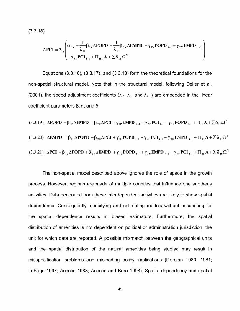
45

(3.3.18)

Y

IYIIYtY

tYtYY

P

Y

E

Y

Y

APCI

EMPDPOPDEMPDPOPDPCI

13

1211210

11

Equations (3.3.16), (3.3.17), and (3.3.18) form the theoretical foundations for the

non-spatial structural model. Note that in the structural model, following Deller et al.

(2001), the speed adjustment coefficients (λP,, λE,, and λY ) are embedded in the linear

coefficient parameters β, , and δ.

Y

IYIYtYtYtYYY

E

IEIEtEtEtEEE

P

IPIPtPtPtPPP

APCIEMPDPOPDEMPDPOPDPCI

AEMPDPCIPOPDPCIPOPDEMPD

APOPDPCIEMPDPCIEMPDPOPD

13121121

13121121

13121121

)21.3.3(

)20.3.3(

)19.3.3(

The non-spatial model described above ignores the role of space in the growth

process. However, regions are made of multiple counties that influence one another’s

activities. Data generated from these interdependent activities are likely to show spatial

dependence. Consequently, specifying and estimating models without accounting for

the spatial dependence results in biased estimators. Furthermore, the spatial

distribution of amenities is not dependent on political or administration jurisdiction, the

unit for which data are reported. A possible mismatch between the geographical units

and the spatial distribution of the natural amenities being studied may result in

misspecification problems and misleading policy implications (Doreian 1980, 1981;

LeSage 1997; Anselin 1988; Anselin and Bera 1998). Spatial dependency and spatial

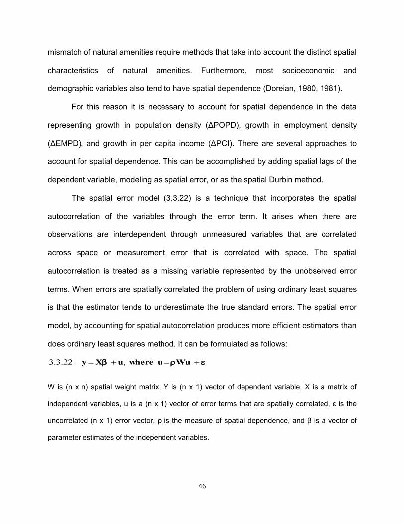
46

mismatch of natural amenities require methods that take into account the distinct spatial

characteristics of natural amenities. Furthermore, most socioeconomic and

demographic variables also tend to have spatial dependence (Doreian, 1980, 1981).

For this reason it is necessary to account for spatial dependence in the data

representing growth in population density (ΔPOPD), growth in employment density

(ΔEMPD), and growth in per capita income (ΔPCI). There are several approaches to

account for spatial dependence. This can be accomplished by adding spatial lags of the

dependent variable, modeling as spatial error, or as the spatial Durbin method.

The spatial error model (3.3.22) is a technique that incorporates the spatial

autocorrelation of the variables through the error term. It arises when there are

observations are interdependent through unmeasured variables that are correlated

across space or measurement error that is correlated with space. The spatial

autocorrelation is treated as a missing variable represented by the unobserved error

terms. When errors are spatially correlated the problem of using ordinary least squares

is that the estimator tends to underestimate the true standard errors. The spatial error

model, by accounting for spatial autocorrelation produces more efficient estimators than

does ordinary least squares method. It can be formulated as follows:

WuuwhereuXy ,22.3.3

W is (n x n) spatial weight matrix, Y is (n x 1) vector of dependent variable, X is a matrix of

independent variables, u is a (n x 1) vector of error terms that are spatially correlated, ε is the

uncorrelated (n x 1) error vector, ρ is the measure of spatial dependence, and β is a vector of

parameter estimates of the independent variables.

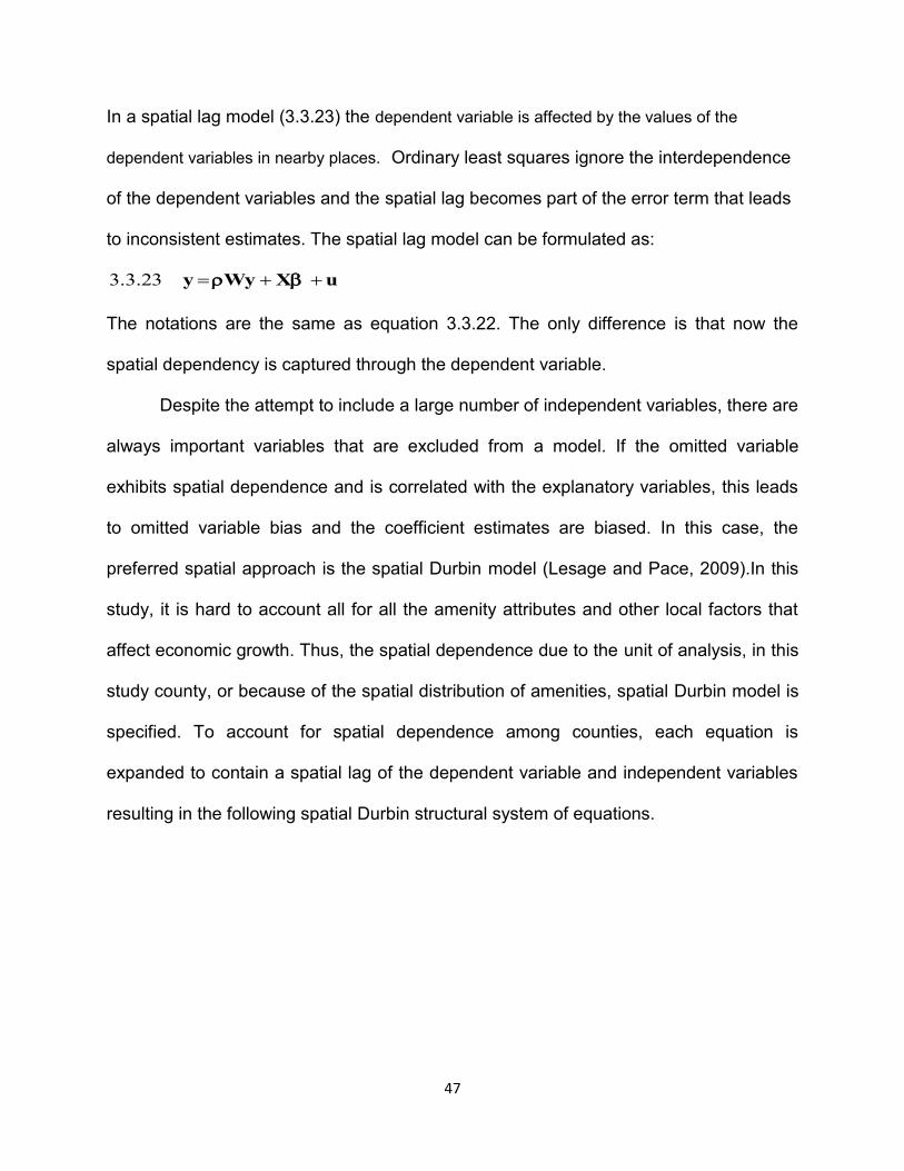
47

In a spatial lag model (3.3.23) the dependent variable is affected by the values of the

dependent variables in nearby places. Ordinary least squares ignore the interdependence

of the dependent variables and the spatial lag becomes part of the error term that leads

to inconsistent estimates. The spatial lag model can be formulated as:

uXWyy 23.3.3

The notations are the same as equation 3.3.22. The only difference is that now the

spatial dependency is captured through the dependent variable.

Despite the attempt to include a large number of independent variables, there are

always important variables that are excluded from a model. If the omitted variable

exhibits spatial dependence and is correlated with the explanatory variables, this leads

to omitted variable bias and the coefficient estimates are biased. In this case, the

preferred spatial approach is the spatial Durbin model (Lesage and Pace, 2009).In this

study, it is hard to account all for all the amenity attributes and other local factors that

affect economic growth. Thus, the spatial dependence due to the unit of analysis, in this

study county, or because of the spatial distribution of amenities, spatial Durbin model is

specified. To account for spatial dependence among counties, each equation is

expanded to contain a spatial lag of the dependent variable and independent variables

resulting in the following spatial Durbin structural system of equations.

48

Y

IYIYtYtY

tYYYY

IEIEtEtE

tEEEE

P

IPIPtPtP

tPPPP

WIAWIPCIWIEMPDWI

POPDWIPOPDWIEMPDWIPCIWPCI

WIAWIEMPDWIPCIWI

POPDWIPOPDWIPCIWIEMPDWEMPD

WIAWIPOPDWIPCIWI

EMPDWIEMPDWIPCIWIPOPDWPOPD

)()()()(

)()()()26.3.3(

)()()()(

)()()()25.3.3(

)()()()(

)()()()24.3.3(

1312

11321

1312

11321

1312

11321

W is an n by n spatial weight matrix. I is an identity and the rest notations are the same

as in the nonspatial model.

49

CHAPTER 4: EMPIRICAL MODELS AND DATA DESCRIPTION

4.1. Introduction

In Chapter 3, a theoretical model was developed to serve as a base for the

empirical model. The theoretical model reflects the interdependence of household

residential choices and firm location decisions. This interdependence is influenced by

the demand for and supply of amenities. The models outlined above and summarized in

(3.3.19.-3.3.21.) and (3.3.24.-3.3.26) are estimated using nonmetro county-level data for

the whole US and Northeast Region of the U.S. for the 1980-2005 period. Even though

the focus of this study is the Northeast Region, the study will use both datasets. The

national dataset will be used in the non-spatial empirical estimation of the model with

amenity slope shifters for the Northeast region. In section 4.1 the non-spatial model is

followed by the specification of three equations. In section 4.2 the spatial model is

described and in section 4.3 the description of data is presented.

4.2. Non-Spatial Model

An empirical model with the set of equations 4.2.1.- 4.2.3. will be estimated using

data from the 2,256 nonmetro counties of the 48 lower states of the United States for

the time period 1980 –2005. This will be followed by separate estimations for the 148

non-metro counties to assess the impact of amenities in the rural northeast region. The

econometric relationships of the regional growth indicators and amenity measures can

be specified for the non-spatial model as:

50

E

E

iEiE

tEtEtEEEE

P

P

iPiP

tPtPtPPPP

Y

Y

iYiY

tYtYtYYYY

A

EMPDPCIPOPDPCIPOPDEMPD

A

POPDPCIEMPDPCIEMPDPOPD

A

PCIEMPDPOPDEMPDPOPDPCI

13121121

13121121

13141321

)3.2.4(

)2.2.4(

)1.2.4(

YEP and ,, are the residuals of the change in population, employment, and per capita

income equations, respectively. The remaining notations are the same as described in

Chapter 3. This model, which builds on Carlino and Mills (1987) and Deller (2001),

captures growth dynamics of population, employment, and per capita income within a

region. The model hypothesizes no spillover effects in population, employment, and per

capita income among various regions. Within the framework just described above,

growth in population, employment, and per capita income are characterized as pushing

one another toward equilibrium values in the growth process, meaning that the system

is expected to register upfront a particular pattern of feedback among the three growth

variables.

The main objective of the study is to assess the role of amenities in the regional

economic growth process. Natural amenities and outdoor recreational facilities are

assumed to have a positive effect on changes in population density and employment

density, and negative effect on per capita income. Furthermore, the role of proximity of

natural amenities to the demand markets and accessibility to the supply of natural

amenities is tested. In most amenity related studies, the role of proximity and

accessibility is not recognized or totally ignored. This study contends that the availability

51

of high amenity levels alone can only create the opportunity, but to effectively promote

development, it must be complemented by other factors that can exploit the amenities

and create a comparative advantage. For example, two counties with more or less

similar amenities could follow a different development process due to differences in

infrastructure, local policies, and level of urbanization. Therefore, amenities are only one

factor, and to have effective development in rural areas requires a mix of different

factors.

This study attempts to account for proximity and accessibility by extending the

Deller (2001) model. The model is extended by introducing interaction terms to capture

the combined effect of natural and built amenities with proximity to metropolitan areas

(adjacency) and accessibility (Interstate highway density). In addition to these general

descriptions of the uniqueness of the model of this study, the equations in the model are

specified in detail in the following sections. In the empirical estimation, each equation in

the model is first specified and estimated with amenity slope shifters for the northeast6

using ordinary least squares method. This is followed by the estimation of the whole

model as a system of equations using three stage least squares with and without

augmenting the interaction terms described above.

4.2.1. Growth in Per capita Income Equation (LPCI)

Growth in per capita income is measured as the percentage change of per capita

income from 1980 to 2005. The growth in per capita income (LPCI) equation is specified

as a function of the endogenous variables of growth in population density (LPOPD) and 6 Each amenity variable is multiplied by a dummy variable that identifies the Northeast region. The

amenity variables will be multiplied by (I + NE). I is an identity and NE is a dummy that equals 1 for counties in the Northeast region and 0 otherwise. These slope shifters will test whether the natural and built amenities in the Northeast region have different impacts than in the rest of rural America.

52

employment density (LEMPD), the initial condition of per capita income in 1980 (PCI80),

measures of amenities and a vector of control variables. Equation 4.2.4 forms the base

equation in the model. This equation is expanded to include the interaction of natural

amenity (NAMTY) with highway density and adjacency to metro areas to form a proxy

for proximity of natural amenities to demand markets (NAMTYADJ) and accessibility of

natural amenities (NAMTYHWD).

ySRVMFGNRSD

UNEMPREDUPCTAXMHVWINRECWATRECHAMTY

LANDRECNAMTYPOPDPCILEMPDLPOPDLPCI

161514

13121110987

65804803210)4.2.4(

Growth in per capita income (LPCI) is expected to be negatively influenced by

growth in population density (LPOPD) and positively influenced by growth in

employment density (LEMPD). The opposite effects of growth in population (–) and

growth in employment (+) in the per capita income equation are related to the difference

between supply and demand-induced growth. Growth in population increases the labor

supply and reduces the wage rate, while growth in employment increases the demand

for labor and increases the wage rate. However, if the change in population is mainly

due to retirees or other relatively wealthy migrants (relative to the existing population)

then the prevailing wage rate may not be affected. If the retirees are wealthy enough,

they might positively affect per capita income.7 The initial condition variable reflects the

dynamics of income convergence or divergence in the region.

The measures of amenities used in the equation reflect the natural (physical and

climatic) and recreational attributes of a county. They are Natural Resource Amenities

7 Change in per capita income is a function of change in total income and population. If the change in total

income is greater than the change in population, then we can have a positive effect, the opposite when it is less than it, and no effect when both are equal.

53

(NAMTY), Historical and Cultural Amenities (HAMTY), and outdoor recreational facilities

(land-based, water–based, and winter-based, i.e., LANDREC, WATREC, and WINREC,

respectively). In the expanded equation, the role of proximity to demand markets and

accessibility of the supply of amenities is captured by two interaction terms (NAMTYADJ

and NAMTYHWD) as discussed in detail in section 4.3. According to Roback (1982 and

1988), amenities are expected to have a negative effect on per capita income because

households are willing to accept lower wages in high amenity areas. However, this

assumption is being challenged by Wu and Mishra (2008) and the findings of Deller et

al.(2008). Wu and Mishra (2008) argue that, “because amenities attract human capital,

which in turn attracts firms, locations with superior amenities tend to have a higher

demand for labor and thus higher wage rates” (p.98). Deller (2008) also found a positive

relationship between amenities and income. It seems that the direct effect is negative

and the indirect effect is positive. If this is the case, then, the net effect of amenities on

income depends on the elasticity of the direct and indirect effects.

The other control variables included in the model reflect fiscal, human capital,

market structure and economic geography for the year 1980. Per capita tax (PCTAX) is

included as a control variable to capture the negative effect of tax on change in per

capita income. The percent of 25 years and older county population with bachelor’s

degree or higher (EDU) is used as a proxy for human capital growth and is expected to

positively affect income. The local market structure variables included in the model are

the percentage earnings in natural resource dependent sector8 (NRSD) earnings in

manufacturing (MFG), and service sector (SRV). The unemployment rate (UNEMPR) is

8 In this study, percentage earnings in natural resource dependent sector (NRSD) is defined as all

earnings in farms, agricultural services, forestry, and fishing, and mining.

54

included to account for the labor market condition of the area. The urban influence code

(UIFC)9, developed by USDA Economic Research Service (1993) is used as a proxy for

the economic geography of a county. The code classifies a county based on its

population size and proximity to large urban centers. This index measures adjacency to

metro areas, and takes the lowest value (one) for metro counties with at least one

million people and the highest value (12) for counties that are the most isolated. This

index is expected to negatively affect per capita income.

4.2.2. Growth in Population Density Equation (LPOPD)

Growth in per population density is measured as the percentage change of total

population in county i from 1980 to 2005. As shown in equation 4.2.5, the growth in

population density equation is specified as a function of the initial population density

(POPD80), growth in per capita income (LPCI), growth in employment density (LEMPD),

initial per capita income (PCI80), amenity measures, and their interaction terms. A

number of exogenous variables that are hypothesized to affect household utility and

also explain temporal changes in population growth are also included. Equation 4.2.5

forms the base equation in the model. This equation is expanded to include the

interaction of natural amenity (NAMTY) with highway density and adjacency to metro

areas to form a proxy for proximity of natural amenities to demand markets

(NAMTYADJ) and accessibility of natural amenities (NAMTYHWD). All the variables

9 The urban influence codes are: 1= Large-in a metro area with at least 1 million residents or more; 2 =

Small-in a metro area with fewer than 1 million residents; 3 = adjacent to a large metro area which contains a city with at least 10,000 residents; 4 = adjacent to a large metro area that does not have a city with at least 10,000 residents; 5 = adjacent to a small metro area which contains a city with at least 10,000 residents; 6 = adjacent to a small metro area that does not have a city with at least 10,000 residents; 7 = not adjacent to a metro and contains a city with 10,000 residents; 8 = not adjacent to a metro and contains a town with 2500 – 9,999 residents; 9 = not adjacent to a metro and does not contain a town with at least 2500 residents.

55

take the 1980 values to avoid simultaneity and to help in isolating the direction of

causation.

PUIFCMFGNRSD

UNEMPRDLGEXPPCTAXMHVWINRECWATREC

HAMTYLANDRECNAMTYPOPDPCILEMPDLPCILPOPD

161514

1312111098

765804803210)5.2.4(

Growth in population density (LPOPD) is expected to be positively influenced by

change in employment density (LEMPD) and change in per capita income (LPCI). The

higher is the demand for labor as reflected by an increase in employment, the higher will

be the number of migrants who move to take advantage of the higher job opportunity.

An increase in income in an area indicates a movement towards a higher economic

status. This attracts new immigrants. Following past studies (Treyz et al.. 1993 and

Roback, 1983), a positive relationship is expected between growth in population density

(LPOPD) and growth in per capita income (LPCI). The inclusion of the initial population

level (POPD80) will capture the dynamics of population convergence or divergence in

the region.

All the amenity variables discussed in sections 4.2.1. and 4.3. are expected to

positively affect growth in population density (LPOPD) by attracting new migrants to the

area and discouraging long-term residents from leaving the region. The fiscal factors

included in the model are the direct general local government expenditures per capita

(DGLEXP) and the per capita tax rate. A high public expenditure per capita could

indicate the quantity and quality of public services provided by the local government.

Higher government spending in terms of education, health services and other basic

community services may encourage in-migration. But the higher public expenditure

depends on the tax revenue the local government can collect. Households are assumed

56

to be more attracted to counties with relatively lower levels of per capita local taxes

(PCTAX). Therefore, a higher local tax rate is expected to discourage population

growth.

The local market structure variables included in the model are the percentage

earnings in the natural resource dependent sector (NRSD) and earnings in

manufacturing (MFG). Another local characteristic that may affect population density is

the median housing value (MHV). Though it is difficult a priori to conclude on the

relationship between housing value and population growth, it may be argued that lower

housing prices may encourage population growth (though higher population growth may

increase the demand for housing and increase the price as well). The unemployment

rate (UNEMPR) is included to account for the labor market condition of the area. A

higher unemployment rate may reflect a lack of employment opportunities or a

depressed local economy. The urban influence code is included to account for the role

played by agglomeration and isolation on change in population. Areas that are close to

large urban centers are more likely to have greater population increases than those that

are more remote. Since this index takes the lowest value (one) for metro counties with

at least one million people and the highest value (12) for counties that are the most

isolated. It is expected to have a negative effect on growth in population density.

4.2.3. Growth in Employment Density Equation (LEMP)

Growth in employment density is measured as the percentage change of total

employment in county i from 1980 to 2005. Equation 4.2.6 describes the specification of

growth in employment density (LEMPD) equation. It is a function of the growth in per

capita income (LPCI), growth in population density (LPOPD), the initial employment

density (EMPD80), initial per capita income (PCI80), and amenity measures (Ai) as

57

shown in equation 4.2.6. Growth in employment (LEMP) is expected to be positively

influenced by growth in population (LPOPD) and per capita income (LPCI). As

population and income increases, there is more demand for goods and services which

translates into more demand for labor by firms. The initial level of employment density

will capture the divergence and convergence in employment density in the region. The

initial level of per capita income (PCI80) will serve as a proxy to the relative initial

strength of the economy.

The same amenity variables discussed in Sections 4.2.1. and 4.2.2 are included

in this equation (4.2.6). Power (1996) argues that some firms may view the

attractiveness of the region as a place to work and do business. In addition, these areas

may attract or have high quality labor forces which are willing to work in the region for

lower wages. Thus, the amenity variables are expected to have a positive effect on

change in employment density by attracting new firms to the area and increasing the

demand for labor.

PUIFCSRVMFG

NRSDCREATIVEDLGEXPPCPTAXEDUWINRECWATREC

HAMTYLANDRECNAMTYEMPDPCILPOPDLPCILEMPD

171615

141312111098

765804803210)6.2.4(

In addition, a number of exogenous variables are also included to determine

growth in employment density (LEMPD). Direct local government expenditures

(DLGEXP) are included to capture the role of public local services in attracting business

to the region. Per capita property tax (PCPTAX) is included to account for business

costs imposed by local governments. Taxes reduce business profits and adversely

affect the ability of firms to demand for more labor. Since firms may be attracted to a

58

region with a relatively higher-quality labor force, the percent of the population with

bachelor’s degree or higher (EDU) is included to measure this effect. The percentage of

workers considered as part of the creative class (CREATIVE) is included to account for

the creativeness of an area in generating new ideas and jobs. The market structure

variables included in the model are the percentage of earnings in the natural resource

dependent sector (NRSD), the percentage of earnings in manufacturing (MFG), and

percentage earnings in services (SRV). The urban influence code is also included to

account for the role of agglomeration and isolation in growth in employment density

(LEMPD). Areas that are close to large urban centers are more likely to have greater

demands for goods and services, high quality of public infrastructure, and low cost of

information (due to formal and informal networks) compared to those that are more

remote. This condition creates a conducive environment for the growth of firms. Since

this index takes the lowest value (one) for metro counties with at least one million

people and the highest value (12) for counties that are the most isolated, it is expected

to have a negative effect on change in employment density (LEMPD).

4.3. Spatial Model In the amenity and regional growth literature, the role of spillover effects is

recognized in very few studies. The spatial model developed below is different from

Deller et al. (2005) and Nzaku and Bukenya (2005). Both studies extended the Deller et

al. (2001) model by incorporating a spatial component to capture the role of spatial

interdependence among the variables. Nzaku and Bukenya (2005) included a spatial

lag of the dependent variable in each equation. Deller et al. (2005) estimated a spatial

error model to account for the spatial interdependence in the error terms. These

59

extensions moved the empirical models of amenities and regional growth models one

step forward but the estimation of these empirical models of both studies didn’t account

for the spatial distribution of amenities. The empirical model developed in this study will

account for the spatial dependency and mismatch of amenities by adapting the spatial

Durbin method.

Each of the three equations in the model are specified as a function of

endogenous dependent variables (LPOPD,LEMPD, and LPCI), Amenities (A), other

exogenous variables (X), and spatially weighted dependent variables(WLPOPD,

WLEMPD, and WLPCI), amenities (WA), and independent variables (WX). The amenity

(A) and exogenous variables (x) in each equation in the spatial Durbin model are the

same as the variables in the equations (4.2.4 - 4.2.6) of the nonspaitial model.

Y

Y

IYIY

YYY

E

E

IEIE

EEE

P

P

IPIP

PPP

uWIAWI

PCIYWILEMPDWILPOPDWIWPCILPCI

uWIAWI

EMPDWILPCIYWILPOPDWIWLEMPDLEMPD

uWIAWI

POPDWILPCIWILEMPWIWLPOPDLPOPD

)()(

)()()(*)3.3.4(

)()(

)()()(*)2.3.4(

)()(

)()()(*)1.3.4(

80321

80221

80121

(rho) is a measure of strength of the spatial dependence and is the coefficient of the

spatial lag of the dependent variable in each of the equations. W is 299 x 299 (n x n)

row–standardized weight matrix constructed from the nearest neighbors (the number of

the nearest neighbors differs from study to study). I is an identity. The residuals of the

growth in population, employment, and per capita income equations are ,,, YEP uanduu

respectively. The remaining notations are the same as defined in the non-spatial model.

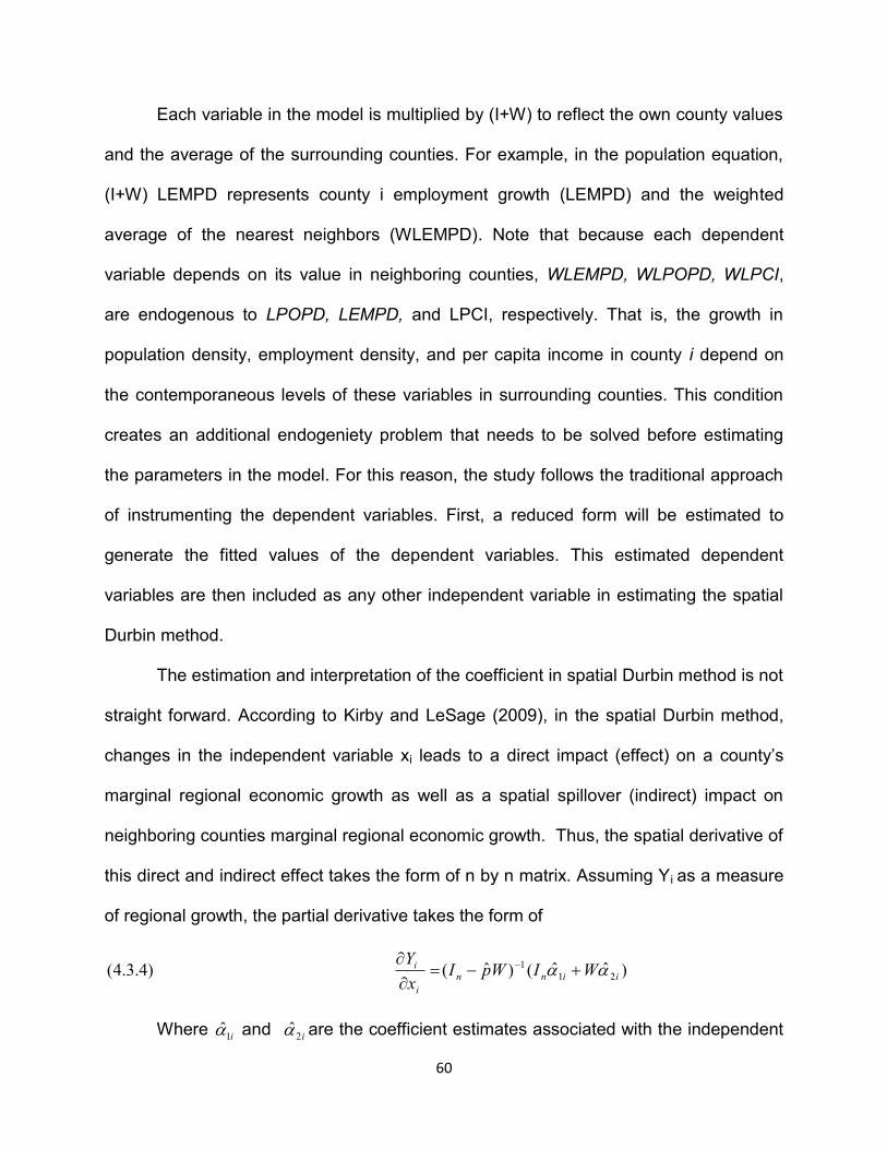
60

Each variable in the model is multiplied by (I+W) to reflect the own county values

and the average of the surrounding counties. For example, in the population equation,

(I+W) LEMPD represents county i employment growth (LEMPD) and the weighted

average of the nearest neighbors (WLEMPD). Note that because each dependent

variable depends on its value in neighboring counties, WLEMPD, WLPOPD, WLPCI,

are endogenous to LPOPD, LEMPD, and LPCI, respectively. That is, the growth in

population density, employment density, and per capita income in county i depend on

the contemporaneous levels of these variables in surrounding counties. This condition

creates an additional endogeniety problem that needs to be solved before estimating

the parameters in the model. For this reason, the study follows the traditional approach

of instrumenting the dependent variables. First, a reduced form will be estimated to

generate the fitted values of the dependent variables. This estimated dependent

variables are then included as any other independent variable in estimating the spatial

Durbin method.

The estimation and interpretation of the coefficient in spatial Durbin method is not

straight forward. According to Kirby and LeSage (2009), in the spatial Durbin method,

changes in the independent variable xi leads to a direct impact (effect) on a county’s

marginal regional economic growth as well as a spatial spillover (indirect) impact on

neighboring counties marginal regional economic growth. Thus, the spatial derivative of

this direct and indirect effect takes the form of n by n matrix. Assuming Yi as a measure

of regional growth, the partial derivative takes the form of

)ˆˆ()ˆ()4.3.4( 21

1

iinn

i

i WIWpIx

Y

Where i1̂ and i2̂ are the coefficient estimates associated with the independent

61

variable xi and Wxi respectively. The coefficient p̂ measures the strength of the spatial

dependence. LeSage and Pace (2009) developed a scalar summary measure for the n

by n partial derivative of direct and indirect effects arising from the change in the

independent variable. This study will follow their approach and present the direct,

indirect, and total effects alongside the estimated coefficients of the model in chapter 5.

Beyond this general description of the relationship of the variables, the expected sign of

the relationship of the variables remains the same as in the nonspatial model.

4.4. Types and Sources of Data

In order to estimate the empirical model, relevant data, including the endogenous

variables, initial conditions of the endogenous variables, amenities and their interaction,

and local county characteristics (fiscal, human capital, market structure, and economic

geography) are collected for the 2,256 counties of the U.S. However, the focus of the

study is the Northeast region which has 299 counties of which 148 are non-metro

counties.

The data used in the study reflects the 1980-2005 period. All the dependent

variables are expressed as growth rates of the period 1980-2005. All the independent

variables take the 1980 values to avoid simultaneity and to help in isolating the direction

of causation. With the exception of the amenity variables, the rest of the variables are

expressed as location quotients or the ratio of the local value to the national mean. This

transformation ensures that each observation is pegged to the US economic system as

a whole (Carruthers , Hollar , Mulligan, (2006). The result is unit free and enables direct

comparison of growth in population density, employment density, and per capita income

at equilibrium. The secondary data used in the study are drawn from several sources.

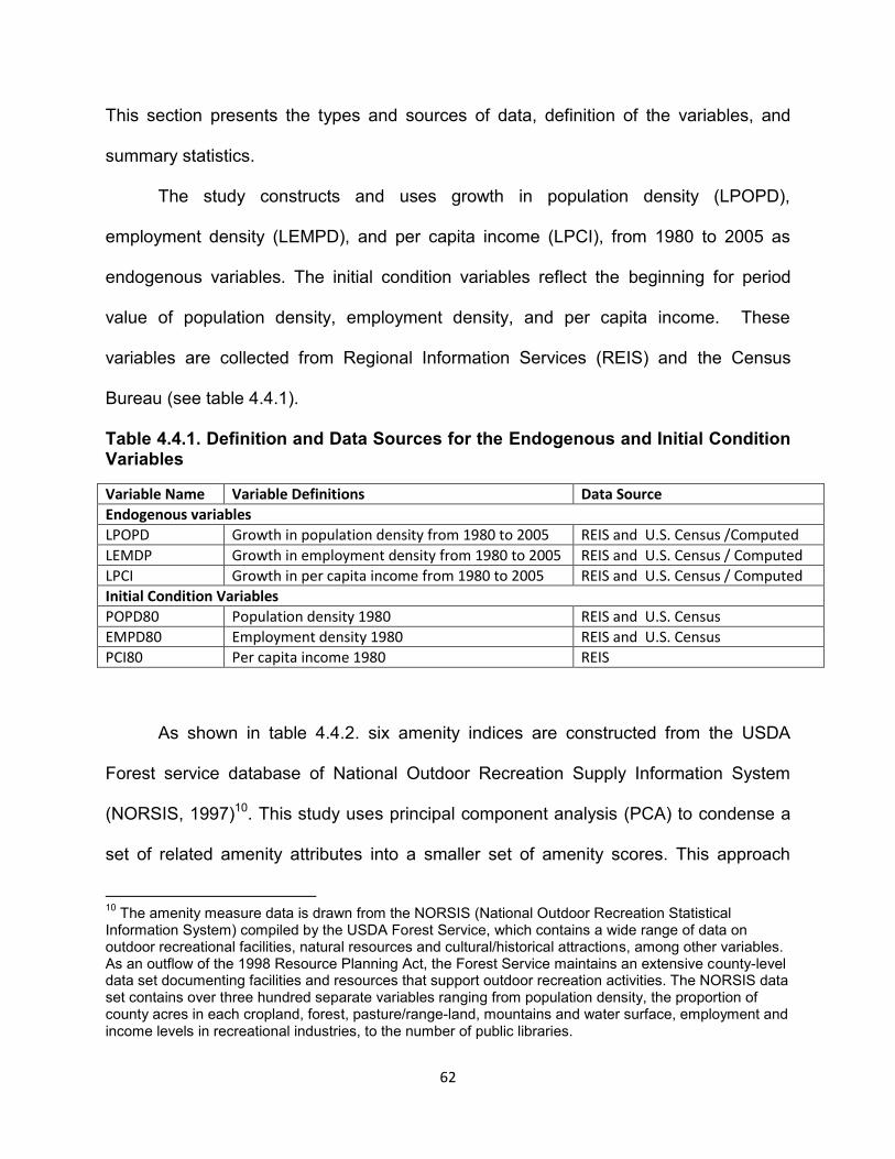
62

This section presents the types and sources of data, definition of the variables, and

summary statistics.

The study constructs and uses growth in population density (LPOPD),

employment density (LEMPD), and per capita income (LPCI), from 1980 to 2005 as

endogenous variables. The initial condition variables reflect the beginning for period

value of population density, employment density, and per capita income. These

variables are collected from Regional Information Services (REIS) and the Census

Bureau (see table 4.4.1).

Table 4.4.1. Definition and Data Sources for the Endogenous and Initial Condition Variables

Variable Name Variable Definitions Data Source

Endogenous variables

LPOPD Growth in population density from 1980 to 2005 REIS and U.S. Census /Computed

LEMDP Growth in employment density from 1980 to 2005 REIS and U.S. Census / Computed

LPCI Growth in per capita income from 1980 to 2005 REIS and U.S. Census / Computed

Initial Condition Variables

POPD80 Population density 1980 REIS and U.S. Census

EMPD80 Employment density 1980 REIS and U.S. Census

PCI80 Per capita income 1980 REIS

As shown in table 4.4.2. six amenity indices are constructed from the USDA

Forest service database of National Outdoor Recreation Supply Information System

(NORSIS, 1997)10. This study uses principal component analysis (PCA) to condense a

set of related amenity attributes into a smaller set of amenity scores. This approach

10

The amenity measure data is drawn from the NORSIS (National Outdoor Recreation Statistical Information System) compiled by the USDA Forest Service, which contains a wide range of data on outdoor recreational facilities, natural resources and cultural/historical attractions, among other variables. As an outflow of the 1998 Resource Planning Act, the Forest Service maintains an extensive county-level data set documenting facilities and resources that support outdoor recreation activities. The NORSIS data set contains over three hundred separate variables ranging from population density, the proportion of county acres in each cropland, forest, pasture/range-land, mountains and water surface, employment and income levels in recreational industries, to the number of public libraries.

63

allows measuring and evaluating multiple natural amenities into distinct groupings.

Following the National Outdoor Recreation Supply Information System (NORSIS, 1997),

Goe and Green (2002), and Deller (2001, 2005, 2007), the groupings included in this

study are Natural Resource Amenities, Historical and cultural amenitiesHistorical and

Cultural Amenities, and built-in outdoor recreational facilities (land-based, water-based,

and winter-based). More than 35 county level attributes are used to construct these six

amenity indices. Even though, the

Table 4.4.2. Definition and Data Sources for Natural Amenities and Outdoor Recreational Facilities

Variable Definition Data Source

CLIMATE Climate Index NORSIS 1997 /Computed

NAMIX Natural Resource Amenity Index NORSIS 1997/ Computed

LANDREC Land-based outdoor recreational facilities Index NORSIS 1997/ Computed

WATREC Water-based outdoor recreational facilities Index NORSIS 1997/ Computed

WINREC Winter-based outdoor recreational facilities Index NORSIS 1997/ Computed

HAMTY Historical and cultural Amenity Index NORSIS 1997/ Computed

NAMTYADJ Adjacent to metro times natural amenity Index Computed

NAMTYHWD Highway density times natural amenity Index Computed

standard convention in principal component analysis is to retain components with

eigenvalues greater than one, the study retains only the first component. This is done to

increase the degree of freedom in the estimation process. In most cases, the first

component is the best summary of the entire data set and accounts for most of the

variance. Tables 4.4.3-4.4.8 show the eigenvector loadings of the first component of

each of the amenity indices. Furthermore, GIS maps that show the spatial distribution of

each of the amenity indices in the Northeast region are included in Appendix 1.

The climate index is constructed from 5 climatic variables (Table 4.4.3). The first

component explains 48.7% of the variability of the data. With the exception of average

64

January sunshine, all of the rest make a significant contribution in the final index. As

shown in Figure 4.1 (Appendix 1), the spatial distribution of the climate index is not

uniform. Counties in the South and Southeastern part of the region scored high while

counties found in the heavy snow and cold area in the Northern New England scored

low. In the study area, the five counties with the highest score are found in Maryland

(Somerset, St. Mary’s, Wicomico, Talbot, and Dorchester).

Table 4.4.3. Climate Index

Variable Name Eigenvector

Average January Temperature 0.545

Average Precipitation 0.529

Average July Temperature 0.476

Average Humidity 0.432

Average January Sunshine 0.099

Total Variability explained 48.70%

The natural resource (landscape) amenity index (NAMIX) is constructed from 10

local physical attributes (Table 4.4.4). The first component explains 35.76% of the

variability of the data. The major contributors for the final index are AWA total white

water river miles, NRI total river miles (outstanding value), Bailey acres of mountains,

NRI forest of acres, and USDA-FS forest and grassland acres. Attributes such as

availability of coastal area, and FWS refuge acres open for recreation do not contribute

to the final natural amenity index. As shown in Figure 4.2 (in the appendix), the spatial

distribution of the natural resource amenity index is not uniform. Counties in the

Northern part of the New England states and counties in Eastern and Southeastern part

of West Virginia scored high in the index. Overall, counties in Maine, Aroostook,

Piscataquis, Somerset, Washington, and Penobscot scored the highest in the index.

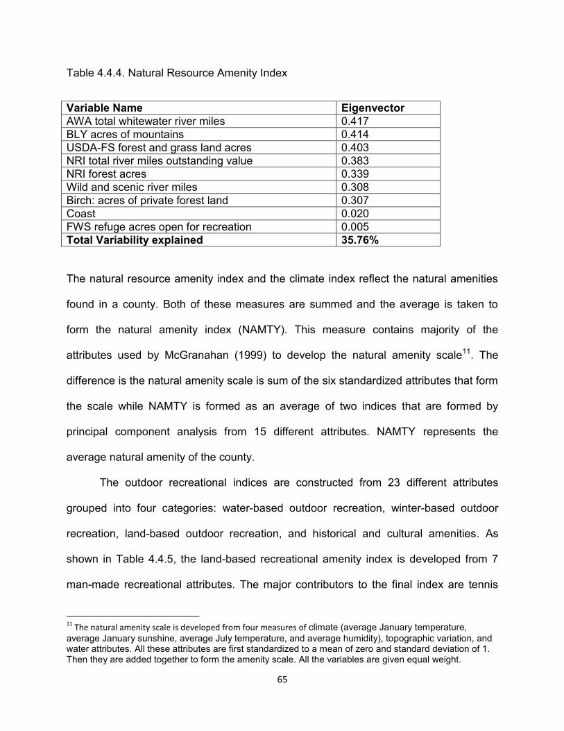
65

Table 4.4.4. Natural Resource Amenity Index


AWA total whitewater river miles 0.417

BLY acres of mountains 0.414

USDA-FS forest and grass land acres 0.403

NRI total river miles outstanding value 0.383

NRI forest acres 0.339

Wild and scenic river miles 0.308

Birch: acres of private forest land 0.307

Coast 0.020

FWS refuge acres open for recreation 0.005


The natural resource amenity index and the climate index reflect the natural amenities

found in a county. Both of these measures are summed and the average is taken to

form the natural amenity index (NAMTY). This measure contains majority of the

attributes used by McGranahan (1999) to develop the natural amenity scale11. The

difference is the natural amenity scale is sum of the six standardized attributes that form

the scale while NAMTY is formed as an average of two indices that are formed by

principal component analysis from 15 different attributes. NAMTY represents the

average natural amenity of the county.

The outdoor recreational indices are constructed from 23 different attributes

grouped into four categories: water-based outdoor recreation, winter-based outdoor

recreation, land-based outdoor recreation, and historical and cultural amenities. As

shown in Table 4.4.5, the land-based recreational amenity index is developed from 7

man-made recreational attributes. The major contributors to the final index are tennis

11

The natural amenity scale is developed from four measures of climate (average January temperature,

average January sunshine, average July temperature, and average humidity), topographic variation, and water attributes. All these attributes are first standardized to a mean of zero and standard deviation of 1. Then they are added together to form the amenity scale. All the variables are given equal weight.

66

courts, parks and recreational departments, golf courses, and playgrounds and

recreational centers. The final index explains 56.4% of the variability in the data. As

shown in Figure 4.3 in the Appendix , Westchester, Suffolk, and Nassau counties in the

state of New York, Middlesex in Massachusetts, and Montgomery in Pennsylvania

scored high in the index.

Table 4.4.5. Land-based Recreational Amenity Index


ABI number of private and public tennis courts 0.444

ABI number of parks and recreation departments 0.438

ABI number of private and public golf courses 0.421

ABI number of playgrounds and recreational centers 0.409

ABI number of organized camps 0.394

ABI number of private and public swimming pools 0.317

ABI number of hunting, fishing preserves, lodges, and clubs 0.103


Table 4.4.6 shows the four attributes that form the water-based recreational

amenity index. The first component of the water-based outdoor recreational amenity

index explains 31.04% of the variability of the data. The major contributors for the final

index are attributes related to fishing and marinas. Counties like Ocean in New Jersey,

Suffolk in New York, and Anne Arundel in Maryland scored the highest in this index.

The spatial distribution of water-based recreational amenities is shown in Figure 4.4 in

the Appendix .

Table 4.4.6. Water-based Recreational Amenity Index


ABI number of fish camps, private and public fish lakes, piers and ponds 0.663

ABI number of marinas 0.640

ABI number of canoe outfitters, rental firms, raft trip firms 0.316

ABI number of diving instructors, tours, and snorkel outfitters 0.224


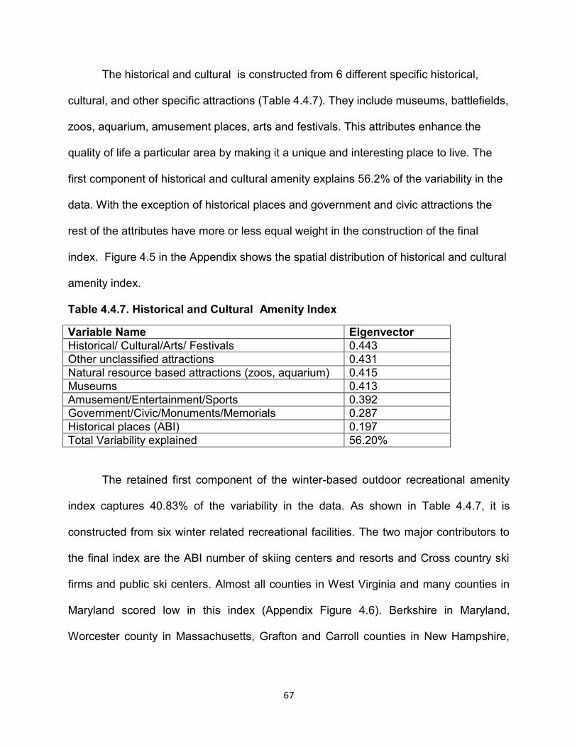
67

The historical and cultural is constructed from 6 different specific historical,

cultural, and other specific attractions (Table 4.4.7). They include museums, battlefields,

zoos, aquarium, amusement places, arts and festivals. This attributes enhance the

quality of life a particular area by making it a unique and interesting place to live. The

first component of historical and cultural amenity explains 56.2% of the variability in the

data. With the exception of historical places and government and civic attractions the

rest of the attributes have more or less equal weight in the construction of the final

index. Figure 4.5 in the Appendix shows the spatial distribution of historical and cultural

amenity index.

Table 4.4.7. Historical and Cultural Amenity Index


Historical/ Cultural/Arts/ Festivals 0.443

Other unclassified attractions 0.431

Natural resource based attractions (zoos, aquarium) 0.415

Museums 0.413

Amusement/Entertainment/Sports 0.392

Government/Civic/Monuments/Memorials 0.287

Historical places (ABI) 0.197


The retained first component of the winter-based outdoor recreational amenity

index captures 40.83% of the variability in the data. As shown in Table 4.4.7, it is

constructed from six winter related recreational facilities. The two major contributors to

the final index are the ABI number of skiing centers and resorts and Cross country ski

firms and public ski centers. Almost all counties in West Virginia and many counties in

Maryland scored low in this index (Appendix Figure 4.6). Berkshire in Maryland,

Worcester county in Massachusetts, Grafton and Carroll counties in New Hampshire,

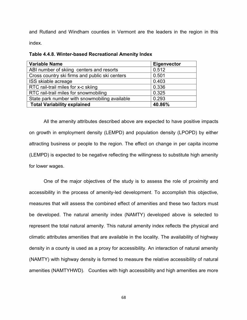
68

and Rutland and Windham counties in Vermont are the leaders in the region in this

index.

Table 4.4.8. Winter-based Recreational Amenity Index


ABI number of skiing centers and resorts 0.512

Cross country ski firms and public ski centers 0.501

ISS skiable acreage 0.403

RTC rail-trail miles for x-c skiing 0.336

RTC rail-trail miles for snowmobiling 0.325

State park number with snowmobiling available 0.293


All the amenity attributes described above are expected to have positive impacts

on growth in employment density (LEMPD) and population density (LPOPD) by either

attracting business or people to the region. The effect on change in per capita income

(LEMPD) is expected to be negative reflecting the willingness to substitute high amenity

for lower wages.

One of the major objectives of the study is to assess the role of proximity and

accessibility in the process of amenity-led development. To accomplish this objective,

measures that will assess the combined effect of amenities and these two factors must

be developed. The natural amenity index (NAMTY) developed above is selected to

represent the total natural amenity. This natural amenity index reflects the physical and

climatic attributes amenities that are available in the locality. The availability of highway

density in a county is used as a proxy for accessibility. An interaction of natural amenity

(NAMTY) with highway density is formed to measure the relative accessibility of natural

amenities (NAMTYHWD). Counties with high accessibility and high amenities are more

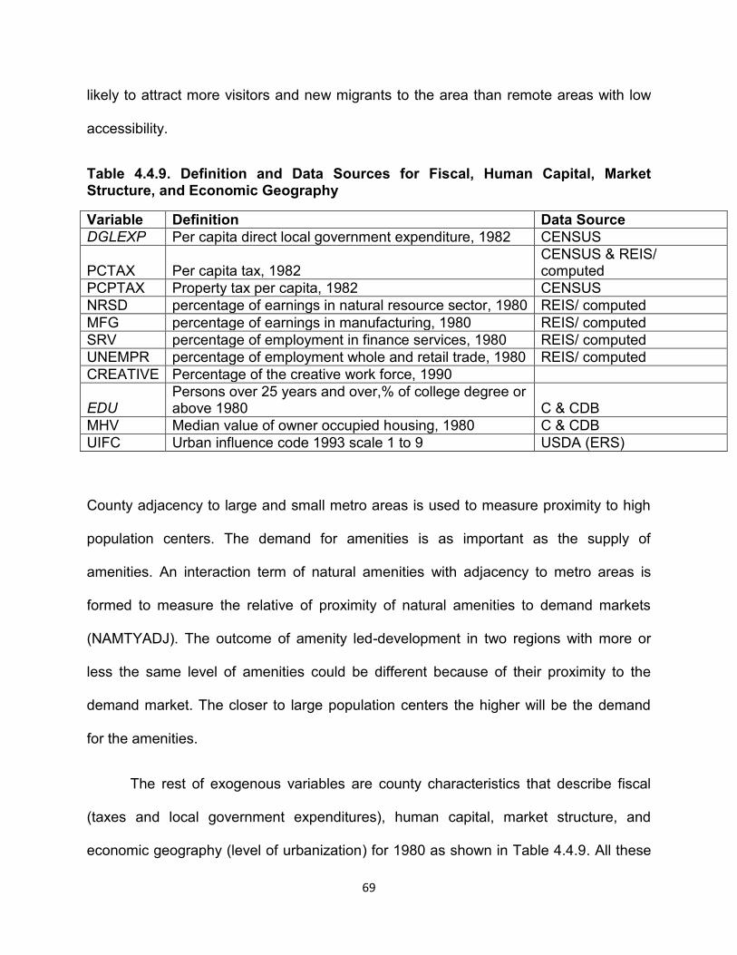
69

likely to attract more visitors and new migrants to the area than remote areas with low

accessibility.

Table 4.4.9. Definition and Data Sources for Fiscal, Human Capital, Market Structure, and Economic Geography

Variable Definition Data Source

DGLEXP Per capita direct local government expenditure, 1982 CENSUS

PCTAX Per capita tax, 1982 CENSUS & REIS/ computed

PCPTAX Property tax per capita, 1982 CENSUS

NRSD percentage of earnings in natural resource sector, 1980 REIS/ computed

MFG percentage of earnings in manufacturing, 1980 REIS/ computed

SRV percentage of employment in finance services, 1980 REIS/ computed

UNEMPR percentage of employment whole and retail trade, 1980 REIS/ computed

CREATIVE Percentage of the creative work force, 1990

EDU Persons over 25 years and over,% of college degree or above 1980 C & CDB

MHV Median value of owner occupied housing, 1980 C & CDB

UIFC Urban influence code 1993 scale 1 to 9 USDA (ERS)

County adjacency to large and small metro areas is used to measure proximity to high

population centers. The demand for amenities is as important as the supply of

amenities. An interaction term of natural amenities with adjacency to metro areas is

formed to measure the relative of proximity of natural amenities to demand markets

(NAMTYADJ). The outcome of amenity led-development in two regions with more or

less the same level of amenities could be different because of their proximity to the

demand market. The closer to large population centers the higher will be the demand

for the amenities.

The rest of exogenous variables are county characteristics that describe fiscal

(taxes and local government expenditures), human capital, market structure, and

economic geography (level of urbanization) for 1980 as shown in Table 4.4.9. All these

70

variables are collected from Bureau of Economic Analysis (BEA-REIS), City and County

Data Book (C & CDB), the Census Bureau, and the Economic Research Services

(ERS) of USDA. The data reflect the year 1980 and are at the county level. The

summary descriptive statistics of the variables in the two models are presented in Table

4.4.10.

Table 4.4.10 Summary Descriptive Statistics

Variable Mean Median

Maximum Minimum Std. Dev. LEMPD 0.782 0.698 3.353 -2.248 0.639

LPOPD 0.409 0.315 4.197 -2.784 0.844

LPCI 1.007 1.010 1.240 0.682 0.098

EMPD80 8.354 1.583 325.164 0.033 29.469

PCI80 0.887 0.861 1.542 0.508 0.185

POPD80 8.992 1.776 495.356 0.045 35.550

NAMTY 0.259 0.056 8.884 -0.715 0.875

HAMTY -0.065 -0.360 10.132 -0.489 0.912

LANDREC 1.181 0.217 15.664 -0.899 2.635

WATREC 0.271 -0.219 11.961 -0.421 1.456

WINREC 1.236 0.409 13.589 -0.506 2.429

NAMTYADJ 0.104 0.000 4.862 -0.715 0.460

NAMTYHWD 69.833 43.082 2095.672 -1652.800 408.444

DLGEXP 0.864 0.768 2.044 0.436 0.304

PCTAX 0.922 0.891 3.671 0.156 0.479

PCPTAX 1.028 1.015 4.405 0.196 0.594

NRSD 1.740 0.651 20.511 -1.157 3.079

MFG 1.130 1.113 3.222 0.015 0.586

SRV 0.861 0.837 2.268 0.000 0.343

UNEMPR 1.201 1.169 2.938 0.292 0.394

CREATIVE 0.176 0.168 0.397 0.071 0.059

EDU 0.835 0.735 2.642 0.272 0.367

MHV 0.870 0.803 2.059 0.336 0.276

UIFC93 4.058 3.000 9.000 1.000 2.738

71

CHAPTER 5: EMPIRICAL RESULTS AND ANALYSIS

5.1. Introduction

The main focus of this chapter is to empirically estimate the relationship between

natural and built amenities and regional economic growth. Growth in population density,

employment density, and per capita income will be used as indicators of regional

economic growth. Amenity indices representing natural amenities (climate and natural

physical attributes), historical and cultural amenities, land, water, and winter based

recreational amenities will be used as measures of local amenities.

This chapter consists of two major sections and four subsections within each

section. Section one presents the results of the nonspatial model and section two

discusses the estimated results of the spatial Durbin model. At the end of each section,

a summary of major findings is presented.

5.2. Findings and Analysis of Non-Spatial Regional Growth Model

The nonspatial model (equations 4.26 through 4.30) estimates the relationship

between the endogenous variables of growth in population density, employment

density, and per capita income, with five amenity indices and a set of exogenous

variables specific to each equation. In estimating the effects of amenities in the process

of economic growth in the northeast region, the study follows a variety of Deller and

Lledo (2007) slope shifters approach. A set of amenity slope shifters are introduced

which allow each of the amenity variable coefficients to differ for the northeast region.

This allows us to see whether amenities in the rural northeast behave in different ways

than for the rest of rural America. When examining the slope coefficients we are looking

72

for the overall statistical significances, signs, and magnitude of the coefficients. If the

slope shifter coefficient is statistically significant, then it can be concluded that rural

northeast behaved differently than the rest of the country in terms of amenities. If the

coefficient has the same sign as the base variable, it indicates that the effects are

stronger in rural northeast than the rest of rural America. If it is of opposite sign it means

the effects are weaker.

First, each equation is estimated using all amenity and exogenous variables by

the ordinary least square method. Amenity slope shifters for the northeast region are

included in the estimation to see if there is a difference between the national and

regional impacts. The US nonmetro data set is used to exploit the degrees of freedom

of a large sample size. The first column of Tables 5.2.1-5.2.3 present the results of the

ordinary least squares model with slope shifters (OLS_US_NE). This specification is

similar to the reduced form estimation of Deller et al. (2001), Deller and Lledo (2007),

and Nazku and Bukenya( 2005). Column 2 (3SLS_US_NE 1) of each of the three tables

presents the base results from the estimation of system of equations with amenity slope

shifters for the region using US nonmetro data set. Three stage least squares is

preferred over two stage least squares because of the high correlation of the residuals

of the population and employment equations. Column 3 (3SLS_US_NE 2) presents the

tests for the role of proximity of natural amenities (NAMTYADJ) to the demand market

and accessibility of the supply of natural amenities (NAMTYHWD). Finally, column four

(3SLS_NE) presents estimation results using data for the nonmetro northeast region.

5.2.1. Growth of Population Density (LPOPD)

Table 5.2.1 shows the results of the population growth equation estimated using

ordinary least square (OLS_US_NE) with amenity slope shifters for the northeast region

73

(column 1) and three estimation results using three stage least squares. The overall fit

of the estimation was good with adjusted R2 ranging from 0.398- 0.771which is

consistent with similar studies (for example, Deller and Lledo (2007) reported R2

ranging from 0.575 - 0.769 in their reduced form estimation of amenities and population

growth).

The first three rows of the table show the results of the endogenous dependent

variables. As shown in the table, employment growth has a positive and significant

effect on population growth in 3SLS_US_NE_1 and 3SLS_US_NE 2 and no effect in

3SLS_NE (probably due to small sample size). These results are consistent with labor

demand theories of regional development. Employment growth indicates the availability

of high labor demand in the area. People migrate to take advantage of the job

opportunities. This result implies that people follow jobs. In all the equations, per capita

income growth has no effect on population growth in the region. Thus, in this study,

there is no evidence that indicates people migrate to capture higher income in the

northeast region.

One of the key assumptions used in developing our model was that growth is

dependent on initial conditions. In all the results, the initial level of population density

was highly significant and negative. This result is consistent with past studies (Deller et

al. 2001 and Hailu and Brown 2007). It implies that areas with initial high population

densities are growing slower compared to areas with low initial population densities.

This gives supports to the convergence of population density.

The results from the OLS_US_NE and 3SLS_US_NE 1 provide evidence of

significant differences between the northeast region and the rest of the country in terms

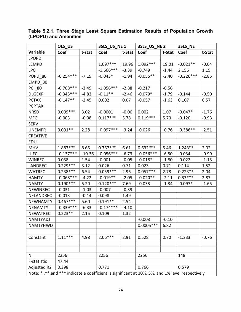
74

Table 5.2.1. Three Stage Least Square Estimation Results of Population Growth (LPOPD) and Amenities

Variable

OLS_US 3SLS_US_NE 1 3SLS_US_NE 2 3SLS_NE

Coef t-stat Coef t-Stat Coef t-Stat Coef t-Stat

LPOPD

LEMPD 1.097*** 19.96 1.092*** 19.01 -0.021** -0.04

LPCI -1.666*** -3.39 -0.749 -1.44 2.156 1.15

POPD_80 -0.254*** -7.19 -0.043* -1.94 -0.055** -2.40 -0.226*** -2.85

EMPD_80

PCI_80 -0.708*** -3.49 -1.056*** -2.88 -0.217 -0.56

DLGEXP -0.345*** -4.83 -0.11** -2.46 -0.079* -1.79 -0.144 -0.50

PCTAX -0.147** -2.45 0.002 0.07 -0.057 -1.63 0.107 0.57

PCPTAX

NRSD 0.009*** 3.02 -0.0001 -0.06 0.002 1.07 -0.047* -1.76

MFG -0.003 -0.08 0.117*** 5.78 0.119*** 5.70 -0.120 -0.93

SERV

UNEMPR 0.091** 2.28 -0.097*** -3.24 -0.026 -0.76 -0.386** -2.51

CREATIVE

EDU

MHV 1.887*** 8.65 0.767*** 6.61 0.632*** 5.46 1.243** 2.02

UIFC -0.137*** -10.36 -0.056*** -6.73 -0.056*** -6.50 -0.034 -0.99

WINREC 0.038 1.54 -0.001 -0.05 -0.018* -1.80 -0.022 -1.13

LANDREC 0.229*** 3.12 0.026 0.71 0.023 0.71 0.114 1.52

WATREC 0.238*** 6.54 0.059*** 2.96 0.057*** 2.78 0.223** 2.04

HAMTY -0.068*** -4.22 -0.019** -2.05 -0.020** -2.11 0.33*** 2.87

NAMTY 0.190*** 5.20 0.120*** 7.69 -0.033 -1.34 -0.097* -1.65

NEWINREC -0.031 -1.03 -0.007 -0.39

NELANDREC -0.013 -0.14 0.098 1.49

NEWHAMTY 0.467*** 5.60 0.191** 2.54

NENAMTY -0.339*** -6.33 -0.174*** -4.10

NEWATREC 0.223** 2.15 0.109 1.32

NAMTYADJ -0.003 -0.10

NAMTYHWD 0.0005*** 6.82

Constant 1.11*** 4.98 2.06*** 2.91 0.528 0.70 -1.333 -0.76

N 2256 2256 2256 148

F-statistic 47.44

Adjusted R2 0.398 0.771 0.766 0.579

Note: * ,**,and *** indicate a coefficient is significant at 10%, 5%, and 1% level respectively

75

of the role of amenities. The results of the reduced form show that with the exception of

winter based recreational amenities (WINREC), all the base amenity variables are

statistically significant. The coefficients of natural amenities (NAMTY), land based

recreational amenities (LANDREC), and water based recreational amenities

(WATREC) are positive and significant while historical and cultural amenities (HAMTY)

is negative.

Looking at the amenity slope shifters, only three were significant. NAMTY was

negative and significant while HAMTY and WATREC were positive and significant.

LANDREC which has a strong and positive effect in the rest of the country does not play

any role in the region. The positive coefficient of WATREC indicates that the effect of

this amenity is stronger in the northeast than in the rural America. The coefficient of

HAMTY which is negative and weak in the base is positive and strong for the region.

The direct opposite of this coefficient is the coefficient of NAMTY. It is positive and

strong for the country but negative for the region. This is not a surprising finding. Even

though, the Northeast region has its own natural qualities, the climate condition (snow

and cold) is not as good as the southern part of the country. Furthermore, most of the

non-metro parts of the region are found in the Appalachian mountains of West Virginia

and Pennsylvania. This lack of natural appeal could be one of the reasons for the

negative relationship.

The relatively strong and positive coefficient of HAMTY indicates that those

counties in the region with historical and cultural sites, zoos, museums, amusement,

sports, and other entertainment places, can greatly enhance the quality of life of the

area which can draw new migrants and visitors. The same is true for counties with

76

greater number of WATREC that can supply local residents and tourists with a variety of

water based entertainments. These results indicate that conclusions based on

generalization of national level analysis could be misleading. Different regions have

different natural and built amenities which could have region specific effects. Generally,

amenity indicators were hypothesized to play a positive role in population growth. But as

discussed above some of the measures are negative.

The results from 3SLS_US_NE 2 in Table 5.2.1 presents the test result of the

role of proximity to the amenity demand market and accessibility to supply of amenity in

the population and amenity relationship. The two coefficients of interest are the

interaction terms AMTYADJ and AMTYHWD. AMTYADJ is the interaction of NAMTY

with adjacency12 to metro area which is used as proxy to measure the effect of proximity

to the amenity demand market. AMTYHWD is the interaction of NAMTY with highway

density which is used as proxy to show the relative accessibility of the supply of

amenities. NAMTYHWD is positive and significant indicating accessibility to the supply

of amenities matters. Counties which complement their natural appeal by investing in

infrastructure could have a comparative advantage over others with similar natural

appeals. This supports the hypothesis that places with higher accessibility and higher

natural amenities attract in-migrants which boost the population. But the small

magnitude of the coefficient of NAMTYHWD implies that a huge investment in

infrastructure is needed to get the feasible effect. The coefficient of NAMTYADY is not

significant indicating proximity to large population centers does not play a significant

role.

12

Adjacency to metro area is defined based on urban influence code of 1993 developed by the USDA. Urban influence codes 3, 4, 5, 6 are defined as counties adjacent to big and small metro areas.

77

3SLS_NE presents the region specific 3SLS estimation results for the effects of

amenities. Caution is needed in analyzing these results. The sample size is relatively

small as the northeast has only 148 nonmetro counties. The estimation can suffer from

small sample size. But, nevertheless the results are consistent with the estimation using

slope shifters. WINREC and LANDREC do not play any role. NAMTY, as in the slope

shifters, is negative and significant. HAMTY and WATREC are positive and significant.

From all these findings, it is clear that natural amenities, historical and cultural

amenities, and water based recreational facilities play a role in shaping the population

growth of the northeast region. But in interpreting these results an understanding of how

these variables are constructed is required. For example, WATREC is positive and

significant. This implies, holding everything equal, rural regions that have access to a

variety of water based recreation resources also have higher level of population growth.

This does not mean that all water based recreational facilities have equal impacts. In

the construction of WATREC, places that have marinas and fishing related activities are

weighted higher than the others and have a greater impact.

Several control variables which potentially affect population growth are included

in all the estimation processes. Three out of 7 variables are significant and have the

expected signs for the northeast region. Unemployment rate and earnings in natural

resource dependent industries are negative while the median value of owner occupied

housing is positive. But at the national level, with the exception of natural resource

dependency variable, all are significant. The most important is the role of economic

geography (UIFC). This measure of agglomeration and remoteness is significant and

negative consistent with regional development theories. Both, lack of agglomeration and

78

remoteness greatly reduce the attractiveness of place as destination for in-migrants but

encourage out-migration of population. This suggests that even if amenities in two

places are the same, people prefer places that are less remote. One unexpected result

is the negative coefficient of the direct local government expenditure (DLGEXP).The

effects of public expenditure depends on the type and magnitude of that expenditure.

Public investments in education, health care, highways, and crime prevention are more

likely to enhance quality of life as opposed to expenditures directed to welfare

payments. Given that many of the rural counties of the northeast are found in

Appalachia and depend on federal assistance programs, the negative relationship is not

surprising. The coefficient of UNEMPR shows negative sign and is also statistically

significant in the region specific estimation. This implies counties with higher

unemployment rates also have lower population growth rates. However, at the national

level, UNEMPR is positively associated with population growth.

5.2.2. Employment Growth Equation (LEMPD)

Similar to the population equation, the estimated employment growth equation

explained in the range of 32% -75.7% of the variations (Table 5.2.2 column 1-4) in the

dependent variable. As shown in the table, in national and region specific estimation,

population growth has a positive and significant effect on employment growth. This

result implies that jobs follow people. High population growth is one measure of the

supply of labor. For any given demand for labor, if the supply of labor increases the

wage rate falls. Firms will demand more of this cheap labor. Per capita income has a

negative effect in the national level estimation and no effect in the regional estimation.

The initial level of employment density is negative and significant at the national level.

This shows counties with high employment density in the 1980s have had slower

79

Table 5.2.2. Three Stage Least Square Estimation Results of Employment Growth and Amenities (LEMPD)

Variable

OLS_US_NE 3SLS_US_NE 1 3SLS_US_NE 2 3SLS_NE

Coef Coef Coef

t-Stat Coef t-Stat Coef

t-Stat

LPOPD 0.704*** 14.49 0.679*** 16.12 0.433*** 4.09

LEMPD

LPCI -1.146*** -2.72 -0.788* -1.89 0.095 0.11

POPD_80

EMPD_80 -0.24*** -6.51 0.012 0.43 -0.001 -0.04 -0.038 -1.14

PCI_80 -0.765*** -5.80 -1.266*** -4.45 -1.093*** -3.85

DLGEXP -0.194*** -3.47 0.005 0.15 -0.005 -0.16 -0.365*** -3.04

PCTAX

PCPTAX -0.05* -1.86 0.072*** 2.70 0.066** 2.48 0.107 1.51

NRSD 0.004* 1.76 -0.003* -1.84 -0.003* -1.89 -0.025** -2.21

MFG -0.024 -0.95 -0.075*** -3.68 -0.087*** -4.50 -0.109* -1.75

SERV -0.007 -0.13 0.107*** 2.61 0.054 1.33 0.344*** 3.38

UNEMPR

CREATIVE 9.521*** 10.97 2.248** 3.27 2.271*** 3.65 0.366 0.25

EDU -0.082 -0.77 -0.074 -1.49 -0.076* -1.72 0.141 0.68

MHV

UIFC -0.063*** -6.22 0.022** 2.13 0.016* 1.68 -0.010 -0.62

WINREC 0.077*** 5.52 0.029*** 2.71 0.030*** 3.47 -0.012 -1.09

LANDREC 0.188*** 4.07 -0.0002 -0.01 -0.003 -0.11 -0.101*** -2.14

WATREC 0.151*** 5.97 0.005 0.26 0.012 0.67 0.083 1.50

HAMTY -0.032*** -2.93 0.015 1.54 0.010 1.07 -0.006 -0.10

NAMTY 0.027 1.51 -0.107*** -5.88 -0.016 -0.70 0.022 0.67

NEWINREC -0.081*** -4.67 -0.004 -0.22

NELANDREC -0.196*** -3.47 -0.093 -1.43

NEWHAMTY 0.258*** 4.80 -0.116 -1.48

NENAMTY -0.093*** -3.23 0.130*** 2.91

NEWATREC 0.121* 1.71 0.060 0.75

NAMTYADJ -0.003 -0.14

NAMTYHWD -0.0002*** -3.50

Constant 0.959*** 6.51 2.042*** 3.81 1.686 3.16 0.555 0.62

N 2256 2256 2256 148

F-statistic 45.13

Adjusted R2 0.321 0.612 0.651 0.757


80

employment growth compared to counties with low employment density. The results

support the employment convergence hypothesis. A high level of initial per capita

income is also associated with negative employment growth.

The results from the OLS_US_NE in table 5.2.2 provide further evidence of

significant difference between the northeast region and the rest of the country in terms

of the role of amenities. The results of the reduced form show that with the exception of

NAMTY, all the base amenity variables are significant. The coefficients of LANDREC,

WATREC, AND WINREC are positive and significant while (HAMTY) is negative.

Looking at the amenity slope shifters, all are significant in the reduced form.

NAMTY which is not significant in the base variable model is significant and negative.

This is consistent with the impact of NAMTY on population growth. In both cases, the

northeast not only differs from the rest of the country but also its NAMTY depresses

growth. As in the population growth case, both HAMTY and WATREC are positive and

significant for the region. The positive coefficient of WATREC indicates the effect of this

amenity is stronger in the northeast than the rest of rural America. The coefficient of

HAMTY which is negative and weak in the base is again positive and strong for the

region. The direct opposite of this is the coefficients of LANDREC and WINREC. They

are positive for the country but negative for the region.

In the 3SLS_US_NE1 case, only WINREC and NAMTY from the base variables and the

slope shifter of NAMTY are significant. Moving from a simple OLS estimation to the full

information estimation of three stage least square almost doubled the R2 (32.1%to

61.2%) but reduced the magnitude of the amenity coefficients. The NAMTY coefficient

81

which is consistently negative for the region turned positive. WINREC was positive in

both OLS and 3SLS_US_NE1 results.

3SLS_US_NE 2 presents the test result of the role of proximity to the amenity

demand market and accessibility to supply of amenity in the employment and amenity

relationship. NAMTYHWD which is positive for the population equation turned negative

and significant indicating accessibility to the supply of amenities depresses employment

growth. In both cases the magnitude of the coefficients is very small (0.0005 for

population growth and -0.0002 for employment growth) which greatly reduces its

importance as a determining factor in the regional economic growth process. Similar to

the population growth result, the coefficient of NAMTYADY is not significant indicating

proximity to large population centers does not play a role in employment growth.

In the region specific estimation (3SLS_NE) only LANDREC is significant and in

line with the OLS slope shifter case which is negative. (It is hard to explain the

consistent negative relationship between land based recreational facilities and

employment growth within the region). All the rest of the amenity variables are

insignificant indicating no role of amenities in employment growth. But considering the

simultaneity between population growth and employment growth, the indirect effect of

amenities (WATREC and HAMTY positive and NAMTY negative effect on population

growth, table 5.2.1 column 2) at the regional level cannot be ignored. One possible

reason for this finding could be related to the argument and finding of Henderson and

McDaniel (2005). They argued that the relationship between natural amenities and

employment growth varies by industry and natural amenity type. The impact of

amenities is clearer for the service and retail sectors than others. If this is the case then,

82

our aggregate employment growth measure is not capturing this effect or the

contribution of the service and retail sectors to the overall employment growth. Either

way, there is a need for sector specific studies to reach a sound conclusion on the

relationship.

The performance of the control variables is not as expected. With the exception

of the percentage of creative class and economic structure indicators, the rest of the

control variables switched signs from one to the other. As expected, the coefficient of

the percentage of creative class is positive and significant in all the national level

analyses. This implies counties with a higher percentage of this group will have higher

growth in employment. The economic structure indicator variables are significant at the

regional level. Percentage earnings in natural resource dependent industries (NRSD)

and manufacturing (MFG) are negative and significant. This is a logical relationship as

the importance of these two sectors has greatly decreased in the last quarter of the last

century. The positive and significant coefficient of the percentage earnings in the

service sector (SRV) shows the growing dominance of the sector in creating

employment during the period. Again as in the population equation, DLGEXP is

negative and significant. Henderson and McDaniel (2005) also found a similar negative

relation between manufacturing sector employment growth and local government

expenditures. Contrary to theoretical expectations, the coefficient of property tax per

capita (PCPTAX) is positive and significant which implies the higher the property tax the

higher will be the employment growth. There is no logical explanation for this

relationship. Property taxes are part of business costs and there is no practical

explanation that can support this finding. The percentage of adults with college degree

83

(EDU) does not seem to play a role in regional or national employment growth. In most

cases, the coefficient either has the unexpected sign or is not significant.

5.2.3. Change in Per Capita Income Equation (LPCI)

The overall fit of the per capita income growth equation, as shown Table 5.2.3,

ranges from 35.5% - 50.9%. This is almost double the OLS reduced form estimation of

Deller and Lledo (2007) for rural Appalachia. But given the difference in time period (10

vs. 25 years), estimation technique (OLS vs. 3SLS), and region (Appalachia vs.

northeast US) such differences could be justifiable.

At the national level, there is a strong positive interdependence between LPOPD and

LPCI. This indicates the growth in population, which also a proxy to growth of the supply

of labor, didn’t affect the wage rate. Holding labor demand and other factors constant,

the growth in labor supply is expected to lower the wage rate which is the major

component of personal income. But during end of the last century, the US economy

experienced a very low unemployment rate, which suggests that the demand for labor

has been high. If the change in the demand for labor is higher than the supply of labor

and if other sources of income (investment income) have been growing fast, it is not

surprising to see strong positive relationship between growth in population and income.

This relationship is reversed at the regional level. LPOPD is inversely related to LPCI in

the Northeast region. One reason could be counties with higher population growth in

the region have been experiencing lower per capita income growth. Average county

income with a growing population may decline if income growth does not keep pace

with population growth. As hypothesized, high employment growth is associated with

high income growth in the region.

The initial level of per capita income (PCI80) is consistently negatively related to

84

Table 5.2.3. Estimation Results of Income Growth and Amenities, 1980-2005

Variable

OLS_US_NE 3SLS_US_NE 1 3SLS_US_NE 2 3SLS_NE

Coef t-stat Coef t-stat Coef t-stat Coef t-stat

LPOPD 0.038** 2.56 0.056*** 3.64 -0.153** -2.08

LEMPD -0.035 -1.60 -0.054** -2.37 0.201** 2.16

LPCI

POPD_80 0.018*** 5.16 0.018*** 3.91 0.019*** 4.17

EMPD_80

PCI_80 -0.762*** -19.79 -0.76*** -33.32 -0.774*** -32.28 -0.480*** -4.30

DLGEXP

PCTAX 0.040*** 3.16 0.045*** 9.19 0.049*** 9.80 0.052** 2.27

PCPTAX

NRSD -0.002* -1.93 -0.002*** -5.36 -0.002*** -5.75 -0.005* -1.74

MFG 0.010* 1.92 0.057*** 6.65 0.055*** 6.45 -0.013 -0.80

SERV 0.053*** 4.45 0.007 1.56 0.004 0.75 -0.0002 -0.01

UNEMPR -0.042*** -7.28 -0.040*** -8.36 -0.042*** -8.36 -0.099*** -2.59

CREATIVE

EDU 0.011 0.75 0.015 1.10 0.013 0.96 0.012 0.29

MHV 0.150*** 7.53 0.113*** 5.42 0.102*** 4.94 0.231*** 2.73

UIFC

WINREC 0.008*** 2.64 0.008*** 3.73 0.010*** 5.08 0.001 0.36

LANDREC -0.002 -0.27 -0.005 -0.58 -0.003 -0.45 -0.002 -0.12

WATREC 0.007** 2.38 0.004 0.96 0.005 1.14 0.046*** 3.13

HAMTY 0.004*** 3.17 0.006*** 2.86 0.005*** 2.63 0.008 0.48

NAMTY -0.013*** -3.18 -0.019*** -5.32 -0.012** -2.37 0.006 0.83

NEWINREC 0.001 0.15 0.0003 0.07

NELANDREC -0.002 -0.15 -0.006 -0.40

NEWHAMTY -0.017 -1.60 -0.026 -1.64

NENAMTY 0.014*** 2.63 0.023** 2.43

NEWATREC 0.046*** 3.56 0.044*** 2.61

NAMTYADJ 0.004 0.82

NAMTYHWD -0.00003* -1.82

Constant 1.413*** 47.08 1.438*** 66.66 1.469*** 64.66 1.212*** 13.16

N 2256 2256 2256 148

F-statistic 70.8

Adjusted R2 0.509 0.437 0.388 0.385


85

the growth of income. This negative and significant relationship suggests that counties

with lower income initially experienced greater income growth than counties with higher

income in the earlier period. This may suggest a trend in regional growth towards

development in rural areas (Deller et al. 2001) and supports the income convergence

argument.

The negative but weak relationship between NAMTY and income growth at the

national level lends evidence to the compensating differential argument. According to

Roback (1982 and 1988), amenities are expected to have a negative effect on per

capita income because households are willing to accept lower wages in high amenity

areas. But the slope shifter of NAMTY for the northeast is positive and significant

(almost of equal magnitude) which indicates that at the regional level NAMTY may play

some role. The base variable for WATREC and the slope shifter are both positive and

significant which suggest a strong role of WATREC in the region. This is also confirmed

by the positive and significant coefficient of the region specific estimation. HAMTY and

WINREC are positive at the national level but neither the slope shifter nor the region

specific coefficient is significant for the northeast. This positive relationship of HAMTY,

WATREC, and WINREC support the arguments of Wu and Mishra (2008) and the

findings of Deller and Leldo (2008). Wu and Mishra (2008) argue that, “because

amenities attract human capital, which in turn attracts firms, locations with superior

amenities tend to have a higher demand for labor and thus higher wage rates” (p.98).

Does this finding contradict the assumptions of Roback (1982 and 1988)? The

relationship between amenities and income is not clear cut.

Many of the amenities such as HAMTY, WATREC, and WINREC are not pure

86

natural amenities. They are built amenities which take advantage of the natural physical

attributes of the area. There can also be a direct effect which is negative and indirect

effect which is positive as suggested by Wu and Mishra (2008). If this is the case, then

the net effect of amenities on income depends on the direct and indirect effects of

income elasticity.

The 3SLS_NE 2 results of Table 5.2.3 presents the test result of the role of

proximity to the amenity demand market and accessibility to supply of amenities in the

income and amenity relationship. As in the case of employment growth NAMTYHWD is

negative and significant indicating accessibility to the supply of amenities depress

income growth. In both cases the magnitude of the coefficients is very small (-0.0002 for

employment growth and -0.00003 for income growth) which greatly reduces its

importance as a determining factor in the regional economic growth process. Similar to

the population and employment growth results, the coefficient of NAMTYADY is not

significant indicating proximity to large population centers does not play any role in

income growth.

Counties with higher level of NRSD (percentage of earning from farming,

agricultural services, and mining) are also associated with low levels of income growth.

This is true because the share of the extractive resources sector is declining in the US.

In Chapter 1 a comparison is made between Jefferson and McDowell, two counties in

West Virginia. The growth of per capita income for McDowell county which depends on

coal (extractive resource) was almost half of Jefferson county (156% and 336%

respectively). Jefferson transformed and diversified its economy and was able to record

high income growth.

87

In line with the economic theory and past studies, counties with higher

unemployment rates (UNEMPR) experienced slower income growth. The coefficient of

UNEMPR is significant and negative in all the estimated results. The unemployment

rate may be measuring the local business climate, with higher unemployment rates

indicating a less attractive place to do business. Contrary to theoretical expectations,

the percentage of adults with college degree (EDU) does not seem to play a role in

regional or national income growth. In all cases, the coefficient has the expected sign,

but it is not statistically significant.

5.2.4. Summary Findings of Non-Spatial Regional Growth Model

The main goal of the regional economic growth model is to understand and assess

the relationships between regional growth trends and natural and built amenities. For

this reason, growth in population density, employment density, and per capita income

were modeled as endogenous variables, and the role of natural and built amenities in

the regional economic growth process was examined. This section provides the major

findings of the non-spatial empirical estimation.

Natural (NAMTY) and built amenities (specifically HAMTY and WATREC) play

opposing roles in shaping the growth rate of population density for the northeast

region of the US. In addition to the amenity factors, initial population density,

dependence on the natural resource extraction sector, median value of owner

occupied housing value, and the unemployment rate are found to be

determinants of population growth during the period of 1980-2005. From all these

findings, it is clear that natural amenities, historical and cultural amenities, and

water based recreational facilities play a role in shaping the northeast region’s

population growth.

88

The role of amenities in influencing the growth in employment density at the

regional level is different from the growth of employment density at the national

level. Amenities, except for land based recreational facilities, are found to have

no role in determining employment density growth. Growth in population density,

local government expenditures per capita, percentage of earnings in the natural

resources, manufacturing, and service sectors, and percentage of the creative

class are found to be the major determinants of growth in employment density.

Water based recreational amenities are found to be the only amenity variable

that influenced the growth in per capita income in the last quarter of the 20th

century. Other factors such as growth in population and employment densities,

initial level of per capita income, earnings in the natural resource extraction

sector, median value of owner occupied housing value, per capita tax rate and

the unemployment rate are found to be determinants of population growth during

1980-2005 period.

The national data set for all metro areas is used to test for the relationship

between proximity to amenity demand markets (AMTYADJ) and accessibility to

the supply of amenities (AMTYHWD) and regional growth indicators. No

relationship is detected between the proximity to the amenity demand market and

all three measures of regional growth. The test is conducted using adjacency to

metro areas as a proxy to proximity to the amenity demand market. One of the

reasons for this finding could be the choice of proxy. Instead of adjacency,

distance from metro areas could be an alternative proxy.

There is no clear cut relationship between regional growth indicators and the

89

proxy for the supply of natural amenities (NAMTYHWD). In line with the

expectations, it is positive and significant in the population growth equation

indicating accessibility to the supply of amenities matters. But it is negative and

significant for the employment and income growth equations which indicates that

accessibility to the supply of amenities depresses regional growth. There are no

logical explanations for these two contradicting results. In all cases, the

magnitudes were very small which diminishes but does not eliminate its

significance as a major determining factor.

5.3. Findings and Analysis of Spatial Durbin Model The results of the empirical estimation in section 5.1 were based on the

assumption that there is no spatial dependence. Regular regression models are applied

that assumed that regions are independent of one another. As discussed in section 4.3,

it is not realistic to ignore space when observations are collected from regions located in

space. Ignoring the existence of spatial dependence produces estimates that are biased

and inconsistent. This section accounts for the spatial dependence by estimating the

spatial models developed in Chapters 3 and 4. The spatial Durbin model that accounts

for spillover effects by adding spatial lags for the dependent and independent variables

is used as a method of spatial analysis. By using this method, the model is expected to

capture the direct and indirect effects of amenities in the process of regional growth.

The issue of simultaneity of the regional economic growth indicators creates a

challenge in the estimation of the spatial Durbin model. The current mat lab code that is

used to estimate this model does not have the internal capability of estimating

simultaneous equations. For this reason, the study follows the traditional approach of

90

instrumenting the dependent variables. First, a reduced form is estimated to generate

the fitted values of the dependent variables. These estimated dependent variables are

then included as any other independent variable in estimating the spatial Durbin

method. Therefore, each of the three equations in the model are estimated as a function

of endogenous dependent variables (LPOPD, LEMPD, and LPCI), spatially weighted

dependent variables (WLPOPD, WLEMPD, and WLPCI), independent variables (vector

X), spatially weighted independent variables (WX).

As discussed in Chapter 4, the estimation and interpretation of the coefficients of

the spatial model are not straightforward. According to Kirby and LeSage (2009), in the

spatial Durbin method, changes in the independent variable xi lead to a direct impact

(effect) on a county’s marginal regional economic growth as well as a spatial spillover

(indirect) impact on neighboring county’s marginal regional economic growth. This

study will follow this approach and present the direct, indirect, and total effects

alongside the estimated coefficients of the model. Since the objective of the study is to

assess the spatial effects of amenities on regional economic growth, the focus of the

discussion will be on the estimated direct, indirect, and total effects not on the estimated

coefficients of the model.

The strength of the estimated spatial dependence is measured by rho. As shown

in table 5.3.1, none of the rho values for the nonmetro northeast region is statistically

significant at any level. This could be due to the estimation of rho using a small sample

size or the construction of the weight matrix. The use of nonmetro counties only in the

construction of the weight matrix eliminates all the metro counties in the region that

could have strong spatial relationships. In this case, the spillover effects of the metro

91

counties to the surrounding nonmetro counties are not captured.

One way to overcome this problem is to separately construct the weight matrix

using all counties in the region and estimate the model using the nonmetro counties.

Table 5.3.1. Estimated Value of the Spatial Dependence Statistic, Rho

Equations

Non-metro NE All counties NE

Coeff. P-level Coeff. P-level

LPOPD 0.101 0.27 0.328*** 0

LEMP 0.072 0.33 0.147* 0.09

LPCI -0.265 0.10 0.333*** 0.00

N 148 299

However, the existing available methodology which is used to estimate the spatial

Durbin model does not have this flexibility. Another option is to construct all the spatial

lags and export them to other statistical software and use nonmetro counties in the final

estimation of the model. But this also has the problem of estimating only the initial direct

and indirect effects. The additional feedback effects which are set in motion by the initial

effects are ignored. Thus, the estimated coefficient could under or overestimate the

spatial spillover effect.

In light of the above empirical estimation challenge, this study estimates both

cases. First the model is estimated using data for the whole northeast metro and

nonmetro counties and then a separate estimation is made using the subsample of only

the nonmetro counties. But the analysis of the results will depend on the full sample

size of all northeast counties. For comparison, the results of the estimation of the

nonmetro counties are attached in the appendix. The weight matrix is constructed using

the nearest eight neighboring counties.

5.3.1. Spatial Result of Growth in Population Density

Table 5.3.2. presents the results of the spatial Durban model for the growth in

92

population density equation. The statistically significant value of the spatial dependence

measure (rho) shows a strong spatial interdependence among regions. The model

explains an estimated 68.2% of the variation in the growth of population density. In

terms of magnitude, median value of owner occupied houses has the highest direct

positive effect while percentage of earnings in manufacturing exerted the greatest

impact in reducing population growth. Natural amenity (NAMTY) and historical and

cultural amenity (HAMTY) are the only two with positive spatial spillover effects.

The estimated results show that growth in employment density has a positive

direct effect on population growth. This result is similar to the result of the nonspatial

model of 5.2.1. Growth in employment density indicates an increase in labor demand.

This job opportunity attracts new in-migrants to the region which leads to growth in

population and implies people follow jobs. The direct effect of per capita income is also

positive. Contrary to the results of the nonspatial model which found no relationship,

these results suggest that people migrate to capture higher incomes. Growth in per

capita income is associated with high growth in population density. However, the

indirect effects of employment and per capita income are not significant. This indicates

the growth of employment and per capita income in surrounding counties does not have

an impact on population growth. The value of rho which is also the coefficient for growth

in population density in surrounding counties is positive and significant. This means

growth in population in surrounding counties has positive spillover effect.

Turning to the amenity variables, the direct effect of NAMTY is negative and

significant while the indirect effect is positive. This strong and positive indirect effect is

not captured by the nonspatial model. This implies that a county that lacks natural

93

Table 5.3.2. Spatial Durbin Estimation Results of Population Growth and Amenities

Model results Direct effect Indirect effect Total effect

Variable Coeffi p-level Coeff t-prob Coeffi p-level Coeff t-prob

LEMPD 0.220*** 0.03 0.209** 0.08 -0.355 0.41 -0.146 0.75

LPCI 0.936*** 0 0.960*** 0 0.748 0.48 1.707 0.14

POPD80 -0.001 0.14 -0.001 0.22 -0.003 0.14 -0.004* 0.07

DLGEXP -0.261* 0.09 -0.262 0.18 -0.038 0.95 -0.3 0.63

PCTAX 0.001 0.51 0.003 0.99 0.061 0.9 0.064 0.9

NRSD -0.018* 0.09 -0.026** 0.06 -0.242*** 0 -0.268*** 0

MFG -0.250*** 0 -0.278*** 0 -0.906** 0.01 -1.184*** 0

UNEMPR 0.047 0.35 0.035 0.77 -0.376 0.38 -0.341 0.43

MHV 1.085*** 0 1.087*** 0 0.058 0.94 1.145 0.16

UIFC 0.034** 0.04 0.031 0.1 -0.096 0.17 -0.065 0.36

LANDREC -0.075*** 0 -0.077*** 0 -0.084 0.29 -0.161** 0.05

WATREC 0.023 0.2 0.024 0.37 0.024 0.84 0.048 0.69

HAMTY 0.076** 0.01 0.087** 0.01 0.380** 0.04 0.467** 0.02

NAMTY -0.145** 0.01 -0.134** 0.02 0.357* 0.06 0.223 0.16

WINREC 0.016 0.18 0.016 0.37 -0.01 0.85 0.005 0.93

WLEMPD -0.316 0.14

WLPCI 0.186 0.39

WPOPD80 -0.002* 0.09

WDLGEXP 0.063 0.44

WPCTAX 0.041 0.45

WNRSD -0.158*** 0

WMFG -0.531** 0.01

WUNEMPR -0.272 0.18

WMHV -0.33 0.28

WUIFC -0.077* 0.06

WLANDREC -0.032** 0.27

WWATREC 0.009 0.47

WHAMTY 0.232** 0.02

WNAMTY 0.292** 0.02

WWINREC -0.012 0.37

rho 0.328*** 0

constant 0.548 0.33

R2 0.682

N 299


94

attractions of its own can still benefit from high amenities in its surrounding areas. From

the built amenities, the direct, indirect, and total effect of historical and cultural amenity

is positive and significant while the direct and total effect of land based recreational

facilities is negative. There is no theoretical justification for this negative relationship of

LANDREC with population density growth. This index is driven mainly by the availability

of parks and recreation departments, private and public tennis courts, recreational

centers, and golf courses. One possible reason for the negative relationship could be

the construction and developments of land based recreational facilities are reducing

land available for growth.

The total effect of the initial population density is negative indicating convergence

in population growth within the region. Counties with high population density in 1980

were growing slower compared to those with low population density. The direct, indirect,

and total effect of NRSD and MFG is negative and significant. Natural resource and

manufacturing dependent counties are associated with population loss. McDowell

County of West Virginia, which depends on coal (extractive resource), is a good

example. It lost 52.1% of its population during the study period. The strong positive

direct effect of median value of owner occupied suggests that Increase in population

density is high in areas where the median housing values is high like VT and NH.

5.3.2. Spatial Result of Employment Density Growth

The relatively weak statistical significance of rho in Table 5.3.3. shows a weak spatial

interdependence among regions in the estimated employment density growth equation.

The model explains an estimated 65.9% of the variation in the growth of employment

95

Table 5.3.3. Spatial Durbin Estimation Results of Employment Growth and Amenities



POPD 0.460*** 0 0.461*** 0 0.068 0.72 0.529*** 0

LPCI 0.661*** 0 0.661*** 0 -0.027 0.97 0.635 0.37

EMPD80 0.00001 0.5 0.00003 0.97 0.001 0.64 0.001 0.66

DLGEXP -0.443*** 0 -0.444*** 0 -0.033 0.93 -0.477 0.23

PCPTAX 0.328*** 0 0.330*** 0 0.118 0.74 0.448 0.23

NRSD -0.044*** 0 -0.046*** 0 -0.140*** 0 -0.185*** 0

MFG -0.322*** 0 -0.329*** 0 -0.388 0.07 -0.716*** 0

SRV 0.109 0.17 0.105 0.34 -0.271 0.46 -0.166 0.68

EDU -0.018 0.44 -0.018 0.88 -0.007 0.98 -0.025 0.94

UIFC 0.058*** 0 0.058*** 0 -0.029 0.5 0.029 0.5

LANDREC -0.025** 0.04 -0.026* 0.08 -0.049 0.25 -0.075* 0.09

WATREC -0.018 0.2 -0.019 0.38 -0.062 0.44 -0.081 0.31

HAMTY 0.025 0.19 0.029 0.32 0.216** 0.04 0.244** 0.03

NAMTY -0.154*** 0.00 -0.151*** 0.00 0.155 0.19 0.004 0.97

WINREC 0.014 0.17 0.014 0.34 -0.008 0.79 0.005 0.86

WPOPD1 -0.016 0.45

WLPCI1 -0.128 0.41

WEMPD80 0.001 0.32

WDLGEXP 0.042 0.46

WPCPTAX 0.049 0.44

WNRSD -0.112*** 0.000

WMFG -0.279** 0.05

WSRV -0.249 0.21

WEDU -0.005 0.49

WUIFC -0.034 0.18

WLANDREC -0.038 0.15

WWATREC -0.05 0.23

WHAMTY 0.180** 0.01

WNAMTY 0.157* 0.07

WWINREC -0.009 0.36

Rho 0.147* 0.09

constant 0.884 0.13

R2 0.659

N 299


density. In terms of magnitude, per capita income growth followed by population density

96

growth has the highest direct positive effects. The historical and cultural amenity

variable is the only with a positive spatial spillover. DLGEXP, NRSD, MFG, and NA

MTY all have negative

direct effects on employment density growth. The growth in per capita income and

population density together indicate a potential increase in demand for goods and

services. This increase in demand for goods and services increases the demand for

factor inputs including labor which leads to employment growth. In line with the results

of the nonspatial model, percentage earnings in manufacturing exerted the greatest

direct impact in reducing employment

growth.

From the amenity variables, the direct impacts of LANDREC and NAMTY are

negative. This result reinforces previous similar findings using amenity slope shifters.

But as discussed above, there is no theoretical justification for this consistent negative

relationship between growth indicators and land based recreational facilities. The

indirect and total effect of HAMTY was positive and significant. This strong and positive

indirect effect was not captured by the nonspatial model. This implies that a county that

lacks human attractions of its own can still benefit from high amenity in its surrounding

counties.

5.3.3. Spatial Result of Per Capita Income Growth

Table 5.3.4. presents the estimated results of the spatial Durbin model for per

capita income growth. The estimated model explains 56.4% of the total variation in per

capita income growth during 1980-2005. Surprisingly, unlike in the nonspatial model,

the coefficients of the population and employment density variables are not significant.

Growth in per capita income in the region is not directly or indirectly related to income

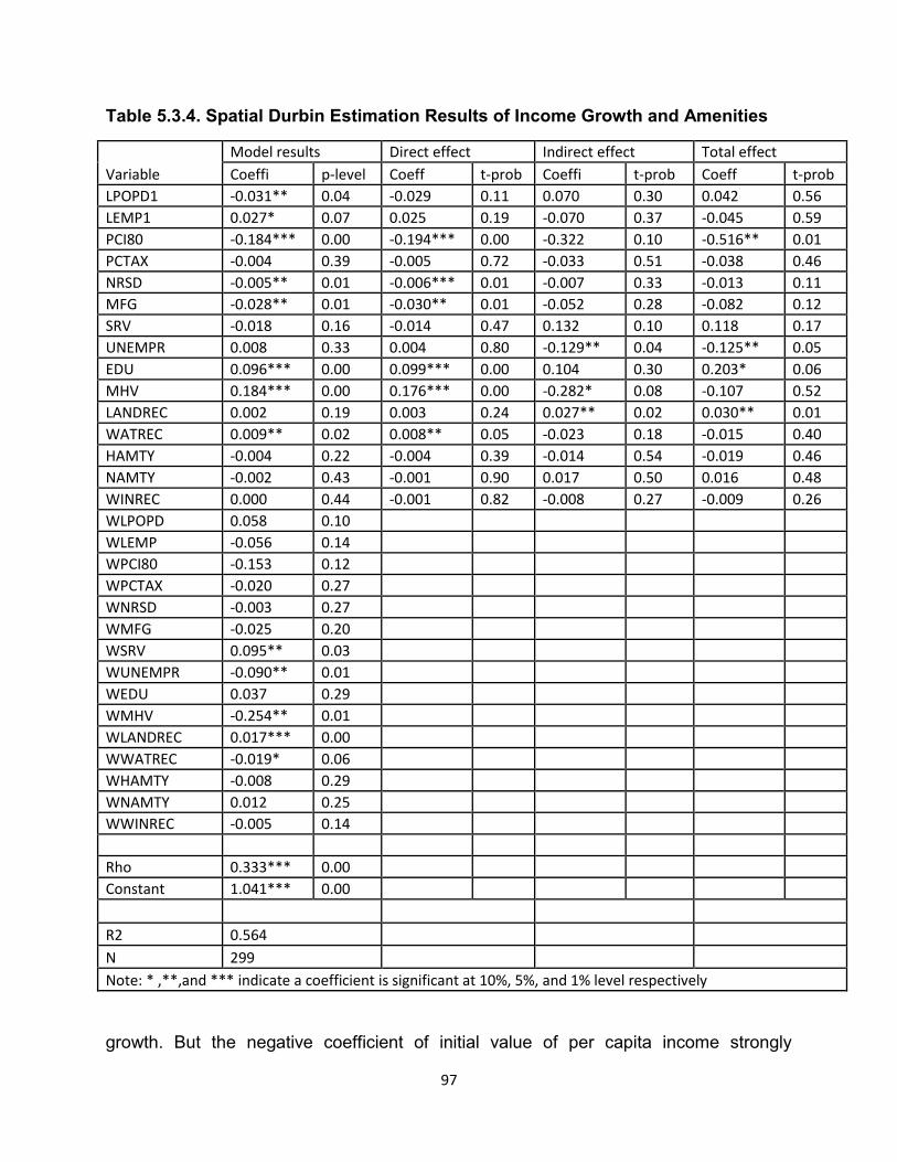
97

Table 5.3.4. Spatial Durbin Estimation Results of Income Growth and Amenities


Variable Coeffi p-level Coeff t-prob Coeffi t-prob Coeff t-prob

LPOPD1 -0.031** 0.04 -0.029 0.11 0.070 0.30 0.042 0.56

LEMP1 0.027* 0.07 0.025 0.19 -0.070 0.37 -0.045 0.59

PCI80 -0.184*** 0.00 -0.194*** 0.00 -0.322 0.10 -0.516** 0.01

PCTAX -0.004 0.39 -0.005 0.72 -0.033 0.51 -0.038 0.46

NRSD -0.005** 0.01 -0.006*** 0.01 -0.007 0.33 -0.013 0.11

MFG -0.028** 0.01 -0.030** 0.01 -0.052 0.28 -0.082 0.12

SRV -0.018 0.16 -0.014 0.47 0.132 0.10 0.118 0.17

UNEMPR 0.008 0.33 0.004 0.80 -0.129** 0.04 -0.125** 0.05

EDU 0.096*** 0.00 0.099*** 0.00 0.104 0.30 0.203* 0.06

MHV 0.184*** 0.00 0.176*** 0.00 -0.282* 0.08 -0.107 0.52

LANDREC 0.002 0.19 0.003 0.24 0.027** 0.02 0.030** 0.01

WATREC 0.009** 0.02 0.008** 0.05 -0.023 0.18 -0.015 0.40

HAMTY -0.004 0.22 -0.004 0.39 -0.014 0.54 -0.019 0.46

NAMTY -0.002 0.43 -0.001 0.90 0.017 0.50 0.016 0.48

WINREC 0.000 0.44 -0.001 0.82 -0.008 0.27 -0.009 0.26

WLPOPD 0.058 0.10

WLEMP -0.056 0.14

WPCI80 -0.153 0.12

WPCTAX -0.020 0.27

WNRSD -0.003 0.27

WMFG -0.025 0.20

WSRV 0.095** 0.03

WUNEMPR -0.090** 0.01

WEDU 0.037 0.29

WMHV -0.254** 0.01

WLANDREC 0.017*** 0.00

WWATREC -0.019* 0.06

WHAMTY -0.008 0.29

WNAMTY 0.012 0.25

WWINREC -0.005 0.14

Rho 0.333*** 0.00

Constant 1.041*** 0.00

R2 0.564

N 299


growth. But the negative coefficient of initial value of per capita income strongly

98

reinforces the result of the nonspatial model (-0.480 for nonspatial and -0.516 for the

spatial). This negative and significant relationship suggests that counties with lower

income initially experienced greater income growth than counties with higher incomes in

the earlier period.

Only two of the amenity variables are significant. Areas with higher levels of

water based recreational facilities are associated with high levels of per capita income.

The spillover effect of land based recreational facilities is positive which highlights the

importance of surrounding counties in income growth. Again as in the case of the

nonspatial model, these findings support the arguments of Wu and Mishra (2008) and

the findings of Deller and Leldo (2008) which are discussed above.

Median housing value is a major direct factor in driving per capita income in the

region. The strong positive direct effect of median value of owner occupied housing

suggests that growth in per capita income is high in areas where the median housing

values is high as in VT and NH. But the indirect effect is negative and high in magnitude

which indicates median values of surrounding counties discourages income growth.

The positive and significant coefficient of high level of college education indicates

a high educational attainment leads to high level of per capita income. In contrast to the

nonspatial model, the relationship between the proportion of a county’s population with

a bachelor’s degree or higher, a measure of human capital, and per capita income

growth, indicating that counties with high human capital endowments experience high

income growth. Even though, the direct effect of the unemployment rate is insignificant,

the indirect effect is negative and significant. This suggests that a county surrounded by

counties with high unemployment rate is likely to have low income growth.

99

5.3.4. Summary Findings of Spatial Durbin Model

The main goal of the spatial growth model is to help understand the relationships

between regional growth trends and natural and built amenities. The spatial

interdependence among regional growth indicators, natural and built amenities, and

other factors that affect regional growth are modeled in the spatial Durbin method. For

this reason, growth in population density, employment density, and per capita income

are modeled as a functions of the endogenous variables (Yi) and their spatial lags

(I+W)Yi , amenity variables (Ai) and their spatial lags (I+W)Ai, and other local factors (X)

and their spatial lags (I+W)Xi that are expected to affect regional growth. This section

provides a summary of the major findings of the estimated results.

County population growth is directly affected by employment and per capita

income growth within the county. Amenities within the county and/or surrounding

counties play a significant role in the process of population growth. Historical and

cultural amenities like museums, historical sites, zoos, and other attractions play

a positive direct and indirect role in attracting new immigrants. While the direct

effect of the natural amenity (NAMTY) is negative, the indirect effect coming from

surrounding counties is positive. This is an important finding with major policy

implications. This implies that a county that lacks natural attractions of its own

can still benefit from the natural richness of its surrounding counties. From the

local factors, median housing value, earnings from natural resource sector and

manufacturing sector are important factors in affecting population growth.

County employment density growth is significantly driven by growth in population

density and per capita income. The relationship of amenities with employment

growth generally is either negative or insignificant. There is no positive and direct

100

effect found in the relationship. The direct effects of natural amenities and land

based recreational facilities are negative but the indirect effect of historical and

cultural amenities is positive. Local factors such as earnings in the natural

resource and manufacturing sectors, direct local government expenditures, and

per capita taxes also play a role in influencing employment growth.

County per capita income growth is directly affected by water related recreational

facilities within the county and land based recreational facilities of surrounding

counties. The rest of the amenity variables do not directly or indirectly affect per

capita income growth. Both, the endogenous variables, population and

employment densities do not play a significant role in influencing income growth.

But the initial level of per capita income is negative and significant indicating that

counties with lower incomes initially experienced greater income growth than

counties with higher income in the earlier period. Earnings in manufacturing and

natural resource sectors, median housing values, and college education are the

major local and nonlocal factors affecting income growth.

101

CHAPTER 6: SUMMARY AND CONCLUSIONS

6.1. Introduction

The main objective of this research is to examine the association between

natural and built amenities and regional economic growth among counties in the

northeast region of the United States. Spatial and nonspatial models were developed

and estimated. The simultaneity nature of the dependent variables is accounted for by

using three stage least squares in the nonspatial model and two stage least squares in

the spatial Durbin model. The Northeast region of the United States is used as a study

area. It is composed of 12 states and consists 299 counties of which 148 are nonmetro.

It is highly urbanized with 50.5% of the counties considered as metro. Most of the

nonmetro areas are found in the Appalachian portion of the region. Although the region

as a whole has very few poverty persistent counties compared to the US, it has the

highest population loss counties (21.7%) due to out-migration. In this final chapter,

Summary and Conclusions, policy implications, limitations and future work related to the

study are discussed.

6.2. Summary and Conclusion

As indicated above, the primary objective of this research is to evaluate the

relationship between natural and built amenities and regional economic growth among

counties in the northeast region of the United States. The general conclusion of the

study is that, indeed, some amenities were positively associated with regional economic

growth during the 1980-2005 period. But there is no evidence of a consistent and strong

relationship. At best, the results are mixed and inconclusive. Based on the estimated

102

results, this study contributes by providing policy makers with information on the role of

natural and recreational amenities in rural economic development in the Northeast

region.

To estimate the models, a database of natural and built amenities, socio-

economic, and fiscal variables of the northeast region from 1980 to 2005 was compiled.

Nonspatial and spatial econometric models were empirically developed and estimated.

A system of equations was used to examine relationships between regional economic

growth indicators (growth in population density, employment density, and per capita

income) and natural and built amenities.

In the nonspatial estimation, ordinary least squares and three stage-least-

squares with amenity slope shifters for the northeast were applied. These slope shifters

were included to see whether amenities in rural northeast behave in different ways from

the rest of rural America. As presented in Table 5.2.1-5.2.3, clearly many of the slope

shifters were significant indicating amenities in rural northeast behaved differently from

the rest of the country. These results indicate that conclusions based on generalization

from national level analyses could be misleading. Different regions have different

natural and built amenities which could have region specific effects.

Generally, amenity indicators were hypothesized to play a positive role in

population growth. In the growth of population density equation, natural (NAMTY) and

built amenities (specifically HAMTY and WATREC) play opposing roles in shaping the

growth rate of population density of the northeast region of the US. Amenities, except

for land based recreational facilities, generally are found to have no role in determining

employment density growth. Water based recreational amenities are found to be the

103

only amenity variable that positively influences the growth in per capita income in the

last quarter of the 20th century. From all these findings, it is clear that natural amenities,

historical and cultural amenities, water and land based recreational facilities play a role

in shaping the economic growth of the northeast region. Surprisingly enough, even

though the region is endowed with winter based recreational facilities, it did not show an

influence in the process of regional economic growth.

A modified version of the spatial Durbin model (Lesage and Pace, 2009) is used

to estimate the spatial distribution of amenities and regional economic growth. To

account for the simultaneity in the dependent variables, first a reduced form is estimated

to generate the fitted values of the dependent variables. These estimated dependent

variables are then included as any other independent variable in estimating the spatial

Durbin model. Therefore, each of the three equations in the model are estimated as a

function of the fitted endogenous dependent variables (LPOPD, LEMPD, and LPCI),

spatially weighted fitted dependent variables (WLPOPD, WLEMPD, and WLPCI),

independent variables (vector X), spatially weighted independent variables (WX). This

method helped to examine not only the strength of the spatial dependence but also to

estimate the direct impacts/effects of local factors on county’s marginal economic

growth as well as a spatial spillover or indirect impact from neighboring counties. This is

the first time the spatial Durbin model has been used in assessing the relationship

between amenities and regional growth. This is one of the major contributions of this

study to the amenity and regional growth literature.

The results of the spatial impact of amenities on regional economic growth are

mixed. Amenities within a county and/ or surrounding counties play a significant role in

104

the process of population growth. Historical and cultural amenities like museums,

historical sites, zoos, and other attractions play a positive direct and indirect role in

attracting new immigrants. While the direct effect of natural amenity (NAMTY) was

negative, the indirect effect coming from surrounding counties was positive. This is an

important finding with major policy implications. This implies that a county that lacks

natural attractions of its own can still benefit from the natural richness of its surrounding

counties.

The relationship of amenities with employment growth was either negative or

insignificant. There was no positive direct effect found. The direct effect of natural

amenities and land based recreational facilities were negative but the indirect effect of

historical and cultural amenities was positive. County per capita income growth is

directly affected by water related recreational facilities within the county and land based

recreational facilities of surrounding counties (both positive). Given these mixed results

and the fact that the total effect of historical and cultural amenities (in two of the three

equations) was positive and the total effect of land based recreational facilities was

mixed (negative in two and positive in one), we cannot ignore the role of amenities.

One possible reason for these mixed and weak relationships is the choice of the sample

data.

As discussed in chapter five, the spatial model was estimated using data for all

metro and nonmetro counties. Therefore, the estimated coefficients are the average

direct and indirect effects of the metro and nonmetro areas. Given that the region is

highly urbanized and economically diversified, the effects of amenities is dwarfed by

other socio-economic factors that are in play in the region. Consequently, many of the

105

amenity factors that were expected to play an important role on the regional economic

growth of nonmetro counties became insignificant or minor players. However, the

results of the spatial estimation of the nonmetro counties (Table 5.3.5-5.3.6 in the

appendix), even with all its limitations discussed in chapter five, show that with the

exception of winter based recreational facilities, the rest of the amenity indices play a

significant but inconsistent role in the economic growth of the region.

Using a national data set of all nonmetro counties, the role of proximity to the

demand market and accessibility to supply of amenities was tested. The results were

contrary to the expectations. No relationship was detected between the proximity to the

amenity demand market and all three measures of regional growth. The test was

conducted using an interaction term of natural amenity measure and adjacency to metro

area as proxy to proximity to the amenity demand market. One of the reasons for this

finding could be the choice of proxy. There is no clear cut relationship between regional

growth indicators and the proxy for the supply of natural amenities (NAMTYHWD). In

line with expectations, it was positive and significant in the population growth equation

indicating accessibility to the supply of amenities matters. But it was negative and

significant for the employment and income growth equations which show accessibility to

the supply of amenities depresses regional growth. There are no logical explanations for

these two contradicting results. In all cases, its magnitude was very small which

diminishes its significance as a major determining factor.

One of the hypotheses tested in this study was the role of economic activities of

surrounding counties. It was hypothesized that growth is conditional and affected by

economic activities in surrounding counties. The results of the spatial Durbin model give

106

evidence for this test. In addition to the indirect effects (positive and negative) of

amenities discussed above, high dependence on natural resource and manufacturing

sectors, and unemployment rate in the surrounding counties are found to depress

regional economic growth by exerting negative influences on population and

employment growth.

6.3. Policy Recommendations Based on empirical findings of this study a couple of recommendations can be

suggested for effective application of amenity-led development in the northeastern

United States.

The findings of the study show that historical and cultural amenity and water

based recreational facilities were positively associated with regional economic

growth during the 1980-2005 period. Given this fact, preservation of historical

and cultural sites and development of water based recreational sites should be

encouraged. The presence of these local attributes could encourage not only

people to live and stay in these areas but also to attract new migrants. But the

preservation of amenities has an opportunity cost and the decision should be on

a case by case based. Therefore, local policy makers should identify, preserve,

develop, and promote only attributes that has the potential to serve as a

development strategy.

Regional cooperation in preservation, development and management of natural

resources and recreational facilities should be one of the main strategies in

developing amenity- led development. The results show a positive spatial

spillover effect of natural and historical and cultural amenities as well as land

107

based recreational facilities. Then the question policy makers have to address is

how are these resources managed and funded? Generally amenities are public

goods. If the cost of maintenance and development is left to the county within

which they reside, they will tend to be underfunded and underdeveloped.

Regional internalization of this positive externality is required to take full

advantage of the natural asset in the regional economic growth process.

While there are some similarities across the United States, the country is

sufficiently heterogeneous that the impact of amenities or other policy variables

may be significantly different depending on where one is within the country.

Specifically, the coefficients of the amenity slope shifters in the results suggest

that the non-metropolitan northeast region follows different pattern. These

findings should be recognized by regional policy makers in developing regional

policies. Policies developed based on generalization of national level analyses

could be misleading. Thus, understanding the spatial distribution of local

amenities within the specific region is an important factor for promoting amenity-

led development.

6.4. Limitations and Future Research

6.4.1. Limitations

The main contribution of the study is its ability to estimate the direct and indirect

effects of amenities on regional economic growth. But this is also one of its limitations.

As discussed in Chapter 5, the spatial model was estimated using data for all metro and

nonmetro counties. This was done to capture the spillover effects from the metro

counties surrounding the nonmetro counties. Therefore, the estimated coefficients are

the average direct and indirect effect of the metro and nonmetro counties. Given that

108

the region is highly urbanized and economically diversified, the effects of amenities is

dwarfed by other socio-economic factors that are in play in the region. Consequently,

many of the amenity factors that were expected to play an important role on the regional

economic growth of nonmetro counties became insignificant or minor players.

The amenity data used in the study was compiled from the USDA Forest Service,

National Outdoor Recreation Supply Information System (NORSIS). Even though, it is

the most comprehensive database available for amenity related studies, it is by no

means exhaustive. Furthermore, the way the amenity indices were constructed also has

its limitations. The study followed the literature in selecting the different attributes that

formed the indices. There is no standard or theoretical base for including or excluding

different amenity attributes. Different combinations of attributes could be used and could

produce different results.

The weight matrix used in the spatial estimation was based on the nearest eight

neighbors. There is no rule that guides the construction of a weight matrix. A weight

matrix constructed based on contiguity, distance, and other choices of neighbors could

give different results.

6.4.2. Future Research

There are several ways this study could be extended. Additional research in this

area could focus on and significantly contribute to the knowledge of amenity-led

development by expanding into the following areas:

1. Finding a mechanism to apply the spatial Durbin model to nonmetro counties but

using all relevant counties to construct the weight matrix could help to solve the current

estimation challenge. This could help to estimate the impact of amenities on nonmetro

counties.

109

2. The spatial results are based on one form of weight matrix. Developing a different

weight matrix could lead to different results. Generating different results for each of the

weight matrix using the spatial Durbin model and comparing these results could show

the overall impact of the spatial distribution of amenities.

3. Extending this study to include all nonmetro counties in the US can be a next logical

step. This can enrich the study by providing a bigger sample size and variability in the

dataset.

4. Estimating the impact of specific amenities (not indices) in a specific county or group

of counties by conducting a case study could lead to more practical policy implications.

110

REFERENCES Anselin, Luc, (1988). Spatial Econometrics: Methods and Models. Kluwer Academic

Press, Dordrecht. Anselin, Luc, and Anil K. Bera. (1998). Spatial Dependence in Linear Regression

Models with an Introduction to Spatial Econometrics. In Aman Ullah and David Giles (Eds.). Handbook of Applied Economic Statistics (pp. 237-289). New York: Marcel Dekke

Beale, C.L, and K.M. Johnson (1998). “The Identification of Recreational Counties in

Nonmetropolitan Area of the USA.” Pop. Res. Policy Rev. 17:37-53

Blanchflower, D.G. and Oswald, A.J. (1996). The Wage Curve. Cambridge, MA:MIT

Press.

Boarnet, M.G. 1995. “Transportation Infrastructure, Economic Productivity, and

Geographic Scale: Aggregate Growth versus Spatial Distribution.” Available

online at http://www.uctc.net/papers/255.pdf

Carlino, G.A. and Mills, E.S. (1987). “The Determinants of County Growth.” Journal of

Regional Science, 27, 39–54

Carruthers JI, Hollar MK, Mulligan, GF (2006). “Growth and Convergence in the Space

Economy: Evidence from the United States.” Presented at the 46th Congress of

the European Regional Science Association, August 30-Spetember 3, 2006 in

Volos, Greece

Cromartie, J.B. (2001). “Migrants in the Rural South Choose Urban and Natural

Amenities.” Rural America 15, 7–18.

Duncombe, W., M. Robbins and D. Wolf. (2000). “Chasing the elderly: Can State and

Local Governments Attract Recent Retirees?” Paper No. 22. Syracuse, NY:

Center for Policy Research, Maxwell School of Citizenship and Public Affairs,

Syracuse University.

Deller and Victor Lledo (2007). “Amenities and Rural Appalachia Economic Growth.”

Agricultural and Resource Economics Review, 36:107-132.

Deller and Victor Lledo, and Marcouiller W.D. (2008). “Modelling Regional Economic

Growth with a Focus on Amenities.” Review of Urban and Regional Development

Studies, 20,1-21

Deller, C.D., Tsai, T.-H.S.M. and English, B.K.D. and V. Liedo (2005). “Regional

Economic Growth with a Focus on Amenities.” In “Amenities and Rural

111

Development: Theory, Methods and Public Policy.” G.P. Green, S.C. Deller, and

D.W. Marcouiller, eds., Northampton, MA: Edward Elgar.

Deller, C.D., Tsai, T.-H.S.M. and English, B.K.D. (2001). “The Role of Amenities and

Quality of Life in Rural Economic Growth.” American Journal of Agricultural

Economics 83, 352–365.

Deller, S.C. and Tsai, T.S. (1999). “An Examination of the Wage Curve. A Research

Note.” Journal of Regional Analysis and Policy 28, 3–12.

Dissart, Jean-Christophe. (2007). “Landscapes and regional development: What are the links?” Cahiers d’économie et sociologie rurales, n° 84-85.

Doreian, Patrick. (1980). “Linear Models with Spatially Distribute Data: Spatial

Disturbances or Spatial Effects.” Sociological Methods & Research 9(1): 29-60. ……… (1981). “Estimating Linear Models with Spatially Distributed Data”. In Samuel

Leinhardt (Ed.). “Sociological Methodology” (pp. 359-388). San Francisco, CA: The Jossey-Bsess Inc.

Duffy-Deno, K.T. (1997a). “The Effect of State Parks on the County Economies of the

West.” Journal of Leisure Research, 29, 201–2224.

_________ (1998). “The Effect of Federal Wilderness on County Growth in the

Intermountain Western US.” Journal of Regional Science 38, 109–136.

Economic Research Service (ERS)(1999). Natural Amenities Scale Available from:

http://www.ers.usda.gov/emphases/rural/data/amenities

English, D.B.K., Marcouiller, D.W. and Cordell, H.K. (2000). “Linking Local Amenities

with Rural Tourism Incidence: Estimates and Effects.” Society and Natural

Resource 13, 185–202.

Fabian Waltert and Felix Schläpfer. (2007). “The Role of Landscape Amenities in Regional Development: A Survey of Migration, Regional Economic and Hedonic Pricing Studies.” Socioeconomic Institute, University of Zurich, Working Paper No. 0710

Galston, William A., and Karen J. Baehler. (1995). Rural Development in the United

States: Connecting Theory, Practice, and Possibilities. Washington, DC: Island

Press.

Gebremariam, G.H., T.G. Gebremedhin, and P.V. Schaeffer. (2006). “An Empirical

Analysis of County-Level Determinants of Small Business Growth in Appalachia:

112

A Spatial Simultaneous-Equations Approach.” Paper presented at the Southern

Agricultural Economics Association Annual Meeting, Orlando, FL (February 5–8).

Gibson, Lay James. (1993). “The Potential for Tourism Development in Nonmetropolitan

Areas,” in David L. Barkley, ed., “Economic Adaptation: Alternatives for

Nonmetropolitan Areas”, pp. 145-64. Boulder, CO: West-view Press.

Goe, W.R., and G.P. Green. 2005. “Analyzing the Relation-ship Between Amenities and

Change in the Well-Being of Nonmetropolitan Localities.” “In Amenities and Rural

Development: Theory, Methods and Public Policy.” G.P. Green, S.C. Deller, and

D.W. Marcouiller, eds., Northampton, MA: Edward Elgar.

Golding, Shaun A. and Auken, Paul M. Van. (2006). “Amenities and Inequality in Rural

America: A preliminary Spatial Analysis.” Paper presented at the Population

Association of America Annual Meeting

Gottlieb, P.D. (1994). “Amenities as an Economic Development Tool: Is There Enough

Evidence?” Economic Development Quarterly 8, 270–285.

Gottlieb, P.D. (1995). “Residential Amenities, Firm Location and Economic Development”, Urban Studies, Vol. 32, No. 9, 1413-1436

Graves,P.E. and Muser, P.R. (1993). “The Role of Equilibruim and Disequilibruim in

Modeling Regional Growth and Decline.A critical Reassessment.” Journal of

Regional Science, 33

Green, G.P. (2001). “Amenities and Community Economic Development: Strategies for

Sustainability.” Journal of Regional Analysis and Policy 31, 61–76.

Gunderson, Ronald J. and Ng Pint T. (2006). “Summarizing The Effect of Wide Array

of Amenity into Simple Components.” Social Indicators Research 79: 313–335

Hailu, Y.G., and C. Brown. (2006). “A Spatial Simultaneous Growth Equilibrium

Modeling of Agricultural Land Development in the Northeast United States.”

Paper presented at the American Agricultural Economics Association Annual

Meeting, Long Beach, CA (July 23–26).

______. 2007. “Regional Growth Impacts on Agricultural Land Development: A Spatial

for Three States.” Agricultural and Resource Economics Review 36(1)

Henderson, J. and K. McDaniel. (1998). “Do scenic amenities foster economic growth in

rural areas?” Federal Reserve Bank of Kansas City, Regional Economic Digest,

1st quarter:11-17.

113

Henderson, J. and K. McDaniel. (2005). “Natural Amenities and Rural Employment

Growth: A Sector Analysis.” The Review of Regional Science 35(1)

Hoehn, J.P., Berger, M.C., Blomquist, G.C., (1987). “A Hedonic Model of Interregional Wages, Rents, and Amenity Values.” Journal of Regional Science 27 (4), 605-620.

Judson, D.H., S. Reynolds-Scanlon, and C.L. Popoff. (1999). “Migrants to Oregon in the

1990’s: Working age, near-retirees, and retirees make different destination

choices.” Rural Development Perspectives 14:24–31.

Keith, John, and Christopher Fawson. (1995). “Economic Development in Rural Utah: Is

Wilderness Recreation the Answer?” Annals of Regional Science. 29,3: 303-313

Kim, K., Marcouiller, D.W., Deller, S.C., (2005). “Natural Amenities and Rural Development: Understanding Spatial and Distributional Attributes.” Growth and Change 36 (2), 273-297.

Kirby, Dustin K. and LeSage, James P. (2009). “Changes in commuting to work times

over the 1990 to 2000 period.” Regional Science and Urban Economics LeSage, James P (1997). “Regression Analysis of Spatial Data.” Journal of Regional

Analysis and Policy, 27(2),83-94 LeSage, James P. and R. Kelly Pace. (2009). Introduction to Spatial Econometrics.

CRS Press

Lewis, D.J., Hunt, G.L., Plantinga, A.J., (2002). “Public Conservation Land and Employment Growth in the Northern Forest Region.” Land Economics 78 (2), 245-259.

Lewis, D.J., Hunt, G.L., Plantinga, A.J., (2003). “Does Public Lands Policy Affect Local

Wage Growth?” Growth and Change 34 (1), 64-86. Marcouiller, David W., and Gary Paul Green. (2000). “Outdoor Recreation and Rural

Development.” In Gary E. Machlis and Donald R. Field, eds., “National Parks and

Rural Development: Practice and Policy in the United States”, Washington, DC:

Island Press

Marcouiller, D.W., K.K. Kim, and S.C. Deller. (2004). “Natural Amenities, Tourism and

Income Distribution.” Annals of Tourism Research 31(4): 1031–1050.

MacDonald, John F., (1992). “Assessing the Development Status of Metropolitan Areas”, in Edwin S.Mills and John F. MacDonald (ed.), “Sources of Metropolitan Growth”, New Brunswick, NJ: Center for Urban Policy Research.

114

McGranahan, D.A. (1999). Natural Amenities Drive Rural Population Change. Food and

Rural Economics Division, Economic Research Service, US Department of

Agriculture. [AER-781], 1–24.

MaGranhan, D.A. and Beale, C.L.(2003). The Roots of Rural Population Loss. Amber

Waves.

Monchuk, Daniel. (2003). “The Role of Amenities on Employment Growth in the U.S.

Heartland: A Spatial Analysis Examining the Role of Recreational Amenities in

Surrounding Counties.” Working Paper: Iowa State University Ames, Iowa 2003

Northeastern Regional Center for Rural Development (NRCRD). “Regional Listening Sessions on Rural Entrepreneurship: Lessons from Northeast.” Rural Development Paper No. 37, July 2007.

Nzaku, Kilungu and James Bukenya (2005). “Examining the relationship between

Quality of Life Amenities and Economic Development in the Southeast USA.”

Review of Urban and Regional Development Studies Vol. 17, No. 2, July 2005.

Nord, M. and Cromartie, J.B. (1997). “Migration: The Increasing Importance of Rural

Natural Amenities.” Choices 3, 22–23.

Ohman, Debra. (1999). “Restructuring and Well-being in the nonmetropolitan Pacfic

Northwest.” Growth and Change, 30, 161-183

Organization for Economic Cooperation and Development (OECD). (1994). The

Contributions of Amenities to Rural Development. Paris: OECD

Power, Thomas M. (1988). The Economic Pursuit of Quality. Armonk, NY: M.E.

Sharpe, Inc.

………. ….(1996). Lost Landscapes and Failed Economies. Washington, D.C.: Island

Press.

…………..(2005). “The supply and demand for natural amenities: An overview of theory and concepts.” In “Amenities and Rural Development: Theory, Methods

and Public Policy.” G.P. Green, S.C. Deller, and D.W. Marcouiller, eds.,

Northampton, MA: Edward Elgar.

Rey, S.J. and M.G.Boarnet. (1998). “A Taxonomy of Spatial Econometrics Models for

Simultaneous Equations Systems.” Paper presented at the 45th Annual North

America Meetings of the Regional Science Association International, Sanata Fe,

New Mexico

115

Roback, J. (1982). “Wages, Rents, and the Quality of Life.” Journal of Political Economy

90, 1257–1277.

………… (1988). “Wages, Rents, and Amenities: Differences among Workers and

Regions.” Economic Inquiry 26(1): 23–41.

Rudzitis, G. (1999). “Amenities Increasingly Draw People to the Rural West.” Rural

Development Perspective. 14: 9-13.

Shaffer R., Deller S. and Marcouiller D.( 2006). “Rethinking Community Economic

Development.” Economic Development Quarterly; 20: 59-74

Shields M., Goetz S.J., and Wang Quiyan (2005). “Out-migration from the Northeast

US: The Relative roles of Economic and Amenity Differentials.” In “Amenities and

Rural Development: Theory, Methods and Public Policy.” G.P. Green, S.C.

Deller, and D.W. Marcouiller, eds., Northampton, MA: Edward Elgar.

Steinnes, D., and W. Fisher. (1974). “An Econometric Model of Intraurban Location.”

Journal of Regional Science 14(1): 65–80.

Treyz, G.I., D.S. Rickman, G.L. Hunt, and M.J. Greenwood. (1993). “The Dynamics of

U.S. Internal Migration.” Review of Economics and Statistics 75(2): 209–214.

USDA, Economic Research Service (ERS). “Urban Influence Code (1993).” [Online] available from http://www.ers.usda.gov/Data/UrbanInfluenceCodes/2003; accessed 17 June 2008.

US Census Bureau. 1980. Selected Historical Decennial Census, Urban and Rural

Definitions and Data. Available from: http://www.census.gov/population.

accessed 15 June 2008

US Department of Commerce, Bureau of Economic Analysis. 1980-2005. Interactive

Regional Data [Internet document]. Available from:

http://www.bea.doc.gov/bea/regional/reis/default.cfm accessed 14 June 2008

USDA Forest Service, National Outdoor Recreation Supply Information System

(NORSIS 1997). available upon request from USDA Forest Service Southern

Station

Vias, A.C., and G.F. Mulligan. (1999). “Integrating Economic Base Theory with Regional Adjustment Models: The Nonmetropolitan Rocky Mountain West Region.” Growth and Change 30: 507-525.

116

White, Kristopher D. and Hannik, Dean M. (2003), “Moderate Environmental Amenities

and Economic Change: The Nonmetropolitan Northern Forest of the Northeast

U.S.”, 1970-2000, Growth and Change 35(1): 42-60

Wooldridge J.M. (2002). “Econometric Analysis of Cross Section and Panel Data.” The

MIT Press

Wu, JunJie., and Mishra,Sanjiv (2007). “Natural Amenities, Human Capital, and

Economic Growth: An Empirical Analysis.” In “Frontiers in Resource and Rural

Economics.” JunJie Wu, Paul W. Barkley, and Bruce A. Weber (eds). RFF Press

Yang, Tse-Chuan, and Anastasia R. Snyder, 2007. “Population Change in the Northeast

2000-2005",The Northeast Regional Center for Rural Development RDP No. 39,

available at http://nercrd.psu.edu/Publications/rdppapers/rdp39.pdf

117

APPENDICES Figure 4.1. Climate Index

Figure 4.2. Natural Resource Amenities

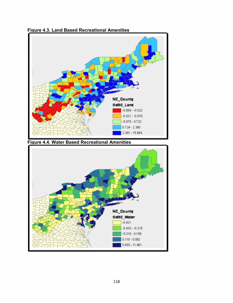
118

Figure 4.3. Land Based Recreational Amenities

Figure 4.4. Water Based Recreational Amenities

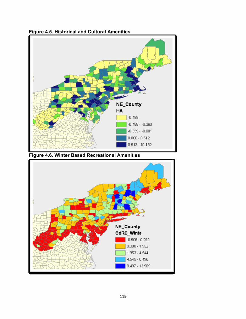
119

Figure 4.5. Historical and Cultural Amenities

Figure 4.6. Winter Based Recreational Amenities

120

Table 5.3.5. Spatial Durbin Estimation Results of Population Growth and Amenities



LEMPD -0.031 0.45 -0.051 0.81 -1.699** 0.029 -1.750** 0.03

LPCI 1.721** 0.03 1.805* 0.07 6.818** 0.034 8.623*** 0.01

POPD80 -0.172*** 0.00 -0.170*** 0.00 0.171 0.421 0.001 1.00

DLGEXP 0.060 0.40 0.055 0.83 -0.406 0.643 -0.352 0.72

PCTAX -0.199 0.12 -0.200 0.26 -0.071 0.933 -0.271 0.77

NRSD -0.008 0.32 -0.008 0.65 0.012 0.845 0.004 0.95

MFG -0.171* 0.05 -0.171 0.10 0.043 0.910 -0.128 0.76

UNEMPR -0.083 0.29 -0.085 0.57 -0.114 0.819 -0.199 0.69

MHV 1.515*** 0.00 1.535*** 0.00 1.329 0.436 2.865 0.10

UIFC -0.008 0.40 -0.011 0.73 -0.265* 0.084 -0.276* 0.09

LANDREC 0.078 0.11 0.078 0.22 0.009 0.970 0.087 0.72

WATREC 0.154** 0.03 0.165** 0.05 0.910** 0.014 1.075** 0.01

HAMTY 0.274*** 0.00 0.279*** 0.00 0.275 0.397 0.553 0.12

NAMTY -0.192*** 0.00 -0.189*** 0.00 0.349* 0.068 0.160 0.35

WINREC 0.015 0.24 0.016 0.47 0.069 0.415 0.084 0.35

WLEMPD -1.485*** 0.00

WLPCI 5.763*** 0.01

WPOPD80 0.174 0.17

WDLGEXP -0.360 0.32

WPCTAX -0.042 0.46

WNRSD 0.011 0.42

WMFG 0.062 0.43

WUNEMPR -0.087 0.42

WMHV 0.964 0.24

WUIFC -0.231** 0.03


WWATREC 0.778*** 0.00

WHAMTY 0.205 0.22

WNAMTY 0.332** 0.02

WWINREC 0.059 0.20

rho 0.101 0.27

constant -5.282** 0.04

R2 0.777

N 148


121

Table 5.3.6. Spatial Durbin Estimation Results of Employment Growth and Amenities



POPD 0.616*** 0.00 0.614*** 0.00 -0.469 0.45 0.146 0.82

LPCI 0.910 0.15 0.918 0.29 0.625 0.79 1.543 0.52

EMPD80 0.0003 0.36 0.0003 0.68 0.004 0.21 0.004 0.21

DLGEXP -0.196 0.18 -0.194 0.40 0.384 0.65 0.190 0.84

PCPTAX 0.215* 0.08 0.209 0.18 -0.784 0.30 -0.575 0.49

NRSD -0.030** 0.03 -0.030** 0.05 -0.074 0.23 -0.104 0.12

MFG -0.142* 0.08 -0.143 0.15 0.010 0.98 -0.133 0.77

SRV 0.348*** 0.01 0.344** 0.03 -0.490 0.34 -0.146 0.79

EDU -0.277 0.12 -0.271 0.25 0.766 0.33 0.495 0.54

UIFC 0.095*** 0.00 0.094*** 0.01 -0.126 0.36 -0.031 0.83

LANDREC -0.043 0.23 -0.044 0.45 -0.084 0.66 -0.128 0.51

WATREC 0.020 0.39 0.025 0.74 0.477* 0.09 0.501* 0.09

HAMTY 0.122** 0.03 0.125* 0.07 0.315 0.26 0.440 0.15

NAMTY -0.205*** 0.00 -0.203*** 0.00 0.296 0.10 0.092 0.57

WINREC 0.012 0.27 0.013 0.50 0.039 0.54 0.052 0.44

WPOPD1 -0.486 0.19

WLPCI1 0.479 0.40

WEMPD80 0.004* 0.09

WDLGEXP 0.367 0.31

WPCPTAX -0.729 0.14

WNRSD -0.063 0.12

WMFG 0.026 0.48

WSRV -0.475 0.15

WEDU 0.717 0.15

WUIFC -0.123 0.16


WWATREC 0.427** 0.03

WHAMTY 0.271 0.12

WNAMTY 0.288** 0.04

WWINREC 0.034 0.26

Rho 0.072 0.33

constant -0.134 0.49

R2 0.664

N 148


122

Table 5.3.7. Spatial Durbin Estimation Results of Income Growth and Amenities



LPOPD1 0.020 0.29 0.024 0.50 -0.157 0.16 -0.132 0.25

LEMP1 -0.008 0.40 -0.008 0.82 -0.029 0.73 -0.036 0.68

PCI80 -0.333*** 0.00 -0.329*** 0.00 -0.189 0.41 -0.518** 0.02

PCTAX 0.023 0.14 0.024 0.27 -0.027 0.65 -0.003 0.96

NRSD -0.004** 0.03 -0.004* 0.08 -0.004 0.60 -0.008 0.30

MFG -0.019 0.13 -0.018 0.29 -0.044 0.36 -0.062 0.24

SRV 0.044** 0.04 0.042* 0.09 0.054 0.46 0.096 0.21

UNEMPR -0.016 0.24 -0.012 0.62 -0.155** 0.02 -0.167*** 0.01

EDU 0.066* 0.07 0.067 0.13 -0.016 0.86 0.051 0.58

MHV 0.110 0.11 0.099 0.29 0.432 0.12 0.53** 0.05

LANDREC -0.017** 0.02 -0.016* 0.08 -0.051* 0.07 -0.067** 0.02

WATREC 0.029*** 0.01 0.028** 0.03 0.036 0.34 0.064 0.10

HAMTY -0.008 0.22 -0.009 0.39 0.025 0.43 0.016 0.64

NAMTY 0.003 0.39 0.001 0.92 0.069** 0.02 0.07** 0.02

WINREC -0.001 0.38 -0.001 0.77 0.000 0.96 -0.001 0.91

WLPOPD -0.183* 0.08

WLEMP -0.036 0.36

WPCI80 -0.304 0.11

WPCTAX -0.027 0.35

WNRSD -0.005 0.26

WMFG -0.057 0.15

WSRV 0.075 0.19

WUNEMPR -0.189*** 0.00

WEDU -0.004 0.49

WMHV 0.543** 0.04

WLANDREC -0.065** 0.02

WWATREC 0.050 0.12

WHAMTY 0.027 0.23

WNAMTY 0.083*** 0.01

WWINREC 0.000 0.50

Rho -0.265 0.10

Constant 1.614*** 0.00

R2 0.67

N 148


Documents

An analysis of amenity-led rural economic *development in