ORIGINAL PAPER

An alternative method to characterize the surface urbanheat island

Philippe Martin & Yves Baudouin & Philippe Gachon

Received: 26 June 2013 /Revised: 5 September 2014 /Accepted: 5 September 2014 /Published online: 19 September 2014# The Author(s) 2014. This article is published with open access at Springerlink.com

Abstract An urban heat island (UHI) is a relative measuredefined as a metropolitan area that is warmer than the sur-rounding suburban or rural areas. The UHI nomenclatureincludes a surface urban heat island (SUHI) definition thatdescribes the land surface temperature (LST) differences be-tween urban and suburban areas. The complexity involved inselecting an urban core and external thermal reference forestimating the magnitude of a UHI led us to develop a newdefinition of SUHIs that excludes any rural comparison. Thethermal reference of these newly defined surface intra-urbanheat islands (SIUHIs) is based on various temperature thresh-olds above the spatial average of LSTs within the city’sadministrative limits. A time series of images from LandsatThematic Mapper (TM) and Enhanced Thematic Mapper Plus(ETM+) from 1984 to 2011 was used to estimate the LSToverthe warm season in Montreal, Québec, Canada. DifferentSIUHI categories were analyzed in consideration of the globalsolar radiation (GSR) conditions that prevailed before eachacquisition date of the Landsat images. The results show thatthe cumulative GSR observed 24 to 48 h prior to the satelliteoverpass is significantly linked with the occurrence of thehighest SIUHI categories (thresholds of +3 to +7 °C abovethe mean spatial LST within Montreal city). The highestcorrelation (≈0.8) is obtained between a pixel-based tempera-ture that is 6 °C hotter than the city’s mean LST (SIUHI+6)

after only 24 h of cumulative GSR. SIUHI+6 can then be usedas a thermal threshold that characterizes hotspots within thecity. This identification approach can be viewed as a usefulcriterion or as an initial step toward the development of heathealth watch and warning system (HHWWS), especially dur-ing the occurrence of severe heat spells across urban areas.

Keywords Urban . Rural . Surface urban heat island .

Intra-urban . Landsat imagery

AbbreviationsBLUHI Boundary layer urban heat islandCLUHI Canopy-layer urban heat islandDAI Data Access IntegrationDN Digital numberETM+ Enhanced Thematic Mapper PlusGIS Geographical information systemGSR Global solar radiationHHWWS Heat health watch and warning systemk1 Calibration constants (TM=607.76 or

ETM+=666.9)k2 Calibration constants (TM=1260.56 or

ETM+=1282.71)L Spectral radianceLST Land surface temperatureMJ Megajoule (equal to one million (106) joules)MMC Montreal Metropolitan CommunityMSC Meteorological Service of CanadaNDVI Normalized Difference Vegetation IndexNIR Near infraredP-E-T Pierre Elliott TrudeauRBL Rural boundary layerSD Standard deviationSEBAL Surface Energy Balance Algorithms for LandSIUHI Surface intra-urban heat islandSSUHI Subsurface urban heat islandSUHI Surface urban heat islandTCZ Thermal climate zoneTM Thematic Mapper

P. Martin (*)Meteorological Service of Canada, Environment Canada, Montréal,Québec, Canadae-mail: philippe.martin@ec.gc.ca

Y. BaudouinDepartment of Geography, University of Québec at Montreal(UQAM), Montréal, Canada

P. GachonCanadian Centre for Climate Modelling and Analysis (CCCMA),Climate Research Division, Environment Canada, Montréal, Canada

P. GachonESCER (Étude et Simulation du Climat à l’Échelle Régionale)Centre, University of Québec at Montréal, Montréal, Canada

Int J Biometeorol (2015) 59:849–861DOI 10.1007/s00484-014-0902-9

TOA Top of atmosphere (albedo)UBL Urban boundary layerUCL Urban canopy layerUCZ Urban climate zoneUHI Urban heat islandUSGS US Geological Survey

Introduction

Urban city centers tend to have higher solar radiation absorp-tion and greater thermal capacity and conductivity than thesurrounding area (Weng 2001). These modified thermal condi-tions can cause the local air and surface temperatures to in-crease by several degrees Celsius over the simultaneous tem-peratures of the surrounding rural areas (Oke 1982). Theseurban heat islands (UHIs) result partly from the physical prop-erties of the urban landscape and partly from the release of heatinto the environment by the use of energy for human activities.With an increasing area of impervious and man-made non-vegetated surfaces within major metropolitan cities (i.e.,through the use of paving or building materials), more of theincoming energy is converted to surface-sensible heat fluxes,thus reducing a given city’s ability to shed its excessive heat by

latent heat exchange (Oke 1987). The occurrence and intensityor severity of heat spells has been linked to the UHI effect(Clarke 1972; Rooney et al. 1998). During hot-weather events,UHIs exacerbate thermal stress on the most vulnerable and at-risk people, particularly those with social or physical vulnera-bility (Kovats and Hajat 2008; Smargiassi et al. 2009).

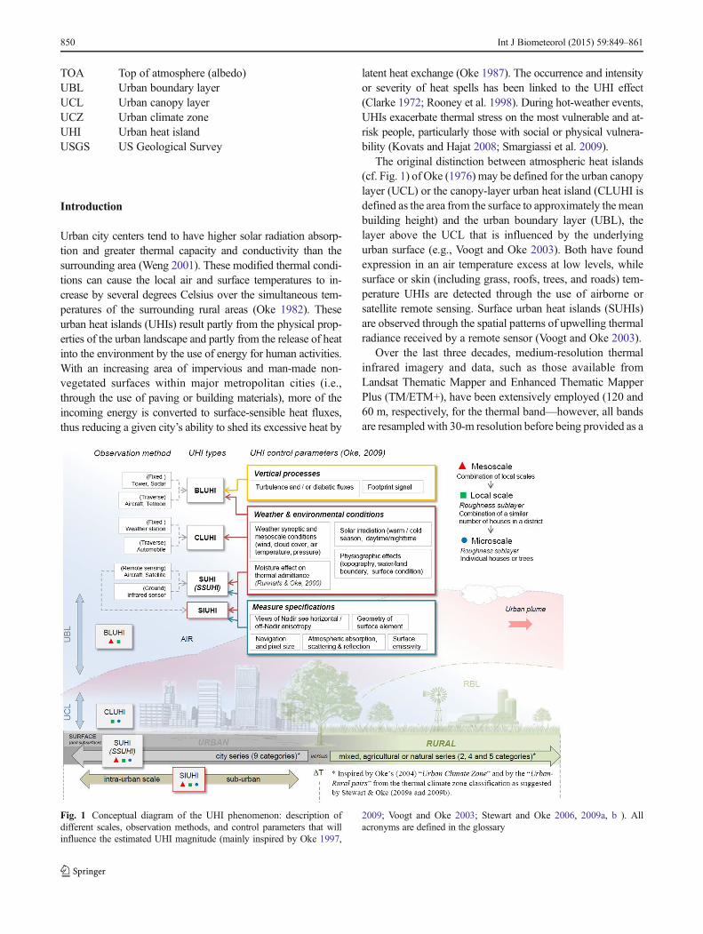
The original distinction between atmospheric heat islands(cf. Fig. 1) of Oke (1976) may be defined for the urban canopylayer (UCL) or the canopy-layer urban heat island (CLUHI isdefined as the area from the surface to approximately the meanbuilding height) and the urban boundary layer (UBL), thelayer above the UCL that is influenced by the underlyingurban surface (e.g., Voogt and Oke 2003). Both have foundexpression in an air temperature excess at low levels, whilesurface or skin (including grass, roofs, trees, and roads) tem-perature UHIs are detected through the use of airborne orsatellite remote sensing. Surface urban heat islands (SUHIs)are observed through the spatial patterns of upwelling thermalradiance received by a remote sensor (Voogt and Oke 2003).

Over the last three decades, medium-resolution thermalinfrared imagery and data, such as those available fromLandsat Thematic Mapper and Enhanced Thematic MapperPlus (TM/ETM+), have been extensively employed (120 and60 m, respectively, for the thermal band—however, all bandsare resampled with 30-m resolution before being provided as a

Fig. 1 Conceptual diagram of the UHI phenomenon: description ofdifferent scales, observation methods, and control parameters that willinfluence the estimated UHI magnitude (mainly inspired by Oke 1997,

2009; Voogt and Oke 2003; Stewart and Oke 2006, 2009a, b ). Allacronyms are defined in the glossary

850 Int J Biometeorol (2015) 59:849–861

final product by the US Geological Survey (USGS)). Thesesatellite data are appropriate for studying intra-urban tempera-ture variations and relating them to surface cover characteristics(Hafner and Kidder 1999; Kim 1992; Parlow 1999; Rigo et al.2003; Streutker 2002). Carnahan and Larson (1990) usedLandsat TM data to analyze thermal conditions in theIndianapolis metropolitan area (Indiana) and found an urban–rural radiant temperature difference of 6.4 °C in the daytime(heat sink). Using Landsat’s two sensors, Xian and Crane(2006) evaluated urban thermal characteristics in the TampaBay watershed (Florida, USA) and Las Vegas Valley (Nevada,USA) and found that Tampa Bay has a daytime heating effect(heat source), whereas Las Vegas exhibits a daytime coolingeffect (heat sink). This is due to the expected moisture status ofrural areas; where rural areas (Las Vegas) are very dry, morerapid morning heating could lead to the apparent presence of asurface cool island, while a wet rural area (Tampa Bay) wouldbe slower to warm than urban areas. Hence, the surroundings ofa city, which are used as thermal references for evaluating theUHI magnitude, require as much consideration as urban citycenters. Other research across the globe (Jiang et al. 2006; Farisand Sudhakar Reddy 2010; Lee et al. 2011) also confirms thepotential of Landsat-derived land surface temperatures (LSTs)for representing the complexity of urban thermal properties.

Despite the fact that numerous studies have attempted tosystematize the definition of a UHI, it constitutes a relativemeasure that varies locally according to built-up density, thearea’s physiographic features, and meteorological conditionsthat occur both before and during the formation of the UHI.There is no specific thermal threshold to define the term heatislands, as the temperature difference within the islands variesas well (Imhoff et al. 2010; Shepherd 2006). In a survey of 189heat island studies conducted between 1950 and 2007, Stewart(2011) found that 45 % of the reported UHI magnitudes showa poor understanding of experimental methods due to lack ofcontrol over the confounding effects of weather, relief, andtime or because measurement sites do not properly representtheir local surroundings. Lowry (1977) noted that, ideally, theeffects of urban influences should only be assessed usingmeasurements if pre-urban observations are available, i.e.,observations made before the human disturbance of the land.He pointed out that some areas outside an urban area areinfluenced by the city (e.g., by a plume of warmer air advecteddownwind from the city toward rural areas), whereas otherareas outside the city remain unaffected. While both types ofrural areas may be in zones with anthropogenic influences(e.g., zones in which agriculture is present), these zones con-stitute non-stationary conditions in their ability to define ap-propriate surrounding heat island magnitudes, with strongheterogeneous behaviors over space and time.

Historically, the definition of a UHI was built on a delicateconcept that requires this rural or non-urban reference; further-more, this was before the availability of satellite technology.

The current urban–rural contrast is different from the pre-urbanversus urban dichotomy noted by Lowry (1977). Rural areasare zones that are not urbanized but in which the land hasnevertheless been disturbed by humans. Furthermore, a non-urban reference can be located in a different biome than the onein which the city that it references was built. Moreover, in termsof surface energy exchange, the thermal reference is continu-ously changing from 1week to the next during thewarm seasonas the farmers redesign the landscape.

Stewart and Oke (2009a, b) proposed a new global frame-work for heat island observations inspired by the urban cli-mate zones (UCZs) of Oke (2004). They suggested classifyingmeasurement sites by thermal climate zones (TCZs) andredefining UHI magnitude by inter-zone temperature differ-ence. The classification includes nine TCZs in the city series(from open grounds to modern core), versus four TCZs in theagricultural series, five in the natural series, and two in themixed series. This worldwide standardized communicationtool has been developed to allow for the public comparisonof UHI magnitudes. Such public comparison is possible be-cause UHI magnitudes are now more objectively defined,measured, and reported using inter-zone temperature differ-ences instead of arbitrary urban–rural differences.

However, these thermal climate zones are not easy to use inoperational modes and are still too complex to be incorporatedin risk management or alert system development where parsi-monious, reproducible, and practical thermal references areneeded (in terms of occurrence and threshold). In the sameoverpass, a satellite image can include different city series aswell as natural, agricultural, or mixed series in which vegetationmay be present in various stages of evolution. Thus, urban–ruralpairs become complex to define and constitute a relative mea-sure specific to the overpass time. In this context, the mainobjective of the present study is to better characterize an SUHIin terms of temperature exceedance level or threshold withrespect to a spatial reference and ambient (or prevalent) meteo-rological conditions. This clarification is needed to improve theoperational capacity of meteorological services, such as those atEnvironment Canada, to thereby better define alerts during hotspells in the summer and help to determinate hotspots within thecity (or surface intra-UHI, i.e., SIUHI) where most people live,including vulnerable ones. The study region is the MontrealMetropolitan area located in Quebec, the second largest andpopulous city in Canada following Toronto. The first step con-sists of identifying the intra-urban temperature difference thatdefines an SIUHI using a time series of satellite images obtainedfrom Landsat TM and ETM+ over the 1984–2011 period. Thisis accomplished by considering the solar radiation conditions,and other pertinent meteorological parameters if needed, thatprevailed before and during the formation of the SIUHI.

Because it is the people living in urban areas (and not thosein rural zones) who are exposed to UHIs, we have excludedrural thermal references and focused our attention on SIUHIs

Int J Biometeorol (2015) 59:849–861 851

within city boundaries, as presented in Fig. 1. For each satel-lite image, the mean surface temperature of the urban corethen becomes the reference. Figure 1 summarizes the conven-tional urban–rural comparison according to the classificationof Stewart and Oke (2006, 2009a, b), as well as our SIUHIdefinition in the context of previously defined UHIs. Thedifferent vertical and horizontal scales that define a UHI arealso represented (mainly inspired by Oke 1997; Voogt andOke 2003), along with the appropriate observation methods(inspired by Oke 2009) and their control parameters (inspiredby Runnalls and Oke 2000; Oke 2009).

The paper is organized as follows: The second sectionpresents the data, study area, and methods; the third sectionpresents the results; the fourth section discusses the mainimplications of the results and how they contribute to theimprovement of Montreal’s heat alert system; and the fifthsection includes a summary and concluding remarks.

Data and methods

Study area

The study area covers the Montreal Metropolitan Community(MMC) located in the province of Québec, Canada, (at approx-imately 45° 20′N/45° 45′N latitudes and 74° 04′W/73° 25′Wlongitudes). It includes a diversity of land use/land cover clas-ses interspersed with rivers and lakes and with elevationsranging from 6 to 233 m. However, because we used a totalof 12 Landsat multispectral images covering different areaswith various extents of overlap, it was necessary to create acommon spatial frame within the administrative boundary ofthe city. Therefore, Landsat’s cover in the southern portion ofthe province (path/row 014/028 and 015/028) excludes eitherthe eastern or southern part of the MMC (Fig. 2, middle). Afterinitially cropping the images, we used a geographical

information system (GIS) to remove pixel values over bothrivers and over all agriculturally active areas located within theMMC (Fig. 2, right). This procedure was conducted to help orimprove the identification and effectiveness of the SIUHI anal-ysis over the MMC urban area. The land mask shown in Fig. 2defines the study area and was used for each image.

Image screening

Detailed attention was devoted to the selection of 12 satelliteimages with particular or consistent meteorological consider-ations, i.e., images obtained under clear skies and anticyclonicconditions. More precisely, the value of the cloud cover quad-rant over the MMC for each image selected was equal to orless than 3 % (lower right quadrant for path/row 015/028 andlower left quadrant for 014/028; see Table 1). To preserve thebest consistency among images with respect to the stage ofvegetation development and the amount of sunshine, imageswere selected spanning the months of June and July. Imageextents, dates, times, and cloud cover percentage are providedin Table 1. To obtain image-specific measures of ambienttemperature, mean sea level pressure, wind speed and direc-tion, and relative humidity for the date and hour of eachimage, five hourly meteorological parameters and atmospher-ic variables were averaged (from approximately 10:00 a.m. to11:00 a.m., which corresponds to the local time of Landsatoverpasses).

The Landsat (TM and ETM+) LST calculation algorithm

LST is calculated using an equation that includes the black-body temperature on board the satellite (obtained from band 6of Landsat), the surface albedo, and the surface emissivityderived from the Normalized Difference Vegetation Index(NDVI), which is calculated using all the other bands ofLandsat (see Fig. 3).

Fig. 2 Study area delimited by the extent of the Landsat imageries over the MMC; agricultural and water surfaces are excluded

852 Int J Biometeorol (2015) 59:849–861

The complete procedure is presented in the following fivesteps (Allen et al. in SEBAL,1 2002):

1. Surface albedo (see Fig. 3) is defined as the ratio of thereflected radiation to the incident shortwave radiation. It iscomputed following the suggested four steps:

(a) The spectral radiance for each band (Lλ) is com-puted using the following equation given forLandsat 5 and 7:

Lλ ¼ Lmax−LminQCALmax−QCALmin

� �

� DN−QCALminð Þ þ Lmin ð1Þ

where DN is the digital number of each pixel,Lmax and Lmin are the calibration constants (seeTables 6.1 and 6.2 in SEBAL (Allen et al. 2002),Appendix 6); QCALmax and QCALmin are thehighest and lowest range of values for rescaledradiance in DN. The units for Lλ are W/m2/sr/μm.

(b) The reflectivity for each band (ρλ) is then computedusing the following equation:

ρλ ¼ π ⋅LλESUNλ ⋅ cosθ ⋅ dr

ð2Þ

where Lλ is the spectral radiance for each bandcomputed in (a), ESUNλ is the mean solar exo-atmospheric irradiance for each band (W/m2/μm),cos θ is the cosine of the solar incidence angle (fromnadir), and dr is the inverse squared relative earth–sun distance (values for ESUNλ are given inTable 6.3 of SEBAL (Allen et al. 2002), Appendix6). Cosine θ is computed using the header file dataon sun elevation angle (β) where θ=(90°−β). Theterm dr is defined as 1/de–s

2 where de–s is the relativedistance between the earth and the sun in astronom-ical units. dr is computed using the following equa-tion by Duffie and Beckman (1980):

dr ¼ 1þ 0:033 cos DOY2π365

� �ð3Þ

where DOY is the sequential day of the year (orJulian day), and the angle (DOY×2π/365) is inradians.

(c) The albedo at the top of the atmosphere (αtoa) is thencomputed as follows:

αtoa ¼X

ωλ � ρλð Þ ð4Þ

where ρλ is the reflectivity computed in (b), andωλ is a weighting coefficient for each band (seeTable 2; obtained by SEBAL (Allen et al. 2002),Table 6.4, Appendix 6).

1 SEBAL; Surface Energy Balance Algorithms for Land. IdahoImplementation. Advanced Training and Users Manual. August, 2002.Version 1.0 (http://www.dca.ufcg.edu.br/mwg-internal/de5fs23hu73ds/progress?id=zBkOEDSbPr)

Table 1 Satellite image data summary and meteorological conditions

Sensor(Landsat)

Satellite’s overpass Cloud coverquadrant lowerright/left (%)

Average between 10:00 a.m. and 11:00 a.m.

Extent(path/row)

Date Hour (a.m.) Mean sea levelpressure (kPa)

Wind speed(km/h)

Winddirection

Air temp.(°C)

Relativehumidity (%)

Five TM 015/028 July 10, 1984 10:12 0.01 100.81 9 SW 23.5 53.5

Five TM 015/028 June 17, 1987 10:08 0.01 101.52 12 NW 19.1 61.6

Five TM 014/028 July 17, 1989 10:05 0.01 101.15 8.5 SW 24.2 54.5

Five TM 014/028 July 25, 1992 10:00 0.01 101.63 10 SW 23.2 64.5

Five TM 014/028 June 29, 1994 09:56 3.02 100.41 15.5 SE 24.8 67.5

Five TM 015/028 June 28, 1997 10:15 0.01 101.24 9 SW 26.6 60.5

Five TM 014/028 June 11, 1999 10:16 0.08 102.09 11 SW 24.3 59

Seven ETM+ 014/028 June 08, 2001 10:27 0.01 100.62 15 SW 20.2 42.5

Five TM 015/028 July 15, 2003 10:20 0.2 101.38 9 SW 25.7 50

Five TM 014/028 June 27, 2005 10:25 0.01 101.79 7 SE 27.2 56

Five TM 014/028 July 05, 2008 10:25 0.01 101.24 13 SW 23.4 50

Five TM 014/028 July 14, 2011 10:27 0.01 101.36 10 SW 22.8 60

Times are given using Eastern Standard Time, i.e., local time, and data are from the Environment Canada weather station at Montreal’s Pierre ElliottTrudeau (P-E-T) International Airport (see its location in Fig. 2); for the 12 dates considered between 1984 and 2011

Int J Biometeorol (2015) 59:849–861 853

The final step is to compute the surface albedo (α)by correcting the αtoa for atmospheric transmissivity:

α ¼αtoa−αpath radiance

τsw2ð5Þ

where αpath radiance is the average portion of theincoming solar radiation (range between 0.025 and0.04) across all bands that is back-scattered to thesatellite before it reaches the Earth’s surface (wechose the value of 0.03 based on SEBAL (Allenet al. 2002)), and τsw is the atmospheric transmissiv-ity which is defined as the fraction of incident radi-ation that is transmitted by the atmosphere. τsw iscalculated using an elevation-based relationship:

τ sw ¼ 0:75þ 2� 10−5 � z ð6Þ

where z is the elevation above sea level (m),which is of 32 m in the case of the officialMontreal weather station (Pierre Elliott Trudeau (P-E-T)).

2. The NDVI (see Fig. 3) is the ratio of the differences inreflectivity between the near-infrared band (ρ4) and thered band (ρ3) to their sum:

NDVI ¼ ρ4 − ρ3ð Þ= ρ4 þ ρ3ð Þ ð7Þwhere ρ3 and ρ4 are the reflectivity for bands 3 and 4 of

Landsat, respectively. The index produces values rangingfrom −1 to +1, where positive values indicate vegetatedareas and where negative values represent non-vegetativesurfaces, such as water, barren ground, and clouds.

3. Subsequently, the NDVI is used to generate theemissivity map (see Fig. 3). Various emissivity (ε)formulas are used depending on the NDVI values(Badarinath et al. 2005):

• For NDVI values greater then 0.15 (NDVI>0.15) ε=0.88

• For values 0.15<NDVI<0.7 ε=1+0.05∗ln(NDVI)

• For NDVI values>0.7 ε=0.985

• For values in Lλband4<0.1 ε=0.997 (water)

• For the area when NDVI<0 and surface albedo(α) <0.047

ε=0.99

Fig. 3 Flowchart for the LSTcalculation, which was developedinto an automated model in a GIStool

Table 2 Bands weighting coefficients, ωλ

Band 1 Band 2 Band 3 Band 4 Band 5 Band 6 Band 7

Landsat 5 0.293 0.274 0.233 0.157 0.033 0.011

Landsat 7 0.293 0.274 0.231 0.156 0.034 0.012

See Table 6.4 of SEBAL (Allen et al. 2002), Appendix 6

854 Int J Biometeorol (2015) 59:849–861

4. Prior to estimating the surface temperature, the blackbodytemperature (see Fig. 3) is calculated at satellite using thefollowing equation:

Tb ¼ k2

Ink1

Lλband6þ 1

� �� �−273:15 ð8Þ

where Tb is the blackbody temperature at satellite inCelsius (Kelvin minus 273.15), Lλband6 corresponds toEq. 1 applied to band 6; the constant k1 (long-wave fluxunit) is 607.76 (666.09) W/m2/sr/μm for TM (ETM+),and constant k2 is 1,260.56 K (1282.71) for TM (ETM+).

5. Lastly, the LST (see Fig. 3) is calculated using Eq. 9below:

LST ¼ Tb

1þ λ� Tb

γ

� �� lnε

ð9Þ

where λ is the average of limiting wavelengths of band6 of Landsat (λ=11.5 μm), considering the followingformula:

γ ¼ h� c=a ¼ 0:01438 m kð Þ

where

a Boltzmann’s constant (1.38×10−23 J k)

h Planck’s constant (6.626×10−34 J s)c Velocity of light (2.998×108 m/s)

Method to calculate the SIUHI threshold

A protocol was developed that seeks the most robust relation-ships or suitable identification approach for the occurrenceand severity of SIUHIs between the different LST categoriesand the ambient and prevalent atmospheric variables (i.e.,explicative co-variable) over the study region. Because solarradiation influences LST fluctuations (storage and release ofheat during the day/night) through solar radiative incomes atthe surface, this atmospheric variable was chosen as a predic-tor in the SIUHI identification protocol. To categorize theSIUHIs, the following five steps were used:

1. Creation of an urban mask within the city’s administrativeboundaries that excludes agricultural fields and hydrogra-phy (see Study area);

2. Calculation of the mean LSTs for each image using theurban mask;

3. For each image, selection of pixel categories thatexceeded the mean LST of the urban mask by +1, +2, +3, +4, +5, +6, and +7 °C. Note that an explanation is givenin the following texts (i.e., in Montreal’s SIUHI catego-ries and their identification) regarding the choice of thesetemperature thresholds;

4. Calculation of the hourly cumulative global solar radia-tion (GSR) observed at Montreal-Trudeau (i.e., P-E-TInternational Airport, see its location in Fig. 2) over the48 h preceding image capture;

5. Determination of the linear relationship between the dif-ferent SIUHI categories (i.e., related to various surfacetypes) obtained from step 3 and the hourly cumulativeGSR from step 4, using hourly Pearson-type correlationanalysis.

Results

Montreal’s SIUHI categories and their identification

Satellite LST estimates are categorized using seven thermalthresholds in order to evaluate the link between various SIUHIcategories and their evolution across the years, as well as theambient and prevalent (24–48 h) solar radiation conditions.From the mean of each spatial LST for all images (after theapplication of the urban mask), we selected semi-subjectively(based on previous studies from Imhoff et al. (2010) andSingh and Bajwa (2007)) only those pixels warmer than theentire urban study area (Fig. 2) by 1 to 7 °C every degree (i.e.,SIUHI+1 to SIUHI+7). Indeed, by relying on the spatialvariability of all the 12 Landsat images, in terms of LST, thereis virtually not a single hot pixel left represented beyond thehighest threshold of 7 °C (see Table 3). Table 3 shows only theresults (for brevity) for SIUHI+3, SIUHI+5, SIUHI+6, andSIUHI+7 corresponding to the total and percentage relativesurface cover values (with respect to the total urban study areaof 1420 km2) represented by each SIUHI category. Over time,the spread of SIUHIs has increased with the growth of the city;for example, SIUHI+6 increased from 48.7 to 79.5 km2 from1984 to 2008 for the study area, which correspond to the mostcompatible pair of images in terms of meteorological condi-tions, see Table 1. Although the meteorological conditionsduring Landsat’s morning overpasses were relatively windless(or with weak wind velocities) and sunny (see Table 1), theresults show a broader range in the spatial extent of SIUHI,varying from 6 km2 for TM 1994 to 194.8 km2 in 1997 for thecategory SIUHI+5 (see Table 3). The latter is characterized byLSTs higher than 26.9 °C (21.9 °C mean LST over the study

Int J Biometeorol (2015) 59:849–861 855

area, i.e., for the SIUHI+5 category in Table 3) for 13.7 % ofthe urban domain and by extreme SIUHI (SIUHI+7) for3.8 % of the same domain, despite the fact that the meanLST of TM 1997 is the coolest of all dates (see Table 3).Moreover, from 1984 to 2011, the mean LST of all imagesvaries from 21.9 °C in TM 1997 to 30.7 °C in 2003, whichdoes not correspond to the dates with the minimum/maximumvalues of total or relative surface cover by all SIUHI catego-ries. In fact, the representation of SIUHI+3 by TM 1997 is of29.1 % compared to 26.5 % for TM 2003, which is charac-terized by hotter mean LST conditions. Thus, it is clearlynecessary to consider meteorological conditions that occurbefore the satellite image is taken, in addition to the ambientglobal solar radiation (or other meteorological parameters)observed during the day of the satellite overpass.

To illustrate the spatiotemporal heterogeneity in the forma-tion of SIUHIs over the MMC, we used images of similardates from 1994 and 1997 (June 29 and June 28, respectively)in Fig. 4 with a particular focus on the Montreal and Lavalislands in order to examine the LSTs in detail. The twocontrasting features between both dates indicate that theLSTs within the SIUHIs are more broadly distributed andhigher across the area of interest in 1997 relative to 1994. Infact, as shown in Table 3, the standard deviation of mean LSTwas almost twice as high in 1997 as in 1994 (4.4 versus 2.4,respectively), suggesting a greater severity in SIUHI occur-rences for certain residential and industrial areas in 1997compared to 1994 (also visible in Fig. 4). However, in bothcases, the daytime SIUHI patterns are strongly correlated withland use, with the warmest/coolest zones occurring overindustrial/vegetated areas. When SIUHIs build up, residentialareas can be very hot in the northeastern part of Mount Royal,

but much cooler in the southwestern part (Fig. 4). As sug-gested by Roth et al. (1989), although SUHI (SIUHI in ourcase) intensities are greatest in the daytime and during thewarm season, some meteorological factors must also be in-volved in their development (i.e., in terms of occurrence andseverity).

Appropriate predictors for SIUHI intensity

According to Hoffmann et al. (2011), CLUHI depends linear-ly on wind speed and relative humidity; however, the stron-gest relationship exists between urban–rural air temperaturedifferences and cloud cover from the previous day. Cloudsabsorb and emit long-wave radiation, which reduces diurnaltemperature variation (Oke 1987) and incoming shortwaveradiation, thus reducing the amount of heat stored in urbanmaterials (Hupfer and Kuttler 2006; Kawai and Kanda 2010).The most important factor for redistributing incident solarradiation, however, is urbanization related to land coverchange. A higher level of latent heat exchange is associatedwith more vegetated areas, while the sensible heat exchange ismore favored by built-up areas (Oke 1982). The differentthermal capacities in absorbing and emitting heat amongimpervious surfaces, vegetation, soil, and water contributesignificantly to the formation of SIUHI. In our case, therelation between the spatial extent and magnitude of theMontreal SIUHI and absorbed solar radiation by materialswas obtained using observations taken from EnvironmentCanada weather stations. To find the appropriate predictor,the relationship between the observed global solar radiation atMontreal P-E-Tand the city’s SIUHI magnitude was analyzed(GSR is the direct and diffuse radiation received from a solid

Table 3 Four SIUHI categories for each Landsat image selected between 1984 and 2011 with their respective mean LST, standard deviation of meanLST, and total (km2) and relative (%) surface cover

Mean LST oftotal study area (°C)

Standard deviationof mean LST

SIUHI+3 SIUHI+5 SIUHI+6 SIUHI+7

Date (~10:15 a.m.) Surface(km2)

% of studyarea

Surface(km2)

% ofstudy area

Surface(km2)

% ofstudy area

Surface(km2)

% of studyarea

July 10, 1984 27.5 3.7 372.3 26.2 105.4 7.4 48.8 3.4 16.2 1.1

June 17, 1987 23.1 3.8 407.3 28.7 104.0 7.3 39.6 2.8 13.0 0.9

July 17, 1989 28.1 3.8 353.0 24.8 109.4 7.7 40.4 2.8 21.7 1.5

July 25, 1992 26.6 3.8 376.7 26.5 94.9 6.7 50.7 3.6 19.4 1.4

June 29, 1994 24.1 2.4 177.7 12.5 6.0 0.4 1.5 0.1 0.5 0.0

June 28, 1997 21.9 4.4 413.5 29.1 194.8 13.7 101.9 7.2 54.6 3.8

June 11, 1999 28.6 3.8 341.7 24.0 113.1 8.0 43.1 3.0 19.9 1.4

June 8, 2001 27.5 4.6 438.7 30.9 191.5 13.5 113.9 8.0 66.3 4.7

July 15, 2003 30.7 4.1 377.2 26.5 122.4 8.6 69.0 4.9 29.1 2.0

June 27, 2005 29.6 3.6 355.1 25.0 88.8 6.2 37.7 2.7 20.1 1.4

July 5, 2008 29.4 4.3 393.2 27.7 134.3 9.4 79.6 5.6 33.2 2.3

July 14, 2011 29.3 3.9 456.2 32.1 130.9 9.2 53.6 3.8 29.7 2.1

Considering the total urban study area of 1420 km2

856 Int J Biometeorol (2015) 59:849–861

angle of 2 pi steradians on a horizontal surface, inMJ/m2). Forall images, GSR observation data from the previous 48 h wereextracted for all of Landsat’s overpass times using the DataAccess Integration (DAI) portal, which is an online climaticand environmental data distribution tool (see http://loki.qc.ec.gc.ca/DAI/DAI-f.html). Weather station Montreal P-E-T (seeits location in Fig. 2) was used for all images, with theexception of TM 1987, for which no GSR data had beenrecorded. Figure 5 shows the hourly cumulative GSR for all11 images (i.e., except 1987) from the corresponding acquisi-tion time (≈10 a.m.) and for the previous 24–48 h. Theseoptimum GSR values represent the integrated irradiance forhorizontal unobstructed surfaces over a 2-day period. Theresults indicate that some cumulative values can exceed50 MJ/m2, while the minimum is close to 25 MJ/m2. Flatsequences of GSR correspond to nighttime periods or to timeswhen no additional solar energy is received by instruments atthe weather station. As shown in Fig. 5, the highest cumula-tive GSR over 48 h occurred during the years 2003, 2001, and1992, and the lowest GSR values were recorded in 1999 and1994. The latter year had the lowest effective radiative heatingrelative to all other years considered. In fact, the P-E-Tweath-er station recorded an overcast sky on the previous day,confirming the impact of cloud cover (lower GSR) on thepotential reduction of heat stored in urban materials during the2 days prior to the satellite overpass.

Figure 6 represents the hourly correlation between eachSIUHI category (Table 3) for all images and the correspondingcumulative GSR (Fig. 5) observed at the weather stations. Theresults suggest that cumulative GSR is highly significantlycorrelated (i.e., >0.6 at the 95% confidence level) with SIUHIoccurrence (i.e., SIUHI+4 and above) from 17 to 48 h pre-ceding the satellite image. Thus, what Landsat sees as a spatialpattern of upward thermal radiance received by its sensorcorresponds to the cumulative effect of the atmospheric

Fig. 4 Land surface temperature (LST in °C) centered over the Montrealand Laval islands, for June 29, 1994 (upper panel) and June 28, 1997(lower panel)

Fig. 5 Hourly cumulative GSRfor the 48 h before the overpasstime for the acquisition of each ofthe 11 images

Int J Biometeorol (2015) 59:849–861 857

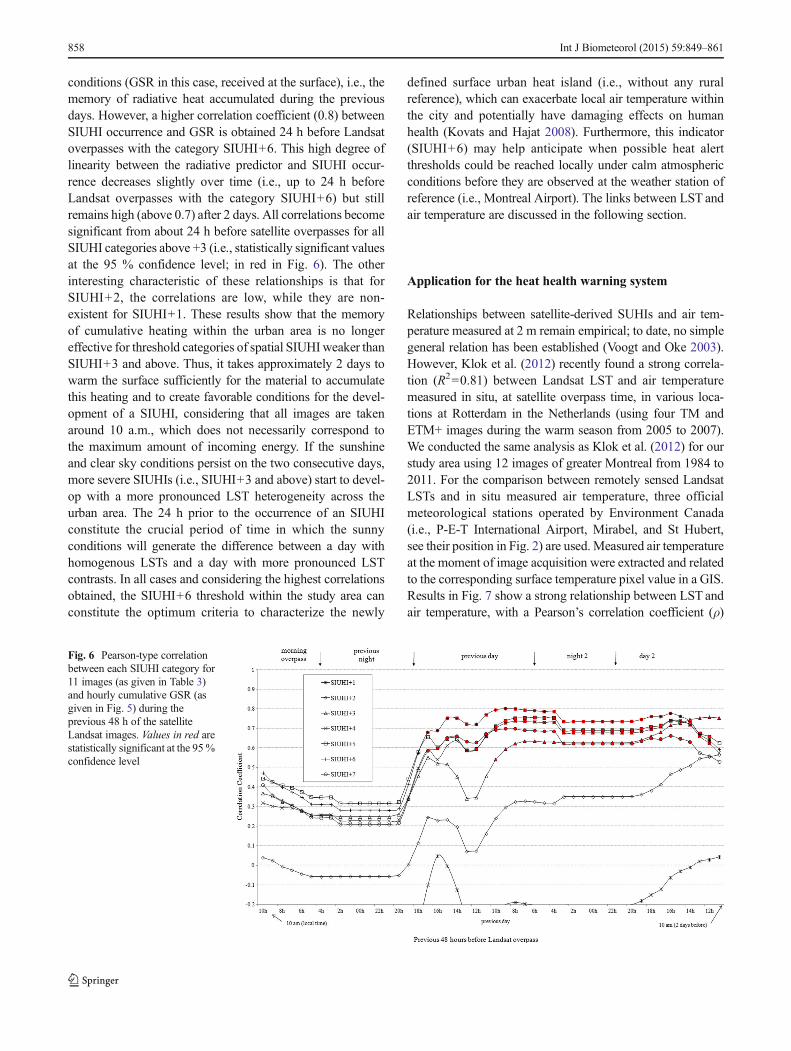
conditions (GSR in this case, received at the surface), i.e., thememory of radiative heat accumulated during the previousdays. However, a higher correlation coefficient (0.8) betweenSIUHI occurrence and GSR is obtained 24 h before Landsatoverpasses with the category SIUHI+6. This high degree oflinearity between the radiative predictor and SIUHI occur-rence decreases slightly over time (i.e., up to 24 h beforeLandsat overpasses with the category SIUHI+6) but stillremains high (above 0.7) after 2 days. All correlations becomesignificant from about 24 h before satellite overpasses for allSIUHI categories above +3 (i.e., statistically significant valuesat the 95 % confidence level; in red in Fig. 6). The otherinteresting characteristic of these relationships is that forSIUHI+2, the correlations are low, while they are non-existent for SIUHI+1. These results show that the memoryof cumulative heating within the urban area is no longereffective for threshold categories of spatial SIUHIweaker thanSIUHI+3 and above. Thus, it takes approximately 2 days towarm the surface sufficiently for the material to accumulatethis heating and to create favorable conditions for the devel-opment of a SIUHI, considering that all images are takenaround 10 a.m., which does not necessarily correspond tothe maximum amount of incoming energy. If the sunshineand clear sky conditions persist on the two consecutive days,more severe SIUHIs (i.e., SIUHI+3 and above) start to devel-op with a more pronounced LST heterogeneity across theurban area. The 24 h prior to the occurrence of an SIUHIconstitute the crucial period of time in which the sunnyconditions will generate the difference between a day withhomogenous LSTs and a day with more pronounced LSTcontrasts. In all cases and considering the highest correlationsobtained, the SIUHI+6 threshold within the study area canconstitute the optimum criteria to characterize the newly

defined surface urban heat island (i.e., without any ruralreference), which can exacerbate local air temperature withinthe city and potentially have damaging effects on humanhealth (Kovats and Hajat 2008). Furthermore, this indicator(SIUHI+6) may help anticipate when possible heat alertthresholds could be reached locally under calm atmosphericconditions before they are observed at the weather station ofreference (i.e., Montreal Airport). The links between LST andair temperature are discussed in the following section.

Application for the heat health warning system

Relationships between satellite-derived SUHIs and air tem-perature measured at 2 m remain empirical; to date, no simplegeneral relation has been established (Voogt and Oke 2003).However, Klok et al. (2012) recently found a strong correla-tion (R2=0.81) between Landsat LST and air temperaturemeasured in situ, at satellite overpass time, in various loca-tions at Rotterdam in the Netherlands (using four TM andETM+ images during the warm season from 2005 to 2007).We conducted the same analysis as Klok et al. (2012) for ourstudy area using 12 images of greater Montreal from 1984 to2011. For the comparison between remotely sensed LandsatLSTs and in situ measured air temperature, three officialmeteorological stations operated by Environment Canada(i.e., P-E-T International Airport, Mirabel, and St Hubert,see their position in Fig. 2) are used. Measured air temperatureat the moment of image acquisition were extracted and relatedto the corresponding surface temperature pixel value in a GIS.Results in Fig. 7 show a strong relationship between LST andair temperature, with a Pearson’s correlation coefficient (ρ)

Fig. 6 Pearson-type correlationbetween each SIUHI category for11 images (as given in Table 3)and hourly cumulative GSR (asgiven in Fig. 5) during theprevious 48 h of the satelliteLandsat images. Values in red arestatistically significant at the 95%confidence level

858 Int J Biometeorol (2015) 59:849–861

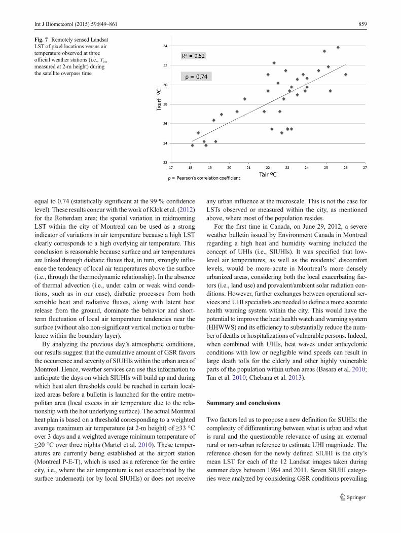
equal to 0.74 (statistically significant at the 99 % confidencelevel). These results concur with the work of Klok et al. (2012)for the Rotterdam area; the spatial variation in midmorningLST within the city of Montreal can be used as a strongindicator of variations in air temperature because a high LSTclearly corresponds to a high overlying air temperature. Thisconclusion is reasonable because surface and air temperaturesare linked through diabatic fluxes that, in turn, strongly influ-ence the tendency of local air temperatures above the surface(i.e., through the thermodynamic relationship). In the absenceof thermal advection (i.e., under calm or weak wind condi-tions, such as in our case), diabatic processes from bothsensible heat and radiative fluxes, along with latent heatrelease from the ground, dominate the behavior and short-term fluctuation of local air temperature tendencies near thesurface (without also non-significant vertical motion or turbu-lence within the boundary layer).

By analyzing the previous day’s atmospheric conditions,our results suggest that the cumulative amount of GSR favorsthe occurrence and severity of SIUHIs within the urban area ofMontreal. Hence, weather services can use this information toanticipate the days on which SIUHIs will build up and duringwhich heat alert thresholds could be reached in certain local-ized areas before a bulletin is launched for the entire metro-politan area (local excess in air temperature due to the rela-tionship with the hot underlying surface). The actual Montrealheat plan is based on a threshold corresponding to a weightedaverage maximum air temperature (at 2-m height) of ≥33 °Cover 3 days and a weighted average minimum temperature of≥20 °C over three nights (Martel et al. 2010). These temper-atures are currently being established at the airport station(Montreal P-E-T), which is used as a reference for the entirecity, i.e., where the air temperature is not exacerbated by thesurface underneath (or by local SIUHIs) or does not receive

any urban influence at the microscale. This is not the case forLSTs observed or measured within the city, as mentionedabove, where most of the population resides.

For the first time in Canada, on June 29, 2012, a severeweather bulletin issued by Environment Canada in Montrealregarding a high heat and humidity warning included theconcept of UHIs (i.e., SIUHIs). It was specified that low-level air temperatures, as well as the residents’ discomfortlevels, would be more acute in Montreal’s more denselyurbanized areas, considering both the local exacerbating fac-tors (i.e., land use) and prevalent/ambient solar radiation con-ditions. However, further exchanges between operational ser-vices and UHI specialists are needed to define a more accuratehealth warning system within the city. This would have thepotential to improve the heat health watch and warning system(HHWWS) and its efficiency to substantially reduce the num-ber of deaths or hospitalizations of vulnerable persons. Indeed,when combined with UHIs, heat waves under anticyclonicconditions with low or negligible wind speeds can result inlarge death tolls for the elderly and other highly vulnerableparts of the population within urban areas (Basara et al. 2010;Tan et al. 2010; Chebana et al. 2013).

Summary and conclusions

Two factors led us to propose a new definition for SUHIs: thecomplexity of differentiating between what is urban and whatis rural and the questionable relevance of using an externalrural or non-urban reference to estimate UHI magnitude. Thereference chosen for the newly defined SIUHI is the city’smean LST for each of the 12 Landsat images taken duringsummer days between 1984 and 2011. Seven SIUHI catego-ries were analyzed by considering GSR conditions prevailing

Fig. 7 Remotely sensed LandsatLST of pixel locations versus airtemperature observed at threeofficial weather stations (i.e., Tairmeasured at 2-m height) duringthe satellite overpass time

Int J Biometeorol (2015) 59:849–861 859

prior to and during each acquisition date. The results revealedthat cumulative GSR during the 2 days prior to acquisition ofthe image is a relevant predictor contributing to higher heatabsorption in urban landscapes and influencing the occurrenceand severity of SIUHIs (the highest correlation found on theprevious day). The threshold of 6 °C above the city’s meanLST was found to be the optimum criterion among otherthresholds to identify the newly proposed SIUHI. In 25 years,or between 1984 and 2008, the spread of SIUHI+6 hasincreased by 63 % (or from 48.7 to 79.5 km2).

Our suggested method for defining SIUHIs could be repli-cated in other areas around the globe for which satellite andmeteorological data are available. It is probable that the SIUHIthreshold might be different for other cities with differentsatellite overpass times, sensors (Landsat 8, launched inFebruary 2013), land use, or during another season.However, as a UHI is a relative measure that takes intoaccount local physiographic and atmospheric conditions, theassessment of a hotspot (SIUHI) within a particular city needsto account for the cumulative effect of ambient and prevalentGSR as well as other meteorological conditions that couldexacerbate local surface and air temperature conditions. Asexperienced in various cities across the world, the effects ofSUHIs (SIUHIs in our case) have been successfully mitigated,as those have been clearly identified, by increasing urbanvegetation and green spaces and by installing green roofs onthe tops of buildings (Bass et al. 2002; Rosenzweig et al.2006; Oberndorfer et al. 2007). Klok et al. (2012) found thata 10 % increase in green area decreased the surface tempera-ture by 1.3 °C for the city of Rotterdam in the Netherlands.

The SIUHI+6 can not only be considered as a local thresh-old for Montreal for identifying hotspots within the city butalso be used as an important criterion to consider within anHHWWS. For example, Environment Canada’s meteorologi-cal services (Meteorological Service of Canada (MSC)) hasused this criterion to better define and locate Montreal’shottest areas during a heat spell and to determine where thehelp and intervention by public health services may need to beprioritized. The MSC is implementing a 2-year measurementcampaign of air temperature within the urban core ofMontrealduring the 2013 and 2014 summer seasons. These campaignsare conducted using 30 sites identified on the basis of theirspecific fraction of vegetation and land cover. In the firstphase, data from the sites will provide estimates of recurrentdifferences between the air temperature observed at the airportand air temperature observed in different areas within the city.Subsequent analysis will lead us to improve heat warningsystems through spatial screening, allowing for timely warn-ings to be issued to the most vulnerable areas during a hotspell event. The threshold of 33 °C (over 3 days) can bereached in a residential area before it is reached at the airportor elsewhere in the city (SIUHI effects). In the second phase, acomparison will be made between LST and in situ measured

air temperature to further analyze the relationship betweenboth (surface and air) temperatures, based on the variousurban materials and on the previous and ambient atmosphericconditions. This will help to further evaluate if the consideredeffects of ambient and prevalent GSR conditions on SIUHIthresholds induce similar behaviors on air temperature withinthe city, especially in terms of intensity and occurrence of thehottest conditions.

Acknowledgments This work was funded by the Climate ChangeAction Fund (CCAF) program of the federal government, the ConseilRégional de l’Environnement de Laval (CREL), and the City ofMontreal.Support of this research by the Department of Geography, Université duQuébec à Montréal (UQÀM), and Environment Canada is gratefullyacknowledged. We would also like to thank Michelle Marchant, RabahAider, and Christian Saad for their technical support, as well as SergeMainville, Gilles Morneau, Didier Davignon, Gilles Simard, StéphaneGagnon, and Marc Beauchemin from Environment Canada for theirconstructive comments and discussion. The authors would also like tothank the DAI team for providing the data and technical support. TheDAIportal (http://loki.qc.ec.gc.ca/DAI/DAI-f.html) is made possible throughcollaboration among the Global Environmental and Climate ChangeCentre (GEC3), the Adaptation and Impacts Research Division (AIRD)of Environment Canada, and the Drought Research Initiative (DRI).

Open Access This article is distributed under the terms of the CreativeCommons Attribution License which permits any use, distribution, andreproduction in any medium, provided the original author(s) and thesource are credited.

References

Allen RG, Tasumi M, Trezza R, Bastiaanssen WGM (2002) SurfaceEnergy Balance Algorithm for Land (SEBAL). Advanced trainingand user’s manual, University of Idaho, Kimberly, ID, p 98

Badarinath KVS, Kiran Chand TR, Madhavi Lathaand K,Raghavaswamy V (2005) Studies on urban heat islands usingEnvisat AATSR data. J Indian Soc Remote Sens 33(4):495–501

Basara JB, Basara HG, Illston BG, Crawford KC (2010) The impact ofthe urban heat island during an intense heat wave in Oklahoma City.Adv Meteorol 2010, 230365. doi:10.1155/2010/230365

Bass B, Krayenhoff S, Martilli A (2002) Mitigating the urban heat islandwith green roof infrastructure. Urban Heat Island Summit, Toronto

Carnahan WH, Larson RC (1990) An analysis of an urban heat sink.Remote Sens Environ 33:65–71

Chebana F, Martel B, Gosselin P, Giroux JX, Ouarda TBMJ (2013) Ageneral and flexible methodology to define thresholds for heathealth watch and warning systems, applied to the province ofQuebec (Canada). Int J Biometeorol 57(4):631–644. doi:10.1007/s00484-012-0590-2

Clarke JF (1972) Some effects of the urban structure on heat mortality.Environ Res 5:93–104

Duffie JA, Beckman WA (1980) Solar engineering of thermal processes.John Wiley and Sons, New York, pp 1–109

Faris AA, Sudhakar Reddy Y (2010) Estimation of urban heat Islandusing Landsat-7 ETM+ imagery at Chennai city - a case study. Int JEarth Sci Eng 3(3):332–340

Hafner J, Kidder SQ (1999) Urban heat island modeling in conjunctionwith satellite-derived surface/soil parameters. J Appl Meteorol 38:448–465

860 Int J Biometeorol (2015) 59:849–861

Hoffmann P, Krueger O, Heinke K (2011) A statistical model for theurban heat island and its application to a climate change scenario. IntJ Climatol. doi:10.1002/joc.2348

Hupfer P, Kuttler W (2006) In: B. G. Teubner Verlag/GWV (ed) Weatherand climate: an introduction to meteorology and climatology.GmbH, Wiesbaden, p 554

Imhoff ML, Zhang P, Wolfe RE, Bounoua L (2010) Remote sensing ofthe urban heat island effect across biomes in the continental USA.Remote Sens Environ 114(3):504–513

Jiang Z, Chen Y, Li J (2006) On urban heat island of Beijing based onLandsat TM data. Geo Spat Inf Sci 9(4):293–297

Kawai T, Kanda M (2010) Urban energy balance obtained from thecomprehensive outdoor scale model experiment. Part I: basic fea-tures of the surface energy balance. J Appl Meteorol Climatol 49:1341–1359

Kim YH (1992) Urban heat island. Int J Remote Sens 13(12):2319–2336Klok L, Zwart S, Verhagen H, Mauri E (2012) The surface heat island of

Rotterdam and its relationship with urban surface characteristics.Resour Conserv Recycl 64:23–29

Kovats RS, Hajat S (2008) Heat stress and public health: a critical review.Annu Rev Public Health 29:41–55

Lee L, Chen L,WangX, Zhao J (2011) Use of Landsat TM/ETM+ data toanalyze urban heat island and its relationship with land use/coverchange. International Conference on Remote Sensing, Environmentand Transportation Engineering (RSETE), IEEE, Nanjing, 24–26June 2011, p 922–927

Lowry WP (1977) Empirical estimation of the urban effects on climate: aproblem analysis. J Appl Meteorol 16:129–135

Martel B, Giroux JX, Gosselin P, Chebana F, Ouarda TBMJ, Charron C(2010) Indicateurs et seuils météorologiques pour les systèmes deveille-avertissement lors de vagues de chaleur au Québec. InstitutNational de Santé publique du Québec

Oberndorfer E, Lundholm J, Bass B, Coffman RR, Doshi H, Dunnett N,Gaffin S, Kohler M, Liu KKY, Rowe B (2007) Green roofs as urbanecosystems: ecological structures, functions, and services.Bioscience 57:823–833

Oke TR (1976) The distinction between canopy and boundary-layer heatislands. Atmosphere 14:268–277

Oke TR (1982) The energetic basis of the urban heat island. Q J RMeteorol Soc 108:1–24

Oke TR (1987) Boundary layer climates, 2nd edition. Routledge, Taylorand Francis Group, Cambridge, p 435

Oke TR (1997) Urban climates and global change. In: Perry A,Thompson R (eds) Applied climatology: principles and practices.Routledge, London, pp 273–287

Oke TR (2004) Initial guidance to obtain representative meteorologicalobservations at urban sites. IOM Report 81, World MeteorologicalOrganization, Geneva

Oke TR (2009) The need to establish protocols in urban heat island work.Paper presented at the T. R. Oke Symposium & Eighth Symposiumon Urban Environment, 11–15 January, Phoenix. URL http://ams.confex.com/ams/89annual/techprogram/paper150552.htm.Accessed 26 June 2012

Parlow E (1999) Remotely-sensed heat flux of urban areas. In: deDear, et al. (eds) Biometeorology and urban climatology at

the turn of the millennium, WMO Tech. Doc., Vol. 1026. (p.523–528). Geneva, Switzerland: World MeteorologicalOrganization

Rigo G, Zech L, Parlow E (2003) Validation of satellite longwaveemission with in-situ measurement during Bubble. Proc. 5thICUC, Sept. 2003, Lodz Poland, vol. 2, 359–366

Rooney CAJM, Kovats RS, Coleman MP (1998) Excess mortalityin England and Wales, and in Greater London, during the1995 heatwave. J Epidemiol Community Health 52:482–486

Rosenzweig C, Solecki WD, Slosberg R (2006) Mitigating New YorkCity’s heat island with urban forestry, living roofs, and light sur-faces. A report to the New York State Energy Research andDevelopment Authority

Roth M, Oke TR, Emery WJ (1989) Satellite derived urban heat islandsfrom three coastal cities and the utilization of such data in urbanclimatology. Int J Remote Sens 10:1699–1720

Runnalls KE, Oke TR (2000) Dynamics and controls of Vancouver’snear-surface urban heat island. Phys Geogr 21:283–304

Shepherd MJ (2006) Evidence of urban-induced precipitation variabilityin arid climate regimes. J Arid Environ 67(4):607–628

Singh NK, Bajwa SG (2007) Analysis of evolving surface urban heatisland in NWArkansas. IEEE Region 5 Technical Conference, TPS,art. no. 4380398, p. 409–414

Smargiassi A, Goldberg MS, Plante C, Fournier M, Baudouin Y,Kosatsky T (2009) Variation of daily warm season mortality as afunction of micro-urban heat islands. J Epidemiol CommunityHealth 63:659–664

Stewart ID (2011) A systematic review and scientific critique of method-ology in modern urban heat island literature. Int J Climatol 31(2):200–217

Stewart ID, Oke TR (2006) Methodological concerns surrounding theclassification of urban and rural climate stations to define urban heatisland magnitude. Preprints, 6th Int. Conf. on Urban Climate,Goteborg, Sweden

Stewart ID, Oke TR (2009a) Newly developed “thermal climate zones”for defining and measuring urban heat island magnitude in thecanopy layer. Preprints, Oke T. R., Symposium & EighthSymposium on Urban Environment, January 11–15, Phoenix, AZ

Stewart ID, Oke TR (2009b) Classifying urban climate field sites by“local climate zones”: The case of Nagano, Japan. Preprints,Seventh International Conference on Urban Climate, June 29-July3, Yokohama, Japan

Streutker DR (2002) A remote sensing study of the urban heat island ofHouston, Texas. Int J Remote Sens 23(13):2595–2608

Tan J, ZhengY, TangX,GupC, Li L, SongG, ZhenX,Yuan D, KalksteinA, Li F (2010) The urban heat island and its impact on heat wavesand human health in Shanghai. Int J Biometeorol 54(1):75–84

Voogt JA, Oke TR (2003) Thermal remote sensing of urban climates.Remote Sens Environ 86:370–384

Weng Q (2001) A remote sensing GIS evaluation of urban expansion andits impact on surface temperature in the Zhujiang Delta, China. Int JRemote Sens 22:1999–2014

Xian G, Crane M (2006) An analysis of urban thermal characteristics andassociated land cover in Tampa Bay and Las Vegas using Landsatsatellite data. Remote Sens Environ 104(2):147–156

Int J Biometeorol (2015) 59:849–861 861