An Alternative Approach

• If you have a sufficient history & the demand is relatively stable over time, then use an empirical distribution

• In the case Sport Obermeyer (Simchi-Levi’s textbook)

An Example • Demand for a Weekly Magazine in the past 52

weeks (Computer Today)

15 19 9 12 9 22 4 7 8 11

14 11 6 11 9 18 10 0 14 12

8 9 5 4 4 17 18 14 15 8

6 7 12 15 15 19 9 10 9 16

8 11 11 18 15 17 19 14 14 17

13 12

Frequency Histogram

0

1

2

3

4

5

6

7

Actual Demand

Weeks

Continuous Distribution

0

1

2

3

4

5

6

7

-6 -4 -2 0 2 4 6 8

10

12

14

16

18

20

22

24

26

28

30

Demand

Fre

quency

73.11D

74.4s

Normal Distribution Parameters (mu, sigma^2):

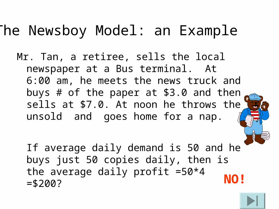
The Newsboy Model: an Example

Mr. Tan, a retiree, sells the local newspaper at a Bus terminal. At 6:00 am, he meets the news truck and buys # of the paper at $3.0 and then sells at $7.0. At noon he throws the unsold and goes home for a nap.

If average daily demand is 50 and he buys just 50 copies daily, then is the average daily profit =50*4 =$200?

NO!

The Intuition

• There is a tradeoff between ordering too much and ordering too little

• To balance these forces, it’s useful to think in terms of a cost for ordering too much and a cost for ordering too little – A cost here can be a loss of profit

• Overstocking cost C0

= loss incurred when a unit unsold at end of selling season

• Understocking cost Cu

= profit margin lost due to lost sale (because no inventory on hand)

In the example: C0 = -3, Cu = 4

Deriving the Formula: Critical Ratio

Increase order from k to k+1 if Prob(Demand < k) < 4

3 + 4

Order k+1 instead of k if4*P(d k+1)P(d<k) > 0

or 4*[1-P(d<k)] - 3*P(d< k ) > 0

order k+1

keep order size at k

instead of k

1 more unsold

1 fewer lost sale

-3 =Co

P(d k+1)

P(d<k)

Cu

Additional contribution

=0.57

Let P(d<=k) = Prob (d <= k)

Newsvendor Model-Demand Distribution Continuous

Order Q such that

Prob(Demand < Q) = Cu

Co + Cu

QCritical ratio r(Q)

z 0.00 0.01 0.02 0.03 0.04 0.05 0.06 0.07 0.08 0.090.0 0.5000 0.5040 0.5080 0.5120 0.5160 0.5199 0.5239 0.5279 0.5319 0.53590.1 0.5398 0.5438 0.5478 0.5517 0.5557 0.5596 0.5636 0.5675 0.5714 0.57530.2 0.5793 0.5832 0.5871 0.5910 0.5948 0.5987 0.6026 0.6064 0.6103 0.61410.3 0.6179 0.6217 0.6255 0.6293 0.6331 0.6368 0.6406 0.6443 0.6480 0.65170.4 0.6554 0.6591 0.6628 0.6664 0.6700 0.6736 0.6772 0.6808 0.6844 0.68790.5 0.6915 0.6950 0.6985 0.7019 0.7054 0.7088 0.7123 0.7157 0.7190 0.72240.6 0.7257 0.7291 0.7324 0.7357 0.7389 0.7422 0.7454 0.7486 0.7517 0.75490.7 0.7580 0.7611 0.7642 0.7673 0.7704 0.7734 0.7764 0.7794 0.7823 0.78520.8 0.7881 0.7910 0.7939 0.7967 0.7995 0.8023 0.8051 0.8078 0.8106 0.81330.9 0.8159 0.8186 0.8212 0.8238 0.8264 0.8289 0.8315 0.8340 0.8365 0.83891.0 0.8413 0.8438 0.8461 0.8485 0.8508 0.8531 0.8554 0.8577 0.8599 0.86211.1 0.8643 0.8665 0.8686 0.8708 0.8729 0.8749 0.8770 0.8790 0.8810 0.88301.2 0.8849 0.8869 0.8888 0.8907 0.8925 0.8944 0.8962 0.8980 0.8997 0.90151.3 0.9032 0.9049 0.9066 0.9082 0.9099 0.9115 0.9131 0.9147 0.9162 0.91771.4 0.9192 0.9207 0.9222 0.9236 0.9251 0.9265 0.9279 0.9292 0.9306 0.93191.5 0.9332 0.9345 0.9357 0.9370 0.9382 0.9394 0.9406 0.9418 0.9429 0.94411.6 0.9452 0.9463 0.9474 0.9484 0.9495 0.9505 0.9515 0.9525 0.9535 0.95451.7 0.9554 0.9564 0.9573 0.9582 0.9591 0.9599 0.9608 0.9616 0.9625 0.96331.8 0.9641 0.9649 0.9656 0.9664 0.9671 0.9678 0.9686 0.9693 0.9699 0.97061.9 0.9713 0.9719 0.9726 0.9732 0.9738 0.9744 0.9750 0.9756 0.9761 0.97672.0 0.9772 0.9778 0.9783 0.9788 0.9793 0.9798 0.9803 0.9808 0.9812 0.98172.1 0.9821 0.9826 0.9830 0.9834 0.9838 0.9842 0.9846 0.9850 0.9854 0.98572.2 0.9861 0.9864 0.9868 0.9871 0.9875 0.9878 0.9881 0.9884 0.9887 0.98902.3 0.9893 0.9896 0.9898 0.9901 0.9904 0.9906 0.9909 0.9911 0.9913 0.99162.4 0.9918 0.9920 0.9922 0.9925 0.9927 0.9929 0.9931 0.9932 0.9934 0.99362.5 0.9938 0.9940 0.9941 0.9943 0.9945 0.9946 0.9948 0.9949 0.9951 0.99522.6 0.9953 0.9955 0.9956 0.9957 0.9959 0.9960 0.9961 0.9962 0.9963 0.99642.7 0.9965 0.9966 0.9967 0.9968 0.9969 0.9970 0.9971 0.9972 0.9973 0.99742.8 0.9974 0.9975 0.9976 0.9977 0.9977 0.9978 0.9979 0.9979 0.9980 0.99812.9 0.9981 0.9982 0.9982 0.9983 0.9984 0.9984 0.9985 0.9985 0.9986 0.99863.0 0.9987 0.9987 0.9987 0.9988 0.9988 0.9989 0.9989 0.9989 0.9990 0.99903.1 0.9990 0.9991 0.9991 0.9991 0.9992 0.9992 0.9992 0.9992 0.9993 0.99933.2 0.9993 0.9993 0.9994 0.9994 0.9994 0.9994 0.9994 0.9995 0.9995 0.99953.3 0.9995 0.9995 0.9995 0.9996 0.9996 0.9996 0.9996 0.9996 0.9996 0.9997

F(z)

0 z

Normal Dist. If F* = 0.65, z = 0.385

Q*=aver.+z*stdev

If F* =0.45, z= -0.125

Q* = aver. + z*stdev

If F* = 0.65, z = 0.385

Q*=100 +0.385*20

If F* =0.45, z= -0.125

Q* = 100 – 0.125*20

• Purchasing cost $0.25/per copy ， selling price =$ 0.75 。 If unsold after the week, each copy can be salvaged at $0.1 (to be returned to the publisher) 。 What’s the optimal order quantity Q?

• F(Q) = 15.010.025.0 oc50.025.075.0 uc

77.050.015.0

50.0)( *

QF

•

• From the previous normal table ， z=0.74 。 Thus optimal weekly order quantity

16or 1524.1574.474.073.11* Q

*Q

Area=0.77

demand， d

f(x)

74.4

73.11

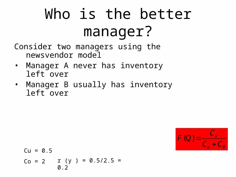
Who is the better manager?

Consider two managers using the newsvendor model

• Manager A never has inventory left over• Manager B usually has inventory left over

Cu = 0.5

Co = 2 r (y ) = 0.5/2.5 = 0.2

0

)(CC

CQF

u

u

Who is the better manager?

Consider two managers using the newsvendor model

• Manager A never has inventory left over• Manager B usually has inventory left over

What if they both sell Valentine’s cards:

Cu=$2.00

Co=$0.20 r (Q) = 2/2.2 = 0.91

Cu = 0.5

Co = 2 r (y ) = 0.5/2.5 = 0.2

0u

u

CC

C)Q(r

END