An Algorithm to Simplify Tensor Expressions

R. Portugal1

Department of Applied Mathematics, University of Waterloo, Waterloo, Ontario, N2L 3G1 - Canada.

Abstract

The problem of simplifying tensor expressions is addressed in two parts. The first part presentsan algorithm designed to put tensor expressions into a canonical form, taking into account thesymmetries with respect to index permutations and the renaming of dummy indices. The tensorindices are split into classes and a natural place for them is defined. The canonical form is theclosest configuration to the natural configuration. In the second part, the Grobner basis method isused to simplify tensor expressions which obey the linear identities that come from cyclic symmetries(or more general tensor identities, including non-linear identities). The algorithm is suitable forimplementation in general purpose computer algebra systems. Some timings of an experimentalimplementation over the Riemann package are shown.

1 Introduction

Recently, some attempts to describe algorithms for simplifying tensor expressions have appeared inthe literature.[1][2][3] The tensor symmetry properties and the presence of dummy indices make theproblem complex. Fulling et al.[1] described an algorithm to enumerate the independent monomi-als built from the Riemann tensor and its covariant derivative. They presented explicit tables formonomials of order 12 or less in derivatives of the metric. Although explicit bases are presented formonomial of order 8 or less, they have not described neither a systematic algorithm to build the basisnor a method to simplify generic tensor expressions built using the Riemann tensor. Using the samealgorithm, Wybourne and Meller[4] enumerated the order-14 invariants. On the other hand, Ilyinand Kryukov[2] did present an algorithm to simplify general tensor expressions based on the groupalgebra of the permutation group. Though the method is elegant from the mathematical point ofview, it is inefficient. Quoting the authors: “hardware development is very fast now, and it will bepossible to solve problems with 11 indices with the help of our program”. Dresse presented in thesecond part of his PhD dissertation[3] a new algorithm to simplify tensor expression based on thebacktrack algorithms for combinatorial objects.[5] Most of his effort has been directed to solve the“dummy index problem” (described bellow).

In this work, the problem is addressed in two parts. In the first, the tensor expressions areput into a canonical form taking into account the symmetries with respect to index permutations

1On leave from Centro Brasileiro de Pesquisas Fısicas, Rua Dr. Xavier Sigaud 150, Urca, Rio de Janeiro, Brazil.CEP 22290-180. Email: portugal@cat.cbpf.br

1

and renaming of dummy indices. In the second part, the Grobner basis method (see Geddes atal.[6] and refs. therein) is used to address the linear identities that come from cyclic symmetries(or more general tensor identities). The algorithm is suitable for implementation in general purposecomputer algebra systems, since many functionalities of these systems (besides the Grobner basisimplementation) are required.

It is known that the names of the dummy indices have no intrinsic meaning, and the presence oftwo or more of them in a tensor expression creates symmetries with respect to renaming. This leadsto algorithms of complexity O(n!) where n is the number of dummy indices. Dummy indices difficultthe definition of tensor rules and the use of pattern matching. One way to solve the dummy indexproblem is to rename them in terms of the index positions and the name of the tensors (see step 9of the algorithm). However, the tensor symmetries may change the index positions, invalidating theprocess. This kind of renaming method is invariant if there is a prescribed method to put the indicesinto a canonical position.

In section 2, an algorithm to put tensor expressions into a canonical form is described. Thecanonical position of the indices is based on definitions 3 to 6. Some parts of the definitions of thissection involve conventions that can be changed without losing the “canonicalization” character ofthe algorithm. The ideal format for the canonical tensor is

T F+ SII A+ B+ C+ SI

C− B− A− F−

where F+, SII , A+, B+, C+, SI , C−, B−, A− and F− represent sequences of indices whose meanings

are defined in step 7 of the algorithm. The indices of class SI can have contravariant or covariantcharacter. They are placed in the midst of the classes that have the character fixed. This idealformat is only achieved in special cases, as when the tensor T is totally symmetric or antisymmetric.The canonical position of the indices is the one closest to this format, where the notion of “closest”is precisely defined.

Product of equal tensors is addressed by reduction to one tensor of rank equal to the sum of therank of the factors. This reduction process is used in other parts of the algorithm in order to simplifythe implementation.

In section 3, some timings of an experimental implementation of the algorithm over the Riemannpackage[7] are presented. Polynomials built from the Riemann tensor are challenges for any algorithmto simplify tensor expressions. I believe that special techniques can improve the timings for the kindof symmetries of the Riemann tensor, but none has been implemented for the demonstration of thissection. The implementation in the Maple system[8] can easely handle products of three Riemanntensors.

In section 4, the problem of the simplification of tensor expressions under the presence of sidetensor identities, which come generally from cyclic symmetries, is addressed. The Grobner basisimplementation of the Maple system is used to accomplish the full simplification.

2 The algorithm

Consider the definition of the normal and canonical functions given in Geddes et al.[6] Let A be a setof algebraic expressions which admits a canonical function. Consider the operations of multiplication,addition and contraction of tensors as defined in the tensor algebra.[9][10][11] If a coordinate systemhas been selected, the tensor algebra can be performed through the tensor components. In this work,

2

a tensor expression is any expression written in terms of non-assigned tensor components obeying therules of the tensor algebra whose coefficient factors are members of the set A. Consider Riemannianspaces, in which exists a fundamental metric tensor which establish a relation between the covariantand contravariant tensor indices.

2.1 Definitions

Hypothesis 1: Tensors do not obey any side tensor identities except symmetries with respect toindex permutations or symmetries with respect to renaming or the inversion of character of dummyindices.

“Symmetries with respect to index permutations” means that the tensors obey one or moreequations of the kind

T i1 ··· in = ε T π(i1 ··· in),

where ε = 1 or ε = − 1 and π(i1 · · · in) is any permutation of i1 · · · in.

Definition 1: Induced symmetry of a sub-set of indices of a tensor.The induced symmetries of a sub-set of indices of a tensor are the symmetries that the sub-set

inherits from the symmetries of the whole set of indices. Pairs of dummy indices are treated asindependent free indices, hence not permutable.

For example, the induced symmetry of the first two indices of the Riemann tensor is the skewsymmetry. The second and third indices have no induced symmetry regardless any contractionbetween the first and fourth indices.

Definition 2: Equivalent index configurations.Two index configurations2 of a tensor T extracted from a tensor product are said to be equivalent

if one configuration can be put into the other by the use of any of the following properties:1. Character inversion of the dummy indices,2. Renaming the dummy indices,3. Index permutation allowed by the symmetries of the tensors of the tensor product.

Definition 3: Suppose the tensor T has n indices and let (λ1, · · ·, λp) be a partition of n wherep is a positive integer less or equal than n. The indices of T can be grouped in disjoint classesC1, · · ·, Cp where a generic class Ci has λi indices. The indices of each class can be substitutedwith numbers in such way that the indices of class Ci run from (

∑i−1j=1 λj) + 1 to

∑ij=1 λj . Consider

all index configurations of the tensor T and let the indices be substituted with the correspondingnumbers. The configurations are in one-to-one correspondence with the elements of the symmetricgroup Sn.[12][13] The following criteria establish an order of decreasing configurations with respectto classes C1 to Cp:

a. Smaller value of the position of the first index of class C1 in the tensor T . If the positions areequal, consider the position of the next index of class C1. If the positions of all indices of class C1

are equal, consider the positions of the indices of the next classes until Cp.

2The index configuration is the list of indices of the tensor, taking into account the character of each index.

3

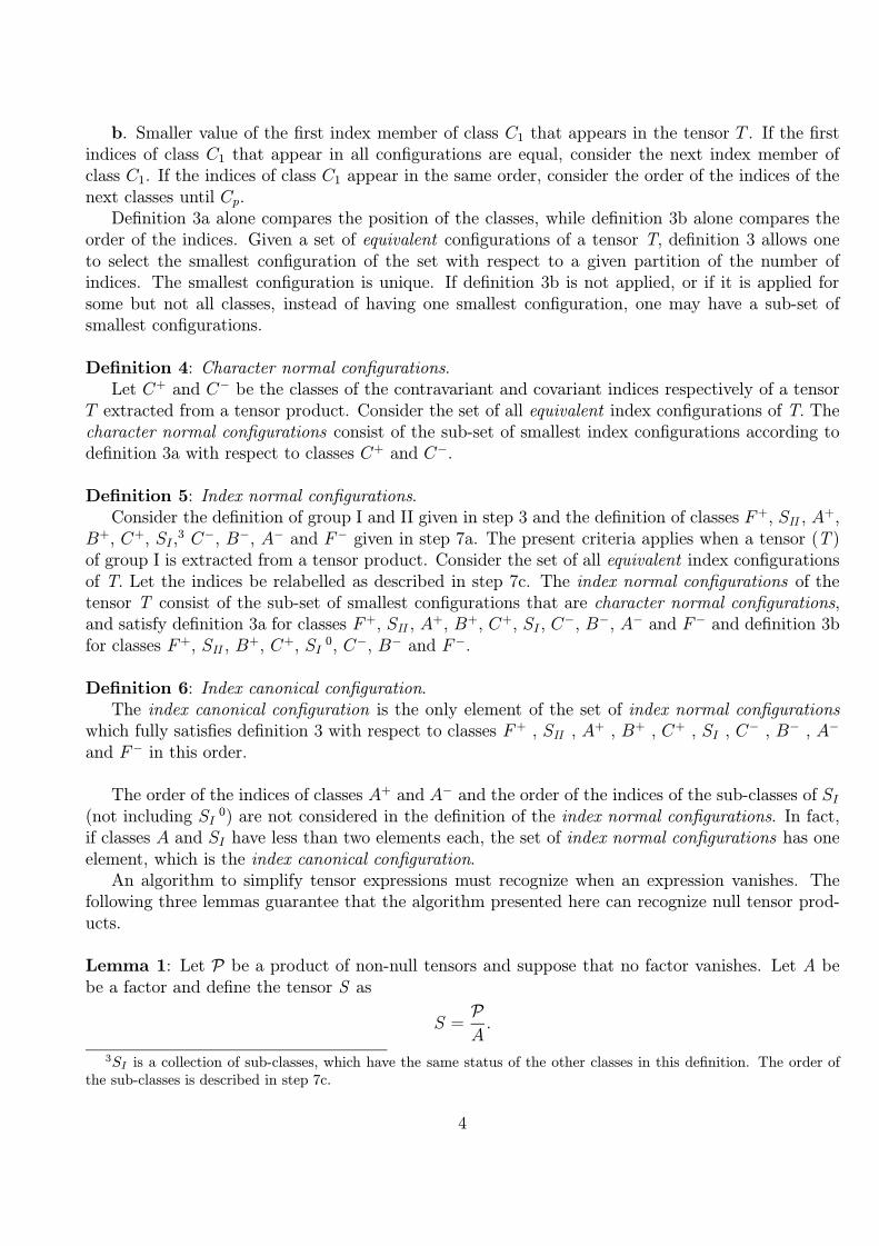
b. Smaller value of the first index member of class C1 that appears in the tensor T . If the firstindices of class C1 that appear in all configurations are equal, consider the next index member ofclass C1. If the indices of class C1 appear in the same order, consider the order of the indices of thenext classes until Cp.

Definition 3a alone compares the position of the classes, while definition 3b alone compares theorder of the indices. Given a set of equivalent configurations of a tensor T, definition 3 allows oneto select the smallest configuration of the set with respect to a given partition of the number ofindices. The smallest configuration is unique. If definition 3b is not applied, or if it is applied forsome but not all classes, instead of having one smallest configuration, one may have a sub-set ofsmallest configurations.

Definition 4: Character normal configurations.Let C+ and C− be the classes of the contravariant and covariant indices respectively of a tensor

T extracted from a tensor product. Consider the set of all equivalent index configurations of T. Thecharacter normal configurations consist of the sub-set of smallest index configurations according todefinition 3a with respect to classes C+ and C−.

Definition 5: Index normal configurations.Consider the definition of group I and II given in step 3 and the definition of classes F+, SII , A+,

B+, C+, SI ,3 C−, B−, A− and F− given in step 7a. The present criteria applies when a tensor (T )

of group I is extracted from a tensor product. Consider the set of all equivalent index configurationsof T. Let the indices be relabelled as described in step 7c. The index normal configurations of thetensor T consist of the sub-set of smallest configurations that are character normal configurations,and satisfy definition 3a for classes F+, SII , A+, B+, C+, SI , C

−, B−, A− and F− and definition 3bfor classes F+, SII , B+, C+, SI

0, C−, B− and F−.

Definition 6: Index canonical configuration.The index canonical configuration is the only element of the set of index normal configurations

which fully satisfies definition 3 with respect to classes F+ , SII , A+ , B+ , C+ , SI , C− , B− , A−

and F− in this order.

The order of the indices of classes A+ and A− and the order of the indices of the sub-classes of SI(not including SI

0) are not considered in the definition of the index normal configurations. In fact,if classes A and SI have less than two elements each, the set of index normal configurations has oneelement, which is the index canonical configuration.

An algorithm to simplify tensor expressions must recognize when an expression vanishes. Thefollowing three lemmas guarantee that the algorithm presented here can recognize null tensor prod-ucts.

Lemma 1: Let P be a product of non-null tensors and suppose that no factor vanishes. Let A bebe a factor and define the tensor S as

S =P

A.

3SI is a collection of sub-classes, which have the same status of the other classes in this definition. The order ofthe sub-classes is described in step 7c.

4

Suppose that A and S share n contracted indices. Let s be the rank of S, and a be n plus the numberof free indices of A.

The product P is zero if and only if there exists a factor A having the symmetry

A i1 ··· ia = −A π(i1 ··· ia) (1)

where the permutation π acts only on the indices contracted with the indices of S, and P is invariantunder the application of the permutation π on the corresponding indices of S, that is

P = A i1 ··· ia S π(j1 ··· js), (2)

where n j ’s are equal to n i ’s and the permutation π acts on names, not on positions.4 A may haveindices contracted internally which have not been represented in (1) and (2). Symmetry (1) takesaccount of permutations and character inversions of the dummy indices within A.Proof: (⇒)(by reductio ad absurdum) There are two cases:

1. If P is not invariant for any factor A that has the symmetry (1), then

P 6= A i1 ··· ia S π(j1 ··· js).

Using (1) and renaming the dummy indices, it follows that P 6= −P, therefore P 6= 0.2. If no factor admits a symmetry π of the form (1), from the supposition that no factor of P

vanishes, it follows that P 6= 0.

So far only products of non-vanishing factors have been considered. What are the conditions thatcancel a single generic tensor with some or all indices contracted? The answer can be obtained fromlemma 1. Suppose that T is a tensor of rank m with 2n indices contracted. This tensor can bewritten as

g i1j1 · · · g injn Tσ(i1 j1 ··· in jn f1 ··· fm−2n), (3)

where σ is the permutation of i1 j1 · · · in jn f1 · · · fm−2n that specifies the actual order of the indicesof T, and g i j is the metric supposedly symmetric. The free indices are f1 · · · fm−2n. For this case,the tensor S of lemma 1 is

S i1 j1 · · · in jn = g i1j1 · · · g injn,

and is symmetric under the interchange of i pj p into j pi p for p ≤ n, and is totally symmetric underthe pair interchange of i pj p into i qj q for p, q ≤ n. Tensor S does not vanish (again from lemma 1).

If the second factor of (3) does not vanish, there are two cases to consider regarding lemma 1.In the first case, tensor T has antisymmetry (1) while S is symmetric under the same permutationacting on the corresponding indices independently of S being multiplied by T. In the second case,the indices of S has the symmetry (2) only if one considers the contractions of indices between Sand T. These cases reflect items (i) and (ii) respectively of the following lemma.

4The character of the indices of A and S need not be contravariant and covariant respectively. The only restrictionis that the character of the dummy indices are opposite.

5

Lemma 2: Let T be a non-null tensor of rank m with 2n indices contracted (2n ≤ m). Let σ be apermutation such that

T σ(i1 j1 ··· in jn f1 ··· fm−2n) (4)

describes an index configuration with m free indices, such that after j p (p ≤ n) indices are loweredby the metric terms as described in (3), one obtains the actual index positions of T. Suppose that(4) does not vanish. T is zero if and only if at least one of the following items is satisfied.

(i) Consider (4). Independently of any contraction, there is a permutation ρ acting on i1 j1 · · · in jnsuch that

T ρ◦σ(i1 j1 ··· in jn f1 ··· fm−2n) = ε T σ(i1 j1 ··· in jn f1 ··· fm−2n)

where ε = 1 or ε = −1 and at least one of the following items is satisfied.

(i.1) T ρ◦σ(i1 j1 ··· in jn f1 ··· fm−2n) is antisymmetric under one or more interchanges of i pj p into j pi pfor p ≤ n

(i.2) T ρ◦σ(i1 j1 ··· in jn f1 ··· fm−2n) is antisymmetric under one or more pair interchange of i pj p intoi qj q for p, q ≤ n.

(ii) There is an index character configuration such that T is antisymmetric under a permutationπ acting on the contravariant indices (like (1)) and T is invariant under the same permutationacting on the corresponding covariant indices (like (2) with all indices in the same tensor).

Proof: [14]

For example, suppose that T is a tensor of rank 6 with the symmetries

T i j k lmn = −T k l i j mn,

T i j k lmn = T j i k lmn,

T i j k lmn = T i j l kmn,

T i j k lmn = T i j k l nm.

Consider the index configuration

T i k li k l (5)

which is equivalent to zero. Due to the contraction of the first and fourth indices, (5) is antisymmetricunder the interchange of k+ and l+, and is symmetric under the interchange of k− and l−. This isan example of item (ii) of lemma 2.

There is one case not analyzed yet. A tensor T may vanish due to symmetries regardless of anyindex contraction. This case has no practical applications but the algorithm must recognize what arethe combinations of symmetries that cancel the tensor. That recognition can be done at the momentof defining the tensor, before the algorithm is executed. From now on, suppose that tensors are notzero if there is no index contraction.

Let M be the set of all mathematically equivalent tensor products generated by all possibleequivalent configurations of the indices of the tensors of P (P is a product of non-null tensors when

6

all indices are considered free). Definitions 4-6 can be extended to products of tensors by applicationon each factor.

Lemma 3: Two elements of M have the index canonical configuration with opposite signs if andonly if P is zero.Proof : (⇒) If P is mathematically equivalent to P’ and −P’ simultaneously then P = 0.

(⇐) If P is zero, either one of the factors vanishes or, using lemma 1, there is a factor Aantisymmetric on some of its indices (like (1)) such that P satisfies (2). If one of the factors vanishes,item (i) or item (ii) of lemma 2 are obeyed. For all possible cases, two equivalent opposite terms withthe index canonical configurations are generated due to the presence of contracted antisymmetricindices.

In worst cases, the algorithm recognizes that a factor is zero in step 7f, that a product is zero instep 7h, and that a sum is zero in step 10.

Rule 1: Consider a tensor product. The character of the first (from left to right) index of a pair ofsummed indices (if some exists) is contravariant, and the character of the second is covariant. Thesame rule applies for the summed indices within a single tensor.

2.2 The algorithm

The algorithm is divided into steps grouped by types of action that must be followed in increasingorder unless otherwise stated. The main goal is to put the indices into a canonical position. Thecanonical position involves the relative position of the indices inside the tensor as well as theircharacter. Definition 6 is a precise specification of the canonical position. All dummy indices arerenamed and the original names are thrown away. The renaming of the dummy indices takes intoaccount their position inside the tensors and the order of the tensors. Therefore the renaming processleads to canonical names only after the dummy indices have been put into a canonical position andan ordering for the tensors has been established.

Step 1.(Expanding) Expand the tensor expression modulo the coefficients. Select the tensor factorsof the first term.5 From now on, consider how to put a tensor product into a canonical form. Steps1 to 9 are applied to all terms of the expanded expression, one at a time.

Step 2.(Raising or lowering indices) If there are any metric tensor with indices contracted with othertensors, the corresponding indices are raised or lowered according to the contraction character. Thesame goes for other special tensors built from the metric.

Step 3.(Splitting in group I and II) Split the product in two groups. Group I consists of tensorswith symmetries. Group II consists of tensors with no symmetries. Tensors of group I are placed inthe left positions and tensors of group II in the right positions using the commutativity property ofthe product.

5For expressions consisting of one tensor, only steps 6 and 9 are performed if the tensor has no symmetries; steps7 and 9 are performed if the tensor has symmetries. Classes SI and SII are empty is this case.

7

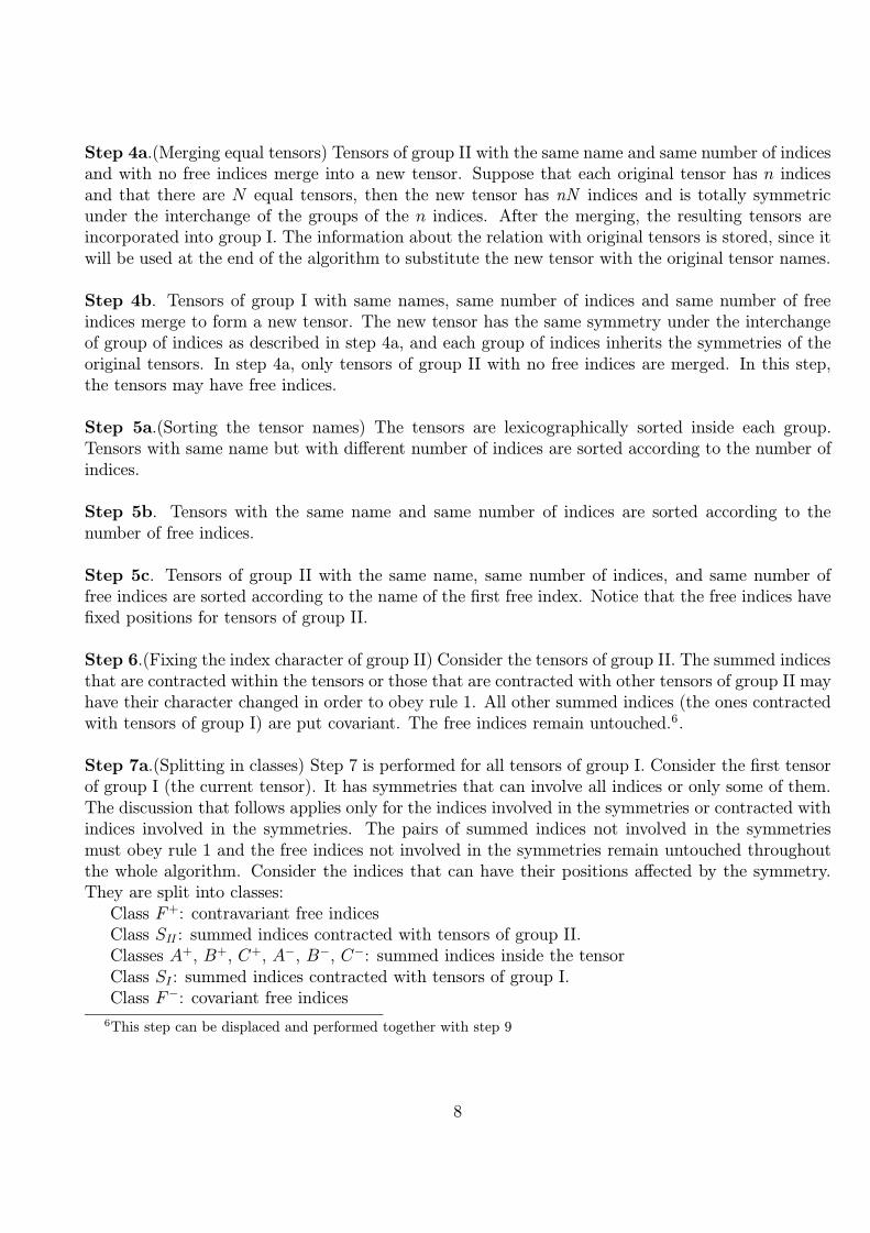
Step 4a.(Merging equal tensors) Tensors of group II with the same name and same number of indicesand with no free indices merge into a new tensor. Suppose that each original tensor has n indicesand that there are N equal tensors, then the new tensor has nN indices and is totally symmetricunder the interchange of the groups of the n indices. After the merging, the resulting tensors areincorporated into group I. The information about the relation with original tensors is stored, since itwill be used at the end of the algorithm to substitute the new tensor with the original tensor names.

Step 4b. Tensors of group I with same names, same number of indices and same number of freeindices merge to form a new tensor. The new tensor has the same symmetry under the interchangeof group of indices as described in step 4a, and each group of indices inherits the symmetries of theoriginal tensors. In step 4a, only tensors of group II with no free indices are merged. In this step,the tensors may have free indices.

Step 5a.(Sorting the tensor names) The tensors are lexicographically sorted inside each group.Tensors with same name but with different number of indices are sorted according to the number ofindices.

Step 5b. Tensors with the same name and same number of indices are sorted according to thenumber of free indices.

Step 5c. Tensors of group II with the same name, same number of indices, and same number offree indices are sorted according to the name of the first free index. Notice that the free indices havefixed positions for tensors of group II.

Step 6.(Fixing the index character of group II) Consider the tensors of group II. The summed indicesthat are contracted within the tensors or those that are contracted with other tensors of group II mayhave their character changed in order to obey rule 1. All other summed indices (the ones contractedwith tensors of group I) are put covariant. The free indices remain untouched.6.

Step 7a.(Splitting in classes) Step 7 is performed for all tensors of group I. Consider the first tensorof group I (the current tensor). It has symmetries that can involve all indices or only some of them.The discussion that follows applies only for the indices involved in the symmetries or contracted withindices involved in the symmetries. The pairs of summed indices not involved in the symmetriesmust obey rule 1 and the free indices not involved in the symmetries remain untouched throughoutthe whole algorithm. Consider the indices that can have their positions affected by the symmetry.They are split into classes:

Class F+: contravariant free indicesClass SII : summed indices contracted with tensors of group II.Classes A+, B+, C+, A−, B−, C−: summed indices inside the tensorClass SI : summed indices contracted with tensors of group I.Class F−: covariant free indices

6This step can be displaced and performed together with step 9

8

Let f+, sII , a, b+, c+, sI , F+, A, B+, C+, SI , C

−, B− and F− respectively. Classes A+ and A− havethe same size.

The summed indices inside the tensor are members of classes A+, B+, C+, A−, B− or C−. Whenboth indices of a pair of summed indices are involved in the symmetries, the contravariant index isa member of class A+, and the covariant is a member of class A−. If a index of a pair of summedindices is involved with the symmetries while the corresponding one is not, there are four cases. Letus call i+ the index involved in the symmetries and i− the corresponding index not involved in thesymmetries. These indices are equal but have different characters (here the signs + and - do notdescribe the character). Suppose that the relative position of i+ with respect to i− cannot be inverteddue to the symmetries. If i+ is at the right of i−, then i+ is a member of class B+; if i+ is at theleft, then i+ is a member of class B−. If the relative positions of i+ and i− can change, then i+ is amember of class C+ or C− depending on whether i+ is contravariant or covariant.

As soon as class A is determined, it is verified whether there are antisymmetric contracted indices.If so, the tensor is null and the algorithm returns to step 2 for the next term.7

The indices of class SI are contracted with the indices of the tensors of group I. Some of the latterindices may not be involved in the symmetries. They form sub-class SI

0, which is further split intoSI

0+

and SI0− , corresponding to the indices of SI

0 contracted with the tensor to the right or to theleft of the current tensor respectively. The remaining indices of SI are split into sub-classes. Theindices of the current tensor contracted with the next (to the right) tensor of group I form the firstsub-class (SI

1); the indices contracted with the next tensor form the second sub-class (SI2), and so

on until the last tensor of group I. If the current tensor is the first of group I, the sub-division inclasses is complete; otherwise the sub-division continues and the next sub-class consists of the indicesthe current tensor contracted with the first tensor of group I. The following sub-class consists of theindices contracted with the second tensor of group I and so on until the last tensor of group I thathas not been considered yet.

Step 7b.(Fixing the index character of group I) In order to obey rule 1, the indices of class SII areput contravariant. The corresponding indices of tensors of group II have already been put covariantin step 6. The indices of class SI are put contravariant if they are contracted with the tensor at theright, or covariant if they are contracted with the tensor at the left of the current tensor. The indicesof class B+ are put contravariant and the corresponding ones are put covariant. The indices of classB− are put covariant and the corresponding ones are put contravariant. The character of the indicesof classes F− is maintained throughout the whole algorithm. The character of classes A+, C+, A−

and C− may still change.

Step 7c.(Ordering and the numbering of the indices) This step establishes the order of the indicesof classes F+, SII , B+, C+, SI , C

−, B− and F− to be used in step 7e. Also, it specifies the numberseach index receives in order for definition 3 to be applied. To begin with, let us discuss the order ofthe indices of classes F+ and F−. First, sort the free indices of class F+ using their original names.The first sorted free index is substituted with the number 1, the second by 2, and so on until the f+

th index, which is substituted with f+. The same process is performed for the indices of class F−,

7The vanishing of the tensor due to the presence of antisymmetric contracted indices can be a natural consequenceof the application of steps 7d to 7f together with lemma 3. For the sake of efficiency, it is better to verify the presenceof antisymmetric contracted indices as soon as class A is determined.

9

which receive the numbers f+ .. a− + 1, · · ·, f+ .. f−.8

Class SII consists of summed indices contracted with the tensors of group II. At this point, thetensors of group II are ordered. The positions of the indices of these tensors are used as a referenceto order the indices of class SII . The first summed index in group II (from left to right) that is amember of class SII is the first index of SII . It receives the number f+ + 1. The second receives thenumber f+ + 2 and so on until f+ + sII .

The indices of classes B+, B−, C+ and C− are contracted with indices that have no symmetries;therefore, they have an ordering reference. They follow the same method used for the indices of classSII .

Class SI can have its sub-classes ordered. The first sub-class is SI0+

, followed by sub-classes SI1,

SI2 and so on, and the last sub-class is SI

0− . The indices of the classes SI0+

and SI0− can be ordered

since they are contracted with indices not involved in the symmetries. They follow the same methodused for the indices of class SII . The indices of the other sub-classes cannot be ordered at this point.Also, the indices of class A cannot be ordered at this point.

Here follows, explicitly, the numbers reserved for each class:Class F+: 1, 2, · · ·, f+

Class SII : f+ + 1, f+ + 2, · · ·, f+ + sII

Class A+: f+ + sII + 1, · · ·, f+ .. a+

Class B+: f+ .. a+ + 1, · · ·, f+ .. b+

Class C+: f+ .. b+ + 1, · · ·, f+ .. c+

Class SI : f+ .. c+ + 1, · · ·, f+ .. sI

Class C−: f+ .. sI + 1, · · ·, f+ .. c−

Class B−: f+ .. c− + 1, · · ·, f+ .. b−

Class A−: f+ .. b− + 1, · · ·, f+ .. a−

Class F−: f+ .. a− + 1, · · ·, f+ .. f−

Step 7d.(Generating the character configurations) Both indices of a pair from class A can changetheir positions due to the symmetries, but the relative position of some pairs may be fixed. Thecharacters of the pairs, that cannot invert the relative position, can be chosen such that they obeyrule 1. The characters of the remainder indices of class A (let a0 be the number of pairs of classA that can invert their relative position) and the characters of indices of class C cannot be chosena priori. Each pair has two states which are contravariant-covariant and covariant-contravariant,corresponding to the characters of the indices. The algorithm generates 2(a0+c) possible characterconfigurations by changing the states of pairs that can invert their relative position.

If the current tensor is totally symmetric, steps 7d and 7f need not be performed. The canonicalform can be obtained straightforwardly, avoiding the slowest steps.

Step 7e.(Applying the symmetries) At this point, more than one equivalent configuration may havebeen generated. The symmetries are applied to all configurations in order to perform the followingtasks.9 The contravariant indices are pushed to the left positions as far as possible and the covariant

8The notation f+ .. f− means f+ + sII + a+ + b+ + c+ + sI + c− + b− + a− + f−. The variables a+ and a− areequal to a.

9The application of the symmetries is a straightforward procedure that can be implemented for each kind ofsymmetry. In the case of the Maple system, tensors can be represented by tables and the symmetries by indexingfunctions, which can perform the tasks described in step 7e.

10

indices to right positions as far as possible. A sign change may be generated if there are antisymmetricindices. The state configurations that are members of the set of character normal configurations ofthe current tensor are selected. The symmetries are applied to the selected configurations again inorder to put classes F+, SII , A+, B+, C+, SI , C

−, B−, A− and F− as closely as possible in thesmallest position as prescribed in definition 3a, and after that, the indices of classes F+, SII , B+,C+, SI

0, C−, B−, and F− are put as closely as possible in their order as prescribed in definition 3b(see step 7c for relabelling). The sub-set of index normal configurations is selected. At this point,the character and the positions of all classes have been determined. Only the order of the indices ofclass A and of the indices of the sub-classes of SI (not including SI

0) has not been determined yet.

Step 7f.(Generating equivalent configurations of class A) In general, the ordering of the indices ofthe sub-classes of SI depends on the ordering of the indices of class A and vice-versa. These classesmust be ordered together. For now, suppose that all classes SI

i (i > 0) are empty. In this case, steps7a to 7g can be performed for each factor of the product since they are independent of each other.

The aim of this step is the generation of permutations of class A that preserve the characterarrangement of the indices. The selected configurations of step 7e are submitted to all possiblere-orderings of class A (class A+ plus A−) allowed by induced symmetry of the indices of class A+

together with the indices of class A−. The character normal configurations are selected.If the induced symmetry of class A is totally symmetric, the generation of permutation are not

necessary since the canonical positions can be obtained straightforwardly.In many cases, it is sufficient to generate the re-orderings allowed by the induced symmetries of

class A+ and class A− independently. This kind of re-ordering automatically maintain the characterconfiguration.

Step 7g.(Selecting the index canonical configuration) The indices of all configurations are substitutedby their correspondent numbers (step 7c), and the index canonical configuration with respect toclasses F+, SII , A+, B+, C+, SI , C

−, B−, A− and F− is selected.If two elements with the index canonical configuration are selected and they have opposite signs

then the current product is zero (lemma 3). In this case, the algorithm returns to step 2 for the nextterm.

Step 7h.(Ordering indices of the sub-classes of SI) The order of the sub-classes of SI and the orderof the indices of SI

0 have already been determined. The present step finds out the order of theindices of sub-classes SI

i (i > 0) of all tensors of the current product. Consider class A and all sub-classes SI

i (i > 0) of the first tensor. These classes together have a induced symmetry. The samecan be stated about the other factors of the product. All indices of all classes A and all sub-classesSI

i (i > 0) of all factors are put together in order to form a new tensor totally contracted. Theorder of the indices in the new tensor follows the order of the factors and the order of appearance ineach factor. The symmetries of the new tensor is composed by all induced symmetries acting in thecorresponding indices (see example 2).

By a recursive call of the algorithm, the indices of the new tensor are in class A and are orderedby the method described for this class. The dummy indices that come from sub-classes SI

i cannotinvert their relative positions (within a pair) hence step 7d need not generate character configurationsfor these indices.

If the induced symmetry of the indices of the sub-classes SIi of a factor coincides with the actual

11

symmetry of these indices (taking into account the contractions of class A) then the indices of classA of this factor need not be included in the new tensor.

Step 8.(Recovering merged tensors) The symmetric (by group of indices) tensors that have beenformed by merging tensors with equal names, equal number of indices and equal number of freeindices in step 4a and 4b are converted back by the inverse process to a product of tensors with theoriginal names but with the new positions of indices generated by the previous steps.

Step 9.(Renaming the dummy indices) At this stage of the algorithm, the indices are in their finalposition. The dummy indices are renamed following the rules: There are two cases. The first occurswhen the whole pair of dummy indices resides inside a tensor. If the tensor name is A and thenumber of indices is m, then the dummy index name will be A m i j , where i is the position of thecontravariant index and j is the position of the covariant index and is some separator.10 If thesame name appears in other tensors of the product, no name conflict is generated. The second caseoccurs when the dummy indices involve two tensors. Suppose that the first tensor has the nameA with m indices and the second has the name B with n indices, then the dummy index will berenamed A m i B n j , where i is the position of the contravariant index inside the tensor A andj is the position of the covariant index inside the tensor B. This renaming process proceeds fromleft to right. If a second dummy index receives the same name, then the number 1 is appended inits name A m i B n j 1 , for example. If a third summed index receives the same name, then thenumber 2 is appended in its name: A m i B n j 2 , and so on.11

Step 10.(Collecting equal tensor terms) After performing steps 1 to 9 for all terms, collect equaltensor products and put the coefficient factors into the canonical form.

Step 11.(Sorting the addition)12 Each tensor product can be converted to a string by concatenatingwith separators the names of the tensors and the indices in the order they appear in the product.These strings are sorted. The order of the terms in the sum is rearranged to be in the same order asthe sorted concatenated strings.

2.3 Proof that the algorithm is a canonical function

Let T be the set of all tensor expressions which obey hypothesis 1. The algorithm described insection 2.2 is a function F : T 7−→ T .

Theorem: F is a canonical function.Demonstration: The proof has three parts.

1. All operations performed by the algorithm obey the rules of the tensor algebra, hence preservethe mathematical equivalence of tensor expressions.

10The separator is a symbol not present in tensor expressions.11The method of appending a number to the repeated dummy index names can be fully avoided if step 8 is performed

after step 9.12In general, this step is not necessary when the algorithm is implemented over multiple purpose computer algebra

systems.

12

2. For all E 1, E 2 ∈ T such that E 1 = E 2, F(E 1) ≡ F(E 2). After step 1, E 1 and E 2 are sumsof tensor products. Consider a generic tensor product. It is clear from the sorting uniqueness thatthe position of the tensors is unique after the application of the algorithm. The indices of tensors ofgroup II and the indices of classes F+, SII , B+, SI , B

− and F− of tensors of group I go to a uniquecharacter configuration, since this is a matter of convention.

The proof that the indices of tensors of group I (including the merged tensors of step 4) cometo a unique configuration is consequence of the fact that the algorithm runs over all index characterconfigurations of the indices of classes A and C and over all allowed index position configurationsof classes A and SI . Only one configuration is selected as the canonical configuration unless theproduct is zero (lemma 3). After step 9, the dummy indices have canonical names, completing thecanonicalization of a tensor product. Steps 10 and 11 put a sum of tensor products into the canonicalform.

3. In item 2 is missing the details about the special case when one tensor expression is zero,that is, if E = 0 then F(E) ≡ 0. From lemmas 1 and 2 follow that the indices responsible for thecancelation of a factor are in class A and for a product are in class SI . Since the algorithm generatesthe set of all mathematically equivalent tensor products by permuting the indices of classes A andSI , lemma 3 garantee that any null product inside the tensor expression is recognized. Other non-null tensor products that may still exist are put into a canonical form (item 2) guaranteeing thecancellation of a sum of products in step 10.

In the algorithm, there are shortcuts for special kinds of symmetries avoiding the generation ofcharacter configurations of step 7d or permutations of step 7f. These shortcuts increase the efficiencybut they must satisfy items 1-3 of the proof.

2.4 Examples

Example 1: Consider the tensor expression R ib a i (contraction of the Riemann tensor). Step 7a

establishes that classes A and F − are the only non empty classes in this case. Class A+ is [i+] ,class A− is [i−] and class F − is [a, b]. Step 7c establishes that the contravariant index i receivesthe number 1, the covariant index i receives the number 2, and the indices a and b receive thenumbers 3 and 4 in this order, since a precedes b. Step 7d establishes that there are two characterconfigurations to be considered: R i

b a i and R i b ai. The symmetries are applied (step 7e) in order

to put these configurations into the equivalent ones R ib i a and R i

a i b. Both are selected, since bothare members of the set of character normal configurations. No further changes are generated by thesymmetries, so the configurations that are members of the set of index normal configurations mustbe selected. The indices are substituted with their respective numbers, yielding [1,4,2,3] and [1,3,2,4]respectively. Definition 3a with respect to the partition (1,1,2) – corresponding to classes [1], [2] and[3,4] – selects both configurations. Definition 3b with respect to class [3,4] selects [1,3,2,4] as theonly member of the set of index normal configurations. Since there are no induced symmetries, nomore index configurations are generated. The index canonical configuration is [1,3,2,4] . Therefore,the canonical form is R i

a i b, where i is R 4 1 3 , as prescribed in step 9.

Example 2: Consider the tensor expression T j S k l T iR i l j k, where S k l is a totally symmetrictensor and R i l j k is the Riemann tensor. Step 3 splits the expression into group I: [S k l, R i l j k]

13

and group II: [T j , T i]. Step 4b merges T j and T i into one totally symmetric tensor (let be calledT T j i) and adds to group I. Group II is empty now. Step 5a establishes the order for group I:[R i l j k, S

k l, T T j i]. Step 7a establishes that the only non-empty class in this case is SI . For thefirst tensor one has SI

1 = [l, k] and SI2 = [j, i]. The order of these indices has not been established

yet. These are the only classes since all indices have been covered. Step 7b fixes the character as:[R i l j k, S k l, T T j i]. Step 7e converts R i l j k into R l i k j and maintains S k l and T T j i invariant.Step 7h generates a new tensor. Let us call N l i k j

k l j i. It has the symmetries of the Riemanntensor (excluding the cyclic symmetry) in the first four indices (l +,i +,k +,j +); is symmetric underthe interchange of the fifth and sixth indices (k −,l −) and is symmetric under the interchange of theseventh and eighth indices (j −,i −). The algorithm is called recursively, and N l i k j

k l j i is convertedto N l i k j

l k i j , determining the order of the indices. After step 8 one has: [R l i k j , S l k, T i, T j ].Step 9 establishes that canonical form for the expression is R l i k j S l k T i T j where l = R 4 1 S 2 1 ,i = R 4 2 T 1 1 , k = R 4 3 S 2 2 and j = R 4 4 T 1 1 .

3 An experimental implementation

Algorithms to simplify tensor expressions have been implemented in some computer algebra sys-tems.[15][16][17][18][19] Some implementations use pattern matching which requires a big databaseof tensor rules, and even worse, sometimes the user must enter the rules. The underlying methodused by the Ricci package[15] seems similar in some aspects to the method presented here. All theseimplementations have not solved the dummy index problem, therefore the main simplifier spends along time or cannot simplify tensor expressions with many dummy indices.

In this section, I present an experimental implementation of the algorithm described in section 2over the Riemann package.[7] The new package can be obtained from web sites,13 and my purpose isto supersede the Riemann package in the near future with the new functionalities introduced to dealwith tensor components abstractly.

The function normalform uses the algorithm to put tensor expressions into normal forms. Noattempt has been made to put the output into the canonical form, that is, ordered with respect tothe sum and to the product of terms, since this last step is unnecessary for the purpose of any generalcomputer algebra system.

In the examples below, contravariant indices have positive signs and covariant indices have neg-ative signs. Tensors are indexed variables and their symmetries are declared by the command de-finetensor. Some tensors are pre-defined: Christoffel symbols, Riemann tensor, Ricci tensor andRicci scalar are pre-defined with the names Γ (Christoffel symbols) and R (Riemann, Ricci and Ricciscalar). More details can be found in the new help pages for the commands normalform, definetensorand symmetrize, and in the help pages of the Riemann package.

Expressions that are zero due to tensor symmetries are readily simplified:14

> readlib(showtime)():> definetensor(T[i,j,k,l], sym[1,2] and asym[3,4]);

13See the addresses: http://www.cbpf.br/˜portugal/Riegeom.html or http://www.astro.queensu.ca/˜portugal/Rie-geom.html

14All calculations have been performed in a Pentium 120 MHz with 32 Mb of RAM, running Maple V release 5 overWindows 95.

14

T i j k l

time = 0.01, bytes = 13478> expr1 := printtensor(R[i,j,k,l]*T[-i,-k,-j,-l]);

R i j k l T i k j l

time = 0.05, bytes = 8124> normalform(expr1);

0

time = 0.12, bytes = 90619> expr2 := printtensor(T[i,j,k,l]*V[-i]*V[-j]+V[b]*V[a]*T[-a,-b,l,k]);

T i j k l V i V j + V b V a T a bl k

time = 0.01, bytes = 8042> normalform(expr2);

0

time = 0.30, bytes = 338050> off;Polynomials constructed with the Riemann tensor exemplify the algorithm’s worst performance.

No special techniques have been implemented for the kind of symmetries of the Riemann tensor.In the next example, all possible ways to write the scalars formed by the product of two Riemanntensors are generated. The 40.320 expressions reduce to 4 independent non-null forms if the cyclicidentity of the Riemann tensor is not considered. In the next section, one can verify that the cyclicidentity reduces to 3 independent scalars (cf. ref. [1]).15

> S := {op(combinat[permute]([a,b,c,d,-a,-b,-c,-d]))}:> nops(S);

40320

> readlib(showtime)():> S1 := map(x->abs(normalform(R[op(1..4,x)]*R[op(5..8,x)])), S);

{0,∣∣∣R R1R1 R2R2 R3R3 R4R4 R R1R1 R2R2 R3R3 R4R4

∣∣∣ , ∣∣∣R R1R1 R2R3 R3R2 R4R4 R R1R1 R3R2 R2R3 R4R4

∣∣∣ ,∣∣∣R R1R1 R2R2 RR1R1 R2R2

∣∣∣ , |(R)|2}

15Simplified names for the dummy indices are used for this demonstration. This choice does not provide trulycanonical names.

15

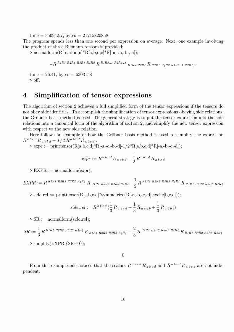
time = 35094.97, bytes = 21215820858The program spends less than one second per expression on average. Next, one example involvingthe product of three Riemann tensors is provided:

> normalform(R[-c,-d,m,n]*R[a,b,d,c]*R[-n,-m,-b ,-a]);

−R R1R3 R2R4 R3R1 R4R2 R R1R3 1 R2R4 1R1R3 R2R4 R R3R1 R4R2 R1R3 1 R2R4 1

time = 26.41, bytes = 6303158> off;

4 Simplification of tensor expressions

The algorithm of section 2 achieves a full simplified form of the tensor expressions if the tensors donot obey side identities. To accomplish the simplification of tensor expressions obeying side relations,the Grobner basis method is used. The general strategy is to put the tensor expression and the siderelations into a canonical form of the algorithm of section 2, and simplify the new tensor expressionwith respect to the new side relation.

Here follows an example of how the Grobner basis method is used to simplify the expressionR a b c dR a c b d − 1/2 R a b c dR a b c d .

> expr := printtensor(R[a,b,c,d]*R[-a,-c,-b,-d]-1/2*R[a,b,c,d]*R[-a,-b,-c,-d]);

expr := R a b c dR a c b d −1

2R a b c dR a b c d

> EXPR := normalform(expr);

EXPR := R R1R1 R2R3 R3R2 R4R4 R R1R1 R3R2 R2R3 R4R4−1

2R R1R1 R2R2 R3R3 R4R4 R R1R1 R2R2 R3R3 R4R4

> side rel := printtensor(R[a,b,c,d]*symmetrize(R[-a,-b,-c,-d],cyclic[b,c,d]));

side rel := R a b c d (1

3R a b c d +

1

3R a c d b +

1

3R a d b c)

> SR := normalform(side rel);

SR :=1

3R R1R1 R2R2 R3R3 R4R4 R R1R1 R2R2 R3R3 R4R4 −

2

3R R1R1 R2R3 R3R2 R4R4 R R1R1 R3R2 R2R3 R4R4

> simplify(EXPR,{SR=0});

0

From this example one notices that the scalars R a b c dR a c b d and R a b c dR a b c d are not inde-pendent.

16

5 Conclusion

An algorithm to simplify tensor expressions based on computable definitions have been described.It has two parts. In the first part, the expression is put into a canonical form, taking into accountsymmetries with respect to index permutations and the renaming of dummy indices. The definitionof the canonical form involves some conventions that can be changed without disqualifying thedefinition. The conventions are based on the implementation simplicity and on a readable displayfor tensor expression. In the second part, cyclic identities or more general kinds of tensor identitiesare addressed through the Grobner basis method. The expression and the side relations are bothput into a canonical form for the Grobner method to work successfully.

In this work, a precise definition of the canonical form for tensor expressions is provided. Norestriction is imposed on the kind of symmetries that the tensors can obey. For most of the symmetriesthat occur in practise, the algorithm is very fast. The symmetries of the Riemann tensor reveal thealgorithm’s worst performance, but even in in this case it is useful for practical applications.

The invariant renaming of the dummy indices plays an important role in the efficiency of thealgorithm, since it neutralizes the symmetries that come from dummy index renaming. This is asolution for the dummy indices problem mentioned in the introduction.

An experimental implementation of the algorithm over the Riemann package[7] is available freefrom web sites.16 All calculations and timings presented in this work can be reproduced in the Maplesystem.

Acknowledgements:I thank Ray McLenaghan and Keith Geddes for pointing out references and for the kind hospitality

at the University of Waterloo. This work was made possible by a fellowship from CAPES, Ministerioda Educacao e do Desporto, Brazil.

References

[1] S. A. Fulling, R. C. King, B. G. Wybourne and C. J. Cummins, Normal forms for tensorpolynomials: I. The Riemann tensor, Class. Quantum Grav. 9 (1992) 1151-1197.

[2] V. A. Ilyin and A. P. Kryukov, ATENSOR - REDUCE program for tensor simplification, Com-puter Physics Communications 96 (1996) 36-52.

[3] A. Dresse, PhD thesis, Universite Libre de Bruxelles, 1993.

[4] B. G. Wybourne and J. Meller, Enumeration of the order-14 invariants formed from the Riemanntensor, J. Phys. A25 (1992) 5999-6003.

[5] G. Butler and C. W. H. Lam, A general backtrack algorithm for the isomorphism problem ofcombinatorial objects, J. Symb. Comput. 1 (1985) 363-381.

16See footnote 12.

17

[6] K. O. Geddes, S. R. Czapor and G. Labahn, Algorithms for Computer Algebra, Kluwer AcademicPublisher, 1992.

[7] Portugal, R. and Sautu , S., Applications of Maple to General Relativity, Computer PhysicsCommunications 105 (1997) 233-253.

[8] Waterloo Maple, Inc., 450 Phillip Street, Waterloo, Ontario, N2L 5J2, Canada. See the webpages: http://www.maplesoft.com/

[9] D. Lovelock and H. Rund, Tensors, Differential Forms and Variational Principles, John Wiley& Sons, 1975.

[10] L. P. Eisenhart, Riemannian Geometry, Princeton University Press, 1966.

[11] T. Y. Thomas, Tensor Analysis and Differential Geometry, Academic Press, 1965.

[12] D. E. Littlewood, The Theory of Group Characters and Matrix Representations of Groups,Oxford University Press, 1950.

[13] B. L. van der Waerden, Algebra, Frederick Ungar Publishing Co., 1970.

[14] N. Pelavas and R. Portugal, to appear.

[15] J. M. Lee, D. Lear and J. Roth, Ricci - A Mathematica package for doing tensor cal-culations in differential geometry (User’s Manual version 1.2) 1995. See the web pageshttp://www.math.washington.edu/˜lee/Ricci.

[16] L. Parker and S. M. Christensen, MathTensor, A System for Doing Tensor Analysis by Com-puter, Addison-Wesley, 1994.

[17] R. Bogen et al., Macsyma Reference Manual, vol II, chapter V2-3, Laboratory for ComputerScience, MIT, 1983.

[18] L. Hornfeldt, STENSOR user guide and STENSOR reference manual, University of Stockholm,Institute of Theoretical Physics, 1988. (See also M. A. H. MacCallum and J. Skea, Sheep: Acomputer algebra system for General Relativity, Lecture Notes from the First Brazilian Schoolon Computer Algebra, vol. 2, eds. M. J. Reboucas and W. L. Roque, Claredon Press, Oxford,1994.)

[19] M. Kavian, R. G. McLenaghan and K. O. Geddes, MapleTensor: Progress Report on a NewSystem for Performing Indicial and Component Tensor Calculation using Symbolic Computa-tion, ISSAC’96, Proceedings of the 1996 International Symposium on Symbolic and AlgebraicComputation (ETH 1996), Y. N. Lakshman, Ed., pp.204.

18