An Algebraic Approach to Symmetrywith Applications to Knot Theory

by

David Edward Joyce

A dissertation in mathematics

Presented to the Graduate Faculty of the University of Pennsylvania in partial fulfillment ofthe requirements for the degree of Doctor of Philosophy

1979

[signed]Peter J. FreydSupervisor of Dissertation

[signed] Jerry L. KazdanGraduate Group Chairman

1

Preface

This edition of my dissertation differs little from the original 1979 version. This edition istypeset in LATEX, whereas the original was typed on a typewriter and the figures were handdrawn. The page numbers and figure numbers are changed, the table of contents is expandedto include sections, a list of figures is included, and the index appears at the end instead ofthe front. I’ve corrected a few typos (and probably added others), and I added figure 4.5that was missing from the original.

David JoyceJune, 2009

i

Acknowledgments

I thank my friends for their tolerance, nay, for their encouragement, of the investigationof the mathematics herein presented. I owe much to Julian Cole for many encouragingdiscussions and for some suggestions concerning nomenclature. I owe much more to myadviser, Peter Freyd, for his continued guidance of my mathematical maturity and for manydiscussions in many fields, mathematical and otherwise. I give special thanks to Janet Burnsfor the fine job of typing this dissertation.

Abstract

The usual algebraic construction used to study the symmetries of an object is the groupof automorphisms of that object. In many geometric settings, however, one may interpret thesymmetries in a more intimate manner by an algebraic structure on the object itself. Define aquandle to be a set equipped with two binary operations, (x, y) 7→ x . y and (x, y) 7→ x .-1 y,which satisfies the axioms

Q1. x . x = x.Q2. (x . y) .-1 y = x = (x .-1 y) . y.Q3. (x . y) . z = (x . z) .(y . z).

Call the map S(y) sending x to x . y the symmetry at y.To each point y of a symmetric space there is a symmetry S(y) of the space. By defining

x . y = x .-1 y to be the image of x under S(y), the symmetric space becomes a quandle. Calla quandle satisfying x . y = x .-1 y an involutory quandle. Loos [7] has defined a symmetricspace as a manifold with an involutory quandle structure such that each point y is an isolatedfixed point of S(y).

The underlying set of a group G along with the operations of conjugation, x . y = y−1xyand x .-1 y = yxy−1 form a quandle ConjG. Moreover, the theory of conjugation may beregarded as the theory of quandles in the sense that any equation in . and .-1 holding inConjG for all groups G also holds in any quandle. If the center of G is trivial, then ConjGdetermines G.

Let G be a group and n ≥ 2. The n-core of G is the set

(x1, x2, . . . , xn) ∈ Gn |x1x2 . . . xn = 1

along with the operation

(x1, x2, . . . , xn) .(y1, y2, . . . , yn) = (y−1n xny1, y−11 x1y2, . . . , y

−1n−1xn−1yn).

The n-core is an n-quandle, that is, each symmetry has order dividing n. The group G issimple if and only if its n-core is a simple quandle.

Let G be a noncyclic simple group and Q a nontrivial conjugacy class in H viewed as asubquandle of ConjG. Then Q is a simple quandle.

Let Q be a quandle. The transvection group of Q, TransQ, is the automorphism group ofQ generated by automorphisms of the form S(x)S(y)−1 for x, y in Q. Suppose Q is a simplep-quandle where p is prime. Then either TransQ is a simple group, or else Q is the p-core ofa simple group G and TransQ = Gp.

ii

Consider the category of pairs of topological spaces (X,K), K ⊆ X, where a map f :(X,K) → (Y, L) is a continuous map f : X → Y such that f−1(L) = K. Let (D,O) bethe closed unit disk paired with the origin O. Call a map from (D,O) to (X,K) a noose inX about K. The homotopy classes of nooses in X about K form the fundamental quandleQ(X,K). The inclusion of the unit circle to the boundary of D gives a natural transformationfrom Q(X,K) to the fundamental group π1(X−K). A statement analogous to the Seifert-VanKampen theorem for the fundamental group holds for the fundamental quandle.

Let K be an oriented knot in the 3-sphere X. Define the knot quandle Q(K) to be thesubquandle of Q(X,K) consisting of nooses linking once with K. Then Q(K) is a classifyinginvariant of tame knots, that is, if Q(K) = Q(K ′), then K is equivalent to K ′. The knotgroup and the Alexander invariant can be computed from Q(K).

[8] Loos, O., Symmetric Spaces, Benjamin, New York, 1969.

iii

Contents

List of Figures v

1 Definitions and Examples 11.1 Quandles . . . . . . . . . . . . . . . . . . . . . . . . . . . . . . . . . . . . . . . 11.2 Involutory quandles . . . . . . . . . . . . . . . . . . . . . . . . . . . . . . . . . 3

2 Representations and the general algebraic theory of quandles 52.1 The algebraic theory of conjugation . . . . . . . . . . . . . . . . . . . . . . . . 52.2 Automorphism groups of quandles . . . . . . . . . . . . . . . . . . . . . . . . . 62.3 Representation of quandles as conjugacy classes . . . . . . . . . . . . . . . . . 62.4 Representation of quandles as cosets . . . . . . . . . . . . . . . . . . . . . . . 72.5 Algebraic connectivity . . . . . . . . . . . . . . . . . . . . . . . . . . . . . . . 82.6 The transvection group . . . . . . . . . . . . . . . . . . . . . . . . . . . . . . . 92.7 n-Cores . . . . . . . . . . . . . . . . . . . . . . . . . . . . . . . . . . . . . . . 92.8 Examples of simple quandles . . . . . . . . . . . . . . . . . . . . . . . . . . . . 102.9 Classification of simple p-quandles . . . . . . . . . . . . . . . . . . . . . . . . . 122.10 Augmented quandles . . . . . . . . . . . . . . . . . . . . . . . . . . . . . . . . 142.11 Quotients of augmented quandles described by normal subgroups of the aug-

mentation group . . . . . . . . . . . . . . . . . . . . . . . . . . . . . . . . . . 18

3 Involutory quandles 213.1 Involutory quandles and geodesics . . . . . . . . . . . . . . . . . . . . . . . . . 213.2 Involutory quandles generated by two points . . . . . . . . . . . . . . . . . . . 223.3 Group cores . . . . . . . . . . . . . . . . . . . . . . . . . . . . . . . . . . . . . 233.4 Distributive quandles . . . . . . . . . . . . . . . . . . . . . . . . . . . . . . . . 253.5 Involutions . . . . . . . . . . . . . . . . . . . . . . . . . . . . . . . . . . . . . . 283.6 Moufang loop cores . . . . . . . . . . . . . . . . . . . . . . . . . . . . . . . . . 283.7 Distributive 2-quandles with midpoints . . . . . . . . . . . . . . . . . . . . . . 31

4 Algebraic topology and knots 334.1 The fundamental quandle of a pair of spaces. . . . . . . . . . . . . . . . . . . . 334.2 The fundamental quandle of a disk . . . . . . . . . . . . . . . . . . . . . . . . 374.3 The Seifert-Van Kampen theorem . . . . . . . . . . . . . . . . . . . . . . . . . 384.4 Applications of the Seifert-Van Kampen theorem . . . . . . . . . . . . . . . . 404.5 Knot quandles . . . . . . . . . . . . . . . . . . . . . . . . . . . . . . . . . . . . 414.6 A presentation of the knot quandle . . . . . . . . . . . . . . . . . . . . . . . . 42

iv

4.7 The invariance of the knot quandle . . . . . . . . . . . . . . . . . . . . . . . . 444.8 A presentation of the knot quandle (continued) . . . . . . . . . . . . . . . . . 454.9 A representation of the knot quandle . . . . . . . . . . . . . . . . . . . . . . . 474.10 The Alexander invariant of a knot . . . . . . . . . . . . . . . . . . . . . . . . . 484.11 The cyclic invariants of a knot . . . . . . . . . . . . . . . . . . . . . . . . . . . 504.12 The involutory knot quandle . . . . . . . . . . . . . . . . . . . . . . . . . . . . 50

Bibliography 53

Index 55

v

List of Figures

1.1 The trefoil knot . . . . . . . . . . . . . . . . . . . . . . . . . . . . . . . . . . . 4

2.1 A singular 2-quandle . . . . . . . . . . . . . . . . . . . . . . . . . . . . . . . . 7

3.1 QG3 . . . . . . . . . . . . . . . . . . . . . . . . . . . . . . . . . . . . . . . . . 213.2 Geodesics . . . . . . . . . . . . . . . . . . . . . . . . . . . . . . . . . . . . . . 223.3 Singular quandles Cs(4) and CS(8) . . . . . . . . . . . . . . . . . . . . . . . . 233.4 Distributivity . . . . . . . . . . . . . . . . . . . . . . . . . . . . . . . . . . . . 253.5 Midpoints . . . . . . . . . . . . . . . . . . . . . . . . . . . . . . . . . . . . . . 32

4.1 The noose N . . . . . . . . . . . . . . . . . . . . . . . . . . . . . . . . . . . . 344.2 A noose homotopy . . . . . . . . . . . . . . . . . . . . . . . . . . . . . . . . . 354.3 q and q−1 . . . . . . . . . . . . . . . . . . . . . . . . . . . . . . . . . . . . . . 364.4 Seifert-Van Kampen noose homotopy . . . . . . . . . . . . . . . . . . . . . . . 394.5 Noose boundary loops . . . . . . . . . . . . . . . . . . . . . . . . . . . . . . . 424.6 The figure-8 knot . . . . . . . . . . . . . . . . . . . . . . . . . . . . . . . . . . 424.7 A knot crossing . . . . . . . . . . . . . . . . . . . . . . . . . . . . . . . . . . . 434.8 Basic knot deformations . . . . . . . . . . . . . . . . . . . . . . . . . . . . . . 444.9 Invariance under Ω1 . . . . . . . . . . . . . . . . . . . . . . . . . . . . . . . . . 444.10 Invariance under Ω2 . . . . . . . . . . . . . . . . . . . . . . . . . . . . . . . . . 454.11 Invariance under Ω3 . . . . . . . . . . . . . . . . . . . . . . . . . . . . . . . . . 454.12 The loop γi . . . . . . . . . . . . . . . . . . . . . . . . . . . . . . . . . . . . . 464.13 The trefoil knot 31 . . . . . . . . . . . . . . . . . . . . . . . . . . . . . . . . . 514.14 The figure-8 knot 41 . . . . . . . . . . . . . . . . . . . . . . . . . . . . . . . . 514.15 The knot 10124 . . . . . . . . . . . . . . . . . . . . . . . . . . . . . . . . . . . 514.16 Q2(10124) . . . . . . . . . . . . . . . . . . . . . . . . . . . . . . . . . . . . . . 524.17 Two links with homeomorphic complements but different quandles . . . . . . . 53

vi

Chapter 1

Definitions and Examples

1.1 Quandles

Let Q be a set equipped with a binary operation, and denote this operation by (x, y) 7→ x . y.We use the nonsymmetric symbol . here since the two variables will play different roles inthe following discussion. Also, it will distinguish this binary operation from others that Qmay have, in particular, addition and multiplication.

For z in Q, let S(z) be the function on Q whose value at x is x . z. It will be moreconvenient for us to use the notation xS(z) = x . z rather than S(z)(x) = x . z. For S(z) tobe a homomorphism, we require

(x . y)S(z) = xS(z) . yS(z),

that is,

(1) (x . y) . z = (x . z) .(y . z).

When (1) holds for all x, y, z in Q, S is a function from Q to EndQ, the set of endomorphismsof Q. If S(z) is also a bijection for all z, then S maps Q to AutQ, the group of automorphismsof Q. Any group, in particular AutQ, has the operation of conjugation, f . g = g−1fg,which satisfies (1). Then S : Q → AutQ is itself a homomorphism. That is S(y . z) =S(z)−1S(y)S(z), equivalently, S(z)S(y . z) = S(y)S(z), which is a restatement of (1). Therequirement that S(z) be a bijection for all z is equivalent to the existence of another binaryoperation

(x, y) 7→ x .-1 y

that satisfies

(2) x . y = z ⇐⇒ x = z .-1 y.

An equational identity equivalent to (2) is

(3) (x . y) .-1 y = x = (x .-1 y) . y.

From (1) and (2) we may derive the identities

(x . y) .-1 z = (x .-1 z) .(y .-1 z),

(x .-1 y) . z = (x . z) .-1(y . z),

(x .-1 y) .-1 z = (x .-1 z) .-1(y .-1 z).

1

In all the applications that follow, S(z) will not only be an automorphism, but one whichfixes z.

Definition. A quandle is a set Q equipped with two binary operations (x, y) 7→ x . y and(x, y) 7→ x .-1 y which satisfies three axioms

Q1. x . x = x.

Q2. (x . y) .-1 y = x = (x .-1 y) . y.

Q3. (x . y) . z = (x . z) .(y . z).

The map S(z) is called the symmetry at z, and x . z may be read as “x through z”. Theaxioms taken together say that the symmetry at any point of Q is an automorphism of Qfixing that point. The order of a quandle is the cardinality of its underlying set. The elementsof a quandle will be frequently referred to as points.

Example 1. A group G is a quandle, denoted ConjG, with conjugation as the operation.x . y = y−1xy, x .-1 y = yxy−1. Any conjugacy class of G is a subquandle of ConjG as is anysubset closed under conjugation. When G is Abelian, the operation becomes simply the firstprojection operation, x . y = x.

Definition. A quandle Q is said to be Abelian if it satisfies

QAb. (w .x) .(y . z) = (w . y) .(x . z).

It follows from the definition that an Abelian quandle also satisfies the identities

(w .-1 x) .(y .-1 z) = (w . y) .-1(x . z)

(w .-1 x) .-1(y .-1 z) = (w .-1 y) .-1(x .-1 z)

Example 2. Let T be a nonsingular linear transformation on a vector space V . Then Vbecomes a quandle with the operations x . y = T (x − y) + y and x .-1 y = T−1(x − y) + y.Moreover, V is an Abelian quandle.

It should be noted that quandles are seldom associative. In fact, the identity (x . y) . z =x .(y . z) is equivalent to the identity x . y = x. One associativity equation which does holdfor any quandle is (x . y) . x = x .(y . x). To reduce the number of parentheses we use thenotation x . y . z for (x . y) . z.

By far the most interesting axiom for quandles is the distributivity axiom Q3. The firststudy of self-distributivity is that of Burstin and Mayer [5]. They define “distributive groups”,or in modern terminology, distributive quasigroups. A quasigroup is a set G equipped witha binary operation (x, y) 7→ xy such that for all a, b in G there exist unique solutions x, y tothe equations xa = b and ay = b. A quasigroup is distributive if it satisfies the two identities

(xy)z = (xz)(yz), and

x(yz) = (xy)(xz).

It follows that a distributive quasigroup is idempotent, xx = x. Hence, quandles are ageneralization of distributive quasigroups. Burstin and Mayer define an “Abelian distributivegroup” to be one satisfying

(wx)(yz) = (wy)(xz).

This axiom goes by the names “entropy”, “mediality”, “surcommutativity”, and “symmetry”.

2

1.2 Involutory quandles

An important class of quandles are those in which the symmetries S(z) are all involutions,S(z)2 is the identity. In this case x . z = x .-1 z, which allows us to dispense with the secondquandle operation. An equivalent condition is the identity

QInv. x . y . y = x.

Definition. A quandle satisfying QInv is called an involutory quandle or 2-quandle. Al-ternatively, an involutory quandle may be defined as a set equipped with a binary operation(x, y) 7→ x . y which satisfies Q1, Qinv, and Q3. Analogously an n-quandle is a quandlesuch that for all x, y, xS(y)n = x. In any quandle let x .n y denote xS(y)n.

Example 1. Let G be a group. The set of involutions in G, InvG = x ∈ G |x2 = 1, formsan involutory quandle with conjugation as the operation.

Example 2. Any group G has an involutory quandle structure given by x . y = yx−1y. Theunderlying set of G along with this operation is called the core of G and is denoted CoreG.Note that CoreG, ConjG, and InvG are all distinct unless G consists of involutions only.

Example 3. Let M be a Riemannian symmetric space, that is, a connected Riemannianmanifold M in which each point y is an isolated fixed point of an involutive isometry S(y).In a neighborhood of y, S(y) is given in terms of the exponential map exp : Ty → M (Ty =tangent space at y) as

xS(y) = exp(− exp−1(x)).

Since M is connected, this local involutive isometry is uniquely extendable to M . M is aninvolutive quandle with the operation x . y = xS(y). Indeed, Q1 holds since y is fixed byS(y), and QInv holds since S(y) is an involution. To show Q3 it suffices to show S(y . z) =S(z)S(y)S(z). But S(z)S(y)S(z) is an involutive isometry having y . z as an isolated fixedpoint, and S(y . z) is described by this property.

A more descriptive construction of x . y is the following. If x = y, let x . y = x. Otherwise,pass a geodesic through x and y, and let d be the length along the geodesic from x to y. Letx . y be the point on the geodesic extended through y by the same length d.

Symmetric spaces give examples of 2-quandles which are not cores of groups. Three basictwo-dimensional symmetric spaces are the sphere, Euclidean plane, and hyperbolic plane.The Euclidean plane is the core of the Abelian group R2, but neither the sphere nor thehyperbolic plane are cores of topological groups.

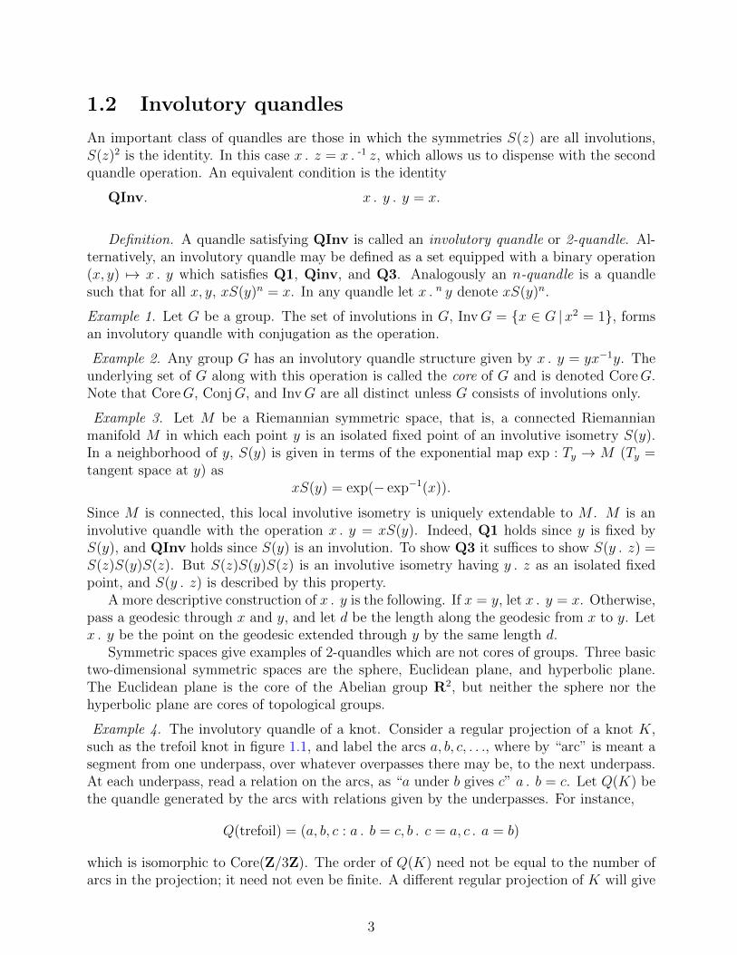
Example 4. The involutory quandle of a knot. Consider a regular projection of a knot K,such as the trefoil knot in figure 1.1, and label the arcs a, b, c, . . ., where by “arc” is meant asegment from one underpass, over whatever overpasses there may be, to the next underpass.At each underpass, read a relation on the arcs, as “a under b gives c” a . b = c. Let Q(K) bethe quandle generated by the arcs with relations given by the underpasses. For instance,

Q(trefoil) = (a, b, c : a . b = c, b . c = a, c . a = b)

which is isomorphic to Core(Z/3Z). The order of Q(K) need not be equal to the number ofarcs in the projection; it need not even be finite. A different regular projection of K will give

3

Figure 1.1: The trefoil knot

b

a . b = c

a

c . a = b

cb . c = a

the same Q(K) up to isomorphism. Moreover, if K and K ′ are equivalent knots, then Q(K)is isomorphic to Q(K). Proofs and precise definitions will be supplied in Chapter 4.

A similar construction gives the (non-involutory) quandle of a knot. An orientation of theknot is used to determine the relations. As expected, the knot quandle holds more informationabout the knot than the involutory knot quandle.

M. Takasaki [16] defined involutory quandles under the name “kei”. Takasaki’s motivationderives form the net (web) theory of Thomsen [17, 18]. This theory is described in the bookof Blaschke and Bol [2]. A similar geometric basis underlies Moufang’s [9] study of loops.Bruck [3] defined the core of a Moufang loop as the underlying set of the loop along with theoperation (x, y) 7→ yx−1y (example 2 above). See Chapter 3 more more on loop cores.

Loos discovered the intrinsic algebraic structure of symmetric spaces as explained in Loos[7, 8]. Not only are Riemannian symmetric spaces determined by their algebraic structure, butso are affine symmetric spaces. This allows Loos to define a symmetric space as a differentiableinvolutory quandle in which every point is an isolated fixed point of the symmetry throughit.

4

Chapter 2

Representations and the generalalgebraic theory of quandles

There are various ways that groups may be used to represent quandles. First of all, ConjG,for G a group, is a quandle. Many quandles may be represented as subquandles of ConjG forappropriate G. Free quandles, for example, may be so represented. Secondly, homogeneousquandles may be represented as cosets H\G for H a subgroup of G where an automorphism ofG fixing H is needed to describe the quandle operations on H\G. Non-homogeneous quandlesare representable as a union H1\G ∪ H2\G ∪ · · · where several automorphisms are used todescribe the quandle operations. Finally, a quandle may be given by a set Q along with anaction of a group G and a function ε : Q→ G that describes the symmetries of the points ofQ. Such a construction will be called an augmented quandle. We will be able to study somevarieties of quandles by means of augmented quandles.

2.1 The algebraic theory of conjugation

In this section we show that the theory of quandles may be regarded as the theory of con-jugation. Consider the two binary operations of conjugation, (x, y) 7→ y−1xy = x . y and(x, y) 7→ yxy−1 = x .-1 y, on a group. We ask whether there are any equations involving onlythese two operations which hold uniformly for all groups other than those which hold in allquandles. To this end we show that free quandles may be faithfully represented as unions ofconjugacy classes in free groups.

Proposition. Let A be a set and F be the free group on A. Then the free quandle on Aappears as the subquandle Q of ConjF consisting of the conjugates of the generators of F .

Proof. We use the notation of quandles in ConjF . Each element of Q is named as

a .e1 b1 .e2 · · · .en bn

where a, b1, . . . , bn ∈ A and e1, . . . , en ∈ 1,−1. That is to say, the conjugates of a are ofthe form

b−enn · · · b−e11 abe11 · · · benn .The equivalence on names is generated by two cases.

1. If a = b1, then a .e1 b1 .e2 · · · .en bn names the same element as a .e2 b2 .

e3 · · · .en bn.

5

2. If bi = bi+1 and ei + ei+1 = 0, then a .e1 b1 .e2 · · · .en bn names the same element as

a .e1 · · · .ei−1 bi−1 .ei+2 bi+2 . · · · .en bn.

Now let each a in A be assigned to a point f(a) in a quandle P . If f extends to Q, then wemust have

f(a .e1 b1 .e2 · · · .en bn) = f(a) .e1 f(b1) .

e2 · · · .en f(bn).

We must only show that this extension is well-defined. But this follows directly from the factthat in P the analogues of 1) and 2) hold for f(a) .e1 f(b1) .

e2 · · · .en f(bn).

Corollary. any equation holding in ConjG for all groups G holds in all quandles.

Proof. Let E be an equation holding in ConjG for all groups G. In particular E holds inConjF for free groups F , hence, E holds in free quandles. Whence, E holds in all quandles.

2.2 Automorphism groups of quandles

Let Q be a quandle. We define three automorphism groups for A. First, there is the groupconsisting of all automorphisms, the full automorphism group of Q, AutQ. Second, there isthe subgroup of AutQ, generated by all the symmetries of Q, called the inner automorphismgroup of Q, InnQ. Third, there is the subgroup of InnQ generated by automorphisms ofthe form S(x)S(y)−1 for x, y ∈ Q, called the transvection group of Q, TransQ. InnQ is anormal subgroup of AutQ, and TransQ is normal in both InnQ and AutQ. The quotientgroup InnQ/TransQ is a cyclic group. The elements of TransQ are the automorphisms ofthe form S(x1)

e1 · · ·S(xn)en such that e1 + · · ·+ en = 0.To illustrate these groups let Q be R2 with x . y = 2y − z considered as a quandle in

the category of topological spaces. Then AutQ consists of the continuous automorphisms ofR2, that is, the affine transformations. InnQ includes symmetries at points and translations.TransQ includes only translations.

2.3 Representation of quandles as conjugacy classes

Two points x and y of a quandle Q are said to be behaviorally equivalent if z . x = z . y forall z in Q. An equivalent condition is that S : Q → InnQ identifies x and y. Behavioralequivalence is a congruence relation, ≡b, on the quandle, and Q/ ≡b is isomorphic to theimage S(Q) as a subquandle of Conj InnQ. The elements of Q are behaviorally distinct ifand only if S is an injection, in which case Q is isomorphic to a union of conjugacy classesin InnQ.

Even if the points of a quandle are not all behaviorally distinct, the quandle may beisomorphic to a union of conjugacy classes of some group. For instance, any quandle satisfyingx . y = x may be embedded in Conj(

∏I Z2) for sufficiently large I. There is a universal group

in which to represent a quandle as a subset closed under conjugation. As noted in example 1of Chapter 1, every group G may be considered to be a quandle ConjG, with conjugation asthe quandle operation. Adjointly, every quandle Q gives rise to a group AdconjQ, generatedby the elements of Q modulo the relations of conjugation. Precisely, AdconjQ has the

6

presentation(x, for x ∈ Q : x . y = y−1x y, for x, y ∈ Q.

The map η : Q→ Conj AdconjQ sending x to x is a quandle homomorphism whose image isa union of conjugacy classes of AdconjQ. The map η has the following universal property:for any quandle homomorphism h : Q → ConjG, G a group, there exists a unique grouphomomorphism H : AdconjQ → G such that h = H η. Thus, if any h : Q → ConjG ismonic, then η is monic.

But η need not be injective in general. Consider the 2-quandle of three elements given

in the table in figure 2.1. Since b . a = b, a commutes with b. But a . b = c, so b−1ab = c.

Therefore, a = c, and η is not injective.

Figure 2.1: A singular 2-quandle

. a b ca a c ab b b bc c a c

Later, when we consider the quandle associated to a knot, the non-injectivity of η will beimportant. For example, the quandles associated to the square and granny knots are distinct,but the Adconj groups of these quandles (which are the knot groups) are isomorphic, and foreach, η is not injective.

2.4 Representation of quandles as cosets

Let s be an automorphism on a group G. We may define a quandle operation on G byx . y = s(xy−1)y. Verification is straightforward. Let H be a subgroup of G whose elementsare fixed by s. Then H\G inherits this quandle structure

Hx.Hy = Hs(xy−1)y.

Denote this quandle as (H\G; s). G acts on the right on (H\G; s) by (Hx, y) 7→ Hxy, andthe action is by quandle automorphisms. Since G acts transitively on H\G, it follows that(H\G; s) is a homogeneous quandle, that is, there is a quandle automorphism sending anypoint to any other point of the quandle.

We are mainly interested in the case when s is an inner automorphism of G, s(x) = z−1xzfor some fixed element z of G. Then x . y = z−1xy−1zy. When H contains z, the operationof (H\G; z) = (H\g; s) is

Hx.Hy = Hxy−1zy.

Proposition. Every homogeneous quandle is representable as (H\G; z).

Proof. Let Q be a homogeneous quandle and G = AutQ. Fix p ∈ Q. Let z = S(p),symmetry at p, and let s be conjugation by z in G. Then e : (G; s) → Q, evaluation atp, defined by sending the element x to its value at p, is a quandle homomorphism. Indeed,e(x . y) = e(z−1xy−1zy) = p xy−1zy = (p xy−1 . p)y = p xy−1y . py = e(x) . e(y). Since Q is

7

homogeneous, e is surjective. Let H be the stability subgroup of p, H = x ∈ G | px = p.Then e factors through (H\g; z) since p = pH. Moreover, (H\G; z) → Q is injective, forif pHx = pHy, then pxy−1 = p, xy−1 ∈ H, and so Hx = Hy. Thus, Q is isomorphic to(H\G; z).

Some adjustments are needed to represent non-homogeneous quandles. Given a groupG, elements z1, z2, . . . of G, and subgroups H1, H2, . . . of G such that for each index i, Hi iscontained in the centralizer of zi, we form a quandle (H1, H2, . . . \G; z1, z1, . . .) as the disjointunion of H1\G,H2\G, . . . with the quandle operation

Hix .Hjy = Hixy−1zjy.

Proposition. Every quandle is representable as (H1, H2, . . . \G; z1, z1, . . .).

Proof. Let Q be a quandle and G = AutQ. Let Q1, Q2, . . . be the orbits of the action of Gon Q. For each index i choose pi ∈ Qi, let zi = S(pI), and let Hi be the stability subgroupof pi. Then for each i, Hi is contained in the centralizer of zi, and so we have a quandleP = (H1, H2, . . . \G; z1, z1, . . .) as described above. Define e : P → Q by Hix 7→ pix. As inthe proof of the previous proposition, e may be shown to be an isomorphism.

In the case of involutory quandles, the automorphism s of G must be an involution on Gwhile the elements z, z1, z2, . . . of g must be involutions in G.

2.5 Algebraic connectivity

We say that a quandle Q is algebraically connected (or just connected when there will be noconfusion with topological connectivity) if the inner automorphism group InnQ acts transi-tively on Q. In other words, Q is connected if and only if for each pair a, b in Q there area1, a2, . . . , an in Q and e1, e2, . . . , en ∈ 1,−1 such that

a .e1 a1 .e2 · · · .en an = b.

Let Q be a quandle and q a point of Q. The q-fibre of a map g : Q→ Q′′ is the subquandleQ′ = p ∈ Q | g(p) = g(q) of Q. Suppose that Q′′ is a quotient of Q, that is, Q′′ is givenby a congruence on Q. In general the q-fibre does not determine Q′′; just consider quandleswhose operation is the first projection.

Proposition. Let Q be an algebraically connected quandle and q a point of Q. Then everyquotient of Q is determined by its q-fibre. Consequently, every congruence on Q is determinedby any one of its congruence classes.

Proof. Let Q′′ be a quotient of Q with q-fibre Q′. Let a, b ∈ Q. By the connectivity of Qthere is an inner automorphism x such that ax = q. Since homomorphisms respect innerautomorphisms, it follows that g(a) = g(b) if and only if g(ax) = g(bx). Hence, g(a) = g(b)if and only if ∃x ∈ InnQ such that ax = q and bx ∈ Q′. Thus, Q′ determines Q′′.

8

2.6 The transvection group

As defined above, the transvection group TransQ of a quandle Q is the subgroup of InnQgenerated by automorphisms of the form S(x)S(y)−1. TransQ is a normal subgroup of InnQwith cyclic quotient. Alternatively, we may define a transvection on Q as an automorphism ofQ of the form S(x1)

e1 · · ·S(xn)en with xi ∈ Q, ei ∈ Z, i = 1, . . . , n, such that e1+ · · ·+en = 0.Then TransQ is the group of transvections on Q.

Some the the properties of Q are reflected in TransQ.

Proposition. A quandle is Abelian if and only if its transvection group is Abelian.

Proof. Let Q be a quandle with transvection group T . By definition, Q is Abelian if and onlyif

(w .x) .(y . z) = (w . y) .(x . z).

Equivalently,S(x)S(z)−1S(y) = S(y)S(z)−1S(x).

On the other hand, T is Abelian if and only if

S(x)S(z)−1S(y)S(t)−1 = S(y)S(t)−1S(x)S(z)−1.

By setting t = z we find that if T is Abelian then Q is Abelian. From Q Abelian follows

S(x)S(z)−1S(y)S(t)−1 = S(y)S(z)−1S(x)S(t)−1

= S(y)S(t)−1S(x)S(z)−1.

which implies that T is Abelian.

2.7 n-Cores

The core of a group has the property that all its symmetries are involutions. In this sectionwe define an n-core of a group wherein the n-th power of each symmetry is the identity. Thisagrees with the usual core in the case n = 2.

LetG be a group and n a positive integer. The wreath productGoZn consists of n+1-tuples(x0, . . . , xn−1, k) with xi ∈ G, k ∈ Zn. The index i is to take values in Zn. Multiplication inG o Zn is given by

(x0, . . . , xn−1, k) · (y0, . . . , yn−1, l) = (x0yk, x1yk+1, . . . , xn−1yk−1, k + l).

Let Q be the conjugacy class of (1, . . . , 1, 1) in G o Zn. Then

Q = x0, . . . , xn−1, 1) |x0 · · ·xn−1 = 1

and the quandle operation on Q is given by

(x0, . . . , xn−1, 1) .(y0, . . . , yn−1, 1) = (y−1n−1xn−1y0, y−1) x0y1, . . . , 1).

This quandle is called the n-core of G. The 2-core of G is isomorphic to the core of G.

9

2.8 Examples of simple quandles

A quandle is said to be simple if its only quotients are itself and the one-point quandle.We will show in this section that n-cores of noncyclic simple groups are simple. In fact, anoncyclic group is simple if and only if its n-core is simple. Also, nontrivial conjugacy classesof simple groups are simple. We proceed with some lemmas.

Lemma 1. Let H be a group with commutator H ′. An element x in H lies in H ′ if and onlyif there exist x1, x2, . . . , xk in H such that x = x1x2 . . . xk and xk . . . x2x1 = 1.

Lemma 2. Let H be a perfect group, H = H ′. Then the n-core Q of H as a subset ofG = H o Zn generates G.

Proof. Let b = (1, 1) = (1, . . . , 1, 1) ∈ Q. Let x ∈ H. By lemma 1, x = x1 . . . xk, xk . . . x1 = 1.Then

(x1, x−11 , 1, . . . , 1)b−1(x2, x

−12 1, . . . , 1)b−1 . . . (xk, x

−1k , 1, . . . , 1)b−1

= (x1x2 · · ·xk, x−11 x−12 · · ·x−1k , 1, . . . , 1, 0)

= (x, 1, . . . , 1, 0).

Since b and each (xi, x−1i , 1, . . . , 1) lie in Q, so (x, 1, . . . , 1, 0) is a member of the subgroup

generated by Q. The rest follows easily.

Lemma 3. If the center of a nontrivial group H is trivial, then the center of H oZn is trivial.

Lemma 4. Let G be a group with trivial center, and let Q be a conjugacy class that generatesG. Then G ∼= InnQ, and G′ ∼= TransQ.

Proof. For each x ∈ G let S(x) be conjugation by x, and regard S(x) as an automorphism ofQ. Then S is a group homomorphism S : G→ AutQ. Note that S(x) = 1 if and only if forall q in Q, x−1qx = q. Since Q generates G, S(x) = 1 if and only if x ∈ Z(G). Therefore, Sis injective. The image of S is InnQ. Hence, S is an isomorphism G ∼= InnQ.

We show next that S(G′) = TransQ. Let p, q ∈ Q. Then [S(p), S(q)] = S(p)−1S(p . q) ∈TransQ. TransQ is a normal subgroup of InnQ, so S(G′) = (InnQ)′ ⊆ TransQ. Since Qis a conjugacy class in G, there is an x in G such that x−1px = q. Therefore, S(p)−1S(q) =[x, S(q)] ∈ (InnQ)′. Thus, TransQ ⊆ S(G′).

Lemma 5. Under the hypotheses of lemma 4 the following statements are equivalent.

(1) Q is a simple quandle.

(2) G′ is the smallest nontrivial normal subgroup of G.

(3) G′ is a minimal nontrivial normal subgroup of G.

Proof. (1) =⇒ (2). Let N be a normal subgroup of InnQ. Define an equivalence relation onQ by

p ≡ q ⇐⇒ ∃n ∈ N such that pn = q.

We show that ≡ is an congruence. Assume p ≡ q, pn = q. For r in Q we have q . r = pn . r =(p . r)m where m = S(r)−1nS(r) ∈ N . Hence, q . r ≡ p . r. Also r . q = r . pn = (r . p)m−1nwhere m−1n ∈ N . Hence, r . q = r . p. Therefore, ≡ is a congruence. By the simplicity of Qwe have only two cases.

10

Case 1. ≡ is equality. Let n ∈ N . For all q in Q, qn = q, so n−1S(q)n = S(q). From thehypotheses of the lemma it follows that n = 1. Thus, N = 1.

Case 2. ≡ relates all points of Q. For p, q in Q there is an n in N such that pn = q. Thenn−1S(p)n = S(q). Therefore, S(p)S(q)−1 ∈ N . Hence, TransQ ⊆ N .

Now (2) follows from the conclusions of lemma 4.

(2) =⇒ (3). Clear.

(3) =⇒ (1). Assume (3). Let ≡ be a congruence on Q. Conjugation by elements of Qrespects ≡, that is, p ≡ q implies p . r ≡ q . r. Since Q generates G, conjugation by elementsof G respects ≡. Let

N = x ∈ G′ | ps(x) ≡ p for all p ∈ Q.Then N is a normal subgroup of G contained in G′. By (3), either N = 1 or N = G′. Assume≡ is not equality. Then ∃q, r ∈ Q such that q ≡ r but q 6= r. It follows that 1 6= qr−1 ∈ N .Hence, N = G′. Now let q, r be arbitrary in Q. ∃x ∈ G′ such that x−1qx = r. Therefore,q ≡ qS(x) = p. Thus, if ≡ is not equality, then ≡ relates any two elements.

Lemma 6. Let H be a noncyclic simple group and G = H o Zn, n ≥ 2. Then K =(x0, . . . , xn−1, 0) ∈ G is a minimal nontrivial normal subgroup of G.

Proof. Let (x0, . . . , xn−1, 0) be a nontrivial element of K. We will show the smallest normalsubgroup N containing this element is K. For some i, xi 6= 1, say i = 0. There is an elementw of G such that [x0, w] = z 6= 1. Then [(x0, . . . , xn−1, 0), (w, 1, . . . , 1)] = (z, 1, . . . , 1, 0) liesin N . As z 6= 1 and H is simple, it follows that (y, 1, . . . , 1, 0) ∈ N for all y in H. Now

(y, 1, . . . , 1, 0) .(1, . . . , 1, k) = (1, . . . , y, . . . , 1, 0)

also lies in N for all y in H and k in Zn. Hence N = K.

Theorem 1. Let H be a noncyclic group and Q be the n-core of H (n ≥ 2). Then Q is simpleif and only if H is simple, in which case InnQ ∼= G = H o Zn and

TransQ ∼= G′ = (x0, . . . , xn, 0) ∈ G ∼= Hn.

Proof. Assume H is simple. According to lemma 2, Q generates G, and by lemma 3 z(G) = 1.Since the hypotheses of lemma 4 hold, we have G ∼= InnQ, and G′ ∼= TransQ. Lemma 6 saysK = (x0, . . . , xn−1, Q) ∈ T is a minimal nontrivial normal subgroup of G. Hence, G′ = K.Finally, we conclude from lemma 5 that Q is simple.

Any normal subgroup N of H gives a quandle congruence on Q defined by

(x, 1) ≡ (y, 1) ⇐⇒ xiy−1i ∈ N for i = 0, . . . n− 1.

Moreover, if N 6= 1, then ≡ is not equality. Hence, the simplicity of Q assures that of H.

The n-core of a noncyclic simple group retains, therefore, more information about thegroup than just its simplicity. It can, in fact, be reconstructed from its n-core.

Remark. The 4-core of the cyclic simple group Z2 is not a simple quandle.

Corollary. The core (2-core) of a group is simple if and only if the group is simple.

Proof. The only groups not covered by the theorem are cyclic groups for which the statementis easily verified.

11

There are two other ways that simple quandles derive from simple groups besides n-cores.We will show that any nontrivial conjugacy class in a simple group is a simple quandle. Thefollowing lemma is a direct consequence of lemmas 4 and 5.

Lemma 7. Under the hypotheses of lemma 4, if G′ is a simple group, then Q is a simplequandle.

Theorem 2. Let H be a noncyclic simple group and Q a nontrivial conjugacy class in H.Then Q is a simple quandle. Also, InnQ = TransQ ∼= H.

Proof. Q generates H, and z(H) = 1. So by lemma 4, InnQ = TransQ ∼= H. By lemma 7,Q is a simple quandle.

Theorem 3. Let H be a noncyclic simple group, p a prime integer, and s an outer automor-phism of G of order p. Let G be the semidirect product HnZp, (x, y)·(y, l) = (xs−k(y), k+l).Then Q is a simple quandle, InnQ ∼= G, and TransQ ∼= H.

Proof. First we show that Q generates G. Let (Q) be the subgroup generated by Q. (Q) isnormal in G. (1, 1) ∈ (Q), so (1, k) ∈ (Q) for all k in Zp. Also, (1, 1) .(y, 0) = (y−1s−1(y), 1) ∈(Q). Since s 6= 1, ∃y ∈ H such that 1 6= (y−1s−1(y), 1) ∈ (Q). Also (y−1s−1(y), 0) ∈ (Q).Hence (Q) ∩H 6= 1. Therefore, (Q) ∩H = H. It follows that (Q) = G.

Next we show Z(G) = 1. Suppose (a, k) ∈ Z(G). Then zs−k(y) = yz for all y in H. Thus,sk = S(z−1). If p divides k, then 1 = sk = S(z−1), which gives (z, k) = (1, 0). Otherwise,(p, k) = 1. Then for some m, km ≡ 1 mod p, so s = skm = S(z−m). in contradiction to thehypothesis that s is not an inner automorphism. This, Z(G) is trivial.

We have shown that Q and G satisfy the hypotheses of lemma 4. Hence, G ∼= InnQ, andG′ ∼= TransQ.

Clearly, G′ = H n 0 ∼= H, so by lemma 7, Q is simple.

2.9 Classification of simple p-quandles

In this section we examine the problem of classifying simple quandles. In the case of p-quandles, p a prime integer, we solve the problem in terms of simple groups. Throughoutthis section let Q be a simple quandle and G = InnQ.

Lemma 1. Either S : Q→ G is injective or the order of Q is less than three.

Proof. The behavioral equivalence on Q is either equality or else relates any two elements ofQ. In the former case S is injective. In the latter case Q satisfies the identity x . y = x. Butthe only simple quandles satisfying x . y = x have fewer than three elements.

Assume for the rest of this section that the order of Q is greater than two. Since the setof connected components of Q is a quotient of Q, it follows that Q is algebraically connected.Also, S(Q) is a conjugacy class in G since it is closed under conjugation and generates G.

Lemma 2. The center of G is trivial.

Proof.

z ∈ Z(G) ⇐⇒ ∀q ∈ Q, zS(q) = S(q)z

⇐⇒ ∀q ∈ Q,S(qz) = S(q)

⇐⇒ ∀q ∈ Q, qz = q.

12

But the only automorphism fixing all the points of Q is 1. Therefore, Z(G) = 1.

By lemma 4 of section 2.9 we have TransQ = G′. Hence, G/G′ is a cyclic group. Moreover,if Q is an n-quandle, then the order of G/G′ divides n. Since S(Q) ∼= Q is a simple quandle,by lemma 5 of section 2.9 it follows that G′ is the smallest nontrivial normal subgroup of G.

At this point we must break the classification into cases. If G′ = G, then G is a simplegroup, and Q is isomorphic to the nontrivial conjugacy class S(Q) in the simple group G.For the rest of this section we assume G′ 6= G. We will also assume that Q is a p-quandle, pa prime integer. Then G/G′ ∼= Zp.

Fix q0 in Q. Let x0 = S(q0) ∈ G, and let s be conjugation by x0 as an automorphism ofG′. Then x0 6= 1, xpo = 1, s 6= 1, sp = 1. Let K be the semidirect product G′ n Zp where

(x, k)(y, l) = (xs−k(y), k + l).

There is an isomorphism f : K → G, f(x, k) = xxk0. In particular, f(1, 1) = x0, andf−1(S(Q)) is the conjugacy class in K of (1, 1).

Suppose G′ is a simple group. From the fact that Z(G′) = 1 it follows that s is not an innerautomorphism of G′. Thus, Q is isomorphic to the conjugacy class of (1, y) in k = G′ n Zp

where G′ is a simple group and G′ n Zp is constructed from an outer automorphism of G′ oforder p. This is the situation encountered in theorem 3 of section 2.8.

We have yet to consider the case where G′ is not simple.

Lemma 3. Let H be a group with a smallest nontrivial normal subgroup T such that [H :T ] = p is prime. Assume T is not simple. Then T is isomorphic to Np for some simple groupN .

Proof. Let N be a nontrivial proper normal subgroup of T . Fix x in H − T . Let s beconjugation by x as an automorphism of T . Then sp(N) = N since xp ∈ T . More generally,sp+i(N) = si(N) for any integer i. Since p is prime and N is not normal in N , we have pdistinct conjugates of N , namely,

N, s(N), . . . , sp−1(N).

Claim. For k = 0, 1, . . . , p − 2, there exist nontrivial proper normal subgroups Nk of Tsuch that 0 6= |i− j| ≤ k implies si(Nk) ∩ sj(Nk) = 1.

Define N0 = N . Inductively define Nk+1 (k + 1 ≤ p− 1) as follows. The group

Nk ∩ sk+1(Nk) ∩ · · · ∩ s(k+1)(p−1)(Nk)

is normal in G since k + 1 is relatively prime to p, and, being strictly containedin T , is, therefore, trivial. Let l be least such that

Nk ∩ sk+1(Nk) ∩ · · · ∩ s(k+1)l(Nk) = 1.

ThenNk+1 = Nk ∩ sk+1(Nk) ∩ · · · ∩ s(k+1)(l−1)(Nk)

satisfies the requirements of the claim.

13

We may assume N = Np−1. That is, the p conjugates of N ,

N, s(N), . . . , sp−1(N),

have pairwise trivial intersection and generate T . Hence

T = N × s(N)× · · · × sp−1(N) ∼= Np.

Also, N is simple. Indeed, if M is a proper normal subgroup of N , then M × s(M)× · · · ×sp−1(M) is normal in H and strictly contained in T and, therefore, is trivial as is M .

Theorem 1. Let Q be a simple p-quandle, p a prime, and let G = InnQ. As noted above,G′ = TransQ. Assume G′ is not a simple group. Then G is a wreath product of a simplegroup N with Zp, G

′ ∼= Np, and Q is isomorphic to the p-core of N .

Proof. By lemma 3, G′ ∼= Np where N is a simple group. As noted above G is isomorphic toG′ n Zp. Therefore, G = G′ n Zp = N o Zp. Also, Q is isomorphic to the conjugacy class of(1, 1) in G′ n Zp and, therefore, to the p-core of N .

Scholium. simple p-quandles of order greater than two arise in three ways:

1. a nontrivial conjugacy class in a simple group,

2. the conjugacy class of (1, 1) in H n Zp where H is a simple group and H n Zp isconstructed from an outer automorphism of H,

3. the p-core of a simple group.

The three cases are distinguished by the structure of the inner automorphism group of thequandle.

2.10 Augmented quandles

Let G be a group acting on a quandle Q by quandle automorphisms. That is, for x, y ∈ Gand p, q ∈ Q we have

q(xy) = (qx)y, and

(p . q)x = px . py.

Assume that G contains representatives of the symmetries of Q, that is, there is a functionε : Q→ G satisfying

pε(q) = p . q.

In particular, we have

AQ1. pε(p) = p, for p ∈ Q.Assume further that ε satisfies the coherency condition

AQ2. ε(px) = x−1ε(p)x, for p ∈ Q, x ∈ G.Then we have a group action on Q, Q × G → Q, and a function ε : Q → G which satisfyAQ1 and AQ2.

14

Conversely, given a group action of G on a set Q, Q×G→ Q, and a function ε : Q→ Gsatisfying AQ1 and AQ2, we can define quandle operations on Q as x . y = xε(y) andx .-1 y = xε(y)−1 so that the action of G on Q is by quandle automorphisms.

Definition. An augmented quandle (Q,G) consists of a set Q and a group G equipped witha right action on the set Q and a function ε : Q → G called the augmentation map whichsatisfy AQ1 and AQ2.

With the operations mentioned above Q is a quandle, and the augmentation map is aquandle homomorphism ε : Q→ ConjG.

A morphism of augmented quandles from (Q,G) to P,H) consists of a group homomor-phism g : G→ H and a function f : Q→ P such that the diagram

Q×G −−−→ Qε−−−→ G

f×gy f

y g

yP ×H −−−→ P

ε−−−→ H

commutes. It follows that f is a quandle homomorphism.

Examples. Fix a quandle Q. Two examples of augmented quandles with underlying quandleQ are (Q,AutQ) and (Q, InnQ). the augmentation in each case is the function that has beendenoted S. The action is the natural one. In the category of augmentations of Q, (Q,AutQ)is the terminator. That is, for each augmentation (Q,G), there is a unique homomorphismf : G→ AutQ such that

Q×G −−−→ Qε−−−→ G

1×fy 1

y f

yQ× AutQ −−−→ Q

S−−−→ AutQ

commutes. The map f is readily defined from Q×G→ Q.Another example of an augmentation of Q is (Q,AdconjQ), (see section 2.3). The function

representing symmetries of Q is η : Q→ AdconjQ, while the group action is defined by

z(ye11 · · · yenn ) = z .e1 y1 .e2 · · · .en yn,

where z ∈ Q and ye11 · · · yenn is an arbitrary element of AdconjQ, yi ∈ Q, ei ∈ −1, 1 fori = 1, . . . n. To show that this is a well-defined group action, it suffices to note that

z(x . y) = x .(x . y)

= z .−1 y . x . y

= zy−1x y

The axiom AQ1 clearly holds. Since η(Q) generates AdconjQ, AQ2 reduces to the fact thatη : Q→ Conj AdconjQ is a quandle homomorphism as noted in section 2.3.

In the category of augmentations of Q, (Q,AdconjQ) is the coterminator. That is, foreach (Q,G) there is a unique group homomorphism f : AdconjQ→ G such that

Q× AdconjQ −−−→ Qη−−−→ AdconjG

1×fy 1

y f

yQ×G −−−→ Q

ε−−−→ G

15

commutes. According to the right square, f must be the map H : AdconjQ → G describedin section 2.3. To show the commutativity of the left square it suffices to show zy = zf(y)for y, z in Q, since such y generate AdconjQ. But zy = z . y = zε(y) = zf(y).

We consider now constructions in the category AQ of augmented quandles. Products,equalizers, and limits in general are of the usual sort. For instance, the product of (Q,G)and (P,H) has as its augmentation group G×H and has as its underlying quandle Q× P .However, it will take more work to describe colimits.

Let U be the forgetful functor from AQ to the category of groups, U(Q,G) = G. Uhas both a left adjoint T and a right adjoint V . That U has a left adjoint T is automaticand uninteresting. T (G) = (∅, G). On the other hand, the existence of a right adjoint Vis unexpected. Let G be a group. Then V (G) = (ConjG,G) where G acts on ConjG byconjugation and the function ε : ConjG → G is the identity. We show that (ConjG,G)satisfies the appropriate universal property. Let (G,H) be an augmented quandle and f :H → G a group homomorphism. We must show there exists a unique function g : Q→ ConjGsuch that

Q×H −−−→ Qε−−−→ H

g×fy g

y f

yConjG×G −−−→ ConjG −−−→ G

commutes. Since ConjG→ G is the identity, the function g must be f ε. The commutativityof the left square states

(∗) g(qx) = g(q) · f(x)

for q ∈ Q, x ∈ H. Here, g(q) · f(x) denotes conjugation of g(q) by f(x), so equalsf(x)−1g(q)f(x) where the multiplication occurs in G. Then (∗) is equivalent to

f ε(qx) = f(x)−1(f ε)(q)f(x)

= f(x−1ε(q)x),

and this follows from axiom AQ2 for (Q,H).The existence of a right adjoint for U simplifies the construction of colimits in AQ. If

(Q,G) is the colimit, lim←−(Qi, Gi), then G is the colimit, lim←−Gi, in the category of groups.Unfortunately, the forgetful functor from AQ to the category of quandles has no right adjoint.We need another construction of augmented quandles to describe their colimits.

Let (Q,G) be an augmented quandle and f : G → H a group homomorphism. ThenQ×H is a right H-set with action (q, x)y = (q, xy) for q in Q and x, y in H. Define an H-setcongruence on Q×H by (q, y) ≡ (p, z) if and only if yz−1 = f(x) and p = qx for some x ∈ G.Let q⊗y denote the congruence class of (q, y), and let Q⊗GH, or more simply Q⊗H, denotethe set of congruence classes. We have

(q ⊗ y)z = q ⊗ yz, and

q ⊗ f(x) = qx⊗ 1.

Define ε : Q ⊗ H → H by ε(q ⊗ x) = x−1(f ε)(q)x. ε is well-defined since axiom AQ2holds for (Q,G). Then (Q⊗H,H) is an augmented quandle, as can be directly verified. Wealso have a function i : Q → Q ⊗ H given by q 7→ q ⊗ 1, which along with f gives a map(i, f) : (Q,G)→ (Q⊗H,H) of augmented quandles.

16

Proposition. Let (Q,G) be an augmented quandle and f : G → H a group homomorphism.Then (i, f) : (Q,G) → (Q ⊗ H,H) satisfies the following universal property. For each mapof the form (g, h f) : (Q,G) → (P,K), there exists a unique map of the form (k, h) :(Q⊗H,H)→ (P,K) such that (g, h f) = (k, h) (i, f). Otherwise said, in the category ofaugmented quandles

(∅, G) −−−→ (Q,G)

(1,f)

y y(i,f)

(∅, H) −−−→ (Q⊗H,H)

is a pushout diagram.

Proof. Let (g, h f) : (Q,G) → (P,K) be given. Denote the required function Q ⊗H → Pby k. There are four requirements on k. In order that k be well-defined we need

1) k(q ⊗ f(x)y) = k(qx⊗ y), for q ∈ Q, x ∈ G, y ∈ H.

In order that (k, h) be a map in AQ we need

2) (ε k)(q ⊗ y) = (h ε)(q ⊗ y), for q ∈ Q, y ∈ H,

and

3) k(q ⊗ yz) = k(q ⊗ y)h(z), for q ∈ Q, y, z ∈ H.

And so that (q, h f) = (k, h) (i, f) we need

4) g(q) = k(q ⊗ 1), for q ∈ Q.

Together, 3) and 4) show that k must be defined as k(q ⊗ y) = g(q)h(y), giving theuniqueness of k. With this definition of k, 1) states

g(q)h(f(x)y) = g(qx)h(y).

This reduces tog(q)(h f)(x) = g(qx),

which holds since (g, h f) is a map in AQ.Finally, 2) states that

ε(g(q)h(y)) = (h ε)(q ⊗ y).

But

ε(g(q)h(y) = h(y)−1(ε g)(q)h(y)

= h(y)−1(h f ε)(q)h(y)

= h(y−1(f ε)(q)y)

= (h ε)(q ⊗ y).

We will denote the function k in the proposition by g in spite of the confusion it maycause. In this notation (g, hf) = (g, h) (i, f). In the case that H = K and h is the identityfunction, 1 : H → H, we have (g, f) = (g, 1) (i, f). Note also that when H = G and f is

17

the identity, 1 : G→ G, then the augmented quandle (Q⊗G G,G) is the original augmentedquandle (Q,G). Hence, Q⊗G G = Q.

We now consider an arbitrary colimit (Q,G) = lim←−(Qj, Gj) in the category AQ. As notedabove G is the colimit, lim←−Gj, in the category of groups. By the preceding proposition, foreach j, (Qj, Gj) → (Q,G) factors uniquely through (Qj, Gj) → (Pj, G) where Pj denotesQj ⊗Gj

G. Consequently, (Q,G) ∼= lim←−(Pj, G). This reduces the construction of colimits tothe case where a single group G acts on all the sets Pj, and all maps (Pj, G) → (Pk, G) areof the form (f, 1).

In this case let P = lim←−Pj in the category of sets. Then P has a unique right G-actiondetermined by the G-actions on the Pj, so we might just as well have taken this colimitin the category of G-sets. There is also a function ε : P → G determined by the functionsε : Pj → G. It may be directly verified that with this action and ε that (P,G) is an augmentedquandle. By the definition of P there is a unique function (f, 1) : (P,G)→ (Q,G) determinedby the maps (Pj, G)→ (Q,G). Also the function (f, 1) satisfies the commutativity conditionsto be a map in AQ since all the maps (Pj, G)→ (Q,G) satisfy these conditions. Furthermore,all the maps (Pj, G)→ (P,G) lie in AQ, so (P,G) = lim←−(Pj, G).

We summarize these results.

Theorem. A colimit, lim←−(Qj, Gj) in AQ is isomorphic to lim←−(Qj ⊗GjG,G) where G = lim←−Gj

in the category of groups. It is also isomorphic to (lim←−Qj ⊗GjG,G) with lim←−Qj ⊗Gj

G takenin the category of sets.

2.11 Quotients of augmented quandles described by

normal subgroups of the augmentation group

Let (Q,G) be an augmented quandle and N be a normal subgroup of G. Let G denotethe quotient group G/N with elements denoted by x for x in G. Let Q and Q/N denotethe quandle Q ⊗G G. The elements of Q are equivalence classes q of elements of Q whereq = qn ∈ Q |n ∈ N. The action Q × G → Q is given by q x = qx and the augmentationε : Q→ Q is given by ε(q) = ε(q).

Let (Q,G) be an augmented quandle. In order that the quandle Q be Abelian we need

(p . q) .(r . s) = (p . r) .(q . s).

Equivalently, ε(q)ε(rε(s)) = ε(r)(ε(p)ε(s)). That is, every element in G of the form

(∗) ε(q)ε(s)−1ε(r)ε(q)−1ε(s)ε(r)−1

equal 1. Let N be the normal subgroup of G generated by such elements. Then the quotient(Q,G) of (Q,G) is assured to be Abelian. It is evident that (Q,G) has the universal propertythat each map (Q,G)→ (P,H) factors uniquely through (Q,G)→ (Q,G) whenever p is anAbelian quandle.

Proposition 1. Let (Q,G) be an augmented quandle such that ε(Q) generates G. Let N and(Q,G) be defined as above. Then Q is the Abelianization of the quandle Q.

Proof. Let P be an Abelian quandle and f : Q→ P be a quandle homomorphism. We mustshow that f : Q → P given by f(q) = f(q) is well defined, that is, f(qn) = f(q) for n ∈ N .

18

If n is of the form (∗), then f(qn) = f(q) since P is Abelian. Since G is generated by ε(Q)we may assume n is of the form ε(p)−1n′ε(p) where f(q′n′) = f(q′) for all q′ in Q. Then

f(qn) = f((q .-1 p)n′ . p)

= f((q .-1 p)n′) . f(p)

= f(q .-1 p) . f(p)

= f(q).

Thus, f is well-defined on Q.

Corollary 1. Let A be a set and G the group generated by A modulo relations ab−1c = cb−1afor conjugates a, b, c of the generators of G. Then the free Abelian quandle on A consists ofthe conjugates of the generators of G.

What has been done here for Abelian quandles can be done for many other varieties ofquandles. The method works for any variety defined by equations of the form

p .e1 ϕ1 .e2 · · · .em ϕm = p .f1 ψ1 .

f2 · · · .fn ψn

where the ϕi and ψj are expressions not involving p. For example, the identity for n-quandles,p .n q = p, is of this form.

Proposition 2. Let (Q,G) be an augmented quandle such that ε(Q) generates G, and N bea positive integer. Let Nn be the normal subgroup of G generated by ε(q)n for q in Q. ThenQ/Nn is the largest quotient of Q which is an n-quandle

Corollary 2. Let A be a set and G = (a, a ∈ A : an = 1, a ∈ A). The free n-quandle on Aconsists of the conjugates of the generators of G.

Corollary 3. The free involutory quandle on two points is isomorphic to Core Z with generators0 and 1.

Proof. Let A = a, b and G = (a, b : a2 = b2 = 1). Let Q be the quandle of conjugates of aand b in G. Let x = ab. Then G = (a, x : a2 = 1, axa = x−1). Each element of G is uniquelyrepresented as aexk with k ∈ Z and e ∈ 0, 1. The conjugates of a and b are those elementsof the form axk, k ∈ Z. Q = axk | k ∈ Z. Verification that axn . axm = ax2n−m yields anisomorphism of quandles f : Q→ Core Z, f(axn) = n. Also, f(a) = 0, f(b) = 1.

Proposition 3. The free Abelian involutory quandle on n+ 1 generators appears as

A = (k1, . . . , kn) ∈ Zn | at most one ki is odd

as a subquandle of Core Zn with generators e0 = (0, . . . , 0), e1 = (1, 0, . . . , 0), e2 =(0, 1, 0, . . . , 0), . . . , en = (0, . . . , 0, 1).

Proof. Let G be the group presented as

(ao, ..., an : a2i = 1, aiajak = akajai, all i, j, k),

and let Q include the conjugates of the generators of G. Then Q is the free Abelian involutoryquandle on a0, . . . , an. As A is an Abelian quandle, there is a unique map h : Q → A suchthat h(ai) = ei, i = 0, . . . , n. We will show h is an isomorphism. Let tj = aoaj, j = 0, . . . , n.

19

Then tjtk = tktj. The conjugates of ai are of the form ai . aj1 . · · · . ajr = ai . aj1 · · · ajr ,and r may be taken to be even since ai . ai = ai. Then ai . aj1 · · · ajr = ai . t

−1j1tj2 · · · t−1jr−1

tjr .

Thus, Q consists of elements of the form ai . tk11 · · · tknn with ki ∈ Z, i = 1, . . . , n. Now

h(ai . tk11 · · · tknn = ei + 2k1(e1 − e0) + 2k2(e2 − e0) + · · · + 2kn(en − e0) = ei + (2k1, . . . , 2kn).

Clearly, h is surjective and injective.

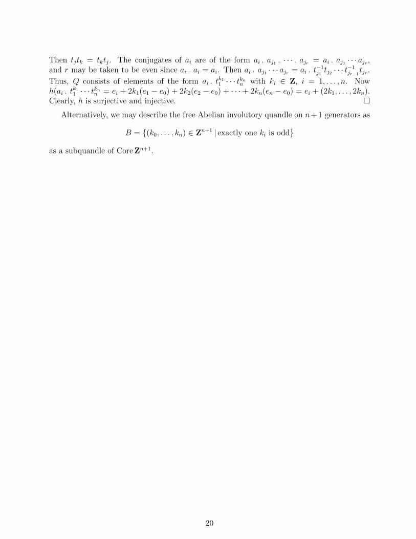
Alternatively, we may describe the free Abelian involutory quandle on n+ 1 generators as

B = (k0, . . . , kn) ∈ Zn+1 | exactly one ki is odd

as a subquandle of Core Zn+1.

20

Chapter 3

Involutory quandles

3.1 Involutory quandles and geodesics

The fact that symmetric spaces are involutory quandles and that their structure is determinedby distance along geodesics suggests that involutory quandles in general be determined bysome kind of geodesic. Consider, for example, the integral line quandle, L = Core Z. InterpretL as the integral points on a line. Then for m,n ∈ L, m.n is found by moving along theline from m through n the same distance beyond n as m is beyond n.

The suggestion may be formalized as follows. Define an involutory quandle with geodesicsas a set Q of points with a collection of functions, called geodesics, g : L→ Q, where L is theintegral line quandle Core Z, satisfying three axioms

QG1. Every pair of points lies in the image of some geodesic.

QG2. Whenever a pair of points x, y lie in the image of two geodesics, f(m) = x,f(n) = y, g(m′) = x, g(n′) = y, it is the case that f(m.n) = g(m′ . n′). Wedenote this point f(m.n) as x . y.

QG3. A geodesic reflected through a point is a geodesic; precisely, if x is a pointand f a geodesic, then there exists a geodesic g such that for all m,n ∈ L, thereexist p, q ∈ L such that f(m) . x = g(p), f(n) . x = g(q), and f(m.n) . x =g(p . q). See figure 3.1.

Figure 3.1: QG3

fqf(m) qf(n) qf(m.n)

gqg(p . q)

qg(q)

qg(p)

@

@@@@@@@

q x

21

It is easily seen that an “involutory quandle with geodesics” is an “involutory quandle”. Theoperation . is as defined in QG2.

Proposition. Every involutory quandle is representable as an involutory quandle withgeodesics.

Proof. Recall corollary 3, section 2.11, which states that L is the free involutory quandle ontwo points. Let Q be the given quandle. For each pair of points x, y in Q there is a uniquequandle map f : L→ Q such that f(0) = x and f(1) = y. Take all such maps as geodesics.Clearly, QG1 holds. For points x, y, if f is a geodesic such that f(m) = x and f(n) = y, thenf(m.n) = x . y, hence, QG2 holds. Finally, given a geodesic f and a point x, the geodesicg required for QG3 is that such that g(0) = f(0) . x and g(1) = f(1) . x.

Example. Figure 3.2 displays a 2-quandle by means of geodesics. Note that some pairsof points of the quandle lie on distinct geodesics. This particular example is algebraicallyconnected but does not have behaviorally distinct elements.

Figure 3.2: Geodesics

r

rr

r

r r

rr

r rr

r

3.2 Involutory quandles generated by two points

At this point it is appropriate to classify the involutory quandles generated by two points.They will all be quotients of the free involutory quandle on two points, L = Core Z.

Proposition. Any involutory quandle generated by two points is isomorphic to one of thefollowing

i). L = Core Z.

ii). C(n) = Core Zn, the (nonsingular) cyclic quandle of order n.

iii). Cs(4n), the quotient of C(4n) given by the congruence 2k ≡ 2k + 2n for allk ∈ Zn, the singular cyclic quandle of order 3n.

22

Figure 3.3: Singular quandles Cs(4) and CS(8)

q3 q 0 ≡ 2 q1Cs(4)

q 0 ≡ 4

q1

q3

q2 ≡ 6 q5q 7

Cs(8)

Remark. Figure 3.3 illustrates Cs(4) and Cs(8).

Proof. It is straightforward to check that the list induces only quotient quandles of L. Assumenow that Q is the proper quotient of L, Q = L/ ≡. Let d be the least difference betweenany two distinct equivalent points of L. d = |m − n| 6= 0, m ≡ n. By using a translationby −m on L, which is an isomorphism of L, we may assume m = 0. d = |n| 6= 0. Now−n = n . 0 ≡ 0 . 0 = 0, so 0 ≡ d. For all k, k = −k . 0 ≡ −k . d = k + 2d. Therefore, Q is aquotient of C(2d) = Core Z2d. Note that for all k, 2k = 0 . k ≡ d . k = 2k − d. Similarly,

(∗) 2k − d ≡ 2k ≡ 2k + d.

We consider two cases depending on the parity of d.

Case 1. d is odd. We show p ≡ p + d for all p. If p is even, p = 2k, then (∗) impliesp ≡ p+d. If p is odd, p = 2k−d, then (∗) implies p ≡ 2k ≡ p+d. Therefore, Q is a quotientof C(d) = Core Zd. By the minimality of d, Q = C(d).

Case 2. d is even. Let d = 2c. We see from (∗) that Q is a quotient of Cs(4c). Assumethat Q is a proper quotient of Cs(4c). Let p be the least nonnegative integer congruent toan element in Q from which it is distinct in Cs(4c). Reflection through p − 1 shows thatp− 2 has the same property unless p = 0 or p = 1. However, p cannot be 0, as the elementsequivalent to 0 in Cs(4c) are already the minimal distance d apart. Thus, p = 1. Then thereis some q, 1 < q ≤ 2n such that 1 ≡ q. We have 1 ≡ 2d + 1 in Cs(4c), so by the minimalityof d, q = d+ 1, and 1 ≡ d+ 1. For all k, 2k − 1 = 1 . k ≡ (d+ 1) . k = 2k − 1− d. Coupledwith (∗) we now have Q = C(d) = Core Zd.

It may be asked why other axioms were not included in the definition of “quandle” in orderto eliminate the singular cyclic quandles as examples of quandles. There are two responsesto this question. One is that the axioms could not remain equational without adding moreoperations. The other is these singular examples occur as the involutory quandles associatedto certain links (as defined in chapter 4).

3.3 Group cores

In this section we will examine some more properties of the core of a group. We have alreadydemonstrated (in section 2.8) the equisimplicity of a group and its core. In fact, if thecore is simple, then the core determines the group. Bruck in [3] has shown, however, that

23

different groups may have isomorphic cores. In particular, a nilpotent group of class two allof whose elements have odd finite order h has a core isomorphic to that of an Abelian group.Nonetheless, we have the following proposition.

Proposition 1. If the cores of two finitely generated Abelian groups are isomorphic, then thegroups themselves are isomorphic.

Proof. Let f : CoreG→ CoreH be an isomorphism between the cores of the finitely generatedAbelian groups G and H. By composing f with the translation by −f(0) in H (translation,y 7→ y − f(0), is a quandle isomorphism of CoreH), we may assume that f(0) = 0. Thenf(−x) = −f(x) and f(2x) = 2f(x). Moreover,

(∗) f(x+ 2y) = f(x) + 2f(y).

The bijection f restricts to an isomorphism from 2G = 2x |x ∈ G onto 2H. Using thestructure theorem for finitely generated Abelian groups, we conclude that

G ∼= Zr ⊕ (Z2m1 ⊕ · · · ⊕ Z2mk )⊕OddG

where 1 ≤ m1 ≤ · · · ≤ mk, and OddG is the subgroup of G of elements of odd order.Similarly,

H ∼= Zs ⊕ (Z2n1 ⊕ · · · ⊕ Z2nl )⊕OddH.

Now, 2G ∼= 2Zr ⊕ (2Z2m1 ⊕ · · · ⊕ 2Z2mk ) ⊕ OddG, and we have a similar isomorphism for2H. Since 2G ∼= 2H, we have OddG ∼= OddH, r = s, and beginning at the first mi > 1and the first nj > 1, the sequence m1,m2, . . . ,mk is the same as n1, n2, . . . , nl. We only haveto show there are the same number of ones occurring in the sequence m1, . . . ,mk as in thesequence n1, . . . , nl. Using (∗) we see f induces a bijection form G/2G onto H/2H. ButG/2G ∼= Zr

2 ⊕ Zk2 and H/2H ∼= Zs

2 ⊕ Zl2. Since r = s and G/2G has the same cardinality as

H/2H, we have k = l. Hence G ∼= H.

The next proposition interprets the Abelianness of a group core. Distributivity will beconsidered in section 3.4.

Proposition 2. A group G is nilpotent of class at most 2, that is, its commutator G′ iscontained in its center Z, if and only if its core is Abelian.

Proof. First note that for group cores, x . y = z if and only if xw . yw = zw. CoreG isAbelian when the identity (w .x) .(y . z) = (w . y) .(x . z). Multiplying this equation by z−1

on the right yields

(wz−1 . xz−1) .(yz−1 . 1) = (wz−1 . yz−1) .(xz−1 . 1).

Thus, the group core is Abelian if and only if it satisfies

(w .x) . y−1 = (w . y) . x−1.

that is, y−1w−1wx−1y−1 = x−1y−1wy−1x−1, which may be rewritten as

(∗) w[x, y] = [x−1, y−1]w.

Assume CoreG is Abelian. then for w = 1, [x, y] = [x−1, y−1], and so, generally

w[x, y] = [x, y]w.

24

Hence, G′ ⊆ Z.Now assume G′ ⊆ Z. In order to show (∗), it suffices to show [x, y] = [x−1, y−1]. But

[x−1, y−1] = xyx−1y−1 = yx[x, y]x−1y−1 = [x, y]yxx−1y−1 = [x, y].

Proposition 2 generalizes Soublin’s result [15] page 101, which, in the nomenclature ofquandles, states that for any group G of exponent 3, CoreG is Abelian if and only if G isnilpotent of class at most 2.

3.4 Distributive quandles

A property of quandles which is weaker than Abelianness is distributivity, satisfaction of

QDist. x .(y . z) = (x . y) .(x . z).

For each x in a distributive quandle, the map

P (x) : y 7→ x . y

is a quandle homomorphism, called the projection from x. Projections need not be eitherinjective or surjective.

Lemma 1. For an involutory quandle, distributivity is equivalent to satisfaction of either (1)or (2).

(1) x . z . y = x . y . z . x.

(2) x . y . x . z = x . z . x . y.

Figure 3.4: Distributivity

qx qz

q x . zqy

q x . y

qy . z

q

@@@@@@

QDist

qx . z

qx . y

qz

qy

qx . y . z

qxq

PPPPPPJJJJJJJ

""""""""""

(1)

qx . y . x

q x . z . x

q

qq x

q y

qz

q

(2)

JJJJJJJJJJ

HHHHH

HHHHHH

H

25

Proof. (1) =⇒ (2).

(x . y) . x . z = (x . y) . z . x .(x . y) by (1)

= (x . y . z) . x . y . x . y

= (x . z . y . x) . x . y . x . y by (1)

= x . z . x . y.

(2) =⇒ QDist.

(x . y) .(x . z) = x . y . x .(z . x) . x

= x .(z . x) . x . y . z by (2)

= x .(y . z).

QDist =⇒ (1).

x . z . y = x .(y . z) . z

= (x . y) .(x . z) . z by QDist

= x . y . z . x.

Proposition 1. The core of a group is distributive if and only if every element of the groupcommutes with each of its conjugates.

Proof. Simplify the distributivity condition QDist by multiplying on the right by z−1.

xz−1 .(yz−1 . 1) = (xz−1 . yz−1) .(xz−1 . 1).

This yields the identity involving two variables

u .(v . 1) = (u . v) .(u . 1),

which reduces to the identityu(v−1uv) = (v−1uv)u.

Groups in which conjugate elements commute have been studied by Burnside and others.If such a group is generated by two elements, then its commutator is contained in its center,and so its core is Abelian. This suggests that a distributive 2-quandle generated by threepoints is Abelian.

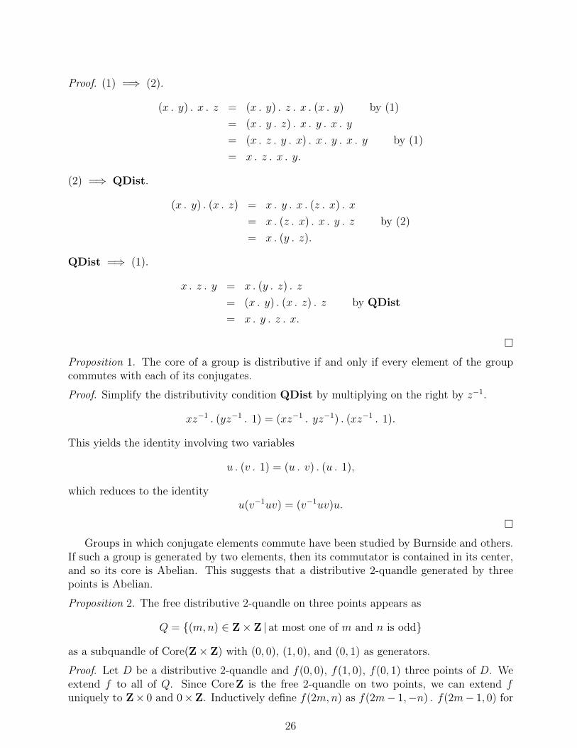
Proposition 2. The free distributive 2-quandle on three points appears as

Q = (m,n) ∈ Z× Z | at most one of m and n is odd

as a subquandle of Core(Z× Z) with (0, 0), (1, 0), and (0, 1) as generators.

Proof. Let D be a distributive 2-quandle and f(0, 0), f(1, 0), f(0, 1) three points of D. Weextend f to all of Q. Since Core Z is the free 2-quandle on two points, we can extend funiquely to Z× 0 and 0×Z. Inductively define f(2m,n) as f(2m− 1,−n) . f(2m− 1, 0) for

26

positive integers m, and f(2m,n) as f(2m + 2,−n) . f(2m + 1, 0) for negative integers m.For n = 0 this agrees with the previous definition of f(2m, 0). We show

(1) f(2m,n) . f(p, 0) = f(2p− 2m,−n)

by induction on d = |2m − p|. (1) holds for d = 0. It suffices to prove (1) for 2m > p bysymmetry at f(p, 0). (1) holds for d = 1 by definition of f(2p− 2m,−n). Assume (1) holdsfor d− 1 and d− 2. Then

f(2m,n) . f(p, 0) = f(2m− 2,−n) . f(2m− 1, 0) . f(p, 0)

= (f(2m− 2,−n) . f(p, 0)) .(f(2m− 1, 0) . f(p, 0))

= f(2p− 2m+ 2, n) . f(2p− 2m+ 1, 0)

= f(2p− 2m,−n).

Analogously, we may define f ′(m, 2n) where f ′(0, q) = f(0, q) and f ′(p, 0) = f(p, 0) so that

(1′) f ′(m, 2n) . f ′(0, q) = f ′(−m, 2q − 2n).

From distributivity, we have the identity of lemma 1,

x . z . x . y = x . y . x . z.

Taking x = f(0, 0), z = f(0, n), and y = f(m, 0), we find that f ′(2m, 2n) = f(2m, 2n). Thus,we may eliminate the primes. We have defined f on all of Q. It remains to show that f is ahomomorphism. We will show

(2) f(2m,n) . f(0, q) = f(−2m, 2q − n).

Now, (2) holds for q = 0, and by reflection through (0, 0), it suffices to show (2) for q > 0.Assume for a moment that (2) holds for q = 1. Then by induction on q > 1, we have

f(2m,n) . f(0, q) = f(2m,n) .(f(0, q − 2) . f(0, q − 1))

= f(2m,n) . f(0, q − 1) . f(0, q − 2) . f(0, q − 1)

= f(−2m, 2q − n).

Thus, it suffices to show (2) for q = 1:

(3) f(2m,n) . f(0, 1) = f(−2m, 2− n).

By a similar induction it suffices to show (3) holds for n = 0 and n = 1. The n = 0 case is aspecial case of (1′), and the n = 1 case follows from projecting f(m, 0), f(0, 0), and f(−m, 0)from f(0,−1). Thus, (2) holds. Similarly, we have

(2′) f(m, 2n) . f(p, 0) = f(2p−m,−2n)).

Finally, we show for (x, y) in Q that

(4) f(x, y) . f(2p, q) = f(4p− x, 2q − y)).

f(x, y) . f(2p, q) = f(x, y) .(f(0,−q) . f(p, 0))

= f(x, y) . f(p, 0) . f(0,−q) . f(p, 0)

= f(2p− x,−y) . f(0,−q) . f(p, 0)

= f(x− 2p, y − 2q) . f(p, 0)

= f(4p− x, 2q − y).

27

Along with (4′) we have shown that f is a homomorphism.

As a corollary, we have that any distributive 2-quandle generated by three points isAbelian.

Soublin [15] constructs a nonAbelian distributive quandle M81 of order 81. It is thesmallest nonAbelian distributive quandle satisfying x . y = y . x.

3.5 Involutions

A natural occurrence of involutory quandles is that of the set of involutions in a group G.More generally, for n a positive integer

Qn(G) = x ∈ G |xn = 1

is an n-quandle with conjugation as the quandle operation. Qn is a functor: (groups) →(n-quandles). Adjoint to Qn is the functor AdQn : (n-quandles) → (groups). For an n-quandle Q, AdQn(Q) is a group presented as

AdQn(Q) = (p, for p ∈ Q : pn = 1, p . q = q−1p q, for p, q ∈ Q).

The degree to which AdQn relates n quandles to groups may be seen in part by the followingproposition.

Proposition. For an n-quandle Q, the order of the group AdQn(Q) is no greater than n raisedto the order of Q. |AdQn(Q)| ≤ n|Q|.

Lemma. Let the elements of an n-quandle Q be well ordered. Than any element of AdQn(Q)may be written as a finite product of the generators in nondecreasing order.

Proof. The proposition follows directly from the lemma. We prove the lemma by a doubleinduction.

Let z = x1 · · ·xm be an element of G = AdQn(Q), each xi in Q, not necessarily distinct.By induction on m, the length of the product, we may assume that a product of lengthless than m may be written with the xi’s in nondecreasing order. So we may assume x1 x2 · · · xm−1. By transfinite induction on xm, we may assume that products of length mwhose first m− 1 terms are in order and whose n-th term is less than xm may be written innondecreasing order. We show now that z may be rewritten in order without increasing itslength. If xm−1 xm, then Z is already in order.

Otherwise, xm−1 xm. Let y = xm .-1 xm−1. Then xm−1xm = y xm−1, and so z =

x1 · · · xn−2y xn−1. By the first induction we may write x1 · · ·xn−2y in nondecreasing order asy1 · · · yn−1, so z = y1 · · · yn−1xn−1. By the second induction, using the fact that xn−1 ≺ xn,we may write z in nondecreasing order.

The bound of 2|Q| is achieved for finite 2-quandles satisfying x . y = x. Since AdQn(Q)maps onto InnQ, we have as a corollary that | InnQ| ≤ n|Q|.

3.6 Moufang loop cores

The functor Core : (groups) → (2-quandles) may be extended from groups to Moufangloops. Recall that a loop is a set G equipped with a binary operation (usually written

28

multiplicatively) with an identity element 1, x1 = 1x = x, such that for all a, b in G there areunique solutions to the equations xa = b and ay = b. Thus, a loop is a quasigroup with anidentity element. A loop has the inverse property when it has an operation x 7→ x−1 satisfying(xy−1)y = x and y(y−1x) = x. Such loops also satisfy x−1x = xx−1 = 1, (x−1)−1 = x,(xy)−1 = y−1x−1, and x−1(xy) = y = (yx)x−1.

A loop is a Moufang loop if it satisfies

(1) (xy)(zx) = (x(yz))x.

Moufang loops have the inverse property, and they satisfy the identities

(2) ((xy)z)y = x(y(zy)), and

(3) x(y(xz)) = ((xy)x)z.

Although a Moufang loop need not be a group, for it need not be associative, any subloopgenerated by two elements is a group. Also, if x, y, z are three elements of a Moufang loopwhich associate, that is, (xy)z = x(yz), then the subloop which they generate is a group.

For a discussion of Moufang loops and proofs of the above statements see chapter vii ofBruck’s book [3].

A basic problem of Moufang loops (and of loops and quasigroups in general) is to determinewhen two loops are isotopic. An isotopy of two quasigroups G,H consists of three bijectionsf, g, h : G→ H such that for all x, y in G

f(x)g(y) = h(xy).

Bruck defined the core of a Moufang loop as the underlying set of the loop along with thebinary operation (x, y) 7→ yx−1y (which we denote x . y) in order to have a property ofMoufang loops invariant under isotopy. If two Moufang loops are isotopic, then their coresare isomorphic. Work on cores of loops more inclusive than Moufang loops may be found inRobinson [12] and Burn [4].

Proposition 1. The core of a Moufang loop is a 2-quandle.

Proof. Axioms Q1 and QInv hold since they only involve two variables, and they hold inthe case of a group. To show axiom Q3 first observe that xz . yz = (x . y)z. Indeed,

xz . yz = (yz)(xz)−1(yz)

= (yz)(z−1x−1)(yz)

= ((yz)z−1)(x−1(yz)) by (1)

= y(x−1(yz))

= (yx−1y)z by (3)

= (x . y)z.

Similarly, zx . zy = z(x . y). Also (x . y)−1 = x−1 . y−1. Hence,

(x . z) .(y . z) = (zx−1z) .(zy−1z)

= z(x−1 . y−1)z

= z(x . y)−1z

= (x . y) . z

29

A Moufang loop is commutative if xy = yx. We will write commutative Moufang loopsadditively. We have from (2) the identity

((x+ y) + z) + y = x+ (y + (z + y)),

which is equivalent to

(4) (x+ y) + z = ((2z + z) + x)− y.Proposition 2. The core of a commutative Moufang loop is distributive.

Proof. x . y = 2y − x. 2(x . y) = 2x . 2y.

(x . y) .(w . z) = (2y − x) .(2z − x)

= (2y . 2z)− x= 2(y . z)− x= x .(y . z)

Proposition 3. The core of a Moufang loop is distributive if and only if every element com-mutes with each of its conjugates.

Proof. The proof is identical to that of proposition 1 in section 3.4.

Proposition 4. The core of a commutative Moufang loop G is Abelian if and only if G is agroup.

Proof. The proof that the core of an Abelian group is an Abelian quandle is direct.Let G be a commutative Moufang loop with an Abelian core. Abelianness gives

(4z − 2y)− (2x− w) = (4z − 2x)− (2y − w).

Setting z = 0 and negating x and y, we find

(w + 2x) + 2y = (w + 2y + 2x).

Since the subloop generated by w, 2x and 2y is associative, w, 2x, and 2y associate in anyorder. Note

(w + x) + 2y = ((2x+ 2y) + w)− x by (4)

= ((2y + w) + 2x)− x= (2y + w) + x.

Hence, w, x, and 2y associate. Finally,

(w + y) + x = ((2y + x) + w)− y by (4)

= ((x+ w) + 2y)− y= (x+ w) + y.

Thus, G is associative.

30

3.7 Distributive 2-quandles with midpoints

Definition. Let Q be a 2-quandle. A midpoint between two points x and y of Q is a point msuch that x .m = y (and so y .m = x). Q is said to have midpoints if there is a midpointbetween any two of its points.

If Q is a finite 2-quandle with midpoints, then midpoints are unique. Midpoints need notbe unique in the infinite case. Consider, for example, Q = Core R/Z. Between 0 and 1

2lie

the midpoints 14

and 34.

The assumption that a commutative Moufang loop is 2-divisible, that is, for each elementx there exists an element y such that 2y = x, implies that its core has midpoints.

Proposition. Let Q be a distributive 2-quandle with midpoints and 0 be a fixed element ofQ. Then Q has the structure of a 2-divisible commutative Moufang loop, L(Q), by takingx+ y = 0 .m where m is any midpoint between x and y.

Lemma. Let Q be a distributive 2-quandle with midpoints. Let x, y ∈ Q. Then any twomidpoints between x and y are behaviorally equivalent.

Proof of lemma. Let m be a midpoint between x and y. Let z be a point of Q. We showthat z .m depends only on z, x, and y, not on m. Take n to be a midpoint between z andy. Using a variant of the identity (1) in lemma 1, section 3.4, we have

z .m = z . n .m. z . n

= y .m. z . n

= x . z . n.

The last expression does not depend on m.

Proof of proposition. Addition is well-defined by the lemma. Clearly, addition is commutative,and 0 is an additive identity. To show that L(Q) is a loop, we must show that for all x, y ∈ Q,there is a unique z in Q such that x+ z = y. Let m be a midpoint between 0 and y, and setz = x .m. Then x+ z = y. Conversely, if x+ z = y, and m is a midpoint between x and z,then m is a midpoint between 0 and y, and by the lemma, z = x .m

Next we show the Moufang identity for commutative loops:

(x+ y) + (x+ z) = x+ (x+ (y + z)).

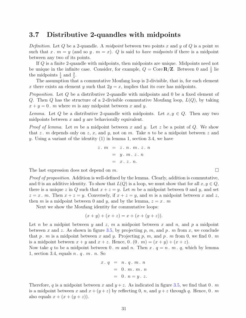
Let n be a midpint between y and z, m a midpoint between x and n, and p a midpointbetween x and z. As shown in figure 3.5, by projecting p, m, and p .m from x, we concludethat p .m is a midpoint between x and y. Projecting p, m, and p .m from 0, we find 0 .mis a midpoint between x+ y and x+ z. Hence, 0 .(0 .m) = (x+ y) + (x+ z).Now take q to be a midpoint between 0 .m and n. Then x . q = n .m. q, which by lemma1, section 3.4, equals n . q .m.n. So

x . q = n . q .m.n

= 0 .m.m.n

= 0 . n = y . z.

Therefore, q is a midpoint between x and y+ z. As indicated in figure 3.5, we find that 0 .mis a midpoint between x and x+ (y+ z) by reflecting 0, n, and y+ z through q. Hence, 0 .malso equals x+ (x+ (y + z)).

31

Figure 3.5: Midpoints

rx

r0

rp .m rm rp

rx+ y r0 .m rx+ z

ry rn rz

,,,,,,,,,,,,

AAAAAAAAAAAAAAAA

rx

r0

rn rq

r 0 .m

ry + z rx+ (y + z)

,,,,,,,,,,,,

PPPPPP

Thus, L(Q) is a Moufang loop. Finally, L(Q) is 2-divisible, since if m is a midpointbetween 0 and x, then x = 2m.

The functors Core and L are inverse to each other, so we have an isomorphism of cate-gories; the category of 2-divisible commutative Moufang loops is isomorphic to the categoryof pointed distributive 2-quandles with midpoints. By proposition 4 of section 3.6, this iso-morphism restricts to an isomorphism from the category of 2-divisible Abelian groups to thecategory of pointed Abelian 2-quandles with midpoints.

32

Chapter 4

Algebraic topology and knots

4.1 The fundamental quandle of a pair of spaces.

Consider the category P ′ of pairs of topological spaces (X,K), K a subspace of X, wherea map f : (X,K) → (Y, L) in P ′ is given by a continuous map f : X → Y such thatf−1(L) = K. Two maps f, g : (X,K)→ (Y, L) in P ′ are said to be homotopic, written f ∼ g,if there is a map h : (X × I,K × I) → (Y, L) in P ′, where I is the unit interval, such thath(x, 0) = f(x) and h(x, 1) = g(x) for all x in X. This concept of homotopy in P ′ yields acategory [P ′] of pairs of topological spaces where the maps are homotopy classes of maps inP ′.

For our purposes we must consider pointed spaces. Let P be the category whose objectsare pairs of spaces (X,K) along with a distinguished point ∗ in X −K, called the basepoint,and whose maps between pairs preserve the basepoint. If (X,K) is such a pointed pair, letX ∧ I be the quotient (X × I)/(∗ × I) of X × I. Two maps f, g : (X,K) → (Y, L) in Pare homotopic, written f ∼ g, if there is a map h : (X ∧ I,K × I) → (Y, L) in P such thath(x, 0) = f(x) and h(x, 1) = g(x) for all x in X. Let [P ] be the resulting homotopy categoryfor P .

One object of [P ] is the circle S = (S1,∅) where S1 is the unit circle in the complexplane with the basepoint at 1. S is a cogroup in [P ], that is, S has a group structure in[Pop]. Since we will be dealing with this cogroup in some detail, let us describe this structureexplicitly. We need a comultiplication µ : S → S ∨ S, a coinversion σ : S → S, and acoidentity S → (1,∅). There is only one map S → (1,∅) so it is the coidentity. Define σ byσ(z) = z−1. Represent S ∨ S as S × 1, 2 with the points (1, 1) and (1, 2) identified. Thendefine µ by

µ(eit) =

(e2it, 1) for 0 ≤ t ≤ π(e2it, 2) for π ≤ t ≤ 2π.

With these definitions S becomes a cogroup. The homotopy classes of maps from S to anyobject (X,K) form a group π(X,K) which is just the fundamental group of X−K, π1(X−K).

A map α : S → (X,K) is called a loop in X − K. If α and β are two loops, we letα−1 = σα and αβ = µ(α ∨ β). Then αα−1 ∼ 1 and (αβ)γ ∼ α(βγ).

Unfortunately, π(X,K) gives only partial information about the way that K is situatedin X, no more than the circumstantial information concerning X−K. For instance, when Kis a knot in 3-space X, π(X,K) is the knot group, and although the knot group distinguishes

33

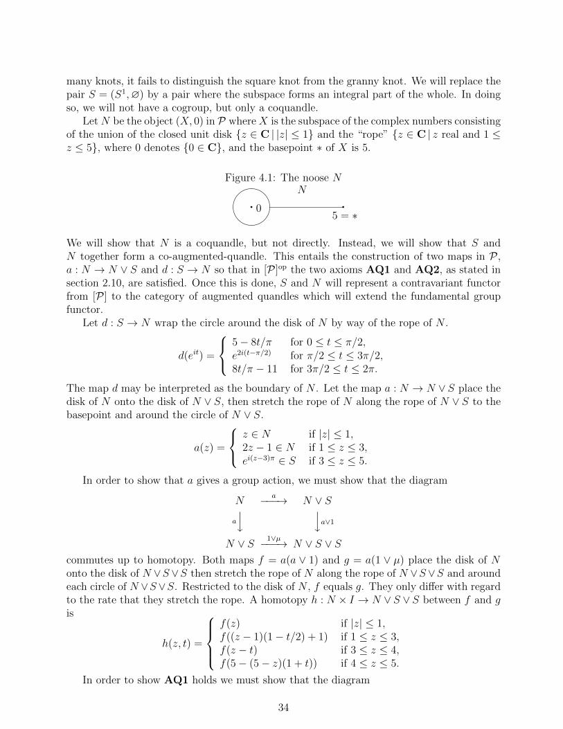
many knots, it fails to distinguish the square knot from the granny knot. We will replace thepair S = (S1,∅) by a pair where the subspace forms an integral part of the whole. In doingso, we will not have a cogroup, but only a coquandle.

Let N be the object (X, 0) in P where X is the subspace of the complex numbers consistingof the union of the closed unit disk z ∈ C | |z| ≤ 1 and the “rope” z ∈ C | z real and 1 ≤z ≤ 5, where 0 denotes 0 ∈ C, and the basepoint ∗ of X is 5.

Figure 4.1: The noose N

&%'$q 0 q

5 = ∗

N

We will show that N is a coquandle, but not directly. Instead, we will show that S andN together form a co-augmented-quandle. This entails the construction of two maps in P ,a : N → N ∨ S and d : S → N so that in [P ]op the two axioms AQ1 and AQ2, as stated insection 2.10, are satisfied. Once this is done, S and N will represent a contravariant functorfrom [P ] to the category of augmented quandles which will extend the fundamental groupfunctor.

Let d : S → N wrap the circle around the disk of N by way of the rope of N .

d(eit) =

5− 8t/π for 0 ≤ t ≤ π/2,e2i(t−π/2) for π/2 ≤ t ≤ 3π/2,8t/π − 11 for 3π/2 ≤ t ≤ 2π.

The map d may be interpreted as the boundary of N . Let the map a : N → N ∨ S place thedisk of N onto the disk of N ∨ S, then stretch the rope of N along the rope of N ∨ S to thebasepoint and around the circle of N ∨ S.

a(z) =

z ∈ N if |z| ≤ 1,2z − 1 ∈ N if 1 ≤ z ≤ 3,ei(z−3)π ∈ S if 3 ≤ z ≤ 5.

In order to show that a gives a group action, we must show that the diagram

Na−−−→ N ∨ S

a

y ya∨1N ∨ S 1∨µ−−−→ N ∨ S ∨ S

commutes up to homotopy. Both maps f = a(a ∨ 1) and g = a(1 ∨ µ) place the disk of Nonto the disk of N ∨S∨S then stretch the rope of N along the rope of N ∨S∨S and aroundeach circle of N ∨S∨S. Restricted to the disk of N , f equals g. They only differ with regardto the rate that they stretch the rope. A homotopy h : N × I → N ∨ S ∨ S between f and gis

h(z, t) =

f(z) if |z| ≤ 1,f((z − 1)(1− t/2) + 1) if 1 ≤ z ≤ 3,f(z − t) if 3 ≤ z ≤ 4,f(5− (5− z)(1 + t)) if 4 ≤ z ≤ 5.

In order to show AQ1 holds we must show that the diagram

34

Na−→ N ∨ S 1∨d−→ N ∨N

↓δN

PPPPPPPPPq1

commutes up to homotopy. Represent N ∨N as N ×1, 2 with basepoints identified. Thenthe map δ : N ∨ N → N is given by δ(z, n) = z. Let f = a(1 ∨ d)δ. Then f : N → N isformulated as

f(z) =

z if |z| ≤ 1,2(z − 1) + 1 if 1 ≤ z ≤ 3,5− 8(z − 3) if 3 ≤ z ≤ 3.5exp(2i(z − 3.5)π) if 3.5 ≤ z ≤ 4.58(z − 4.5) + 1 if 4.5 ≤ z ≤ 5.

Verbally described, f places the disk of N onto itself, then stretches the rope along andback itself, around the disk, and back to the basepoint. In the category P a homotopy isnot allowed to pass any point of X − A through A; in particular, the rope of N may notpass through the origin. The required homotopy, f ∼ 1, may be made by rotating the diskcounterclockwise one revolution while contracting the string to its initial position. Figure 4.2illustrates such a homotopy.

Figure 4.2: f = a(1 ∨ d)δ : N → N is homotopic to 1

t = 1(1) &%

'$q- ∗

t = 5/6 &%'$q

∗

t = 2/3 &%'$qAK ∗

t = 1/2 &%'$q- ∗

t = 1/4 &%'$q- ∗

t = 0(f) &%

'$q- ∗

In order to show the axiom AQ2 holds, we must verify that the diagram

35

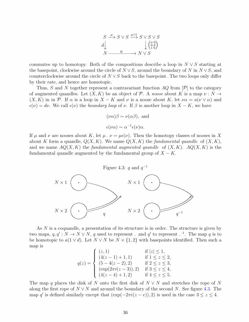
Sµ−→ S ∨ S µ∨1−→ S ∨ S ∨ S

↓dN

↓(σ 00 d1 0

)a → N ∨ S

commutes up to homotopy. Both of the compositions describe a loop in N ∨ S starting atthe basepoint, clockwise around the circle of N ∨S, around the boundary of N in N ∨S, andcounterclockwise around the circle of N ∨S back to the basepoint. The two loops only differby their rate, and hence are homotopic.

Thus, S and N together represent a contravariant function AQ from [P ] to the categoryof augmented quandles. Let (X,K) be an object of P . A noose about K is a map ν : N →(X,K) in in P . If α is a loop in X −K and ν is a noose about K, let να = a(ν ∨ α) andε(ν) = dν. We call ε(ν) the boundary loop of ν. If β is another loop in X −K, we have

(να)β ∼ ν(αβ), and

ε(να) ∼ α−1ε(ν)α.

If µ and ν are nooses about K, let µ . ν = µε(ν). Then the homotopy classes of nooses in Xabout K form a quandle, Q(X,K). We name Q(X,K) the fundamental quandle of (X,K),and we name AQ(X,K) the fundamental augmented quandle of (X,K). AQ(X,K) is thefundamental quandle augmented by the fundamental group of X −K.

Figure 4.3: q and q−1

qN × 2 q

N × 1 q∗

q−1N × 2 q

N × 1 q∗

As N is a coquandle, a presentation of its structure is in order. The structure is given bytwo maps, q, q′ : N → N ∨N , q used to represent . and q′ to represent .-1. The map q is tobe homotopic to a(1 ∨ d). Let N ∨N be N × 1, 2 with basepoints identified. Then such amap is

q(z) =

(z, 1) if |z| ≤ 1,(4(z − 1) + 1, 1) if 1 ≤ z ≤ 2,(5− 4(z − 2), 2) if 2 ≤ z ≤ 3,(exp(2πi(z − 3)), 2) if 3 ≤ z ≤ 4,(4(z − 4) + 1, 2) if 4 ≤ z ≤ 5.

The map q places the disk of N onto the first disk of N ∨ N and stretches the rope of Nalong the first rope of N ∨N and around the boundary of the second N . See figure 4.3. Themap q′ is defined similarly except that (exp(−2πi(z − e)), 2) is used in the case 3 ≤ z ≤ 4.

36

In forthcoming proofs we will have occasion to compose nooses with paths as well as loops.If ν is a noose in X about K with basepoint ∗, and α is a path in X−K from ∗ to ∗′, then letνα denote the composition. να is a noose in X about K with basepoint ∗′. Let Disk ν denotethe noose with basepoint ν(1), (Disk ν : N → (X,K) is constantly ν(1) on the rope of N).Let Rope ν denote the path from ν(1) to ∗ along the image of ν. Then ν ∼ (Disk ν)(Rope ν).

4.2 The fundamental quandle of a disk

Let (D, 0) be the object in P where D is the closed unit disk in the complex plane and 0 isthe center of the disk.

Proposition. Any element of Q(D, 0) is uniquely representable as a noose f : N → (D, 0)

f(z) =

reinθ if |z| ≤ 1, z = reiθ,1 if 1 ≤ z ≤ 5,

for a unique integer n. n is the winding number of the boundary of f around 0.

Proof. In order to simplify computations, we may take N to be (D, 0) as they are homotopi-cally equivalent in the category P . To further simplify the description of the homotopies, wewill take D to be S1 × [0,∞) union a point at infinity (to correspond to the center of D).

Let f : D → D be continuous such that f−1(∞) =∞. First we construct a homotopy sothat we may assume f(S1 × 0) ⊆ S1 × 0. Since f(S1 × 0) is compact and misses ∞, there isan x0 such that f(S1×0) ⊆ S1× [0, xo]. We use a homotopy to squeeze S1× [0, x0] to S1×0.Using the notation f(θ, x) = (f 1(θ, x), f 2(θ, x)), define h : D × I → D by

h(θ, x, t) =

(f 1(θ, x), f 2(θ, x)− tx0) if x ≥ tx0(f 1(θ, x), 0) if x ≤ tx0.

Then h(θ, x, 0) = f(θ, x) while h(θ, 0, 1) ⊆ S1×0. We may therefore assume that f(S1×0) ⊆S1 × 0.

Now f restricted to S1×0 gives a loop in S1×0, so is homotopic to the map (θ, 0)→ (nθ, 0),where n is the winding number. Then there is a map h : S1 × 0 × I → S1 × 0 such thath(θ, 0, 0) = f(θ, 0) and h(θ, 0, 1) = (nθ, 0). We construct a homotopy H : D × I → Dextending h. Let

H(θ, x, t) =

f(θ, x− t) if x ≥ t,h(θ, 0, t− x) if x ≤ t.

Then H(θ, x, 0) = f(θ, x) while H(θ, 0, 1) = (nθ, 0). Thus, we may assume f(θ, 0) = (nθ, 0).Finally, we show f is homotopic to the map (θ, x) 7→ (nθ, x). We will define a homotopy

H : D × I → D which spreads the influence of the restriction of f to S1 × 0 down the entirecylinder S1 × [0,∞). Let

H(θ, x, t) = (f 1(θ, (1− t)x), f 2(1− t)x+ tx).

Then H(θ, x, 0) = (f 1(θ, x), f 2(θ, x)) = f(θ, x), and H(θ, x, 1) = (f 1(θ, 0), f 2(θ, 0) + x) =(nθ, x). We should check that setting H(∞, t) to ∞ leaves H continuous. Given N > 0,we must show there exists an M > 0 such that for all x > M , H2(θ, x, t) > N . Let M1 be

37

such that if x > M1, then f 2(θ, x) > N . Let M = max2M1, 2N. Suppose x > M . Thenx/2 > M1 and x/2 > N .

Case 1. t ≥ 12. H2(θ, x, t) = f 2(θ, (1− t)x) + tx ≥ tx ≥ x/2 > N .

Case 2. t ≤ 12. H2(θ, x, t) = f 2(θ, (1− t)x) + tx ≥ f 2(θ, (1− t)x) which is greater than N

since (1− t)x ≥ x/2 > M1.

Thus, H gives a homotopy of f to the map (θ, x) 7→ (nθ, x).

The quandle operation on Q(D, 0) is first projection, that is x . y = x.

4.3 The Seifert-Van Kampen theorem

Recall the Seifert-Van Kampen theorem for the fundamental group. Let X be an arcwiseconnected topological space with a basepoint, and let Ui be a covering of X by arcwiseconnected open sets closed under pairwise intersections such that each open set Ui containsthe basepoint. Then

π1(X) = lim−→ π1(Ui).

We will prove an analogous theorem for the fundamental quandle of a pair of spaces.

Theorem. Let (X,K) be an object in P . Let Ui be a covering of X closed under pairwiseintersection. Assume for each index i that Ui is a neighborhood of Ui ∩K and that Ui − k isarcwise connected and contains the basepoint of X. Then

AQ(X,K) = lim−→AQ(Ui, Ui ∩K).

Proof. Let AQ(X,K) = (Q,G). Then by the Seifert-Van Kampen theorem, G = π1(X−K) =lim−→ π1(Ui −K). By the theorem of section 2.10, the lim−→AQ(Ui, Ui ∩K) is then of the form(L,G). By the universal property of (L,G), there is a unique ψ : L→ Q determined by themaps AQ(Ui, Ui ∩K)→ AQ(X,K) = (Q,G). We will show ψ is an isomorphism.

Surjectivity of ψ. By the theorem of section 2.10, it suffices to show that every noose γabout K is homotopic to some αβ where α is a noose in some (Ui, Ui ∩K), and β is a loopin X − K. Let γ be an arbitrary noose about K. γ(0) lies in some Ui. Since γ−1(Ui) is aneighborhood of 0 in N , there is some r > 0 such that |z| ≤ r implies γ(z) ∈ Ui. Using thehomotopy

H(z) =

γ(zr) if |z| ≤ 1γ((z − 1)(5− 4)/r + r) if 1 ≤ z ≤ 5,

we may adjust γ so that we may assume γ(z) ∈ Ui for |z| ≤ 1. Choose a path δ in Ui −Kfrom γ(1) to ∗. Let α be the noose (Disk γ)δ in (Ui, Ui ∩K) and β be the loop δ−1(Rope γ)in X −K. Then αβ = (Disk γ)δδ−1(Rope γ) ∼ (Disk γ)(Rope γ) ∼ γ as required.

Injectivity of ψ. It suffices to show that if αβ ∼ α′β′ where α is a noose in (Ui, Ui ∩K),β and β′ are loops in X − K, and α′ is a noose in (Ui′ , Ui′ ∩ K), then as elements of L,αβ = α′β′. Let H effect the homotopy αβ ∼ α′β′; H : N × I → X, H(z, 0) = (αβ)(z),H(z, 1) = (α′β′)(z). The inverse images of the open sets Ui under H(0, t) cover the unitinterval I. Hence, we may divide I into subintervals 0 = t0 < t1 < · · · < tn = 1 so that foreach j = 1, . . . , n there is an index i(j) for which H(0, t) ∈ Ui(j) when ti−1 ≤ t ≤ ti. We maytake i(1) = i and i(n) = i′. There is an r > 0 so that for |z| ≤ r and tj−1 ≤ t ≤ tj we have

38

H(z, t) ∈ Ui(j). One r suffices for all j. By appropriate adjustments of α, α′, and H we mayassume r = 1.

Figure 4.4 illustrates the remainder of the proof. For j = 0, 1, . . . , n define the noosesγj = H(z, tj) in (X,K). Also choose paths δj from γj(1) to ∗ in Ui(j−1) ∩ Ui(j) − K forj = 1, 2, . . . , n− 1, and set δ0 = Ropeα and δn = Ropeα′.

Figure 4.4: Seifert-Van Kampen noose homotopy

I0= t0 t1 t2 tn =1

0

q q q q1

ε1 ε2

5γ0∗

∗

β=β0

α=α0

γ1∗γ2∗

γn∗

∗

β′=βn

α′=αn

δ0 δ1

∗

δ2

∗

δn

For j = 0, . . . , n define αj to be the noose (Disk γj)δj in (Ui(j−1)∩Ui(j)−K,Ui(j−1)∩Ui(j))and βj to be the loop δ−1j (Rope γj) in X−K. Then α = α0, α

′ = αn. As nooses in (Ui, Ui∩K)and (Ui′ , Ui′ ∩K), αβ ∼ α0β0 and α′β′ ∼ αnβn, respectively. In order to show αβ equals α′β′

in L, we will show for j = 1, . . . , n that αj−1βj−1 equals αjβj.Fix j between 1 and n. We must show αj−1 = αjβjβ

−1j−1. Let εj be the path from γj−1(1)

to γj(1) in Ui(j−1)−K given by εj(t) = H(1, tj−1 + t(tj− tj−1)). The portion of the homotopyH on [1, 5]× [tj−1, tj] yields a homotopy in X −K of εj to (Rope γj−1)(Rope γj)

−1. Thus

βj−1β−1j = δ−1j−1(Rope γj−1)(Rope γj)

−1δj

= δ−1j−1εjδj

as elements of π1(X−K). The noose αjδ−1j−1εjδj lies entirely in Ui(j−1) as does αj−1. Moreover,

the restriction of H to |z| ≤ 1 × [tj−1, tj] has an image in Ui(j−1) and yields a homotopy ofαj−1 to αjδ

−1j−1εjδj in (Ui(j−1) ∩K,Ui(j−1)). Thus, αj−1 = αjδ

−1j−1εjδj = αjβj−1β

−1j as elements

of L.

Corollary. Let (X,K) be an object in P . Let U and V be an open covering of X such thatU −K, V −K, and U ∩ V −K are arcwise connected and contain the basepoint of X. Then

39

AQ(X,K) is the pushout

AQ(U ∩ V, U ∩ V ∩K) −−−→ AQ(V, V ∩K)y yAQ(U,U ∩K) −−−→ AQ(X,K)

4.4 Applications of the Seifert-Van Kampen theorem

The proposition in section 4.2 implies that if K is a point in the plane X, then AQ(X,K) =(ConjF, F ) where F is the free group on one element. Consider a generalization where X isa 2-manifold.

Proposition 1. Let K be a point in a 2-manifold X, and let G = π1(X −K). Let U be theunion of a small disk around K and a path to the basepoint, and let α be a loop in U windingonce around K. Let F be the free group generated by one element and f : F → G send thegenerator of F to the homotopy class of α. Then

AQ(K,X) = (ConjF ⊗F G,G).

Proof. Let V = X −K. Then by the Seifert-Van Kampen theorem,

AQ(U ∩ V,∅) = (∅, F ) −−−→ AQ(V,∅) = (∅, G)y yAQ(U,K) = (ConjF, F ) −−−→ AQ(X,K)

is a pushout square. Hence, by the theorem of section 2.10, we have AQ(K,X) = (ConjF ⊗FG,G).

Another generalization of the same proposition is where X remains the plane and K is adiscrete subset of X. For each point k in K let α(k) be a small loop winding once around k.Then G = π1(X −K) is free on α(k) | k ∈ K. For k in K let Fk be the free group on α(k)and Fk → G the inclusion homomorphism.

Proposition 2. X, K, G, Fk as above. Then

AQ(X,K) = (⋃k∈K

ConjFk ⊗FkG,G).

Proof. For k in K let Uk = (X − K) ∪ k. Then AQ(Uk, k) = (ConjFa ⊗Fa G,G) byproposition 1. If k, l ∈ K, k 6= l, then AQ(Uk ∩Ul,∅) = (∅, G). Thus, AQ(X,K) is the limitof the diagram

40

(∅, G)

*

(ConjFk ⊗FkG,G)

:

...XXXXXXXXzHHH

HHHHHj (ConjFl ⊗Fl

G,G)

which is (⋃k∈K ConjFk ⊗Fk

G,G).

In most of the applications that follow K will be a submanifold of X of codimension two.When this is the case we will try to restrict our attention to those nooses in X “windingonce” about K. For instance if X is an oriented 2-manifold and K is a discrete subset of X,“winding once” is well-defined.

Let X be the plane and K a discrete subset of X. Orient X and let Q consist of the nooseswhich wind exactly once (in the positive sense) around a point of K, and let AQ(X,K) be Qaugmented by G = π1(X−K). Then by proposition 2, AQ(X,K) = (

⋃k∈Kα(k)⊗Fk

G,G).

Then Q is just the free quandle on |K| elements, and is isomorphic to the quandle consistingof the conjugates of the generators of G.

4.5 Knot quandles

Recall that a knot is a subspace K of the 3-sphere X = S3 which is homeomorphic to acircle. A link is a subspace K of X homeomorphic to a disjoint union of circles. Two knotsor links K and K ′ are equivalent if there is a homeomorphism h of X such that h(K) = K ′,that is, in the category P , (X,K) is homeomorphic to (X,K ′). We will deal with orientedspaces; we assume X and K are endowed with orientations. (If K is a link, then we assumeeach component circle is oriented.) An oriented equivalence of K and K ′ is an orientation-preserving homeomorphism h of X such that h(K) = K ′ and h preserves the orientationof each component of K. An equivalence class of oriented knots or links (under orientedequivalence) is called an oriented knot type or oriented link type, respectively. We assume allknots, links, and equivalences are oriented and henceforth omit the adjective “oriented”.

The fundamental group of X − K, π1(X − K), is called the knot group (or link group).This definition assumes either that X −K has a designated basepoint or else that the knotgroup is only defined up to noncanonical isomorphism; we assume a basepoint.

Recall that a tame knot is a knot equivalent to a closed polygonal curve in X. Some ofthe results below are restricted to tame knots and tame links.

Associated to a knot (X,K) we have the fundamental quandle Q(X,K). An element ofQ(X,K) is represented by a noose ν about K. The boundary loop ε(ν) may or may not linkwith K as shown in figure 4.5.In order to decide when a loop in X −K links once with K, it suffices to choose a generatorof H1(X −K) ∼= Z. Then loops homologous to that generator have linking number 1 withK. Since we assume K and X have orientations, such a generator may be naturally chosen(say, by the right-hand rule).

41

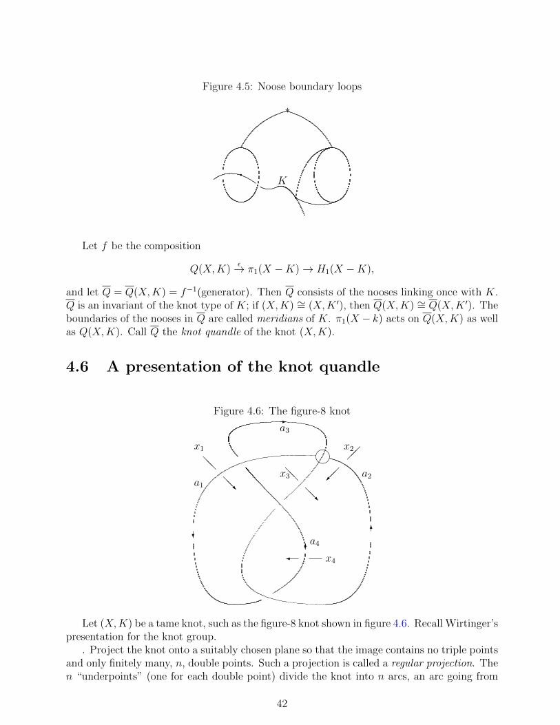
Figure 4.5: Noose boundary loops

∗

Kq

q

Let f be the composition

Q(X,K)ε→ π1(X −K)→ H1(X −K),

and let Q = Q(X,K) = f−1(generator). Then Q consists of the nooses linking once with K.Q is an invariant of the knot type of K; if (X,K) ∼= (X,K ′), then Q(X,K) ∼= Q(X,K ′). Theboundaries of the nooses in Q are called meridians of K. π1(X − k) acts on Q(X,K) as wellas Q(X,K). Call Q the knot quandle of the knot (X,K).

4.6 A presentation of the knot quandle

Figure 4.6: The figure-8 knot

6

-

6?

@@

x1

@@R

x2

@@x3

@@R

x4

a1a2

a3

a4

n

Let (X,K) be a tame knot, such as the figure-8 knot shown in figure 4.6. Recall Wirtinger’spresentation for the knot group.

. Project the knot onto a suitably chosen plane so that the image contains no triple pointsand only finitely many, n, double points. Such a projection is called a regular projection. Then “underpoints” (one for each double point) divide the knot into n arcs, an arc going from

42

Figure 4.7: A knot crossing

a1

a2

a3

BBx3

BBN

x1

x2

@x3

@R

one underpass, over whatever overpasses there may be, to another underpass. Label thearcs a1, a2, . . . , an, placing the labels each to the right of the knot (using the orientation of(X,K)). For each arc ai pass a loop xi in X −K under the arc ai from right to left. Theseloops generate the knot group. Each underpass yields one relation among the loops. Forinstance, the circled intersection of the knot in figure 4.6, blown up in figure 4.7, yields therelation x−13 x1x3 = x2. Together these n generators and n relations give a presentation of theknot. For the figure-8 knot we have the presentation

G = (x1, x2, x3, x4 : x−13 x1x3 = x2, x4x2x−14 = x3, x

−11 x3x1 = x4, x2x4x

−12 = x1).

Since each relation states that one generator is a conjugate of another, we may give a pre-sentation of a quandle just by using quandle notation. For the figure-8 knot we then have

Q = (x1, x2, x3, x4 : x1 . x3 = x2, x2 .-1 x4 = x3, x3 . x1 = x4, x4 .

-1 x2 = x1).

By construction, AdconjQ = G. We may arrive at the same presentation more simply. Takea regular projection of the knot. Label the arcs putting the labels always on the one side of

the knot. For each intersection derive a relation on the arcs, as a c

bgives

a . b = c, while a c

b

gives a .-1 b = c. The n relations on the n generators

give a presentation of the quandle.In section 4.7 we will give a direct combinatorial demonstration that this quandle is an

invariant of the knot (that is, it does not depend on the choice of regular projection). In4.8 we show that this quandle is isomorphic to the knot quandle defined in 4.5. In 4.9 werepresent the knot quandle in terms of the knot group and show that it is a complete knotinvariant. That is, if Q(K) ∼= Q(K ′), then K is equivalent to K ′.

43

Figure 4.8: Basic knot deformations

Ω1 - -

Ω2 -

Ω3 -

4.7 The invariance of the knot quandle

In this section we directly demonstrate the invariance of the quandle of a tame knot givenby generators and relations as described in the previous section. There are three basic defor-mations of regular projections of knots which do not change the knot type. The deformationΩ1 removes or adds a kink, Ω2 slides one arc under another, and Ω3 slides an arc under anintersection.

These three deformations account for the equivalences among tame knots in the followingsense. If two tame knots are equivalent, then for any regular projections of the two knots,there is a sequence of basic deformations transforming one projection into the other. Adetailed proof of this fact is proved by Alexander and Briggs [1]. See also Reidemeister [11].In order to show the invariance of the knot quandle it suffices to show its invariance underthese basic deformations.

Figure 4.9: Invariance under Ω1

- -

a

a .-1 a

a

a

a .-1 a

a

- -

a

a . a

a

a

a . a

a

For the deformation Ω1, we have two cases depending on which side of the arc is labelled.

44

Figure 4.9 indicates that the knot quandle is invariant under Ω1 since in a quandle, theidentities x . x = x and x .-1 x = x are satisfied.

Figure 4.10: Invariance under Ω2

-

a

a

b

b

a

a

b

b . a .-1a

-

a

a

b

b

a

a

b

b .-1a .a

Deformation Ω2 requires that x . y .-1 y = x and x .-1 y . y = x as shown in figure 4.10.

Figure 4.11: Invariance under Ω3

a

b

c a . cb . c

(a.c) .(b.c)-

a

b

c

a.b

b . c

a.b . c

a

b

c a.-1cb.-1c

(a.-1c) .(b.-1c)-

a

b

c

a.b

b.-1c

a.b.-1c

The deformation Ω3 gives four requirements depending again on the labeling. Figure 4.11illustrates two of these requirements.

The requirements for the invariance of the knot quandle under the basic deformations areall satisfied. Thus, the quandle is an invariant of the knot type.

4.8 A presentation of the knot quandle (continued)

Proposition. Let K be a tame knot and Q be the quandle presented in terms of a regularprojection as described in section 4.6. Then Q is isomorphic to the knot quandle Q definedin section 4.5.

Proof. Assume that the projection p of the knot to the plane is projection from the basepoint∗. Label the arcs in order a1, a2, . . . , an. For i = 1, . . . , n, let bi be a path down from ∗ to thecenter of the arc ai. Let γi be the loop which travels from ∗ down bi, along ai and ai+1, thenup bi+1 to ∗ as illustrated in figure 4.12.Let Ui be a small toroidal neighborhood of γi. Then Ui−1 ∩Ui is a neighborhood of bi. Let Vbe X −K. Then X = V ∪ U1 ∪ · · · ∪ Un. In order to construct Q, we need to know only thequandles of (Ui, Ui∩K), (Ui∩Ui+1, Ui∩Ui+1∩K), (V,∅), (Ui∩V,∅), and (Ui∩Ui+1∩V,∅).

45

Figure 4.12: The loop γi

bi I

bi+1

∗

r- -

ai ai+1

Let νi be a noose in Ui−1 ∩Ui linking once about ai. Then π1(Ui−1 ∩Ui−K) = (xi) is thefree group on one element xi = ε(νi). Thus

AQ(Ui−1 ∩ Ui, Ui−1 ∩ Ui ∩K) = (Conj(xi), (xi)).

Restricting to the nooses linking once with K, we have

AQ(Ui−1 ∩ Ui, Ui−1 ∩ Ui ∩K) = (xi, (xi)).

Let G = π1(X −K) and Gi = π1(Ui −K). Then

AQ(Ui, Ui ∩K) = (Conj(xi)⊗(xi) Gi, Gi), and

AQ(Ui, Ui ∩K) = (xi ⊗(xi) Gi, Gi).

In order to find AQ(X,K), we may first tensor the various AQ with G = π1(X − K).According to the theorem of section 2.10 and the Seifert-Van Kampen theorem, upon takingthe colimit of the various AQ⊗G, we will have AQ(X,K).

Both AQ(Ui−1 ∩ Ui, Ui−1 ∩ Ui ∩ K) and AQ(Ui, Ui ∩ K) become (xi ⊗(xi) G,G) whentensored with G. Thus, Q is generated by the x1, . . . , xn modulo the relations induced bytensoring with G. These relations are determined by the action of the generators of G on Qand the relations among the generators of G. It is exactly these relations which were used inthe definition of Q in section 4.6. Thus, Q ∼= Q.

We have already noted and used the fact that AdconjQ is the knot group G. As Q isisomorphic to the knot quandle Q, we have AdconjQ ∼= G. In particular, ε(Q) generates G.

Corollary. Let K be a tame knot, G its knot group, and Q its knot quandle. Then Q×G→ Qis a transitive group action.

Proof. In order to show G acts transitively on Q it suffices to show that for generators a, bof Q there is an x in G such that ax = b. But by passing under sufficiently many arcs of theregular projection, a becomes b, as suggested in the drawing

a

a1a2

· · ·

ak b

46

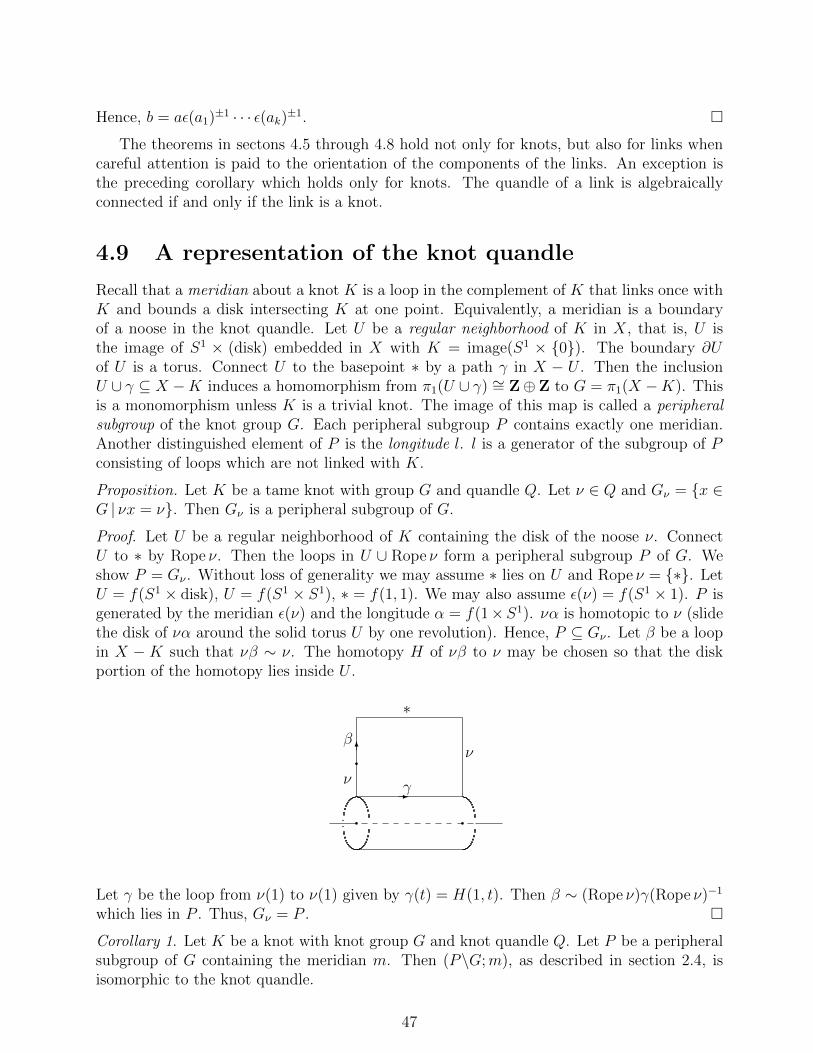
Hence, b = aε(a1)±1 · · · ε(ak)±1.

The theorems in sectons 4.5 through 4.8 hold not only for knots, but also for links whencareful attention is paid to the orientation of the components of the links. An exception isthe preceding corollary which holds only for knots. The quandle of a link is algebraicallyconnected if and only if the link is a knot.

4.9 A representation of the knot quandle

Recall that a meridian about a knot K is a loop in the complement of K that links once withK and bounds a disk intersecting K at one point. Equivalently, a meridian is a boundaryof a noose in the knot quandle. Let U be a regular neighborhood of K in X, that is, U isthe image of S1 × (disk) embedded in X with K = image(S1 × 0). The boundary ∂Uof U is a torus. Connect U to the basepoint ∗ by a path γ in X − U . Then the inclusionU ∪ γ ⊆ X −K induces a homomorphism from π1(U ∪ γ) ∼= Z⊕Z to G = π1(X −K). Thisis a monomorphism unless K is a trivial knot. The image of this map is called a peripheralsubgroup of the knot group G. Each peripheral subgroup P contains exactly one meridian.Another distinguished element of P is the longitude l. l is a generator of the subgroup of Pconsisting of loops which are not linked with K.

Proposition. Let K be a tame knot with group G and quandle Q. Let ν ∈ Q and Gν = x ∈G | νx = ν. Then Gν is a peripheral subgroup of G.

Proof. Let U be a regular neighborhood of K containing the disk of the noose ν. ConnectU to ∗ by Rope ν. Then the loops in U ∪ Rope ν form a peripheral subgroup P of G. Weshow P = Gν . Without loss of generality we may assume ∗ lies on U and Rope ν = ∗. LetU = f(S1 × disk), U = f(S1 × S1), ∗ = f(1, 1). We may also assume ε(ν) = f(S1 × 1). P isgenerated by the meridian ε(ν) and the longitude α = f(1×S1). να is homotopic to ν (slidethe disk of να around the solid torus U by one revolution). Hence, P ⊆ Gν . Let β be a loopin X − K such that νβ ∼ ν. The homotopy H of νβ to ν may be chosen so that the diskportion of the homotopy lies inside U .

∗

γ-ν

q6β ν

q q

Let γ be the loop from ν(1) to ν(1) given by γ(t) = H(1, t). Then β ∼ (Rope ν)γ(Rope ν)−1

which lies in P . Thus, Gν = P .

Corollary 1. Let K be a knot with knot group G and knot quandle Q. Let P be a peripheralsubgroup of G containing the meridian m. Then (P\G;m), as described in section 2.4, isisomorphic to the knot quandle.

47

Proof. Follows from the corollary of section 4.8.

Thus, the knot quandle contains the same information as the triple (G,P,m) consistingof the knot group G, a peripheral subgroup P , and a meridian m in P .

Neuwirth [10]] remarks that if two tame knot groups are isomorphic by a map which sendsa meridian to a meridian and the group system (the conjugate peripheral subgroups) of oneonto the group system of the other, then the (unoriented) knots are equivalent. Conway andGordon [6] use a slightly stronger principle to construct a group that classifies oriented knots.If two tame knot groups are isomorphic by a map which sends a meridian and correspondinglongitude of one onto those of the other, then the oriented knots are equivalent. A proof ofthis principle may be found in Waldhausen [19].

Corollary 2. If the knot quandles of two tame knots are isomorphic, then the (unoriented)knots are equivalent.

Other algebraic characterizations of knots have been described by Simon [14] and Whitten[20]. The constructions given by Conway and Gordon, Simon, and Whitten are not functorial,unlike the knot quandle.

4.10 The Alexander invariant of a knot

Let K be a knot in X = S3 and Y = X − K. Let Y be the infinite cyclic cover of Y .Then π1(Y ) = G′ = [G,G] where G = π1(Y ) is the knot group. Also G/G′ = Z andH1(Y ) ∼= G′/G′′. If x in G is such that the map G → G/G′ ∼= Z sends x to 1, thenconjugation by x gives an automorphism t of H1(Y ), and t is independent of x. Thus, H1(Y )is not only an Abelian group, but also a module over the ring Λ = Z[t, t−1]. This Λ-module iscalled the Alexander invariant A of the knot K. We will show in this section that A carriesthe same information as the Abelian knot quandle.

The usual presentation of the Alexander invariant is by means of a matrix. Take a Seifertsurface for the knot K and let n be the genus of the surface. Let a1, . . . , an be generatingcycles for the homology of the surface. and let vij be the linking number of ai with aj. Thematrix (vij) is called a Seifert matrix of the knot. P = (vij − tvji) is an Alexander matrix ofthe knot. The entries of P lie in Λ. Then the Alexander invariant is the cokernel

Λn P→Λn → A→ 0.

The determinant of P is called the Alexander polynomial ∆(t) of the knot. ∆(t) is definedonly up to a unit of Λ. One important property of ∆(t) is that |∆(1)| = 1. A more directdefinition of ∆(t) is that it is a generator of the annihilator ideal of A.

We first show that A may be constructed from the Abelian knot quandle AbQ. As notedin section 4.8, AdconjQ = G. Hence Adconj AbQ = G/N where N is the normal subgroupof G generated by elements of the form

ab−1ca−1bc−1, with a, b, c ∈ ε(Q).

Lemma 1. N = G′′.

Proof. Part 1. N ⊆ G′′. Let a, b, c ∈ ε(Q). Since Q is algebraically connected, there existx, y in G such that b = x−1ax and c = y−1ay. Then

ab−1ca−1bc−1 = (ax−1a−1x)(y−1aya−1)(x−1axy−1a−1y).

48

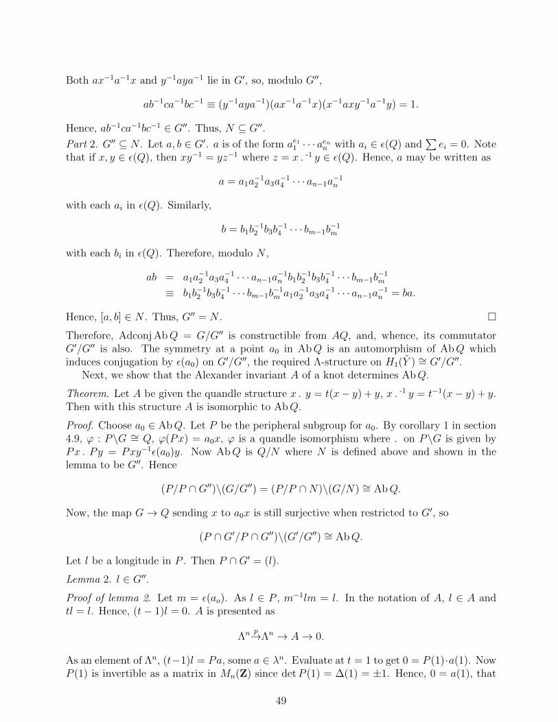
Both ax−1a−1x and y−1aya−1 lie in G′, so, modulo G′′,

ab−1ca−1bc−1 ≡ (y−1aya−1)(ax−1a−1x)(x−1axy−1a−1y) = 1.

Hence, ab−1ca−1bc−1 ∈ G′′. Thus, N ⊆ G′′.

Part 2. G′′ ⊆ N . Let a, b ∈ G′. a is of the form ae11 · · · aenn with ai ∈ ε(Q) and∑ei = 0. Note

that if x, y ∈ ε(Q), then xy−1 = yz−1 where z = x .-1 y ∈ ε(Q). Hence, a may be written as

a = a1a−12 a3a

−14 · · · an−1a−1n

with each ai in ε(Q). Similarly,

b = b1b−12 b3b

−14 · · · bm−1b−1m

with each bi in ε(Q). Therefore, modulo N ,

ab = a1a−12 a3a

−14 · · · an−1a−1n b1b

−12 b3b

−14 · · · bm−1b−1m

≡ b1b−12 b3b

−14 · · · bm−1b−1m a1a

−12 a3a

−14 · · · an−1a−1n = ba.

Hence, [a, b] ∈ N . Thus, G′′ = N .

Therefore, Adconj AbQ = G/G′′ is constructible from AQ, and, whence, its commutatorG′/G′′ is also. The symmetry at a point a0 in AbQ is an automorphism of AbQ whichinduces conjugation by ε(a0) on G′/G′′, the required Λ-structure on H1(Y ) ∼= G′/G′′.

Next, we show that the Alexander invariant A of a knot determines AbQ.

Theorem. Let A be given the quandle structure x . y = t(x− y) + y, x .-1 y = t−1(x− y) + y.Then with this structure A is isomorphic to AbQ.

Proof. Choose a0 ∈ AbQ. Let P be the peripheral subgroup for a0. By corollary 1 in section4.9, ϕ : P\G ∼= Q, ϕ(Px) = a0x, ϕ is a quandle isomorphism where . on P\G is given byPx .Py = Pxy−1ε(a0)y. Now AbQ is Q/N where N is defined above and shown in thelemma to be G′′. Hence

(P/P ∩G′′)\(G/G′′) = (P/P ∩N)\(G/N) ∼= AbQ.

Now, the map G→ Q sending x to a0x is still surjective when restricted to G′, so

(P ∩G′/P ∩G′′)\(G′/G′′) ∼= AbQ.

Let l be a longitude in P . Then P ∩G′ = (l).

Lemma 2. l ∈ G′′.Proof of lemma 2. Let m = ε(ao). As l ∈ P , m−1lm = l. In the notation of A, l ∈ A andtl = l. Hence, (t− 1)l = 0. A is presented as

Λn p→Λn → A→ 0.

As an element of Λn, (t−1)l = Pa, some a ∈ λn. Evaluate at t = 1 to get 0 = P (1)·a(1). NowP (1) is invertible as a matrix in Mn(Z) since detP (1) = ∆(1) = ±1. Hence, 0 = a(1), that

49

is, (t− 1) divides a, and a = (t− 1)b. So (t− 1) = P · (t− 1)b. Therefore, l = Pb ∈ image P .So l = 0 in A, l ∈ G′′.

Proof of theorem continued. So P ∩G′′ = (l) = P ∩G′. Therefore, G′/G′′ = AbQ. Examinethe quandle structure on G′/G′′. In P\G, . is

Px .Py = Pxy−1my = Pmxy−1my = P (x .m)(y .m)−1y.

So in G′/G′′, . isx . y = (x .m)(y .m)−1y

which in the notation of A becomes

x . y = tx− ty + y = tx+ (1− t)y.

The Alexander invariant is not enough to distinguish all knots from the trivial knot. Forinstance, the Alexander invariant of any doubled knot is trivial.

4.11 The cyclic invariants of a knot

In this section let K be a knot in X = S3 and Y the complement of the knot. Let n be apositive integer. Let Yn be the n-fold cyclic cover of Y and Σn be the n-fold branched cycliccover. Then H1(Yn) ∼= H1(Σn) ⊕ Z. H1(Σn) is a finite Abelian group. The n-th torsionnumbers of K are the subscripts in the canonical decomposition

H1(Σn) ∼= Zk1 ⊕ · · · ⊕ Zkr , ki | ki+1, i = 1, . . . , r − 1.

The order of H1(Σ2) is called the determinant of K, detK. Let P (t) = (vij − tvji) be anAlexander matrix for K. Then P (−1) = (vij + vji) presents H1(Σ2) as a module over Z. Thedeterminant of P (−1) gives detK; detK = | detP (−1)|. Hence, the Alexander polynomial∆(t) evaluated at −1 gives detK; detK = |∆(−1)|.

H1(Σn) has an automorphism induced from conjugation by an x in G = π1(Y ) for whichG→ Z sends x to 1. That is, H1(Σn) is a module over Λn = Z[t]/(tn− 1). Then H1(Σn) hasa quandle structure given by the formula x . y = tx + (1 − t)y. With this structure H1(Σn)is an n-quandle, in fact, it is the largest quotient of the Alexander invariant which is an nquandle. For n = 2, H1(Σn) is the involutory Abelian knot quandle.

4.12 The involutory knot quandle

Let K be a knot with quandle Q. The involutory knot quandle Q2 results from imposing theidentity (x . y) . y = x on Q.

Example 1. The trefoil knot 31.Q = (a, b, c : a . b = c, b . c = a, c . a = b). Q2 has the same presentation as Q as long asthe relations (x . y) . y = x are understood. Viewed with geodesics (see section 3.1), Q2 hasthree points shown to the right.

50

Figure 4.13: The trefoil knot 31

b

a

c &%'$qa qbqc

Figure 4.14: The figure-8 knot 41

a b

c

d &%'$qqc qa

qb qd

Example 2. The figure-8 knot 41.Q = (a, b, c, d : a . c = b, b .-1 d = c, c . a = d, d .-1 b = a).Q2 = (a, b, c, d : a . c = b, b . d = c, c . a = d, d . b = a).Very little work shows |Q2| = 5.

For these two examples Q2 is Abelian as well as involutory. The next example has anonAbelian Q2.

Example 3. The knot 10124.

bc

d

e

f

g

h

i

ja

Figure 4.15: The knot 10124

The Alexander polynomial of 10124 is ∆(t) = t−4 − t−3 + t−1 − 1 + t − t3 + t4, so thedeterminant of 10124 is 1. Thus, AbQ2 is trivial. A few computations will show that Q2 maybe faithfully represented as the 30 edges of a dodecahedron projected onto a sphere. Figure4.16 displays these points in stereographic projection in the plane.

51

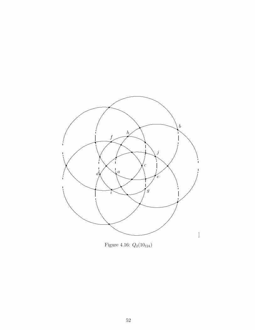
ra

rb

r crd re

rf

rg

rh

ri

rjr

r

rr

r

r

r

r

rr

r

rr

r

r

r

r

r

r

r

]

Figure 4.16: Q2(10124)

52

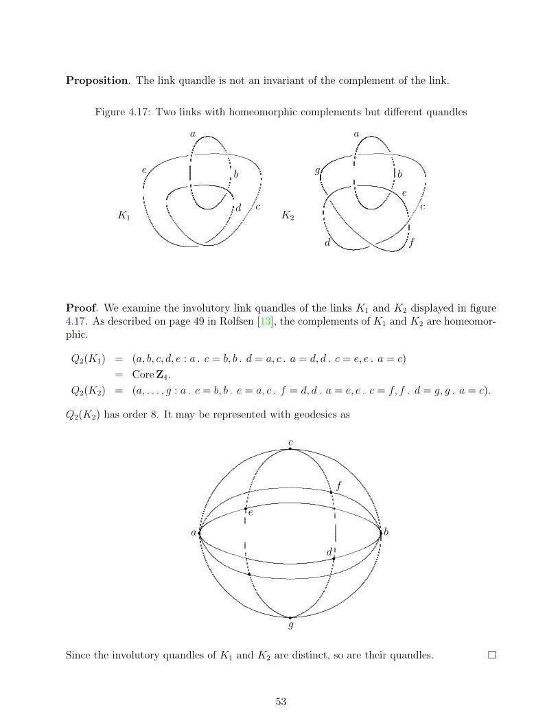
Proposition. The link quandle is not an invariant of the complement of the link.

Figure 4.17: Two links with homeomorphic complements but different quandles

K1

a

b

cd

e

K2

a

b

c

d

e

f

g

Proof. We examine the involutory link quandles of the links K1 and K2 displayed in figure4.17. As described on page 49 in Rolfsen [13], the complements of K1 and K2 are homeomor-phic.

Q2(K1) = (a, b, c, d, e : a . c = b, b . d = a, c . a = d, d . c = e, e . a = c)

= Core Z4.

Q2(K2) = (a, . . . , g : a . c = b, b . e = a, c . f = d, d . a = e, e . c = f, f . d = g, g . a = c).

Q2(K2) has order 8. It may be represented with geodesics as

ra rb

rc

rd

re

r f

rg

r

Since the involutory quandles of K1 and K2 are distinct, so are their quandles.

53

Bibliography

[1] Alexander, J. W., and G. B. Briggs, On types of knotted curves. Ann. of Math. 28(1926), 562–566.

[2] Blaschke, W., and G. Bol, Geometrie der Gewebe. Springer, Berlin, 1938.

[3] Bruck, R., H., A Survey of Binary Systems. Springer, Berlin, 1958.

[4] Burn, R. P., Finite Bol loops. Math. Proc. Cambridge Phil. Soc. 84 (1978), 377–385.

[5] Burstin, C., and W. Mayer, Distributive Gruppen, J. Reine Angew. Math. 160 (1929),111–130.

[6] Conway, J. H., and C. McA. Gordon, A group to classify knots, Bull. London Math. Soc.7 (1975), 84–88.

[7] Loos, O., Spiegelungsraume und homogene symmetrische Raume, Math. Z. 99 (1967),141–170.

[8] Loos, O., Symmetric Spaces. Benjamin, New York, 1969.

[9] Moufang, R., Zur Struktur von Alternativekorpern, Math. Ann. 110 (1935), 416–430.

[10] Neuworth, L. P., Knot Groups. Princeton Univ. Press, 1965.

[11] Reidemeister, K., Knotentheorie. Chelsea, New York, 1949 (reprint).

[12] Robinson, D. A., Bol loops, Trans. Amer. Math. Soc. 123 (1966), 341–354.

[13] Rolfsen, D., Knots and Links. Publish or Perish, Berkeley, 1976.

[14] Simon, J., An algebraic classification of knots in S3, Ann. of Math. 93 (1973), 1–13.

[15] Soublin, J.-P., Etude algebrique de la notion de moyenne, J. Math. Pures Appl. (9) 50(1971), 53–264.

[16] Takasaki, M, Abstractions of symmetric functions, Tohoku Math. J. 49 (1943), 143–207,[Japanese]. Math. Reviews 9, p. 8.

[17] Thomsen, G., Un teorema topologico sulle schiere de curve e una caratterizzazione ge-ometrica delle superficie isotermo-asintotiche, Boll. Union Mat. Ital. Bologna 6 (1927),80–85.

54

[18] Thomsen, G., Grundlagen der Elentargeometrie in gruppen algebraischer Behandlung,Hamburger Math. Einzelschr., no. 15, Teubner, Leipzig, 1933.

[19] Waldhausen, F., On irreducible 3-manifolds which are sufficiently large, Ann. of Math.87 (1968), 56–88.

[20] Whitten, W., Characterization of knots and links, Bull. Amer. Math. Soc. 80 (1974),1265–1270.

55

Index

10124 knot, 51n-core, ii, 9n-quandle, ii, 3p-quandle, 122-quandle, 3

Abelian quandle, 2Alexander and Briggs, 44Alexander invariant, 48Alexander matrix, 48Alexander polynomial, 48algebraically connected quandle, 8associate, 29associative, not, 2augmentation map, 15augmented quandle, 15

fundamental, 36morphism of, 15

automorphism group, 6

basepoint, 33behaviorally equivalent, 6boundary, 36Bruck, 4, 23, 29Burn, 29Burstin and Mayer, 2

commutative, 30Conj, iiconjugacy classes, 6conjugation, ii, 2Conway and Gordon, 48core, ii, 3, 23, 29cosets, 7cyclic quandle, 22

determinant of a knot, 50Disk, 37distributive quasigroup, 2distributivity, 25

entropy, 2

equivalent knots or links, 41

fibre, 8figure-8 knot, 42, 51free quandle, 5fundamental augmented quandle, 36fundamental quandle, ii, 36

geodesic, 21

homogeneous quandle, 7homotopic maps, 33

inner automorphism group, 6inner automorphism of a quandle, 6integral line quandle, 21inverse property, 29involutory quandle, ii, 3, 21

with geodesics, 21isotopy of quasigroups, 29

kei, 4knot, 41

10124, 51determinant, 50figure-8, 42, 51trefoil, 3, 50

knot group, 41knot quandle, iii, 41

link, 41link group, 41longitude, 47loop, 28, 33Loos, ii, 4

mediality, 2meridian, 41, 47midpoint, 31Moufang, 4Moufang loop, 29

Neuwirth, 48

56

noose, ii, 36

order of a quandle, 2

pairs of topological spaces, 33peripheral subgroup, 47point, 2pointed spaces, 33projection, 25

quandle, ii, 2Abelian, 2algebraically connected, 8augmented, 15cyclic, 22distributive, 25free, 5fundamental, 36homogeneous, 7involutory, ii, 3, 21knot, iii, 41simple, 10

quasigroup, 2, 29distributive, 2

regular neighborhood, 47regular projection, 42Reidemeister, 44Robinson, 29rope, 34

Seifert matrix, 48Simon, 48simple quandle, 10Soublin, 25, 28surcommutativity, 2symmetric space, 3symmetry, ii, 2

Takasaki, 4tame knot, 41torsion numbers, 50transvection, 9transvection group, ii, 6, 9trefoil knot, 3, 50

Waldhausen, 48Whitten, 48Wirtinger, 42

57