I

An Affordable Portable Obstetric Ultrasound

Simulator for Synchronous and Asynchronous

Scan Training

Abstract

The increasing use of Point of Care (POC) ultrasound presents a challenge in

providing efficient training to new POC ultrasound users. In response to this need, we

have developed an affordable, compact, laptop-based obstetric ultrasound training

simulator. It offers freehand ultrasound scan on an abdomen-sized scan surface with a 5

degrees of freedom sham transducer and utilizes 3D ultrasound image volumes as

training material. On the simulator user interface is rendered a virtual torso, whose body

surface models the abdomen of a particular pregnant scan subject. A virtual transducer

scans the virtual torso, by following the sham transducer movements on the scan surface.

The obstetric ultrasound training is self-paced and guided by the simulator using a set

of tasks, which are focused on three broad areas, referred to as modules: 1) medical

ultrasound basics, 2) orientation to obstetric space, and 3) fetal biometry. A learner

completes the scan training through the following three steps: (i) watching demonstration

videos, (ii) practicing scan skills by sequentially completing the tasks in Modules 2 and 3,

with scan evaluation feedback and help functions available, and (iii) a final scan exercise

on new image volumes for assessing the acquired competency. After each training task

has been completed, the simulator evaluates whether the task has been carried out

correctly or not, by comparing anatomical landmarks identified and/or measured by the

learner to reference landmark bounds created by algorithms, or pre-inserted by

experienced sonographers.

II

Based on the simulator, an ultrasound E-training system has been developed for the

medical practitioners for whom ultrasound training is not accessible at local level. The

system, composed of a dedicated server and multiple networked simulators, provides

synchronous and asynchronous training modes, and is able to operate with a very low bit

rate. The synchronous (or group-learning) mode allows all training participants to

observe the same 2D image in real-time, such as a demonstration by an instructor or scan

ability of a chosen learner. The synchronization of 2D images on the different simulators

is achieved by directly transmitting the position and orientation of the sham transducer,

rather than the ultrasound image, and results in a system performance independent of

network bandwidth. The asynchronous (or self-learning) mode is described in the

previous paragraph. However, the E-training system allows all training participants to

stay networked to communicate with each other via text channel.

To verify the simulator performance and training efficacy, we conducted several

performance experiments and clinical evaluations. The performance experiment results

indicated that the simulator was able to generate greater than 30 2D ultrasound images

per second with acceptable image quality on medium-priced computers. In our initial

experiment investigating the simulator training capability and feasibility, three

experienced sonographers individually scanned two image volumes on the simulator.

They agreed that the simulated images and the scan experience were adequately realistic

for ultrasound training; the training procedure followed standard obstetric ultrasound

protocol. They further noted that the simulator had the potential for becoming a good

supplemental training tool for medical students and resident doctors.

A clinic study investigating the simulator training efficacy was integrated into the

clerkship program of the Department of Obstetrics and Gynecology, University of

Massachusetts Memorial Medical Center. A total of 24 3rd year medical students were

recruited and each of them was directed to scan six image volumes on the simulator in

two 2.5-hour sessions. The study results showed that the successful scan times for the

training tasks significantly decreased as the training progressed. A post-training survey

answered by the students found that they considered the simulator-based training useful

and suitable for medical students and resident doctors.

III

The experiment to validate the performance of the E-training system showed that the

average transmission bit rate was approximately 3-4 kB/s; the data loss was less than 1%

and no loss of 2D images was visually detected. The results also showed that the 2D

images on all networked simulators could be considered to be synchronous even though

inter-continental communication existed.

IV

Acknowledgments

First of all, I would like to thank my research advisor, Professor Peder C. Pedersen,

for his great mentorship and support in the past four years. Although we have

experienced many difficulties in our research, none of us stepped back or lost confidence

in our work. His critical thinking to polish our work, creative approaches to conduct the

research, and endless passion to contribute his effort to science and engineering have

inspired me much. I could imagine, without his encouragement and guidance, I would

have quit from my PhD study. Professor Pedersen have certainly taught me a lot, not only

how to accomplish the research but also how to balance the life and work, and make

yourself always energetic to face coming challenges.

I also would like to thank our collaborators in University of Massachusetts Medical

School and Memorial Medical Center for providing their clinical opinions and assistance

for our ultrasound simulator design and the training efficacy evaluation. Dr. Petra Belady

provided lots of invaluable help and comments on the implementation of structured

obstetric ultrasound training curriculum and automatic scan assessment. Sonographer

Denise Cascione used her lunch time to help us with recording ultrasound training videos.

Dr. Michele Pugnaire and Ty Fraga helped us to coordinate the training efficacy

evaluation that involved 24 3rd year medical students.

My research partner, Jason Kutarnia, has created a number of extended 3D ultrasound

image volumes for the simulator so that I could continue my research. This is always

challenging work due to excessive fetal movement during the data collection. His work is

an important part of the simulator and makes the simulator able to support realistic scan

experience.

I would like to express my gratitude to my PhD dissertation committee members.

They have provided many invaluable comments to me and made my PhD research more

V

complete and valuable to science and engineering society. Thanks to the financial support

from Telemedicine and Advanced Technology Research Center (TATRC) and Professor

Pedersen, I could complete my dissertation. Professor Marsha Rolle, my academic

advisor in the Department of Biomedical Engineering, has helped me a lot with academic

related questions. Her help made me, a foreign student, comfortably complete my

research in the past four years.

Finally, but most importantly, I want to thank my wife, Yingying Gao, for her selfless

assistance, patience, and faith in me. She has taken lots of housework that belongs to me

without any complaints. She was always available to me while I was facing tough

challenges and made me bravely confront them. I also want to appreciate my parents who

always support their only son’s career and decisions.

VI

Table of Contents

Chapter 1 ............................................................................................................................. 1

Introduction ..................................................................................................................... 1

1.1 Current Ultrasound Training ................................................................................ 4

1.1.1 Sonographer program model......................................................................... 4

1.1.2 Medical school model ................................................................................... 5

1.1.3 Apprenticeship Model ................................................................................... 6

1.1.4 Ad-hoc Model ............................................................................................... 8

1.1.5 Challenges in current ultrasound training ..................................................... 8

1.2 Simulation Technology in Ultrasound Training................................................... 9

1.2.1 Effectiveness of simulator based ultrasound training ................................. 10

1.2.2 Phantom-based and computer-based simulators ......................................... 11

1.3 Review of Computer-Based Ultrasound Simulators .......................................... 13

1.4 The Need for An Affordable Computer-based Simulator for POC Ultrasound Training ......................................................................................................................... 18

1.5 The Dissertation Structure .................................................................................. 18

Chapter 2 ........................................................................................................................... 20

Overview of the Simulator Design Principles and the Simulator Features ................... 20

2.1 Four Characteristics of the New Ultrasound Simulator ..................................... 20

2.2 Overview of the Simulator System .................................................................... 22

2.2.1 Implementation of the tracking system and simulator user interface ......... 22

2.2.2 Generation of extended 3D ultrasound image volumes .............................. 25

2.2.3 The obstetric ultrasound training curriculum and assessment .................... 26

2.2.4 The E-training system for ultrasound scan training .................................... 27

Chapter 3 ........................................................................................................................... 29

Design of the Scanning Tracking System ..................................................................... 29

3.1 Overview of Motion Tracking Devices .............................................................. 29

VII

3.1.1 Electro-magnetic Tracking Sensors ............................................................ 30

3.1.2 Electro-optical Tracking Sensors ................................................................ 31

3.1.3 Electro-mechanical Tracking Sensors......................................................... 33

3.2 Requirements to Build a Tracking System Supporting Realistic Scan .............. 34

3.3 Implementation of the Physical Scan Surface .................................................... 35

3.4 Implementation of the Sham Transducer ........................................................... 37

3.5 Transformation of Five DoF Tracking Data ...................................................... 38

3.5.1 Implementation of position transformation ................................................ 38

3.5.2 Overview of orientation transformation design .......................................... 39

3.5.3 Conversion between Euler angles and a quaternion ................................... 40

3.5.4 Implementation of the orientation transformation ...................................... 41

3.5.5 Summary of tracking data transformation .................................................. 44

Chapter 4 ........................................................................................................................... 45

Mapping of 3D Image Volumes to Physical Scan Surface ........................................... 45

4.1 Extraction of the 3D Abdominal Surface for a 3D Image Volume .................... 46

4.2 Overview of Creating the VSS and VAS ........................................................... 48

4.3 Generation of the VSS Model ............................................................................ 50

4.4 Generation of the VAS Model ........................................................................... 55

Chapter 5 ........................................................................................................................... 57

The Simulator Software Framework ............................................................................. 57

5.1 Overview of Qt and MITK ................................................................................. 59

5.1.1 Overview of the Qt framework ................................................................... 59

5.1.2 Overview of the MITK ............................................................................... 61

5.2 Overview of the Simulator Software .................................................................. 63

5.3 The Sham Transducer Driver ............................................................................. 67

5.3.1 Position transformation from the PSS to the VSS ...................................... 68

5.3.2 Position transformation from the VSS to the VAS ..................................... 68

5.3.3 Orientation transformation .......................................................................... 69

5.4 The Virtual Torso and the Virtual Transducer ................................................... 70

5.5 The 2D Image Reslicer ....................................................................................... 72

5.6 The Landmark Identification and Measurement ................................................ 74

5.7 The Data Manager .............................................................................................. 75

VIII

5.8 Implementation of a Dynamic Fetal Heart ......................................................... 77

Chapter 6 ........................................................................................................................... 80

The Structured Obstetric Ultrasound Training Curriculum and Automated Training Assessment .................................................................................................................... 80

6.1 Introduction of the Obstetric Ultrasound Examination ...................................... 81

6.2 The Training Curriculum and Procedure ........................................................... 83

6.2.1 The training tasks ........................................................................................ 83

6.2.2 The training procedure ................................................................................ 87

6.2.3 The help function ........................................................................................ 88

6.3 Creation of the Anatomical Landmarks Bounds ................................................ 89

6.3.1 Overview of segmentation algorithms ........................................................ 90

6.3.2 Selection of segmentation algorithms ......................................................... 94

6.3.3 Creation of a fetal head landmark bound .................................................... 96

6.3.4 Creation of a placenta landmark bound .................................................... 100

6.4 The Automatic Assessment of the Training Tasks........................................... 103

Chapter 7 ......................................................................................................................... 113

Evaluation of the Training Simulator .......................................................................... 113

7.1 Evaluation of the Simulator Performance ........................................................ 114

7.1.1 The simulator rendering speed .................................................................. 114

7.1.2 Comparison between biometric measurements performed on and 2D images obtained from the training simulator and a ultrasound machine ............................. 115

7.2 Preliminary Evaluation of the Simulator as a Training Tool ........................... 121

7.3 Evaluation of the Simulator Training Efficacy ................................................ 122

7.3.1 Design of the clinical evaluation............................................................... 122

7.3.2 Overview of the clinical evaluation .......................................................... 123

7.3.3 Highlights of the survey feedback ............................................................ 126

7.3.4 Overview of other experiment results ....................................................... 129

7.3.5 Summary of the clinical evaluation .......................................................... 135

Chapter 8 ......................................................................................................................... 137

The Ultrasound E-training based on the Networked Simulators ................................. 137

8.1 Implementation of E-training System .............................................................. 139

8.1.1 Communication establishment .................................................................. 141

8.1.2 Data transmission ...................................................................................... 143

IX

8.1.3 Management of the operator simulator ..................................................... 143

8.2 Performance Evaluation of the E-training System ........................................... 144

8.2.1 Experiment design of the E-training system ............................................. 144

8.2.2 Experiment results and analysis ................................................................ 145

Chapter 9 ......................................................................................................................... 149

Conclusions and Future Improvements ....................................................................... 149

9.1 The Dissertation Conclusions .......................................................................... 149

9.2 Future Improvements ....................................................................................... 151

Appendix A ..................................................................................................................... 153

The Survey for the Training Efficacy Experiment ......................................................... 153

Bibliography ................................................................................................................... 157

X

List of Figures

Fig. 1-1. Examples of B mode ultrasound images. ............................................................. 2

Fig. 1-2. Examples of POC ultrasound. .............................................................................. 3

Fig.1-3. The Blue Phantoms. ............................................................................................ 12

Fig. 1-4. Selected ultrasound simulators. .......................................................................... 16

Fig. 1-5. Laptop-computer-based ultrasound simulator. ................................................... 17

Fig. 2-1. Block diagram of the ultrasound training simulator........................................... 23

Fig. 2-2. The tracking system of the simulator. ................................................................ 24

Fig. 2-3. The user interface of the simulator. .................................................................... 24

Fig. 2-4. The procedure to produce the extended 3D image volume. ............................... 25

Fig. 2-5. Conceptual depiction of the E-training system in synchronous and asynchronous

modes. ............................................................................................................................... 28

Fig. 3-1. Two examples of EMTS. ................................................................................... 31

Fig. 3-2. The position interpretation of Anoto technology. .............................................. 32

Fig. 3-3. The physical scan surface (PSS) ........................................................................ 36

Fig. 3-4. The major ultrasound transducer types. ............................................................. 37

Fig. 3-5. The sham transducer........................................................................................... 38

Fig. 3-6. The physical scan surface. .................................................................................. 39

Fig. 3-7. The IMU axes. .................................................................................................... 40

Fig. 3-8. Identity quaternion in the PSS coordinates. ....................................................... 42

Fig. 3-9. The local coordinates established on the contact point. ..................................... 43

Fig. 4-1. The abdominal surface in 2D views. .................................................................. 47

Fig. 4-2. The abdominal surface extraction. ..................................................................... 48

Fig. 4-3. The procedure for generating the VSS and the VAS ......................................... 49

Fig. 4-4. The LSF cylinder that fits to the AIS ................................................................. 53

Fig. 4-5. The LSF cylinder and the AIS in the standard position ..................................... 54

XI

Fig. 4-6. The cross section angle of the LSF cylinder ...................................................... 54

Fig. 4-7. The final VSS that fits to the AIS ...................................................................... 54

Fig. 4-8. The LSF ellipsoid to the transformed AIS. ........................................................ 56

Fig. 4-9. The final VAS that fits to the transformed AIS. ................................................ 56

Fig. 5-1. The VTK data flow. ........................................................................................... 58

Fig. 5-2. An example of the connection of signals and slots ............................................ 61

Fig. 5-3. Data rendering in the MITK. .............................................................................. 63

Fig. 5-4. The simulator software structure. ....................................................................... 64

Fig. 5-5. The simulator user interface. .............................................................................. 66

Fig. 5-6. The position and orientation transformation ...................................................... 67

Fig. 5-7. Deviation angles in the cross section ................................................................. 68

Fig. 5-8. The generation of the virtual torso of a given image volume ............................ 71

Fig. 5-9. The generation of a 2D image by a cutting plane determined by the transducer’s

tracking data ...................................................................................................................... 73

Fig. 5-10. The point surrounded by eight neighbor voxels ............................................... 73

Fig. 5-11. The elaborate rendering pipeline in the MITK................................................. 74

Fig. 5-12. The relationship of tree view and tree model in the MITK .............................. 76

Fig. 5-13. The generation of a 2D image based on the fetal heart and an extended 3D

image volume. ................................................................................................................... 79

Fig. 6-1. The illustration of sagittal and transverse views. ............................................... 82

Fig. 6-2. The sequence of the training tasks. .................................................................... 86

Fig. 6-3. The training procedure. ...................................................................................... 87

Fig. 6-4. Examples of Task 3b help images for a given 3D image volume. ..................... 89

Fig. 6-5. The procedure of modelling a fetal head. ........................................................... 96

Fig. 6-6. The pre-processing of a fetal head image. .......................................................... 97

Fig. 6-7. The process of finding the best fit ellipse of the fetal head................................ 99

Fig. 6-8. The ellipsoid fitting to the fetal head ............................................................... 100

Fig. 6-9. The user interface of the GrowCut program .................................................... 101

Fig. 6-10. An example of applying GrowCut to a 2D image .......................................... 102

Fig. 6-11. An example of a placenta bound. ................................................................... 103

Fig. 6-12. The quiz window for Module 1. ..................................................................... 104

XII

Fig. 6-13. Task 2a assessment procedure........................................................................ 105

Fig. 6-14. Task 2b assessment procedure. ...................................................................... 106

Fig. 6-15. Task 2c assessment procedure........................................................................ 107

Fig. 6-16. Task 2d assessment procedure. ...................................................................... 108

Fig. 6-17. Task 3a assessment procedure........................................................................ 109

Fig. 6-18. Task 3b assessment procedure. ...................................................................... 109

Fig. 6-19. Task 3c assessment procedure........................................................................ 110

Fig. 6-20. The quantile chart for estimating fetal weight. .............................................. 111

Fig. 6-21. Task 3d assessment procedure. ...................................................................... 112

Fig. 7-1. Comparison of clinical images and simulated images (Image Volume 1) ....... 119

Fig. 7-2. Comparison of clinical images and simulated images (Image Volume 2) ....... 119

Fig. 7-3. Comparison of clinical images and simulated images (Image Volume 3) ....... 120

Fig. 7-4. The scan sequence of the image volumes in the evaluation. ............................ 125

Fig. 7-5. The students’ feedback for Questions 1 and 2. ................................................ 127

Fig. 7-6. The students’ feedback for Questions 3 and 4. ................................................ 128

Fig. 7-7. The students’ feedback for Questions 5 and 12. .............................................. 129

Fig. 7-8. The scan times of image volumes 1 to 6 completed by the student J9. ........... 130

Fig. 7-9. The scan times of image volumes 1 to 6 completed by the student S8. ........... 130

Fig. 7-10. The scan times of Task 2b of image volumes 1 to 6. ..................................... 131

Fig. 7-11. The scan times of Task 3a of image volumes 1 to 6. ..................................... 132

Fig. 7-12. The scan times of Task 3b of image volumes 1 to 6. ..................................... 132

Fig. 7-13. The 3D view of the average scan times of 6 tasks of image volumes 1 to 6. 133

Fig. 7-14. The average scan times of each image volume. ............................................. 134

Fig. 7-15. The relationship between the scan times and scan path length (Task 3b). ..... 134

Fig. 8-1. Workflow of the ultrasound training simulators in synchronous mode. .......... 140

Fig. 8-2. Server connection establishment. ..................................................................... 142

Fig.8-3. The E-training system bit rates......................................................................... 146

Fig. 8-4. Two-way latency of Computers 1 and 2 under conditions A, B and C. .......... 148

XIII

List of Tables

Table 1-1. Categories of current ultrasound training. ......................................................... 4

Table 3-1. The feature summary of the tracking systems. ................................................ 35

Table 7-1. The summary of the four computers used in the test..................................... 115

Table 7-2. The rendering speed of 2D ultrasound images on laptops A, B, C and D. .... 115

Table 7-3. Clinical vs. Simulated biometric measurements (dimensions in cm)............ 116

Table 7-4. Scan times (in seconds) of image volumes 1 and 2 by three sonographers .. 121

Table 7-5. Evaluation of the 3D image volumes quality based on each single task. ...... 124

Table 8-1. The summary of the three computers used in the experiment. ...................... 145

Table 8-2. The summary of the experiment results. ....................................................... 146

1

Chapter 1

Introduction

The advent of medical imaging techniques has greatly influenced the practice of

modern medicine in the diagnosis and treatment of illnesses and medical conditions. In

2000, a total of about 392 million imaging tests, including ultrasound, x-ray, computed

tomography (CT), magnetic resonance imaging (MRI) and nuclear imaging, were

performed. This number increased more than tenfold to 6471 million by 2010 [1]. Among

the above mentioned imaging modalities, ultrasound and x-ray account for more than 90%

of the tests and they have been growing much faster than other imaging modalities.

Although the numbers of the performed x-ray and ultrasound tests were approximately

equal [1], ultrasound has been used more than x-ray in medical disciplines, such as

obstetrics, emergency medicine and cardiology because of its steadily improving image

quality in soft tissues and because of the absence of ionizing radiation, which has been

known as a potential cause of cancer. These advantages have been widely recognized by

medical communities [2,3,4]. Based upon an analysis of breakdown of the clinical

specialties utilizing ultrasound from Siemens, ultrasound has played a particularly

dominant role in obstetrics and gynecology. Especially, obstetrics ultrasound has been

accepted as the standard prenatal examination tool worldwide.

Ultrasound, or ultrasonography, creates images of organs and other soft tissues inside

a human body by probing with short sound pulses at frequencies far above the audible

range. A transducer connected to an ultrasound system emits highly directional pulses of

high frequency sound waves, using quartz or other piezoelectric materials, and then the

same transducer detects echoes to generate a real-time image of the internal anatomical

structures. The ultrasound echoes can be processed and presented in different ways,

2

leading to four image display types, A-mode, B-mode, M-mode and Doppler mode.

Among these four modes, the B mode (brightness mode) ultrasound, as shown in Fig. 1-1,

is the most widely used mode in ultrasonography. It generates a 2D intensity map,

depicting a spatial distribution of echo strengths, which in turn is proportional to local

changes in acoustical properties and therefore outlines organ surfaces well. Fig. 1-1 (a)

and (b) are two examples of obstetric ultrasound images for measuring fetal biparietal

diameter and abdominal circumference, respectively.

Fig. 1-1. Examples of B mode ultrasound images: (a) fetal head; (b) fetal abdomen.

Over the past decade, ultrasound systems have become more compact and affordable

with the evolution of technology. Using such portable ultrasonography, usually called

Point of Care (POC) ultrasound, a physician can perform ultrasound scan at a patient’s

bedside, or in an emergency room or in an operating room, for an immediate assessment,

rather than require a sonographer to acquire and store ultrasound images to be interpreted

later (radiology ultrasound). Between 2004 and 2009, POC ultrasound had 28% growth

compared with 17 % growth of radiology ultrasound and occupied half of ultrasound

market share [5]. Substantial literature has shown evidence of the effectiveness of POC

ultrasound across many specialties [ 6 , 7 , 8 ]. Fig.1-2 gives two examples of POC

ultrasound systems. As shown in Fig. 1-2 (a), the pocket-size Vscan ultrasound is

manufactured by the General Electric. This ultrasound system is designed for medical

professionals including cardiologists, obstetricians and general practitioners. Fig. 1-2 (b)

is the ACUSON P500 POC ultrasound made by the Siemens Healthcare. It is a laptop-

computer-size ultrasound machine and supports multiple types of transducers, such as the

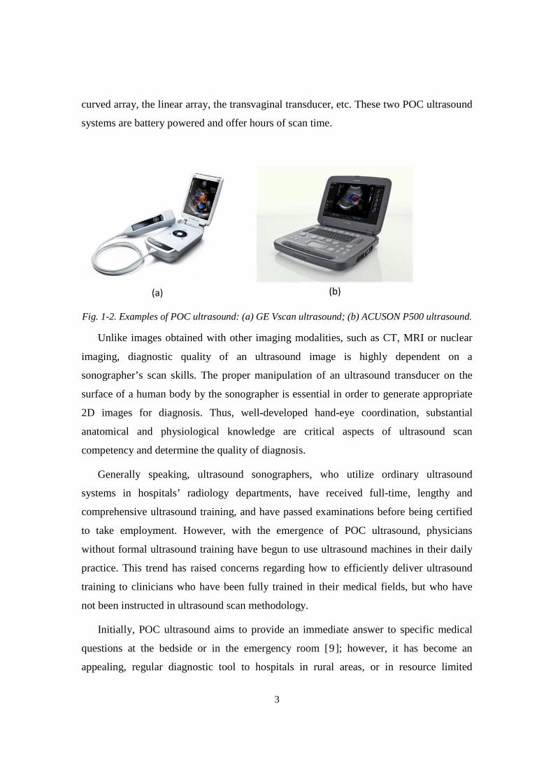
3

curved array, the linear array, the transvaginal transducer, etc. These two POC ultrasound

systems are battery powered and offer hours of scan time.

Fig. 1-2. Examples of POC ultrasound: (a) GE Vscan ultrasound; (b) ACUSON P500 ultrasound.

Unlike images obtained with other imaging modalities, such as CT, MRI or nuclear

imaging, diagnostic quality of an ultrasound image is highly dependent on a

sonographer’s scan skills. The proper manipulation of an ultrasound transducer on the

surface of a human body by the sonographer is essential in order to generate appropriate

2D images for diagnosis. Thus, well-developed hand-eye coordination, substantial

anatomical and physiological knowledge are critical aspects of ultrasound scan

competency and determine the quality of diagnosis.

Generally speaking, ultrasound sonographers, who utilize ordinary ultrasound

systems in hospitals’ radiology departments, have received full-time, lengthy and

comprehensive ultrasound training, and have passed examinations before being certified

to take employment. However, with the emergence of POC ultrasound, physicians

without formal ultrasound training have begun to use ultrasound machines in their daily

practice. This trend has raised concerns regarding how to efficiently deliver ultrasound

training to clinicians who have been fully trained in their medical fields, but who have

not been instructed in ultrasound scan methodology.

Initially, POC ultrasound aims to provide an immediate answer to specific medical

questions at the bedside or in the emergency room [9]; however, it has become an

appealing, regular diagnostic tool to hospitals in rural areas, or in resource limited

4

settings or low-income developing countries [ 10 , 11 ,12 , 13 ], largely due to POC

ultrasound’s merits, e.g. affordability, durability and portability. The widespread use of

POC ultrasound in these fields also eagerly demands efficient, affordable training

approaches to educate physicians, nurses and other clinical professionals.

1.1 Current Ultrasound Training

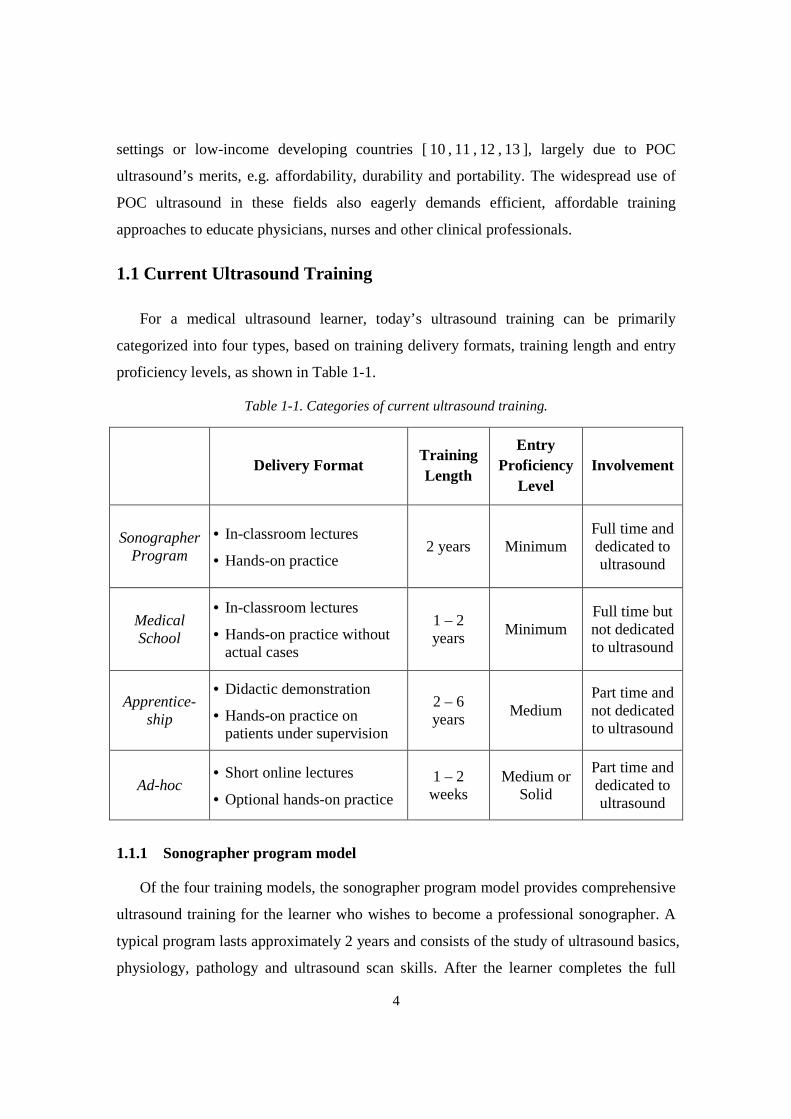
For a medical ultrasound learner, today’s ultrasound training can be primarily

categorized into four types, based on training delivery formats, training length and entry

proficiency levels, as shown in Table 1-1.

Table 1-1. Categories of current ultrasound training.

Delivery Format Training Length

Entry Proficiency

Level Involvement

Sonographer Program

• In-classroom lectures

• Hands-on practice 2 years Minimum

Full time and dedicated to ultrasound

Medical School

• In-classroom lectures

• Hands-on practice without actual cases

1 – 2 years

Minimum Full time but not dedicated to ultrasound

Apprentice-ship

• Didactic demonstration

• Hands-on practice on patients under supervision

2 – 6 years

Medium Part time and not dedicated to ultrasound

Ad-hoc • Short online lectures

• Optional hands-on practice

1 – 2 weeks

Medium or Solid

Part time and dedicated to ultrasound

1.1.1 Sonographer program model

Of the four training models, the sonographer program model provides comprehensive

ultrasound training for the learner who wishes to become a professional sonographer. A

typical program lasts approximately 2 years and consists of the study of ultrasound basics,

physiology, pathology and ultrasound scan skills. After the learner completes the full

5

time study, he or she needs to pass the examination offered by the American Registry for

Diagnostic Medical Sonography to obtain a certificate. Although the learner is not

required to have medical background to enroll these programs, a bachelor degree in any

discipline is preferred or the applicant must have studied a few specific college-level

courses. An ultrasound certificate program usually covers multiple specialties, including

obstetrics and gynecology, vascular ultrasound, cardiology, and abdominal ultrasound,

etc. Currently, there are many accredited sonographer programs in the Unites States, such

as the programs provided by the Middlesex Community College [14] and the Springfield

Technical Community College [15].

The sonographer program model has been the standard ultrasound training for

decades and it is absolutely able to provide the learner with effective training in the fields

of ultrasound hands-on and didactic ultrasound. However, this model is expensive,

lengthy and not appropriate for POC ultrasound learners, who usually have solid medical

knowledge and only want to utilize the ultrasound for promptly answering relatively

uncomplicated medical questions without involvement of radiologists.

1.1.2 Medical school model

Comparing to the other three models, the medical school model only requires the

learner to have minimum medical background. A good example is ultrasound curricula

provided by medical schools in recent years [16,17,18,19]. Ohio State University College

of Medicine (OSUCM) has developed an advanced ultrasound curriculum for their four-

year undergraduates [16]. It includes didactic lectures, journal clubs, hands-on practice,

and a final project. First and second year ultrasound courses gradually teach basic

ultrasound physics, knobology and protocols. The third and fourth year courses are

focused on ultrasound image acquisition and interpretation. Faculty members with solid

ultrasound experience in emergency medicine, internal medicine, obstetrics and

gynecology have been recruited to teach this curriculum.

In another published study, Wayne State University School of Medicine [17]

(WSUSM) has introduced a standardized ultrasound curriculum for first-year

undergraduates. This curriculum, spanning over one academic year, includes six 90-

minutes sessions covering ultrasound basic techniques and some procedural skills. Each

6

session contains didactic and hands-on practice. Similarly, Virginia et al. [18] and

Angtuaco et al. [19] have developed ultrasound curricula for medical school students

using instructional lectures and organ-specific hands-on practice.

The university programs that are focused on ultrasound basics and scan practice have

demonstrated positive outcomes in improving the beginners’ ultrasound skills. The

participants (medical school undergraduates) also expressed high level of satisfactions.

However, some limitations have been stated in above literature references [16,17,18,19].

Undergraduate ultrasound programs often face the challenge of limited availability of

ultrasound equipment and teaching faculty. Although the cost of a portable ultrasound

system (between $30,000 and $60,000) is lower than the cost of a larger stand-alone

ultrasound system, it is still costly for medical schools to acquire ultrasound machines in

sufficient quantity. Additionally, the lack of dedicated ultrasound faculty makes the

training less standardized and efficient because faculty members teach the courses based

on their preferences. Another major limitation of these university programs is that

undergraduates have very limited opportunities to exercise ultrasound skills in clinical

settings. Most of the time, they are only allowed to scan their partners during the training

sessions.

1.1.3 Apprenticeship Model

The apprenticeship model is usually focused on ultrasound hands-on practice and

actual case analysis under the assumption that the learner has already acquired the

required medical knowledge. Therefore, this model has been widely adopted in hospital

residency programs where a graduate continues developing his or her clinical skills

within a specific field after completing medical school. The learner, however, still needs

to take lengthy training sessions before he or she is competent in performing ultrasound

examination and making diagnosis. This is largely because the traditional apprenticeship

model is “see one, do one, teach one”. Only when an instructor, a patient scheduled for an

ultrasound scan, and an ultrasound system are ready, the learner will have the chance to

receive the training and practice scan skills. Unpredictable scan opportunities make the

ultrasound training less efficient.

7

According to a recent study that surveyed a number of directors of ultrasound training

programs for obstetrics and gynecology resident doctors [20], most of the programs

primarily relied on observation (sonographers’ demonstration) and hands-on practice to

improve ultrasound skills. These program directors have agreed that the learning

obstacles mainly resulted from the limited teaching resources, i.e., the lack of ultrasound

training opportunities and experienced faculty members. Many directors also expressed

the opinion that standard ultrasound training and competency assessment would best

facilitate resident doctors’ learning.

As the importance of structured ultrasound training becomes increasingly accepted,

some resident programs have begun to investigate the training curriculum’s impact to

training efficiency. In a recently published article [21], Beaulieu et al. evaluated the

effectiveness of web-based E-learning and hands-on training in a resident program at the

University of Montreal. In this experiment, one group of residents received the traditional

apprenticeship training whereas another group of residents received an added curriculum

in addition to the apprenticeship training. The added curriculum was delivered in the

form of formal courses, which combined self-directed E-learning lectures and a number

of hands-on sessions. The training lectures were delivered in different multimedia

formats, e.g. videos and slides, and via module-based approach. Their experiment showed

that the residents receiving the added curriculum performed ultrasound scan more

proficiently than those who only took traditional apprenticeship training. Another report

has reached the similar conclusion [22]. The obstetrics and gynecology department of

Doctors Hospital (Columbus, Ohio) integrated an ultrasound curriculum into their

residency program, which included reading programs, supervised hands-on scan and

didactic educational lectures. They found the residents taking integrated curriculum

performed more proficiently than those who only experienced standard OB/GYN

programs or one-month ultrasound rotation without sonographer guidance.

Although the apprenticeship model with a structured program has been proven useful

in improving ultrasound scan skills, it still faces the challenge that an inexperienced

resident doctor occasionally performs ultrasound scan in complicated environments

without sufficient supervision. This has raised the concern that patient safety may be

compromised [23].

8

1.1.4 Ad-hoc Model

Currently, the majority of POC ultrasound learners are physicians, nurses or clinical

professionals who have solid medical background. For them, the other three models

cannot meet their needs of completing ultrasound training via a short but efficient

program. The ad-hoc trainings may resolve this dilemma in some degree. It has multiple

formats, ranging from comprehensive short-term programs to online training courses.

E-learning and online courses [ 24 ] are widely available and affordable to the

clinicians who want to learn medical ultrasound. But this type of training is not suitable

to a novice user such as a physician with little or no ultrasound experience. The lack of

standard training procedure and scan practice make it inadequate to provide effective

ultrasound training to those people.

The short-term ultrasound program [25,26] condenses lectures, case study and hands-

on practice into a program lasting over a few days or weeks so that learner can complete

the training in a short time. Instead of certificates, acknowledged credits are given to the

learner who successfully completes such programs. The Gulfcoast Ultrasound Institute

[25], for example, offers a broad range of one-week full-time courses, covering major

specialties that often use ultrasound machines, such as obstetrics and gynecology,

emergency medicine, internal medicine, etc. The program is structured with lectures,

clinical studies and optional ultrasound scan practice (additional charges) on paid

volunteers. The participant should have some level of medical background to be suitable

for this intensive training, but it is not mandatory for the admission. The program is also

open to the people with little or no medical experience.

The ad-hoc training programs indeed are more flexible, affordable and accessible than

the other three models in delivering ultrasound training; however, the learner is less likely

to absorb ultrasound skills with limited hands-on opportunities and no continuing practice.

1.1.5 Challenges in current ultrasound training

The above four models each have their own advantages and disadvantages in

relationship to the POC ultrasound training. The apprenticeship model and the medical

school model progressively teach ultrasound skills over a long period so that the learner

9

has sufficient time to absorb the acquired knowledge and experience. These two models

are more appropriate for those who have little or some level of medical knowledge. The

short terms training programs (ad-hoc) has been proven relatively effective for physicians

or practitioners who have solid medical background to master basic ultrasound skills [10].

However, all four models share some common shortcomings, as stated below.

• Limited hands-on opportunities. The scan practice is believed to be the most critical

part of the ultrasound training and directly influences final training outcomes, because

learning ultrasound is a mental procedure often referred to as psychomotor training. A

number of studies [10, 20, 27] have proven that sufficient practice is necessary for

mastering ultrasound scan skills.

• Limited number of teaching faculty. In ultrasound training, 2D image acquisition and

interpretation are to some extent dependent on an instructor, whose competence

directly influences the training result. Almost all ultrasound programs employ in-

service faculty members or sonographers to teach the training. The lack of dedicated

instructors may make the training quality inconsistent and the training outcome less

satisfactory.

• High cost of training equipment. Although POC ultrasound systems are priced

significantly lower than the larger stand-alone ultrasound systems, it is still costly to

purchase sufficient number of ultrasound machines for educational institutions, not to

mention personal ownership of a training device.

1.2 Simulation Technology in Ultrasound Training

The expanding use of POC ultrasound systems requires a more efficient, affordable

training approach. Over the past decades, many published studies have proven the

efficacy and robustness of simulators in ultrasound training and promoted the adoption of

Simulation Based Medical Education (SBME). A recent survey [28] shows that 64

teaching hospitals and 90 medical schools have been utilizing simulation technology in

their programs and obstetrics has been one of the specialties utilizing simulation widely.

Besides the hands-on training, another major use of simulators in these programs was

competency assessment, primarily in the form of feedback. In obstetrics, the simulation

10

has been used in showing how to handle delivery emergencies [29] and perform prenatal

examination [ 30 ]. A 5-year study [ 31 ] has also shown that simulators have been

increasingly used in emergency medicine education. Of the 134 programs that responded

the survey, 122 programs used simulation in their education.

In addition to the decent learning effectiveness, the simulation technology also creates

a safe and supportive learning environment [32] where the learner can practice his or her

skills before applying them to actual patients. The Agency for Healthcare Research and

Quality (AHRQ) has promoted the development of simulation technology through its

patient safety program for a long time (PAR-11-024).

1.2.1 Effectiveness of simulator based ultrasound training

The learning-effectiveness of ultrasound simulator-based training has been

extensively studied and many researches have reported that ultrasound simulators can

efficiently train inexperienced users as well as or even better than conventional

ultrasound training in many specialties [33], such as obstetrics/gynecology [30,34,35],

emergency medicine [36], cardiology [37] and others [38,39].

In [40], the authors reviewed more than 100 simulator-related studies and concluded

that high-fidelity medical simulators can provide educationally effective medical

education. Another review study [ 41 ] reached a similar conclusion regarding the

simulator based education in obstetrics.

Several studies have demonstrated the learning effectiveness of ultrasound simulator-

based training in diagnostic ultrasound. One study evaluated the effectiveness of a

multimedia ultrasound simulator in a course of the Focused Assessment with Sonography

for Trauma (FAST) [42]. The experimental data indicated that the skills learned in

simulated training could be directly applied to human subjects. In [30], Maul et al.

conducted an experiment based on the SonoTrainer simulator. Their post-experiment

survey showed that 96% of participants thought that the training effect was good and the

hands-on training based on the simulator significantly improved their actual ultrasound

performance. The study [35] completed by Burden et al. reached a similar conclusion and

found that obstetricians with little experience could significantly improve their ultrasound

11

skills and biometric measurement accuracy and speed with short-term virtual reality

based training.

The effectiveness of simulator-based training in ultrasound guided procedures has

similarly been validated. In one study [43], 30 trainees received amniocentesis procedure

training based on a simulator, where the learner used a needle to sample amniotic fluid

from the uterus. The result showed that the simulator was effective in improving clinician

skills. Another recent study concluded that simulation plus didactic training in

ultrasound-guided central venous catheter insertion was superior to didactic training

alone for learning aseptic technique; after receiving combined training, novices

outperformed experienced resident doctors in the knowledge of aseptic technique and

measurement [44]. The clear benefits of transoesophageal echocardiography, using two

different commercial simulators, were also described in recent publications [45, 46].

1.2.2 Phantom-based and computer-based simulators

Generally, there are two major types of ultrasound simulators, either phantom-based

or computer-based. Up to now, the phantom-based simulators are still the primarily

training tool in SBME, especially in ultrasound guided intervention training. The

phantoms are made from materials that mimic the acoustic and physical properties of

human soft tissues, e.g. foam, gel, agar, rubber and gelatin.

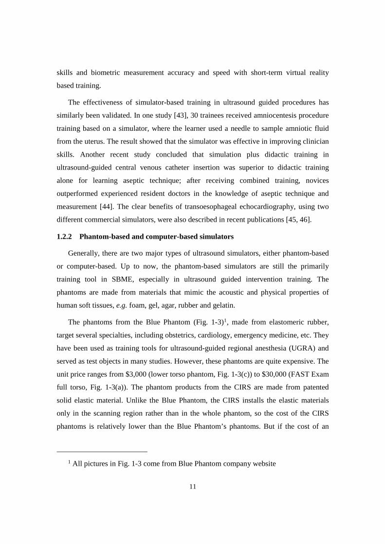
The phantoms from the Blue Phantom (Fig. 1-3)1, made from elastomeric rubber,

target several specialties, including obstetrics, cardiology, emergency medicine, etc. They

have been used as training tools for ultrasound-guided regional anesthesia (UGRA) and

served as test objects in many studies. However, these phantoms are quite expensive. The

unit price ranges from $3,000 (lower torso phantom, Fig. 1-3(c)) to $30,000 (FAST Exam

full torso, Fig. 1-3(a)). The phantom products from the CIRS are made from patented

solid elastic material. Unlike the Blue Phantom, the CIRS installs the elastic materials

only in the scanning region rather than in the whole phantom, so the cost of the CIRS

phantoms is relatively lower than the Blue Phantom’s phantoms. But if the cost of an

1 All pictures in Fig. 1-3 come from Blue Phantom company website

12

ultrasound machine is included, the price of the phantom-based training system

skyrockets.

Fig.1-3. The Blue Phantoms: (a) full torso; (b) upper torso; (c) lower torso.

In addition, commercial phantoms do not provide a realistic level of anatomical

details, which are often important to ultrasound training. Some of the larger phantoms are

cumbersome and thereby making simulation systems less portable.

An alternative are computer-based simulators, which create 2D ultrasound images

based on 3D image volumes stored in computers, instead of scanning phantoms to

generate 2D images. These 3D image volumes may either consist of directly acquired

ultrasound data or CT/MR image data processed to look somewhat like ultrasound data.

Consequently, a real ultrasound machine is not used in the training. There are currently

different approaches to build computer-based simulators, but they can be mainly

classified into four categories in terms of the image-generation approaches [47], as listed

below:

1) 3D ultrasound image volume based approach. The simulator directly extracts 2D

images, using interpolative algorithms, from 3D ultrasound image volumes that are

commonly acquired by scanning human subjects.

2) Deformable mesh model based approach. This type of simulators synthesizes

ultrasound images by simulating ultrasound wave propagation in deformable meshes

that integrate tissue elastic properties.

3) ‘Ultrasonified’ 3D image based approach. Instead of using 3D ultrasound image

volumes, this method creates 2D images based on 3D MR or CT image volumes. The

13

generated images are made to resemble ultrasound images by adding speckle noise

and shadows.

4) Mathematical model based approach. This method creates and textures 2D

ultrasound images using mathematic models. This approach is usually used when

anatomical structures of interest are too small to provide detailed tissue structure

information or moving too fast during data acquisition.

The above the four approaches have their own advantages and disadvantages for

implementing an ultrasound simulator. In the third approach, the ‘ultrasonified’ 3D image

volumes typically display the boundaries too well-defined and lacks shadowing artifacts

[48,49] to resemble actual 2D ultrasound images. But a large amount of readily available

3D image volumes make this approach attractive to developers. The deformable model

based approach retains some level of diffraction and shadowing effects pertaining to

actual ultrasound images. Nevertheless, it is currently too computationally demanding to

simulate complex tissue structures [ 50 ]. The mathematical based approach indeed

provides details in small organs or fast moving structures, but the generated images are

less realistic and the mathematical models need further verification. Compared to the

other approaches, the 3D ultrasound images based approach normally offers a higher

level of realism with acceptable computational requirements. Therefore, it is currently the

most common approach used by academic researchers to build an ultrasound simulator.

1.3 Review of Computer-Based Ultrasound Simulators

Currently, there are several commercial computer-based ultrasound simulators made

by different companies, such as MedSim, CAE healthcare, Simbionix and SonoSim. In

addition, many universities have developed, or are developing new simulators that are

more portable, affordable and user friendly.

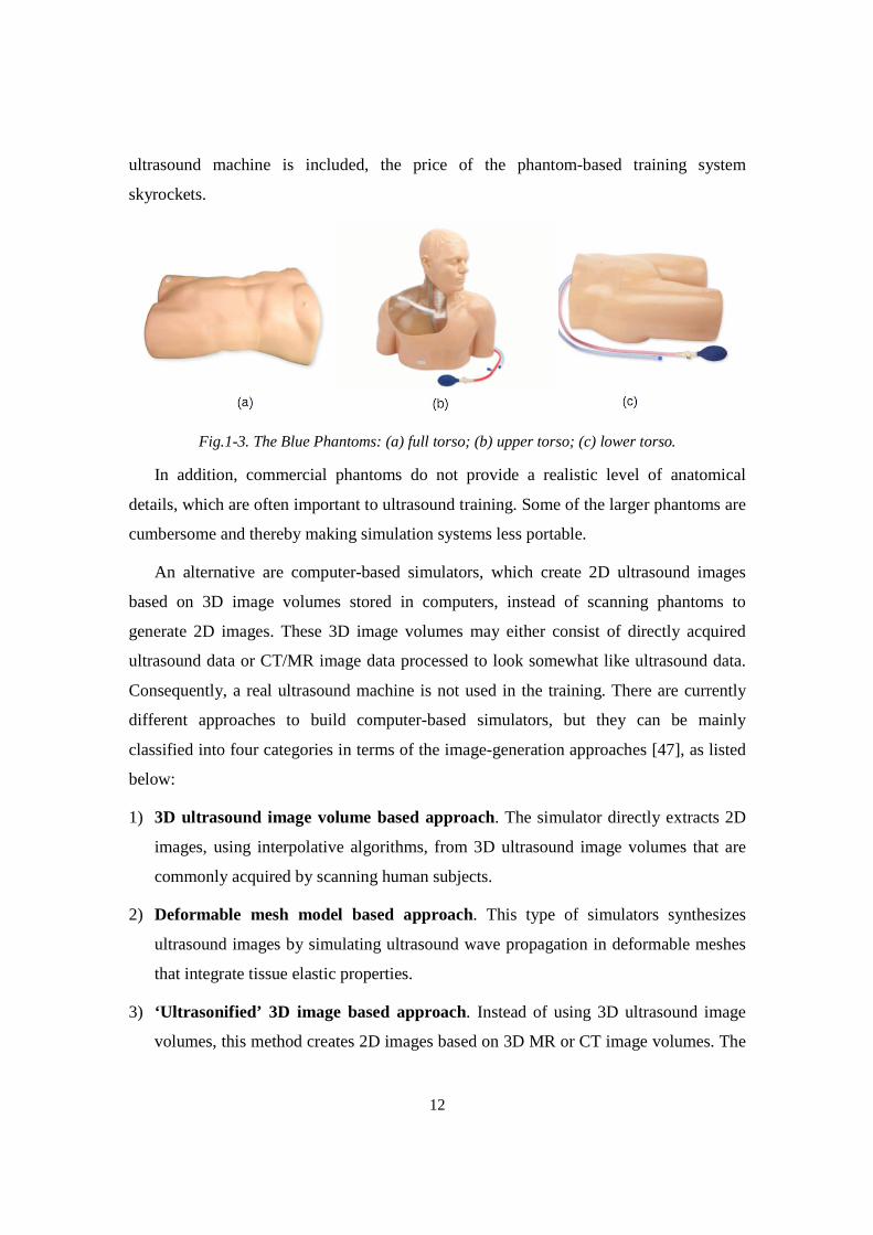
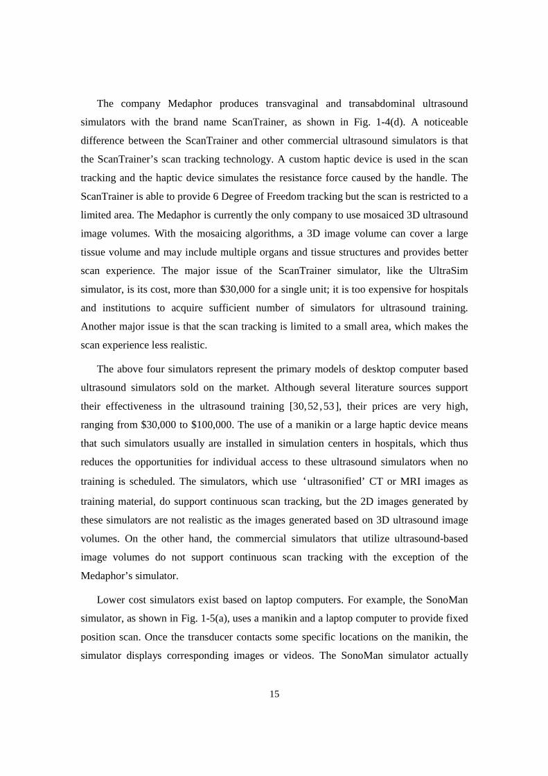
The UltraSim simulator [51 ], made by the MedSim, is the pioneer of modern

computer-based simulators, with the first product dating back to 1998. The system is

composed of a manikin, a sham ultrasound console and a sham transducer, as shown in

Fig. 1-4(a). The system is able to track the orientation of the transducer and then generate

and display 2D images in real-time based on a 3D ultrasound image volume. The

14

UltraSim simulator currently provides different training image volumes, covering a broad

range of medical specialties, such as obstetrics, ER medicine and gynecology. However,

the lack of extended 3D ultrasound image volumes and the sham transducer’s limitations

make the UltraSim simulator only able to support scan tracking with a limited degree of

realism. Users are unable to see continuous 2D images while they are scanning a large

region of the manikin. Also, the price of a stand-alone UltraSim unit is too expensive (up

to $100,000) to be standard training equipment for most of educational institutions.

The VIMEDIX simulator from CAE Healthcare, with a head-to-pelvis manikin, is

focused on visualizing the thoraxes, abdomens and pelvises using a sham transducer, as

shown in Fig. 1-4(b). This product aims to deliver ultrasound training for

echocardiography as well as ultrasound exams for lungs and pleural space and FAST

exam. Another CAE product offers obstetrics and gynecology training with a different

manikin. Learners can develop their skills in acquiring 2D images, locating anatomical

structures and performing biometric measurements. The VIMEDIX simulator visualizes,

on a split screen, anatomical structures on one side of the screen and the 2D images on

the other. In addition to providing B-mode ultrasound images, the VIMEDIX simulator

also supports M-mode and Doppler mode, and allows users to adjust gain and scan depth.

However, their products simulate the 2D images based on mathematical models or CT

dataset rather than 3D ultrasound image volumes. This makes the generated 2D images

less realistic.

The U/S Mentor simulator, manufactured by Simbionix, aims to teach basic

ultrasound skills in multiple areas, such as echocardiography, abdominal exam, FAST

exam and obstetrics. The whole system includes a manikin, a sham transducer and a big-

screen monitor (all-in-one desktop), as shown in Fig 1-4(c). An appealing feature of this

simulator is that a 3D anatomical model is displayed along with the 2D image on the

screen to help users observing the organs or tissues they are scanning. The orientation of

the 3D model can be manipulated by the user to achieve the best observation view.

Similar to the VIMEDIX simulator, the U/S Mentor simulator uses 3D CT image

volumes to simulate 2D ultrasound images.

15

The company Medaphor produces transvaginal and transabdominal ultrasound

simulators with the brand name ScanTrainer, as shown in Fig. 1-4(d). A noticeable

difference between the ScanTrainer and other commercial ultrasound simulators is that

the ScanTrainer’s scan tracking technology. A custom haptic device is used in the scan

tracking and the haptic device simulates the resistance force caused by the handle. The

ScanTrainer is able to provide 6 Degree of Freedom tracking but the scan is restricted to a

limited area. The Medaphor is currently the only company to use mosaiced 3D ultrasound

image volumes. With the mosaicing algorithms, a 3D image volume can cover a large

tissue volume and may include multiple organs and tissue structures and provides better

scan experience. The major issue of the ScanTrainer simulator, like the UltraSim

simulator, is its cost, more than $30,000 for a single unit; it is too expensive for hospitals

and institutions to acquire sufficient number of simulators for ultrasound training.

Another major issue is that the scan tracking is limited to a small area, which makes the

scan experience less realistic.

The above four simulators represent the primary models of desktop computer based

ultrasound simulators sold on the market. Although several literature sources support

their effectiveness in the ultrasound training [30,52,53], their prices are very high,

ranging from $30,000 to $100,000. The use of a manikin or a large haptic device means

that such simulators usually are installed in simulation centers in hospitals, which thus

reduces the opportunities for individual access to these ultrasound simulators when no

training is scheduled. The simulators, which use‘ultrasonified’ CT or MRI images as

training material, do support continuous scan tracking, but the 2D images generated by

these simulators are not realistic as the images generated based on 3D ultrasound image

volumes. On the other hand, the commercial simulators that utilize ultrasound-based

image volumes do not support continuous scan tracking with the exception of the

Medaphor’s simulator.

Lower cost simulators exist based on laptop computers. For example, the SonoMan

simulator, as shown in Fig. 1-5(a), uses a manikin and a laptop computer to provide fixed

position scan. Once the transducer contacts some specific locations on the manikin, the

simulator displays corresponding images or videos. The SonoMan simulator actually

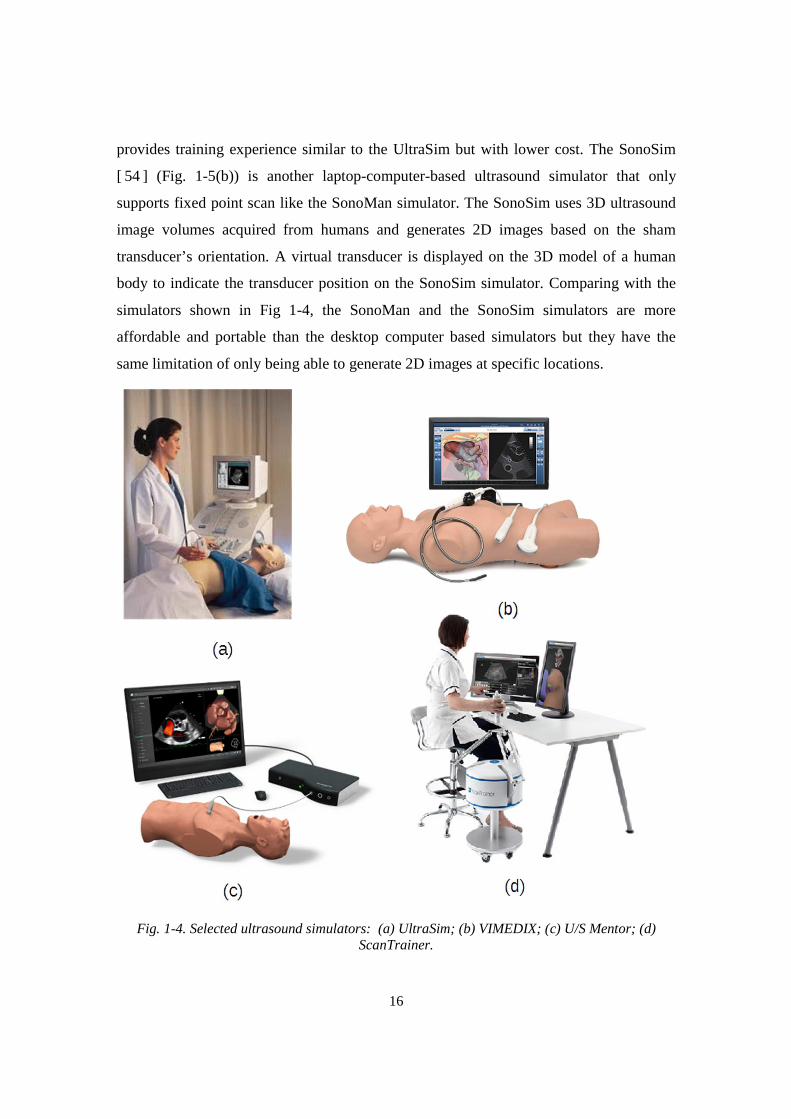
16

provides training experience similar to the UltraSim but with lower cost. The SonoSim

[ 54 ] (Fig. 1-5(b)) is another laptop-computer-based ultrasound simulator that only

supports fixed point scan like the SonoMan simulator. The SonoSim uses 3D ultrasound

image volumes acquired from humans and generates 2D images based on the sham

transducer’s orientation. A virtual transducer is displayed on the 3D model of a human

body to indicate the transducer position on the SonoSim simulator. Comparing with the

simulators shown in Fig 1-4, the SonoMan and the SonoSim simulators are more

affordable and portable than the desktop computer based simulators but they have the

same limitation of only being able to generate 2D images at specific locations.

Fig. 1-4. Selected ultrasound simulators: (a) UltraSim; (b) VIMEDIX; (c) U/S Mentor; (d) ScanTrainer.

17

Fig. 1-5. Laptop-computer-based ultrasound simulator: (a) SonoMan; (b) SonoSim.

In addition to commercial simulators, a few university-based efforts have resulted in

the development of ultrasound simulators in the past decade. In [50], the authors built a

deformable mesh based ultrasound simulator. Their experiment on simple objects, such

as spheroids and cylinders, showed that the simulated images were visually close to

actual ultrasound images. However, in their attempt to create ultrasound images of

complex objects, the computation increased exponentially due to the very large number

of mesh primitives needed to describe those complex objects. The processing was

impossible to complete on a personal computer even after a part of the calculation had

been moved to a Graphic Processing Unit (GPU). Thus, only objects with simple

geometries could be simulated in real-time. Kutter et al. [55] developed an ultrasound

simulator based on CT image volumes. This simulator was able to, on a split screen,

display ultrasound 2D images, which were processed by adding speckles and noise, on

the right screen, and display 3D anatomical structures on the left screen. Similarly, this

simulator required the use of a high-end GPU card2 to achieve real-time simulation and

visualization. Perk Tutor [56], an ultrasound guided needle insertion simulator based on

an open source platform, was developed for clinical practitioners. It could visualize

anatomical structures with 3D models on a computer and utilize another computer to

display 2D images generated from a phantom.

2 Quadro FX 5600 (1.5GB). This card is sold at the price of $300 in 2015.

18

1.4 The Need for An Affordable Computer-based Simulator for POC

Ultrasound Training

The need for POC ultrasound training is urgent, and there is a bigger demand for

training than can currently be met by traditional methods. We believe that ultrasound

simulators can offer an efficient and effective approach to meet POC ultrasound training

needs. The simulators provide a means for establishing and validating ultrasound training

standards. They can incorporate structured learning with progressively challenging

imaging tasks, and can assess the scan proficiency in a rigorous and consistent fashion.

After searching a number of published research literature and investigating the

commercial simulators, however, we found that these simulators do not provide POC

ultrasound users with effective and affordable training.

To meet the training need, an ultrasound simulator should, in addition to being

affordable, be able to facilitate the learning of ultrasound scan skills, such as image

acquisition, interpretation, and decision-making. As reviewed in the previous section, the

existing computer-based simulators have one or more limitations in meeting the POC

ultrasound training needs, such as high cost, not portable, absence of integrated training

curriculum and lacking a realistic simulation of the scan process. Therefore, we wished to

develop an ultrasound simulator suitable for personal ownership, with standard training

procedure and appropriate scan assessment. In this dissertation, we have chosen the

obstetric ultrasound training as the demonstration example.

1.5 The Dissertation Structure

This dissertation is organized based on the simulator components and the

implementation of obstetric ultrasound training. Chapter 2 presents an overview of the

design principles and the simulator structure. Next, Chapter 3 gives an overview of scan

tracking options and describes the design of the simulator’s scan tacking system.

Following this, Chapter 4 explains the approach used to generate an appropriate

mathematical model to map the abdominal surface of a given 3D image volume to the

generic physical scan surface of the scan tracking system. Chapter 5 presents the design

and structures of the simulator software as well as the implementation of the software

19

modules. A description of how to render a beating fetal heart is also given in this chapter.

In Chapter 6, the dissertation explains the design and implementation of obstetrics

ultrasound training tasks and the automatic scan assessment provided by the simulator.

With the training and assessment tools available, the learner is able to practice ultrasound

scan skills with the limited guidance from an instructor. Chapter 6 also covers the

algorithms to segment and to model fetal head and placenta in the 3D ultrasound image

volumes. The modeled anatomical structures are used by the simulator to evaluate if a

learner has successfully completed training tasks. Chapter 7 reviews the experiment that

evaluated the training efficacy and simulator performance. Twenty four 3rd year medical

students participated in the experiment. A set of data, including the completion time of

each task and each image volume, the usage of the help images and training videos, and

their subjective evaluation of the simulator, were collected and then analyzed. Chapter 8

presents the design of the ultrasound E-training system based on the networked simulator

described in this dissertation together with the test results of the system. Finally, the

conclusion and future work are presented in Chapter 9.

20

Chapter 2

Overview of the Simulator Design Principles and the

Simulator Features

In this chapter, we first describe four characteristics that we believe the ultrasound

training simulator should have. These four characteristics have formed the design

principles for the simulator. Then we give an overview of the simulator system (the

tracking system and the user interface), the generation of 3D training image volumes, the

training curriculum and scan assessment, and the E-training system based on the

networked simulators.

2.1 Four Characteristics of the New Ultrasound Simulator

An appropriate POC ultrasound training simulator should be able to facilitate

psychomotor learning of ultrasound scan skills, such as hand-eye coordination, image

interpretation, etc., with an affordable, efficient approach. To meet these requirements,

the new simulator should have four characteristics, as described below.

Affordability

As mentioned in Chapter 1, the key element in acquiring ultrasound skills is the

opportunity for large amount of hands-on practice. Using ultrasound simulators is a

possible solution to insufficient practice opportunities. However, simulator-based

ultrasound training has to date not been widely utilized due to the cost of ultrasound

simulators and training image volumes. Although laptop computer based simulators are

now available, they are still expensive to purchase for medical students, resident doctors

and clinical professionals. For medical professionals in developing countries, the cost of a

21

simulator for their hospital, let alone for personal ownership, is nearly prohibitive. To

make an ultrasound simulator affordable, design solutions must be found that utilize

inexpensive, yet reliable hardware components, primarily for tracking the sham

transducer. In addition, the simulator software must be suitable for common personal

computers. We have therefore set as a design goal to develop an ultrasound simulator

where the required hardware cost is only a few hundred dollars, in addition to the cost of

a computer on which the simulator software runs. This will allow simulator-based

ultrasound training to be a reality for a much wider group of medical students and

medical practitioners.

Realistic Scan Experience

Another critical factor that impacts the success of our obstetric ultrasound simulator is

whether the simulator can offer realistic scan experience, or free-hand scan, to a learner.

The obstetric ultrasound training cannot be performed simply by scanning at specific

positions on the abdomen of the simulator manikin. The psychomotor learning of scan

skills necessitates that the simulator must have ability to emulate free-hand scan. This

commonly requires that the scan tracking hardware of a simulator can acquire the

position and orientation of the transducer. In other words, the hardware should implement

5 DoF as a minimum, with 2 DoF for position and 3 DoF for orientation. Currently, a few

5 DoF or 6 DoF tracking systems have been made to offer free-hand scan. However, the

cost of such tracking hardware is expensive. Furthermore, all simulators having 6 DoF

tracking systems only utilize 3D CT image volumes to simulate 2D ultrasound images

and thereby provide less realistic training experience. For our simulator design, an

affordable scan simulation hardware supporting realistic scan experience is important.

Self-paced training curriculum and integrated assessment

Even though the efficacy and importance of simulator-based ultrasound training have

been widely recognized, its potential has not been fully utilized. The ultrasound training

is highly dependent on an instructor’s supervision and manual evaluation. The absence of

structured training procedures and simulator-based assessment in an ultrasound simulator

may be the primary obstacles that hinder the implementation of self-paced ultrasound

training.

22

Given that the American Institute of Ultrasound in Medicine (AIUM) has published

guidelines for standard obstetric ultrasound examination, the implementation of

structured training curriculum for an obstetric ultrasound simulator becomes feasible.

From a practical point of view, the design goal to incorporate self-paced training together

with automated assessment is made feasible by our ability to model anatomical structures

of training image volumes.

With appropriate structured training curriculum and automated assessment, the

learner is potentially less dependent on the availability of an instructor and thereby able

to more efficiently complete the ultrasound hands-on training.

Remote training for ultrasound scan skills

Another limitation of current ultrasound training programs is that training locations

are usually limited to medical schools or hospitals, which may be inconvenient for

learners living far away from such locations. To overcome the above restriction on

ultrasound training, it is a design goal that the obstetric ultrasound simulator would have

the ability to function in a network, allowing the implementation of a remote ultrasound

training system based on the networked simulators, by which anyone could participate

the training anywhere when communication networks are available. The new training

system will benefit ultrasound trainees who are living in the areas without training

centers or instructors.

2.2 Overview of the Simulator System

2.2.1 Implementation of the tracking system and simulator user interface

The ultrasound simulator has been designed to be a compact and affordable training

tool that can provide freehand scan. This requires the simulator to be primarily software

based. However, the simulator should also be able to realize the psycho-motor aspects of

diagnostic ultrasound training, that is, the manipulation of a physical sham transducer on

a body-like surface while make diagnostic decisions or biometric measurements on the

observed ultrasound image. Thus, the new simulator is intended to allow the learner to

scan over a particular part of human body corresponding with a specific ultrasound scan

protocol, such as obstetrics examination (the demonstration specialty in this dissertation).

23

This requires a physical scan surface, which approximately represents that particular

body area, and a 3D image volume, which must include anatomical and tissue structures

from that particular part of the human body. Such a large ultrasound image volume,

which for obstetric ultrasound includes most of the female abdomen, can only be

generated by stitching together several partially overlapping small 3D images that are

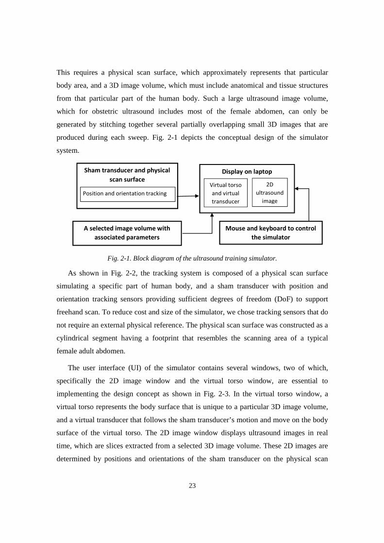
produced during each sweep. Fig. 2-1 depicts the conceptual design of the simulator

system.

Fig. 2-1. Block diagram of the ultrasound training simulator.

As shown in Fig. 2-2, the tracking system is composed of a physical scan surface

simulating a specific part of human body, and a sham transducer with position and

orientation tracking sensors providing sufficient degrees of freedom (DoF) to support

freehand scan. To reduce cost and size of the simulator, we chose tracking sensors that do

not require an external physical reference. The physical scan surface was constructed as a

cylindrical segment having a footprint that resembles the scanning area of a typical

female adult abdomen.

The user interface (UI) of the simulator contains several windows, two of which,

specifically the 2D image window and the virtual torso window, are essential to

implementing the design concept as shown in Fig. 2-3. In the virtual torso window, a

virtual torso represents the body surface that is unique to a particular 3D image volume,

and a virtual transducer that follows the sham transducer’s motion and move on the body

surface of the virtual torso. The 2D image window displays ultrasound images in real

time, which are slices extracted from a selected 3D image volume. These 2D images are

determined by positions and orientations of the sham transducer on the physical scan

Display on laptop Sham transducer and physical

scan surface 2D

ultrasound

image

Virtual torso

and virtual

transducer

Mouse and keyboard to control

the simulator

A selected image volume with

associated parameters

Position and orientation tracking

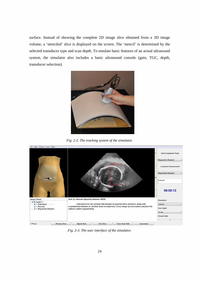
24

surface. Instead of showing the complete 2D image slice obtained from a 3D image

volume, a ‘stenciled’ slice is displayed on the screen. The ‘stencil’ is determined by the

selected transducer type and scan depth. To emulate basic features of an actual ultrasound

system, the simulator also includes a basic ultrasound console (gain, TGC, depth,

transducer selection).

Fig. 2-2. The tracking system of the simulator.

Fig. 2-3. The user interface of the simulator.

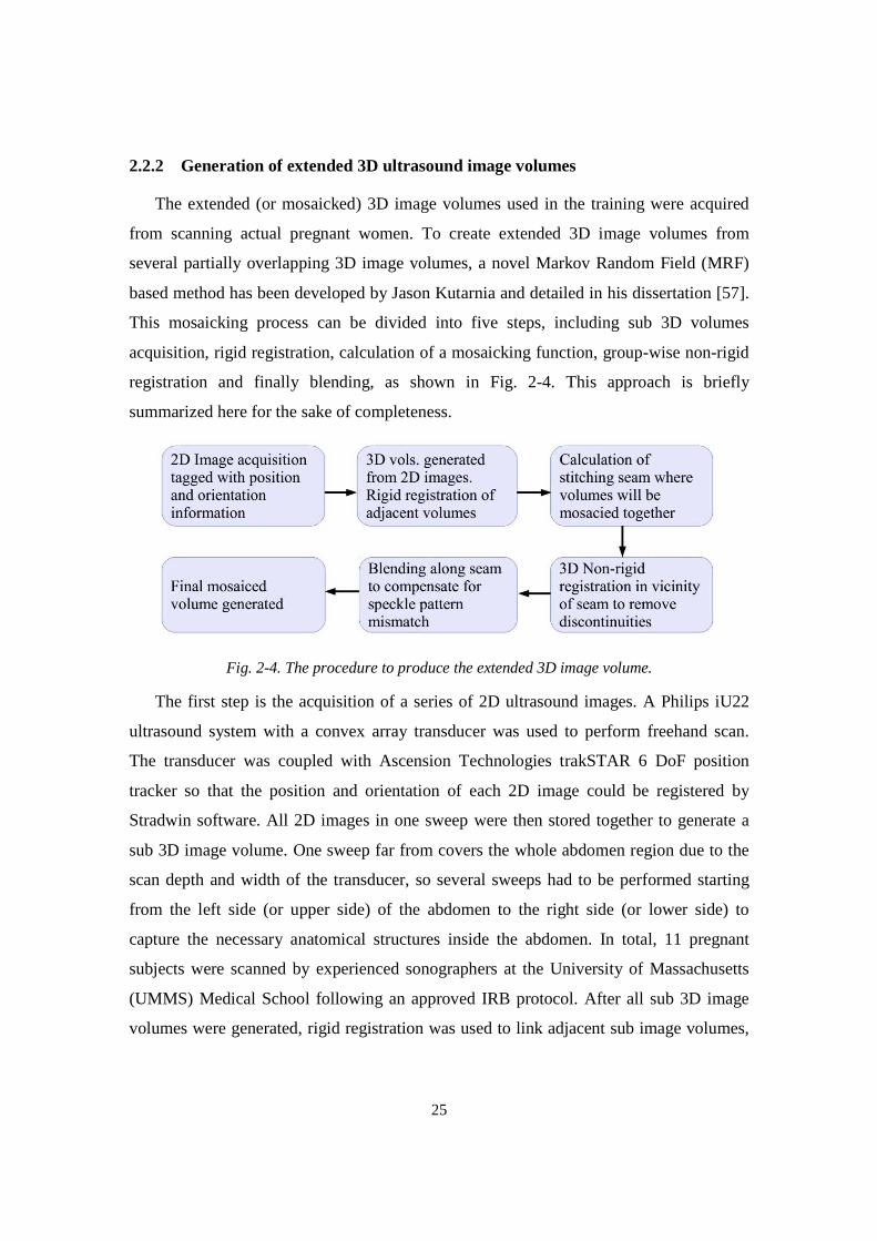
25

2.2.2 Generation of extended 3D ultrasound image volumes

The extended (or mosaicked) 3D image volumes used in the training were acquired

from scanning actual pregnant women. To create extended 3D image volumes from

several partially overlapping 3D image volumes, a novel Markov Random Field (MRF)

based method has been developed by Jason Kutarnia and detailed in his dissertation [57].

This mosaicking process can be divided into five steps, including sub 3D volumes

acquisition, rigid registration, calculation of a mosaicking function, group-wise non-rigid

registration and finally blending, as shown in Fig. 2-4. This approach is briefly

summarized here for the sake of completeness.

Fig. 2-4. The procedure to produce the extended 3D image volume.

The first step is the acquisition of a series of 2D ultrasound images. A Philips iU22

ultrasound system with a convex array transducer was used to perform freehand scan.

The transducer was coupled with Ascension Technologies trakSTAR 6 DoF position

tracker so that the position and orientation of each 2D image could be registered by

Stradwin software. All 2D images in one sweep were then stored together to generate a

sub 3D image volume. One sweep far from covers the whole abdomen region due to the

scan depth and width of the transducer, so several sweeps had to be performed starting

from the left side (or upper side) of the abdomen to the right side (or lower side) to

capture the necessary anatomical structures inside the abdomen. In total, 11 pregnant

subjects were scanned by experienced sonographers at the University of Massachusetts

(UMMS) Medical School following an approved IRB protocol. After all sub 3D image

volumes were generated, rigid registration was used to link adjacent sub image volumes,

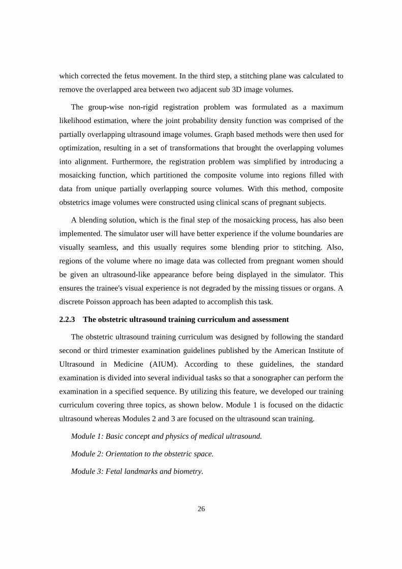
26

which corrected the fetus movement. In the third step, a stitching plane was calculated to

remove the overlapped area between two adjacent sub 3D image volumes.

The group-wise non-rigid registration problem was formulated as a maximum

likelihood estimation, where the joint probability density function was comprised of the

partially overlapping ultrasound image volumes. Graph based methods were then used for

optimization, resulting in a set of transformations that brought the overlapping volumes

into alignment. Furthermore, the registration problem was simplified by introducing a

mosaicking function, which partitioned the composite volume into regions filled with

data from unique partially overlapping source volumes. With this method, composite

obstetrics image volumes were constructed using clinical scans of pregnant subjects.

A blending solution, which is the final step of the mosaicking process, has also been

implemented. The simulator user will have better experience if the volume boundaries are

visually seamless, and this usually requires some blending prior to stitching. Also,

regions of the volume where no image data was collected from pregnant women should

be given an ultrasound-like appearance before being displayed in the simulator. This

ensures the trainee's visual experience is not degraded by the missing tissues or organs. A

discrete Poisson approach has been adapted to accomplish this task.

2.2.3 The obstetric ultrasound training curriculum and assessment

The obstetric ultrasound training curriculum was designed by following the standard

second or third trimester examination guidelines published by the American Institute of

Ultrasound in Medicine (AIUM). According to these guidelines, the standard

examination is divided into several individual tasks so that a sonographer can perform the

examination in a specified sequence. By utilizing this feature, we developed our training

curriculum covering three topics, as shown below. Module 1 is focused on the didactic

ultrasound whereas Modules 2 and 3 are focused on the ultrasound scan training.

Module 1: Basic concept and physics of medical ultrasound.

Module 2: Orientation to the obstetric space.

Module 3: Fetal landmarks and biometry.

27

The training in Modules 2 and 3 is composed of three steps. In step one, the learner

watches prerecorded a set of tutorial videos where a sonographer demonstrates ultrasound

scan skills and shows how each individual task is performed on the simulator. Then, in

step 2, the learner practices the scan skills by a series of training tasks, such as identifying

anatomical structures and completing biometric measurements, over a set of human

subjects (3D image volumes). After each task is completed, the simulator will assess if

the learner has correctly identified or measured the specified anatomical structures. In

step 3, the simulator evaluates the training performance using the exact same tasks in step

2 but on new 3D image volumes. The difference between the practice and test modes is

that the simulator provides feedback about wrong identification or measurement in the

practice mode while the test mode only gives the final result. Module 1 does not contain

step 2 (practice).

An essential component of the training simulator is its ability to automatically assess

whether the learner has correctly identified or measured a specified anatomical structure.

This is achieved by using a pre-inserted surface that surrounds, or bounds, the specified

structure at a close distance, where such a surface will be referred at as a ‘landmark

bound.’ Every training image volume has a number of landmark bounds, either registered

by experienced sonographers, or segmented and then modelled by algorithms.

2.2.4 The E-training system for ultrasound scan training

In a traditional obstetric ultrasound hands-on practice, a common scenario is one

where an instructor teaches a small group of learners by demonstrating and guiding the

scan on a pregnant subject using an ultrasound machine. Initially, the instructor

demonstrates the scan skills required to identify or measure the specific anatomical

structure(s) in question. Then, an individual learner may have a chance to perform the

scan under the instructor’s guidance after the demonstration. Ideally, all learners have the

opportunity to perform the scan by themselves with less supervision. Actually, this

typical ultrasound hands-on training can be mimicked based on the networked obstetric

ultrasound simulators, i.e., the E-training system. Such a system allows each training

participant to be instructed in the hands-on training at his/hers particular geographic

location. Based on the scenario described above, the training can be carried out by first

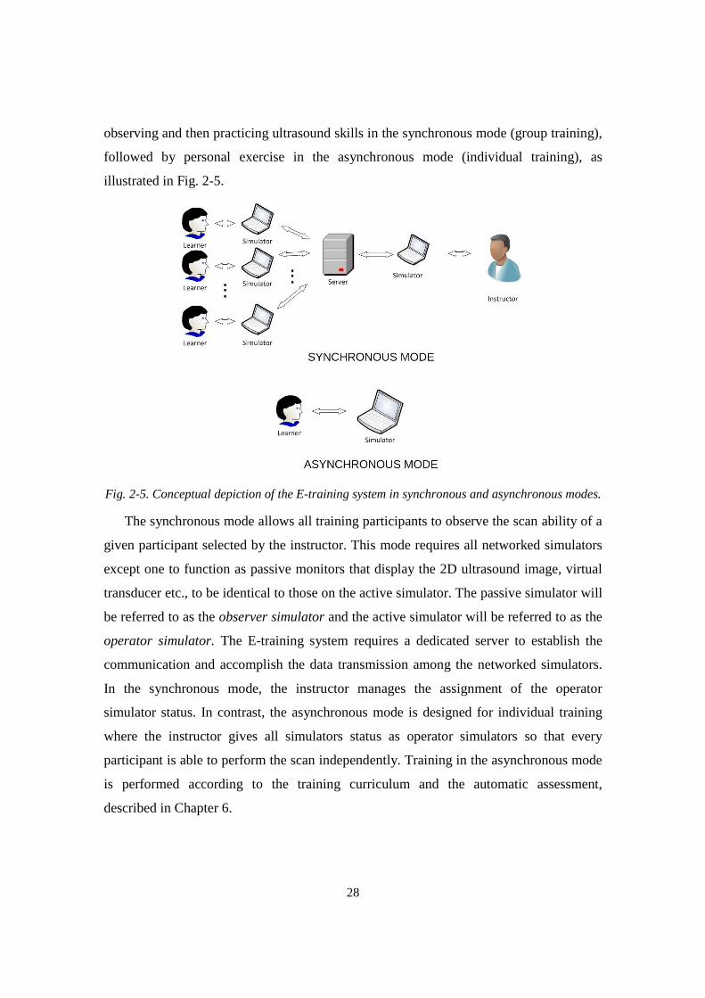
28

observing and then practicing ultrasound skills in the synchronous mode (group training),

followed by personal exercise in the asynchronous mode (individual training), as

illustrated in Fig. 2-5.

Fig. 2-5. Conceptual depiction of the E-training system in synchronous and asynchronous modes.

The synchronous mode allows all training participants to observe the scan ability of a

given participant selected by the instructor. This mode requires all networked simulators

except one to function as passive monitors that display the 2D ultrasound image, virtual

transducer etc., to be identical to those on the active simulator. The passive simulator will

be referred to as the observer simulator and the active simulator will be referred to as the

operator simulator. The E-training system requires a dedicated server to establish the

communication and accomplish the data transmission among the networked simulators.

In the synchronous mode, the instructor manages the assignment of the operator

simulator status. In contrast, the asynchronous mode is designed for individual training

where the instructor gives all simulators status as operator simulators so that every

participant is able to perform the scan independently. Training in the asynchronous mode

is performed according to the training curriculum and the automatic assessment,

described in Chapter 6.

29

Chapter 3

Design of the Scanning Tracking System

To design a new simulator supporting realistic scan experience, we must ensure that it

has the ability to track the instantaneous position and orientation of the sham transducer

relative to the physical scan surface, requiring 5 or 6 Degrees of Freedom3 (DoF) tracking

sensors. There are currently many position and orientation tracking devices available to

build a scan tracking system. Choosing appropriate, affordable sensors for the simulator

design is not trivial. In this chapter, we will give an overview of tracking devices that

have been used in the design of simulators and similar devices, explain sensor selection

criteria and implementation of the new simulator tracking system.

3.1 Overview of Motion Tracking Devices

In the past two decades, motion tracking devices had been widely used in many

applications, such as robot-assisted surgery systems [58,59], interactive entertainment

systems [60], and especially simulation systems [61,62]. Generally speaking, the motion

tracking is a process of capturing the position and orientation of objects in a specific

coordinate system. Entertainment systems use interactive means to encourage players to

more actively engage in the application. The growth of the Wii play station and the Xbox

Kinect has demonstrated appealing features of the motion tracking systems. On such

game consoles, a player utilizes his or her body movement to control the avatar in a game.

3 6 DoF refers to the freedom of the movement of an object in 3D coordinates. For

example, in Cartesian coordinates, an object can freely move and rotate around x, y or z

axes.

30

This particular experience offers two distinct advantages that cannot be provided by a

simple game handle: 1) it makes the player realistically play a role in a game to a large

extent and enhances his or her hand-eye coordination; 2) the player is more likely to

repetitively play the game.

An ultrasound simulation system requires its tracking system to have as few as 3 DoF

or as many as 6 DoF to detect the orientation and/or position of the sham transducer. For

example, normally, a manikin-based ultrasound simulators utilizes 6 DoF sensors in the

tracking system where a user scans the manikin following its contours of the body surface.

This method is absolutely not fit for our design goal due to its limitations, that is, non-

portable manikin and unaffordable tracking devices. It is also noticed that the simulators

with such 6 DoF tracking systems usually do not support tissue deformation. In other

words, a 5 DoF tracking system, 2 DoF for position tracking and 3 DoF for orientation

tracking, is sufficient to implement a manikin-based ultrasound simulator. A feasible

approach to reduce a tracking system’s cost is to combine multiple sensors to achieve

sufficient Degrees of Freedom. Currently, there are three major categories of tracking

systems [63] that have been widely used in simulators. They are the electro-magnetic, the

electro-optical and the electro-mechanical tracking systems.

3.1.1 Electro-magnetic Tracking Sensors

Compared to the other two categories of tracking systems, the Electromagnetic

Tracking System (EMTS) has a shorter development history, but it has been the most

widely used technology in the tracking system design. The EMTS is able to offer 6 DoF

tracking by means of a small sensor attached to the object to be tracked. The sensor

measures the flux of a magnetic field created by an electromagnetic transmitter to

interpret positions and orientations of the object.

Currently, there are two varieties of EMTS, implemented with either alternating

current (AC) or direct current (DC) pulsed magnetic fields. In the AC system, positions

and orientations of a sensor in the AC magnetic field are calculated based on the changes

of induced currents in the sensor itself [64], with a typical update frequency of 30 – 150

Hz. In contrast, the DC system uses a sequence of DC pulses, which turn the transmitter

on or off, to create a magnetic field [65]. There is a short delay between two adjacent

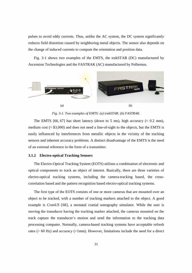
31

pulses to avoid eddy currents. Thus, unlike the AC system, the DC system significantly

reduces field distortion caused by neighboring metal objects. The sensor also depends on

the change of induced currents to compute the orientation and position data.

Fig. 3-1 shows two examples of the EMTS, the trakSTAR (DC) manufactured by

Ascension Technologies and the FASTRAK (AC) manufactured by Polhemus.

Fig. 3-1. Two examples of EMTS: (a) trakSTAR; (b) FASTRAK.

The EMTS [66, 67] has short latency (down to 5 ms), high accuracy (≈ 0.2 mm),

medium cost (≈ $3,000) and does not need a line-of-sight to the objects, but the EMTS is

easily influenced by interferences from metallic objects in the vicinity of the tracking

sensors and inherent accuracy problems. A distinct disadvantage of the EMTS is the need

of an external reference in the form of a transmitter.

3.1.2 Electro-optical Tracking Sensors

The Electro-Optical Tracking System (EOTS) utilizes a combination of electronic and

optical components to track an object of interest. Basically, there are three varieties of

electro-optical tracking systems, including the camera-tracking based, the cross-

correlation based and the pattern recognition based electro-optical tracking systems.

The first type of the EOTS consists of one or more cameras that are mounted over an

object to be tracked, with a number of tracking markers attached to the object. A good

example is CranUS [68], a neonatal cranial sonography simulator. While the user is

moving the transducer having the tracking marker attached, the cameras mounted on the

track capture the transducer’s motion and send the information to the tracking data

processing computer. Normally, camera-based tracking systems have acceptable refresh

rates (> 60 Hz) and accuracy (<1mm). However, limitations include the need for a direct

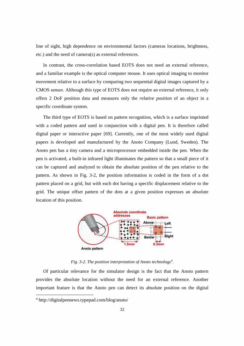
32

line of sight, high dependence on environmental factors (cameras locations, brightness,

etc.) and the need of camera(s) as external references.

In contrast, the cross-correlation based EOTS does not need an external reference,

and a familiar example is the optical computer mouse. It uses optical imaging to monitor

movement relative to a surface by comparing two sequential digital images captured by a

CMOS sensor. Although this type of EOTS does not require an external reference, it only

offers 2 DoF position data and measures only the relative position of an object in a

specific coordinate system.

The third type of EOTS is based on pattern recognition, which is a surface imprinted

with a coded pattern and used in conjunction with a digital pen. It is therefore called

digital paper or interactive paper [69]. Currently, one of the most widely used digital

papers is developed and manufactured by the Anoto Company (Lund, Sweden). The

Anoto pen has a tiny camera and a microprocessor embedded inside the pen. When the

pen is activated, a built-in infrared light illuminates the pattern so that a small piece of it

can be captured and analyzed to obtain the absolute position of the pen relative to the

pattern. As shown in Fig. 3-2, the position information is coded in the form of a dot

pattern placed on a grid, but with each dot having a specific displacement relative to the

grid. The unique offset pattern of the dots at a given position expresses an absolute

location of this position.

Fig. 3-2. The position interpretation of Anoto technology4.

Of particular relevance for the simulator design is the fact that the Anoto pattern

provides the absolute location without the need for an external reference. Another

important feature is that the Anoto pen can detect its absolute position on the digital 4 http://digitalpennews.typepad.com/blog/anoto/

33

paper even though the paper is placed on a curved surface [70]. This feature is critical to

our tracking system design because we require the coordinates of a specific point on the

paper must be absolute values. Such coordinates cannot be influenced by the orientation,

location and geometry of the paper.

3.1.3 Electro-mechanical Tracking Sensors

The electro-mechanical tracking systems exist in a broad range of implementations,

such as joysticks, spaceballs and haptic devices. In general, these devices detect the

position and orientation of an object by mechanically connecting the object to a reference

point.

The haptic device is an electro-mechanical sensor that simulates tactile feedback,

such as force, vibration and/or motion. Moreover, many haptic devices have ability to

track the movement of an object with high update rates (hundreds per second) and great

accuracy. This technology has been used in some ultrasound guided procedure simulators

and in most surgical simulators. For example, the ScanTrainer simulator utilizes a 6 DoF

haptic device, the Phantom Omni, to provide position and orientation data. However, the

cost of such a 6 DoF haptic device is high and thus not suited for an affordable ultrasound

simulator. In addition, the lack of ability to emulate free-hand scan makes haptic devices

improper for implementing an ultrasound simulator supporting realistic scan experience.

Inertial Measurement System (IMU) represents a different mechanical method that

enables orientation tracking by means of one or more gyroscopes. By using the earth’s

magnetic north and gravitational field as reference vectors, the IMU’s absolute

orientation in world coordinates can be obtained without drift. For example, the PNI

Fusion sensor consists of a 3-axis gyroscope, a 3-axis accelerometer and a 3-axis

geomagnetic sensors. This IMU provides rotation angle information (α,β,γ) along three

orthogonal axes in the form of quaternions, with a rate of 125 Hz and a resolution of

better than 0.1°. An integrated drift correct algorithm is implemented in the PNI sensor to

make it free of drift.

34

3.2 Requirements to Build a Tracking System Supporting Realistic Scan

To make an affordable simulator support realistic scan experience, the tracking

system should satisfy the following requirements:

• Degree of Freedom: be able to track 5 DoF position and orientation.

• Speed: provide tracking data more than 25 times per second to guarantee smooth

visual experience.

• Accuracy: measure the position and rotation angle with accuracy of better than 1

mm and 1°, respectively.

• Robustness: not affected by environmental factors.

• Cost and Portability: suitable for personal ownership.

• External reference: not accepted.

Based on the overview of the tracking technologies presented in the previous section

(with features summarized in Table 3-1), the only solution that meets all the requirements

stated above is a combination of an IMU and a pattern recognition based EOTS. All

current tracking technologies presented in the previous section meet the requirements of

accuracy and speed for the simulator’s tracking system. Thus, we selected the Anoto

digital paper and pen (Anoto AB, Lund, Sweden) and the PNI SpacePoint IMU sensor

(PNI Sensor Corp., Santa Rosa, CA), as the specific tracking components.

The combination of the Anoto pen and the PNI sensor offers 5 DoF of tracking ability,

2 DoF for position tracking and 3 DoF for orientation tracking. This is sufficient to

support realistic scan experience assuming that we do not consider the tissue compressive

force applied by the sham transducer to the scan surface. If an ultrasound simulator

existed for training in performing a prostate ultrasound exam, the detection of

compressive force should be included in the tracking system design, because a physician

depends on the deformation level of the prostate to predict the subject’s health condition.

For obstetrics ultrasound, tissue deformation also exists, but it is not a key factor to

determine training efficacy. Thus, without simulating tissue deformation, the new

tracking system only requires 5 DoF.

35

Table 3-1. The feature summary of the tracking systems.

3.3 Implementation of the Physical Scan Surface

To reduce the cost of the tracking system and provide realistic scan experience, the

design of the new simulator requires that the physical scan surface meets a few

requirements:

(1) The dimensions and geometry of the physical scan surface should be

approximately similar to the body surface to be scanned.

(2) Every point on the scan surface must have a well-defined position and surface

normal in a 3D Cartesian coordinate system.

(3) The physical scan surface must be easily transported, assembled and produced

with affordable materials.

(4) The physical scan surface should accommodate a surface printed with the Anoto

pattern.

For an obstetric ultrasound simulator, the physical scan surface should have

dimensions and geometries similar to the female abdomen. Therefore, we have chosen

DoF External

Reference Cost Adverse Impact

EMTS 6 Yes Expensive Result in distortion if the metal objects exist in the vicinity

Camera-based tracking system

6 Yes Expensive Need line of sight and subject to ambient factors

Optical Mouse 2 No Affordable Cannot provide absolute position

Digital Paper 2 No Affordable Not significant

IMU 3 No Affordable Not significant

Haptic Devices 2-6 No Expensive Cannot be used as a tracking device

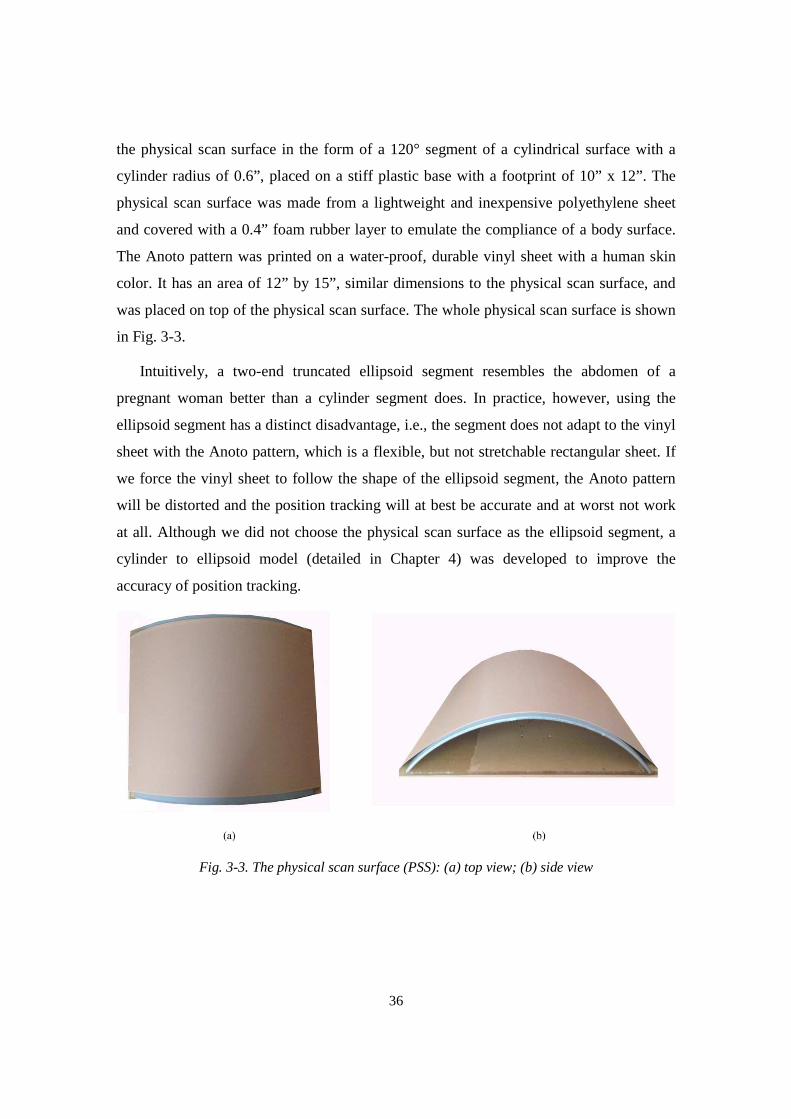
36

the physical scan surface in the form of a 120° segment of a cylindrical surface with a

cylinder radius of 0.6”, placed on a stiff plastic base with a footprint of 10” x 12”. The

physical scan surface was made from a lightweight and inexpensive polyethylene sheet

and covered with a 0.4” foam rubber layer to emulate the compliance of a body surface.

The Anoto pattern was printed on a water-proof, durable vinyl sheet with a human skin

color. It has an area of 12” by 15”, similar dimensions to the physical scan surface, and

was placed on top of the physical scan surface. The whole physical scan surface is shown

in Fig. 3-3.

Intuitively, a two-end truncated ellipsoid segment resembles the abdomen of a

pregnant woman better than a cylinder segment does. In practice, however, using the

ellipsoid segment has a distinct disadvantage, i.e., the segment does not adapt to the vinyl

sheet with the Anoto pattern, which is a flexible, but not stretchable rectangular sheet. If

we force the vinyl sheet to follow the shape of the ellipsoid segment, the Anoto pattern

will be distorted and the position tracking will at best be accurate and at worst not work

at all. Although we did not choose the physical scan surface as the ellipsoid segment, a

cylinder to ellipsoid model (detailed in Chapter 4) was developed to improve the

accuracy of position tracking.

Fig. 3-3. The physical scan surface (PSS): (a) top view; (b) side view

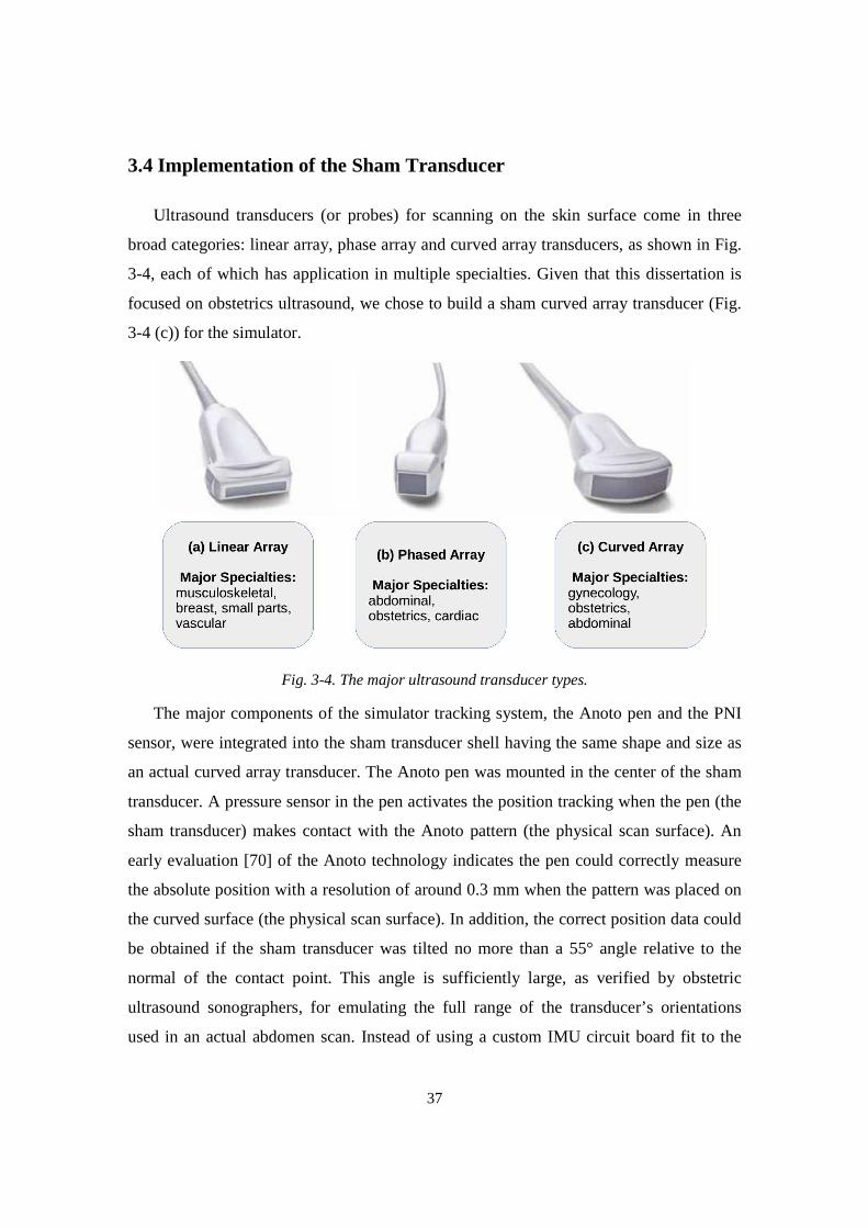
37

3.4 Implementation of the Sham Transducer

Ultrasound transducers (or probes) for scanning on the skin surface come in three

broad categories: linear array, phase array and curved array transducers, as shown in Fig.

3-4, each of which has application in multiple specialties. Given that this dissertation is

focused on obstetrics ultrasound, we chose to build a sham curved array transducer (Fig.

3-4 (c)) for the simulator.

Fig. 3-4. The major ultrasound transducer types.

The major components of the simulator tracking system, the Anoto pen and the PNI

sensor, were integrated into the sham transducer shell having the same shape and size as

an actual curved array transducer. The Anoto pen was mounted in the center of the sham

transducer. A pressure sensor in the pen activates the position tracking when the pen (the

sham transducer) makes contact with the Anoto pattern (the physical scan surface). An

early evaluation [70] of the Anoto technology indicates the pen could correctly measure

the absolute position with a resolution of around 0.3 mm when the pattern was placed on

the curved surface (the physical scan surface). In addition, the correct position data could

be obtained if the sham transducer was tilted no more than a 55° angle relative to the

normal of the contact point. This angle is sufficiently large, as verified by obstetric

ultrasound sonographers, for emulating the full range of the transducer’s orientations

used in an actual abdomen scan. Instead of using a custom IMU circuit board fit to the

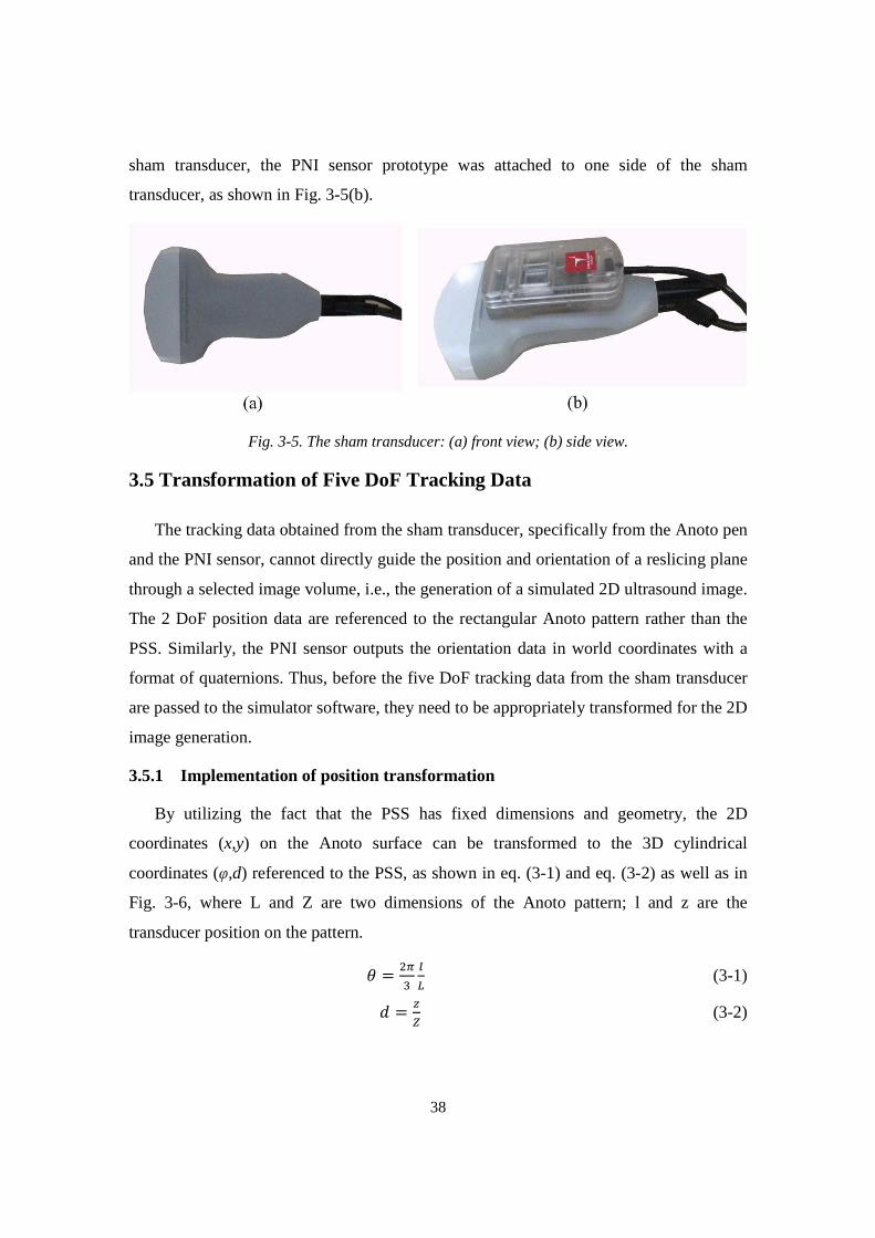
38

sham transducer, the PNI sensor prototype was attached to one side of the sham

transducer, as shown in Fig. 3-5(b).

Fig. 3-5. The sham transducer: (a) front view; (b) side view.

3.5 Transformation of Five DoF Tracking Data

The tracking data obtained from the sham transducer, specifically from the Anoto pen

and the PNI sensor, cannot directly guide the position and orientation of a reslicing plane

through a selected image volume, i.e., the generation of a simulated 2D ultrasound image.

The 2 DoF position data are referenced to the rectangular Anoto pattern rather than the

PSS. Similarly, the PNI sensor outputs the orientation data in world coordinates with a

format of quaternions. Thus, before the five DoF tracking data from the sham transducer

are passed to the simulator software, they need to be appropriately transformed for the 2D

image generation.

3.5.1 Implementation of position transformation

By utilizing the fact that the PSS has fixed dimensions and geometry, the 2D

coordinates (x,y) on the Anoto surface can be transformed to the 3D cylindrical

coordinates (φ,d) referenced to the PSS, as shown in eq. (3-1) and eq. (3-2) as well as in

Fig. 3-6, where L and Z are two dimensions of the Anoto pattern; l and z are the

transducer position on the pattern.

� = ��� �� (3-1)

� = (3-2)

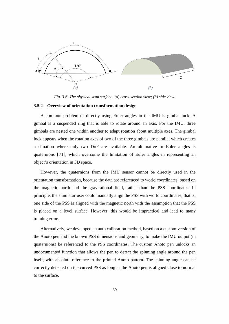
39

Fig. 3-6. The physical scan surface: (a) cross-section view; (b) side view.

3.5.2 Overview of orientation transformation design

A common problem of directly using Euler angles in the IMU is gimbal lock. A

gimbal is a suspended ring that is able to rotate around an axis. For the IMU, three

gimbals are nested one within another to adapt rotation about multiple axes. The gimbal

lock appears when the rotation axes of two of the three gimbals are parallel which creates

a situation where only two DoF are available. An alternative to Euler angles is

quaternions [71], which overcome the limitation of Euler angles in representing an

object’s orientation in 3D space.

However, the quaternions from the IMU sensor cannot be directly used in the

orientation transformation, because the data are referenced to world coordinates, based on

the magnetic north and the gravitational field, rather than the PSS coordinates. In

principle, the simulator user could manually align the PSS with world coordinates, that is,

one side of the PSS is aligned with the magnetic north with the assumption that the PSS

is placed on a level surface. However, this would be impractical and lead to many

training errors.

Alternatively, we developed an auto calibration method, based on a custom version of

the Anoto pen and the known PSS dimensions and geometry, to make the IMU output (in

quaternions) be referenced to the PSS coordinates. The custom Anoto pen unlocks an

undocumented function that allows the pen to detect the spinning angle around the pen

itself, with absolute reference to the printed Anoto pattern. The spinning angle can be

correctly detected on the curved PSS as long as the Anoto pen is aligned close to normal

to the surface.

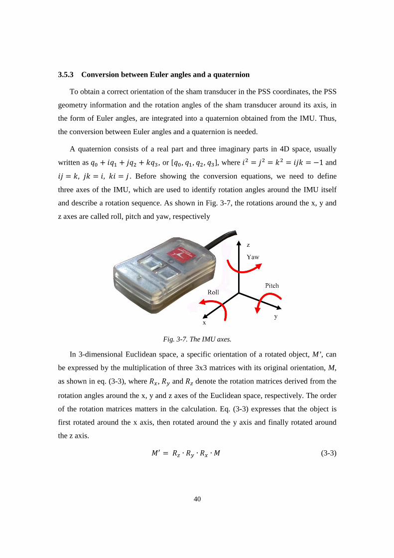
40

3.5.3 Conversion between Euler angles and a quaternion

To obtain a correct orientation of the sham transducer in the PSS coordinates, the PSS

geometry information and the rotation angles of the sham transducer around its axis, in

the form of Euler angles, are integrated into a quaternion obtained from the IMU. Thus,

the conversion between Euler angles and a quaternion is needed.

A quaternion consists of a real part and three imaginary parts in 4D space, usually

written as �� + ��� + ��� + ���, or [��,��,��,��], where �� = �� = �� = ��� = −1 and �� = �, �� = �, �� = � . Before showing the conversion equations, we need to define

three axes of the IMU, which are used to identify rotation angles around the IMU itself

and describe a rotation sequence. As shown in Fig. 3-7, the rotations around the x, y and

z axes are called roll, pitch and yaw, respectively

Fig. 3-7. The IMU axes.

In 3-dimensional Euclidean space, a specific orientation of a rotated object, M’ , can

be expressed by the multiplication of three 3x3 matrices with its original orientation, M,

as shown in eq. (3-3), where ��, �� and � denote the rotation matrices derived from the

rotation angles around the x, y and z axes of the Euclidean space, respectively. The order

of the rotation matrices matters in the calculation. Eq. (3-3) expresses that the object is

first rotated around the x axis, then rotated around the y axis and finally rotated around

the z axis.

�� =� ∙ �� ∙ �� ∙ � (3-3)

41

In this dissertation, we define the rotation order as first rotating the IMU around its y

axis, then around its z axis and finally around its x axis. Therefore, the equations for

converting a quaternion to the corresponding Euler angles are:

����ℎ = � !2(2 ∗ �2 ∗ �0 − 2 ∗ �� ∗ �3, ��� − ��� − ��� + ���) (3-4)

()** = � !2(2 ∗ �1 ∗ �0 − 2 ∗ �2 ∗ �3, −��� + ��� − ��� − ��� (3-5)

+ , = asin(2 ∗ �� ∗ �2 + 2 ∗ �3 ∗ �0) (3-6)

where ����ℎ, ()** and + , are defined in Fig 3-7; � !2 returns an angle between -π

and π; 1�! returns an angle between -π/2 and π/2. The above three equations are suitable

for calculating all rotation angles except for two conditions, that is, when the + ,

rotation equals to 90° or -90°. However, these two singular angles will never occur in the

simulator’s tracking system due to the geometric restriction of the physical scan surface

and the sham transducer.

The equations of converting Euler angels to a quaternion are shown below:

�0 = c1c2c3 − s1s2s3 (3-7)

�1 = s1s2c3 + c1c2s3 (3-8)

�2 = s1c2c3 + c1s2s3 (3-9)

�3 = c1s2c3 − s1c2s3 (3-10)

,ℎ3(345657c1 = cos 9pitch2 = , s1 = sin 9pitch2 =c2 = cos >yaw2 A , s2 = cos >yaw2 Ac3 = cos 9roll2 = , s3 = cos 9roll2 =

3.5.4 Implementation of the orientation transformation

In world coordinates, a special orientation occurs when the x and z axes of the IMU

points to the magnetic north and aligns with the gravity vector, respectively; this

orientation gives a quaternion with the value of (1,0,0,0). It is called identity quaternion,

and it is similar to an orientation that results in alignment along the major axes of 2D or

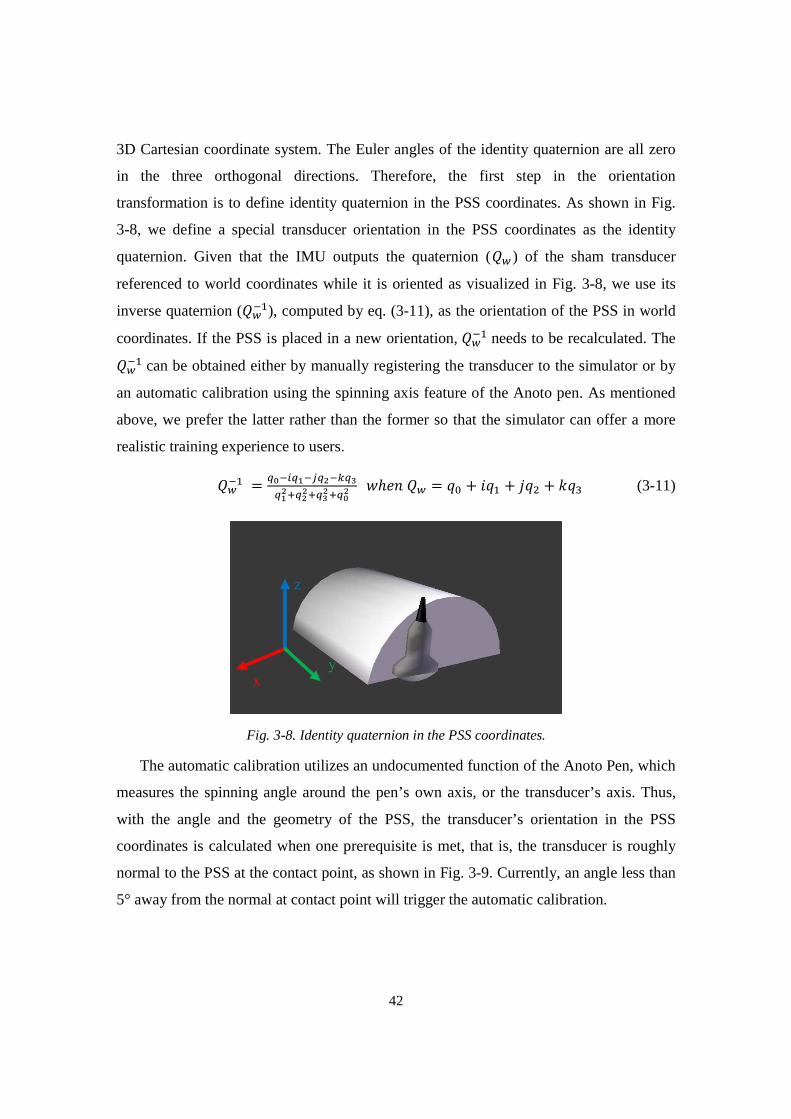
42

3D Cartesian coordinate system. The Euler angles of the identity quaternion are all zero

in the three orthogonal directions. Therefore, the first step in the orientation

transformation is to define identity quaternion in the PSS coordinates. As shown in Fig.

3-8, we define a special transducer orientation in the PSS coordinates as the identity

quaternion. Given that the IMU outputs the quaternion (DE ) of the sham transducer

referenced to world coordinates while it is oriented as visualized in Fig. 3-8, we use its

inverse quaternion (DEF�), computed by eq. (3-11), as the orientation of the PSS in world

coordinates. If the PSS is placed in a new orientation, DEF� needs to be recalculated. The DEF� can be obtained either by manually registering the transducer to the simulator or by

an automatic calibration using the spinning axis feature of the Anoto pen. As mentioned

above, we prefer the latter rather than the former so that the simulator can offer a more

realistic training experience to users.

DEF� = GHFIGJFKGLFMGNGJLOGLLOGNLOGHL ,ℎ3!DE = �� + ��� + ��� + ��� (3-11)

Fig. 3-8. Identity quaternion in the PSS coordinates.

The automatic calibration utilizes an undocumented function of the Anoto Pen, which

measures the spinning angle around the pen’s own axis, or the transducer’s axis. Thus,

with the angle and the geometry of the PSS, the transducer’s orientation in the PSS

coordinates is calculated when one prerequisite is met, that is, the transducer is roughly

normal to the PSS at the contact point, as shown in Fig. 3-9. Currently, an angle less than

5° away from the normal at contact point will trigger the automatic calibration.

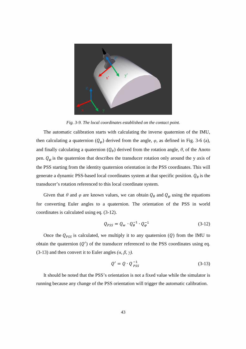
43

Fig. 3-9. The local coordinates established on the contact point.

The automatic calibration starts with calculating the inverse quaternion of the IMU,

then calculating a quaternion (DP) derived from the angle, φ, as defined in Fig. 3-6 (a),

and finally calculating a quaternion (DQ) derived from the rotation angle, θ, of the Anoto

pen. DP is the quaternion that describes the transducer rotation only around the y axis of

the PSS starting from the identity quaternion orientation in the PSS coordinates. This will

generate a dynamic PSS-based local coordinates system at that specific position. DQ is the

transducer’s rotation referenced to this local coordinate system.

Given that θ and φ are known values, we can obtain DQ and DP using the equations

for converting Euler angles to a quaternion. The orientation of the PSS in world

coordinates is calculated using eq. (3-12).

DRSS = DE ∙ DQF� ∙ DPF� (3-12)

Once the DRSS is calculated, we multiply it to any quaternion (D) from the IMU to

obtain the quaternion (D�) of the transducer referenced to the PSS coordinates using eq.

(3-13) and then convert it to Euler angles (α, β, γ).

D� = D ∙ DRSSF� (3-13)

It should be noted that the PSS’s orientation is not a fixed value while the simulator is

running because any change of the PSS orientation will trigger the automatic calibration.

44

3.5.5 Summary of tracking data transformation

The orientation and position transformation described in this section is part of the

sham transducer driver. The five DoF tracking data (θ,d,α,β,γ) need to be further

transformed from the PSS coordinates into a given 3D image coordinates using a

mathematical model generated offline (detailed in Chapter 5) before these data are used

to guide the simulator to extract 2D images from the 3D image volume.

45

Chapter 4

Mapping of 3D Image Volumes to Physical Scan Surface

The obstetric ultrasound simulator utilizes 3D ultrasound image volumes acquired

from actual pregnant women to generate 2D ultrasound images. Each pregnant woman

has a different abdominal geometry and therefore the abdominal surface of every 3D

image volume is unique. However, the dimensions and geometry of the Physical Scan

Surface (PSS) are fixed. As a result, the movements of the sham transducer on the PSS

cannot be directly used to generate 2D images from the given 3D image volume or to

guide the movement of the virtual transducer on the corresponding virtual torso. Thus a

mapping approach is required to match the positions of points on the abdominal surface

of a given 3D image volume to corresponding points on the PSS so that the orientation

and position of the sham transducer in the PSS coordinates can be correctly transformed

into the unique 3D image coordinates.

Usually, the geometry of the abdominal surface of a pregnant woman in the second

trimester approximates a truncated ellipsoid segment, that is, the surface obtained by

cutting an ellipsoid by a plane parallel to the major axis and then truncating at both ends

[72]. Therefore, we proposed an approach that creates a cylindrical Virtual Scan Surface

(VSS) and a truncated ellipsoidal Virtual Abdominal Surface (VAS) from a given3D

image volume to implement the mapping from the abdominal surface of the 3D image

volume to the PSS. The use of the VAS aims to improve the accuracy of the sham

transducer’s position transformation by making the transformed coordinates closer to the

abdominal surface in the coordinates of the 3D image volume. This cylinder-to-ellipsoid

model assists the simulator in transforming the five Degree of Freedom (DoF) tracking

data, as detailed Chapter 3, into the 3D image volume coordinates. In this chapter, we

46

will explain the approach used to extract the 3D abdominal surface from a given 3D

image volume and the method employed to generate the VSS and the VAS based on the

3D abdominal surface.

4.1 Extraction of the 3D Abdominal Surface for a 3D Image Volume

The main objective in the generation of an extended 3D image volume was the

alignment of fetal and maternal anatomical structures in the overlapping parts of adjacent

individual 3D image volumes [57]. This usually resulted in the abdominal surface of a

given 3D image volume being irregularly shaped. In other words, only a part of 3D image

volume surface could represent the actual abdominal surface of the pregnant woman.

This issue often caused difficulties in mapping the 3D abdominal surface to the PSS with

our proposed approach, such as lowering the mapping accuracy or even making the

mapping model impossible to generate. Thus, we needed to obtain the appropriate

abdominal surface suitable for the mapping before creating the VSS and the VAS.

The valid abdominal surface of a given 3D image volume was determined manually

by observing the whole image volume in a Matlab toolkit, SliceBrowser. Fig. 4-1 shows

an example of displaying a 3D image volume with 2D views. The background of the 3D

image volume is totally black (voxel value = 0), and any fetal and maternal tissues or

organs except fluid have voxel values between 1 and 255 (white).

In the xy and yz planes of Fig. 4-1, only part of the 3D image volume surface can be

considered to be the abdominal surface, but we are not able extract it by simply

truncating the 3D image volume along x, y and z axes and then detecting the first non-

zero value along the y axis of the 3D image volume coordinates. This approach was

originally used to capture the abdominal surface of the 3D image volume from The

Visible Human Project [70], but it had been proven not appropriate for the extended 3D

image volumes in our early evaluation, as it often led to an incomplete abdominal surface

or excessive tissues included in the abdominal surface.

Therefore, instead of determining the abdominal surface based on 2D images, we

created the isosurface, or mesh, of the given 3D image volume, with Fang’s algorithm

[73], and then determined the abdominal surface in Blender, a 3D graphics and animation

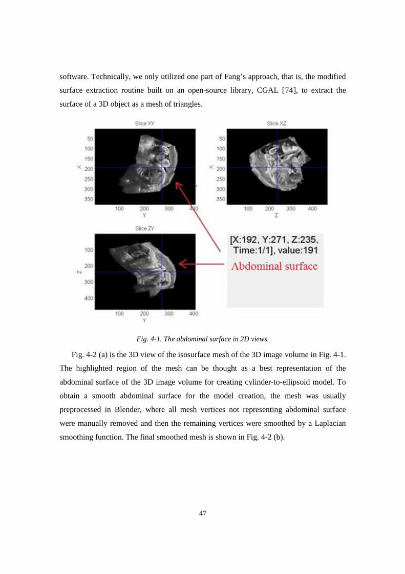
47

software. Technically, we only utilized one part of Fang’s approach, that is, the modified

surface extraction routine built on an open-source library, CGAL [74], to extract the

surface of a 3D object as a mesh of triangles.

Fig. 4-1. The abdominal surface in 2D views.

Fig. 4-2 (a) is the 3D view of the isosurface mesh of the 3D image volume in Fig. 4-1.

The highlighted region of the mesh can be thought as a best representation of the

abdominal surface of the 3D image volume for creating cylinder-to-ellipsoid model. To

obtain a smooth abdominal surface for the model creation, the mesh was usually

preprocessed in Blender, where all mesh vertices not representing abdominal surface

were manually removed and then the remaining vertices were smoothed by a Laplacian

smoothing function. The final smoothed mesh is shown in Fig. 4-2 (b).

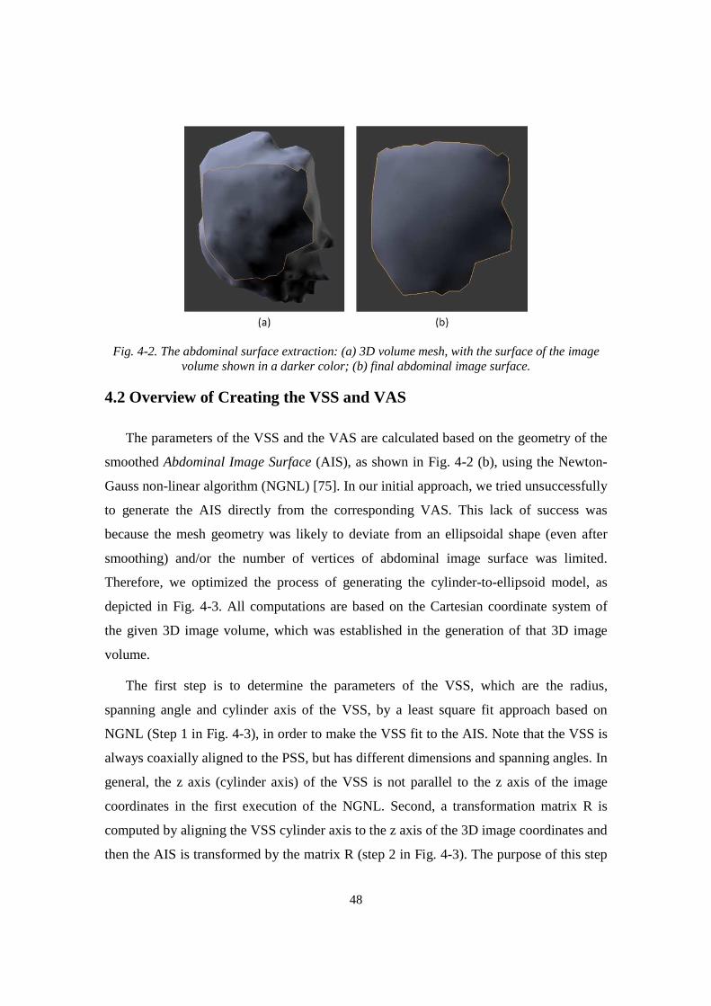
48

Fig. 4-2. The abdominal surface extraction: (a) 3D volume mesh, with the surface of the image volume shown in a darker color; (b) final abdominal image surface.

4.2 Overview of Creating the VSS and VAS

The parameters of the VSS and the VAS are calculated based on the geometry of the

smoothed Abdominal Image Surface (AIS), as shown in Fig. 4-2 (b), using the Newton-

Gauss non-linear algorithm (NGNL) [75]. In our initial approach, we tried unsuccessfully

to generate the AIS directly from the corresponding VAS. This lack of success was

because the mesh geometry was likely to deviate from an ellipsoidal shape (even after

smoothing) and/or the number of vertices of abdominal image surface was limited.

Therefore, we optimized the process of generating the cylinder-to-ellipsoid model, as

depicted in Fig. 4-3. All computations are based on the Cartesian coordinate system of

the given 3D image volume, which was established in the generation of that 3D image

volume.

The first step is to determine the parameters of the VSS, which are the radius,

spanning angle and cylinder axis of the VSS, by a least square fit approach based on

NGNL (Step 1 in Fig. 4-3), in order to make the VSS fit to the AIS. Note that the VSS is

always coaxially aligned to the PSS, but has different dimensions and spanning angles. In

general, the z axis (cylinder axis) of the VSS is not parallel to the z axis of the image

coordinates in the first execution of the NGNL. Second, a transformation matrix R is

computed by aligning the VSS cylinder axis to the z axis of the 3D image coordinates and

then the AIS is transformed by the matrix R (step 2 in Fig. 4-3). The purpose of this step

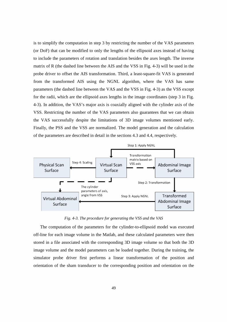
49

is to simplify the computation in step 3 by restricting the number of the VAS parameters

(or DoF) that can be modified to only the lengths of the ellipsoid axes instead of having

to include the parameters of rotation and translation besides the axes length. The inverse

matrix of R (the dashed line between the AIS and the VSS in Fig. 4-3) will be used in the

probe driver to offset the AIS transformation. Third, a least-square-fit VAS is generated

from the transformed AIS using the NGNL algorithm, where the VAS has same

parameters (the dashed line between the VAS and the VSS in Fig. 4-3) as the VSS except

for the radii, which are the ellipsoid axes lengths in the image coordinates (step 3 in Fig.

4-3). In addition, the VAS’s major axis is coaxially aligned with the cylinder axis of the

VSS. Restricting the number of the VAS parameters also guarantees that we can obtain

the VAS successfully despite the limitations of 3D image volumes mentioned early.

Finally, the PSS and the VSS are normalized. The model generation and the calculation

of the parameters are described in detail in the sections 4.3 and 4.4, respectively.

Fig. 4-3. The procedure for generating the VSS and the VAS

The computation of the parameters for the cylinder-to-ellipsoid model was executed

off-line for each image volume in the Matlab, and these calculated parameters were then

stored in a file associated with the corresponding 3D image volume so that both the 3D

image volume and the model parameters can be loaded together. During the training, the

simulator probe driver first performs a linear transformation of the position and

orientation of the sham transducer to the corresponding position and orientation on the

50

VSS, followed by a second linear transformation in the probe driver to the VAS that

actually represents the abdominal surface of the image volume.

4.3 Generation of the VSS Model

The generations of the VSS and the VAS involve several coordinate systems,

including the world coordinate system, the physical scan surface coordinate system and

the 3D image volume coordinate system. Given that the VSS and VAS are directly

derived from the AIS of a given 3D image volume, all computations in this section are

based on the 3D image volume coordinate system.

An arbitrary point (xc, yc, zc) on the cylinder surface that computes the least-square-fit

VSS can be parametrically expressed in eq. (4-1):

TUV+VWVX = �� ∗ �� ∗ T( cos �( sin �Y X + TU�+�W�X (4-1)

where θ is a free variable (0 ≤ θ <2π) and L is the length of the cylinder (-∞ < L < ∞);

further, (x0, y0, z0) is a point on the axis of the cylinder; r is the cylinder radius; Rx and Ry

are rotation matrices derived from θx and θy that denote the rotation angles of the cylinder

axis around the x and y axes, respectively, as given in eq. (4-2) and (4-3). The parameters

of L, r, x0, y0, z0, θx and θy are fixed values for a specific cylinder. The matrix Rz, which

denotes the rotation around the z axis, is not included in eq. (4-1). This is because the

cylinder axis of the final VSS for a given AIS was roughly parallel to the z axis in our

early studies and Rz was not necessary to our following calculation.

�� = T1 0 00 �)1�� −1�!��0 1�!�� �)1�� X (4-2)

�� = Z �)1�� 0 1�!��0 1 0−1�!�� 0 �)1��[ (4-3)

Translating and/or rotating a cylinder to make it be the least-square-fit (LSF) to the

AIS is a challenging task. Instead, the cylinder is assumed to be in a fixed position and

the AIS is manipulated to obtain the VSS. The fixed cylinder is described in eq. (4-4).

51

TUV+VWVX = T( cos �( sin �1 X (4-4)

First, the AIS, which is described in terms of vertices and faces, is translated by a

vector vt = (0, 0, - zcent) as shown in eq. (4-5), where (vxi, vyi, vzi) and (v’xi, v’yi, v’zi)

represent ith initial and translated vertex of the AIS, respectively. N is the total number of

the AIS vertices. The variable zcent is obtained from the AIS centroid (xcent, ycent, zcent),

calculated in eq. (4-6).

Z\′�I\′�I\′I[ = T\�I\�I\IX - T00WV^_`X 1 ≤ � ≤ b (4-5)

TUV^_`+V^_`WV^_`X = cddde�f∑ \�IfIh��f∑ \�IfIh��f∑ \IfIh� ijj

jk 1 ≤ � ≤ b (4-6)

To use the NGNL, a five-parameter set s = (θx, θy, xt, yt, r) is defined to manage the

translation and rotation of the cylinder. The solution of eq. (4-7) gives the cylinder that is

least square fit to the corresponding AIS. Similar to (4-1), θ is a free variable (0 ≤ θ <2π);

L is the length of the cylinder; Rx and Ry are rotation matrices; r is the cylinder radius; (xt,

yt, 0) is a point on the axis of the cylinder.

TUV+VWVX = �� ∗ �� ∗ T( cos �( sin �Y X + lU`+0̀ m (4-7)

To solve eq. (4-7), the NGNL requires an initial guess. Our initial study suggests that

the cylinder axis of the AIS was roughly parallel to the z-axis of the 3D image volume

coordinates, so the initial guess is set as θx=θy=0, xt = -xcent, yt = -ycent , r = c, where c is

constant number and associated with each 3D image volume. A vector d is defined such

that the i th scalar is the distance of ith vertex on the abdominal surface to the cylinder axis;

hence, this vector can be written as:

Z��I��I�I[ = �′� ∗ �′� ∗ nZ\′�I\′�I\′I[ − lU`+0̀ mo 1 ≤ � ≤ b (4-8)

52

where dxi, dyi, dzi are the i th distance that is projected to the x, y and z axes. R’x and R’y are

inverse matrices of Rx, Ry. The distance of a vertex to the cylinder surface is:

pI = q��I ��I �Ir ∗ b� − ( (4-9)

,ℎ3(3b� = cdddddde ��Is��I� + ��I���Is��I� + ��I�0 ijj

jjjjk 1 ≤ � ≤ b

To minimize the f = [f 1, f2,…, fN], a Jacobian Matrix is constructed in eq. (4-10).

t = u vwJvxJ vwJvxL vwJvxN⋯ ⋯ ⋯vwzvxJ vwzvxL vwzvxNvwJvx{⋯vwzvx{

vwJvx|⋯vwzvx|} (4-10)

where

455555565555557�pI�1� = b� ∗ �′� ∗ ��′� ∗ nZ\′�I\′�I\′I[ − lU`+0̀ mo�pI�1� = b� ∗ ��′� ∗ �′� ∗ nZ\′�I\′�I\′I[ − lU`+0̀ mo�pI�1� = b� ∗ �′� ∗ �′� ∗ T−100 X

�pI�1� = b� ∗ �′� ∗ �′� ∗ T 0−10 X�pI�1� = −1

1 ≤ � ≤ b

dR’x, dR’y are the derivatives of R’x, R’y.

��′� = T1 0 00 −1�!�� −�)1��0 �)1�� −1�!��X (4-11)

��′� = Z−1�!�� 0 �)1��0 1 0−�)1�� 0 −1�!��[ (4-12)

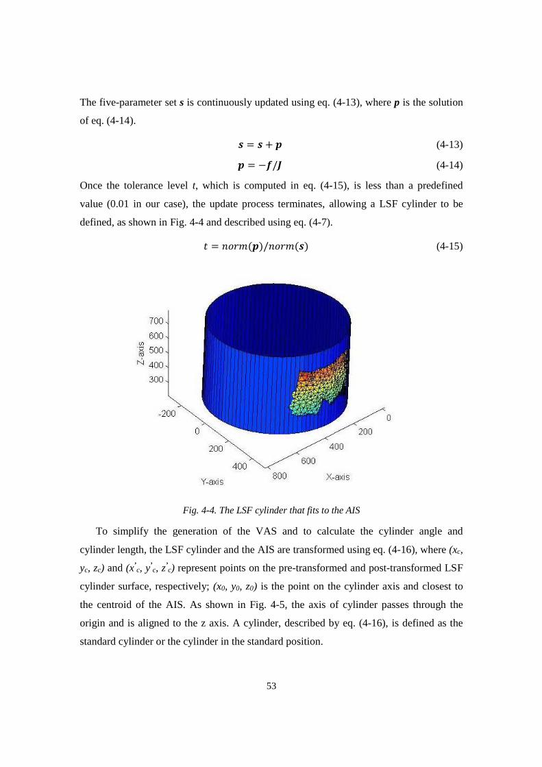
53

The five-parameter set s is continuously updated using eq. (4-13), where p is the solution

of eq. (4-14).

� = � + � (4-13)

� = −�/t (4-14)

Once the tolerance level t, which is computed in eq. (4-15), is less than a predefined

value (0.01 in our case), the update process terminates, allowing a LSF cylinder to be

defined, as shown in Fig. 4-4 and described using eq. (4-7).

� = !)(�(�)/!)(�(�) (4-15)

Fig. 4-4. The LSF cylinder that fits to the AIS

To simplify the generation of the VAS and to calculate the cylinder angle and

cylinder length, the LSF cylinder and the AIS are transformed using eq. (4-16), where (xc,

yc, zc) and (x’c, y’

c, z’c) represent points on the pre-transformed and post-transformed LSF

cylinder surface, respectively; (x0, y0, z0) is the point on the cylinder axis and closest to

the centroid of the AIS. As shown in Fig. 4-5, the axis of cylinder passes through the

origin and is aligned to the z axis. A cylinder, described by eq. (4-16), is defined as the

standard cylinder or the cylinder in the standard position.

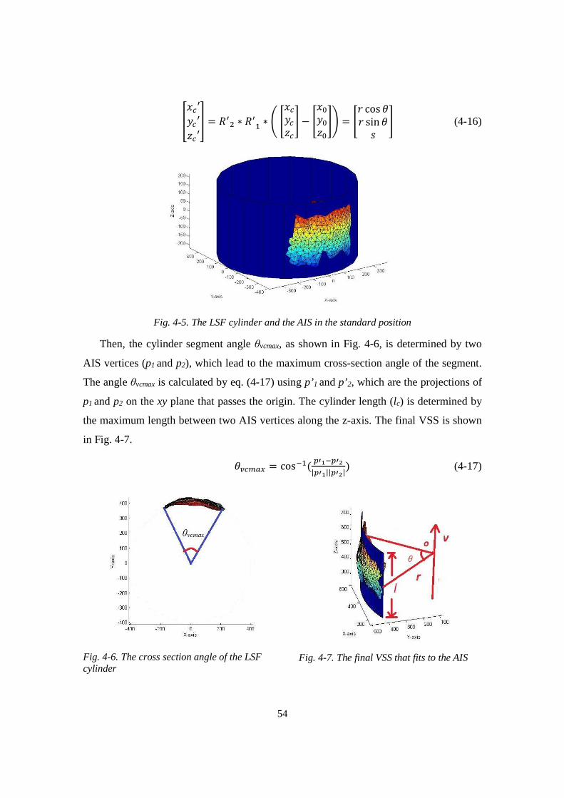
54

ZUV′+V′WV′[ = ��� ∗ ��� ∗ �TUV+VWVX − TU�+�W�X� = T( cos �( sin �1 X (4-16)

Fig. 4-5. The LSF cylinder and the AIS in the standard position

Then, the cylinder segment angle θvcmax, as shown in Fig. 4-6, is determined by two

AIS vertices (p1 and p2), which lead to the maximum cross-section angle of the segment.

The angle θvcmax is calculated by eq. (4-17) using p’1 and p’2, which are the projections of

p1 and p2 on the xy plane that passes the origin. The cylinder length (lc) is determined by

the maximum length between two AIS vertices along the z-axis. The final VSS is shown

in Fig. 4-7.

��V��� = cosF�( ��JF��L|��J||��L|) (4-17)

Fig. 4-6. The cross section angle of the LSF cylinder

Fig. 4-7. The final VSS that fits to the AIS

55

4.4 Generation of the VAS Model

Similar to the generation of the VSS, an ellipsoid that is a least square fit to the

transformed AIS can be simply expressed using eq. (4-18), where a, b and c are the radii

of the ellipsoid along the x, y and z axes, 0 ≤ φ <π, 0 ≤ θ <2π. Thus, a parameter set s =

(a,b,c) can be used to manipulate the geometry of ellipsoid.

TU^+̂W^X = T cos � sin �� sin � sin�� cos � X (4-18)

An N-by-3 matrix f is defined, whose ith row vector is the minimized distance from

the ith vertex (vxi, vyi, vzi) of the AIS to a point (xei, yei, zei) on the ellipsoid surface:

�� = ZpI�pI�pI�[ ′ = �T\�I\�I\IX − TU^I+^IW^IX� ′ (4-19)

To minimize the matrix f, another Jacobian matrix is constructed, as shown in

equation (3-20). N is the total number of the AIS vertices.

t = u vwJvxJ vwJvxL vwJvxN⋯ ⋯ ⋯vwzvxJ vwzvxL vwzvxN} (4-20)

where455565557�pI�1� = T−cos � sin�00 X�pI�1� = T 0−sin � sin�0 X�pI�1� = T 00− cos �X

1 ≤ � ≤ b

The parameter set s is continuously updated using eq. (4-13) and (4-14) until the

tolerance value reaches a predefined value (0.01 in our case). The initial guess of the

ellipsoid radii are set to half of the AIS lengths along x, y and z axes. The LSF ellipsoid

and the final VAS are shown in Fig. 4-8 and Fig. 4-9, respectively. The VAS length along

z-axis is equal to the VSS length.

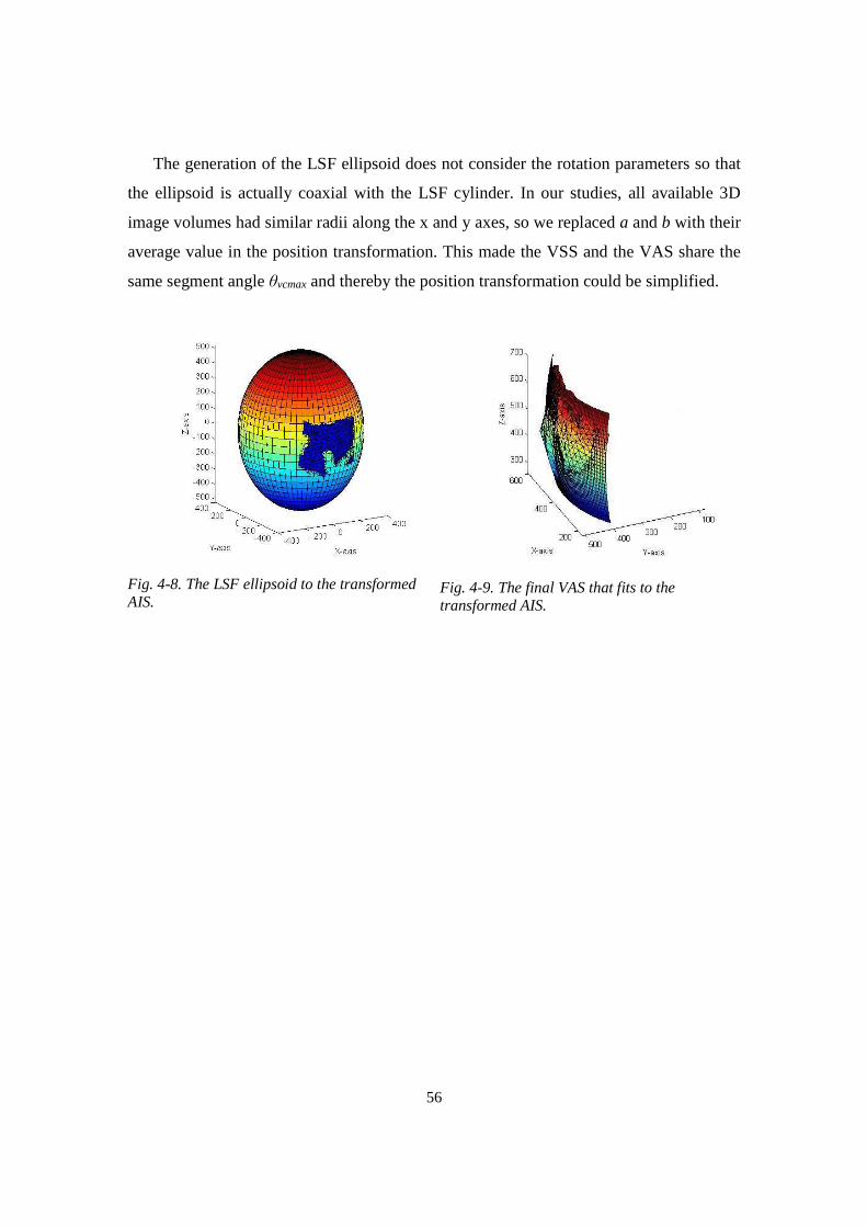
56

The generation of the LSF ellipsoid does not consider the rotation parameters so that

the ellipsoid is actually coaxial with the LSF cylinder. In our studies, all available 3D

image volumes had similar radii along the x and y axes, so we replaced a and b with their

average value in the position transformation. This made the VSS and the VAS share the

same segment angle θvcmax and thereby the position transformation could be simplified.

Fig. 4-8. The LSF ellipsoid to the transformed AIS.

Fig. 4-9. The final VAS that fits to the transformed AIS.

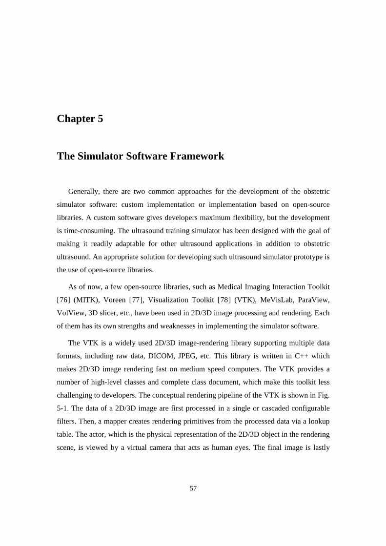
57

Chapter 5

The Simulator Software Framework

Generally, there are two common approaches for the development of the obstetric

simulator software: custom implementation or implementation based on open-source

libraries. A custom software gives developers maximum flexibility, but the development

is time-consuming. The ultrasound training simulator has been designed with the goal of

making it readily adaptable for other ultrasound applications in addition to obstetric

ultrasound. An appropriate solution for developing such ultrasound simulator prototype is

the use of open-source libraries.

As of now, a few open-source libraries, such as Medical Imaging Interaction Toolkit

[76] (MITK), Voreen [77], Visualization Toolkit [78] (VTK), MeVisLab, ParaView,

VolView, 3D slicer, etc., have been used in 2D/3D image processing and rendering. Each

of them has its own strengths and weaknesses in implementing the simulator software.

The VTK is a widely used 2D/3D image-rendering library supporting multiple data

formats, including raw data, DICOM, JPEG, etc. This library is written in C++ which

makes 2D/3D image rendering fast on medium speed computers. The VTK provides a

number of high-level classes and complete class document, which make this toolkit less

challenging to developers. The conceptual rendering pipeline of the VTK is shown in Fig.

5-1. The data of a 2D/3D image are first processed in a single or cascaded configurable

filters. Then, a mapper creates rendering primitives from the processed data via a lookup

table. The actor, which is the physical representation of the 2D/3D object in the rendering

scene, is viewed by a virtual camera that acts as human eyes. The final image is lastly

58

displayed in a VTK rendering window. Although the VTK offers powerful visualization,

only limited number of User Interface (UI) classes are provided to developers.

Fig. 5-1. The VTK data flow.

The Voreen is an interactive visualization framework written in C++. It provides a

prototyping environment where a user is able to visually create the data processing and

rendering pipeline without coding. This feature, visualized programming, allows the

developer to drag, connect and configure a set of processors, which contain a number of

built-in functions, without touching low-level classes. For the developers who have

limited programming experience, the visualized programming eases their work in

processing and rendering 2D/3D data. However, the visual programming approach

sacrifices the flexibility of an open source library and is less useful for implementing our

obstetric ultrasound simulator. Similar to the VTK, the Voreen supports multiple medical

data formats, such as TIFF, RAW, and DICOM. Another feature of the Voreen is the

GPU-based ray-casting technique. This feature, however, restricts this toolkit to the

platforms having NVIDIA and ATI graphic cards installed because the high

computational demands resulting from the ray-casting technique has to be computed on a

GPU.

The MeVisLab is another visual programming toolkit, which only allows limited

custom codes to be added to a new application. This restriction actually makes the

development of our simulator impossible on the MeVisLab. Another limitation of the

MeVisLab is that the toolkit is implemented with the object-oriented (OO) programming.

The MeVisLab utilizes the underlying library, the OpenGL, to complete the rendering, in

which the OpenGL needs to globally access the rendering data. The OO design principle

59

requires the data to be encapsulated into an instance and thus make graphics performance

less efficient.

The VolView and the ParaView are two open source 3D rendering libraries based on

the VTK. Both of them require the developer to purchase support service from Kitware to

receive technical supports and development training. This would pose a budget challenge

to our academic research. Moreover, the VolView only supports 3D volume data and

thereby it is not suitable for implementing our simulator, which needs to process 2D

images and mesh data.

The MITK, a superset of the Insight Toolkit (ITK) and the VTK, creates a single

rendering pipeline so that the ITK’s image processing algorithms can be seamlessly

integrated into the VTK rendering process. The MITK not only inherits all classes from

the ITK and the VTK but also extends them by providing easy-to-use UI classes. In

addition to the common medical data formats supported by the above open source

libraries, the MITK is able to handle non-medical data. The feature of being independent

from a graphic UI library makes it available to be integrated into multiple application

frameworks besides the current Qt platform.

One critical consideration in the simulator design is that the system must guarantee

smooth visual experience by being able to render more than 25 frames (2D images) per

second on a typical recent computer. Given that the ray-casting technology has problems

in the rendering speed and precision [79], we have chosen the MITK as our development

platform. For the UI design, we use the Qt [80], which is a widely used cross-platform

application framework. The MITK has implemented a few Qt widgets that can quickly

bind the image processing and the rendering libraries to the simulator.

5.1 Overview of Qt and MITK

5.1.1 Overview of the Qt framework

The first version of the Qt toolkit was released in 1995. It was initially developed by

Trolltech, which later was purchased by Nokia. The Qt is currently being developed by

the Digia and is available to developers through a commercial license or an open source

license. There are two major Qt versions that have been widely used by developers, the

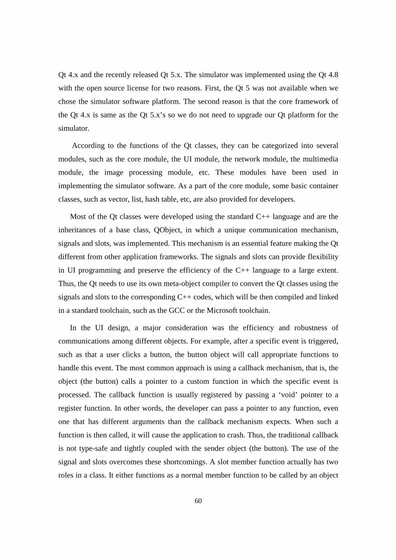
60

Qt 4.x and the recently released Qt 5.x. The simulator was implemented using the Qt 4.8

with the open source license for two reasons. First, the Qt 5 was not available when we

chose the simulator software platform. The second reason is that the core framework of

the Qt 4.x is same as the Qt 5.x’s so we do not need to upgrade our Qt platform for the

simulator.

According to the functions of the Qt classes, they can be categorized into several

modules, such as the core module, the UI module, the network module, the multimedia

module, the image processing module, etc. These modules have been used in

implementing the simulator software. As a part of the core module, some basic container

classes, such as vector, list, hash table, etc, are also provided for developers.

Most of the Qt classes were developed using the standard C++ language and are the

inheritances of a base class, QObject, in which a unique communication mechanism,

signals and slots, was implemented. This mechanism is an essential feature making the Qt

different from other application frameworks. The signals and slots can provide flexibility

in UI programming and preserve the efficiency of the C++ language to a large extent.

Thus, the Qt needs to use its own meta-object compiler to convert the Qt classes using the

signals and slots to the corresponding C++ codes, which will be then compiled and linked

in a standard toolchain, such as the GCC or the Microsoft toolchain.

In the UI design, a major consideration was the efficiency and robustness of

communications among different objects. For example, after a specific event is triggered,

such as that a user clicks a button, the button object will call appropriate functions to

handle this event. The most common approach is using a callback mechanism, that is, the

object (the button) calls a pointer to a custom function in which the specific event is

processed. The callback function is usually registered by passing a ‘void’ pointer to a

register function. In other words, the developer can pass a pointer to any function, even

one that has different arguments than the callback mechanism expects. When such a

function is then called, it will cause the application to crash. Thus, the traditional callback

is not type-safe and tightly coupled with the sender object (the button). The use of the

signal and slots overcomes these shortcomings. A slot member function actually has two

roles in a class. It either functions as a normal member function to be called by an object

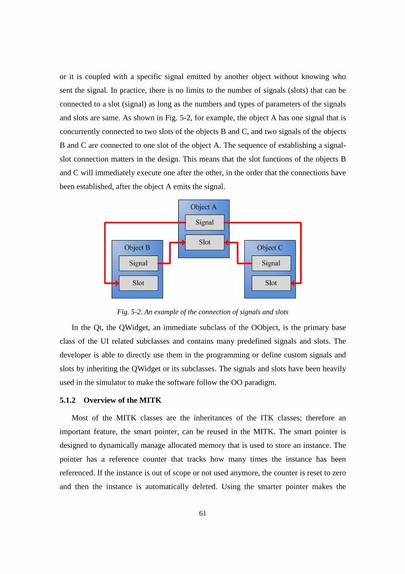
61

or it is coupled with a specific signal emitted by another object without knowing who

sent the signal. In practice, there is no limits to the number of signals (slots) that can be

connected to a slot (signal) as long as the numbers and types of parameters of the signals

and slots are same. As shown in Fig. 5-2, for example, the object A has one signal that is

concurrently connected to two slots of the objects B and C, and two signals of the objects

B and C are connected to one slot of the object A. The sequence of establishing a signal-

slot connection matters in the design. This means that the slot functions of the objects B

and C will immediately execute one after the other, in the order that the connections have

been established, after the object A emits the signal.

Fig. 5-2. An example of the connection of signals and slots

In the Qt, the QWidget, an immediate subclass of the OObject, is the primary base

class of the UI related subclasses and contains many predefined signals and slots. The

developer is able to directly use them in the programming or define custom signals and

slots by inheriting the QWidget or its subclasses. The signals and slots have been heavily

used in the simulator to make the software follow the OO paradigm.

5.1.2 Overview of the MITK

Most of the MITK classes are the inheritances of the ITK classes; therefore an

important feature, the smart pointer, can be reused in the MITK. The smart pointer is

designed to dynamically manage allocated memory that is used to store an instance. The

pointer has a reference counter that tracks how many times the instance has been

referenced. If the instance is out of scope or not used anymore, the counter is reset to zero

and then the instance is automatically deleted. Using the smarter pointer makes the

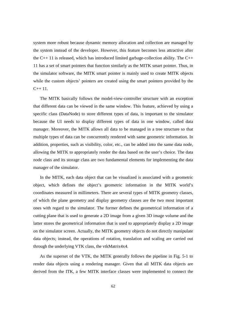
62

system more robust because dynamic memory allocation and collection are managed by

the system instead of the developer. However, this feature becomes less attractive after

the C++ 11 is released, which has introduced limited garbage-collection ability. The C++

11 has a set of smart pointers that function similarly as the MITK smart pointer. Thus, in

the simulator software, the MITK smart pointer is mainly used to create MITK objects

while the custom objects’ pointers are created using the smart pointers provided by the

C++ 11.

The MITK basically follows the model-view-controller structure with an exception

that different data can be viewed in the same window. This feature, achieved by using a

specific class (DataNode) to store different types of data, is important to the simulator

because the UI needs to display different types of data in one window, called data

manager. Moreover, the MITK allows all data to be managed in a tree structure so that

multiple types of data can be concurrently rendered with same geometric information. In

addition, properties, such as visibility, color, etc., can be added into the same data node,

allowing the MITK to appropriately render the data based on the user’s choice. The data

node class and its storage class are two fundamental elements for implementing the data

manager of the simulator.

In the MITK, each data object that can be visualized is associated with a geometric

object, which defines the object’s geometric information in the MITK world’s

coordinates measured in millimeters. There are several types of MITK geometry classes,

of which the plane geometry and display geometry classes are the two most important

ones with regard to the simulator. The former defines the geometrical information of a

cutting plane that is used to generate a 2D image from a given 3D image volume and the

latter stores the geometrical information that is used to appropriately display a 2D image

on the simulator screen. Actually, the MITK geometry objects do not directly manipulate

data objects; instead, the operations of rotation, translation and scaling are carried out

through the underlying VTK class, the vtkMatrix4x4.

As the superset of the VTK, the MITK generally follows the pipeline in Fig. 5-1 to

render data objects using a rendering manager. Given that all MITK data objects are

derived from the ITK, a few MITK interface classes were implemented to connect the

63

ITK-derived objects to the VTK pipeline, as shown in Fig. 5-3. After the update

procedure is initiated by the rendering manager, a MITK rendering window, derived from

the QVTK Widget, sends the request to its corresponding VTK renderer through an

associated MITK renderer. Then, the VTK renderer manipulates the corresponding VTK

actors and then completes the rest of rendering procedure. Thus, the MITK rendering

window is able to directly display the final image without involving additional data type

conversion. The VTK actor, actually rendered by the VTK, are indirectly managed by the

MITK renderer through a specific interface class, the vtkMiktRenderProp class. In

practice, the MITK renderer acts as a delegator of the VTK renderer to indirectly

participate in the rendering procedure.

Fig. 5-3. Data rendering in the MITK.

5.2 Overview of the Simulator Software

The simulator software contains several components, or blocks, as shown in Fig. 5-4,

including the UI, the virtual reality module, the data manager, the sham transducer driver,

the 2D image reslicer, the training assessment and the communication module. The

simulator UI is responsible for interacting with the user and managing the communication

among the software blocks. The communication block, as an essential part of the remote

training system, will be described in Chapter 8. The automatic training assessment will be

detailed in Chapter 6.

Before the UI and other software components are described, we will introduce

another concept, the anatomical landmark, which represents an anatomical structure

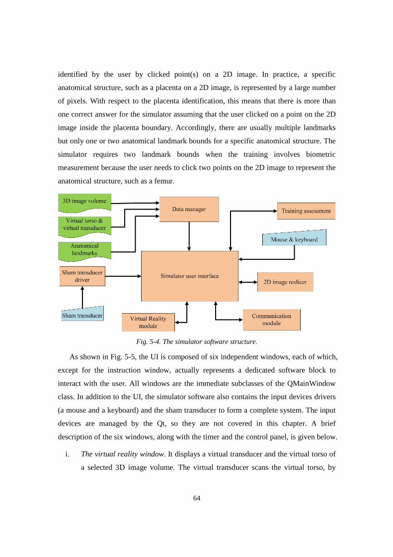
64

identified by the user by clicked point(s) on a 2D image. In practice, a specific

anatomical structure, such as a placenta on a 2D image, is represented by a large number

of pixels. With respect to the placenta identification, this means that there is more than

one correct answer for the simulator assuming that the user clicked on a point on the 2D

image inside the placenta boundary. Accordingly, there are usually multiple landmarks

but only one or two anatomical landmark bounds for a specific anatomical structure. The

simulator requires two landmark bounds when the training involves biometric

measurement because the user needs to click two points on the 2D image to represent the

anatomical structure, such as a femur.

Fig. 5-4. The simulator software structure.

As shown in Fig. 5-5, the UI is composed of six independent windows, each of which,

except for the instruction window, actually represents a dedicated software block to

interact with the user. All windows are the immediate subclasses of the QMainWindow

class. In addition to the UI, the simulator software also contains the input devices drivers

(a mouse and a keyboard) and the sham transducer to form a complete system. The input

devices are managed by the Qt, so they are not covered in this chapter. A brief

description of the six windows, along with the timer and the control panel, is given below.

i. The virtual reality window. It displays a virtual transducer and the virtual torso of

a selected 3D image volume. The virtual transducer scans the virtual torso, by

65

exactly following the movements of the sham transducer. A scan path is also

displayed on the virtual torso in the form of white dots.

ii. The data manager window. It shows a selected 3D image volume and the

anatomical landmarks identified/measured by the user. The user is also able to

review the 2D image that contains the landmark(s) identified in the previous tasks

or to delete the landmark(s) identified by mistake.

iii. The 2D image rendering window. A 2D ultrasound image, extracted from a

selected image volume, is displayed in this window. Meanwhile, it interacts with

the user by allowing him or her to click maternal and fetal organs and tissues on

the 2D image with a mouse.

iv. The instruction window. It displays the instructions of a given training task as well

as the evaluation feedback provided by the simulator.

v. The landmark window. It has two drop-down menus. The upper one is used for

choosing the name of the anatomical structure that the user is identifying. The

lower one is used for reviewing a biometric measurement value.

vi. The timer. The simulator informs the user of the total time he or she has spent on

a selected training image and tracks the scan time of each task. This timer is reset

to zero when an image volume is loaded into the simulator.

vii. The ultrasound console window. The user configures the scan depth, the overall

gain, and the transducer type.

viii. The control panel. The buttons on this panel was designed to make the user easily

move from a given task to the previous or next task or repeat this task. After the

button ‘repeat task’ is pressed, the simulator automatically resets the instruction

window and deletes all landmarks that have been identified by the user in this task.

The button ‘Clear Scan Path’ is used for removing the scan path shown on the

virtual torso.

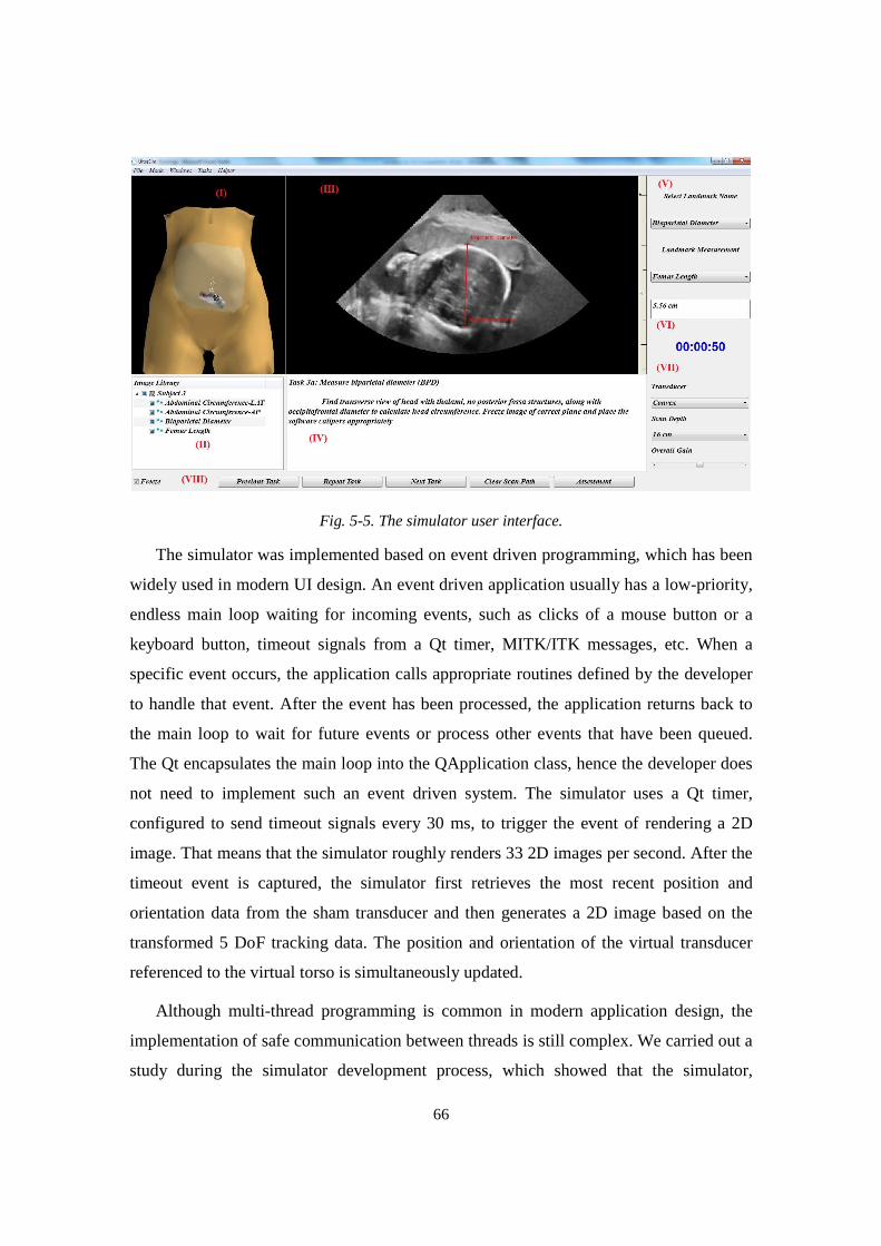
66

Fig. 5-5. The simulator user interface.

The simulator was implemented based on event driven programming, which has been

widely used in modern UI design. An event driven application usually has a low-priority,

endless main loop waiting for incoming events, such as clicks of a mouse button or a

keyboard button, timeout signals from a Qt timer, MITK/ITK messages, etc. When a

specific event occurs, the application calls appropriate routines defined by the developer

to handle that event. After the event has been processed, the application returns back to

the main loop to wait for future events or process other events that have been queued.

The Qt encapsulates the main loop into the QApplication class, hence the developer does

not need to implement such an event driven system. The simulator uses a Qt timer,

configured to send timeout signals every 30 ms, to trigger the event of rendering a 2D

image. That means that the simulator roughly renders 33 2D images per second. After the

timeout event is captured, the simulator first retrieves the most recent position and

orientation data from the sham transducer and then generates a 2D image based on the

transformed 5 DoF tracking data. The position and orientation of the virtual transducer

referenced to the virtual torso is simultaneously updated.

Although multi-thread programming is common in modern application design, the

implementation of safe communication between threads is still complex. We carried out a

study during the simulator development process, which showed that the simulator,

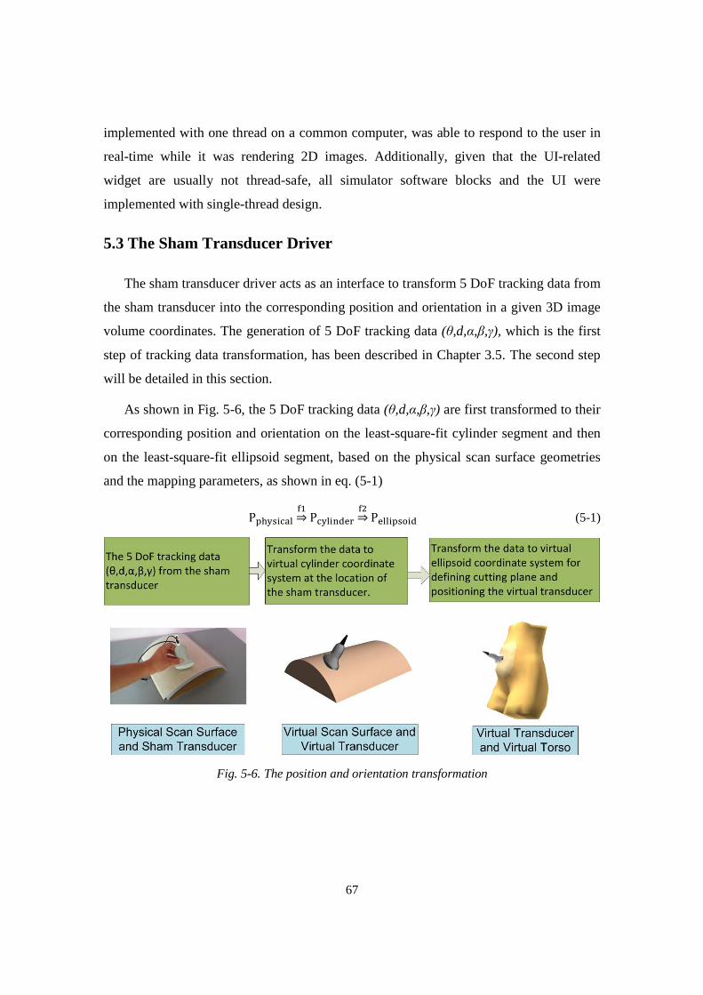
67

implemented with one thread on a common computer, was able to respond to the user in

real-time while it was rendering 2D images. Additionally, given that the UI-related

widget are usually not thread-safe, all simulator software blocks and the UI were

implemented with single-thread design.

5.3 The Sham Transducer Driver

The sham transducer driver acts as an interface to transform 5 DoF tracking data from

the sham transducer into the corresponding position and orientation in a given 3D image

volume coordinates. The generation of 5 DoF tracking data (θ,d,α,β,γ), which is the first

step of tracking data transformation, has been described in Chapter 3.5. The second step

will be detailed in this section.

As shown in Fig. 5-6, the 5 DoF tracking data (θ,d,α,β,γ) are first transformed to their

corresponding position and orientation on the least-square-fit cylinder segment and then

on the least-square-fit ellipsoid segment, based on the physical scan surface geometries

and the mapping parameters, as shown in eq. (5-1)

P�������� ��⇒ P�������� ��⇒P������ �� (5-1)

Fig. 5-6. The position and orientation transformation

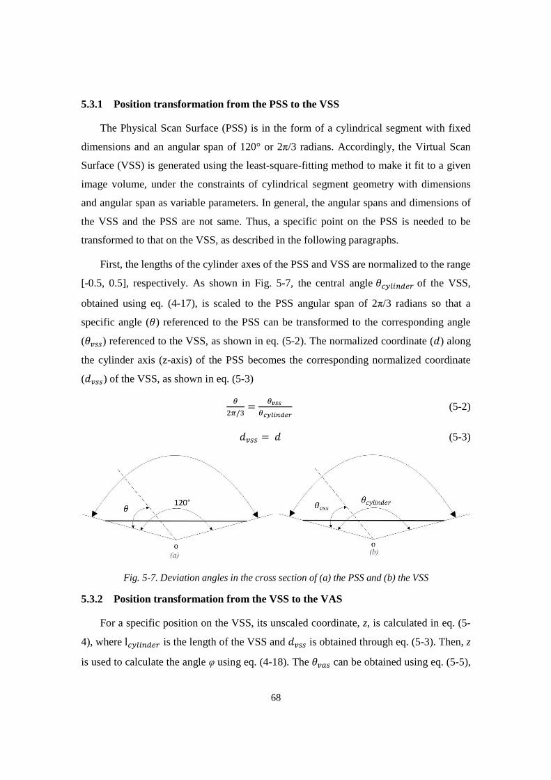
68

5.3.1 Position transformation from the PSS to the VSS

The Physical Scan Surface (PSS) is in the form of a cylindrical segment with fixed

dimensions and an angular span of 120° or 2π/3 radians. Accordingly, the Virtual Scan

Surface (VSS) is generated using the least-square-fitting method to make it fit to a given

image volume, under the constraints of cylindrical segment geometry with dimensions

and angular span as variable parameters. In general, the angular spans and dimensions of

the VSS and the PSS are not same. Thus, a specific point on the PSS is needed to be

transformed to that on the VSS, as described in the following paragraphs.

First, the lengths of the cylinder axes of the PSS and VSS are normalized to the range

[-0.5, 0.5], respectively. As shown in Fig. 5-7, the central angle �V��I_¡^¢ of the VSS,

obtained using eq. (4-17), is scaled to the PSS angular span of 2π/3 radians so that a

specific angle (�) referenced to the PSS can be transformed to the corresponding angle

(��xx) referenced to the VSS, as shown in eq. (5-2). The normalized coordinate (�) along

the cylinder axis (z-axis) of the PSS becomes the corresponding normalized coordinate

(��xx) of the VSS, as shown in eq. (5-3)

Q��/� = Q£¤¤ Q¥¦§¨©ª«¬ (5-2)

��xx = � (5-3)

Fig. 5-7. Deviation angles in the cross section of (a) the PSS and (b) the VSS

5.3.2 Position transformation from the VSS to the VAS

For a specific position on the VSS, its unscaled coordinate, z, is calculated in eq. (5-

4), where lV��I_¡^¢ is the length of the VSS and ��xx is obtained through eq. (5-3). Then, z

is used to calculate the angle φ using eq. (4-18). The ���x can be obtained using eq. (5-5),

69

where the VAS refers to the Virtual Abdominal Surface (VAS), and then plugged into eq.

(4-18) to calculate the x and y coordinates. All above position transformations are

actually referenced to the 3D image volume coordinates, so the (x, y, z) is the final

position for guiding 2D ultrasound image extraction.

W = lV��I_¡^¢ ∙ ��xx (5-4)

���x = ��xx (5-5)

5.3.3 Orientation transformation

The orientation data from the IMU are referenced to world coordinates, defined by

the gravity and magnetic north vectors, and need to be transformed to the corresponding

orientation in the PSS coordinates and then in the local coordinates established at the

scanning point, that is, the contact point of the sham transducer on the PSS, as shown in

eq. (5-6), based on the geometries of the VSS and the VAS, respectively. The

transformed orientation data will be used by the 2D image slicer to generate the

corresponding image. The transformed orientation data, which actually represent the

Euler angles that forms a rotation matrix, are used to determine the cutting plane’s

orientation in the 3D image coordinates.

Q® ��� ��⇒ Q¯°° ��⇒Q� ��� (5-6)

The orientation transformation involves the quaternion multiplication and the

conversion between Euler angles and a quaternion. This is because the transformation can

only be linearly calculated based on the quaternion whereas we are only able to obtain the

transducer’s rotation in the form of Euler angles in the PSS coordinates. We assume that D is the quaternion derived from the (α,β,γ); therefore D can be expressed by the

multiplication of two quaternions D� and D�, as shown in eq. (5-7). D� denotes that the

sham transducer only rotates around the z axis of the PSS starting from the identity

quaternion (Fig. 3-8) in the PSS coordinates. D� is the rotation referenced to the local

coordinates established at the contact point on the PSS, as shown in Fig. 3-9.

D = D� ∗ D� (5-7)

70

The orientation referenced to the VSS is then obtained by multiplying D� with the

inverse quaternion of D� and with a quaternion D�� , as shown in eq. (5-8). D�� is derived

from the deviation angle ��xx in Fig. 5-7.

D�xx = D� ∙ D� ∙ D�F� ∙ D�� (5-8)

As shown in Fig. 5-7 and eq. (5-5), the deviation angle (��xx) on the VSS is same as

the deviation angle (���x) on the VAS, so we can directly use the quaternion D�xx as the

final quaternion, which is referenced to the 3D image volume coordinates.

5.4 The Virtual Torso and the Virtual Transducer

The PSS, a cylindrical segment with fixed dimensions, simulating the human

abdomen, provides only a generic representation of the actual abdominal surface of a

pregnant woman who was scanned to acquire the 3D image volume. Given that the

geometry of a pregnant woman’s abdomen slightly varies from person to person, we

utilized virtual reality to enhance the simulator realism. While the user is performing

ultrasound scan with the sham transducer, a virtual transducer scans the virtual torso of a

selected 3D image volume by following the movements of the sham transducer on the

PSS with respect to both position and orientation. Thus, the limitation in realism caused

by using the generic physical scan surface can be alleviated by using the virtual torso,

whose abdominal surface is geometrically in proportion to the selected 3D image’s

abdominal surface.

We implemented the virtual torso by manually blending a generic female body with

the unique abdominal image surface (the AIS) of a given 3D image volume in Blender

software, as shown in Fig. 5-8. First, the AIS is generated as described in Chapter 4.1.

Then, the AIS is scaled down so that all of its vertices coordinates are in the range of (-1,

1) using the following equations. We assume (UI , +I , WI) and (UI�, +I�, WI�) are the

coordinates of the �`± vertex of the original AIS and the scaled AIS, respectively.

²�� = (U�I_ +U���)/2�� = (+�I_ ++���)/2� = (W�I_ +W³�´)/2 (5-9)

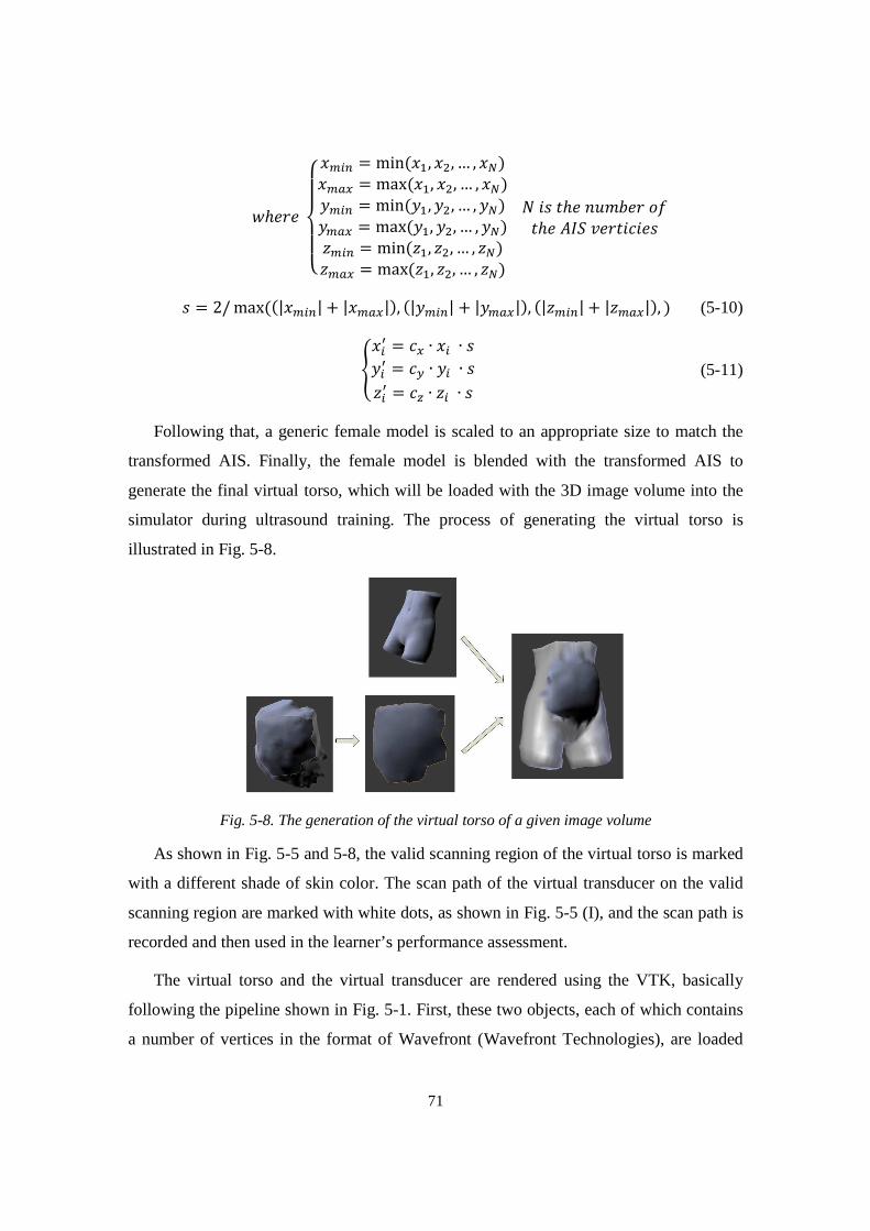
71

,ℎ3(345657U�I_ = min(U�, U�, … , Uf)U��� = max(U�, U�, … , Uf)+�I_ = min(+�, +�, … , +f)+��� = max(+�, +�, … , +f)W�I_ = min(W�, W�, … , Wf)W��� = max(W�, W�, … , Wf)

b�1�ℎ3!¸��3()p�ℎ3¹º»\3(����31

1 = 2/max((|U�I_| + |U���|), (|+�I_| + |+���|), (|W�I_| + |W���|), ) (5-10)

²UI� = �� ∙ UI ∙ 1+I� = �� ∙ +I ∙ 1WI� = � ∙ WI ∙ 1 (5-11)

Following that, a generic female model is scaled to an appropriate size to match the

transformed AIS. Finally, the female model is blended with the transformed AIS to

generate the final virtual torso, which will be loaded with the 3D image volume into the

simulator during ultrasound training. The process of generating the virtual torso is

illustrated in Fig. 5-8.

Fig. 5-8. The generation of the virtual torso of a given image volume

As shown in Fig. 5-5 and 5-8, the valid scanning region of the virtual torso is marked

with a different shade of skin color. The scan path of the virtual transducer on the valid

scanning region are marked with white dots, as shown in Fig. 5-5 (I), and the scan path is

recorded and then used in the learner’s performance assessment.

The virtual torso and the virtual transducer are rendered using the VTK, basically

following the pipeline shown in Fig. 5-1. First, these two objects, each of which contains

a number of vertices in the format of Wavefront (Wavefront Technologies), are loaded

72

into the simulator by calling the VTK object reader class, vtkOBJReader. Their rendering

primitives, generated by the VTK map class, vtkMapper, form two entities, which are

also known as VTK actors, in the rendering scene. The VTK allows the developer to

configure the number, location and intensity of lights in the rendering scene to illuminate

the virtual torso. We utilized eight lights, positioned at the eight corners of the invisible

cube encompassing the virtual torso, in the simulator.

Although the cylinder-to-ellipsoid model had been used to optimize the

transformation of the tracking data, the virtual transducer failed to follow the virtual

abdominal surface at some locations, but instead either intersected or separated from the

virtual torso surface. To correct this problem, we have incorporated the SOftware Library

for Interference Detection (SOLID) into the simulator. As the core of the SOLID, the

simplex-based Gilbert-Johnson-Keerthi algorithm [ 81] is utilized to calculate the

Euclidean distance between two sets of vertices, which are exactly the basic elements of

the virtual transducer and the virtual torso. The collision detection starts with setting up

the position and orientation of the virtual transducer in the rendering scene based on the

transformed tracking data. Then, the distance function provided by the SOLID is called to

calculate the intersection depth or the distance of the virtual transducer to the virtual torso.

Finally, the calculated value is used to adjust the original position of the virtual

transducer.

5.5 The 2D Image Reslicer

This software block utilizes the transformed orientation and position to define a

cutting plane, which guides the extraction of a 2D slice (image) from a selected 3D image

volume. The generation of the 2D image is shown in Fig. 5-9. First, the coordinates of

every point on the cutting plane are transformed back to its corresponding coordinates,

(x,y,z), in the 3D image volume based on the tracking data from the sham transducer. If

all three coordinates (x,y,z) are valid integers (within the dimensions of the 3D image

volume), the intensity of the voxel at (x,y,z) is directly sampled. Otherwise, as is the case

under most circumstances, a tri-linear interpolation, explained in the next paragraph, is

used to calculate the intensity of the corresponding point based on its eight neighbor

voxels.

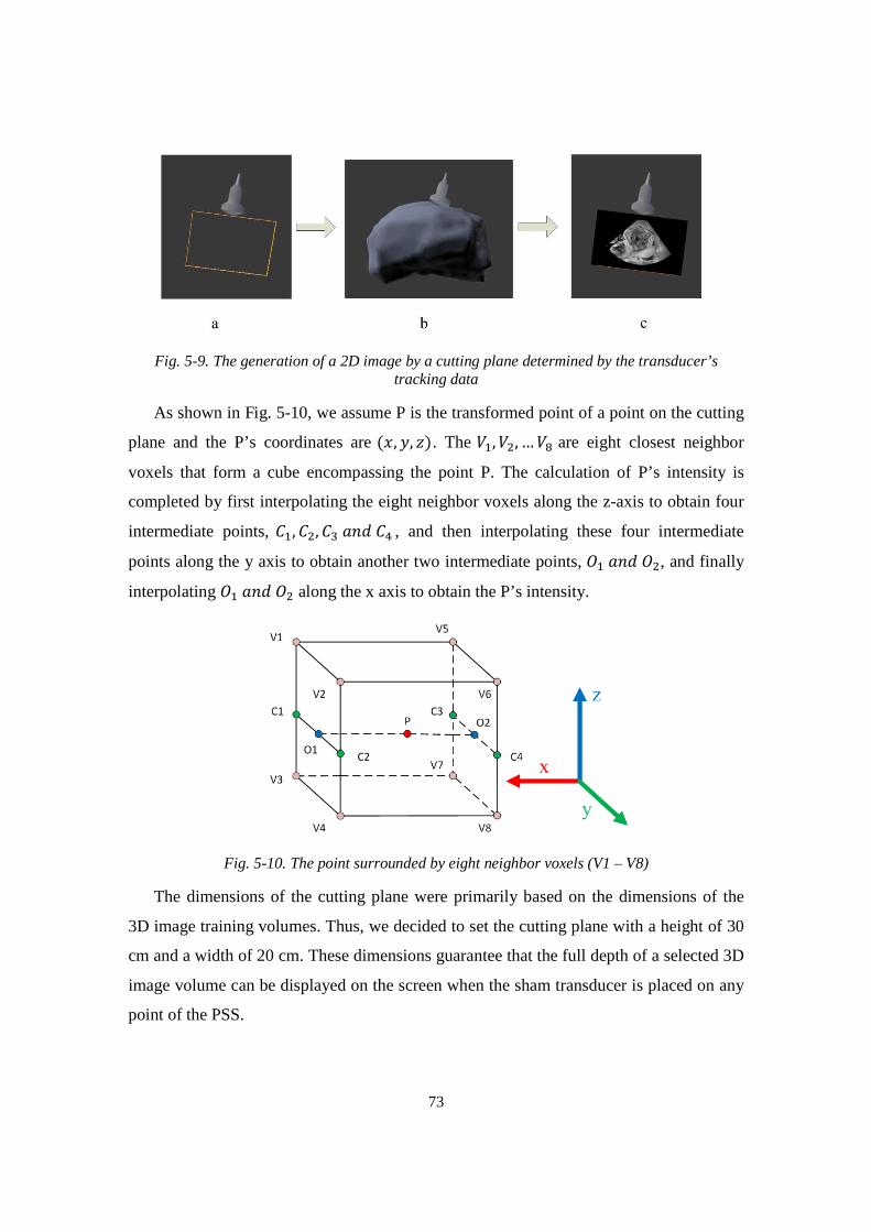
73

Fig. 5-9. The generation of a 2D image by a cutting plane determined by the transducer’s tracking data

As shown in Fig. 5-10, we assume P is the transformed point of a point on the cutting

plane and the P’s coordinates are (U, +, W). The ¼�, ¼�, …¼½ are eight closest neighbor

voxels that form a cube encompassing the point P. The calculation of P’s intensity is

completed by first interpolating the eight neighbor voxels along the z-axis to obtain four

intermediate points, ¾�, ¾�, ¾� !�¾� , and then interpolating these four intermediate

points along the y axis to obtain another two intermediate points, ¿� !�¿�, and finally

interpolating ¿� !�¿� along the x axis to obtain the P’s intensity.

Fig. 5-10. The point surrounded by eight neighbor voxels (V1 – V8)

The dimensions of the cutting plane were primarily based on the dimensions of the

3D image training volumes. Thus, we decided to set the cutting plane with a height of 30

cm and a width of 20 cm. These dimensions guarantee that the full depth of a selected 3D

image volume can be displayed on the screen when the sham transducer is placed on any

point of the PSS.

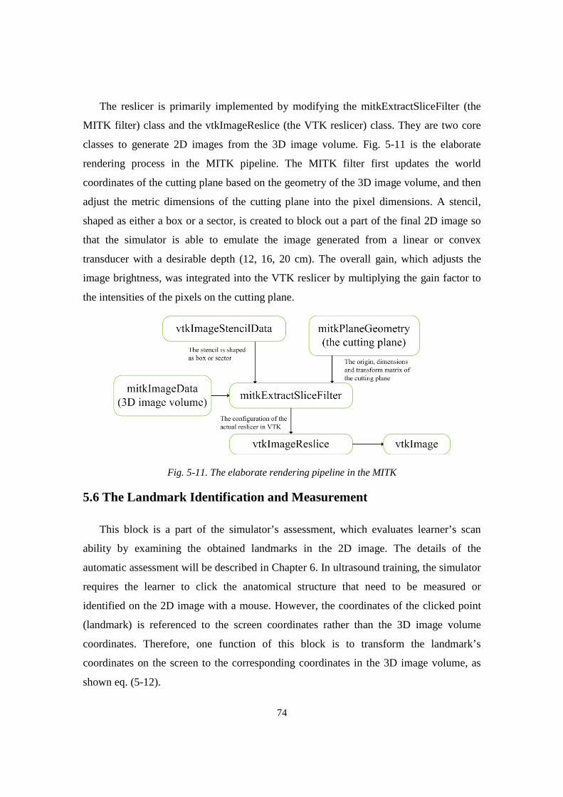
74

The reslicer is primarily implemented by modifying the mitkExtractSliceFilter (the

MITK filter) class and the vtkImageReslice (the VTK reslicer) class. They are two core

classes to generate 2D images from the 3D image volume. Fig. 5-11 is the elaborate

rendering process in the MITK pipeline. The MITK filter first updates the world

coordinates of the cutting plane based on the geometry of the 3D image volume, and then

adjust the metric dimensions of the cutting plane into the pixel dimensions. A stencil,

shaped as either a box or a sector, is created to block out a part of the final 2D image so

that the simulator is able to emulate the image generated from a linear or convex

transducer with a desirable depth (12, 16, 20 cm). The overall gain, which adjusts the

image brightness, was integrated into the VTK reslicer by multiplying the gain factor to

the intensities of the pixels on the cutting plane.

Fig. 5-11. The elaborate rendering pipeline in the MITK

5.6 The Landmark Identification and Measurement

This block is a part of the simulator’s assessment, which evaluates learner’s scan

ability by examining the obtained landmarks in the 2D image. The details of the

automatic assessment will be described in Chapter 6. In ultrasound training, the simulator

requires the learner to click the anatomical structure that need to be measured or

identified on the 2D image with a mouse. However, the coordinates of the clicked point

(landmark) is referenced to the screen coordinates rather than the 3D image volume

coordinates. Therefore, one function of this block is to transform the landmark’s

coordinates on the screen to the corresponding coordinates in the 3D image volume, as

shown eq. (5-12).

75

P������ À�⇒ P�Á����� À�⇒P�Á�³�Â� (5-12)

The screen coordinates are first transformed to the corresponding coordinates

referenced to the cutting plane, based on the dimensions of the screen image and the

cutting plane, and then to the coordinates in the 3D image volume. The second step is

actually as same as the procedure of generating the 2D image presented in Section 5.5.

The biometric measurement requires the learner to click two points on the 2D image on

the screen to define a caliper and thereby this block is able to calculate the distance (the

length of a landmark) between two clicked points, as shown in eq. (5-13).

� = ‖(�ÄÄÅ − ÆÄÄÅ) ∙ �‖ (5-13)

where �ÄÄÅ, and ÆÄÄÅ denote the coordinates of two clicked points of a given anatomical

structure, e.g. the fetal femur, in 3D image coordinates; s denotes the voxel space.

5.7 The Data Manager

The data manager was designed to load and manage training sets. A training set

contains four types of data: a 3D image volume, registered 3D anatomical structure

bounds and/or measured values, corresponding virtual torso and mapping parameters.

After a given training set is loaded into the simulator, it is managed in a tree structure

where the 3D image volume acts as the parent of other three types of data. The pre-

inserted anatomical structure bounds and/or measurement values of the training set are

only needed for the performance assessment and are invisible to the learner; however, a

list of learner-identified landmarks can be seen in the data manager window.

When using the simulator, the learner should be able to revisit the landmarks

identified before. This requires that the simulator has the ability to store and display them

appropriately. If the simulator saves the resliced 2D images containing the anatomical

structures and then utilizes these 2D image in the assessment, it will be a challenging

work to design sophisticated algorithms to correctly segment the anatomical structure

from the 2D images, because 1) the ultrasound image quality significantly impacts the

segmentation accuracy, therefore the image requires robust, sophisticated segmentation

algorithms; 2) the segmentation algorithms are usually semi-automatic for optimal

segmentation accuracy; thus they require the learner to set initial values. An alternative to

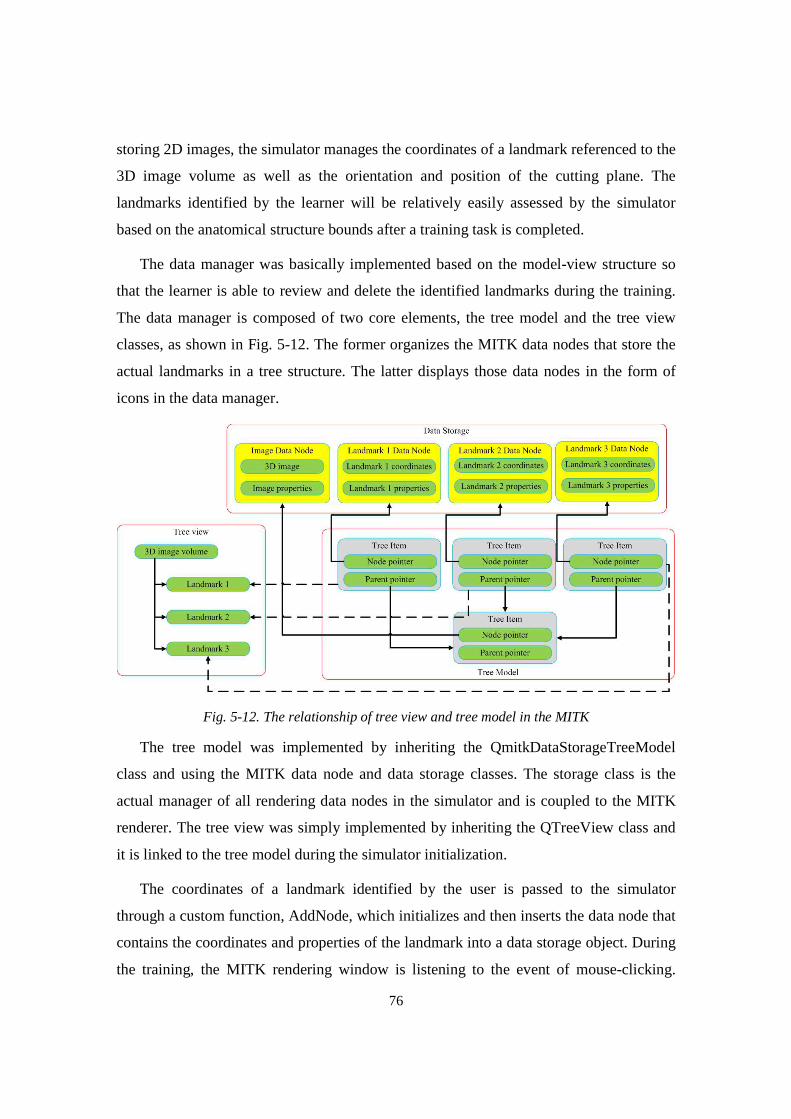
76

storing 2D images, the simulator manages the coordinates of a landmark referenced to the

3D image volume as well as the orientation and position of the cutting plane. The

landmarks identified by the learner will be relatively easily assessed by the simulator

based on the anatomical structure bounds after a training task is completed.

The data manager was basically implemented based on the model-view structure so

that the learner is able to review and delete the identified landmarks during the training.

The data manager is composed of two core elements, the tree model and the tree view

classes, as shown in Fig. 5-12. The former organizes the MITK data nodes that store the

actual landmarks in a tree structure. The latter displays those data nodes in the form of

icons in the data manager.

Fig. 5-12. The relationship of tree view and tree model in the MITK

The tree model was implemented by inheriting the QmitkDataStorageTreeModel

class and using the MITK data node and data storage classes. The storage class is the

actual manager of all rendering data nodes in the simulator and is coupled to the MITK

renderer. The tree view was simply implemented by inheriting the QTreeView class and

it is linked to the tree model during the simulator initialization.

The coordinates of a landmark identified by the user is passed to the simulator

through a custom function, AddNode, which initializes and then inserts the data node that

contains the coordinates and properties of the landmark into a data storage object. During

the training, the MITK rendering window is listening to the event of mouse-clicking.

77

Once the event is detected, the coordinates of the clicked point referenced to a given 3D

image, as described in the previous section, are provided to the custom function.

5.8 Implementation of a Dynamic Fetal Heart

During an ultrasound examination, a sonographer usually inspects if a fetus is alive or

not at the beginning of the examination, based on observing a beating fetal heart.

Accordingly, a generic 4D fetal heart was integrated into the simulator to improve the

overall realism. The beating heart is not intended to provide any diagnostic information.

The 2D image data used for generating the 4D fetal heart image volumes were

acquired at University of Massachusetts Memorial Medical Center using a Philips iU22

ultrasound system and the Stradwin software. A sonographer slowly moved the

transducer over the fetal heart to acquire a number of 2D images. Based on the actual

heart rate measured by the ultrasound machine and the timestamps of the collected 2D

images, eleven 3D fetal heart image volumes having same dimensions were created [57].

Each image volume represents a specific moment in the cardiac cycle of the fetal heart.

To implement a beating fetal heart, the simulator iteratively renders these 3D image

volumes in a predetermined sequence and rate while the user is scanning the PSS. Instead

of inserting the 4D fetal heart volumes into the 3D training image volume, which will

lead to eleven identical 3D training image volumes except that each has different

stationary fetal heart, the simulator dynamically blends the fetal heart into the 2D image

when a cutting plane intersects the fetal heart image volume. The eleven fetal heart image

volumes are a part of every training set and are loaded with the associated 3D training

image volume into the data manager but they are stored in a different data storage object.

During the generation of a 2D image, the simulator calls a custom function in the MITK,

NextHeartVolume, to sequentially retrieve a specific fetal heart image volume for the 2D

image reslicer so that the user can visually observe a beating fetal heart with a rate of 120

beats per minute.

To simplify the rendering process, the geometry of the fetal heart was considered a

sphere (S) so that it could be modeled by two parameters, the sphere center and radius.

They were determined offline based on the position and size of the fetal heart of a

78

selected 3D image volume. An experienced sonographer helped us with placing the fetal

heart at the proper location inside a given image volume using the SliceBrowser and the

simulator. These two parameter (position and size) were then stored in the parameter file

associated to the 3D image volume.

The generation of a 2D image basically follows the process described in Chapter 5.5,

as shown in Fig. 5-13. For a specific pixel P of the cutting plane, the simulator first

transforms P’s coordinates into its corresponding coordinates in the 3D image volume

space and then examines if the transformed coordinates are within the region defined by

the sphere model S. The result determines if the simulator calculates the pixel intensity,

based on either the 3D image volume (negative answer) or a specific fetal heart image

volume (positive answer). This approach did present a problem that the 2D image was

discontinuous at the boundary between the fetal heart sphere and the 3D image volume.

To resolve this problem, we introduced an extra sphere (S’) having the same center as the

sphere model S but with a larger radius. If the transformed coordinates of the pixel P is

within the model S’ and outside the model S, the pixel intensity is calculated based on the

3D image volume and the fetal heart volume by using alpha blending, as shown in eq. (5-

14), where �1and �2 are the intensities of the transformed pixels in the fetal heart image

volume and the 3D image volume, respectively; Ç is the distance from the transformed

pixel to the center of the model S.

� = ��Ç +��(1 − Ç) (5-14)

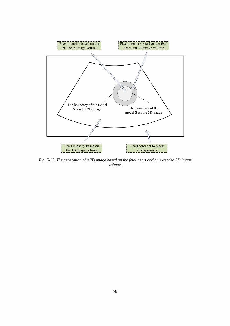
79

Fig. 5-13. The generation of a 2D image based on the fetal heart and an extended 3D image volume.

80

Chapter 6

The Structured Obstetric Ultrasound Training Curriculu m

and Automated Training Assessment

The use of simulators in obstetrics ultrasound training overcomes the limitation

inherent in conventional training: that the training is dependent on the availability of

pregnant subjects to scan and of ultrasound machines to use. However, without an

integrated assessment, simulator-based ultrasound training still greatly relies on an

instructor’s guidance and evaluation. In basic or intermediate obstetric ultrasound

training, a learner only aims to acquire basic scan skills and diagnostic ability. The

training guidance and assessment at these levels of training can potentially be transferred

to the simulator if we can assume that the scan procedure and evaluation follows standard

obstetric ultrasound examination guidelines. The learner can then complete the training

without an instructor or with limited guidance at the beginning via the simulator-

supervised or self-paced training.

A key to implement the self-paced training is to make the simulator provide the

learner with a structured training curriculum and an appropriate automatic assessment. In

this chapter, we first present implementation of the obstetric ultrasound training

curriculum that is composed of a set of tasks. Then, we present the segmentation and

modelling algorithms, which are used to create the landmark bounds. Finally, we describe

the automatic assessment of each task.

81

6.1 Introduction of the Obstetric Ultrasound Examination

To design appropriate self-paced training, we must understand the procedure of an

obstetric ultrasound examination, the best time(s) to perform the scan and the criteria to

evaluate scan performance. A 40-week pregnancy is commonly divided into three stages,

the first trimester (0-13 weeks), the second trimester (14 to 26 weeks) and the third

trimester (27 to 40 weeks), each of which is marked by specific fetal developments.

Accordingly, the AIUM classifies fetal sonographic examinations into four types [82]: 1)

the first trimester ultrasound examination, (2) the standard second or third trimester

examination, (3) the limited examination, and (4) the specialized examination. The

examination in first trimester is focused on confirming the intrauterine pregnancy and

date of the pregnancy, and monitoring the pregnancy development. Gestational sac(s), an

important sign of early pregnancy, is observed and measured in the first trimester. The

examinations in second and third trimesters cover the evaluation of fetal presentation,

fetal and placenta position and biometric measurements. The last two examinations are

performed when a special medical question or an anatomy needs to be investigated.

Currently, the simulator is only focused on providing ultrasound training for the

standard second or third trimester examination (standard ultrasound examination), for

two reasons: 1) in the late stage of the second trimester of pregnancy and the early stage

of the third trimester (24 – 36 weeks), many important anatomical structures can be

measured due to the fetus having developed sufficiently in size; 2) the examination is a

part of routine pregnancy care so that all pregnant women are required to receive this

examination.

In a regular standard ultrasound examination, a sonographer first evaluates fetal

cardiac activities, fetal presentation and maternal anatomy (cervix, bladder, etc.). Then he

or she examines placenta and fetal positions in a sagittal or transverse view. The

definitions of two views are shown in Fig. 6-1. The sagittal view is a cutting plane that

passes anterior and posterior of a body and the transverse view is a cutting plane that

divides the body into superior and interior parts. Following the examination of the

placental and fetal positions, the sonographer qualitatively estimates amniotic fluid

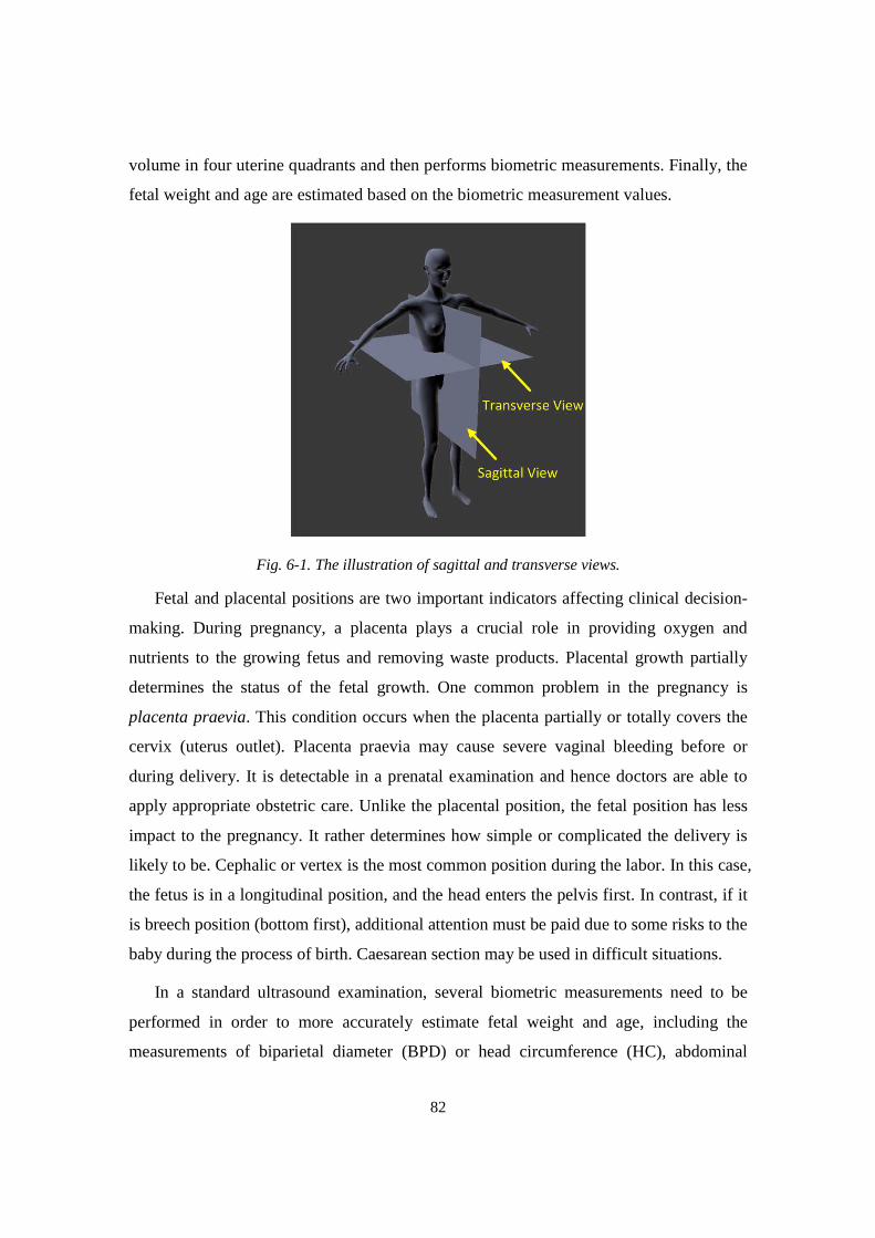
82

volume in four uterine quadrants and then performs biometric measurements. Finally, the

fetal weight and age are estimated based on the biometric measurement values.

Fig. 6-1. The illustration of sagittal and transverse views.

Fetal and placental positions are two important indicators affecting clinical decision-

making. During pregnancy, a placenta plays a crucial role in providing oxygen and

nutrients to the growing fetus and removing waste products. Placental growth partially

determines the status of the fetal growth. One common problem in the pregnancy is

placenta praevia. This condition occurs when the placenta partially or totally covers the

cervix (uterus outlet). Placenta praevia may cause severe vaginal bleeding before or

during delivery. It is detectable in a prenatal examination and hence doctors are able to

apply appropriate obstetric care. Unlike the placental position, the fetal position has less

impact to the pregnancy. It rather determines how simple or complicated the delivery is

likely to be. Cephalic or vertex is the most common position during the labor. In this case,

the fetus is in a longitudinal position, and the head enters the pelvis first. In contrast, if it

is breech position (bottom first), additional attention must be paid due to some risks to the

baby during the process of birth. Caesarean section may be used in difficult situations.

In a standard ultrasound examination, several biometric measurements need to be

performed in order to more accurately estimate fetal weight and age, including the

measurements of biparietal diameter (BPD) or head circumference (HC), abdominal

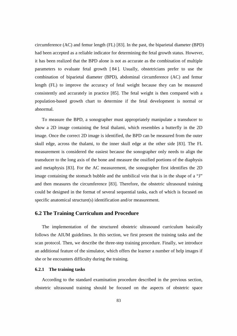
83

circumference (AC) and femur length (FL) [83]. In the past, the biparietal diameter (BPD)

had been accepted as a reliable indicator for determining the fetal growth status. However,

it has been realized that the BPD alone is not as accurate as the combination of multiple

parameters to evaluate fetal growth [ 84 ]. Usually, obstetricians prefer to use the

combination of biparietal diameter (BPD), abdominal circumference (AC) and femur

length (FL) to improve the accuracy of fetal weight because they can be measured

consistently and accurately in practice [85]. The fetal weight is then compared with a

population-based growth chart to determine if the fetal development is normal or

abnormal.

To measure the BPD, a sonographer must appropriately manipulate a transducer to

show a 2D image containing the fetal thalami, which resembles a butterfly in the 2D

image. Once the correct 2D image is identified, the BPD can be measured from the outer

skull edge, across the thalami, to the inner skull edge at the other side [83]. The FL

measurement is considered the easiest because the sonographer only needs to align the

transducer to the long axis of the bone and measure the ossified portions of the diaphysis

and metaphysis [83]. For the AC measurement, the sonographer first identifies the 2D

image containing the stomach bubble and the umbilical vein that is in the shape of a “J”

and then measures the circumference [83]. Therefore, the obstetric ultrasound training

could be designed in the format of several sequential tasks, each of which is focused on

specific anatomical structure(s) identification and/or measurement.

6.2 The Training Curriculum and Procedure

The implementation of the structured obstetric ultrasound curriculum basically

follows the AIUM guidelines. In this section, we first present the training tasks and the

scan protocol. Then, we describe the three-step training procedure. Finally, we introduce

an additional feature of the simulator, which offers the learner a number of help images if

she or he encounters difficulty during the training.

6.2.1 The training tasks

According to the standard examination procedure described in the previous section,

obstetric ultrasound training should be focused on the aspects of obstetric space

84

orientation and critical biometric measurement. In addition to the hands-on practice, a

complete training curriculum should include a session teaching basic clinical and medical

ultrasound knowledge. Thus, we defined a module-based obstetric ultrasound training

curriculum, covering the above material in three modules, as described below.

Module 1: Basic concept and physics of medical ultrasound

• 1a: Concept: Describe sound waves, concept of frequency and then frequency and

wavelength in medical ultrasound.

• 1b: Ultrasound advantages: Ultrasound is safe (no radiation), low-cost, high

availability in contrast to other image modality.

• 1c: Image formation: Explain the principle of sound to image conversion. Transmits

the sound wave and then format 2D image based on reflected echoes.

• 1d: Tissue interaction: Explain attenuation, reflection, transmission, scattering of

sound in tissues.

• 1e: Medical Ultrasound: Introduce diagnostic and non-diagnostic ultrasound.

• 1f: Transducer: Illuminate piezoelectric 1D array with different scan surface. Three

basics are linear, convex, phase array transducer.

• 1g: Image Modes: Illuminate A-Mode, B-Mode, C-Mode, M-Mode and Doppler

Mode ultrasound.

• 1h: Knobology: Explain some basic knowledge of the controls that you will encounter

on the console of an ultrasound scanner is important. Such as scan depth, overall

gaining, image mode.

• 1i: Skills in ultrasound scan: Develop good understanding in anatomy and physiology

of the organs as well as abnormalities and pathologies and their appearance in

ultrasound images.

Module 2: Orientation to the obstetric space

• 2a: Determine maternal anatomies: Locate an image plane that contains both the

bladder and the internal os of cervix; find bladder/lower uterine segment/cervix.

85

• 2b: Determine fetal position: Show longitudinal lower segment image with presenting

part and click on the presenting part. Answer the question that what is the fetal

position (cephalic, breech or transverse).

• 2c: Determine placenta position: Demonstrate a longitudinal lower segment image

and transverse mid-uterine and click on the placenta. Answer the question that what is

the placenta position (anterior, posterior, fundal or previa).

• 2d: Determine amniotic fluid index: Find amniotic fluid and measure maximal

vertical pocket depth in 4 quadrants, which are right upper quadrant (RUQ), left

upper quadrant (LUQ), lower left quadrant (LLQ) and right lower quadrant (RLQ).

Module 3: Fetal landmarks and biometry

• 3a: Measure biparietal diameter: Show transverse view of head with thalami, no

posterior fossa structures, along with occipitofrontal diameter to calculate head

circumference. Freeze 2D image and appropriately place the caliper to measure BPD.

• 3b: Measure abdominal circumference: Transverse, level of stomach bubble and “J”

shape of umbilical vein, no ribs, measure anterior-posterior and lateral diameters.

Freeze 2D image and appropriately place the caliper to measure two diameters.

• 3c: Measure femur length: Measure femur closest to and parallel to the transducer.

Freeze 2D image and appropriately place the caliper to measure FL.

• 3d: Estimate fetal weight: Simulator will calculate estimated fetal weight using

standard growth curves based on the BPD, AC and FL.

The training tasks in Modules 2 and 3 follow the AIUM’s practice guidelines except

for measurement of fetal heart rate and for carrying out a fetal anatomy survey. The fetal

heart, as stated in Chapter 5.8, was implemented with a fixed rate, 120 beats per minute.

Therefore, the heart rate is not included in the simulator training. The anatomy survey is

commonly necessary when technical limitations in the standard examination degrade

anatomical evaluation due to imaging artifacts from acoustic shadowing or a sonographer

finds suspected abnormality exists in a fetus.

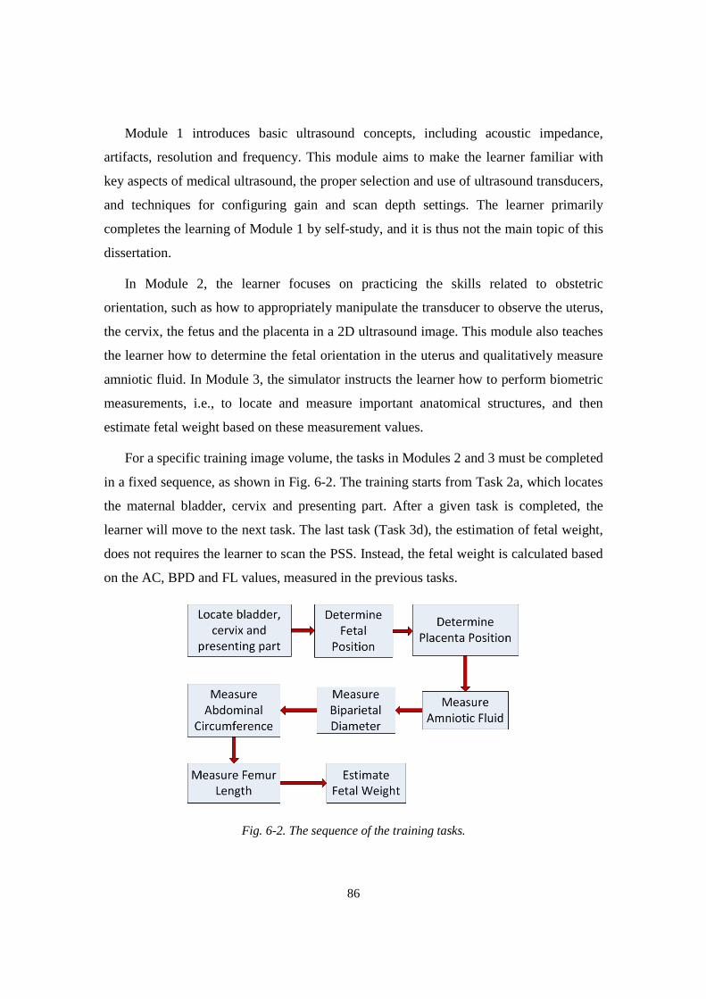
86

Module 1 introduces basic ultrasound concepts, including acoustic impedance,

artifacts, resolution and frequency. This module aims to make the learner familiar with

key aspects of medical ultrasound, the proper selection and use of ultrasound transducers,

and techniques for configuring gain and scan depth settings. The learner primarily

completes the learning of Module 1 by self-study, and it is thus not the main topic of this

dissertation.

In Module 2, the learner focuses on practicing the skills related to obstetric

orientation, such as how to appropriately manipulate the transducer to observe the uterus,

the cervix, the fetus and the placenta in a 2D ultrasound image. This module also teaches

the learner how to determine the fetal orientation in the uterus and qualitatively measure

amniotic fluid. In Module 3, the simulator instructs the learner how to perform biometric

measurements, i.e., to locate and measure important anatomical structures, and then

estimate fetal weight based on these measurement values.

For a specific training image volume, the tasks in Modules 2 and 3 must be completed

in a fixed sequence, as shown in Fig. 6-2. The training starts from Task 2a, which locates

the maternal bladder, cervix and presenting part. After a given task is completed, the

learner will move to the next task. The last task (Task 3d), the estimation of fetal weight,

does not requires the learner to scan the PSS. Instead, the fetal weight is calculated based

on the AC, BPD and FL values, measured in the previous tasks.

Fig. 6-2. The sequence of the training tasks.

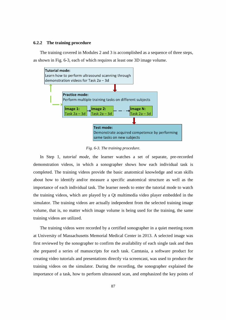
87

6.2.2 The training procedure

The training covered in Modules 2 and 3 is accomplished as a sequence of three steps,

as shown in Fig. 6-3, each of which requires at least one 3D image volume.

Fig. 6-3. The training procedure.

In Step 1, tutorial mode, the learner watches a set of separate, pre-recorded

demonstration videos, in which a sonographer shows how each individual task is

completed. The training videos provide the basic anatomical knowledge and scan skills

about how to identify and/or measure a specific anatomical structure as well as the

importance of each individual task. The learner needs to enter the tutorial mode to watch

the training videos, which are played by a Qt multimedia video player embedded in the

simulator. The training videos are actually independent from the selected training image

volume, that is, no matter which image volume is being used for the training, the same

training videos are utilized.

The training videos were recorded by a certified sonographer in a quiet meeting room

at University of Massachusetts Memorial Medical Center in 2013. A selected image was

first reviewed by the sonographer to confirm the availability of each single task and then

she prepared a series of manuscripts for each task. Camtasia, a software product for

creating video tutorials and presentations directly via screencast, was used to produce the

training videos on the simulator. During the recording, the sonographer explained the

importance of a task, how to perform ultrasound scan, and emphasized the key points of

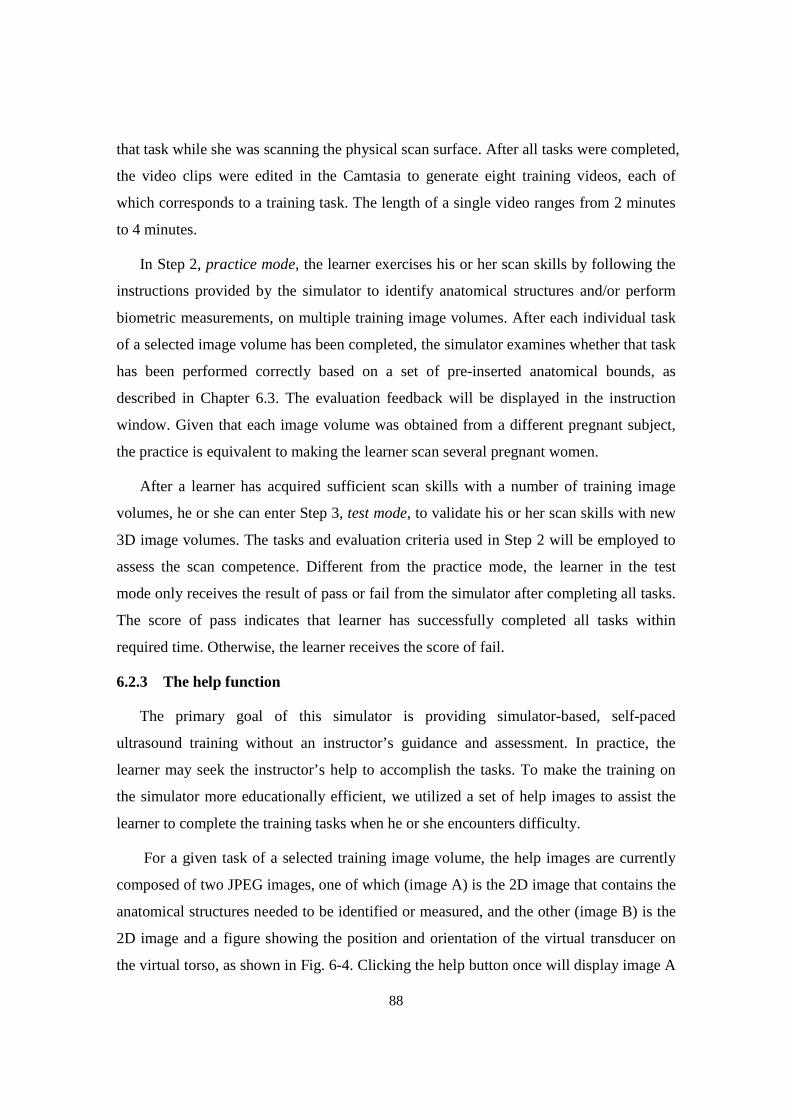
88

that task while she was scanning the physical scan surface. After all tasks were completed,

the video clips were edited in the Camtasia to generate eight training videos, each of

which corresponds to a training task. The length of a single video ranges from 2 minutes

to 4 minutes.

In Step 2, practice mode, the learner exercises his or her scan skills by following the

instructions provided by the simulator to identify anatomical structures and/or perform

biometric measurements, on multiple training image volumes. After each individual task

of a selected image volume has been completed, the simulator examines whether that task

has been performed correctly based on a set of pre-inserted anatomical bounds, as

described in Chapter 6.3. The evaluation feedback will be displayed in the instruction

window. Given that each image volume was obtained from a different pregnant subject,

the practice is equivalent to making the learner scan several pregnant women.

After a learner has acquired sufficient scan skills with a number of training image

volumes, he or she can enter Step 3, test mode, to validate his or her scan skills with new

3D image volumes. The tasks and evaluation criteria used in Step 2 will be employed to

assess the scan competence. Different from the practice mode, the learner in the test

mode only receives the result of pass or fail from the simulator after completing all tasks.

The score of pass indicates that learner has successfully completed all tasks within

required time. Otherwise, the learner receives the score of fail.

6.2.3 The help function

The primary goal of this simulator is providing simulator-based, self-paced

ultrasound training without an instructor’s guidance and assessment. In practice, the

learner may seek the instructor’s help to accomplish the tasks. To make the training on

the simulator more educationally efficient, we utilized a set of help images to assist the

learner to complete the training tasks when he or she encounters difficulty.

For a given task of a selected training image volume, the help images are currently

composed of two JPEG images, one of which (image A) is the 2D image that contains the

anatomical structures needed to be identified or measured, and the other (image B) is the

2D image and a figure showing the position and orientation of the virtual transducer on

the virtual torso, as shown in Fig. 6-4. Clicking the help button once will display image A

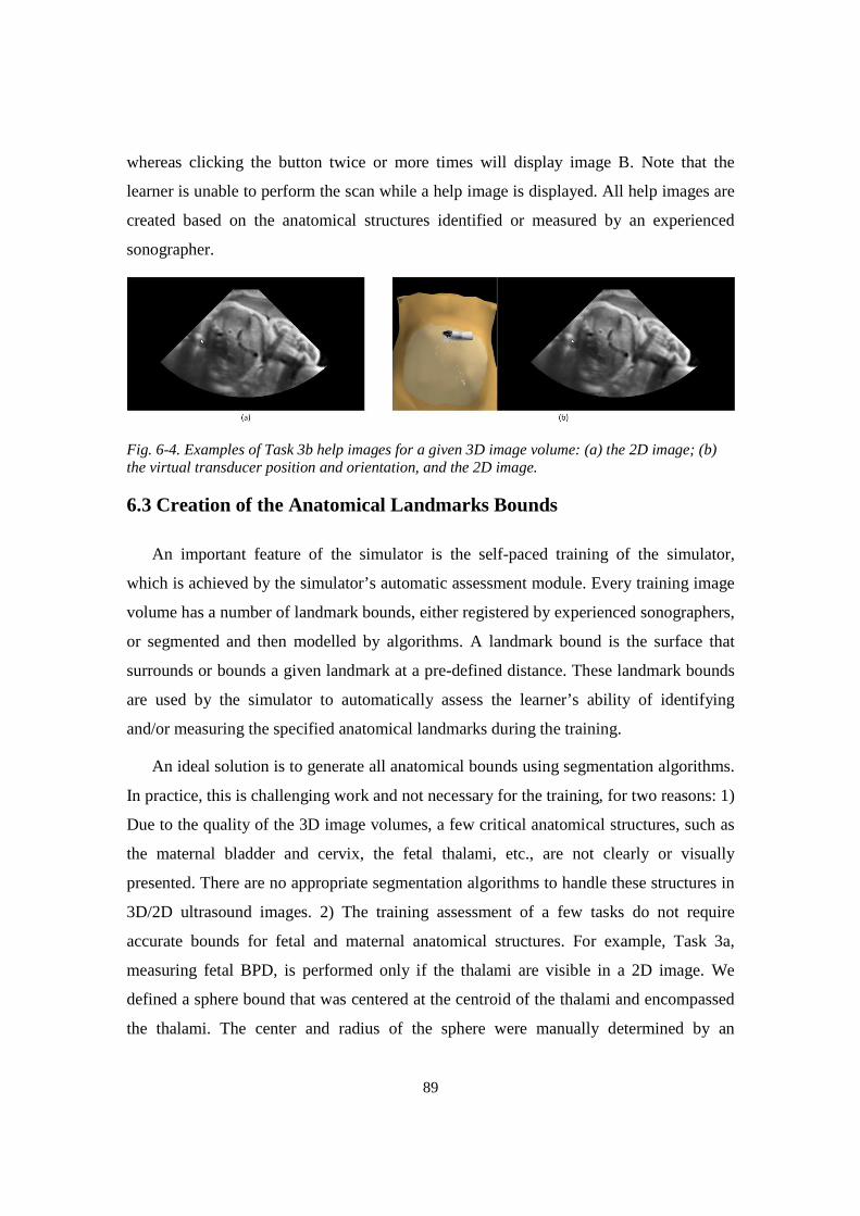
89

whereas clicking the button twice or more times will display image B. Note that the

learner is unable to perform the scan while a help image is displayed. All help images are

created based on the anatomical structures identified or measured by an experienced

sonographer.

Fig. 6-4. Examples of Task 3b help images for a given 3D image volume: (a) the 2D image; (b) the virtual transducer position and orientation, and the 2D image.

6.3 Creation of the Anatomical Landmarks Bounds

An important feature of the simulator is the self-paced training of the simulator,

which is achieved by the simulator’s automatic assessment module. Every training image

volume has a number of landmark bounds, either registered by experienced sonographers,

or segmented and then modelled by algorithms. A landmark bound is the surface that

surrounds or bounds a given landmark at a pre-defined distance. These landmark bounds

are used by the simulator to automatically assess the learner’s ability of identifying

and/or measuring the specified anatomical landmarks during the training.

An ideal solution is to generate all anatomical bounds using segmentation algorithms.

In practice, this is challenging work and not necessary for the training, for two reasons: 1)

Due to the quality of the 3D image volumes, a few critical anatomical structures, such as

the maternal bladder and cervix, the fetal thalami, etc., are not clearly or visually

presented. There are no appropriate segmentation algorithms to handle these structures in

3D/2D ultrasound images. 2) The training assessment of a few tasks do not require

accurate bounds for fetal and maternal anatomical structures. For example, Task 3a,

measuring fetal BPD, is performed only if the thalami are visible in a 2D image. We

defined a sphere bound that was centered at the centroid of the thalami and encompassed

the thalami. The center and radius of the sphere were manually determined by an

90

experienced sonographer using the simulator. A common situation is if the 2D image is

too far away from the bound center, the fetal skull on the 2D image may be too small for

measuring the correct diameter. Thus, the bound does not need to exactly model the

thalami geometry. Currently, for a given 3D image volume, all landmark bounds except

the placenta and the fetal head are modelled by a number of spheres with different radii

and determined on the simulator under the guidance of an experienced sonographer.

These bounds were created for the maternal bladder, the cervix, the thalami, the fetal

stomach bubble, the umbilical vein and the two ends of the femur. The BPD, FL and AC

are also manually measured by the experienced sonographer and then stored with above

landmark bounds in the same file.

In an actual ultrasound examination, the fetal position is determined through

observing the presenting part in a 2D image, such as the fetal head used in Task 2b.

However, in practice, more than one 2D image can be used to determine the fetal position.

This poses a challenge in designing the assessment for Task 2b if the assessment is only

based on the orientation and position of the sham transducer. An alternative is asking the

learner to click the fetal head on the 2D image to inform the simulator of his or her

identification, in addition to the sham transducer’s orientation and position. Similarly, the

creation of the placenta bound faces the same challenge, as stated above. Moreover, the

placenta in the uterus usually resembles a flat crescent [86] and thereby is difficult to be

modeled by a simple shape. Given that the geometries and characters of these two

anatomical structures are different, we needed to implement different segmentation and

modelling algorithms to create 3D fetal head and placenta bounds for a given 3D image

volume.

6.3.1 Overview of segmentation algorithms

In general, image segmentation approaches that have been used in medical images

can be categorized into several types, including the morphological operators based, the

boundary based, the region based, the probabilistic model based, or the combination of

two or more methods.

91

Morphological operator based approaches

The initial methods for automatic segmentation of fetal anatomies were mainly based

on morphological operators. This approach usually contains several steps to generate

binary images for segmentation, such as noise suppression, image contrast enhancement,

morphological operation, thresholding and skeletonization (find the thinnest

representation of the original pattern that preserves the topology). In a study of fetal head

segmentation [87], the authors relied on the acoustic property of bones, i.e., their high

density (or high acoustic impedance), to detect a fetal skull. A boundary between soft

tissue and a bone structure reflects more ultrasound energy back to the transducer so that

such structures appear much brighter than boundaries between relatively similar soft

tissues in ultrasound images. The 2D image containing a fetal skull was pre-processed by

low-pass filters, then classified as foreground and background areas by the K-mean

algorithm and finally processed by morphologic open and close operations. The iterative

Hough transform was applied the processed image to find an ellipse being the best fit for

the fetal skull. This method has shown a high level of consistency. In another study, the

researchers also utilized morphologic operators to segment a fetal femur [88], in which

similar steps were applied to ultrasound images. The morphologic operator based method

usually shows a high r-value (correlation coefficient) when comparing to the

segmentation results completed by experienced sonographers; however, this method

partially depends on the quality of preprocessing approaches to remove objects that are

not the segmentation target. The users have to experimentally optimize parameters for

preprocessing filters or classifiers.

Boundary based approaches

Boundary based approaches commonly utilize gradients information inside 2D

images to locate objects’ boundaries. The early methods include first derivative Sobel

operators or second derivative Laplacian operators. These simple operators are sensitive

to image noise so that they cannot appropriately segment objects in ultrasound images.

Active contour and level set are two most widely used boundary based approaches.

Active contour (Snakes), a very popular segmentation algorithm (>4000 citations),

92

locates the edges of objects through minimizing an energy function. The object contour ¾: q0,1r → Ω is evolved as shown eq. 6-1:

Ë(¾(1)) = −Ì |∇º(¾(1))|��1 + \� Ì |¾x(1)|��1 + \� Ì |¾xx(1)|��1 (6-1)

where ¾x and ¾xx denote the first and second derivatives with respect to the parameter 1;

Ω denotes the 2D image. The first term is external energy or image force and usually

favors the location of large gradient. The second and third terms controls the length and

stiffness of the contour. In one study [89], the authors used this approach to detect a fetal

head. The user was required to mark a single point near the center of the head and then

their algorithm automatically calculated the initial contour. This study showed that the

identified contours had very high r-value (>0.99) in comparison to manual segmentation

if the initial boundary can be successfully located near the object’s edge. However, their

experiment also showed many segmentation failures. The active counter often has several

problems when applied to ultrasound images: 1) the users must place control points near

the boundary of objects; 2) the contour is often trapped in local minima if inappropriate

initialization is used at which point the contour needs manual correction; 3) it is less

accurate in tackling objects with open boundary; 4) it is sensitive to noise.

Probabilistic model based approaches

Probabilistic model based approaches have a long history in medical image

segmentation. Initially, these approaches were based only on statistical analysis and

applied on discrete pixels without considering any structural information of the region

[90], such as using thresholding method [91]. The lack of integrating objects’ geometries

usually results in the identified pixels not being contiguous. It easily misses isolated

pixels within the region (especially near the boundaries of the region). Segmentation

outcomes become worse if images are noisy, simply because it is more likely that a

pixel’s intensity does not represent the normal intensity in a region. Many recent

probabilistic segmentation studies heavily relied on the Bayes rule to locate an object’s

boundary [92, 93] in combination of other approaches. In [94], Sandra et al. utilized

maximum likelihood parametric deformable models, in combination of the active contour,

to identify fetal skulls and femurs under the assumption that the intensity distribution of

93

ultrasound images follows the Rayleigh distribution. Eq. (6-2) defines a joint probability

density function of a given image with a contour of \(Î). �(Ï|�, �) = ∏ �(ÏI|�I)I∈Ò(�(Î)) ∏ �(ÏI|�Ó)I∈Ô(�(Î)) (6-2)

where Ï� denotes ith pixel of the image; º(\(Î)) and ¿(\(Î)) denote the inside or

outside region of the contour, respectively. Î is the parameter set of the contour; �I and �Ó are the distribution factors of the regions inside and outside the contour, respectively.

By updating the �, � iteratively, the algorithm can find an appropriate parameter set Î′ that gives the maximum probability with the contour. Their experiment showed that the

algorithm presented a good outcome on synthesized ultrasound images but also that it

was not accurate on real ultrasound images.

Region based approaches

Region-based approaches are basically hybrid methods, usually based on a

probabilistic or statistics approach. Region growing, commonly statistics-based,

continuously examines neighboring pixels of a target region and determines whether they

should be added to the region on the basis of the homogeneity of spatially localized

features and properties until no more pixels meet the criteria [95]. In [95], the authors

used a seed to initialize the process under the assumption that the pixels inside a tissue

have similar intensities. If a new neighboring pixel is within the variance of the mean

intensity of the segmented region, it will be added into the region and then the region

mean intensity value and variance are reevaluated. Their experiment result has

demonstrated the feasibility of the region-growing based approach in medical image

segmentation, but the algorithm was still influenced by the seed point location and the

scan pattern [96]. An inappropriate region seed selection or pixel sorting order may result

in an incorrect segmentation [97]. Additionally, the region growing is sensitive to image

noise. Several automated region growing approaches have been developed, such as

checking the pixel intensity difference between a fixed amounts of distance [90], using a

co-occurrence matrix (texture extraction) to differentiate homogeneous regions from non-

homogeneous regions [98], or splitting an image histogram into several subintervals,

which represent different image regions [99], etc.

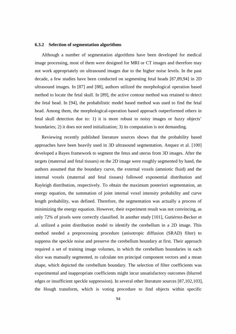
94

6.3.2 Selection of segmentation algorithms

Although a number of segmentation algorithms have been developed for medical

image processing, most of them were designed for MRI or CT images and therefore may

not work appropriately on ultrasound images due to the higher noise levels. In the past

decade, a few studies have been conducted on segmenting fetal heads [87,89,94] in 2D

ultrasound images. In [87] and [88], authors utilized the morphological operation based

method to locate the fetal skull. In [89], the active contour method was retained to detect

the fetal head. In [94], the probabilistic model based method was used to find the fetal

head. Among them, the morphological-operation based approach outperformed others in

fetal skull detection due to: 1) it is more robust to noisy images or fuzzy objects’

boundaries; 2) it does not need initialization; 3) its computation is not demanding.

Reviewing recently published literature sources shows that the probability based

approaches have been heavily used in 3D ultrasound segmentation. Anquez et al. [100]

developed a Bayes framework to segment the fetus and uterus from 3D images. After the

targets (maternal and fetal tissues) on the 2D image were roughly segmented by hand, the

authors assumed that the boundary curve, the external voxels (amniotic fluid) and the

internal voxels (maternal and fetal tissues) followed exponential distribution and

Rayleigh distribution, respectively. To obtain the maximum posteriori segmentation, an

energy equation, the summation of joint internal voxel intensity probability and curve

length probability, was defined. Therefore, the segmentation was actually a process of

minimizing the energy equation. However, their experiment result was not convincing, as

only 72% of pixels were correctly classified. In another study [101], Gutiérrez-Becker et

al. utilized a point distribution model to identify the cerebellum in a 2D image. This

method needed a preprocessing procedure (anisotropic diffusion (SRAD) filter) to

suppress the speckle noise and preserve the cerebellum boundary at first. Their approach

required a set of training image volumes, in which the cerebellum boundaries in each

slice was manually segmented, to calculate ten principal component vectors and a mean

shape, which depicted the cerebellum boundary. The selection of filter coefficients was

experimental and inappropriate coefficients might incur unsatisfactory outcomes (blurred

edges or insufficient speckle suppression). In several other literature sources [87,102,103],

the Hough transform, which is voting procedure to find objects within specific

95

geometries, was used to predict the coefficients of an elliptical fit for a given fetal head in

a 2D ultrasound image. The experimental results showed very positive segmentation

outcomes. Therefore, we chose the morphological-operation based Hough transform for

our fetal head segmentation.

After searching literature sources for segmenting the placenta either in a 2D or 3D

ultrasound image, we found that no study had been conducted. In an ultrasound image,

the placenta usually appears approximately homogeneous gray and is slightly different

from adjacent tissues. This appearance implies that a region-based approach may

outperform other algorithms in placenta segmentation. In addition, the region-based

approach is able to segment the complete placenta, which is essential for creating the 3D

placenta model used in the task assessment. Recently, a type of region based algorithms,

the cellular automata (CA) based approaches [104,105] has drawn lots of attention

because of its strengths in processing medical images by an evolving approach. The CA-

based approach is a discrete model that can be thought of as a number of cells on a

discrete grid. These cells can interact locally with their neighbors to propagate

information at a global scale. Each cell has finite number of states and its state is

dynamically updated when the cells interact. Of the CA-based segmentation algorithms,

the GrowCut is a simple, efficient approach, first proposed by Vezhnevets [104]. In the

GrowCut, every pixel of an image is treated as a cell with certain amount of energy. The

principle is that each single cell tries to conquer its neighbors until the energies of all

cells reach balance, or no cell energy is changed. Initially, the energy of each foreground

and background cells are manually set to +1 and -1, respectively, by the user, and all

others are set to zero. Thus, the GrowCut is semi-automatic segmentation algorithm. In a

recent study, Ghosh et al. [105] proposed an unsupervised GrowCut approach by

randomly labeling the cells with positive intensity values. Their algorithm was fully

automatic except that the threshold controlling the cell state transition needed to be

experimentally determined. In another study [106], the authors improved Vezhnevets’s

algorithms by adding a pre-initialization process before the actual GrowCut occurs. The

user could add new seeds in the pre-initialization to improve segmentation accuracy. The

experiments of the above GrowCut algorithms reached similar positive outcomes in

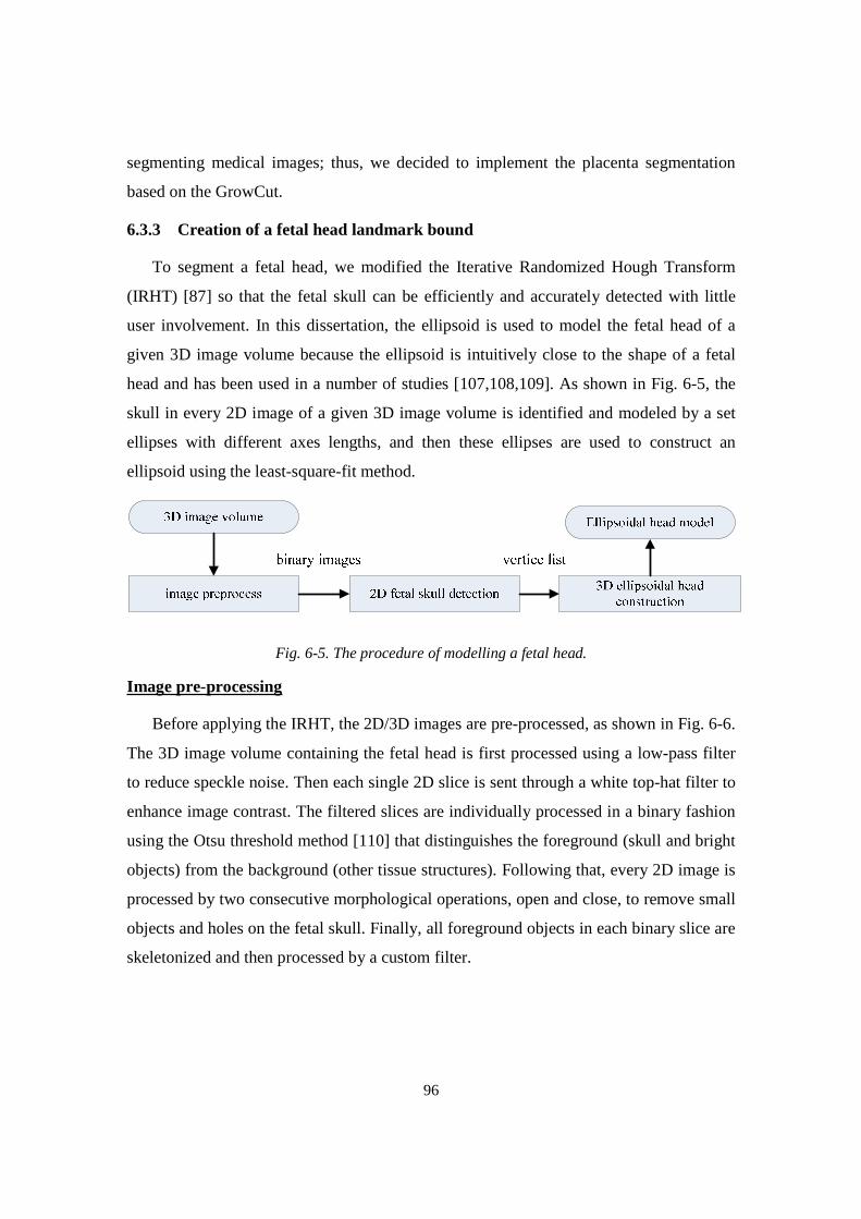
96

segmenting medical images; thus, we decided to implement the placenta segmentation

based on the GrowCut.

6.3.3 Creation of a fetal head landmark bound

To segment a fetal head, we modified the Iterative Randomized Hough Transform

(IRHT) [87] so that the fetal skull can be efficiently and accurately detected with little

user involvement. In this dissertation, the ellipsoid is used to model the fetal head of a

given 3D image volume because the ellipsoid is intuitively close to the shape of a fetal

head and has been used in a number of studies [107,108,109]. As shown in Fig. 6-5, the

skull in every 2D image of a given 3D image volume is identified and modeled by a set

ellipses with different axes lengths, and then these ellipses are used to construct an

ellipsoid using the least-square-fit method.

Fig. 6-5. The procedure of modelling a fetal head.

Image pre-processing

Before applying the IRHT, the 2D/3D images are pre-processed, as shown in Fig. 6-6.

The 3D image volume containing the fetal head is first processed using a low-pass filter

to reduce speckle noise. Then each single 2D slice is sent through a white top-hat filter to

enhance image contrast. The filtered slices are individually processed in a binary fashion

using the Otsu threshold method [110] that distinguishes the foreground (skull and bright

objects) from the background (other tissue structures). Following that, every 2D image is

processed by two consecutive morphological operations, open and close, to remove small

objects and holes on the fetal skull. Finally, all foreground objects in each binary slice are

skeletonized and then processed by a custom filter.

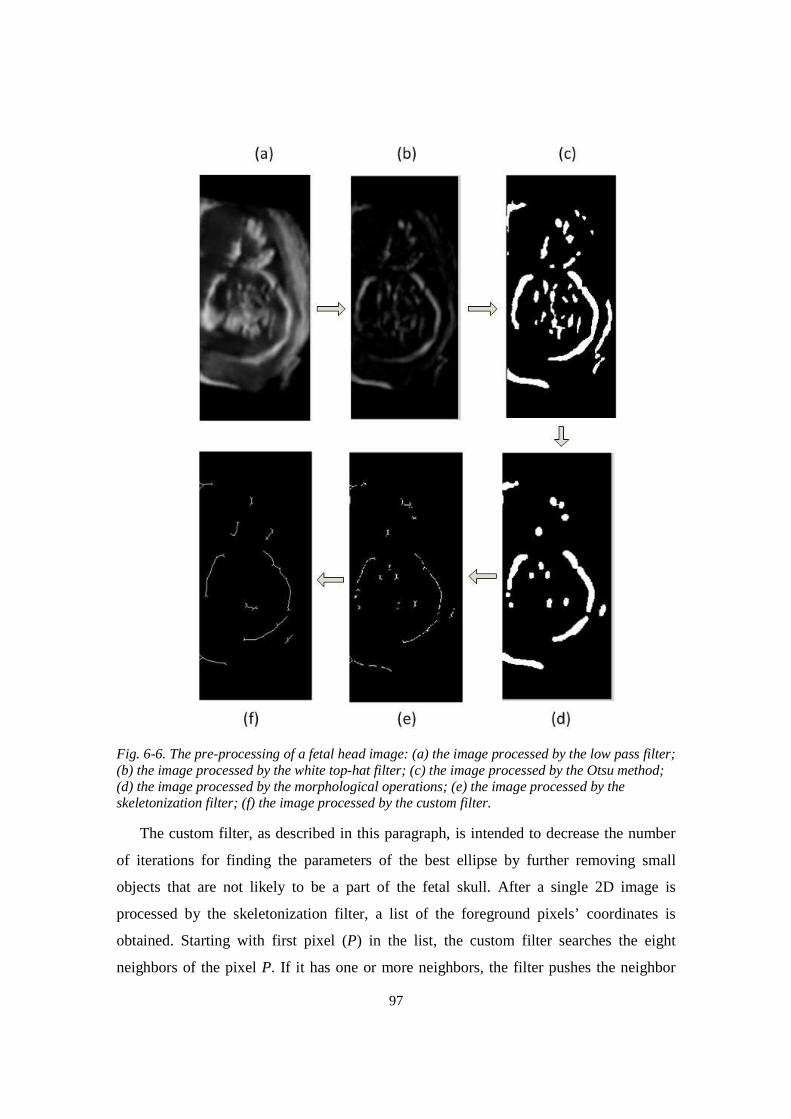
97

Fig. 6-6. The pre-processing of a fetal head image: (a) the image processed by the low pass filter; (b) the image processed by the white top-hat filter; (c) the image processed by the Otsu method; (d) the image processed by the morphological operations; (e) the image processed by the skeletonization filter; (f) the image processed by the custom filter.

The custom filter, as described in this paragraph, is intended to decrease the number

of iterations for finding the parameters of the best ellipse by further removing small

objects that are not likely to be a part of the fetal skull. After a single 2D image is

processed by the skeletonization filter, a list of the foreground pixels’ coordinates is

obtained. Starting with first pixel (P) in the list, the custom filter searches the eight

neighbors of the pixel P. If it has one or more neighbors, the filter pushes the neighbor

98

pixel(s) into a container and then repeats searching the neighbors of the pixels in the

container until the container is empty. Finally, the custom filter generates a set of separate

objects, each of which is a set of connected pixels, and then removes the small objects

based on an experimentally determined threshold.

Fetal head detection and modelling

An quadratic form of an ellipse is given in eq. (6-3) and can be described with a

parameter set s = (m, n, xc, yc, ψ) as shown in eq. (6-4), where 0 ≤ θ < 2π; (x, y)

represents a point on the ellipse; (xc, yc) is the center of the ellipse; m and n are the long

and short semi-axes and R is a rotation matrix derived from the rotation angle ψ as shown

in eq. (6-5).

U� + �+� + �U+ + �U + p+ + Õ = 0 (6-3)

ÖU+× = � ∗ Ö� cos �! sin � × + ÖUV+V× (6-4)

� = Ø�)1Ù −1�!Ù1�!Ù �)1Ù Ú (6-5)

To start the IRHT, the region of interest (ROI) is set to the whole 2D slice containing

the thalami. In addition, all elements of the parameter set s are set to zero. The IRHT has

been implemented in the following iterative steps. sk is the parameter set s in kth iteration,

k =1,2,….

1. If the input parameter set s exists, let sk = s (k=1), go to step 4. Otherwise continue

with step 2.

2. Randomly select five pixels from the list and solve eq. (6-4) to obtain a parameter

set s’. If it is valid, s’ is pushed into a five-column parameter array. Repeat until

the size of the parameter array is less than 1000.

3. Find ten most frequent elements in each column of the parameter array and

average them to generate a new parameter set sk

4. Adjust the ROI based on the center and radii of an ellipse defined by sk.

5. Eliminate the pixels that are out of ROI from the slice.

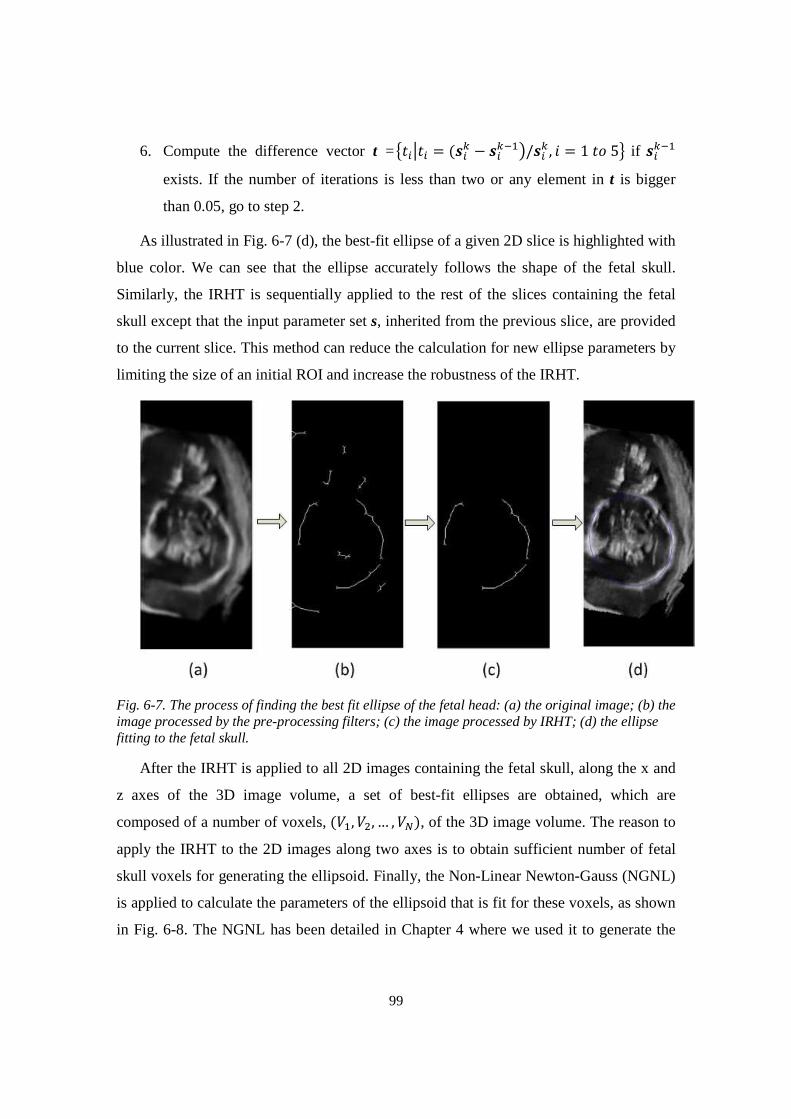
99

6. Compute the difference vector t =Û�IÜ�I = (�IM − �IMF�Ý/�IM , � = 1�)5ß if �IMF�

exists. If the number of iterations is less than two or any element in t is bigger

than 0.05, go to step 2.

As illustrated in Fig. 6-7 (d), the best-fit ellipse of a given 2D slice is highlighted with

blue color. We can see that the ellipse accurately follows the shape of the fetal skull.

Similarly, the IRHT is sequentially applied to the rest of the slices containing the fetal

skull except that the input parameter set s, inherited from the previous slice, are provided

to the current slice. This method can reduce the calculation for new ellipse parameters by

limiting the size of an initial ROI and increase the robustness of the IRHT.

Fig. 6-7. The process of finding the best fit ellipse of the fetal head: (a) the original image; (b) the image processed by the pre-processing filters; (c) the image processed by IRHT; (d) the ellipse fitting to the fetal skull.

After the IRHT is applied to all 2D images containing the fetal skull, along the x and

z axes of the 3D image volume, a set of best-fit ellipses are obtained, which are

composed of a number of voxels, (¼�, ¼�, … , ¼f), of the 3D image volume. The reason to

apply the IRHT to the 2D images along two axes is to obtain sufficient number of fetal

skull voxels for generating the ellipsoid. Finally, the Non-Linear Newton-Gauss (NGNL)

is applied to calculate the parameters of the ellipsoid that is fit for these voxels, as shown

in Fig. 6-8. The NGNL has been detailed in Chapter 4 where we used it to generate the

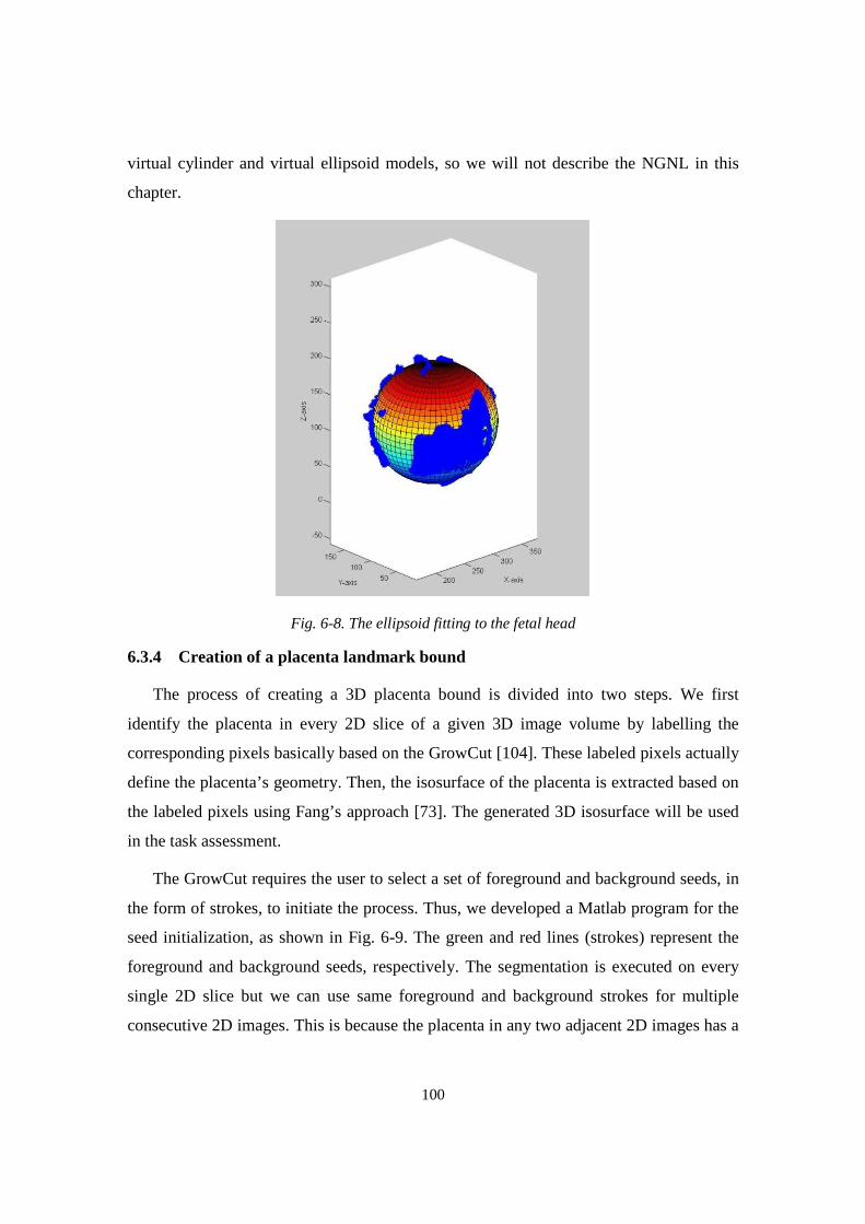
100

virtual cylinder and virtual ellipsoid models, so we will not describe the NGNL in this

chapter.

Fig. 6-8. The ellipsoid fitting to the fetal head

6.3.4 Creation of a placenta landmark bound

The process of creating a 3D placenta bound is divided into two steps. We first

identify the placenta in every 2D slice of a given 3D image volume by labelling the

corresponding pixels basically based on the GrowCut [104]. These labeled pixels actually

define the placenta’s geometry. Then, the isosurface of the placenta is extracted based on

the labeled pixels using Fang’s approach [73]. The generated 3D isosurface will be used

in the task assessment.

The GrowCut requires the user to select a set of foreground and background seeds, in

the form of strokes, to initiate the process. Thus, we developed a Matlab program for the

seed initialization, as shown in Fig. 6-9. The green and red lines (strokes) represent the

foreground and background seeds, respectively. The segmentation is executed on every

single 2D slice but we can use same foreground and background strokes for multiple

consecutive 2D images. This is because the placenta in any two adjacent 2D images has a

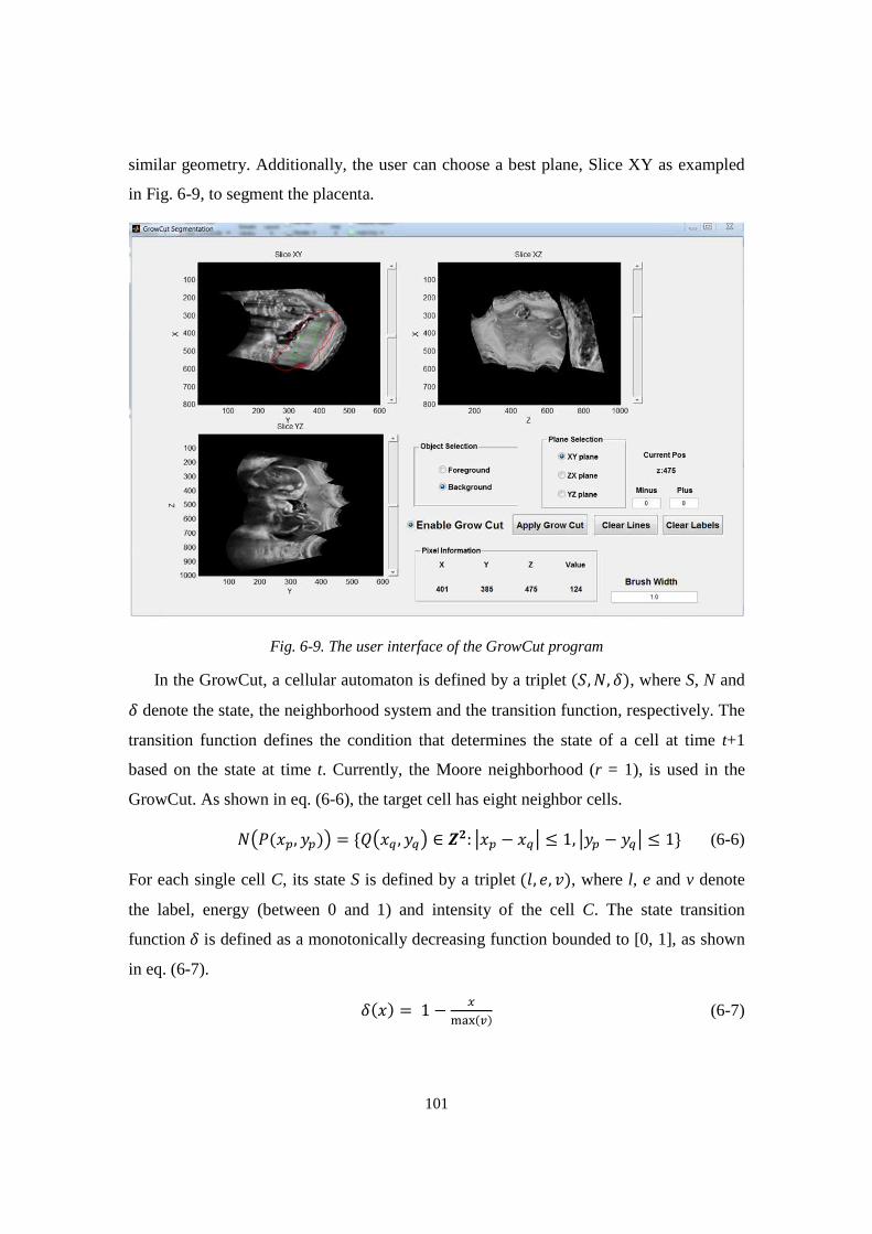
101

similar geometry. Additionally, the user can choose a best plane, Slice XY as exampled

in Fig. 6-9, to segment the placenta.

Fig. 6-9. The user interface of the GrowCut program

In the GrowCut, a cellular automaton is defined by a triplet (», b, à), where S, N and à denote the state, the neighborhood system and the transition function, respectively. The

transition function defines the condition that determines the state of a cell at time t+1

based on the state at time t. Currently, the Moore neighborhood (r = 1), is used in the

GrowCut. As shown in eq. (6-6), the target cell has eight neighbor cells.

báâ(U�, +�)Ý = {DáUG , +GÝ ∈ äå: ÜU� − UGÜ ≤ 1, Ü+� − +GÜ ≤ 1} (6-6)

For each single cell C, its state S is defined by a triplet (*, 3, \), where l, e and v denote

the label, energy (between 0 and 1) and intensity of the cell C. The state transition

function à is defined as a monotonically decreasing function bounded to [0, 1], as shown

in eq. (6-7).

à(U) = 1 − �³�´(�) (6-7)

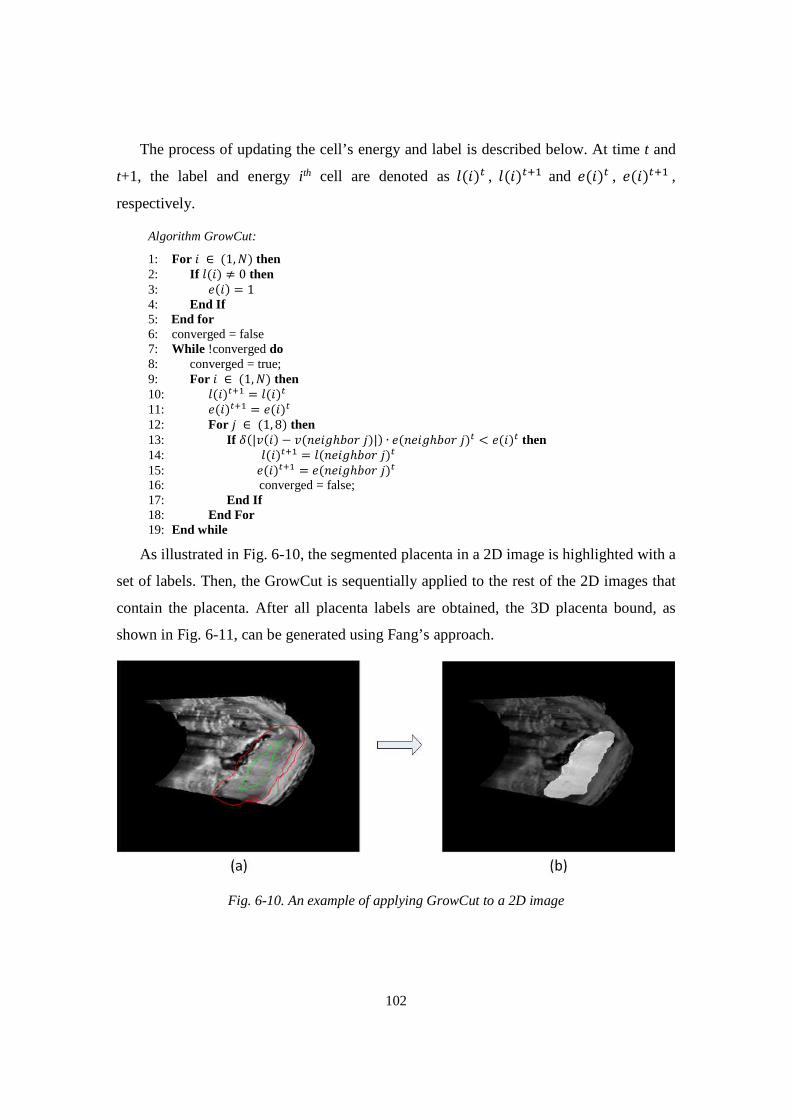
102

The process of updating the cell’s energy and label is described below. At time t and

t+1, the label and energy i th cell are denoted as *(�)` , *(�)`O� and 3(�)` , 3(�)`O� ,

respectively.

Algorithm GrowCut:

1: For � ∈ (1, b) then 2: If *(�) ≠ 0 then 3: 3(�) = 1 4: End If 5: End for 6: converged = false 7: While !converged do 8: converged = true; 9: For � ∈ (1, b) then 10: *(�)`O� = *(�)` 11: 3(�)`O� = 3(�)` 12: For � ∈ (1, 8) then 13: If à(|\(�) − \(!3�Õℎ�)(�)|) ∙ 3(!3�Õℎ�)(�)` < 3(�)` then 14: *(�)`O� = *(!3�Õℎ�)(�)` 15: 3(�)`O� = 3(!3�Õℎ�)(�)` 16: converged = false; 17: End If 18: End For 19: End while

As illustrated in Fig. 6-10, the segmented placenta in a 2D image is highlighted with a

set of labels. Then, the GrowCut is sequentially applied to the rest of the 2D images that

contain the placenta. After all placenta labels are obtained, the 3D placenta bound, as

shown in Fig. 6-11, can be generated using Fang’s approach.

Fig. 6-10. An example of applying GrowCut to a 2D image

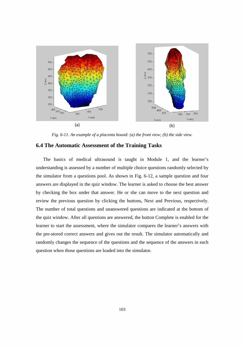
103

Fig. 6-11. An example of a placenta bound: (a) the front view; (b) the side view.

6.4 The Automatic Assessment of the Training Tasks

The basics of medical ultrasound is taught in Module 1, and the learner’s

understanding is assessed by a number of multiple choice questions randomly selected by

the simulator from a questions pool. As shown in Fig. 6-12, a sample question and four

answers are displayed in the quiz window. The learner is asked to choose the best answer

by checking the box under that answer. He or she can move to the next question and

review the previous question by clicking the buttons, Next and Previous, respectively.

The number of total questions and unanswered questions are indicated at the bottom of

the quiz window. After all questions are answered, the button Complete is enabled for the

learner to start the assessment, where the simulator compares the learner’s answers with

the pre-stored correct answers and gives out the result. The simulator automatically and

randomly changes the sequence of the questions and the sequence of the answers in each

question when those questions are loaded into the simulator.

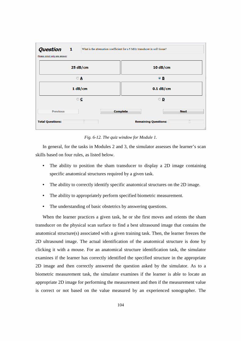
104

Fig. 6-12. The quiz window for Module 1.

In general, for the tasks in Modules 2 and 3, the simulator assesses the learner’s scan

skills based on four rules, as listed below.

• The ability to position the sham transducer to display a 2D image containing

specific anatomical structures required by a given task.

• The ability to correctly identify specific anatomical structures on the 2D image.

• The ability to appropriately perform specified biometric measurement.

• The understanding of basic obstetrics by answering questions.

When the learner practices a given task, he or she first moves and orients the sham

transducer on the physical scan surface to find a best ultrasound image that contains the

anatomical structure(s) associated with a given training task. Then, the learner freezes the

2D ultrasound image. The actual identification of the anatomical structure is done by

clicking it with a mouse. For an anatomical structure identification task, the simulator

examines if the learner has correctly identified the specified structure in the appropriate

2D image and then correctly answered the question asked by the simulator. As to a

biometric measurement task, the simulator examines if the learner is able to locate an

appropriate 2D image for performing the measurement and then if the measurement value

is correct or not based on the value measured by an experienced sonographer. The

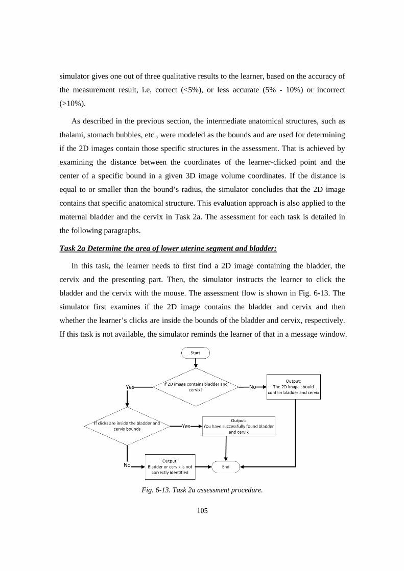
105

simulator gives one out of three qualitative results to the learner, based on the accuracy of

the measurement result, i.e, correct (<5%), or less accurate (5% - 10%) or incorrect

(>10%).

As described in the previous section, the intermediate anatomical structures, such as

thalami, stomach bubbles, etc., were modeled as the bounds and are used for determining

if the 2D images contain those specific structures in the assessment. That is achieved by

examining the distance between the coordinates of the learner-clicked point and the

center of a specific bound in a given 3D image volume coordinates. If the distance is

equal to or smaller than the bound’s radius, the simulator concludes that the 2D image

contains that specific anatomical structure. This evaluation approach is also applied to the

maternal bladder and the cervix in Task 2a. The assessment for each task is detailed in

the following paragraphs.

Task 2a Determine the area of lower uterine segment and bladder:

In this task, the learner needs to first find a 2D image containing the bladder, the

cervix and the presenting part. Then, the simulator instructs the learner to click the

bladder and the cervix with the mouse. The assessment flow is shown in Fig. 6-13. The

simulator first examines if the 2D image contains the bladder and cervix and then

whether the learner’s clicks are inside the bounds of the bladder and cervix, respectively.

If this task is not available, the simulator reminds the learner of that in a message window.

Fig. 6-13. Task 2a assessment procedure.

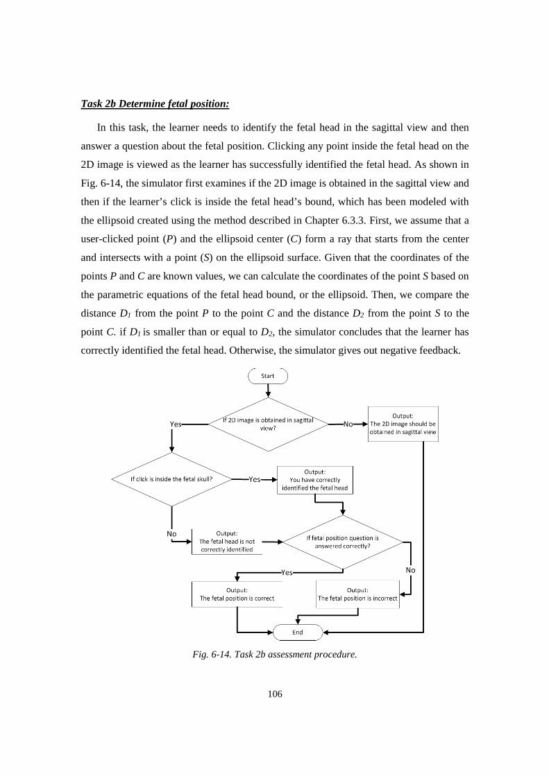
106

Task 2b Determine fetal position:

In this task, the learner needs to identify the fetal head in the sagittal view and then

answer a question about the fetal position. Clicking any point inside the fetal head on the

2D image is viewed as the learner has successfully identified the fetal head. As shown in

Fig. 6-14, the simulator first examines if the 2D image is obtained in the sagittal view and

then if the learner’s click is inside the fetal head’s bound, which has been modeled with

the ellipsoid created using the method described in Chapter 6.3.3. First, we assume that a

user-clicked point (P) and the ellipsoid center (C) form a ray that starts from the center

and intersects with a point (S) on the ellipsoid surface. Given that the coordinates of the

points P and C are known values, we can calculate the coordinates of the point S based on

the parametric equations of the fetal head bound, or the ellipsoid. Then, we compare the

distance D1 from the point P to the point C and the distance D2 from the point S to the

point C. if D1 is smaller than or equal to D2, the simulator concludes that the learner has

correctly identified the fetal head. Otherwise, the simulator gives out negative feedback.

Fig. 6-14. Task 2b assessment procedure.

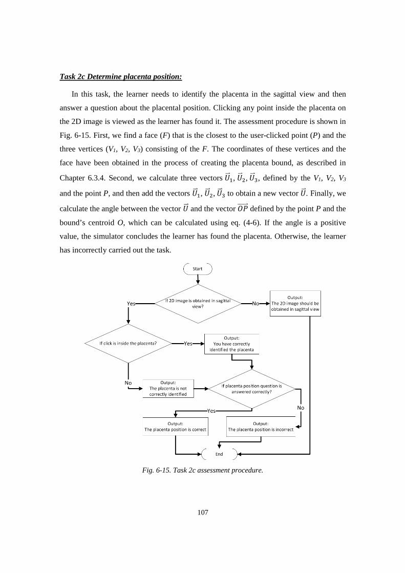
107

Task 2c Determine placenta position:

In this task, the learner needs to identify the placenta in the sagittal view and then

answer a question about the placental position. Clicking any point inside the placenta on

the 2D image is viewed as the learner has found it. The assessment procedure is shown in

Fig. 6-15. First, we find a face (F) that is the closest to the user-clicked point (P) and the

three vertices (V1, V2, V3) consisting of the F. The coordinates of these vertices and the

face have been obtained in the process of creating the placenta bound, as described in

Chapter 6.3.4. Second, we calculate three vectors êÄÄë�, êÄÄë�,êÄÄë�, defined by the V1, V2, V3

and the point P, and then add the vectors êÄÄë�, êÄÄë�,êÄÄë� to obtain a new vector êÄÄë. Finally, we

calculate the angle between the vector êÄÄë and the vector ¿âÄÄÄÄÄë defined by the point P and the

bound’s centroid O, which can be calculated using eq. (4-6). If the angle is a positive

value, the simulator concludes the learner has found the placenta. Otherwise, the learner

has incorrectly carried out the task.

Fig. 6-15. Task 2c assessment procedure.

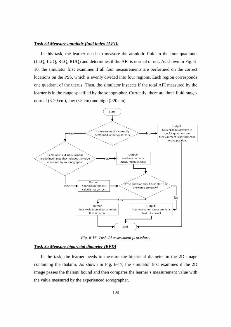
108

Task 2d Measure amniotic fluid index (AFI):

In this task, the learner needs to measure the amniotic fluid in the four quadrants

(LLQ, LUQ, RLQ, RUQ) and determines if the AFI is normal or not. As shown in Fig. 6-

16, the simulator first examines if all four measurements are performed on the correct

locations on the PSS, which is evenly divided into four regions. Each region corresponds

one quadrant of the uterus. Then, the simulator inspects if the total AFI measured by the

learner is in the range specified by the sonographer. Currently, there are three fluid ranges,

normal (8-20 cm), low (<8 cm) and high (>20 cm).

Fig. 6-16. Task 2d assessment procedure.

Task 3a Measure biparietal diameter (BPD)

In the task, the learner needs to measure the biparietal diameter in the 2D image

containing the thalami. As shown in Fig. 6-17, the simulator first examines if the 2D

image passes the thalami bound and then compares the learner’s measurement value with

the value measured by the experienced sonographer.

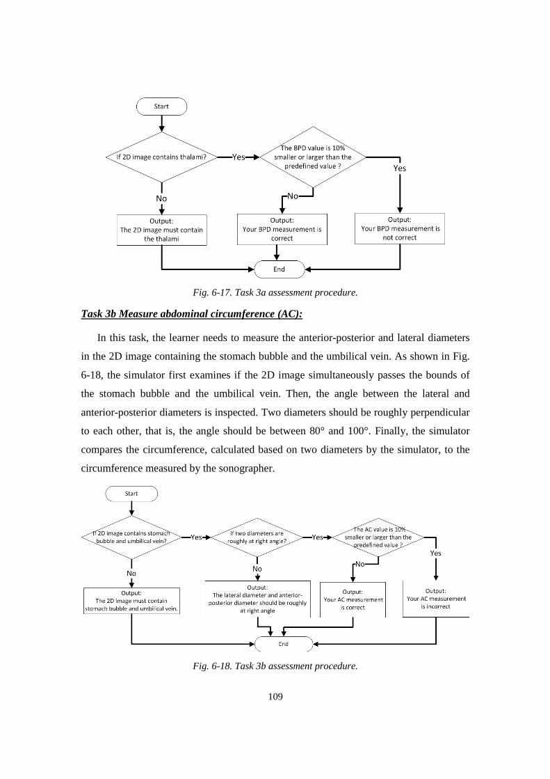
109

Fig. 6-17. Task 3a assessment procedure.

Task 3b Measure abdominal circumference (AC):

In this task, the learner needs to measure the anterior-posterior and lateral diameters

in the 2D image containing the stomach bubble and the umbilical vein. As shown in Fig.

6-18, the simulator first examines if the 2D image simultaneously passes the bounds of

the stomach bubble and the umbilical vein. Then, the angle between the lateral and

anterior-posterior diameters is inspected. Two diameters should be roughly perpendicular

to each other, that is, the angle should be between 80° and 100°. Finally, the simulator

compares the circumference, calculated based on two diameters by the simulator, to the

circumference measured by the sonographer.

Fig. 6-18. Task 3b assessment procedure.

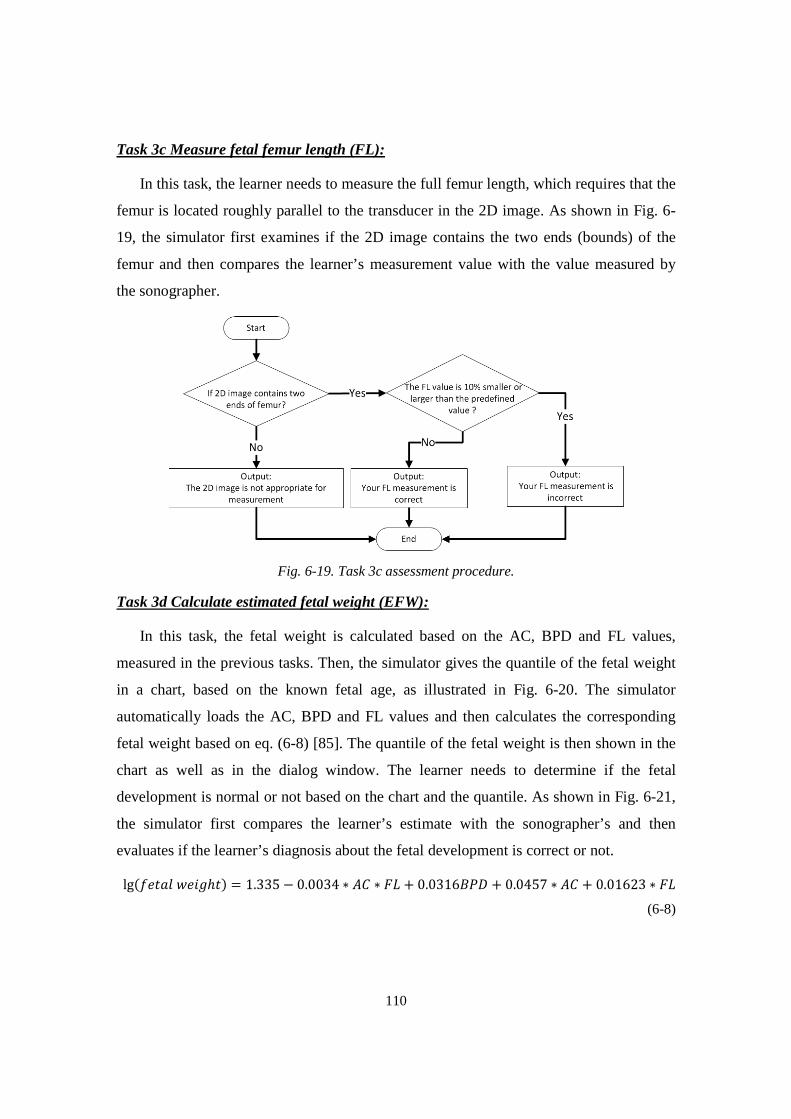
110

Task 3c Measure fetal femur length (FL):

In this task, the learner needs to measure the full femur length, which requires that the

femur is located roughly parallel to the transducer in the 2D image. As shown in Fig. 6-

19, the simulator first examines if the 2D image contains the two ends (bounds) of the

femur and then compares the learner’s measurement value with the value measured by

the sonographer.

Fig. 6-19. Task 3c assessment procedure.

Task 3d Calculate estimated fetal weight (EFW):

In this task, the fetal weight is calculated based on the AC, BPD and FL values,

measured in the previous tasks. Then, the simulator gives the quantile of the fetal weight

in a chart, based on the known fetal age, as illustrated in Fig. 6-20. The simulator

automatically loads the AC, BPD and FL values and then calculates the corresponding

fetal weight based on eq. (6-8) [85]. The quantile of the fetal weight is then shown in the

chart as well as in the dialog window. The learner needs to determine if the fetal

development is normal or not based on the chart and the quantile. As shown in Fig. 6-21,

the simulator first compares the learner’s estimate with the sonographer’s and then

evaluates if the learner’s diagnosis about the fetal development is correct or not.

lg(p3� *,3�Õℎ�) = 1.335 − 0.0034 ∗ ¹¾ ∗ ïY + 0.0316ñâò + 0.0457 ∗ ¹¾ + 0.01623 ∗ ïY

(6-8)

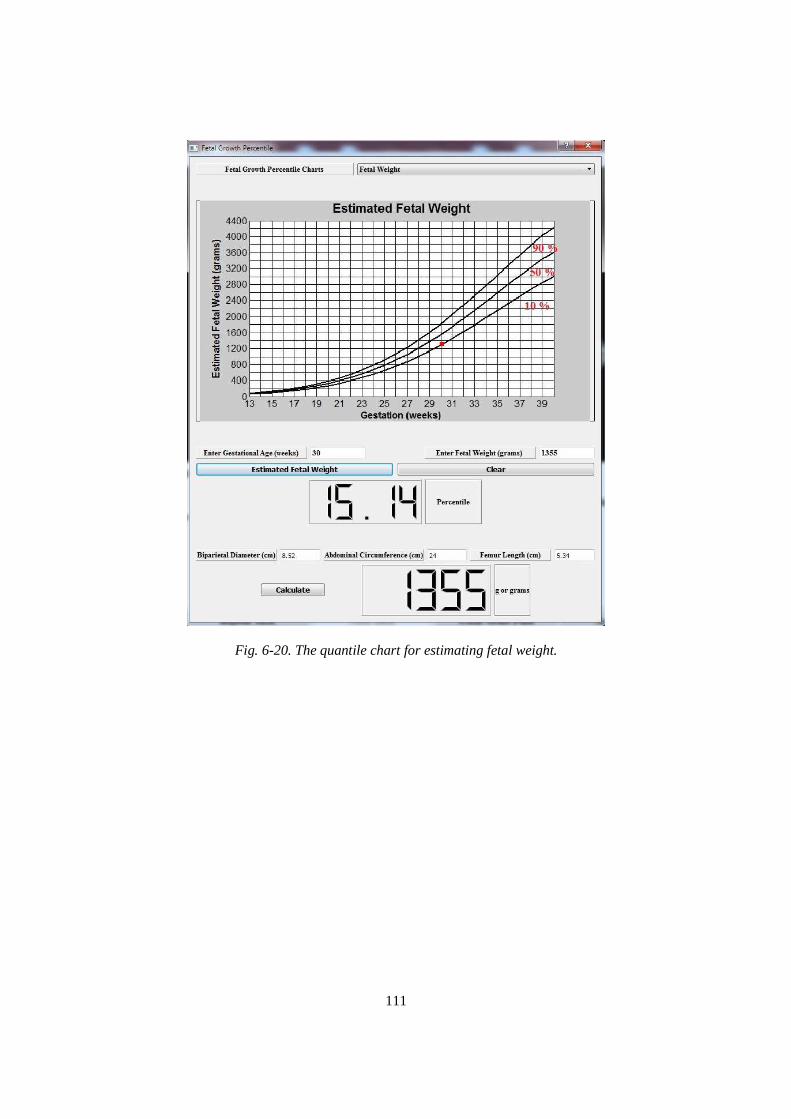
111

Fig. 6-20. The quantile chart for estimating fetal weight.

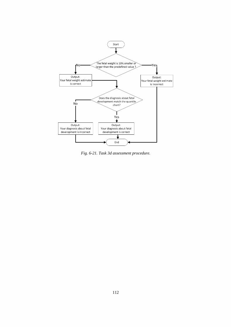
112

Fig. 6-21. Task 3d assessment procedure.

113

Chapter 7

Evaluation of the Training Simulator

In the previous chapters, we have described the design and implementation of an

affordable ultrasound simulator supporting freehand scan and self-paced obstetric

ultrasound training. In this chapter, we will first explain the goals and design of

evaluation experiments, where the simulator were evaluated based on two primary

qualities, the simulator performance and the training efficacy. Then, we will review the

experiment results regarding the 2D image quality, the rendering speed, the feasibility of

training tasks and assessment, and the training efficacy.

In the performance evaluation, the simulator was rated based on two qualities: i) an

adequate image generation and rendering speed for the simulator, and ii) a realistic 2D

ultrasound image quality and achievable biometric measurements. Additionally, we did a

preliminary experiment in which three sonographers evaluated the structured training

curriculum with the automatic assessment. These experiments were conducted before the

experiment that investigated the training efficacy so that we could understand the

simulator’s capability and feasibility of being used as a training tool.

To determine the training efficacy, the obstetric training simulator was evaluated by

24 3rd year medical students enrolled at UMASS Medical School in order to establish the

learning curve of the participants, specifically, the scan time of each training image

volume. The medical students were asked to practice ultrasound scan skills on six

training image volumes under the simulator’s guidance. An ideal experimental design

typically involves two groups, a control group and an experiment group, and the training

efficacy of the two groups is then compared. However, due to the constrained access to

114

UMASS medical students, we assigned all participants to the experiment group and

therefore there was no control group in our experiment. The training efficacy of the

simulator was indirectly determined from the learning curves of the participants.

7.1 Evaluation of the Simulator Performance

In this section, we first present the test results of the 2D image generation and the

rendering speed of the simulator on four different computers. Then, we compare 2D

ultrasound images generated from the simulator to actual ultrasound images acquired

from a pregnant subject at the same time that the 3D image volumes were acquired.

7.1.1 The simulator rendering speed

In the simulator design, the generation and the rendering speed of 2D images directly

impact the training experience and realism of the simulator. If the simulator cannot

generate and render 2D images with a satisfactory speed, the user will perceive frameskip,

i.e., the loss of 2D image frames. This issue is usually caused by insufficient hardware

processing capability and is a major root cause that makes the display of 2D images not

continuous on the simulator and degrades the training experience.

Our research had as one of its major objectives to design an affordable ultrasound

simulator. In addition to affordable scan tracking hardware, the simulator software should

be suitable for affordable computers. Thus, we have tested the simulator on four

moderately-priced computers with different hardware configurations, as described in

Table 7-1. All four computers had 64-bit Windows 7 installed and were compatible with

OpenGL 2.1 or onwards, as required by the VTK.

The processing speeds on the four computers were calculated in frames per sec (fps),

based on the total time of rendering 500 frames. The results are presented in Table 7-2.

These numbers also included the time required for rendering the virtual torso and the

virtual transducer. We configured the simulator to generate and render 2D images at a

speed of 33 fps, or process 2D images every 30 ms. Tables 7-1 and 7-2 indicate the

processing speed was largely dependent on the CPU, that is, a CPU having higher

frequency can process more 2D images in a unit time. A further test indicated that the

115

most intensive computation of the simulator is the tri-linear interpolation used in the 2D

image reslicer.

Table 7-1. The summary of the four computers used in the test.

The experiment results in Table 7-2 show that the simulator was able to generate and

render 2D images at a speed above 30 fps on the four computers. This met our design

goal of greater than 25 fps, which is a widely accepted requirement for smooth visual

presentation and minimum interfering motion blur or jitter. The CPU usage of the

simulator on Computers A, B and C typically ranged between 25% and 30%. The usage

occasionally went up to 40% in our test. The memory usage was roughly 600 MB on

Computers A, B, and C. The image volumes used for performance evaluation had an

average size of 800 by 550 by 900 voxels. The voxel resolution was 0.49 mm in the x, y

and z directions of 3D image volume coordinates.

Table 7-2. The rendering speed of 2D ultrasound images on laptops A, B, C and D.

Computer A B C D

Frame rate (fps) 45.66 39.37 35.39 30.60

Total (s) 10.95 12.70 14.13 16.34

7.1.2 Comparison between biometric measurements performed on and 2D images

obtained from the training simulator and a ultrasound machine

Given that biometric measurements are an important aspect of the obstetric

ultrasound training, we have compared the values of BPD, AC and FL measured on the

Computer CPU Supported Graphics Memory

A Xeon 3.2 GHz OpenGL 4.0 16 GB

B Core i7 2.9 GHz OpenGL 4.3 8 GB

C Core i5 2.5 GHz OpenGL 4.0 8 GB

D Core i3 2.3 GHz OpenGL 3.1 6 GB

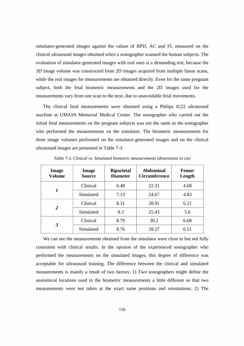
116

simulator-generated images against the values of BPD, AC and FL measured on the

clinical ultrasound images obtained when a sonographer scanned the human subjects. The

evaluation of simulator-generated images with real ones is a demanding test, because the

3D image volume was constructed from 2D images acquired from multiple linear scans,

while the real images for measurements are obtained directly. Even for the same pregnant

subject, both the fetal biometric measurements and the 2D images used for the

measurements vary from one scan to the next, due to unavoidable fetal movements.

The clinical fetal measurements were obtained using a Philips iU22 ultrasound

machine at UMASS Memorial Medical Center. The sonographer who carried out the

initial fetal measurements on the pregnant subjects was not the same as the sonographer

who performed the measurements on the simulator. The biometric measurements for

three image volumes performed on the simulator-generated images and on the clinical

ultrasound images are presented in Table 7-3.

Table 7-3. Clinical vs. Simulated biometric measurements (dimensions in cm)

Image Volume

Image Source

Biparietal Diameter

Abdominal Circumference

Femur Length

1 Clinical 6.48 22.31 4.68

Simulated 7.13 24.67 4.83

2 Clinical 8.31 28.91 6.21

Simulated 8.3 25.43 5.6

3 Clinical 8.79 30.2 6.68

Simulated 8.76 28.27 6.51

We can see the measurements obtained from the simulator were close to but not fully

consistent with clinical results. In the opinion of the experienced sonographer who

performed the measurements on the simulated images, this degree of difference was

acceptable for ultrasound training. The difference between the clinical and simulated

measurements is mainly a result of two factors: 1) Two sonographers might define the

anatomical locations used in the biometric measurements a little different so that two

measurements were not taken at the exact same positions and orientations. 2) The

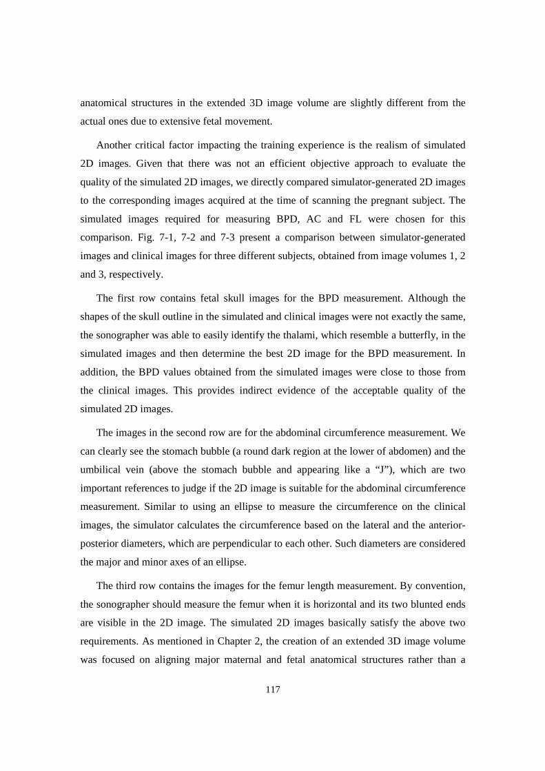
117

anatomical structures in the extended 3D image volume are slightly different from the

actual ones due to extensive fetal movement.

Another critical factor impacting the training experience is the realism of simulated

2D images. Given that there was not an efficient objective approach to evaluate the

quality of the simulated 2D images, we directly compared simulator-generated 2D images

to the corresponding images acquired at the time of scanning the pregnant subject. The

simulated images required for measuring BPD, AC and FL were chosen for this

comparison. Fig. 7-1, 7-2 and 7-3 present a comparison between simulator-generated

images and clinical images for three different subjects, obtained from image volumes 1, 2

and 3, respectively.

The first row contains fetal skull images for the BPD measurement. Although the

shapes of the skull outline in the simulated and clinical images were not exactly the same,

the sonographer was able to easily identify the thalami, which resemble a butterfly, in the

simulated images and then determine the best 2D image for the BPD measurement. In

addition, the BPD values obtained from the simulated images were close to those from

the clinical images. This provides indirect evidence of the acceptable quality of the

simulated 2D images.

The images in the second row are for the abdominal circumference measurement. We

can clearly see the stomach bubble (a round dark region at the lower of abdomen) and the

umbilical vein (above the stomach bubble and appearing like a “J”), which are two

important references to judge if the 2D image is suitable for the abdominal circumference

measurement. Similar to using an ellipse to measure the circumference on the clinical

images, the simulator calculates the circumference based on the lateral and the anterior-

posterior diameters, which are perpendicular to each other. Such diameters are considered

the major and minor axes of an ellipse.

The third row contains the images for the femur length measurement. By convention,

the sonographer should measure the femur when it is horizontal and its two blunted ends

are visible in the 2D image. The simulated 2D images basically satisfy the above two

requirements. As mentioned in Chapter 2, the creation of an extended 3D image volume

was focused on aligning major maternal and fetal anatomical structures rather than a

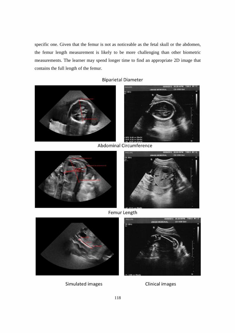
118

specific one. Given that the femur is not as noticeable as the fetal skull or the abdomen,

the femur length measurement is likely to be more challenging than other biometric

measurements. The learner may spend longer time to find an appropriate 2D image that

contains the full length of the femur.

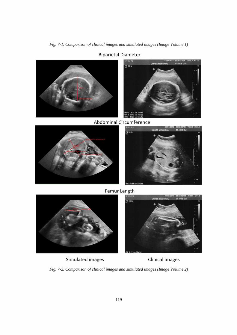
119

Fig. 7-1. Comparison of clinical images and simulated images (Image Volume 1)

Fig. 7-2. Comparison of clinical images and simulated images (Image Volume 2)

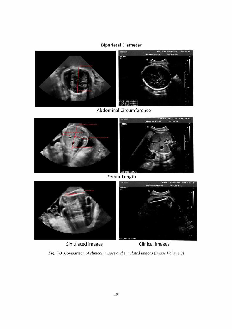
120

Fig. 7-3. Comparison of clinical images and simulated images (Image Volume 3)

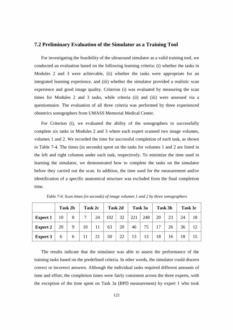
121

7.2 Preliminary Evaluation of the Simulator as a Training Tool

For investigating the feasibility of the ultrasound simulator as a valid training tool, we

conducted an evaluation based on the following learning criteria: (i) whether the tasks in

Modules 2 and 3 were achievable, (ii) whether the tasks were appropriate for an

integrated learning experience, and (iii) whether the simulator provided a realistic scan

experience and good image quality. Criterion (i) was evaluated by measuring the scan

times for Modules 2 and 3 tasks, while criteria (ii) and (iii) were assessed via a

questionnaire. The evaluation of all three criteria was performed by three experienced

obstetrics sonographers from UMASS Memorial Medical Center.

For Criterion (i), we evaluated the ability of the sonographers to successfully

complete six tasks in Modules 2 and 3 where each expert scanned two image volumes,

volumes 1 and 2. We recorded the time for successful completion of each task, as shown

in Table 7-4. The times (in seconds) spent on the tasks for volumes 1 and 2 are listed in

the left and right columns under each task, respectively. To minimize the time used in

learning the simulator, we demonstrated how to complete the tasks on the simulator

before they carried out the scan. In addition, the time used for the measurement and/or

identification of a specific anatomical structure was excluded from the final completion

time.

Table 7-4. Scan times (in seconds) of image volumes 1 and 2 by three sonographers

The results indicate that the simulator was able to assess the performance of the

training tasks based on the predefined criteria. In other words, the simulator could discern

correct or incorrect answers. Although the individual tasks required different amounts of

time and effort, the completion times were fairly consistent across the three experts, with

the exception of the time spent on Task 3a (BPD measurement) by expert 1 who took

Task 2b Task 2c Task 2d Task 3a Task 3b Task 3c

Expert 1 10 8 7 24 102 32 221 248 20 23 24 18

Expert 2 20 9 10 11 63 20 46 75 17 26 36 12

Expert 3 6 6 11 21 50 22 13 13 18 16 18 15

122

longer time, mainly because we defined a tight bound around the thalami, thus making

the criteria of selecting the appropriate 2D images for the measurement more strict.

From the responses in the questionnaire, all three sonographers agreed that the tasks

were easily performed and well organized in sequence. In addition, the sonographers

considered the simulated images to be adequately realistic for ultrasound training and

found the simulator to provide a fully adequate level of processing speed. They further

noted that the simulator had the potential for becoming a good supplemental training tool

for medical students and resident doctors and that the training tasks were appropriate for

obstetrics training.

One sonographer indicated that the absence of a beating fetal heart in the ultrasound

image of the simulator somewhat detracted from the realism. This is because the

sonographer usually first inspects the fetal heart at the beginning of obstetric ultrasound

examination and then performs the tasks defined in our training curriculum. In response

to this comment, we have now implemented the dynamic fetal heart on the simulator, as

described in Chapter 5.8.

7.3 Evaluation of the Simulator Training Efficacy

As stated in the previous section, the simulator has the potential of being a

supplementary obstetric ultrasound training tool for different groups of people, such as

medical students or residents. Accordingly, we designed a clinical study to investigate the

training efficacy of the simulator by three groups of medical students. In this section, we

will review the evaluation experiment and present the results. Following that, we will

summarize the data collected from the experiment and give a conclusion.

7.3.1 Design of the clinical evaluation

The role of an ultrasound simulator is to train and evaluate the psycho-motor skills

(hand-eye coordination, coupled with relevant anatomical knowledge), which is critical to

ultrasound scan proficiency and cannot be taught in a classroom setting. As we presented

in Chapter 1, the effectiveness of simulators in ultrasound education has been

documented through publications [33-46] in which the authors directly compared the

scan proficiency (the scan time and accuracy of biometric measurement) of two groups of

123

participants. One group received the training on ultrasound simulators whereas the other

group completed the training via traditional education.

The training efficacy evaluation was specifically designed for obstetric ultrasound,

based on a set of built-in training tasks following the basic AIUM protocol, except that

there was no control group. Thus, the training efficacy was indirectly evaluated by

comparing each individual’s scan proficiency as the student progressed through a set of

training image volumes. Specifically, the experiment evaluated how the simulator

facilitated the learning of basic ultrasound scan, by measuring how much faster and/or

more correctly scan tasks were performed on subsequent image volumes in a stipulated

sequence, relative to the initial image volume. In addition, each participating student was

asked, at the completion of all training image volumes, to complete a survey.

Our initial plan was to recruit 10 to 20 3rd or 4th year medical students from UMASS

Medical School, who were considering OB/GYN or Family Medicine as their specialty.

This is because 3rd or 4th year students have usually completed some necessary medical

courses, such as anatomy, physiology and pathology, and have no or little ultrasound

experience. All voluntary participants would not receive compensation for the experiment.

However, we failed to recruit a large enough number of participants for our experiment.

With the help of Dr. Michele Pugnaire at UMASS Medical School, the experiment was

integrated into the clerkship program of the Department of Obstetrics and Gynecology

(OB/GYN) of UMASS Memorial Medical Center. A total of 24 3rd year medical students

were recruited when they participated in a 5-week OB/GYN clerkship program.

7.3.2 Overview of the clinical evaluation

In this section, we will present the experiment details, including the selection of

training image volumes, experiment arrangement and data collection.

Image volume selection

As shown in Table 7-5, a total of 9 candidate training image volumes were generated.

However, not all of them proved suitable for the training. Dr. Petra Belady helped us with

selecting the best 6 image volumes for the experiment based on the 2D image quality of

each training task.

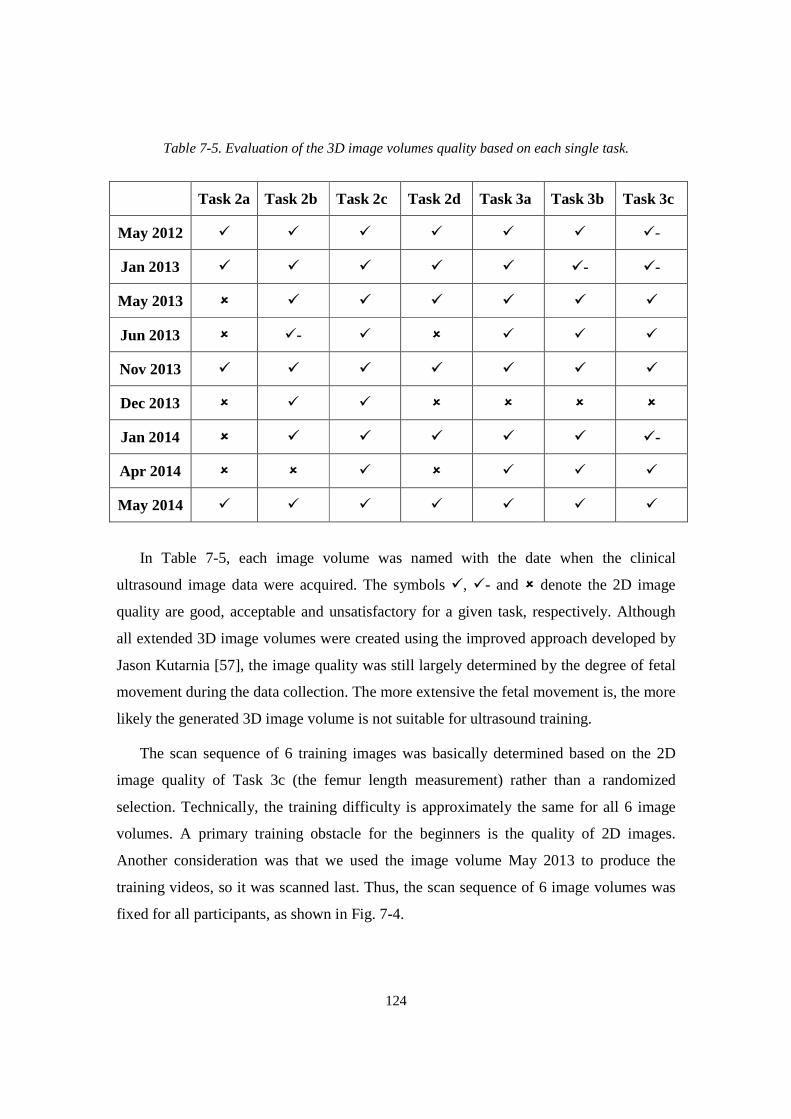
124

Table 7-5. Evaluation of the 3D image volumes quality based on each single task.

In Table 7-5, each image volume was named with the date when the clinical

ultrasound image data were acquired. The symbols �, �- and � denote the 2D image

quality are good, acceptable and unsatisfactory for a given task, respectively. Although

all extended 3D image volumes were created using the improved approach developed by

Jason Kutarnia [57], the image quality was still largely determined by the degree of fetal

movement during the data collection. The more extensive the fetal movement is, the more

likely the generated 3D image volume is not suitable for ultrasound training.

The scan sequence of 6 training images was basically determined based on the 2D

image quality of Task 3c (the femur length measurement) rather than a randomized

selection. Technically, the training difficulty is approximately the same for all 6 image

volumes. A primary training obstacle for the beginners is the quality of 2D images.

Another consideration was that we used the image volume May 2013 to produce the

training videos, so it was scanned last. Thus, the scan sequence of 6 image volumes was

fixed for all participants, as shown in Fig. 7-4.

Task 2a Task 2b Task 2c Task 2d Task 3a Task 3b Task 3c

May 2012 � � � � � � �-

Jan 2013 � � � � � �- �-

May 2013 � � � � � � �

Jun 2013 � �- � � � � �

Nov 2013 � � � � � � �

Dec 2013 � � � � � � �

Jan 2014 � � � � � � �-

Apr 2014 � � � � � � �

May 2014 � � � � � � �

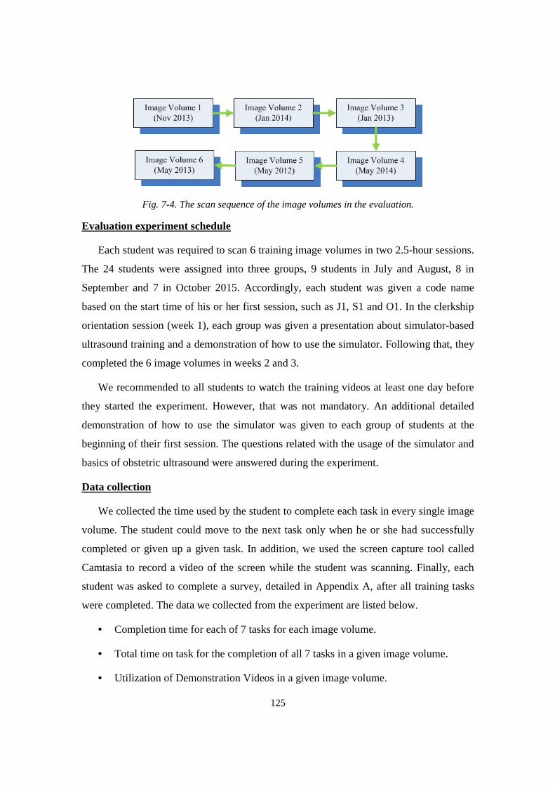
125

Fig. 7-4. The scan sequence of the image volumes in the evaluation.

Evaluation experiment schedule

Each student was required to scan 6 training image volumes in two 2.5-hour sessions.

The 24 students were assigned into three groups, 9 students in July and August, 8 in

September and 7 in October 2015. Accordingly, each student was given a code name

based on the start time of his or her first session, such as J1, S1 and O1. In the clerkship

orientation session (week 1), each group was given a presentation about simulator-based

ultrasound training and a demonstration of how to use the simulator. Following that, they

completed the 6 image volumes in weeks 2 and 3.

We recommended to all students to watch the training videos at least one day before

they started the experiment. However, that was not mandatory. An additional detailed

demonstration of how to use the simulator was given to each group of students at the

beginning of their first session. The questions related with the usage of the simulator and

basics of obstetric ultrasound were answered during the experiment.

Data collection

We collected the time used by the student to complete each task in every single image

volume. The student could move to the next task only when he or she had successfully

completed or given up a given task. In addition, we used the screen capture tool called

Camtasia to record a video of the screen while the student was scanning. Finally, each

student was asked to complete a survey, detailed in Appendix A, after all training tasks

were completed. The data we collected from the experiment are listed below.

• Completion time for each of 7 tasks for each image volume.

• Total time on task for the completion of all 7 tasks in a given image volume.

• Utilization of Demonstration Videos in a given image volume.

126

• Utilization of Help Functions (mainly in the form of help images) in a given

image volume.

• Scan pattern of the sham transducer, where we recorded the total length of the

scan path for each task.

• Video screen capture of the user interface on the computer screen, while the

student was scanning. No sound were recorded. No specific usage for this is

currently planned.

• Data from the survey.

7.3.3 Highlights of the survey feedback

The purpose of the survey was to provide additional data to qualitatively evaluate the

training efficacy of the simulator. We designed a total of 14 questions in the survey,

including 13 multiple choices and 1 open question. These questions asked the students to

assess the simulator in terms of ultrasound scan experience, 2D image quality, scan

assessment feedback as well as specific evaluation of each training task. In the following

paragraphs, we will presents some highlights of the survey results.

Question 1: Do you think that the 2D ultrasound images are realistic?

As shown in Fig. 7-5 left column, 95% of the participants agreed that the simulator

was able to provide acceptable level of or realistic 2D ultrasound images and it could be

used for ultrasound training. The realism of 2D images was also confirmed by the

experienced sonographers, as stated in Chapter 7.2.

Question 2: Do you think the simulator offers you realistic scan experience?

As shown in Fig. 7-5 right column, 91% of the participants agreed that the simulator

was able to provide acceptable level of or realistic scan experience and it could be used

for ultrasound training. The experienced sonographers reached a similar conclusion.

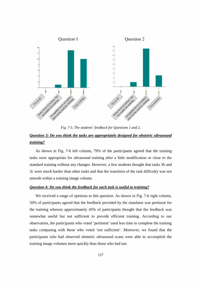
127

Fig. 7-5. The students’ feedback for Questions 1 and 2.

Question 3: Do you think the tasks are appropriately designed for obstetric ultrasound

training?

As shown in Fig. 7-6 left column, 79% of the participants agreed that the training

tasks were appropriate for ultrasound training after a little modification or close to the

standard training without any changes. However, a few students thought that tasks 3b and

3c were much harder than other tasks and that the transition of the task difficulty was not

smooth within a training image volume.

Question 4: Do you think the feedback for each task is useful to training?

We received a range of opinions to this question. As shown in Fig. 7-6 right column,

50% of participants agreed that the feedback provided by the simulator was pertinent for

the training whereas approximately 45% of participants thought that the feedback was

somewhat useful but not sufficient to provide efficient training. According to our

observation, the participants who voted ‘pertinent’ used less time to complete the training

tasks comparing with those who voted ‘not sufficient’. Moreover, we found that the

participants who had observed obstetric ultrasound scans were able to accomplish the

training image volumes more quickly than those who had not.

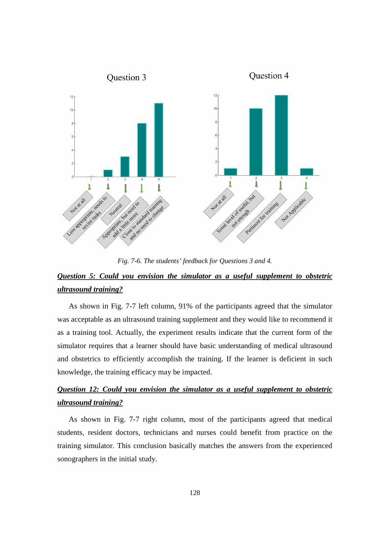
128

Fig. 7-6. The students’ feedback for Questions 3 and 4.

Question 5: Could you envision the simulator as a useful supplement to obstetric

ultrasound training?

As shown in Fig. 7-7 left column, 91% of the participants agreed that the simulator

was acceptable as an ultrasound training supplement and they would like to recommend it

as a training tool. Actually, the experiment results indicate that the current form of the

simulator requires that a learner should have basic understanding of medical ultrasound

and obstetrics to efficiently accomplish the training. If the learner is deficient in such

knowledge, the training efficacy may be impacted.

Question 12: Could you envision the simulator as a useful supplement to obstetric

ultrasound training?

As shown in Fig. 7-7 right column, most of the participants agreed that medical

students, resident doctors, technicians and nurses could benefit from practice on the

training simulator. This conclusion basically matches the answers from the experienced

sonographers in the initial study.

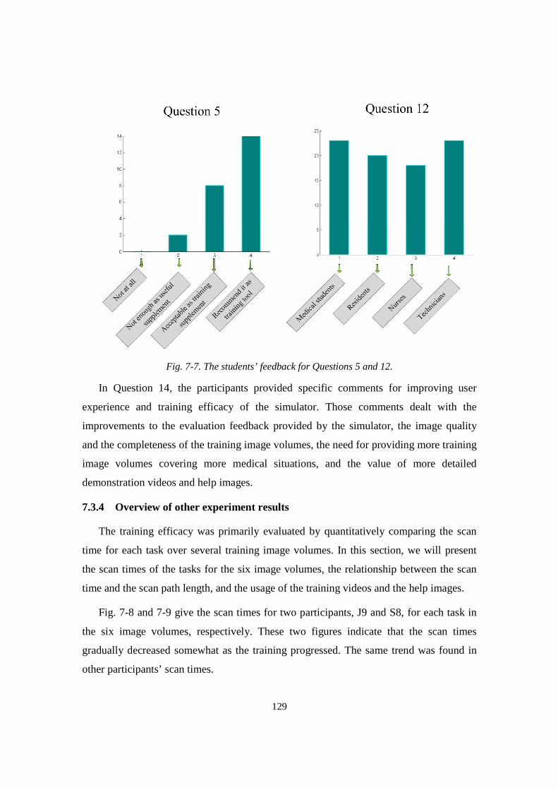
129

Fig. 7-7. The students’ feedback for Questions 5 and 12.

In Question 14, the participants provided specific comments for improving user

experience and training efficacy of the simulator. Those comments dealt with the

improvements to the evaluation feedback provided by the simulator, the image quality

and the completeness of the training image volumes, the need for providing more training

image volumes covering more medical situations, and the value of more detailed

demonstration videos and help images.

7.3.4 Overview of other experiment results

The training efficacy was primarily evaluated by quantitatively comparing the scan

time for each task over several training image volumes. In this section, we will present

the scan times of the tasks for the six image volumes, the relationship between the scan

time and the scan path length, and the usage of the training videos and the help images.

Fig. 7-8 and 7-9 give the scan times for two participants, J9 and S8, for each task in

the six image volumes, respectively. These two figures indicate that the scan times

gradually decreased somewhat as the training progressed. The same trend was found in

other participants’ scan times.

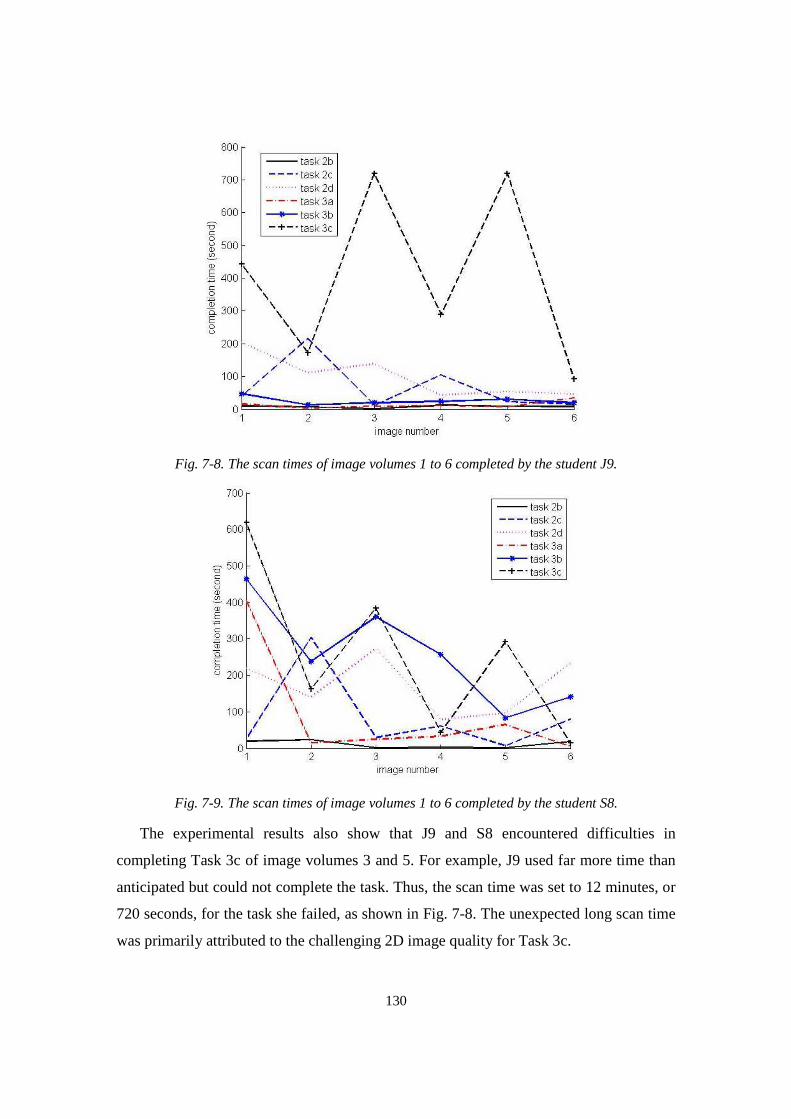
130

Fig. 7-8. The scan times of image volumes 1 to 6 completed by the student J9.

Fig. 7-9. The scan times of image volumes 1 to 6 completed by the student S8.

The experimental results also show that J9 and S8 encountered difficulties in

completing Task 3c of image volumes 3 and 5. For example, J9 used far more time than

anticipated but could not complete the task. Thus, the scan time was set to 12 minutes, or

720 seconds, for the task she failed, as shown in Fig. 7-8. The unexpected long scan time

was primarily attributed to the challenging 2D image quality for Task 3c.

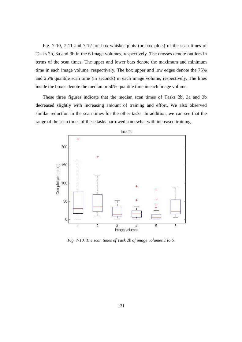
131

Fig. 7-10, 7-11 and 7-12 are box-whisker plots (or box plots) of the scan times of

Tasks 2b, 3a and 3b in the 6 image volumes, respectively. The crosses denote outliers in

terms of the scan times. The upper and lower bars denote the maximum and minimum

time in each image volume, respectively. The box upper and low edges denote the 75%

and 25% quantile scan time (in seconds) in each image volume, respectively. The lines

inside the boxes denote the median or 50% quantile time in each image volume.

These three figures indicate that the median scan times of Tasks 2b, 3a and 3b

decreased slightly with increasing amount of training and effort. We also observed

similar reduction in the scan times for the other tasks. In addition, we can see that the

range of the scan times of these tasks narrowed somewhat with increased training.

Fig. 7-10. The scan times of Task 2b of image volumes 1 to 6.

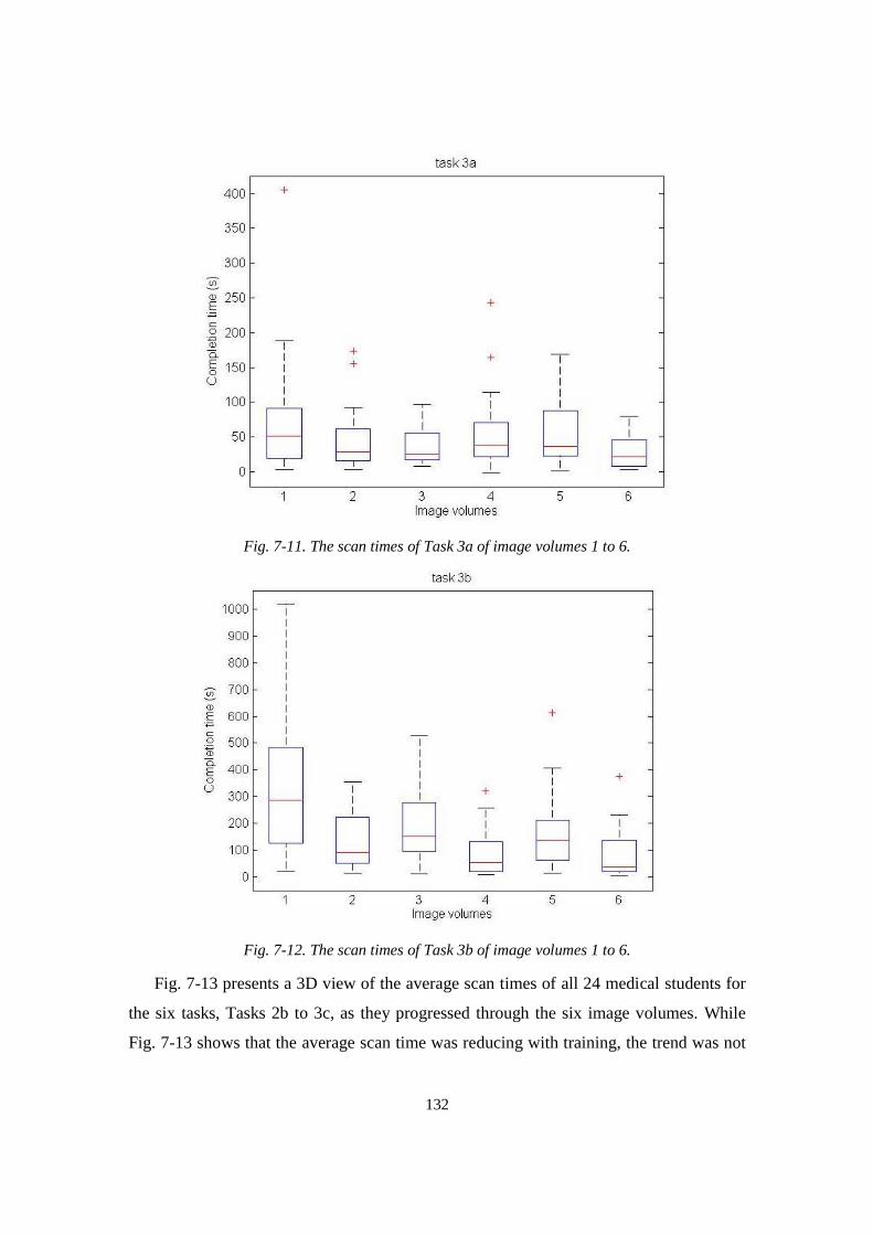
132

Fig. 7-11. The scan times of Task 3a of image volumes 1 to 6.

Fig. 7-12. The scan times of Task 3b of image volumes 1 to 6.

Fig. 7-13 presents a 3D view of the average scan times of all 24 medical students for

the six tasks, Tasks 2b to 3c, as they progressed through the six image volumes. While

Fig. 7-13 shows that the average scan time was reducing with training, the trend was not

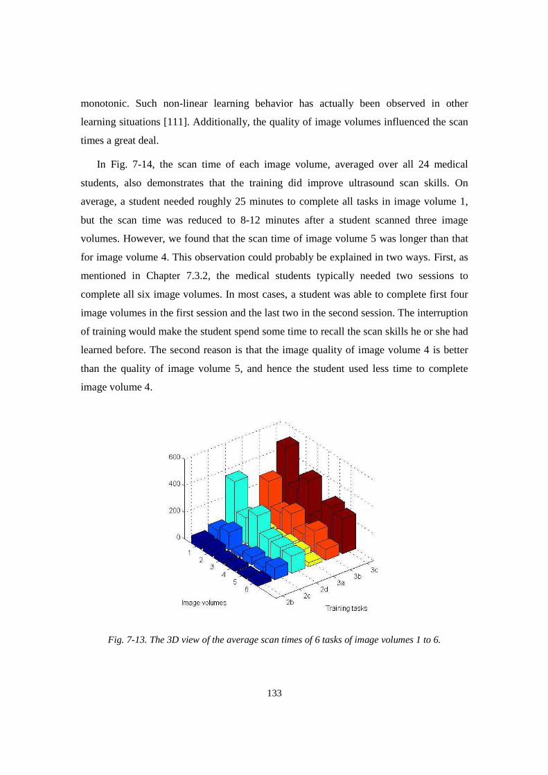
133

monotonic. Such non-linear learning behavior has actually been observed in other

learning situations [111]. Additionally, the quality of image volumes influenced the scan

times a great deal.

In Fig. 7-14, the scan time of each image volume, averaged over all 24 medical

students, also demonstrates that the training did improve ultrasound scan skills. On

average, a student needed roughly 25 minutes to complete all tasks in image volume 1,

but the scan time was reduced to 8-12 minutes after a student scanned three image

volumes. However, we found that the scan time of image volume 5 was longer than that

for image volume 4. This observation could probably be explained in two ways. First, as

mentioned in Chapter 7.3.2, the medical students typically needed two sessions to

complete all six image volumes. In most cases, a student was able to complete first four

image volumes in the first session and the last two in the second session. The interruption

of training would make the student spend some time to recall the scan skills he or she had

learned before. The second reason is that the image quality of image volume 4 is better

than the quality of image volume 5, and hence the student used less time to complete

image volume 4.

Fig. 7-13. The 3D view of the average scan times of 6 tasks of image volumes 1 to 6.

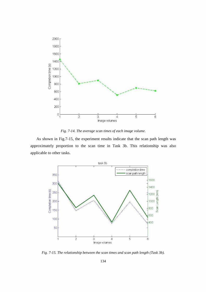
134

Fig. 7-14. The average scan times of each image volume.

As shown in Fig.7-15, the experiment results indicate that the scan path length was

approximately proportion to the scan time in Task 3b. This relationship was also

applicable to other tasks.

Fig. 7-15. The relationship between the scan times and scan path length (Task 3b).

135

Although we had encouraged all students to watch the training videos before the

experiment, about half of them did not do that. The training videos were rarely used

during the training and mostly watched during the tasks for the first image volume.

According to the experimental results, the video of measuring femur length was the most

watched video during the training. The videos of measuring abdominal circumference

and measuring amniotic fluid were the second and third most watched videos.

In addition to the training videos, the simulator also provided the medical students

with a set of help images for all image volumes except for the last one. Those help

images allowed the students to glance at the 2D images containing desired anatomical

structures. The experimental results show that a few students frequently used the help

images to complete the training tasks whereas other students used the help images only

when they had scanned a long time but had not found the correct answers. Analyzing the

usage of the helps images revealed that the participants utilized the help images mostly in

Task 3c, followed by Task 3b and Task 2d. Actually, the inclination of using the help

images during the training was directly related with the scan time. If the participant could

not find the correct answer after practicing for a certain amount of time, he or she was

more likely to resort external help.

7.3.5 Summary of the clinical evaluation

Based on the experiment results, we observed that the successful completion time of

each task gradually decreased with the training. This provides some level of evidence of

the training efficacy of the simulator. Moreover, some of the students confirmed that the

training on the simulator facilitated their learning of obstetric ultrasound during the

clerkship program. Although the completion time was also influenced by the image

quality of the tasks, which varies with image volumes, it does not invalidate such a

conclusion. The experimental result also indicates that the scan length was approximately

proportion to the completion time.

The survey completed by all 24 students shows that the simulator provided a useful

level of ultrasound scan experience, that the quality of the ultrasound images was

acceptable and that the simulator had the potential of becoming a valuable supplemental

tool for obstetric ultrasound training. Their feedback was consistent with that obtained

136

from the experienced sonographers in the preliminary experiment at UMASS Memorial

Medical Center. In addition, some students reported that the level of difficulty for the six

tasks varied significantly within one image volume. For example, Task 2b and 2c were

much easier than the rest. Almost all 24 students agreed that the simulator might be a

suitable training tool for medical students, resident doctors, nurses and technicians.

Utilizing the students’ feedback, there are a few improvements that should be

implemented in a future version of the simulator to make the training more efficiently and

suitable for medical students. These improvements include: 1) providing more task

assessment feedback to the learner; 2) providing more training cases (image volumes)

that cover more medical conditions; 3) improving the 2D image quality and completeness.

137

Chapter 8

The Ultrasound E-training based on the Networked

Simulators

In the past decade, with the evolution of internet technology, distance education has

become more widely used. According to a report from the National Center for Education

Statistics [112], 22 % of graduates and 11 % of undergraduates enrolled in distance

education programs in 2012, and the number of enrollments had been growing over the

last ten years. While distance education does require a greater amount of self-discipline,

an instructor still plays a significant role. In a typical case, a student can take online

classes and quizzes on a flexible basis, according to his or her schedule, but the student

must complete these classes and quizzes within a certain time frame. The instructor is

also able to request a group learning session and can ask all or a part of students to

remotely join the session at a specific time.

Distance education applied to ultrasound training can be divided into two separate

categories: E-learning in didactic ultrasound and E-training (remote training) in

ultrasound scan. The didactic ultrasound is focused on basic ultrasound physics, human

anatomy, physiology, pathology, etc., and can be acquired through traditional classroom

courses, through self-study or through on-line courses. The E-learning material is mainly

delivered in the form of texts, audios, animations, streaming videos via internet, CDs and

DVDs, eliminating the need for classrooms and making the training more affordable and

flexible. In most of cases, the courses are delivered through pre-recorded videos or text-

based reading materials. In contrast, the ultrasound hands-on training is focused on the

138

learning of ultrasound scan skills on actual subjects by observing the instructor’s

demonstration and practicing the skills under the instructor’s guidance.

The E-learning in didactic ultrasound has been reported in a few published papers

[21,113,114] and all of them have reached a similar conclusion that the E-learning can

efficiently deliver the didactic ultrasound training. However, current E-learning systems

for didactic ultrasound cannot provide scan training, or ultrasound E-training, which

requires that all participating students can learn and practice ultrasound scan under the

guidance of an instructor at different locations.

As of now, only a few attempts of delivering ultrasound E-training have been

reported. VSee Telemedicine [115] has developed hardware that can be integrated to a

regular ultrasound machine. With this hardware, a doctor can observe ultrasound scan

remotely performed by another doctor. Through a video stream, doctors in rural areas can

remotely receive instructions, such as how to appropriately use the probe. However, one

noticeable problem of this system for ultrasound training is that video plus voice

transmission may not be feasible in regions only having limited speed networks. In

addition, this system must be installed on an existing ultrasound system and not suitable

for multiple learners. In another recent study, Cenydd [116] built a remote ultrasound

training mentor system based on the Wii technology. Although the system is not

expensive, their simulator has a few limitations, such as 1) the 2D images are generated

based on CT-based images; 2) the simulator provides non-realistic ultrasound scan; 3) the

system serves as only a monitor rather than a training system.

This chapter describes an inexpensive, compact ultrasound E-training system utilizing

the ultrasound obstetric simulator, described in the previous chapters. The E-training

system consists of a dedicated server and multiple network-connected simulators (one

simulator for each user) that can be located at multiple sites. The system provides

synchronous and asynchronous training modes. The synchronous (or group-learning)

mode allows all training participants to observe the scan ability of a chosen learner, or a

demonstration by the instructor, in real-time with a low transmission bit rate. This is

achieved by directly transmitting position and orientation data from the sham transducer,

rather than 2D ultrasound images, and resulting in a system performance independent of

139

network bandwidth. The asynchronous mode was actually implemented with the training

approach described in Chapter 6.

8.1 Implementation of E-training System

The complete E-training system is composed of the networked simulators and a

dedicated server, as shown in Fig. 8-1. As described in the previous chapters, a key factor

to simulate realistic obstetric ultrasound scan is that the simulator should be able to

mimic freehand scan on the abdominal surface of a pregnant woman. Accordingly, all

networked simulators should be able, on their own screens, to synchronously display the

same movement of the virtual transducer on the virtual torso and display the same 2D

ultrasound image. In other words, all networked simulators except one work as passive

monitors, displaying the same 2D ultrasound image, virtual transducer etc., as on the

active simulator, on which a user performs ultrasound scan. The passive and active

simulators are referred to as the observer simulator and the operator simulator,

respectively. To achieve this in a traditional design, an E-training system has to directly

transmit the 2D images. Although real-time video streaming is technically feasible over

high speed internets, such as broadband networks or 4G mobile networks in the United

States or other developed countries, real-time video streaming over 2G/3G mobile or low

speed networks is still a challenge. Such limited speed networks are often encountered in

developing countries.

An alternative to resolving this problem is to only transmit the sham transducer’s

position and orientation (the five degree of freedom data described in Chapter 3), so that

the data transmission only requires a very low bit rate. This requires that all participants

must have the same image volume loaded, which is ensured through software commands

from the instructor.

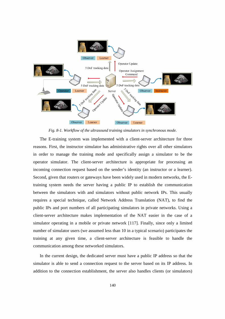
140

Fig. 8-1. Workflow of the ultrasound training simulators in synchronous mode.

The E-training system was implemented with a client-server architecture for three

reasons. First, the instructor simulator has administrative rights over all other simulators

in order to manage the training mode and specifically assign a simulator to be the

operator simulator. The client-server architecture is appropriate for processing an

incoming connection request based on the sender’s identity (an instructor or a learner).

Second, given that routers or gateways have been widely used in modern networks, the E-

training system needs the server having a public IP to establish the communication

between the simulators with and simulators without public network IPs. This usually

requires a special technique, called Network Address Translation (NAT), to find the

public IPs and port numbers of all participating simulators in private networks. Using a

client-server architecture makes implementation of the NAT easier in the case of a

simulator operating in a mobile or private network [117]. Finally, since only a limited

number of simulator users (we assumed less than 10 in a typical scenario) participates the

training at any given time, a client-server architecture is feasible to handle the

communication among these networked simulators.

In the current design, the dedicated server must have a public IP address so that the

simulator is able to send a connection request to the server based on its IP address. In

addition to the connection establishment, the server also handles clients (or simulators)

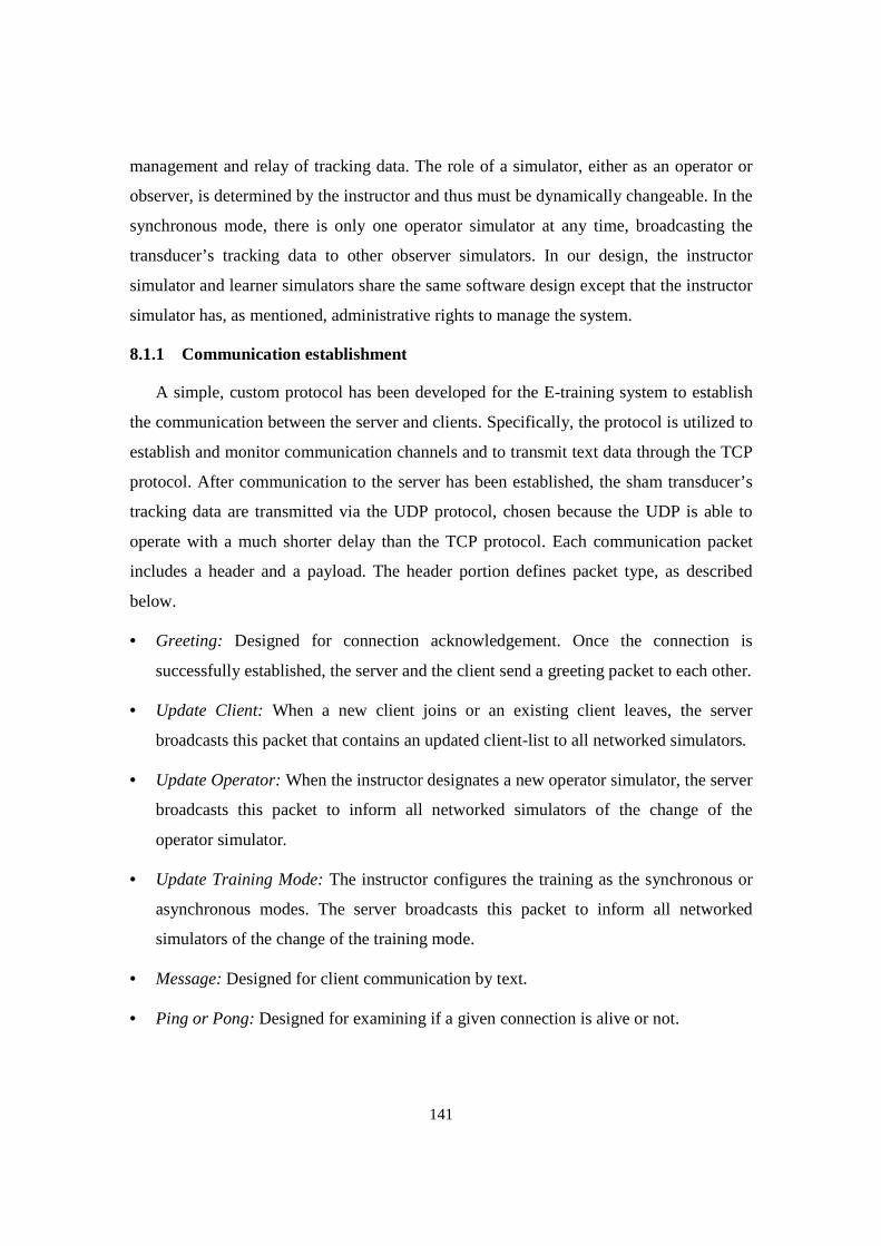
141

management and relay of tracking data. The role of a simulator, either as an operator or

observer, is determined by the instructor and thus must be dynamically changeable. In the

synchronous mode, there is only one operator simulator at any time, broadcasting the

transducer’s tracking data to other observer simulators. In our design, the instructor

simulator and learner simulators share the same software design except that the instructor

simulator has, as mentioned, administrative rights to manage the system.

8.1.1 Communication establishment

A simple, custom protocol has been developed for the E-training system to establish

the communication between the server and clients. Specifically, the protocol is utilized to

establish and monitor communication channels and to transmit text data through the TCP

protocol. After communication to the server has been established, the sham transducer’s

tracking data are transmitted via the UDP protocol, chosen because the UDP is able to

operate with a much shorter delay than the TCP protocol. Each communication packet

includes a header and a payload. The header portion defines packet type, as described

below.

• Greeting: Designed for connection acknowledgement. Once the connection is

successfully established, the server and the client send a greeting packet to each other.

• Update Client: When a new client joins or an existing client leaves, the server

broadcasts this packet that contains an updated client-list to all networked simulators.

• Update Operator: When the instructor designates a new operator simulator, the server

broadcasts this packet to inform all networked simulators of the change of the

operator simulator.

• Update Training Mode: The instructor configures the training as the synchronous or

asynchronous modes. The server broadcasts this packet to inform all networked

simulators of the change of the training mode.

• Message: Designed for client communication by text.

• Ping or Pong: Designed for examining if a given connection is alive or not.

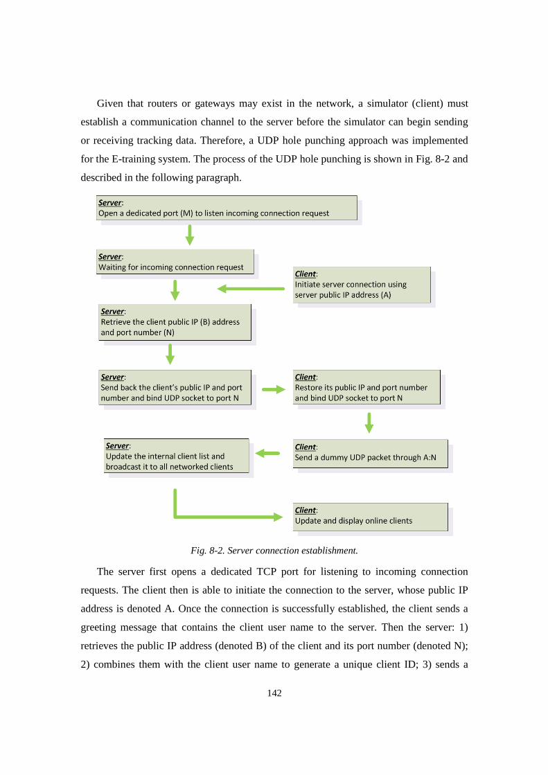
142

Given that routers or gateways may exist in the network, a simulator (client) must

establish a communication channel to the server before the simulator can begin sending

or receiving tracking data. Therefore, a UDP hole punching approach was implemented

for the E-training system. The process of the UDP hole punching is shown in Fig. 8-2 and

described in the following paragraph.

Fig. 8-2. Server connection establishment.

The server first opens a dedicated TCP port for listening to incoming connection

requests. The client then is able to initiate the connection to the server, whose public IP

address is denoted A. Once the connection is successfully established, the client sends a

greeting message that contains the client user name to the server. Then the server: 1)

retrieves the public IP address (denoted B) of the client and its port number (denoted N);

2) combines them with the client user name to generate a unique client ID; 3) sends a

143

greeting message that contains the IP address and port information (B:N) back to the

client; and 4) binds a UDP socket to port N. After receiving the greeting message from

the server, the client sends a UDP packet to the address of A:N to make itself visible to

the server in the case that the simulator runs in a private network. Finally, the server

updates its client list and broadcasts the list to all networked simulators.

8.1.2 Data transmission

After the communication channel has been established, the operator simulator now

can send the transducer’s tracking data to the server through the “punched” UDP port.

The server then relays the tracking data to all observer simulators by searching a client

table, which will be updated when a client joins or leaves the session. At the client side, a

first-in-first-out buffer is used to queue the incoming tracking data so that the observer

simulator is able to smoothly render 2D images. If the buffer is full when new data arrive,

the simulator will decimate the tracking data in the buffer to make the buffer up-to-date.

If the buffer is empty, the simulator will use the immediate past tracking data to render

2D images.

In addition to the tracking data, the system also establishes text channels among all

clients by using the “Message” packet. Given that texts do not need to be synchronized,

the system transmits them through the TCP protocol.

8.1.3 Management of the operator simulator

In the synchronous mode, only one operator simulator is performing the scan while

all the other simulators are observers. The assignment of the operator simulator status is

managed by the instructor who can dynamically change the role of any simulator from an

observer to an operator or vice versa by sending an “update operator” packet to the server.

A string variable at the server side stores the ID of the operator simulator. Then, the

server informs all networked simulators of the change of the operator status. If the

instructor does not appoint any simulator to be the operator simulator, then all simulators

function as observers by default. It should be noted that the text channels are still

available in this mode.

144

8.2 Performance Evaluation of the E-training System

The performance evaluation of the E-training system was focused on the quality of

the transmitted tracking data by measuring latency, data loss and bit rate in the

transmission. The quality and rendering speed of the 2D ultrasound images for an

individual simulator have been detailed in Chapter 7. In this section, we first explain the

experimental conditions, then we present the results of transmission latency, data loss and

bit rate under a set of defined test conditions.

8.2.1 Experiment design of the E-training system

The E-training system is intended to work in two major types of networks, i.e.,

cellular networks or 802.11 wireless networks. Currently, major wireless carriers in the

United States have upgraded their cellular networks to 3G/4G. Accordingly, we have

only been able to test our system in 3G/4G networks. The carrier’s channel access

technology was not considered in our evaluation. For 802.11 wireless networks, the most

common scenario is that an end-user accesses the internet through a router at his/her

home, clinic or office; hence, we have only tested the system in a router-based wireless

network. The current E-training system was designed to support a limited number of

users in a given training session, and we tested it with the minimum number of

participants, specifically three simulators (one instructor and two learner simulators),

under the following three conditions.

A. All simulators in wireless networks.

B. All simulators in cellular networks.

C. Same condition as A, except that the data from the operator simulator were routed

via a laptop computer located in China.

The above three conditions covered most of cases where the system would be

operating. Condition C was intended to simulate the case where international learners

participate in the training. The test in each condition lasted 3 to 5 minutes. The hardware

configurations of the three computers running the three simulators are described in Table

8-1. All three computers had 64-bit Windows 7 and Intel HD graphic cards installed.

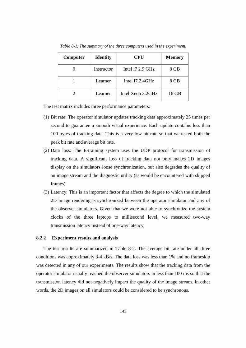
145

Table 8-1. The summary of the three computers used in the experiment.

Computer Identity CPU Memory

0 Instructor Intel i7 2.9 GHz 8 GB

1 Learner Intel i7 2.4GHz 8 GB

2 Learner Intel Xeon 3.2GHz 16 GB

The test matrix includes three performance parameters:

(1) Bit rate: The operator simulator updates tracking data approximately 25 times per

second to guarantee a smooth visual experience. Each update contains less than

100 bytes of tracking data. This is a very low bit rate so that we tested both the

peak bit rate and average bit rate.

(2) Data loss: The E-training system uses the UDP protocol for transmission of

tracking data. A significant loss of tracking data not only makes 2D images

display on the simulators loose synchronization, but also degrades the quality of

an image stream and the diagnostic utility (as would be encountered with skipped

frames).

(3) Latency: This is an important factor that affects the degree to which the simulated

2D image rendering is synchronized between the operator simulator and any of

the observer simulators. Given that we were not able to synchronize the system

clocks of the three laptops to millisecond level, we measured two-way

transmission latency instead of one-way latency.

8.2.2 Experiment results and analysis

The test results are summarized in Table 8-2. The average bit rate under all three

conditions was approximately 3-4 kB/s. The data loss was less than 1% and no frameskip

was detected in any of our experiments. The results show that the tracking data from the

operator simulator usually reached the observer simulators in less than 100 ms so that the

transmission latency did not negatively impact the quality of the image stream. In other

words, the 2D images on all simulators could be considered to be synchronous.

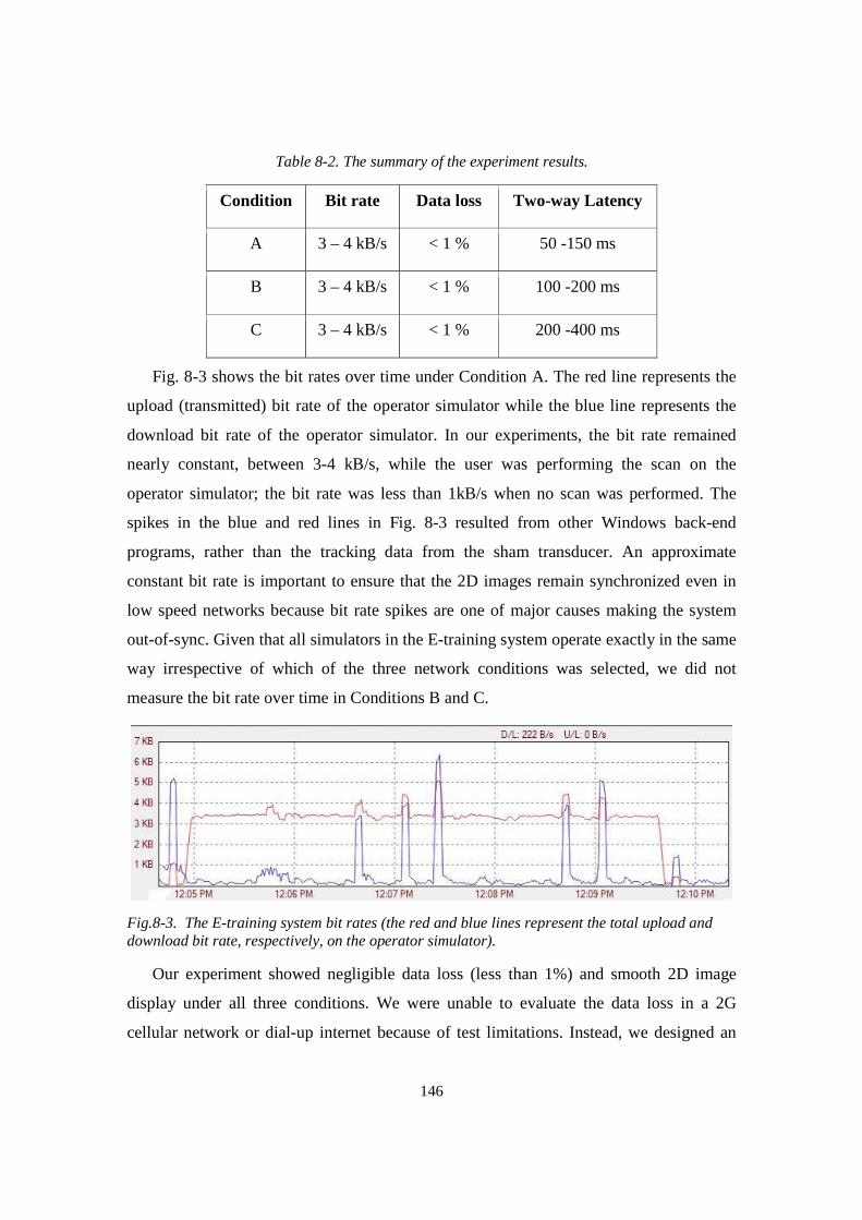
146

Table 8-2. The summary of the experiment results.

Condition Bit rate Data loss Two-way Latency

A 3 – 4 kB/s < 1 % 50 -150 ms

B 3 – 4 kB/s < 1 % 100 -200 ms

C 3 – 4 kB/s < 1 % 200 -400 ms

Fig. 8-3 shows the bit rates over time under Condition A. The red line represents the

upload (transmitted) bit rate of the operator simulator while the blue line represents the

download bit rate of the operator simulator. In our experiments, the bit rate remained

nearly constant, between 3-4 kB/s, while the user was performing the scan on the

operator simulator; the bit rate was less than 1kB/s when no scan was performed. The

spikes in the blue and red lines in Fig. 8-3 resulted from other Windows back-end

programs, rather than the tracking data from the sham transducer. An approximate

constant bit rate is important to ensure that the 2D images remain synchronized even in

low speed networks because bit rate spikes are one of major causes making the system

out-of-sync. Given that all simulators in the E-training system operate exactly in the same

way irrespective of which of the three network conditions was selected, we did not

measure the bit rate over time in Conditions B and C.

Fig.8-3. The E-training system bit rates (the red and blue lines represent the total upload and download bit rate, respectively, on the operator simulator).

Our experiment showed negligible data loss (less than 1%) and smooth 2D image

display under all three conditions. We were unable to evaluate the data loss in a 2G

cellular network or dial-up internet because of test limitations. Instead, we designed an

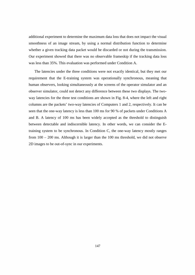
147

additional experiment to determine the maximum data loss that does not impact the visual

smoothness of an image stream, by using a normal distribution function to determine

whether a given tracking data packet would be discarded or not during the transmission.

Our experiment showed that there was no observable frameskip if the tracking data loss

was less than 35%. This evaluation was performed under Condition A.

The latencies under the three conditions were not exactly identical, but they met our

requirement that the E-training system was operationally synchronous, meaning that

human observers, looking simultaneously at the screens of the operator simulator and an

observer simulator, could not detect any difference between these two displays. The two-

way latencies for the three test conditions are shown in Fig. 8-4, where the left and right

columns are the packets’ two-way latencies of Computers 1 and 2, respectively. It can be

seen that the one-way latency is less than 100 ms for 90 % of packets under Conditions A

and B. A latency of 100 ms has been widely accepted as the threshold to distinguish

between detectable and indiscernible latency. In other words, we can consider the E-

training system to be synchronous. In Condition C, the one-way latency mostly ranges

from 100 – 200 ms. Although it is larger than the 100 ms threshold, we did not observe

2D images to be out-of-sync in our experiments.

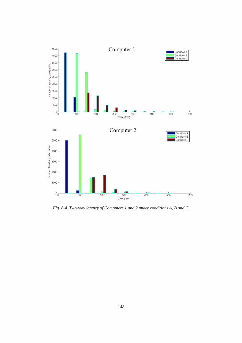
148

Fig. 8-4. Two-way latency of Computers 1 and 2 under conditions A, B and C.

149

Chapter 9

Conclusions and Future Improvements

9.1 The Dissertation Conclusions

In this dissertation, we have described a new low-cost, portable obstetric ultrasound

simulator providing realistic scan experience. The low-cost aspect dictates the design of

the 5 DoF tracking system, a requirement met by using an Anoto pen and a printed

surface for position tracking and an IMU for orientation tracking. The component cost of

the IMU, the Anoto pen, the physical scan surface and the transducer shell totals less than

$300. Making the simulator affordable also requires that the simulator software is able to

run on an ordinary computer. The module-based software design makes the simulator

able to run with a frame rate better than 25 fps. The realistic scan experience is made

possible by using training materials in the form of large, composite ultrasound image

volumes, with the realism further enhanced by incorporating a beating fetal heart. The

physical scan surface makes the scan experience realistic, that is, the learner can

continuously scan an extended region while allowing angling and rotation of the sham

transducer. This feature is critical to proper training in psychomotor skills.

The simulator is designed to provide simulator-assisted training on the basic or even

the intermediate obstetric ultrasound level, by integrating the training guidance and the

scan evaluation in the simulator software. We have formulated the training tasks and the

assessment criteria based on the AIUM’s standard practice of obstetric ultrasound.

Specifically, the structured training tasks aim to train a learner in the proper obstetric

ultrasound examination sequence, identification of critical anatomical structures and

biometric measurement. This is achieved by inserting landmark bounds for all anatomical

150

structures to be identified, either implemented with the algorithms or under the guidance

of obstetric sonographers.

A preliminary evaluation was performed by a group of three experienced

sonographers. They completed six specified tasks in a reasonable time by following the

instructions provided by the simulator. All three sonographers agreed that the training

tasks were appropriately designed and well organized in sequence. In addition, the

sonographers considered the simulated images to be adequately realistic for ultrasound

training. They also believed that simulator had the potential of becoming a supplementary

training tool for obstetric ultrasound.

To evaluate the training efficacy of the simulator, a clinical study that involved 24 3rd

year students of UMASS medical school was conducted. The students had completed

basic medical courses but had no or little ultrasound experience. Each student scanned 6

image volumes within two 2.5-hour sessions. The experimental results provides firm

evidence of the training efficacy of the simulator by demonstrating that the successful

completion time of each task gradually decreased as the training progressed. In addition,

some of the medical students confirmed that the training on the simulator facilitated their

learning of obstetric ultrasound in the clerkship program. The survey completed by these

students shows that the simulator provided an acceptable level of scan experience and 2D

images and had the potential of becoming a supplement tool for training medical students,

resident doctors, nurse and technicians.

The simulator described in this dissertation, with some modifications, is well-suited

for adaption to ultrasound training in other medical specialties. For example, the training

simulator can be adapted to emergency medicine, especially for abdominal injuries,

where the same physical scan surface can be utilized, if appropriate training image

volumes are available for and evaluation criteria are encoded into the simulator.

In this dissertation, we have also described a new E-training system that was

implemented with the networked low-cost, portable obstetric ultrasound simulators. The

two operational modes of the E-training system allow students to either participate in

group learning (synchronous mode) by receiving the scan guidance from an instructor or

151

observing the scan practice by a selected student, or to practice ultrasound skills

independently under the guidance of the simulator (asynchronous mode).

In the synchronous mode, the sham transducer’s tracking data are directly transmitted

from the operator simulator to all observer simulators through the server, so that every

simulator display the same virtual transducer movement on a given virtual torso as well

as 2D image images in real-time. Moreover, direct transmission of tracking data from the

sham transducer, instead of streaming 2D ultrasound images, lowers the transmission bit

rate dramatically to several kilobytes per second and thereby makes the E-training system

able to function well even in low speed networks. The use of the server-client

architecture ensures that all simulators, whether running in private or public networks,

can successfully communicate with each other. The asynchronous (or self-learning) mode

is de facto that the learner practices the scan under the guidance of the simulator, as

described in Chapter 6.

9.2 Future Improvements

The future development of the simulator may include a few improvements. The first

improvement is providing 3D training image volumes having better quality. This could

be achieved by using a real-time 2D array ultrasound transducer. Such a transducer can

directly collect 3D image volumes instead of the sequences of 2D images acquired with a

1D linear array transducer. As presented in Chapter 2.2.2, in the image acquisition, a

complete 3D image volume was actually created by stitching together several

overlapping 3D image volumes obtained with several individual transducer sweeps. A

primary challenge in creating a 3D image volume is the fetal movement during the data

collection. By using a 2D array ultrasound transducer, we could potentially reduce the

scan time and the possibility of incurring fetal movement. This is because the longer the

collection time is, the more likely it is that the fetus will move during the data collection.

The second improvement is providing more detailed evaluation feedback for the

training tasks. According to the results of the clinical evaluation, the current

implementation of the simulator requires that the student should have basic understanding

of ultrasound and obstetrics. We have observed that the students who have had some

152

exposure to ultrasound scans in the past, such as watching obstetric ultrasound scans

before or knowing basic obstetrics, could complete the training more quickly. The

simulator with more evaluation feedback may make the simulator-based training more

efficient and attractive to the learner on the beginner level. In addition, the simulator

currently only has 6 image volumes for the training and those image volumes only cover

a part of all common medical conditions. Providing more training image volumes will

benefit the learner in experiencing various medical conditions and having more practice

opportunities.

The last improvement is optimizing the simulator software. The current software

loads in many unused MITK, VTK and ITK classes in the boot process. This wastes

computer memory space and makes the simulator less likely to run on low priced

computers. Such unused classes have been integrated into the MITK and VTK libraries

so that additional efforts are needed to remove them from the MITK rendering pipeline.

153

Appendix A

The Survey for the Training Efficacy Experiment

This survey is to evaluate the realism and training feasibility of obstetric ultrasound

simulator. Users are asked to check one item that most appropriately describes their

scanning experience.

Question 1

Do you think that the2D ultrasound images are realistic?

1. Not at all. 2. Some level of realism, but not usable for ultrasound training. 3. Acceptable level of realism and it can be used for ultrasound training. 4. Very realistic

Question 2

Do you think the simulator offers you realistic ultrasound scanning experience?

1. Not at all. 2. Some level of realism, but not usable for ultrasound training. 3. Acceptable level of realism and it can be used for ultrasound training. 4. Very realistic

Question 3

Do you think the tasks are appropriately designed for obstetric ultrasound training?

1. Not at all. 2. Less appropriate, need to revise some tasks. 3. Neutral. 4. Appropriate, but need to add a little more. 5. Close to standard training and no need to change.

154

Question 4

Do you think that the feedback associated with specific tasks is useful to ultrasound training?

1. Not at all. 2. Some level of useful, but it is not enough for ultrasound training. 3. Pertinent for ultrasound training. 4. Not Applicable.

Question 5

Could you envision the simulator, in its current form, as a useful supplement to training in obstetrics ultrasound?

1. Not at all. 2. Has limited contribution to ultrasound training, but not enough as useful

supplement. 3. Is acceptable as ultrasound training supplement. 4. Can recommend it as an ultrasound training tool

Question 6

Could you easily identify fetal head and its position?

1. Impossible to complete this task. 2. Difficult, but could complete this task. 3. Neutral. 4. Easy, but some parts of 2D image obstruct identification. 5. Very easy.

Question 7

Could you easily identify placenta and its position?

1. Impossible to complete this task. 2. Difficult, but could complete this task. 3. Neutral. 4. Easy, but some parts of 2D image obstruct identification. 5. Very easy.

Question 8

Could you easily measure amniotic fluid?

1. Impossible to complete this task. 2. Difficult, but could complete this task. 3. Neutral.

155

4. Easy, but some parts of 2D image obstruct identification. 5. Very easy.

Question 9

Could you easily find thalami and measure biparietal diameter?

1. Impossible to complete this task. 2. Difficult, but could complete this task. 3. Neutral. 4. Easy, but some parts of 2D image obstruct identification. 5. Very easy.

Question 10

Could you easily find the stomach bubble and umbilical vein and measure abdominal circumference?

1. Impossible to complete this task. 2. Difficult, but could complete this task. 3. Neutral. 4. Easy, but some parts of 2D image obstruct identification. 5. Very easy.

Question 11

Could you easily the femur and measure the length?

1. Impossible to complete this task. 2. Difficult, but could complete this task. 3. Neutral. 4. Easy, but some parts of 2D image obstruct identification. 5. Very easy.

Question 12

Which categories of medical personnel would benefit from access to an obstetrics ultrasound training simulator? (You can check more than one)

1. Medical students 2. Residents 3. Nurses 4. Technicians 5. Others. Please specify.

Question 13

Are you aiming to make OB/GYN your future specialty?

156

□ yes; □ no; □ maybe

Question 14

Can you recommend specific improvements to the obstetrics ultrasound training

simulator?

157

Bibliography

[1] Szabo, Thomas L. Diagnostic Ultrasound Imaging. Kidlington, Oxford, UK:

Academic Press, 2014.

[2] Abramowicz, Jacques S. Benefits and risks of ultrasound in pregnancy. Seminars in

perinatology. Vol. 37. No. 5. WB Saunders, 2013.

[3] Pope, Jean A. Medical physics: imaging. Heinemann, 1999.

[4] WAGAI, Toshio. Studies on the Foundation and Development of Diagnostic

Ultrasound. Proceedings of the Japan Academy, Series. B 83.8 (2007): 256-265.

[5] Levin, David C., et al. Noncardiac point-of-care ultrasound by nonradiologist

physicians: how widespread is it?. Journal of the American College of Radiology 8.11

(2011): 772-775.

[6] Kozaci, Nalan, et al. Evaluation of the effectiveness of bedside point-of-care

ultrasound in the diagnosis and management of distal radius fractures. The American

journal of emergency medicine 33.1 (2015): 67-71.

[7] Kobal, Sergio L., et al. Comparison of effectiveness of hand-carried ultrasound to

bedside cardiovascular physical examination. The American journal of cardiology

96.7 (2005): 1002-1006.

[8] Peris, Adriano, et al. The use of point-of-care bedside lung ultrasound significantly

reduces the number of radiographs and computed tomography scans in critically ill

patients. Anesthesia & Analgesia 111.3 (2010): 687-692.

[9] Abu-Zidan, Fikri M. Point-of-care ultrasound in critically ill patients: Where do we

stand?. Journal of emergencies, trauma, and shock 5.1 (2012): 70.

[10] Sippel, S, et al. Review article: Use of ultrasound in the developing world.

International Journal of Emergency Medicine 4.1 (2011):72-83

158

[11] Shah, Sachita P., et al. Impact of the introduction of ultrasound services in a limited

resource setting: rural Rwanda 2008. BMC international health and human rights 9.1

(2009): 4.

[12] Kotlyar, Simon, and Christopher L. Moore. Assessing the utility of ultrasound in

Liberia. Journal of emergencies, Trauma and Shock 1.1 (2008): 10.

[13] Blaivas, Michael, et al. Change in differential diagnosis and patient management

with the use of portable ultrasound in a remote setting. Wilderness & environmental

medicine 16.1 (2005): 38-41.

[14] Middlesex community college. Diagnostic Medical Sonography. Web. Accessed in

October, 2015.

[15] Springfield Technical Community College. Sonography - DMIS.AS. Web. Accessed

in October, 2015.

[16] Bahner, David P., and Nelson A. Royall. Advanced ultrasound training for fourth-

year medical students: a novel training program at The Ohio State University College

of Medicine. Academic Medicine 88.2 (2013): 206-213.

[17] Rao, Sishir, et al. A Pilot Study of Comprehensive Ultrasound Education at the

Wayne State University School of Medicine A Pioneer Year Review. Journal of

Ultrasound in Medicine 27.5 (2008): 745-749.

[18] Syperda, Virginia A., et al. Ultrasonography in preclinical education: a pilot study.

The Journal of the American Osteopathic Association 108.10 (2008): 601-605.

[19] Angtuaco, Teresita L., et al. Sonographic physical diagnosis 101: teaching senior

medical students basic ultrasound scanning skills using a compact ultrasound system.

Ultrasound quarterly 23.2 (2007): 157-160.

[20] Lee, Wesley, et al. Fetal ultrasound training for obstetrics and gynecology residents.

Obstetrics & Gynecology 103.2 (2004): 333-338.

[21] Beaulieu, Yanick, et al. Bedside ultrasound training using web-based e-learning and

simulation early in the curriculum of residents. Critical Ultrasound Journal 7.1 (2015):

1.

159

[22] Tara, L, et al. Integrating a Formal Ultrasound Curriculum into Obstetrics and

Gynecology Residency Programs. Web. Accessed in October, 2015.

[23] Rodriguez-Paz, J. M., et al. Beyond “see one, do one, teach one”: toward a different

training paradigm. Quality and Safety in Health Care 18.1 (2009): 63-68.

[24] EULAR. EULAR On-line Introductory Ultrasound Course. Web. Accessed in

October, 2015.

[25] Gulfcoast Ultrasound Institute. Ultrasound courses. Web. Accessed in October, 2015.

[26] Thomas Jefferson University. Ultrasound & CME Courses. Web. Accessed in

October 2015.

[27] Kessler, Chad, and Stephen Bhandarkar. Ultrasound training for medical students

and internal medicine residents—a needs assessment. Journal of Clinical Ultrasound

38.8 (2010): 401-408.

[28] Association of American Medical Colleges. Medical Simulation in Medical

Education: Results of an AAMC Survey. Web. Accessed in October, 2015

[29] Dayal, Ashlesha K., et al. Simulation training improves medical students’ learning

experiences when performing real vaginal deliveries. Simulation in Healthcare 4.3

(2009): 155-159.

[30] Maul, H., et al. Ultrasound simulators: experience with the SonoTrainer and

comparative review of other training systems. Ultrasound in obstetrics & gynecology

24.5 (2004): 581-585.

[31] Okuda, Yasuharu, et al. National growth in simulation training within emergency

medicine residency programs, 2003–2008. Academic emergency medicine 15.11

(2008): 1113-1116.

[32] Gordon, James A., et al. “Practicing” medicine without risk: students' and educators'

responses to high-fidelity patient simulation. Academic Medicine 76.5 (2001): 469-

472.

160

[33] Sidhu, Harbir S., et al. "Role of simulation-based education in ultrasound practice

training." Journal of Ultrasound in Medicine 31.5 (2012): 785-791..

[34] Staboulidou, Ismini, et al. "Quality assured ultrasound simulator training for the

detection of fetal malformations." Acta obstetricia et gynecologica Scandinavica 89.3

(2010): 350-354.

[35] Burden, C., et al. "Usability of virtual‐reality simulation training in obstetric

ultrasonography: a prospective cohort study." Ultrasound in Obstetrics & Gynecology

42.2 (2013): 213-217.

[36] Knudson, M. Margaret, and Amy C. Sisley. "Training residents using simulation

technology: experience with ultrasound for trauma." Journal of Trauma and Acute

Care Surgery 48.4 (2000): 659-665.

[37] Weidenbach, Michael, et al. "Computer-based training in two-dimensional

echocardiography using an echocardiography simulator." Journal of the American

Society of Echocardiography 18.4 (2005): 362-366.

[38] Stather, David R., et al. "Assessment and learning curve evaluation of endobronchial

ultrasound skills following simulation and clinical training." Respirology 16.4 (2011):

698-704.

[39] Stather, David R., et al. "Assessment and learning curve evaluation of endobronchial

ultrasound skills following simulation and clinical training." Respirology 16.4 (2011):

698-704.

[40] Barry Issenberg, S., et al. "Features and uses of high-fidelity medical simulations

that lead to effective learning: a BEME systematic review." Medical teacher 27.1

(2005): 10-28.

[41] Gardner, R., and Daniel B.R.. "Simulation in obstetrics and gynecology." Obstetrics

and gynecology clinics of North America 35.1 (2008): 97-127.

[42] Damewood, S, et.al. "Comparison of a multimedia simulator to a human model for

teaching FAST exam image interpretation and image acquisition." Academic

Emergency Medicine 18.4 (2011): 413-419.

161

[43] Pittini, R., et al. "Teaching invasive perinatal procedures: assessment of a high

fidelity simulator‐based curriculum." Ultrasound in obstetrics & gynecology 19.5

(2002): 478-483.

[44] Latif, R.K., et al. "Teaching aseptic technique for central venous access under

ultrasound guidance: a randomized trial comparing didactic training alone to didactic

plus simulation-based training." Anesthesia & Analgesia 114.3 (2012): 626-633.

[45] Bose, R.R., et al. "Utility of a transesophageal echocardiographic simulator as a

teaching tool." Journal of cardiothoracic and vascular anesthesia 25.2 (2011): 212-

215.

[46] Platts, D.G., et al. "The use of computerised simulators for training of transthoracic

and transoesophageal echocardiography. The future of echocardiographic training?."

Heart, Lung and Circulation 21.5 (2012): 267-274.

[47] Blum, T., et al. "A review of computer-based simulators for ultrasound training."

Simulation in Healthcare 8.2 (2013): 98-108.

[48] Shams, R., et al. "Real-time simulation of medical ultrasound from CT images."

Medical Image Computing and Computer-Assisted Intervention–MICCAI 2008.

Springer Berlin Heidelberg, (2008): 734-741.

[49] Zhu, Y., et al. "A virtual ultrasound imaging system for the simulation of ultrasound-

guided needle insertion procedures." Proceedings of Medical Image Understanding

and Analysis. 2006.

[50] Burger, B., et al. "Real-time GPU-based ultrasound simulation using deformable

mesh models." Medical Imaging, IEEE Transactions on 32.3 (2013): 609-618.

[51] Aiger, D., et al. "Real-time ultrasound imaging simulation." Real-Time Imaging 4.4

(1998): 263-274.

[52] Burden, C., et al. "Validation of virtual reality simulation for obstetric

ultrasonography: a prospective cross-sectional study." Simulation in Healthcare 7.5

(2012): 269-273.

162

[53] Parks, A. R., et al. "Can medical learners achieve point-of-care ultrasound

competency using a high-fidelity ultrasound simulator?: a pilot study." Critical

Ultrasound Journal 5.1 (2013): 9.

[54] Petrinec, K., et al. "Patient-specific cases for an ultrasound training simulator."

Studies in health technology and informatics 163 (2010): 447-453.

[55] Kutter, O., et al. "Visualization and GPU-accelerated simulation of medical

ultrasound from CT images." Computer methods and programs in biomedicine 94.3

(2009): 250-266..

[56] Ungi, Tamas, et al. "Perk Tutor: an open-source training platform for ultrasound-

guided needle insertions." Biomedical Engineering, IEEE Transactions on 59.12

(2012): 3475-3481.

[57] Kutarnia, J.F. A Markov Random Field Based Approach to 3D Mosaicing and

Registration Applied to Ultrasound Simulation. Dissertation. Worcester Polytechnic

Institute, 2014.

[58] Hockstein, Neil G., et al. "Robotic microlaryngeal surgery: a technical feasibility

study using the daVinci surgical robot and an airway mannequin." The Laryngoscope

115.5 (2005): 780-785.

[59] Palep, J.H. "Robotic assisted minimally invasive surgery." Journal of Minimal

Access Surgery 5.1 (2009): 1-7.

[60] Chung, J., et al. "Vision based motion tracking system for interactive entertainment

applications." TENCON 2005 IEEE Region 10. IEEE, 2005.

[61] Sielhorst, T., et al. "An augmented reality delivery simulator for medical training."

International Workshop on Augmented Environments for Medical Imaging-MICCAI

Satellite Workshop. Vol. 141. 2004..

[62] Fushima, K., et al. "Real-time orthognathic surgical simulation using a mandibular

motion tracking system." Computer Aided Surgery 12.2 (2007): 91-104.

[63] Baratoff, G., and Scott B. "Tracking devices." Encyclopedia of Virtual

Environments (1993).

163

[64] Raab, F.H., et al. "Magnetic position and orientation tracking system." Aerospace

and Electronic Systems, IEEE Transactions on 5 (1979): 709-718.

[65]Blood, E.B. "Device for quantitatively measuring the relative position and orientation

of two bodies in the presence of metals utilizing direct current magnetic fields." U.S.

Patent No. 4,945,305. 31 Jul. 1990.

[66] Wilson, E., et al. "A buyer's guide to electromagnetic tracking systems for clinical

applications." Medical Imaging. International Society for Optics and Photonics, 2008.

[67] Koivukangas, T., et al. "Technical accuracy of optical and the electromagnetic

tracking systems." Springer Plus 2.1 (2013): 1-7.

[68] Markov-Vetter, D., et al. "3D augmented reality simulator for neonatale cranial

sonography." Computer Assisted Radiology Surgery (2001): 483-487.

[69] Hollan, J.D., and Muhlhauser, M. “Pen-and-Paper User Interface”. Springer Science

& Business Media. 2012.

[70] Skehan, D. P. Virtual training system for diagnostic ultrasound. Thesis. Worcester

Polytechnic Institute, 2011.

[71] Weisstein, E. W. "Quaternion." (2004).

[72] Platt, J. F., et al. "Ultrasound of the normal nongravid uterus: correlation with gross

and histopathology." Journal of clinical ultrasound 18.1 (1990): 15-19.

[73] Fang, Q., and David B. "Tetrahedral mesh generation from volumetric binary and

grayscale images." Biomedical Imaging: From Nano to Macro, 2009. IEEE

International Symposium on, 2009.

[74] Rineau, L., and Mariette Y. "3D surface mesh generation." CGAL Editorial Board,

editor, CGAL User and Reference Manual 3 (2009): 53.

[75] Gratton, S., et al. "Approximate Gauss-Newton methods for nonlinear least squares

problems." SIAM Journal on Optimization 18.1 (2007): 106-132.

[76] Wolf, I., et al. "The medical imaging interaction toolkit." Medical image analysis 9.6

(2005): 594-604.

164

[77] Meyer-Spradow, J., et al. "Voreen: A rapid-prototyping environment for ray-casting-

based volume visualizations." Computer Graphics and Applications, IEEE 29.6

(2009): 6-13.

[78] Schroeder, W. J., et al. "Visualizing with VTK: a tutorial." Computer Graphics and

Applications, IEEE 20.5 (2000): 20-27.

[79] Qu, Z, and Qin, X. "Application of the MITK Based Intelligent Volume Rendering

by Ray-Leaping Method in Medical Image Visualization." Information Technology,

Computer Engineering and Management Sciences (ICM), 2011 International

Conference on. Vol. 3. IEEE, 2011.

[80] Blanchette, J., and Summerfield, M. C++ GUI programming with Qt 4. Prentice Hall

Professional, 2006.

[81] Ericson, C. Real-time collision detection. CRC Press, 2004.

[82] Callen, P. W. "The obstetric ultrasound examination." Ultrasonography in Obstetrics

and Gynecology. 4th ed. Philadelphia, PA: WB Saunders Co (2000): 1-17.

[83] Filly, R. A., and Hadlock, F.P. "Sonographic determination of menstrual

age." Ultrasonography in obstetrics and gynecology 4 (2000): 150.

[84] Smith, P. A., et al. "Prenatal measurement of the fetal cerebellum and cisterna

cerebellomedullaris by ultrasound." Prenatal diagnosis 6.2 (1986): 133-141.

[85] Hadlock, F.P., et al. "Estimation of fetal weight with the use of head, body, and

femur measurements—a prospective study." American journal of obstetrics and

gynecology 151.3 (1985): 333-337.

[86] Azpurua, H., et al. "Determination of placental weight using two-dimensional

sonography and volumetric mathematic modeling." American journal of perinatology

27.2 (2010): 151.

[87] Lu, W, et al. "Automated fetal head detection and measurement in ultrasound images

by iterative randomized Hough transform." Ultrasound in medicine & biology 31.7

(2005): 929-936..

165

[88] Shrimali, V., et al. "Improved segmentation of ultrasound images for fetal biometry,

using morphological operators." Engineering in Medicine and Biology Society, 2009.

EMBC 2009. Annual International Conference of the IEEE. 2009.

[89] Pathak, S. D., et al. "Interactive automatic fetal head measurements from ultrasound

images using multimedia computer technology." Ultrasound in medicine & biology

23.5 (1997): 665-673.

[90] Wahba, M. "An Automated Modified Region Growing Technique for Prostate

Segmentation in Trans-Rectal Ultrasound Images." (2009).

[91] Zhang, Y., et al. "Adaptive image segmentation based on fast thresholding and

image merging." Artificial Reality and Telexistence--Workshops, 2006. ICAT'06.

16th International Conference on. IEEE, 2006.

[92] Paragios, N., and Deriche, R. "Geodesic active regions: A new framework to deal

with frame partition problems in computer vision." Journal of Visual Communication

and Image Representation 13.1 (2002): 249-268.

[93] Zhu, S., and Yuille, A.. "Region competition: Unifying snakes, region growing, and

Bayes/MDL for multiband image segmentation." Pattern Analysis and Machine

Intelligence, IEEE Transactions on 18.9 (1996): 884-900.

[94] Jardim, S., and Figueiredo, M. "Segmentation of fetal ultrasound images."

Ultrasound in medicine & biology 31.2 (2005): 243-250.

[95] Adams, R., and Bischof L. "Seeded region growing." Pattern Analysis and Machine

Intelligence, IEEE Transactions on 16.6 (1994): 641-647.

[96] Mubarak, D., et al. "A hybrid region growing algorithm for medical image

segmentation." International Journal of Computer Science & Information Technology

(IJCSIT) Vol 4 (2012).

[97] Fan, J., et al. "Automatic image segmentation by integrating color-edge extraction

and seeded region growing." Image Processing, IEEE Transactions on 10.10 (2001):

1454-1466.

166

[98] Poonguzhali, S., and Ravindran, G. "A complete automatic region growing method

for segmentation of masses on ultrasound images." Biomedical and Pharmaceutical

Engineering, 2006. ICBPE 2006. International Conference on. IEEE, 2006.

[99] Gómez, O., et al. "Image segmentation using automatic seeded region growing and

instance-based learning." Progress in pattern recognition, image analysis and

applications. Springer Berlin Heidelberg, 2007. 192-201.

[100] Anquez, J., et al. "Segmentation of fetal 3D ultrasound based on statistical prior

and deformable model." Biomedical Imaging: From Nano to Macro, 2008. ISBI 2008.

5th IEEE International Symposium on. IEEE, 2008.

[101] Gutiérrez-Becker, B., et al. "Automatic segmentation of the fetal cerebellum on

ultrasound volumes, using a 3D statistical shape model." Medical & biological

engineering & computing 51.9 (2013): 1021-1030.

[102] Salari, V., et al. "Automated measurements of fetal head from ultrasound images."

Medical Imaging'90, Newport Beach, 4-9 Feb 90. International Society for Optics and

Photonics, 1990.

[103] Zador, I. E., et al. "Ultrasound measurement of the fetal head: computer versus

operator." Ultrasound in Obstetrics & Gynecology 1.3 (1991): 208-211.

[104] Vezhnevets, V., and Konouchine, V. "GrowCut: Interactive multi-label ND image

segmentation by cellular automata." proc. of Graphicon. 2005.

[105] Ghosh, P., et al. "Unsupervised grow-cut: Cellular automata-based medical image

segmentation." Healthcare Informatics, Imaging and Systems Biology (HISB), 2011

First IEEE International Conference on. IEEE, 2011.

[106] Arndt, O., et al. "“RegionCut”—Interactive multi-label segmentation utilizing

cellular automaton." Applications of Computer Vision (WACV), 2013 IEEE

Workshop on. IEEE, 2013.

[107] Shehzad, K., et al. "The correlation between ultrasonic manual and automatic

measurements of foetal head and abdominal circumferences." JPMA (2007).

167

[108] Kurtz, A. B., and Kurtz, R. J. "The ideal fetal head circumference

calculation."Journal of ultrasound in medicine 8.1 (1989): 25-29.

[109] Gutierrez, D., et al. Ellipsoidal head model for fetal magnetoencephalography:

Forward and inverse solutions. Physics in Medicine and Biology. 50 (2005):2141–

2157

[110] Otsu, N. "A threshold selection method from gray-level histograms." Automatica

11 (1975): 23-27.

[111] Salom, G. Non Linear Behavior in Learning processes. Web. Accessed in October

2015.

[112] National Center for Education Statistics. Distance learning fast facts. Web.

Accessed in September, 2015.

[113] Grigoraş, G., et al. "Assessment Criteria of E-learning Environments Quality."

Procedia Economics and Finance 16 (2014): 40-46.

[114] Cuca, C., et al. "Assessment of a new e-learning system on thorax, trachea, and

lung ultrasound." Emergency medicine international 2013 (2013).

[115] VSee. VSee in Gabon: Remote Ultrasound and the African Mother. Web. Accessed

in September 2014.

[116] Ap Cynydd, L., et al. "Cost effective ultrasound imaging training mentor for use in

developing countries." Stud Health Technol Inform 142 (2009): 49-54.

[117] Ford, B., et al. "Peer-to-Peer Communication across Network Address Translators."

USENIX Annual Technical Conference, General Track. 2005.