V rθ

( )V r fθ∆

Research Journal of Applied Sciences 2 (2): 204-209, 2007© Medwell Journals, 2007

Corresponding Author: N. Settou, Laboratoire VPRS, Université de Ouargla, Algérie204

An Advanced Three-Dimensional Inverse Computation for theDesign of Turbomachinery

N. Settou, N. Bouzid and S. Saouli1 2 1

Laboratoire VPRS, Université de Ouargla, Algérie1

Laboratoire de Physique des matériaux, Université de Ouargla, Algérie 2

Abstract: A practical quasi-three dimensional inverse computation model is developed for the design ofturbomachine under the assumption of inviscid incompressible flow. The three-dimensional flow throughimpellers is decomposed into a circumferentially averaged mean flow (S2 approach) and a periodic flowaccording to flow periodicity (S1 approach). In this computation the blade geometry of impeller is designedaccording to specified blade bound circulation distribution and normal thickness distribution on a givenmeridional geometry. In the first step, we use the meridional stream function to define the flow field, the massconservation is satisfied automatically. The governing equation is deduced from the relation between theazimuthal component of the vorticity and the meridional velocity. In the second step, the finite number of bladesis taken into account, the inverse problem corresponding to the blade to blade flow confined in each streamsheet is analyzed. The momentum equation implies that the vorticity of the absolute velocity must be tangentialto the stream sheet. The governing equation for the blade to blade flow stream function is deduced from thiscondition. The blade geometry is determined according to a specified blade bound circulation distribution byiterative computation of S2 and S1 surfaces.

Key words: Inverse computation, design, turbomachinery, azimuthal component, vorticity

INTRODUCTION the Taylor Series expansion singularity method

Most of the blading design procedures consider the (XU and GU, 1992) and the inverse time marching methodvelocity distribution on both sides of the blade as the (Zanetti et al., 1988).initial data. They use the hodograph plane which allows In the present research, both thickness distributionto linearize the equations in case of the potential flow of the blades and the desired swirl distribution are(Bauer et al., 1975). But the designer loses the control of the initial data (Settou et al., 2001). This variation can bethickness distribution (airfoil presenting a fish-tail at the interpreted as a distribution of vortices which thetrailing edge or an opened leading edge). Leonard (1990) blades must generate. Note that the total swirl variationpreconizes to use singularities such as vortices to modify is related to flow angle difference between upstreamthe velocity distribution on the blade until to obtain the and downstream. This vortex distribution isdesired one. But some restrictions on the required represented by the function where f is givenvelocity are necessary to avoid problems of thickness at monotonous increasing regular function ofthe leading or trailing edge. Others use the pressure or streamwise coordinate. f depends on the nature of thevelocity distribution in physical plane with Euler machine (axial or radial). Zanetti (1990) makes the sameequations in case of non potential flow, but the approach but he handles with pressure jump between twodiscontinuity near leading or trailing edge still exists. sides of the blade instead of swirl variation.

For the development of computational fluid Only incompressible non viscous flow is analyzed indynamics, it became possible to analyze the complex this study. This method gives a physical realistic bladeinternal flow in turbomachinery by solving the 3D Euler shape which respects the thickness distribution whichequation or the Navier-Stokes equation. Compared with could be preconized by structure analysis, has no problemthe direct problem, the inverse problem is much more of round-off of leading or trailing edge and provides thedifficult. A careful survey of published literature on fluid desired flow deviation. An improvement for the scheme ismachinery indicates that there are a few real three- made by introducing an effeciency factor for each streamdimensional inverse models. Those can be classified as line in order to take into account dissipation loss asthe Fourier Series expansion singularity method suggested by Horlock (1984). This model provides(Borges, 1994; Lin and Peng, 1998; Zangeneh et al., 1996), possibilities for achievement of a design of a stage which

(Zhao et al., 1984), the pseudostream function method

( )( )( ) ( )

1 2 3m n2

ij mni j 1 2 3

D , ,g g and g r

D , ,ζ

ζ ζ ζ∂ζ ∂ζ= =

∂ξ ∂ξ ξ ξ ξ

1 3

1 3gU gU1

0g

∂ ∂+ =

∂ξ ∂ξ

% %%

g%

g

2 22e g r= =

22b e

22N

g 1 r2δθ = − π

%

g%22g%

1 33 1

1 1U and U

g g∂ψ ∂ψ

= = −ρ ρ∂ξ ∂ξ% %

2313 1

UUg

∂∂− = Ω

∂ξ ∂ξ

( )2 2 2 2

tpp V p W rH and I H V r

2 2 2 θω

= + = = + − = + ωρ ρ ρ

b d

b d

F FW I rotor

F FV H stator

Ω × = −∇ + + ρ ρΩ × = −∇ + + ρ ρ

2d

fUF U

Ccos U

= −ρ β

( ) ( )

( ) ( )

( ) ( )

3

3

d2 311 3 3 1

2 2

d2 311 3 3 1

2 2

21 3 2 3

F V r V rn1 I ng rotor

n nWF V r V rn1 H n

g statorn nV

V r V r1 Hg free space

V r

θ θ

θ θ

θ θ

∂ ∂∂Ω = − + −

ρ∂ξ ∂ξ ∂ξ

∂ ∂∂Ω = − + −

ρ∂ξ ∂ξ ∂ξ

∂∂Ω = − ∂ξ ∂ξ

Res. J. Applied Sci., 2 (2): 204-209, 2007

205

guarantee both desired total pressure jump and exit swirl The Eq. (1) is satisfied automatically. The governingdistribution (rotor + stator or vice versa) by modifying theswirl jump between blade rows inside the stage. Acurvilinear body fitted coordinate system is adopted andthe tensor formulation is used in order to handle with allkind of geometries (axial, radial or mixed flow).

Meridional flow, S2 approach: In the first step, the vortexdistribution is transformed into an axisymmetrical one byspreading in the azimuthal direction, this situation isequivalent to the case where the number of blades in therotor and in the stator is assumed to be infinite, the flowbecomes also axisymmetrical and can be analyzed in ameridian plan (Wu, 1952).

The fluid is considered no viscous, the flow issupposed incompressible and permanent. The hypothesisof axisymmetric flow allows us to write: (M(..)/M = 0). In themeridian flow channel, a boundary fitted coordinatesystem > , > is created with > = 2. Let . denote the1 3 2

coordinates z, 2 and r. We have:

The meridian velocity is represented by: U = V e +V1 1 3

e = W e +W e , the continuity equation becomes:3 1 1 3 3

where represents the determinant of the modified metrictensor due to the flow channel striction produced by thethickness of the blades. Therefore represents theelementary volume of the cube: (e ×e )-e , in the free3 1 2

space . However in the blade row space,the thickness of the blade reduces the flow channel, if r*2e

denotes the thickness of measured section following theperipheral direction, N the number of the blading periodb

in the rotor or stator, the modified metric tensor must beexpressed by:

used to simulate the flow channel striction in (1) isevaluated withe the modified . Using the streamfunction Q to represent the flow field by setting:

equation for Q is obtained by writing L×U = S e , where S2 2 2

represents the peripheral component of L×V, it is deducedfrom the radial equilibrium condition, which writes:

Where U and U are the covariants components of the1 3

velocity expressing from the stream function Q, in using therelations U = g U . Are H the enthalpy and I them mn n

rothalpie given by:

The momentum equation is:

where F /D represents the blades force. The loss schemeb

related to the plausible value of efficiency 0 for eachstreamline of the stage is added, this scheme suggeststhat the dissipative force F /D is related to the variation ofa

V via 0 (Horlock, 1984) in writing:2r

F = 0 as well as F = 0 are imposed in the free space.d b

Combining the e and the e components of (2), we have:2 3

where n denotes the covariant components of the normali

n of the camber surface of the blade. Use has been madethat Vzn in the stator, Wzn in the rotor and F 2n. The dotb

product of the momentum equation with V in the statorand in the free space or with W in the rotor leads to the

( ) ( )

( ) ( )

V rI1 rotor

m mV rH

1 statorm mH

0 free spacem

θ

θ

∂∂= − η ω

∂ ∂∂∂

= η − ω∂ ∂∂

=∂

33113 3 1 1

213 313 1 1 3

ggg g

g gg

g g

∂ ∂ψ ∂ ∂ψ+ − ρ ρ∂ξ ∂ξ ∂ξ ∂ξ

∂ ∂ψ ∂ ∂ψ− = Ω ρ ρ∂ξ ∂ξ ∂ξ ∂ξ

% %

% %

1

1le

22 2 1

le 1U

dU

ξ

ξξ = ξ + ξ∫

( )]

( )

2222

1 1 111 13 21 3 3 3

33

222

rotor W g V r r

g V V 2g

V V g V V

stator V g V r

θ

θ

+ ω

+ = + +

( ) 3 1 2 33S e g eδ = δξ δξ

( ) [ ]1i ,k21i,k i ,k2b 11

2 cosU V r

N g

+θ −

π β∆ =

( )0

m1

0m

20 0

dmx r

r

x r

=

= θ − θ

∫

( ) ( )1 21 2

1gU gU 0

g

∂ ∂ρ + ρ =

∂ξ ∂ξ

( )( )

1 2 2

1 20

D x ,x rg

rD ,

= τ

ξ ξ

Res. J. Applied Sci., 2 (2): 204-209, 2007

206

following relations which serve to update the nodal 2B/N . Using the Stokes relation that implies the circulationvalues of H or I:

Writing L×U = S e , we obtain the governing equation of2 2

Q:

For the inverse problem, the distribution of V is2r

assigned, S is updated iteratively. Let the form of the2

blade camber be defined by 2 = > (> , > ) if the coordinate lines2 1 3

!are updated to the streamlines iteratively, > can be2

computed using the slip condition:

Blade surface pressure evaluation: Usually the S2approach leads to the determination of the mean velocityon both faces of the blade:

(5)

Let )U denote the difference of the absolute velocitiesV -V or the relative velocity W -W on the two faces of+ - + -

the blade, when the number of blades is finite, thisdifference is related to the local density of bound vortexgenerated by the blade. In the S2 scheme, consider theblade section cut by a > = cnst surface, the flux of bound3

vortices generated by the element *> of the blade is1

determined by the flux of S through the elementarysurface , where *> should be equal to2

b

produced by )U is equal to the flux of the bound vortices,we get the following relation:

where $ denotes the local angle of the blade camber linewith respect to the meridian plane. The relation (5) is usedto compute surface velocity on both faces of the blades,then the pressure distribution by the S2 approach can bededuced.

Blade to blade flow, S1 approach: The blade to blade flowconfined in each axisymmetrical stream sheet isanalyzed in order to define the final geometry for eachsection of the blade and to obtain the pressuredistribution. At the beginning, the contour of the blade iscreated from the camber line obtained from the S2 stepwith the assigned thickness distribution. The conformalmapping (m,2)|(x ,x ):1 2

transforms the blade to blade flow confined in anaxisymmetrical stream sheet into 2D cascade flow in the(x , x ) plane. The body fitted coordinate system1 2

constitued by the equipotential lines > = cnst and the1

streamlines > = cnst of a 2D flow around the cascade is2

created using the method of singularities (Seettou et al.,2001). In this system, the continuity equation becomes:

(6)

where U represent the contravariant components of the1

absolute velocity V for the stator and relative velocity Wfor the rotor and

where J represents the local thickness of the stream sheet.Introducing the stream function Q with:

12

21

1U

g

1U

g

∂ψ = ρ ∂ξ ∂ψ = − ρ ∂ξ

22 111 1 2 2

1 221 12

1 2

g gg g

g W g W r dlog r2 g

dm

∂ ∂ψ ∂ ∂ψ− + = ρ ρ∂ξ ∂ξ ∂ξ ∂ξ

∂ ∂ ω− + +

τ∂ξ ∂ξ

[ ]1 2

1

Penetrating flux conservation: 0

Bound vorticity assigned: W d r d df

+−

+

−

ψ =

ξ − ω θ = Γ

2 21 1

1 1g gW W

0.5 tan tanW W

+ −− −

δϑ = + τ τ

Res. J. Applied Sci., 2 (2): 204-209, 2007

207

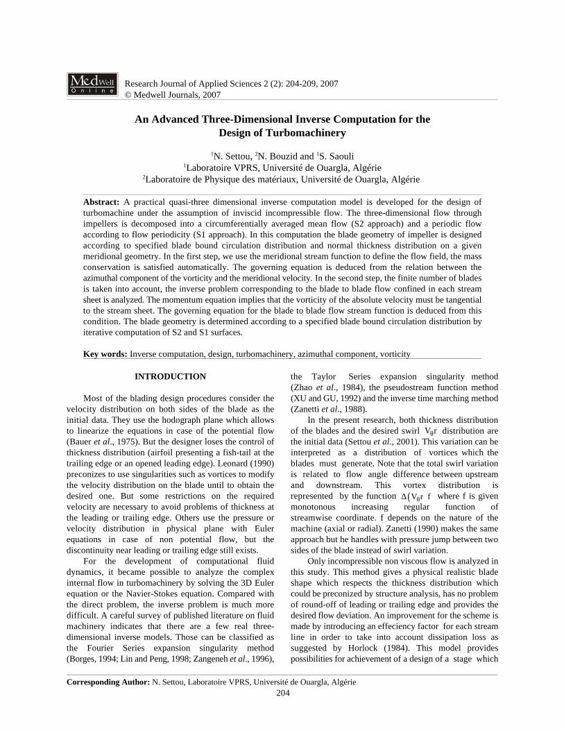
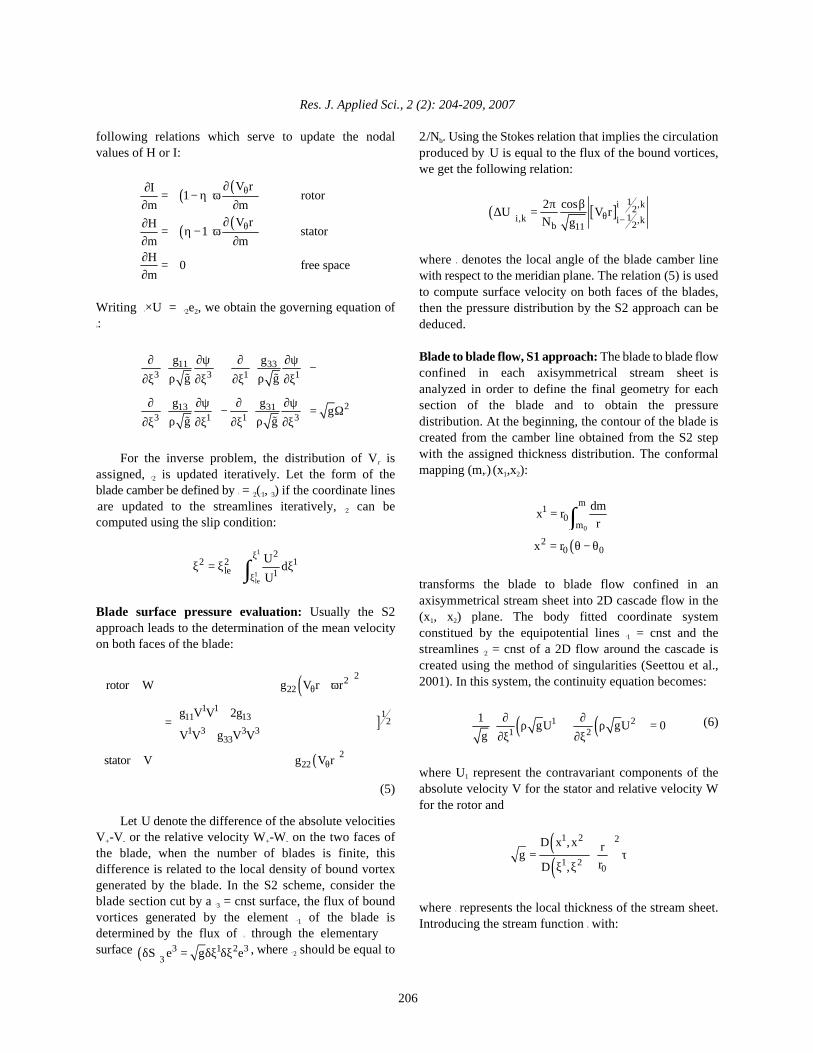
Fig. 1: Meridional plan of a multistage turbopump

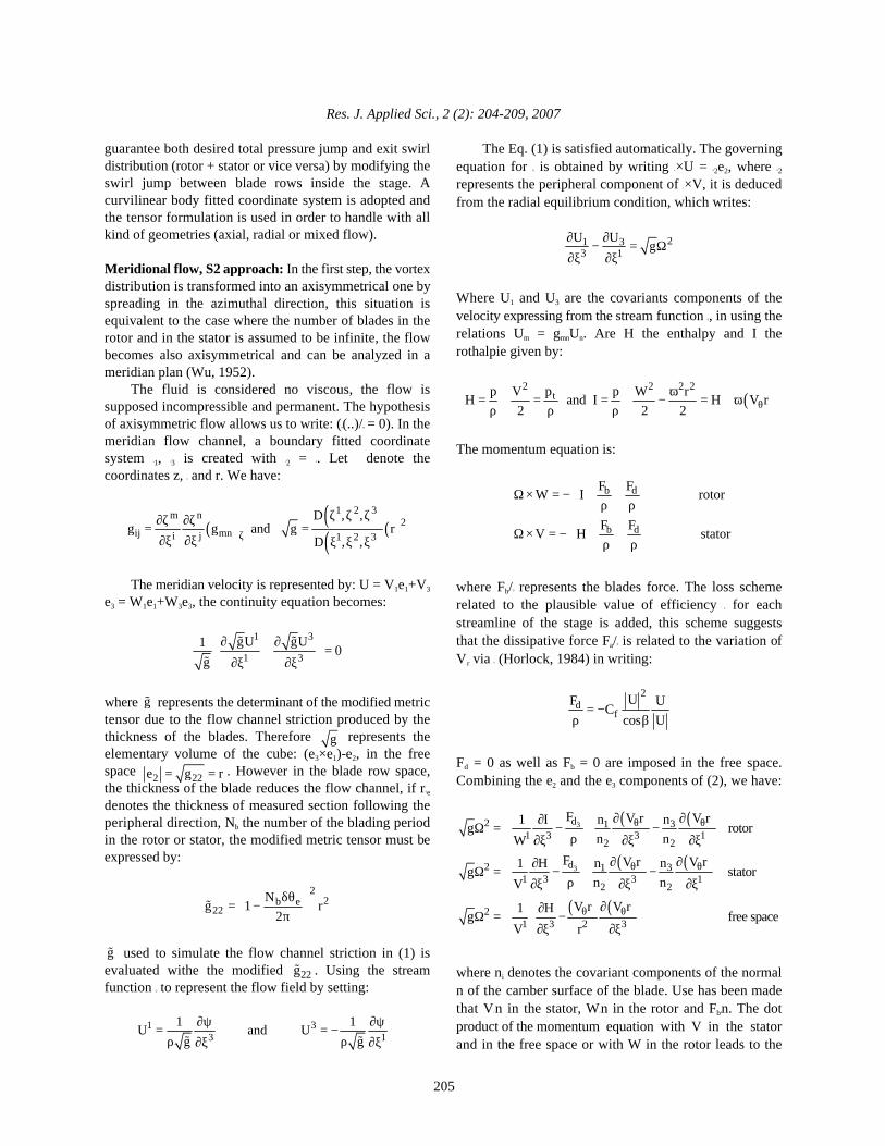
Fig. 2: Geometry of flow passage and computational mesh

The relation (6) is satisfied. From the momentumequation, we can show that the free vortex must betangential to the axisymmetrical stream sheet, thegoverning equation of the blade to blade flow streamfunction is deduced from this condition: for the relativeflow around the blades of the rotor, we have:

Boundary conditions for the inverse problem:

The solution of the inverse problem leads to thedetermination of flux penetration on the blade contour, thecamber line inclination correction * is given by:9

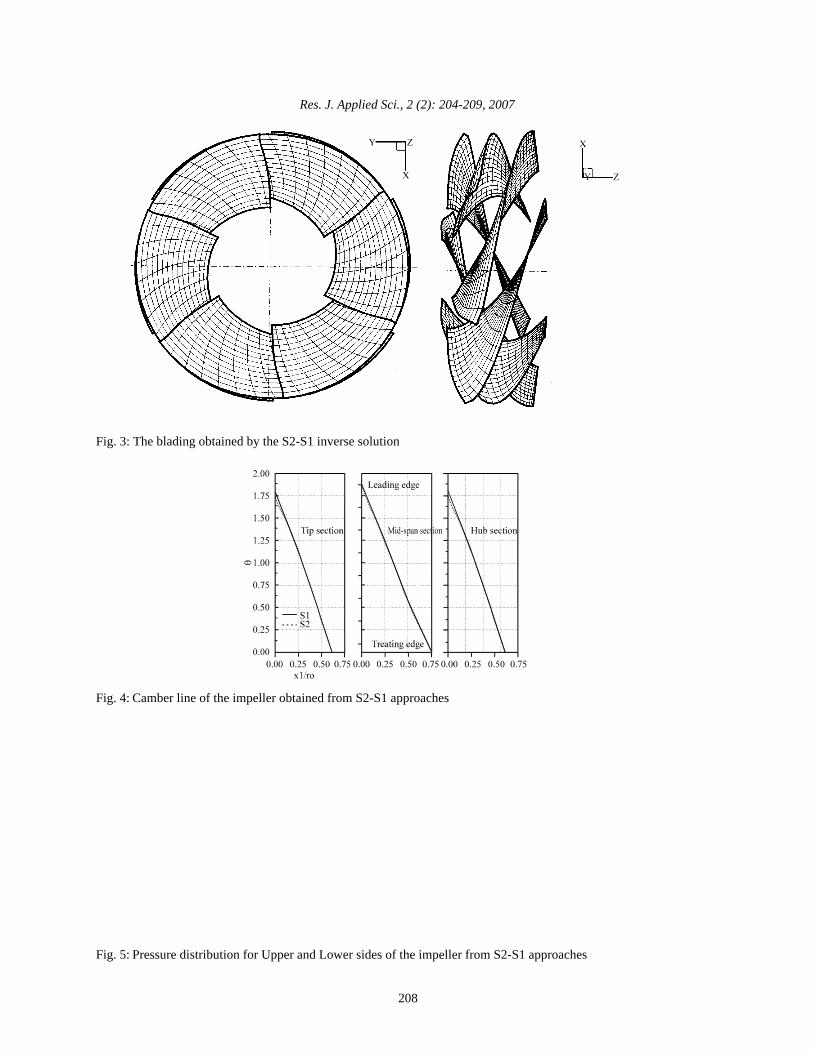
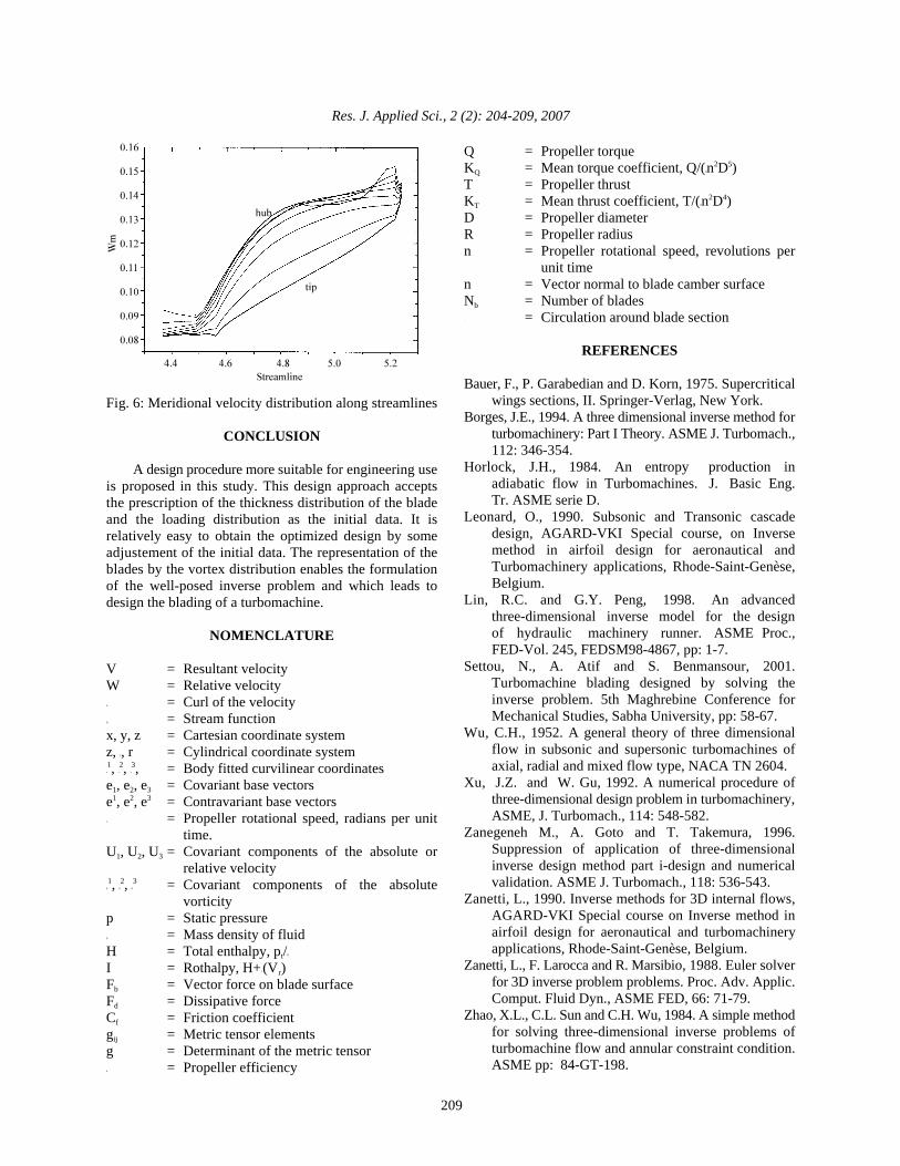
The design of a turbopump is presented in this study.Figure 1 shows the network in the meridional plan for themultistage turbopump. Figure 2 shows the network in themeridional plan obtained by the computation for the 2Dincompressible potential flow (Settou et al., 2001).Figure 3 shows the blading obtained by the S2-S1 inversesolution. Figure 4 shows the comparison of the camberlines of the impeller obtained from the S2 approach andrectified by the S1 approach. Figure 5 shows the pressuredistribution obtained from the S2-S1 calculation for theupper and the lower sides of blade. For the case of thecentrifugal impeller, the loading is optimised to avoid thecavitation. The results from the S2 and S1 computationsare similar, but not identical, the need of the S1computation to obtain the final geometry definition ofthe blades is confirmed. The meridional velocitydistributions along averaged mean flow streamlines areshown in Fig. 6.

Res. J. Applied Sci., 2 (2): 204-209, 2007

208

Fig. 3: The blading obtained by the S2-S1 inverse solution

Fig. 4: Camber line of the impeller obtained from S2-S1 approaches

Fig. 5: Pressure distribution for Upper and Lower sides of the impeller from S2-S1 approaches

Res. J. Applied Sci., 2 (2): 204-209, 2007

209

Fig. 6: Meridional velocity distribution along streamlines

CONCLUSION

A design procedure more suitable for engineering useis proposed in this study. This design approach acceptsthe prescription of the thickness distribution of the bladeand the loading distribution as the initial data. It isrelatively easy to obtain the optimized design by someadjustement of the initial data. The representation of theblades by the vortex distribution enables the formulationof the well-posed inverse problem and which leads todesign the blading of a turbomachine.

NOMENCLATURE

V = Resultant velocityW = Relative velocityS = Curl of the velocityQ = Stream functionx, y, z = Cartesian coordinate systemz, 2, r = Cylindrical coordinate system> , > , > , = Body fitted curvilinear coordinates1 2 3

e , e , e = Covariant base vectors1 2 3

e , e , e = Contravariant base vectors1 2 3

T = Propeller rotational speed, radians per unittime.

U , U , U = Covariant components of the absolute or1 2 3

relative velocityS , S , S = Covariant components of the absolute1 2 3

vorticityp = Static pressureD = Mass density of fluidH = Total enthalpy, p /Dt

I = Rothalpy, H+T(V )2r

F = Vector force on blade surfaceb

F = Dissipative forced

C = Friction coefficientf

g = Metric tensor elementsij

g = Determinant of the metric tensor0 = Propeller efficiency

Q = Propeller torqueK = Mean torque coefficient, Q/(Dn D )Q

2 5

T = Propeller thrustK = Mean thrust coefficient, T/(Dn D )T

2 4

D = Propeller diameterR = Propeller radiusn = Propeller rotational speed, revolutions per

unit timen = Vector normal to blade camber surfaceN = Number of bladesb

' = Circulation around blade section

REFERENCES

Bauer, F., P. Garabedian and D. Korn, 1975. Supercriticalwings sections, II. Springer-Verlag, New York.

Borges, J.E., 1994. A three dimensional inverse method forturbomachinery: Part I Theory. ASME J. Turbomach.,112: 346-354.

Horlock, J.H., 1984. An entropy production inadiabatic flow in Turbomachines. J. Basic Eng.Tr. ASME serie D.

Leonard, O., 1990. Subsonic and Transonic cascadedesign, AGARD-VKI Special course, on Inversemethod in airfoil design for aeronautical andTurbomachinery applications, Rhode-Saint-Genèse,Belgium.

Lin, R.C. and G.Y. Peng, 1998. An advancedthree-dimensional inverse model for the designof hydraulic machinery runner. ASME Proc.,FED-Vol. 245, FEDSM98-4867, pp: 1-7.

Settou, N., A. Atif and S. Benmansour, 2001.Turbomachine blading designed by solving theinverse problem. 5th Maghrebine Conference forMechanical Studies, Sabha University, pp: 58-67.

Wu, C.H., 1952. A general theory of three dimensionalflow in subsonic and supersonic turbomachines ofaxial, radial and mixed flow type, NACA TN 2604.

Xu, J.Z. and W. Gu, 1992. A numerical procedure ofthree-dimensional design problem in turbomachinery,ASME, J. Turbomach., 114: 548-582.

Zanegeneh M., A. Goto and T. Takemura, 1996.Suppression of application of three-dimensionalinverse design method part i-design and numericalvalidation. ASME J. Turbomach., 118: 536-543.

Zanetti, L., 1990. Inverse methods for 3D internal flows,AGARD-VKI Special course on Inverse method inairfoil design for aeronautical and turbomachineryapplications, Rhode-Saint-Genèse, Belgium.

Zanetti, L., F. Larocca and R. Marsibio, 1988. Euler solverfor 3D inverse problem problems. Proc. Adv. Applic.Comput. Fluid Dyn., ASME FED, 66: 71-79.

Zhao, X.L., C.L. Sun and C.H. Wu, 1984. A simple methodfor solving three-dimensional inverse problems ofturbomachine flow and annular constraint condition.ASME pp: 84-GT-198.