Embed Size (px)
Citation preview

Dublin Institute of TechnologyARROW@DIT
Doctoral Engineering
2013-11-01
An Adaptive Packet Aggregation Algorithm(AAM) for Wireless NetworksJianhua Deng [Thesis]DIT, [email protected]
Follow this and additional works at: http://arrow.dit.ie/engdocPart of the Digital Communications and Networking Commons
This Theses, Ph.D is brought to you for free and open access by theEngineering at ARROW@DIT. It has been accepted for inclusion inDoctoral by an authorized administrator of ARROW@DIT. For moreinformation, please contact [email protected], [email protected].
This work is licensed under a Creative Commons Attribution-Noncommercial-Share Alike 3.0 License
Recommended CitationDeng, J. : An Adaptive Packet Aggregation Algorithm (AAM) for Wireless Networks, Doctoral Thesis. Dublin Institute of Technology,2013.
Dublin Institute of TechnologyARROW@DIT
Articles Communications Network Research Institute
2014-02-12
An Adaptive Packet Aggregation Algorithm(AAM) for Wireless NetworksJianhua Deng
Follow this and additional works at: http://arrow.dit.ie/commartPart of the Digital Communications and Networking Commons
This Theses, Ph.D is brought to you for free and open access by theCommunications Network Research Institute at ARROW@DIT. It hasbeen accepted for inclusion in Articles by an authorized administrator ofARROW@DIT. For more information, please [email protected], [email protected].

An Adaptive Packet Aggregation
Algorithm (AAM) for Wireless Networks
by
Jianhua Deng
A thesis submitted to the Dublin Institute of Technology
for the degree of Doctor of Philosophy
Supervisor: Dr. Mark Davis
School of Electronic and Communications Engineering
November 2013

I
Acknowledgements
This thesis would not exist without the support from my supervisor, families and friends
etc. I am very happy to take this opportunity to give my appreciation to those people
who have helped and guided me during my graduate career.
First and foremost I would like to acknowledge my supervisor Dr. Mark Davis who
gave me the opportunity to study at the Communications Network Research Institute
(CNRI) in Dublin Institute of Technology (DIT) for several years and guided me on
how to do PhD research. Dr. Mark Davis has been tremendous supervisor proving me
invaluable guidance and advices about research, academic skills and the Ireland culture.
He is open-minded, supportive and caring. He gave me the confidence and knowledge
to help me to turn my dreams into reality. I own him a great many heartfelt thanks.
I also would like to express my gratitude to Prof. Gerald Farrell, Prof. Zhiguang Qin,
and Prof. Bing Wu, who helped me to gain the scholarship from China Scholarship
Council (CSC) and the opportunity of studying in DIT. Prof. Gerald Farrell gave me a
warm reception on the first day I arrived in DIT and I appreciate that he always is ready
to help me. Prof. Zhiguang Qin always gives me good suggestions and encourages me
to make plan for the future. Prof. Bing Wu leads me to know Ireland and introduced me
to Prof. Gerald Farrell. Prof. Bing Wu is very kind heart and friendly. I appreciate what
they have done for me.
During the life time in Ireland, the friendship always supports me. I apology I am not
listing you all by name and there is a few people mentioned: Dr. Mirosław Narbutt, Dr.
Tanmoy Debnath, Dr. Mustafa Ramadhan, Dr. Brian Keegan, Chengzhe Zhang, Yin
Chen, Dr. Rong Hu, Dr. Erqiang Zhou, Dr. Yi(熠) Ding, Jianfeng Wu, Fuhu Deng, Yi
(一) Ding, Dr. Yupeng Liu, Dr. Qiaohuan Chen, Bilu, Jenny, Panpan Lin, Albuto Dotto

II
and Claude Dyer. I have sweet memories from these friends of Dr. Rong Hu, Dr.
Erqiang Zhou, Dr. Yi (熠) Ding, Jianfeng Wu, Fuhu Deng, Yi (一) Ding who cooked for
me, discussed with me and made the house feel like home.
I would like to give high respect to my fantastic wife Rong Yang who always loves,
encourages and supports me since we met in seven years ago. Without her loves,
supports and sacrifices, this work would have never come to fruition. I would like to
thank Rong Yang for sharing these years and for brightening my life. In the middle of
the night of 14th
March 2011, the most original creation I was involved finally arrived,
Kaihao Deng, my dearest son. He makes my life different on every day from his birth.
He always uses his smiles and voices including laugh and cry to tell me that he loves
me which makes me powerful to face all of the difficulties.

III
Declaration
I certify that this thesis which I now submit for examination for the award of Doctor of
Philosophy, is entirely my own work and has not been taken from the work of others,
save and to the extent that such work has been cited and acknowledged within the text
of my work.
This thesis was prepared according to the regulations for postgraduate study by research
of the Dublin Institute of Technology (DIT) and has not been submitted in whole or in
part for another award in any other third level institution.
The work reported on in this thesis conforms to the principles and requirements of the
DIT's guidelines for ethics in research.
DIT has permission to keep, lend or copy this thesis in whole or in part, on condition
that any such use of the material of the thesis is duly acknowledged.
Signature __________________________________ Date ______________

IV
Abstract
Packet aggregation algorithms are used to improve the throughput performance by
combining a number of packets into a single transmission unit in order to reduce the
overhead associated with each transmission within a packet-based communications
network. However, the throughput improvement is also accompanied by a delay
increase. The biggest drawback of a significant number of the proposed packet
aggregation algorithms is that they tend to only optimize a single metric, i.e. either to
maximize throughput or to minimize delay. They do not permit an optimal trade-off
between maximizing throughput and minimizing delay. Therefore, these algorithms
cannot achieve the optimal network performance for mixed traffic loads containing a
number of different types of applications which may have very different network
performance requirements. In this thesis an adaptive packet aggregation algorithm
called the Adaptive Aggregation Mechanism (AAM) is proposed which achieves an
aggregation trade-off in terms of realizing the largest average throughput with the
smallest average delay compared to a number of other popular aggregation algorithms
under saturation conditions in wireless networks. The AAM algorithm is the first packet
aggregation algorithm that employs an adaptive selection window mechanism where the
selection window size is adaptively adjusted in order to respond to the varying nature of
both the packet size and packet rate. This algorithm is essentially a feedback control
system incorporating a hybrid selection strategy for selecting the packets. Simulation
results demonstrate that the proposed algorithm can (a) achieve a large number of sub-
packets per aggregate packet for a given delay and (b) significantly improve the
performance in terms of the aggregation trade-off for different traffic loads.
Furthermore, the AAM algorithm is a robust algorithm as it can significantly improve
the performance in terms of the average throughput in error-prone wireless networks.
V
Contents
Acknowledgements ............................................................................................................................................ I
Declaration ........................................................................................................................................................... III
Abstract .................................................................................................................................................................. IV
List of Figures .................................................................................................................................................. VIII
List of Tables .................................................................................................................................................... XIV
Abbreviations and Acronyms ................................................................................................................ XVII
Chapter 1 Introduction .................................................................................................................................... 1
1.1 Problem Statement ....................................................................................................................................... 2
1.2 Objectives and Contributions ................................................................................................................... 2
1.3 Organization..................................................................................................................................................... 4
Chapter 2 Technical Background .............................................................................................................. 6
2.1 IEEE 802.11 Wireless Local Area Networks ....................................................................................... 6
2.1.1 IEEE 802.11a standard ............................................................................................8 2.1.2 IEEE 802.11n Standard ...........................................................................................9 2.1.3 IEEE 802.11ac standard ....................................................................................... 10 2.1.4 Architecture of WLANs ........................................................................................ 10
2.2 IEEE 802.11 MAC Mechanism ................................................................................................................ 11
2.3 IEEE 802.11 Frames .................................................................................................................................. 15
2.3.1 IEEE 802.11 Data Frame Format ......................................................................... 15 2.3.2 IEEE 802.11 Control Frame Format .................................................................... 17 ACK Frame ....................................................................................................................... 17 2.3.3 IEEE 802.11 Management Frame Format .......................................................... 18
2.4 Transmission Errors in WLANs ............................................................................................................ 18
2.5 PHY Rate Adaption Mechanisms in WLANs ..................................................................................... 19
2.6 Network Simulators ................................................................................................................................... 21
2.7 Packet Sniffers .............................................................................................................................................. 25
2.8 Chapter Summary ....................................................................................................................................... 27
Chapter 3 Review of Packet Aggregation Algorithms ................................................................. 29
3.1 Throughput and Delay .............................................................................................................................. 29
3.1.1 Throughput ........................................................................................................... 29 3.1.2 Delay ...................................................................................................................... 32 3.1.3 Discussion of Throughput and Delay .................................................................. 33
3.2 Trade-off between Throughput and Delay ....................................................................................... 33
3.2.1 Delay Associated with a Packet Aggregation ..................................................... 34

VI
3.2.2 Trade-Off between Throughput and Delay ........................................................ 37 3.2.3 Discussion of Trade-off between Throughput and Delay .................................. 39
3.3 Packet Aggregation Algorithms ............................................................................................................ 40
3.3.1 Fixed with FIFO Packet Aggregation Algorithms (FF) ....................................... 42 3.3.2 Fixed with Non-FIFO Packet Aggregation Algorithms (FNF) ............................ 45 3.3.3 Adaptive with FIFO Packet Aggregation Algorithms (AF) ................................ 46 3.3.4 Adaptive with Non-FIFO Packet Aggregation Algorithms (ANF) ..................... 48 3.3.5 Transmission Errors and Packet Aggregation Algorithms................................ 50 3.3.6 Discussion of Packet Aggregation Algorithms ................................................... 50
3.4 A-MSDU and A-MPDU Schemes ............................................................................................................ 53
3.4.1 Discussion of A-MSDU and A-MPDU Schemes.................................................... 58 3.5 Chapter Summary ....................................................................................................................................... 59
Chapter 4 Proposed Packet Aggregation Algorithm .................................................................... 60
4.1 Adjustable Aggregation Algorithm (A3) ............................................................................................. 61
4.2 Aggregate Packet Analyzer (APA) ........................................................................................................ 66
4.3 Aggregate Tuning Algorithm (ATA) .................................................................................................... 67
4.4 User Specified Input Parameters .......................................................................................................... 69
4.5 Analysis of All Three Aggregation Algorithms ................................................................................ 70
4.6 Simulation ...................................................................................................................................................... 77
4.6.1 The Aggregation Process Only Scenario ............................................................. 79 4.6.2 Deployment Scenario in Wireless Networks ...................................................... 84
4.7 Chapter Summary ....................................................................................................................................... 89
Chapter 5 Results and Analysis ................................................................................................................ 91
5.1 Performance in the Scenario of Aggregation Process Only ....................................................... 91
5.1.1 Impact of the Selection Window Size on Performance ...................................... 92 5.1.2 CCDF of the Number of Sub-packets ................................................................... 95 5.1.3 CDF of the Sub-packet Delay ................................................................................ 98 5.1.4 Number of Sub-packets against Average Packet Delay ................................... 100 5.1.5 Conclusion ........................................................................................................... 102
5.2 Performance in Wireless Networks .................................................................................................. 103
5.2.1 Performance in an Ideal Wireless Network ..................................................... 104 Conclusion ..................................................................................................................... 114 5.2.2 Performance in an Error-Prone Wireless Network ......................................... 116 Conclusion ..................................................................................................................... 120
5.3 Chapter Summary ..................................................................................................................................... 121
Chapter 6 Conclusions and Future Work ......................................................................................... 124
6.1 Summary of Contributions and Achievements ............................................................................. 126
6.2 Open Problems and Future Work ...................................................................................................... 128
6.3 Publications ................................................................................................................................................. 134
VII
References ......................................................................................................................................................... 135
Appendix A ........................................................................................................................................................ 156
Appendix B ........................................................................................................................................................ 172
Appendix C ........................................................................................................................................................ 188
Appendix D ........................................................................................................................................................ 204

VIII
List of Figures
Figure 2-1: The use of Inter-Frame Spaces in accessing the medium …………………………12
Figure 2-2: An example of the DCF operation used to access the medium ……………………15
Figure 2-3: The generic IEEE 802.11 MAC data frame format ……………………..………………16
Figure 2-4: The Frame Control field in the IEEE 802.11 control frame…..................................17
Figure 2-5: The format of the IEEE 802.11 ACK frame…………………………………………………18
Figure 2-6: The format of the IEEE 802.11 management frame ……………………………18
Figure 2-7: calculating the new IEEE 802.11n PHY rate…………………………………………………19
Figure 2-8: The software organization of the ns-3 simulator……………………………23
Figure 2-9: Basic simulation of packet aggregation in ns-3 …………………………………25
Figure 2-10: The operation of a packet sniffer application in a wireless network environment...........................................................................................................................................................26
Figure 2-11: An Example of Wireshark captures packets and parses their contents ………27
Figure 3-1: The throughput against data rate without packet aggregation ………………31
Figure 3-2: An example of trade-off between throughput and delay for different aggregation algorithms ……………………………………………………………………………………………38
Figure 3-3: The aggregation process for packet aggregation algorithm in wireless networks ……………………………………………………………………………………………………………………41
Figure 3-4: The format of concatenation and packing ………………..…………………………… 43
Figure 3-5: The format of A-MSDU frame……………………………………………….…………………54
Figure 3-6: The format of A-MPDU frame……………………………………………………………………54
Figure 3-7: The relationship between A-MSDU and A-MPDU frames…………..………………….55
Figure 4-1: The structure of the AAM algorithm ………………………………………...…………………61
Figure 4-2: How packets are selected from the input buffer and moved into the output buffer ……………………………………………………………………………………………………………………….62
Figure 4-3: The flowchart of the A3 ….………………………………………………………….……………….63
Figure 4-4: The flowchart of the FIFO …………………………………………………………72
Figure 4-5: The flowchart of the SSFS ..…………………………………………………………………………73
Figure 4-6: The interaction between the different parameters of the FIFO algorithm……..74
Figure 4-7: The interaction between the different parameters of the SSFS algorithm……..75
Figure 4-8: The interaction between the different parameters of the AAM algorithm……..75
Figure 4-9: Flowchart showing the operation of the AAM algorithm………………………………81
IX
Figure 4-10: Flowchart showing the operation of the APA and ATA algorithms ……….……82
Figure 4-11: The topology of the wireless network in the ns-3 simulation …………………...84
Figure 4-12: The operation of the AAM algorithm in the ns-3 simulation….……………………85
Figure 5-1: The average packet rate for the captured traffic trace file 2 …………………………93
Figure 5-2: The selection window size of the one in ten aggregate packets generated for the captured traffic trace file 2 ……………………………………………………..……………………………94
Figure 5-3: The average packet rate for the captured traffic trace file 14 ……………………….94
Figure 5-4: The selection window size for the aggregate packets generated for all raw packets input for the captured traffic trace file 14 ………………………………………………………95
Figure 5-5: The CCDF of the number of sub-packets for the captured traffic trace file 2 …96
Figure 5-6: The CCDF of the number of sub-packets for the captured traffic trace file 14..97
Figure 5-7: The CDF of the sub-packet delay for the captured traffic trace file 2. …………99
Figure 5-8: The CDF of the sub-packet delay for the captured traffic trace file 14 ………99
Figure 5-9: The number of sub-packets against the average packet delay for the captured traffic trace file 2 ………………………………………………………………………………………………………101
Figure 5-10: The number of sub-packets against the average packet delay for the captured traffic trace file 14 ………………………………………………………………………………………………….....101
Figure 5-11: The throughput against data rate for the different PHY rates for the captured traffic trace file 2..……………………………………………………………………………………………………105
Figure 5-12: The throughput against data rate for the different PHY rates for the captured traffic trace file 14 ….................................................................................................................................106
Figure 5-13: The average delay against the data rate for the different PHY rates for the captured traffic trace file 2 ……………………………………………………………………………………108
Figure 5-14: The average delay against the data rate for the different PHY rates for the captured traffic trace file 14 ………………………………………………………………………………………109
Figure 5-15: The average aggregate packet size for the different PHY rates under saturation for the captured traffic trace file 2……………………………………………………………110
Figure 5-16: The average aggregate packet size for the different PHY rates under saturation for the captured traffic trace file 14. ………………………………………………………111
Figure 5-17: The mean square deviation for the different PHY rates under saturation for the captured traffic file 2.. …………………………………………………………………………………………112
Figure 5-18: The mean square deviation for the different PHY rates under saturation for the captured traffic file 14………………………………………………………………………………………112
Figure 5-19: The aggregation trade-off in terms of achieving the maximum average throughput with the minimum average delay for the capture traffic trace file 2……………113

X
Figure 5-20: The aggregation trade-off in terms of achieving the maximum average throughput with the minimum average delay for the capture traffic trace file 14. ……………………………………………………………………………………………………………………………113
Figure 5-21: The throughput against data rate for different BERs for the captured trace file 2 ………………………………………………………………………………………………………………………………116
Figure 5-22: The throughput against data rate for different BER for the captured trace file 14 ……….…………...................................................................................................................................................117
Figure 5-23: The maximum throughput against BER with a fixed data rate 26 Mbps for the captured traffic trace file 2 ………………………………………………………..………………………………118
Figure 5-24: The maximum throughput against BER with a fixed data rate 26 Mbps for the captured traffic trace file 14 ………………………………………………………………………………………118
Figure 5-25: The average PHY rate against BER with a fixed data rate of 26 Mbps for the captured traffic trace file 2 ………………………………………………………………………………………119
Figure 5-26: The average PHY rate against BERs with a fixed data rate of 26 Mbps for the captured traffic trace file 14 ………………………………………………………………………………………120
Figure A-1: The average packet rate for the captured traffic trace file 1. ………………………156
Figure A-2: The selection window size generated by the AAM algorithm for the first 32,000 aggregate packets for the captured traffic trace file 1. …………………………………………………156
Figure A-3: The average packet rate for the captured traffic trace file 2. ………………………157
Figure A-4: The selection window size generated by the AAM algorithm for the first 32,000 aggregate packets for the captured traffic trace file 2. …………………………………………………157
Figure A-5: The average packet rate for the captured traffic trace file 3. ....……………………158
Figure A-6: The selection window size generated by the AAM algorithm for the first 32,000 aggregate packets for the captured traffic trace file 3. …………………………………………………158
Figure A-7: The average packet rate for the captured traffic trace file 4. ………………………159
Figure A-8: The selection window size generated by the AAM algorithm for the first 32,000 aggregate packets for the captured traffic trace file 4. …………………………………………………159
Figure A-9: The average packet rate for the captured traffic trace file 5. .. ……………………..160
Figure A-10: The selection window size generated by the AAM algorithm for the first 32,000 aggregate packets for the captured traffic trace file 5. ...... …………………………………160
Figure A-11: The average packet rate for the captured traffic trace file 6. .............................. 161
Figure A-12: The selection window size generated by the AAM algorithm for the captured traffic trace file 6. ............................................................................................................................................. 161
Figure A-13: The average packet rate for the captured traffic trace file 7. .............................. 162
Figure A-14: The selection window size generated by the AAM algorithm for the captured traffic trace file 7. ............................................................................................................................................. 162
Figure A-15: The average packet rate for the captured traffic trace file 8. .............................. 163
XI
Figure A-16: The selection window size generated by the AAM algorithm for the captured traffic trace file 8. ............................................................................................................................................. 163
Figure A-17: The average packet rate for the captured traffic trace file 9. .............................. 164
Figure A-18: The selection window size generated by the AAM algorithm for the captured traffic trace file 9. ............................................................................................................................................. 164
Figure A-19: The average packet rate for the captured traffic trace file 10. ........................... 165
Figure A-20: The selection window size generated by the AAM algorithm for the captured traffic trace file 10. ........................................................................................................................................... 165
Figure A-21: The average packet rate for the captured traffic trace file 11. ........................... 166
Figure A-22: The selection window size generated by the AAM algorithm for the captured traffic trace file 11. ........................................................................................................................................... 166
Figure A-23: The average packet rate for the captured traffic trace file 12. ........................... 167
Figure A-24: The selection window size generated by the AAM algorithm for the captured traffic trace file 12. ........................................................................................................................................... 167
Figure A-25: The average packet rate for the captured traffic trace file 13. ........................... 168
Figure A-26: The selection window size generated by the AAM algorithm for the captured traffic trace file 13. ........................................................................................................................................... 168
Figure A-27: The average packet rate for the captured traffic trace file 14. ........................... 169
Figure A-28: The selection window size generated by the AAM algorithm for the captured traffic trace file 14. ........................................................................................................................................... 169
Figure A-29: The average packet rate for the captured traffic trace file 15. ........................... 170
Figure A-30: The selection window size generated by the AAM algorithm for the captured traffic trace file 15. ........................................................................................................................................... 170
Figure A-31: The average packet rate for the captured traffic trace file 16. ........................... 171
Figure A-32: The selection window size generated by the AAM algorithm for the captured traffic trace file 16. ........................................................................................................................................... 171
Figure B-1: The CCDF of the number of sub-packets for the captured traffic trace file 1. . 172
Figure B-2: The CCDF of the number of sub-packets for the captured traffic trace file 2. . 173
Figure B-3: The CCDF of the number of sub-packets for the captured traffic trace file 3. . 174
Figure B-4: The CCDF of the number of sub-packets for the captured traffic trace file 4. . 175
Figure B-5: The CCDF of the number of sub-packets for the captured traffic trace file 5. . 176
Figure B-6: The CCDF of the number of sub-packets for the captured traffic trace file 6. . 177
Figure B-7: The CCDF of the number of sub-packets for the captured traffic trace file 7. . 178
Figure B-8: The CCDF of the number of sub-packets for the captured traffic trace file 8. . 179
Figure B-9: The CCDF of the number of sub-packets for the captured traffic trace file 9. . 180

XII
Figure B-10: The CCDF of the number of sub-packets for the captured traffic trace file 10. .................................................................................................................................................................................. 181
Figure B-11: The CCDF of the number of sub-packets for the captured traffic trace file 11. …………………………………………………………………………………………………………………………………182
Figure B-12: The CCDF of the number of sub-packets for the captured traffic trace file 12. ……………………………………………………………………………………………………………………………183
Figure B-13: The CCDF of the number of sub-packets for the captured traffic trace file 13. ……………………………………………………………………………………………………………………………184
Figure B-14: The CCDF of the number of sub-packets for the captured traffic trace file 14. ……………………………………………………………………………………………………………………………185
Figure B-15: The CCDF of the number of sub-packets for the captured traffic trace file 15. ……………………………………………………………………………………………………………………………186
Figure B-16: The CCDF of the number of sub-packets for the captured traffic trace file 16. ……………………………………………………………………………………………………………………………187
Figure C-1: The CDF of sub-packet delay for the captured traffic trace file 1. ........................ 188
Figure C-2: The CDF of sub-packet delay for the captured traffic trace file 2. ........................ 189
Figure C-3: The CDF of sub-packet delay for the captured traffic trace file 3. ........................ 190
Figure C-4: The CDF of sub-packet delay for the captured traffic trace file 4. ........................ 191
Figure C-5: The CDF of sub-packet delay for the captured traffic trace file 5. ........................ 192
Figure C-6: The CDF of sub-packet delay for the captured traffic trace file 6. ........................ 193
Figure C-7: The CDF of sub-packet delay for the captured traffic trace file 7. ........................ 194
Figure C-8: The CDF of sub-packet delay for the captured traffic trace file 8. ........................ 195
Figure C-9: The CDF of sub-packet delay for the captured traffic trace file 9. ........................ 196
Figure C-10: The CDF of sub-packet delay for the captured traffic trace file 10. ................... 197
Figure C-11: The CDF of sub-packet delay for the captured traffic trace file 11. ................... 198
Figure C-12: The CDF of sub-packet delay for the captured traffic trace file 12. ................... 199
Figure C-13: The CDF of sub-packet delay for the captured traffic trace file 13. ................... 200
Figure C-14: The CDF of sub-packet delay for the captured traffic trace file 14. ................... 201
Figure C-15: The CDF of sub-packet delay for the captured traffic trace file 15. ................... 202
Figure C-16: The CDF of sub-packet delay for the captured traffic trace file 16. ................... 203
Figure D-1: The number of sub-packets against the average packet delay for the captured traffic trace file1................................................................................................................................................ 204
Figure D-2: The number of sub-packets against the average packet delay for the captured traffic trace file 2. ............................................................................................................................................. 205
XIII
Figure D-3: The number of sub-packets against the average packet delay for the captured traffic trace file 3. ............................................................................................................................................. 206
Figure D-4: The number of sub-packets against the average packet delay for the captured traffic trace file 4. ............................................................................................................................................. 207
Figure D-5: The number of sub-packets against the average packet delay for the captured traffic trace file 5. ............................................................................................................................................. 208
Figure D-6: The number of sub-packets against the average packet delay for the captured traffic trace file 6. ............................................................................................................................................. 209
Figure D-7: The number of sub-packets against the average packet delay for the captured traffic trace file 7. ............................................................................................................................................. 210
Figure D-8: The number of sub-packets against the average packet delay for the captured traffic trace file 8. ………………………………………………………………………………………………………211
Figure D-9: The number of sub-packets against the average packet delay for the captured traffic trace file 9. ............................................................................................................................................. 212
Figure D-10: The number of sub-packets against the average packet delay for the captured traffic trace file 10. ........................................................................................................................................... 213
Figure D-11: The number of sub-packets against the average packet delay for the captured traffic trace file 11. ........................................................................................................................................... 214
Figure D-12: The number of sub-packets against the average packet delay for the captured traffic trace file 12. ........................................................................................................................................... 215
Figure D-13: The number of sub-packets against the average packet delay for the captured traffic trace file 13. ........................................................................................................................................... 216
Figure D-14: The number of sub-packets against the average packet delay for the captured traffic trace file 14. ........................................................................................................................................... 217
Figure D-15: The number of sub-packets against the average packet delay for the captured traffic trace file 15. ........................................................................................................................................... 218
Figure D-16: The number of sub-packets against the average packet delay for the captured traffic trace file 16. ........................................................................................................................................... 219

XIV
List of Tables
Table 2-1: The IEEE 802.11 family of some WLAN standards …………………….……………………8
Table 2-2: The values of slot time, SIFS, DIFS and CW for different IEEE 802.11 standards……………………………………………………………………………………………………………………13
Table 2-3: The details of the data rate for IEEE standards 802.11b/g/n…………………………19
Table 3-1: The PHY parameter values for some of the IEEE 802.11 standards..………… 31
Table 3-2: A comparison between some packet aggregation algorithms ……………………..…52
Table 4-1: The rules of tuning the size N of the selection window ………………………..………68
Table 4-2: The details of 16 captured traffic trace files ……………………………………..…………78
Table 4-3: Explanation of the key parameters used in the C++ simulation ……………………79
Table 4-4: An example of the calculation of the aggregate packet delay …………………………80
Table 4-5: The definitions of the performance metrics for the AAM algorithm in the scenario of aggregation process only…..………………………………………………………………………83
Table 4-6: The list of the modified ns-3 module files …………………………….………………………86
Table 4-7: The simulation parameters used to implement the AAM algorithm in ns-3 ……87
Table 4-8: The performance metrics for analysis the AAM algorithm in the deployment scenario in wireless networks ….………………..………………………………………..……………………….88
Table 5-1: Some details of the captured traffic trace files 2 and 14 ………………………………91
Table 6-1: The rules for tuning the step size of selection window size…………………….……131
Table A-1: The details for the captured traffic trace file 1. ............................................................. 156
Table A-2: The details for the captured traffic trace file 2. ............................................................. 157
Table A-3: The details for the captured traffic trace file 3. ............................................................. 158
Table A-4: The details for the captured traffic trace file 4. ............................................................. 159
Table A-5: The details for the captured traffic trace file 5. ............................................................. 160
Table A-6: The details for the captured traffic trace file 6. ............................................................. 161
Table A-7: The details for the captured traffic trace file 7. ............................................................. 162
Table A-8: The details for the captured traffic trace file 8. ............................................................. 163
Table A-9: The details for the captured traffic trace file 9. ............................................................. 164
Table A-10: The details for the captured traffic trace file 10. ........................................................ 165
Table A-11: The details for the captured traffic trace file 11. ........................................................ 166
Table A-12: The details for the captured traffic trace file 12. ........................................................ 167
Table A-13: The details for the captured traffic trace file 13. ........................................................ 168
XV
Table A-14: The details for the captured traffic trace file 14. ........................................................ 169
Table A-15: The details for the captured traffic trace file 15. ........................................................ 170
Table A-16: The details for the captured traffic trace file 16. ........................................................ 171
Table B-1: The details for the captured traffic trace file 1 .............................................................. 172
Table B-2: The details for the captured traffic trace file 2. ............................................................. 173
Table B-3: The details for the captured traffic trace file 3. ............................................................. 174
Table B-4: The details for the captured traffic trace file 4. ............................................................. 175
Table B-5: The details for the captured traffic trace file 5. ............................................................. 176
Table B-6: The details for the captured traffic trace file 6. ............................................................. 177
Table B-7: The details for the captured traffic trace file 7 .............................................................. 178
Table B-8: The details for the captured traffic trace file 8. ............................................................. 179
Table B-9: The details for the captured traffic trace file 9. ............................................................. 180
Table B-10: The details for the captured traffic trace file 10. ........................................................ 181
Table B-11: The details for the captured traffic trace file 11. ........................................................ 182
Table B-12: The details for the captured traffic trace file 12. ........................................................ 183
Table B-13: The details for the captured traffic trace file 13. ........................................................ 184
Table B-14: The details for the captured traffic trace file 14. ........................................................ 185
Table B-15: The details for the captured traffic trace file 15. ........................................................ 186
Table B-16: The details for the captured traffic trace file 16. ........................................................ 187
Table C-1: The details for the captured traffic trace file 1. ............................................................. 188
Table C-2: The details for the captured traffic trace file 2. ............................................................. 189
Table C-3: The details for the captured traffic trace file 3. ............................................................. 190
Table C-4: The details for the captured traffic trace file 4. ............................................................. 191
Table C-5: The details for the captured traffic trace file 5. ............................................................. 192
Table C-6: The details for the captured traffic trace file 6. ............................................................. 193
Table C-7: The details for the captured traffic trace file 7. ............................................................. 194
Table C-8: The details for the captured traffic trace file 8. ............................................................. 195
Table C-9: The details for the captured traffic trace file 9 .............................................................. 196
Table C-10: The details for the captured traffic trace file 10. ........................................................ 197
Table C-11: The details for the captured traffic trace file 11 ......................................................... 198
Table C-12: The details for the captured traffic trace file 12. ........................................................ 199

XVI
Table C-13: The details for the captured traffic trace file 13. ........................................................ 200
Table C-14: The details for the captured traffic trace file 14. ........................................................ 201
Table C-15: The details for the captured traffic trace file 15. ........................................................ 202
Table C-16: The details for the captured traffic trace file 16. ........................................................ 203
Table D-1: The details for the captured traffic trace file 1. ............................................................. 204
Table D-2: The details for the captured traffic trace file 2. ............................................................. 205
Table D-3: The details for the captured traffic trace file 3. ............................................................. 206
Table D-4: The details for the captured traffic trace file 4. ............................................................. 207
Table D-5: The details for the captured traffic trace file 5. ............................................................. 208
Table D-6: The details for the captured traffic trace file 6. ............................................................. 209
Table D-7: The details for the captured traffic trace file 7. ............................................................. 210
Table D-8: The details for the captured traffic trace file 8. ............................................................. 211
Table D-9: The details for the captured traffic trace file 9. ............................................................. 212
Table D-10: The details for the captured traffic trace file 10. ........................................................ 213
Table D-11: The details for the captured traffic trace file 11. ........................................................ 214
Table D-12: The details for the captured traffic trace file 12. ........................................................ 215
Table D-13: The details for the captured traffic trace file 13. ........................................................ 216
Table D-14: The details for the captured traffic trace file 14. ........................................................ 217
Table D-15: The details for the captured traffic trace file 15. ........................................................ 218
Table D-16: The details for the captured traffic trace file 16. ........................................................ 219
XVII
Abbreviations and Acronyms
A3
Adjustable Aggregation Algorithm
AAM
Adaptive Aggregation Mechanism
AARF
Adaptive auto rate fallback
ACK
Acknowledgement
AD
Additive Decrease
AF
Adaptive with FIFO Packet Aggregation Algorithms
AI
Additive Increase
AIMD
Additive Increase Multiplicative Decrease
A-MPDU Aggregate MAC Protocol Data Unit
A-MSDU Aggregate MAC Service Data Unit
ANF
Adaptive with Non-FIFO Packet Aggregation Algorithms
AP
Access Point
APA
Aggregate Packet Analyzer
API
Application Program Interface
ARF
Auto Rate Fallback
ATA
Aggregate Tuning Algorithm
BA
Block ACK
BC
Back-off Counter
BER
Bit Error Rate
BSS
Basic Service Set
CCDF
Complementary Cumulative Distribution Function
CDF
Cumulative Distribution Function
CRC
Cyclic Redundancy Check
CSMA/CA Carrier Sense Multiple Access with Collision Avoidance
CTS
Clear-to-Send
CW
Contention Window
DCF
Distribution Coordination Function
DIFS
DCF Inter Frame Space
XVIII
DLL
Delay Lower Limit
DDSS
Direct Sequence Spread Spectrum
DTMC
Discrete Time Markov Chain
EIFS
Extended Inter-Frame Space
FCS
Frame Check Sequence
FER
Frame Error Rate
FF
Fixed with FIFO Packet Aggregation Algorithms
FHSS
Frequency Hopping Spread Spectrum
FIFO
First-In First-Out
FNF
Fixed with Non-FIFO Packet Aggregation Algorithms
FR
Frame Relay
FSE
Frame Size Estimation
Gbps
Gigabits Per Second
HCF
Hybrid Coordination Function
IBSS
Independent Basic Service Set
IEEE
Institute of Electrical and Electronics Engineers
IR
Infrared
ISM
Industrial, Scientific and Medical
LLC
Logical Link Control
MAC
Medium Access Control
Mbps
Megabits Per Second
MD
Multiplicative Decrease
MI
Multiplicative Increase
MIMO
Multiple-Input Multiple-Output
MU-MIMO Multi-user MIMO
NAV
Network Allocation Vector
NEST
Network Simulator Test-bed
OFDM
Orthogonal Frequency Division Multiplexing
Point Coordination Function
XIX
PHY
Physical Layer
PIFS
PCF Inter-Frame Space
PLCP
Physical Layer Convergence Protocol
PPDU
Physical Layer Protocol Unit
PS-Poll
Power-Saver Poll
QAM
Quadrature Amplitude Modulation
QoS
Quality of Service
RTS
Request-to-Send
SIFS
Short Inter-Frame Space
SSFS
Smallest-Size First-Served
TUL
Throughput Upper Limit
VoIP
Voice over IP
WDS
Wireless Distribution System
WLANs
Wireless local area networks
WMANs
Wireless Metropolitan Area Networks
WMNs
Wireless Mesh Networks
WNICs
Wireless Network Interface Controllers
WPANs
Wireless Personal Area Networks
WWANs
Wireless Wide Area Networks

1
Chapter 1 Introduction
In 1997 the IEEE LAN/MAN Standards Committee approved the first version of the
IEEE 802.11 standard [IEE97]. Since then, there have been numerous amendments to
the standard to achieve the goal of realizing ever higher throughputs. Increasing the
transmission rate and the use of ever more complex modulation schemes have allowed
for a further improvement in the throughput performance in wireless local area
networks (WLANs). However, as a consequence of the protocol headers, there exists an
upper limit on the achievable throughput which has been demonstrated by the authors in
[XiR02] where a lower limit on the delay has also been demonstrated. The existence of
such limits indicate that simply increasing the data rate without reducing the PHY
(Physical Layer) and MAC (Medium Access Control) overheads is bounded even if the
data rate is increased indefinitely. This has lead to the use of packet aggregation where
the throughput is increased as the protocol headers are reduced by combining a number
of small size packets into a single large size (or aggregate) packet.
Packet aggregation is the process of combining multiple packets together into a single
transmission unit in order to reduce the overhead associated with each transmission
within a packet-based communications network. In 2009 the IEEE 802.11n standard
defined two packet aggregation algorithms that are also employed in the IEEE 802.11ac
standard draft: Aggregate MAC Service Data Unit (A-MSDU) and Aggregate MAC
Protocol Data Unit (A-MPDU). However, the throughput improvement is also
associated with a delay increase as the packet aggregation algorithm may have to wait
for packets to arrive in order to be assembled into an aggregate packet.
2
1.1 Problem Statement
As most of the proposed packet aggregation algorithms don’t take account of the
varying nature of the traffic loads particularly the random nature of the packet size and
packet rate, these algorithms tend to optimize a single metric, i.e. either to maximize
throughput or to minimize delay. In general, they do not permit an optimal trade-off
between the two metrics which would allow for greater flexibility in operating under a
wide range of mixed traffic loads.
Generally, in modern networks the traffic load is a mix of different types of application
(e.g. VoIP and E-mail) which often have very different network performance
requirements. Consequently, optimal network performance cannot be achieved
simultaneously for mixed traffic loads by employing a packet aggregation algorithm
that only optimizes a single metric.
So there is a need for an adaptive packet aggregation algorithm that is better suited to
the mixed traffic loads found in modern data networks. This adaptive algorithm not only
achieves an optimal trade-off between maximizing throughput and minimizing delay in
a data network but also provides a good performance over a wide range of mixed traffic
loads.
1.2 Objectives and Contributions
In this thesis an adaptive packet aggregation algorithm called the Adaptive Aggregation
Mechanism (AAM) is proposed which can operate over a wide range of different traffic
loads in order to achieve the best aggregation trade-off in terms of realizing the largest
average throughput with the smallest average delay compared to a number of other
popular aggregation algorithms under saturation conditions in wireless networks. The
AAM algorithm is a robust adaptive packet aggregation algorithm where a feedback
control scheme incorporating a hybrid selection strategy and a tunable selection window
3
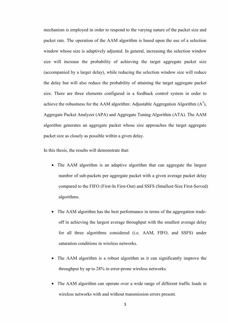
mechanism is employed in order to respond to the varying nature of the packet size and
packet rate. The operation of the AAM algorithm is based upon the use of a selection
window whose size is adaptively adjusted. In general, increasing the selection window
size will increase the probability of achieving the target aggregate packet size
(accompanied by a larger delay), while reducing the selection window size will reduce
the delay but will also reduce the probability of attaining the target aggregate packet
size. There are three elements configured in a feedback control system in order to
achieve the robustness for the AAM algorithm: Adjustable Aggregation Algorithm (A3),
Aggregate Packet Analyzer (APA) and Aggregate Tuning Algorithm (ATA). The AAM
algorithm generates an aggregate packet whose size approaches the target aggregate
packet size as closely as possible within a given delay.
In this thesis, the results will demonstrate that:
The AAM algorithm is an adaptive algorithm that can aggregate the largest
number of sub-packets per aggregate packet with a given average packet delay
compared to the FIFO (First-In First-Out) and SSFS (Smallest-Size First-Served)
algorithms.
The AAM algorithm has the best performance in terms of the aggregation trade-
off in achieving the largest average throughput with the smallest average delay
for all three algorithms considered (i.e. AAM, FIFO, and SSFS) under
saturation conditions in wireless networks.
The AAM algorithm is a robust algorithm as it can significantly improve the
throughput by up to 28% in error-prone wireless networks.
The AAM algorithm can operate over a wide range of different traffic loads in
wireless networks with and without transmission errors present.

4
1.3 Organization
This thesis is organized as follows.
Chapter 2 describes the main technologies that are used throughout the course of this
research by introducing the general technical background regarding wireless networks
before concentrating on the operation of packet aggregation. Chapter 2 overviews parts
of the IEEE 802.11 standards, the architecture of the WLANs, the MAC mechanism of
the IEEE 802.11 standards and the structure of the IEEE 802.11 frames which are
relevant to the thesis. The transmission errors in WLANs, the PHY rate adaption
mechanism, network simulator and packet sniffer are also discussed in the final sections
of this chapter.
Chapter 3 provides a literature review of packet aggregation algorithms in WLANs that
have been proposed by other researchers. This chapter also highlights the recent
advances in the area of packet aggregation research.
Chapter 4 describes the design and the development of the AAM algorithm. A
fundamental analysis of the AAM algorithm is presented after a detailed description of
each stage of the proposed algorithm. A description of the simulation process for the
AAM algorithm implemented in two different test scenarios is given that includes all
the modeling assumptions adopted in the simulation.
Chapter 5 presents the results for the two performance validation test scenarios. The
first section analyses the performance of the AAM algorithm aggregation process only.
The next section presents the results of the AAM algorithm when it is implemented in
wireless networks with and without transmission errors present. A comparison between
the performances is provided in order to further highlight the advantages of the AAM

5
algorithm compared to two other aggregation algorithms (i.e. FIFO and SSFS) based on
16 captured traffic trace files.
Chapter 6 provides a summary of the main findings and conclusions from this research
carried out. This chapter also gives some suggestions for the future research in this area.
6
Chapter 2 Technical Background
In this chapter, relevant background knowledge about IEEE 802.11 wireless local area
networks (WLANs), the IEEE 802.11 MAC mechanism, transmission errors and PHY
rate adaption mechanism in WLANs, network simulators and packet sniffers will be
introduced. In the first section, an introduction to the main standards of IEEE 802.11
WLANs and the architecture of wireless networks are presented. The second section
focuses on the MAC mechanism of the IEEE 802.11 WLAN standards and then the
formats of some of the IEEE 802.11 frames are presented. The detrimental impact of
transmission errors in WLANs are described in the fourth section and some PHY rate
adaption mechanisms are introduced in the following section. A discussion of the
network simulator ns-3 is given in the sixth section and the packet sniffer application
Wireshark is described in the last section.
2.1 IEEE 802.11 Wireless Local Area Networks
In the last decade, Wireless Local Area Networks (WLANs) based on the IEEE 802.11
standards have been widely employed in the home and enterprise networks across the
world. The IEEE 802.11 standard was approved by the IEEE LAN/MAN Standards
Committee in 1997 [IEE97]. The original version of the IEEE 802.11 standard defined a
single Medium Access Control (MAC) accessed by the Carrier Sense Multiple Access
with Collision Avoidance (CSMA/CA) mechanism and a Physical Layer (PHY) which
defined PHY rates of 1 Mbps and 2 Mbps. The PHY defined three types of modulation
technique: Infrared (IR), Frequency Hopping Spread Spectrum (FHSS) and Direct
Sequence Spread Spectrum (DSSS).
Further enhancements to the original standard, namely the IEEE 802.11b [IEEb99] and
IEEE 802.11a [IEa99] standards were both published in 1999. The IEEE 802.11b
7
standard supports 1, 2, 5.5 and 11 Mbps PHY rates in the license-free 2.4 GHz ISM
(Industrial, Scientific and Medical) band, while the IEEE 802.11a standard by using the
Orthogonal Frequency Division Multiplexing (OFDM) provides 8 PHY rates (i.e. 6, 9,
12, 18, 24, 36, 48 Mbps and 54 Mbps) in the license-free 5 GHz ISM band. In June of
2003, the IEEE 802.11g [IEE03] standard was approved which provides a maximum 54
Mbps PHY rate in the 2.4 GHz ISM band. The IEEE 802.11n standard [IEn09] was
published in September of 2009 which allows for a maximum of 100 Mbps PHY rate in
both the 2.4 GHz and 5 GHz ISM bands by using channel bonding with up to 72 Mbps
without channel bonding. The new multiple antenna technology MIMO (Multiple-Input
Multiple-Output) and the packet aggregation are employed in the IEEE 802.11n
standard. The standard for the next generation of wireless networks is the IEEE
802.11ac which is still under development. The draft 5.0 was published at the beginning
of 2013 [IEE13]. It provides higher throughput for WLANs on the 5 GHz ISM bands
[R&S11]. Theoretically, this specification will enable multi-station WLAN throughput
of at least 1 Gbps and a maximum single link throughput of at least 500 Mbps by using
some new technologies, such as extended channel bonding, Multi-user MIMO (MU-
MIMO) and packet aggregation [Any12]. The IEEE 802.11ac will provide backwards
compatibility with the IEEE 802.11a and IEEE 802.11n devices operating in the 5 GHz
ISM band [War12]. The IEEE 802.11ac standard is expected to be ratified in the early
2014 and the maximum PHY rate will be in excess of 5 Gbps.
Some members of the IEEE 802.11 family of standards are shown in Table 2-1 where
there are 5 main versions: IEEE 802.11a, IEEE 802.11b, IEEE 802.11g, IEEE 802.11n
which are now widely used to provide wireless connectivity in homes and businesses,
and the latest standard IEEE 802.11 ac is still under development.
8
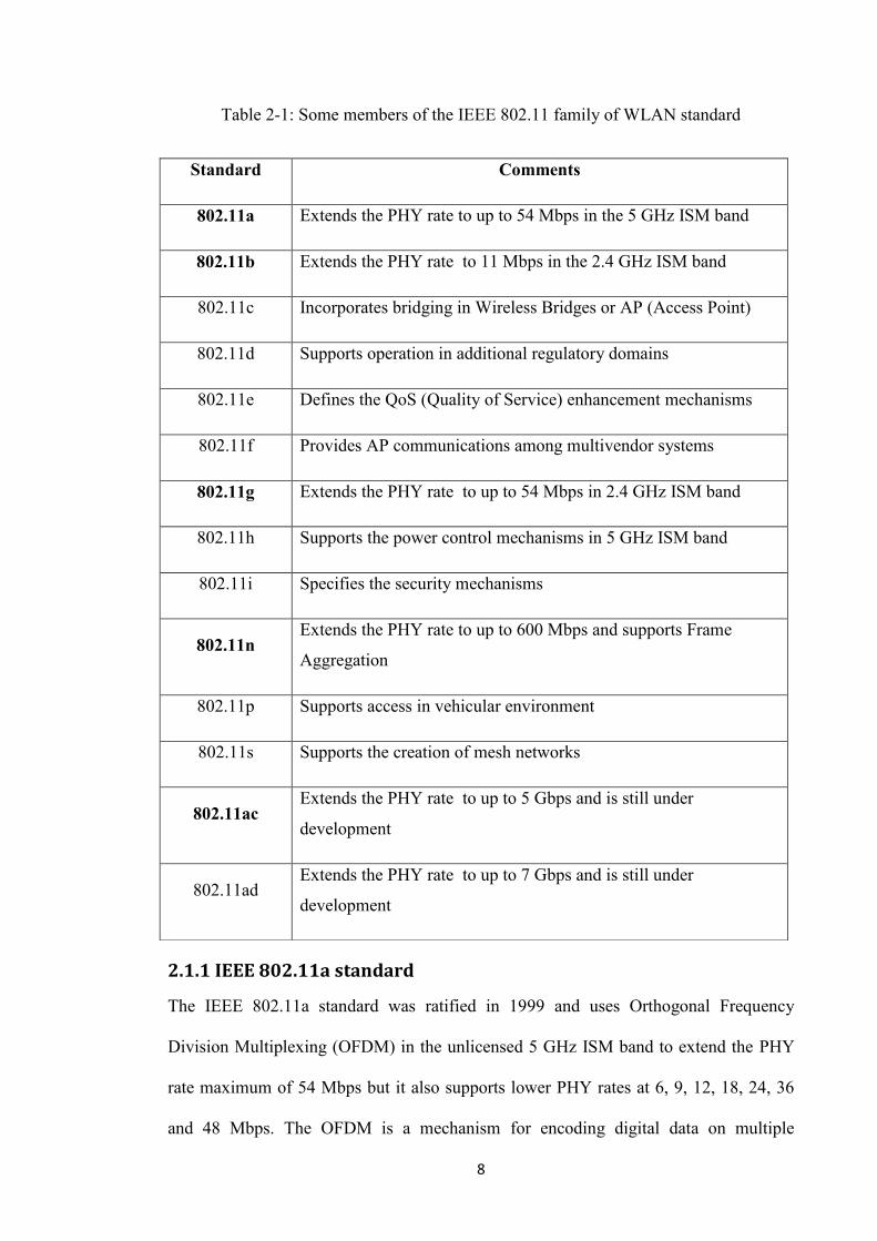
Table 2-1: Some members of the IEEE 802.11 family of WLAN standard
2.1.1 IEEE 802.11a standard
The IEEE 802.11a standard was ratified in 1999 and uses Orthogonal Frequency
Division Multiplexing (OFDM) in the unlicensed 5 GHz ISM band to extend the PHY
rate maximum of 54 Mbps but it also supports lower PHY rates at 6, 9, 12, 18, 24, 36
and 48 Mbps. The OFDM is a mechanism for encoding digital data on multiple
Standard Comments
802.11a Extends the PHY rate to up to 54 Mbps in the 5 GHz ISM band
802.11b Extends the PHY rate to 11 Mbps in the 2.4 GHz ISM band
802.11c Incorporates bridging in Wireless Bridges or AP (Access Point)
802.11d Supports operation in additional regulatory domains
802.11e Defines the QoS (Quality of Service) enhancement mechanisms
802.11f Provides AP communications among multivendor systems
802.11g Extends the PHY rate to up to 54 Mbps in 2.4 GHz ISM band
802.11h Supports the power control mechanisms in 5 GHz ISM band
802.11i Specifies the security mechanisms
802.11n Extends the PHY rate to up to 600 Mbps and supports Frame
Aggregation
802.11p Supports access in vehicular environment
802.11s Supports the creation of mesh networks
802.11ac Extends the PHY rate to up to 5 Gbps and is still under
development
802.11ad Extends the PHY rate to up to 7 Gbps and is still under
development

9
orthogonal subcarriers [IEa99]. Actually, the OFDM is a digital modulation method in
which a signal is split into several narrowband channels at different frequencies. This
technology is also used in the IEEE802.11g and IEEE 802.11n standards. In this thesis,
all the PHY rates in the IEEE 802.11a standard are used to demonstrate the performance
of the proposed AAM algorithm.
2.1.2 IEEE 802.11n Standard
The IEEE 802.11n standard was introduced to increase the PHY rate from 54 Mbps to
600 Mbps by adding the Multiple-Input Multiple-Output (MIMO) mechanism and 40
MHz channels to the Physical Layer (PHY) and also by employing a packet aggregation
algorithm at the MAC layer.
MIMO is a technology that allows multiple antennas to send and receive multiple
spatial streams at the same time in order to coherently resolve more information than
that of using a single antenna. Using multiple antennas the data can be sent and received
through multiple signals and more antennas usually equates to higher speeds [IEE09].
The IEEE 802.11n standard specified that the devices can use up to 4 antennas to
transmit data at the same time.
Packet aggregation is a method used to improve throughput by sending a large
aggregate packet which contains more than one smaller size data packet. Two packet
aggregation algorithms are defined in the IEEE 802.11n standard: Aggregate MAC
Service Data Unit (A-MSDU) and Aggregate MAC Protocol Data Unit (A-MPDU).
Both algorithms combine several data packets into a single large packet to improve the
throughput. More accurately, packet aggregation is used to reduce the impact of header
overhead on throughput. The ratio of the payload to the transmitted frame size is higher
as the frame header information needs to be specified only once per aggregate packet
[IEE09]. In this thesis, the basic algorithm A-MSDU is employed as the typical

10
benchmark packet aggregation algorithm to study the performance of the AAM
algorithm.
2.1.3 IEEE 802.11ac standard
The goal of the IEEE 802.11ac standard is to provide new PHY rates from 500 Mbps to
5 Gbps by employing some new technologies [IEE13]. It extends the air interface
concepts embraced by the IEEE 802.11n standard to accomplish even higher
throughputs. It extends the channel band from the 40 MHz in the IEEE 802.11n
standard to 80 MHz or even to 160 MHz and increases the number of MIMO spatial
streams to twice that of the IEEE 802.11n standard. The IEEE 802.11ac standard uses
the MU-MIMO technology which exploits the availability of multiple independent radio
terminals in order to enhance the communication capabilities of each individual
terminal and improves the modulation to 256-QAM (Quadrature Amplitude Modulation)
[War12]. It also uses the packet aggregation algorithms specified in the IEEE 802.11n
standard, i.e. A-MSDU and A-MPDU. The standard was finalized in early 2012 with
final IEEE 802.11 Working Group approval expected in early 2014 [Wik13]. According
to a study, devices with the IEEE 802.11ac specification are expected to be widely used
by 2015 with an estimated one billion devices globally [Tim13]. In the future work, the
proposed AAM algorithm will be implemented based on the IEEE 802.11 ac standard.
2.1.4 Architecture of WLANs
A WLAN implements a flexible data communication system frequently augmenting
rather than replacing a wired LAN within a building or campus. WLANs use radio
frequency communication to transmit and receive data over the air, minimizing the need
for wired connections [CIS13]. WLANs have become popular in the home due to easy
installation and in commercial complexes offering wireless access to their customers. A
WLAN is one type of wireless network and other types defined by their coverage range

11
include the following: Wireless Personal Area Network (WPAN), Wireless Mesh
Network (WMN), Wireless Metropolitan Area Network (WMAN), Wireless Wide Area
Network (WWAN) and the Mobile Network.
A WLAN links two or more devices using some wireless distribution method, Spread-
Spectrum, Orthogonal Frequency Division Multiplexing (OFDM), or MIMO radio, and
usually provides a connection through an access point (AP) to the wired network. This
gives user the mobility to move around within a local coverage area and still remain
connected to the network and most of the modern WLANs are based on the IEEE
802.11 standards. All components that can connect into a wireless medium in a network
are referred to as station. All the stations are equipped with wireless network interface
controllers (WNICs). Wireless stations fall into one of two categories: access points
(APs) and client stations [Fra03]. Access points (APs), or routers, essentially act as base
stations for wireless networks that connect wireless enabled client devices to a
backbone network. Wireless client stations can be mobile devices such as laptops,
personal digital assistants, IP phones and other smart phones, or fixed devices such as
desktops and workstations that are equipped with a wireless network interface. In this
thesis, the simulation is based on a single hop WLAN in which a single AP and a single
client are implemented to investigate the performance of the AAM algorithm.
2.2 IEEE 802.11 MAC Mechanism
There are three ways to access the wireless medium that are defined in MAC
specification of the IEEE 802.11 standard: Point Coordination Function (PCF) and
Hybrid Coordination Function (HCF) and Distributed Coordination Function (DCF).
The PCF provides contention-free services in infrastructure networks but it has not been
widely implemented. The HCF supports the high Quality of Service (QOS) through the
hybrid DCF and PCF and also allows stations to utilize multiple service queues when

12
accessing the medium. Although specified in the IEEE 802.11e standard, the HCF has
not been widely implemented. The DCF is the basic mechanism to access the wireless
medium and is based upon a random back-off scheme.
There are four types of inter-frame spaces defined in the MAC specification: DCF Inter-
Frame Space (DIFS), Short Inter-Frame Space (SIFS), PCF Inter-Frame Space (PIFS)
and Extended Inter-Frame Space (EIFS) as shown in Figure 2-1. The first three of them
are employed to control access the medium while the EIFS is used when there is a
transmission error present in packet transmission and it does not have a fixed duration.
Time
Busy Medium
DIFS
SIFS
PIFS
DIFS
Back-off Window
Contention Window
Next Frame transmission
Defer Access
Slot
time
Figure 2-1: The use of Inter-Frame Spaces in accessing the medium.
The DIFS is the minimum medium idle time for contention based services in general.
The PIFS is shorter than DIFS and employed by PCF in contention-free operation. The
SIFS is shorter than PIFS but is only used for the highest priority transmission of
control frames (e.g. ACK). In the IEEE 802.11a, IEEE 802.11b, IEEE 802.11g, IEEE
802.11n and IEEE 802.11ac standards, the durations of SIFS, DIFS and the Slot Time
are shown in Table 2-2.
When packets are awaiting transmission in a buffer, the client station has to determine
whether the channel is busy or not by using a carrier-sensing function. There are two
types of carrier-sensing mechanism supported in the IEEE 802.11 standard: Physical
carrier sensing supported by the physical layer and the virtual carrier sensing provided
13
by the network allocation vector (NAV). The NAV is a timer used to indicate the
amount of the time that the medium will be reserved [IEa99].
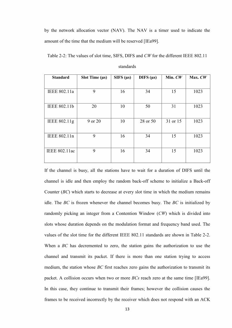
Table 2-2: The values of slot time, SIFS, DIFS and CW for the different IEEE 802.11
standards
Standard Slot Time (µs) SIFS (µs) DIFS (µs) Min. CW Max. CW
IEEE 802.11a 9 16 34 15 1023
IEEE 802.11b 20 10 50 31 1023
IEEE 802.11g 9 or 20 10 28 or 50 31 or 15 1023
IEEE 802.11n 9 16 34 15 1023
IEEE 802.11ac 9 16 34 15 1023
If the channel is busy, all the stations have to wait for a duration of DIFS until the
channel is idle and then employ the random back-off scheme to initialize a Back-off
Counter (BC) which starts to decrease at every slot time in which the medium remains
idle. The BC is frozen whenever the channel becomes busy. The BC is initialized by
randomly picking an integer from a Contention Window (CW) which is divided into
slots whose duration depends on the modulation format and frequency band used. The
values of the slot time for the different IEEE 802.11 standards are shown in Table 2-2.
When a BC has decremented to zero, the station gains the authorization to use the
channel and transmit its packet. If there is more than one station trying to access
medium, the station whose BC first reaches zero gains the authorization to transmit its
packet. A collision occurs when two or more BCs reach zero at the same time [IEa99].
In this case, they continue to transmit their frames; however the collision causes the
frames to be received incorrectly by the receiver which does not respond with an ACK

14
frame. This in turn triggers a re-transmission of the frames by the stations involved.
Therefore, they have to restart the random access process again to reset the BC but the
size of the CW has been doubled. The size of CW is calculated by the Binary
Exponential Back-off Algorithm which is 1 less than an integer power of 2 (i.e. 1, 3,
7…. 511 and 1023). The CW moves to the next greater power of two [IEa09] every time
when the BC is reset as a failed transmission. The CW is reset to the minimum size
when a packet is transmitted successfully, or the associated re-try counter limit is
reached and the packet is discarded. The maximum and minimum sizes allowed for CW
are presented in Table 2-2. This scheme ensures a low delay when only a few station
nodes collide but also ensures that the collision is resolved within an acceptable time
interval when large numbers of station nodes collide.
Figure 2-2 illustrates an example of the operation of the DCF in accessing wireless
medium. There are two station nodes, A and B. After the station node B receives an
ACK and waits a time of DIFS, the channel is idle. Both nodes try to transmit their
packets, so they have to set their back-off counter (BC) values: A is set to 4 and B is set
to 9. The BC of A decreases to zero after 4 time slots have elapsed and can transmit its
packet while B has to freeze its BC at 5 and waits until A completes its transmission.
After a successful transmission A waits for a DIFS time and resets the BC (this time it
has chosen 8) and B just restarts the BC (which is 5). The station node B can transmit its
packet when its BC reaches zero after 5 time slots.

15
Figure 2-2: An example of the DCF operation used to access the medium.
If the channel is idle, the station node has to wait for a time of DIFS and when its back-
off counter (BC) has reached zero before it may transmit its packet. When a packet is
received by the destination node, the destination node has to wait a time of SIFS and
then sends an Acknowledgement (ACK) packet back to the source node to indicate a
successful reception of the data packet. In this thesis, there is a single client station used
in the wireless network of the simulation for the AAM algorithm and the station can
always gain the authorization to use the medium as collisions do not occur as there is no
contention for access. The AAM algorithm is intended for use on a single hop link.
Therefore, it is sufficient to investigate the performance in a single station.
2.3 IEEE 802.11 Frames
In the IEEE 802.11 standards, there are three types of frame defined: Data frame,
Management frame and Control frame.
2.3.1 IEEE 802.11 Data Frame Format
In the IEEE 802.11 standard there are a number of data frame types defined. One way to
classify these data frames are as contention-based service data frames and contention-
free service data frames. The data frame of the contention-free service can only be used
16
in the contention-free period and cannot be used in IBSS (Independent Basic Service
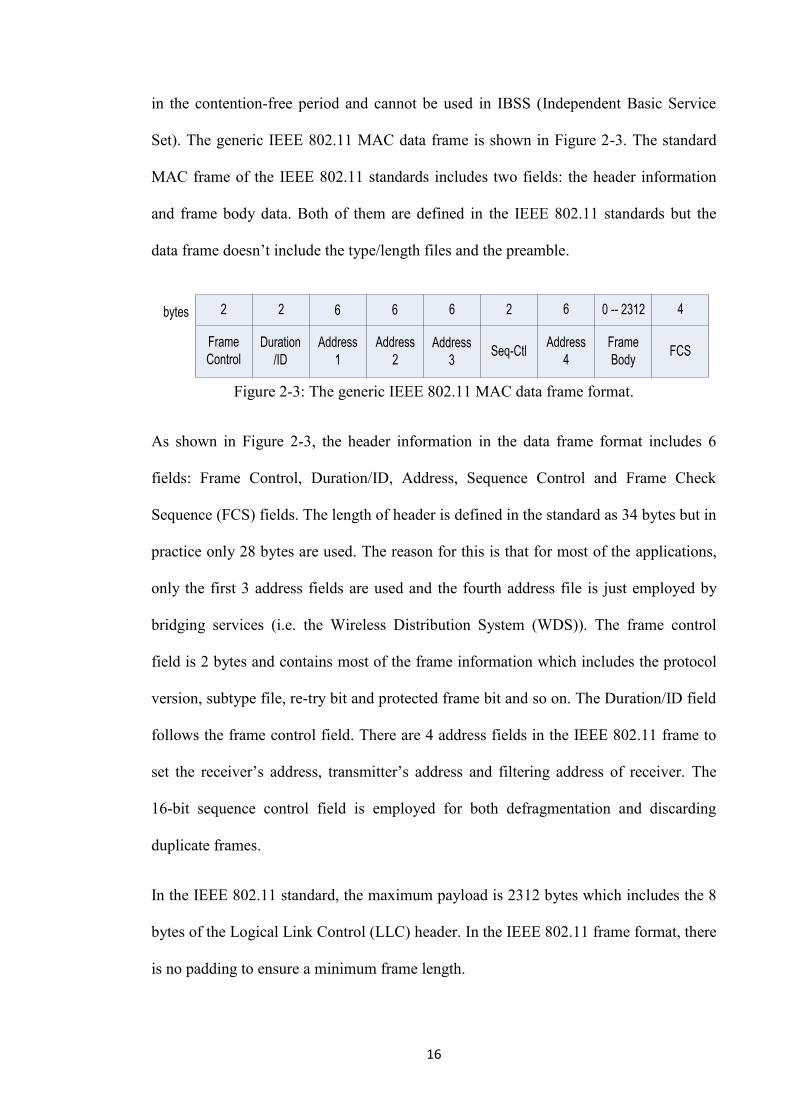
Set). The generic IEEE 802.11 MAC data frame is shown in Figure 2-3. The standard
MAC frame of the IEEE 802.11 standards includes two fields: the header information
and frame body data. Both of them are defined in the IEEE 802.11 standards but the
data frame doesn’t include the type/length files and the preamble.
bytes 2 2 6 6 6 2 6 0 -- 2312 4
FCSFrame
Body
Address
4Seq-Ctl
Address
3
Address
2
Address
1
Duration
/ID
Frame
Control
Figure 2-3: The generic IEEE 802.11 MAC data frame format.
As shown in Figure 2-3, the header information in the data frame format includes 6
fields: Frame Control, Duration/ID, Address, Sequence Control and Frame Check
Sequence (FCS) fields. The length of header is defined in the standard as 34 bytes but in
practice only 28 bytes are used. The reason for this is that for most of the applications,
only the first 3 address fields are used and the fourth address file is just employed by
bridging services (i.e. the Wireless Distribution System (WDS)). The frame control
field is 2 bytes and contains most of the frame information which includes the protocol
version, subtype file, re-try bit and protected frame bit and so on. The Duration/ID field
follows the frame control field. There are 4 address fields in the IEEE 802.11 frame to
set the receiver’s address, transmitter’s address and filtering address of receiver. The
16-bit sequence control field is employed for both defragmentation and discarding
duplicate frames.
In the IEEE 802.11 standard, the maximum payload is 2312 bytes which includes the 8
bytes of the Logical Link Control (LLC) header. In the IEEE 802.11 frame format, there
is no padding to ensure a minimum frame length.
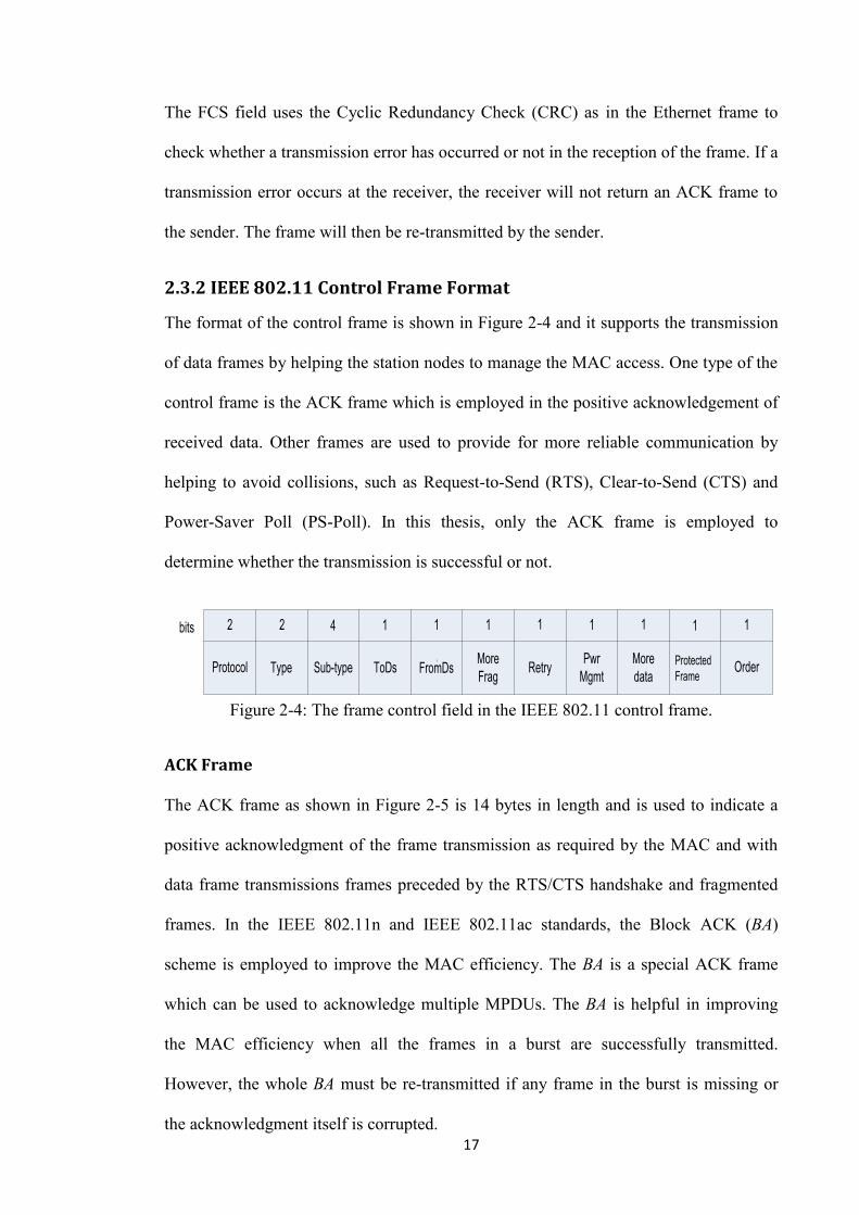
17
The FCS field uses the Cyclic Redundancy Check (CRC) as in the Ethernet frame to
check whether a transmission error has occurred or not in the reception of the frame. If a
transmission error occurs at the receiver, the receiver will not return an ACK frame to
the sender. The frame will then be re-transmitted by the sender.
2.3.2 IEEE 802.11 Control Frame Format
The format of the control frame is shown in Figure 2-4 and it supports the transmission
of data frames by helping the station nodes to manage the MAC access. One type of the
control frame is the ACK frame which is employed in the positive acknowledgement of
received data. Other frames are used to provide for more reliable communication by
helping to avoid collisions, such as Request-to-Send (RTS), Clear-to-Send (CTS) and
Power-Saver Poll (PS-Poll). In this thesis, only the ACK frame is employed to
determine whether the transmission is successful or not.
bits 2 2 4 1 1 1 1 1 1
More
data
Pwr
MgmtRetry
More
FragFromDsToDsSub-typeTypeProtocol
1 1
Protected
FrameOrder
Figure 2-4: The frame control field in the IEEE 802.11 control frame.
ACK Frame
The ACK frame as shown in Figure 2-5 is 14 bytes in length and is used to indicate a
positive acknowledgment of the frame transmission as required by the MAC and with
data frame transmissions frames preceded by the RTS/CTS handshake and fragmented
frames. In the IEEE 802.11n and IEEE 802.11ac standards, the Block ACK (BA)
scheme is employed to improve the MAC efficiency. The BA is a special ACK frame
which can be used to acknowledge multiple MPDUs. The BA is helpful in improving
the MAC efficiency when all the frames in a burst are successfully transmitted.
However, the whole BA must be re-transmitted if any frame in the burst is missing or
the acknowledgment itself is corrupted.
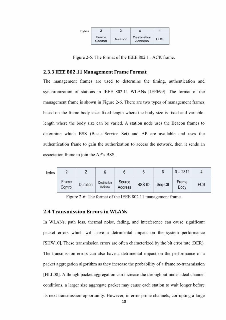
18
bytes 2 2 6 4
FCSDestination
AddressDuration
Frame
Control
Figure 2-5: The format of the IEEE 802.11 ACK frame.
2.3.3 IEEE 802.11 Management Frame Format
The management frames are used to determine the timing, authentication and
synchronization of stations in IEEE 802.11 WLANs [IEEb99]. The format of the
management frame is shown in Figure 2-6. There are two types of management frames
based on the frame body size: fixed-length where the body size is fixed and variable-
length where the body size can be varied. A station node uses the Beacon frames to
determine which BSS (Basic Service Set) and AP are available and uses the
authentication frame to gain the authorization to access the network, then it sends an
association frame to join the AP’s BSS.
bytes 2 2 6 6 6 6 0 -- 2312 4
FCSFrame
BodySeq-CtlBSS ID
Source
AddressDestination
AddressDuration
Frame
Control
Figure 2-6: The format of the IEEE 802.11 management frame.
2.4 Transmission Errors in WLANs
In WLANs, path loss, thermal noise, fading, and interference can cause significant
packet errors which will have a detrimental impact on the system performance
[SHW10]. These transmission errors are often characterized by the bit error rate (BER).
The transmission errors can also have a detrimental impact on the performance of a
packet aggregation algorithm as they increase the probability of a frame re-transmission
[HLL08]. Although packet aggregation can increase the throughput under ideal channel
conditions, a larger size aggregate packet may cause each station to wait longer before
its next transmission opportunity. However, in error-prone channels, corrupting a large

19
size aggregate packet may waste a long period of channel time and leads to a lower
MAC efficiency. So some packet aggregation algorithms [Lin06] [KSP12] have been
proposed to improve the performance in error-prone wireless networks. We will discuss
this in more detail in the next chapter.
2.5 PHY Rate Adaption Mechanisms in WLANs
In the IEEE 802.11 standards, the PHY allows for a set of different transmission modes
to adapt to the channel variations. Each PHY mode uses a specific modulation and
channel coding scheme to offer different performance in terms of throughput. Table 2-3
shows the IEEE 802.11b/g/n PHY rates giving the modulation/coding/MIMO details
where only the IEEE 802.11n mandatory PHY rates are shown and the other IEEE
802.11n PHY rates can be calculated based on the diagram shown in Figure 2-7.
Table 2-3: The details of the PHY rate for IEEE standards 802.11b/g/n.
Standard PHY Rate (Mbps) Modulation Coding Rate MIMO
802.11b 1 DBPSK ---- No
2 DQPSK ---- No
5.5 CCK ---- No
11 CCK ---- No
802.11g 6 BPSK 1/2 No
9 BPSK 3/4 No
12 QPSK 1/2 No
18 QPSK 3/4 No
24 16-QAM 1/2 No
36 16-QAM 3/4 No
48 64-QAM 2/3 No
54 64-QAM 3/4 No
802.11n
(mandatory PHY rate)
6.5 BPSK 1/2 1
13 QPSK 1/2 1
19.5 QPSK 3/4 1
26 16-QAM 1/2 1
39 16-QAM 3/4 1
52 64-QAM 2/3 1
58.5 64-QAM 3/4 1
65 64-QAM 5/6 1
Where, DBPSK: Differential Binary phase-shift keying; DQPSK: Differential
Quadrature phase-shift keying; CCK: Complementary Code Keying; QAM: Quadrature

20
amplitude modulation; 16-QAM: 16-state quadrature amplitude modulation; 64-QAM:
64-state quadrature amplitude modulation.
New 11n PHY
Rate
Choose one
11n Mandatory
PHY Rate
Optionally
multiply the
number of
additional
spatial streams
(2,3,or 4)
Optionally
multiply 2.077
to bond two
20MHz
channels
Optionally
multiply by 1.1
for shorter
Guard Interval
to increase
symbol rate
Figure 2-7: Calculating the new IEEE 802.11n PHY rate.
The PHY rate adaption is the process of dynamically switching the PHY mode to match
the channel conditions. The goal is to select the most effective rate that will achieve the
maximum throughput for a given channel condition [HVB01]. The effect of
transmission errors also impacts on the selection of PHY rate for transmission. There
are many PHY rate adaption mechanisms that have been proposed, such as [HVB01]
[KaM97] [WYL06] [MLT08], to achieve the goal of realizing a maximum throughput
in error-prone wireless network channels.
The PHY rate adaption mechanism can reduce the number of re-transmissions caused
by the transmission errors. The ARF (Auto Rate Fallback) [KaM97] mechanism is a
simple and widely adopted scheme which is based on the number of consecutive
successful or unsuccessful transmission attempts to determine whether to increase or
decrease the transmission rate. The disadvantage of the ARF mechanism is that it tries a
higher transmission rate every time after it successfully transmits a fixed number of
packets even if the current rate is the most effective rate to achieve the maximum
throughput. The AARF (Adaptive ARF) mechanism is proposed to alleviate this
problem [WYL06]. The AARF mechanism behaves like the ARF mechanism except
that the number of consecutive successfully transmission attempts is exponentially
incremented when the higher transmission rate has failed. In the Receiver Based Auto
21
Rate (RBAR) mechanism the RTS/CTS handshake is mandatory and the RTS, CTS
frames structure has been modified [HVB01]. The Robust Rate Adaption Algorithm
[MLT08] mechanism is composed of the rate selector mechanism and the adaptive RTS
mechanism which does not always make the best choice for the rate [YWA04] as the
rate selected depended on the used rate. In this thesis, we use the popular AARF
mechanism to select the PHY rate in an error-prone wireless network.
2.6 Network Simulators
A network simulator is an important research tool in which a computer program
simulates the behavior of a network either by calculating the interaction between the
different network entities using mathematical formulas or by actually capturing and
playing back observations from a live network. It models the behaviors of the network
and the various applications and services which can be observed in a test laboratory.
Various attributes of the environment can also be modified in a controlled manner to
assess how the network would behave under different conditions.
There are a number of network simulators available such as OPNET, GloMoSim, ns-2
and ns-3 etc. OPNET is a commercial software package for analyzing the performance
of computer networks and applications. GloMoSim is another popular network
simulator tool that is employed for network research and laboratory experimentation
and covers many technologies. The network simulator (ns) has a long history and is
derived from REAL (Real and Large). It (i.e. ns) is a name for a series of discrete event
network simulators particularly ns-1, ns-2 and ns-3. They are free open source discrete-
event network simulators primarily used in research and teaching [TNS12]. The ns-1,
the first version of ns, was developed at Lawrence Berkeley National Laboratory
(LBNL) between 1995 and 1997. The second version of ns, called ns-2, was based on a
refactoring by Steve McCanne in 1996-1997 [BBE99].
22
The network simulator ns-3 [BEF00] is the third generation of this family of network
simulators. The project started in 2006 and is still being actively developed today. It is
not an extension of ns-2 and does not support the APIs (Application Program Interface)
from ns-2, but some modules of ns-2 have been ported to ns-3 [NS312]. The ns-3 is a
new simulator and built on C++ and Python. It is essentially a C++ library where many
network simulation modules are implemented as C++ objects and are wrapped by
Python. Normally, the C++ or Python applications can instantiate a set of simulation
modules to set up the simulation scenario of interest, enter the simulation main loop,
and exit when the simulation is completed. It provides support for TCP/UDP, routing,
and most of the IEEE 802 standards for wired and wireless networks.
The advantages of ns-3 over other discrete-event network simulators are as follows
[NS313]: (i) It uses the object oriented language C++ and Python which allow the user
to take advantages of the full support from each language. (ii) The callback-driven
events scheme is used to make it easy to turn any function into an event and be
scheduled. In fact, the simulation events in ns-3 are simply function calls that are
scheduled to execute at a prescribed simulation time. (iii) Different levels of user
flexibility. It allows the expert user to configure the core from the low-level APIs which
are powerful and the normal users to configure it from invoking the high-level easier-to-
use APIs. (iv) An emphasis on simulation that allows the simulator to interact with the
real world. Several different simulation-in-the-loop and virtual machine integration
frameworks have been developed. (v) Alignment with real-world interfaces where
objects (e.g. sockets, net devices) are aligned with those in a Linux computer which
facilitates code reuse and improves the realism of the models and makes the simulator
control flow easier compared to real system. (vi) Configuration management is
developed which uses an integrated attribute-based system to manage default and per-
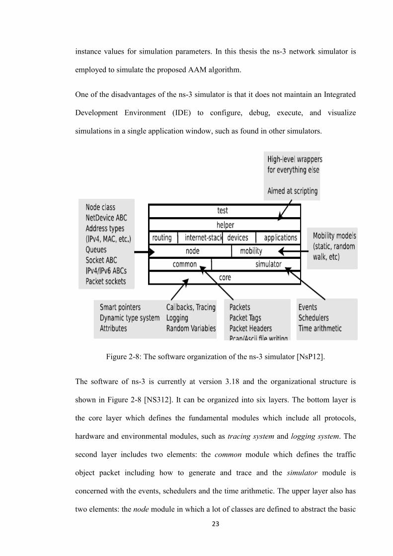
23
instance values for simulation parameters. In this thesis the ns-3 network simulator is
employed to simulate the proposed AAM algorithm.
One of the disadvantages of the ns-3 simulator is that it does not maintain an Integrated
Development Environment (IDE) to configure, debug, execute, and visualize
simulations in a single application window, such as found in other simulators.
Figure 2-8: The software organization of the ns-3 simulator [NsP12].
The software of ns-3 is currently at version 3.18 and the organizational structure is
shown in Figure 2-8 [NS312]. It can be organized into six layers. The bottom layer is
the core layer which defines the fundamental modules which include all protocols,
hardware and environmental modules, such as tracing system and logging system. The
second layer includes two elements: the common module which defines the traffic
object packet including how to generate and trace and the simulator module is
concerned with the events, schedulers and the time arithmetic. The upper layer also has
two elements: the node module in which a lot of classes are defined to abstract the basic
24
computing device and the mobility module that provides the library to support node
mobility. The fourth layer is concerned with routing, device and application modules.
The fifth is the helper module which provides a set of APIs to help to interact with all
other modules. The top layer is the test module which contains test cases to allow the
user to test the system or modules.
In this thesis, the wifi module in the core layer has been modified to include the
proposed AAM algorithm and the basic simulation setup for packet aggregation in ns-3
is shown in Figure 2-9. It shows the basic processes required in sending and receiving
an aggregate packet to and from another node in a wireless node. For example, to send
an aggregate packet from the source node to another node requires the following steps.
At first, the packet generator is used to generate the packets. In our simulation, the
module OnOffApplication is used to generate the required packets which have the same
key characteristics (e.g. length, destination IP address) as real world packets. Then the
WifiNetDevice pushes these packets into the WifiMacqueue in the MAC. After gaining
the authorization to transmit a packet, the EdcaTxopN module invokes the
MsduStandardAggregator/MsduAggregator to combine packets from the queue. If
required, the PHY rate is selected by the PHY rate adaption modules (e.g.
AarfWifiManager) to send the aggregate packet. Transmission errors can also be
included by employing some modules (e.g. NistErrorRateModel). Then the aggregate
packet is sent through the WifiChannel module which is set by the WifiPhy module.
Having finished the transmission, it waits for the ACK frame. If it does not receive the
ACK frame, the frame is re-transmitted by the MacRxMiddle module if required. If it
receives the ACK, the transmission is successful. This is the basic transmission
aggregate packet process. We just selected the most suitable modules (e.g.
AarfWifiManager, NistErrorRateModel) to implement the algorithm in our simulations.

25
We also modified some of these modules to implement some new functions which will
be described further in chapter 4.
Packet Generator
(OnOffApplication)
WifiNetDevice
StaWifiMAC
(WifiMAcQueue)
EdcaTxopN
(MsduStandardAggregator)
MacLow
(AarfWifiManager)
WifiPhy
(NistErrorRateModel)
WifiChannel
DcfManager
Listener
Listener
Packet Receiver
(PacketSink)
MAcRxMiddle
MacLow
WifiPhy
StaWifiMAC
Send Packet Receive Packet
WifiNetDevice
Figure 2-9: Basic simulation of packet aggregation in ns-3.
2.7 Packet Sniffers
A packet sniffer is a program running on a network attached device that passively
receives frames passing through the device’s network adapter [ARC02]. A packet
sniffer is also known as a Network Analyzer or Protocol Analyzer or Wireless Sniffer.
The packet sniffer can monitor all data transmitted on the network and save it for
analysis later. The packet sniffer can be used as an administrative tool to monitor and
troubleshoot network traffic [AGS03]. Figure 2-10 shows a typical packet sniffer
program running in a wireless network.
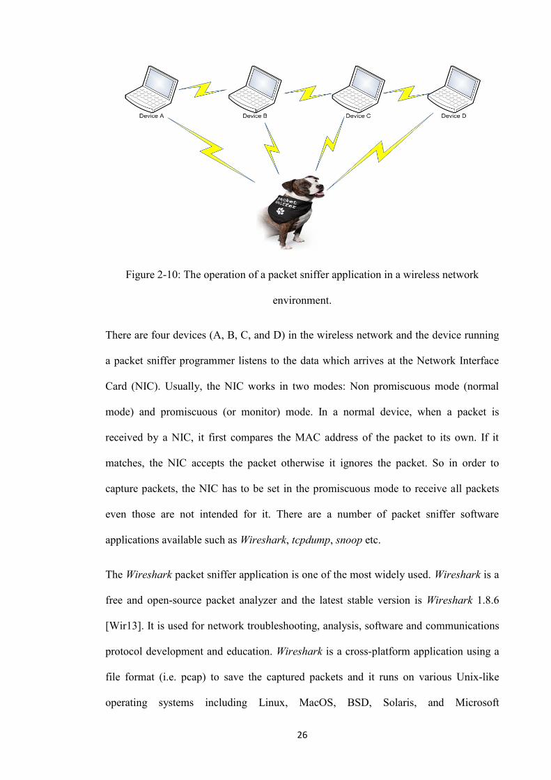
26
Figure 2-10: The operation of a packet sniffer application in a wireless network
environment.
There are four devices (A, B, C, and D) in the wireless network and the device running
a packet sniffer programmer listens to the data which arrives at the Network Interface
Card (NIC). Usually, the NIC works in two modes: Non promiscuous mode (normal
mode) and promiscuous (or monitor) mode. In a normal device, when a packet is
received by a NIC, it first compares the MAC address of the packet to its own. If it
matches, the NIC accepts the packet otherwise it ignores the packet. So in order to
capture packets, the NIC has to be set in the promiscuous mode to receive all packets
even those are not intended for it. There are a number of packet sniffer software
applications available such as Wireshark, tcpdump, snoop etc.
The Wireshark packet sniffer application is one of the most widely used. Wireshark is a
free and open-source packet analyzer and the latest stable version is Wireshark 1.8.6
[Wir13]. It is used for network troubleshooting, analysis, software and communications
protocol development and education. Wireshark is a cross-platform application using a
file format (i.e. pcap) to save the captured packets and it runs on various Unix-like
operating systems including Linux, MacOS, BSD, Solaris, and Microsoft

27
Windows[ThW12]. The Wireshark not only captures network packets but also displays
the captured packet data in a detailed format where an example is shown in Figure 2-11.
In this thesis, the simulation is based on 16 traffic trace files which were captured by the
wireshark from a number of different live Wi-Fi hotspot networks at different times and
locations and whose details will be described in chapter 4.
Figure 2-11: An example of how Wireshark captures packets and parses their contents.
2.8 Chapter Summary
In this chapter, we have introduced the development and general concepts of the IEEE
802.11 WLANs including the structure of MAC frames, transmission errors and PHY
rate adaption mechanisms in WLANs, network simulators and packet sniffer
applications. The architecture of the wireless network was presented which is the main
network topology used to implement the proposed AAM algorithm. A number of the
IEEE 802.11 standards and the main components of WLANs were discussed and the
typical network topology was shown. In particular, the IEEE 802.11n and IEEE
802.11ac standards were introduced which support the packet aggregation algorithm

28
and proposed two packet aggregation algorithms (i.e. A-MSDU and A-MPDU) whose
details will be described in the next chapter. The MAC mechanism of the IEEE 802.11
standard was presented and the details of how to access the medium, inter-frame times
and the back-off contention scheme were also introduced. The impact of transmission
errors and various PHY rate adaption mechanisms were discussed.
Network simulation tools are important tools to research the performance of network
algorithms, protocols and environments. There are currently a number of free open
source simulation tools available for researchers. One of the network simulation tools is
the ns-3 which is still under developing and has a number of advantages. The ns-3 is
employed in this thesis to implement and simulate the operation of the proposed AAM
algorithm. The packet sniffer was presented in this chapter and the Wireshark software
application was also introduced.
29
Chapter 3 Review of Packet Aggregation
Algorithms
In this chapter a number of packet aggregation algorithms proposed for wireless
networks will be presented. In particular we will attempt to describe what research is
being carried out in the development of packet aggregation algorithms targeted at
wireless networks. As will be shown, current approaches failed to achieve the goal of
realizing an optimal trade-off between maximizing throughput and minimizing delay
which is concerned with improving maximum throughput at the cost of the least delay
increase. The majority of current researchers are only concerned with optimizing a
single metric algorithm which attempts to achieve the goal of either maximizing
throughput or minimizing delay. For these algorithms, they don’t take account of the
varying nature of mixed traffic loads. Some algorithms can achieve large throughputs at
the expense of large delays while others achieve the goal of minimizing delay
associated with small throughputs. Throughput and delay are the two most important
performance metrics used to analyze a packet aggregation algorithm.
3.1 Throughput and Delay
3.1.1 Throughput
In modern communication networks such as WLANs or Ethernet networks, the
throughput or network throughput is the average rate at which data is successfully
transmitted through a communications channel [Rap02]. In general, throughput is
measured in bits per second (bps) or it can sometimes be measured in packets per
second (pps). In this thesis the throughput is defined as the average payload in bits
successfully transmitted in unit time from the source node to the destination node in a
wireless network.

30
The maximum throughput of a network is important for both user and system designer
as it is essentially synonymous with the capacity of the network. The maximum
throughput can be defined in a number of different ways such as the maximum
achievable throughput, the peak measured throughput or the maximum sustained
throughput. In this thesis, we define the maximum average throughput as the average
throughput under saturation conditions in wireless networks.
For the IEEE 802.11 wireless networks, Xiao and Rosdahl [XiR02] [XiR03] showed
that a throughput upper limit (TUL) exists. The TUL of wireless network is defined in
[XiR02] and the authors assumed a wireless network where one sender and one receiver
operate in the DCF mode. The sender always has packets to be transmitted and each
packet has the same size. This throughput is determined at the Link Layer Control. It is
assumed that there are no transmission errors present in order to emphasize the impact
of the overheads which includes the PLCP (Physical Layer Convergence Protocol)
preamble and the PLCP header. The TUL is given by the following equation:
…… (3.1)
Where denotes the payload of the packet in bytes, denotes the transmission
time of the PLCP preamble, denotes the transmission time of the PLCP header,
is the time of DIFS, is the time of SIFS, is the minimum size of
contention window in unit of a slot time, is the time duration of a slot time and is
the propagation delay that is the propagation time between the nodes by the radio signal
which usually can be ignored as its value is negligible compared to that of other times.
The distance between wireless nodes is less than 50 meters, so the time of propagation
is less than 0.2 μs. The values of the parameters are shown in Table 3-1 for the IEEE
802.11a, IEEE 802.11b, IEEE 802.11n and IEEE 802.11ac standards.

31
Table 3-1: The PHY parameter values for some of the IEEE 802.11 standards
Parameter IEEE
802.11 a
IEEE
802.11 b
IEEE
802.11 n
IEEE
802.11 ac Comment
Tslot 9 μs 20 μs 9 μs 9 μs slot time
TDIFS 34 μs 50 μs 34 μs 34 μs DIFS duration time
CWmin
15 31 15 15
Minimum contention
window size in unit of
slot time
Tp 16 μs 144 μs
16 μs 16 μs PLCP preamble
duration
TPHY 4 μs 48 μs 4 μs 4 μs PLCP header duration
TSIFS 16 μs 10 μs 16 μs 16 μs SIFS duration time
τ 1 μs 1 μs 1 μs 1 μs Propagation delay
Figure 3-1: The throughput against data rate without packet aggregation [Hud09].
The TUL is defined as the maximum throughput when the PHY rate increases
indefinitely. As shown in Figure 3-1, for a certain PHY rate, the throughput is almost
independent of data rate when packets have a fixed size [Hud09]. This is due to the
large amount of overhead added to every packet. This suggests that there are two
32
methods to improve the throughput by increasing the average size of payload or
specifically by reducing the ratio of header size to payload size in a frame. Both
methods can be achieved by using a packet aggregation algorithm which is why packet
aggregation algorithms have become so popular. For example, the latest IEEE 802.11n
standard and the IEEE 802.11ac standard (which is still under development) support the
use of packet aggregation. There are two packet aggregation algorithms proposed in the
IEEE 802.11n standard namely Aggregate MAC Service Data Unit (A-MSDU) and
Aggregate MAC Protocol Data Unit (A-MPDU) which will be described in section 3.3.
3.1.2 Delay
Network delay in wireless networks specifies how long it takes for a data packet to
travel across the wireless network from one node to another. It is an important
performance characteristic of an IEEE 802.11 wireless network. The network delay is
usually divided into several parts depending on the location of the specific pair of
communicating nodes: processing delay, queuing delay, transmission delay and
propagation delay. In this thesis, the delay is defined as the average time to successfully
transmit a packet from the MAC layer of the source node to the MAC layer of the
destination node in wireless networks and the minimum average delay is defined as the
average delay under saturation conditions in wireless networks.
There is a certain minimum level of delay which will be experienced due to the time it
takes to transmit a packet serially through a link [ZNN10]. The delay lower limit (DLL)
of the DCF model in the IEEE 802.11 wireless network is derived in [XiR02] [QCS02].
To derive the DLL, the system needs to be operated under a best-case scenario: (i) The
channel is an ideal channel without transmission errors present; (ii) At any transmission
cycle, there is one and only one active station which always has packets to send and
33
other stations can only receive packets and provide acknowledgements (ACKs). The
DLL is given by equation (3.2) [XiR02].
……… (3.2)
Where all of the parameters have been defined as in equation (3.1) and their values are
given in Table 3-1. This DLL does not consider the queuing time and waiting time at
the MAC.
3.1.3 Discussion of Throughput and Delay
So far, we have introduced the concepts of the throughput and the delay, and also
defined how they are used in the analysis of the proposed AAM algorithm. In WLANs,
an upper limit on the throughput exists and is given by [XiR02] [XiR03] [QCS02]. Due
to the protocol overhead associated with the transmission packet, the throughput cannot
be further increased without reducing the protocol overheads even though the data rate
increases indefinitely. A packet aggregation algorithm is used to reduce the average
protocol overhead and can significantly improve the throughput. Also a lower limit on
the delay in wireless networks exists and is defined by [XiR02] [QCS02] where the
delay of both the queuing time and waiting time in the MAC are not considered.
However, the time spent waiting for more packets to arrive is the main delay for the
packet aggregation algorithm [TYH10]. Therefore, there is a trade-off in terms of an
increased throughput and an increased delay when employing a packet aggregation
algorithm. This trade-off will be discussed in the next section.
3.2 Trade-off between Throughput and Delay
As discussed in the last section, throughput is the key metric that packet aggregation
algorithms try to improve. Reducing the protocol overheads is an important approach to
improving the throughput as an upper limit on throughput exists. Studies have shown

34
that the packet aggregation can significantly improve the throughput. For example,
adopting a packet aggregation algorithm in [KGL06] increases by a factor of 7 the
number of calls that can be supported for VoIP applications; [JDB10] improves the
throughput by a factor of 2.5 times; and [MaA12] achieves a 200% improvement in the
throughput.
However, the delay can also be increased as the throughput increases when packet
aggregation algorithms are employed. The existence of a delay lower limit has been
defined and demonstrated in wireless networks by [XiR02]. But the delay lower limit
does not consider the queuing delay and waiting delay both of which are the dominant
delay components that are increased when using a packet aggregation algorithm. We
will describe the delay associated with a packet aggregation algorithm.
3.2.1 Delay Associated with a Packet Aggregation
Delay is the key cost associated with the use of a packet aggregation algorithm to
improve the throughput. There have been many studies conducting regarding the delay
associated with packet aggregation in wireless networks.
In [Lin06], a model was proposed to calculate the packet aggregation delay. This model
studies error-prone channels using A-MPDU and A-MSDU packet aggregation
algorithms both of which are popular packet aggregation algorithms defined in the IEEE
802.11n standard and will be described in the next sections. In this model, the network
saturation throughput is defined based on a wireless network where M station nodes use
the RTS/CTS scheme to access the same channel. The network saturation throughput (S)
is given by equation (3.3).
………………………………………….. (3.3)
35
Where, is the successfully transmitted payload size (in bits) in unit time, is the
expected length of the time slot, which is defined as the time when a station starts to
check the channel state (i.e. idle or busy) for transmitting a packet until it receives an
ACK of the packet. As there are M station nodes competing for transmission, the
average access delay is given by equation (3.4)
………………………..……………. (3.4)
Where is the aggregate packet size (in bits). The simulation results show that the
delay increases as the BER increases for the packet aggregation algorithm. This delay
only considers the transmission delay and does not include other components such as
queuing time.
In [TYH10], a delay calculation is proposed which calculates the delay of a packet’s life
time and is the first work focusing on packet delay of packet aggregation algorithm. The
average delay ( ) of a packet includes two parts: the queuing delay ( ) and the
transmission delay ( ) which equals the value of delay ( ) in the equation (3.4).
………….……………………..… (3.5)
………………..………..……………….… (3.6)
If the length of MAC queue is in bytes where it assumes that the queue is always full,
and the aggregate packet size is bytes which are transmitted at each period, the
queuing delay is shown in (3.7)
……………….………..…………. (3.7)
From the equations (3.4), (3.5), (3.6) and (3.7), the average delay ( is given by (3.8)
36
…………….…..…………... (3.8)
This results show that the average delay is affected by the BER, the aggregate packet
size and the number of competing nodes. As the BER and the number of competing
nodes cannot be controlled, one way that the delay can be changed is to adjust the
aggregate packet size.
The packet aggregation algorithm proposed in [ZIF08] is based on the Packet
Reservation Multiple Access (PRMA) protocol. In this model, the PRMA data
transmission is based on the Markov chain model and it assumes that the aggregation
process starts after the arrival of a certain number of packets into the buffer. In [ZIF08],
the packet aggregation delay is the delay experienced by the first arrival packet (i.e. the
time from when it arrives at a terminal’s buffer until the time it can start to be
transmitted). The delay consists of two parts: packet aggregation delay and channel
access delay. The packet aggregation delay is the queuing time of the first arrival packet
waiting in the buffer, so the mean aggregation delay is given based on the Markov chain:
………….……....… (3.9)
Where α denotes the average packet transmission period, denotes the packet arrival
rate. As discussed in [ZIF08], a number of conclusions have been drawn: (i) The
aggregate packet has a long packet aggregation delay when the packet arrival rate is low,
this means that the first arrival packet could wait a longer time in the buffer for the size
of packets in the buffer to exceed the specified target aggregate packet size; (ii) With a
fixed arrival rate, the aggregate packet has a higher aggregation delay with a bigger
target aggregate packet size; (iii) The proposed algorithm cannot achieve throughput
gains by packet aggregation algorithm at the expense of high delay when the packet

37
arrival rate is low; (iv) There is a trade-off between throughput and delay when using
packet aggregation. As the packet arrival rate is unpredictable, the packet aggregation
delay is controlled by the target packet aggregation size.
3.2.2 Trade-Off between Throughput and Delay
It is clear that packet aggregation algorithms can significantly improve the throughput
but any improvement will also have an associated cost in terms of a delay increase. As a
delay lower limit and a throughput upper limit exist in the IEEE 802.11 wireless
networks, most of the proposed packet aggregation algorithms try to asymptotically
approach these limits.
Most of the proposed packet aggregation algorithms attempt to optimize a single metric,
i.e. either to maximize throughput or to minimize delay. For example, for time sensitive
applications (e.g. VoIP, video streams), the packet aggregation algorithms focus on the
delay, such as in [TYH10] [KuD06]. For some other applications, such as E-mail, they
can tolerate a relatively longer delay than time sensitive applications. They focus on the
improvement in throughput by using packet aggregation algorithms. However, for a
significant number of wireless networks, the traffic load is mixed containing many
different types of applications that can have very different network performance
requirements. It requires that the packet aggregation algorithm should be adaptive to
achieve an optimal trade-off between throughput and delay. The adaptive algorithm
should be capable in improving the maximum throughput with the least cost in terms of
a delay increase.
An aggregation algorithm has a superior performance over other algorithms in terms of
the trade-off between maximizing throughput and minimizing delay if it can deliver a
throughput greater than that of other algorithms for a given delay increase. This is
illustrated in Figure 3-2 where there are two packet aggregation algorithms A and B
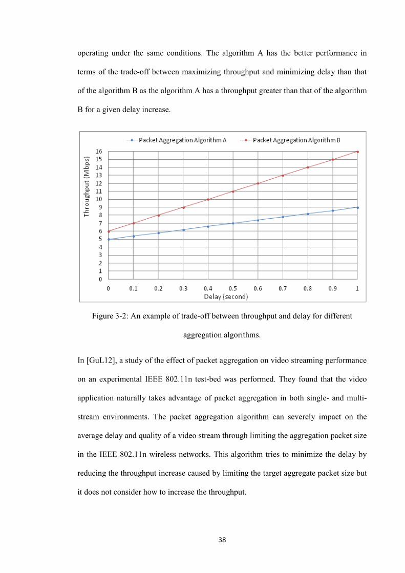
38
operating under the same conditions. The algorithm A has the better performance in
terms of the trade-off between maximizing throughput and minimizing delay than that
of the algorithm B as the algorithm A has a throughput greater than that of the algorithm
B for a given delay increase.
Figure 3-2: An example of trade-off between throughput and delay for different
aggregation algorithms.
In [GuL12], a study of the effect of packet aggregation on video streaming performance
on an experimental IEEE 802.11n test-bed was performed. They found that the video
application naturally takes advantage of packet aggregation in both single- and multi-
stream environments. The packet aggregation algorithm can severely impact on the
average delay and quality of a video stream through limiting the aggregation packet size
in the IEEE 802.11n wireless networks. This algorithm tries to minimize the delay by
reducing the throughput increase caused by limiting the target aggregate packet size but
it does not consider how to increase the throughput.
39
In [Wla12], the authors proposed a new model to obtain the optimal packet aggregation
size with regard to the delay constraints of nodes. This model specifies a parameter for
the time limit of a node to access the channel which means that the node cannot wait a
longer time than this to access the channel. The simulation results show that the delay
increases with an increase in the number of nodes attempting to access the channel for
the normal IEEE 802.11n scheme and the delay is less than the value of the specified
parameter. The idea of this scheme is different to that of the previous schemes. This
scheme attempts to fix the upper limit of delay to control the average packet delay,
while the previous scheme (i.e. [GuL12]) attempts to limit the packet aggregation size
to achieve the goal. In other words, the proposed algorithm in [Wla12] bounds the delay
increase at the cost of limiting the throughput increase. In particular, if there are a large
number of nodes attempting to transmit in a wireless network, the throughput is not
increased and may even be decreased under the proposed scheme compared to that of
non-aggregation.
In [ZIF08], the authors found that the packet arrival rate is an important factor that
affects the delay: the higher the packet arrival rate the shorter the waiting time in the
buffer and the smaller the delay. However, in practice the packet arrival rate is
essentially random and uncontrollable. So there is a need to develop adaptive packet
aggregation algorithms that are better suited to the variations in the packet arrival rate.
In this thesis, we investigate the performance of the proposed AAM algorithm in terms
of the aggregation trade-off where the aggregation trade-off is defined as the maximum
average throughput with the minimum average delay in wireless networks.
3.2.3 Discussion of Trade-off between Throughput and Delay
In this section, we discuss the trade-off between the throughput and the delay when
employing a packet aggregation algorithm in wireless networks. Generally, the

40
throughput is improved at the expense of a delay increase. In modern networks the
traffic load is a mix of different types of applications which can have very different
requirements in terms of network performances. Therefore there is a requirement to
realize some form of an optimal trade-off between maximizing throughput and
minimizing delay.
There are a number of factors that impact the throughput and the delay, such as target
aggregate packet size, channel noise, contention for access etc. But there is one factor
that is the target aggregate packet size which can be controlled to manage both
throughout and delay. The others are essentially unpredictable and uncontrollable, such
as the packet arrival rate and transmission errors. Generally, the larger the size of the
aggregate packet, the higher the throughput but also the larger the delay as it may wait
longer for packets to arrive. Therefore many researchers have attempted to achieve the
goal of finding the optimal packet aggregation size that minimizes the delay and
maximizes the throughput.
As it is difficult to achieve the optimal trade-off for mixed traffic loads by using packet
aggregation algorithm, some studies are only focused on some special applications, such
as VoIP or video streaming. In this thesis, the proposed AAM algorithm is used to
achieve the best aggregation trade-off in terms of achieving the maximum average
throughput with the minimum average delay for different traffic loads in wireless
networks.
3.3 Packet Aggregation Algorithms
It is clear that increasing the data rate or changing the modulation scheme can improve
the performance in terms of throughput in IEEE 802.11 WLANs. However, due to the
IEEE 802.11 protocol overheads (e.g. MAC header), a throughput upper limit (TUL)
exists which was shown by Xiao and Rosdahl [XiR02] [XiR03]. The MAC is inefficient

41
due to the MAC protocol headers, back-off time, inter-frame spacing and ACKs, and
this inefficiency is the most pronounced when the data rate is high or the payload is
small. To achieve higher throughputs it is necessary to reduce protocol overheads
particularly for small size packets. The protocol overhead is the key factor for small
sized packet to lower the MAC efficiency which is clearly demonstrated by Dionysius
et al. [SNC08]. The idea of packet aggregation algorithm was proposed by Shaffer
[SWC99] in 1999 and Gopalakrishna [Gop03] proposed their packet aggregation
method in 2003. A lot of research has been conducted to show how packet aggregation
can improve the throughput in wireless networks. D. Skordoulis [SNC08] has
demonstrated the influence of aggregation, block acknowledgement on the throughput
of the IEEE 802.11 WLANs. In [BMS09], the study shows that the packet aggregation
algorithm has significantly improved the throughput for the various application data
traffic in an IEEE 802.11 experiment test-bed.
Packet aggregation is shown in Figure 3-3 where there are three packets aggregated into
a single packet at the sender. This reduces the number of MAC headers required from
three to just one header. The two MAC headers do not need to be transmitted which
represents a saving of two MAC overheads.
Figure 3-3: The aggregation process for packet aggregation algorithm in wireless
networks.

42
Packet aggregation algorithms can be divided into different classes based on the
different strategies employed. For example, in [HeC04], the packet aggregation may be
performed at different granularities: aggregating all the packets (full aggregation),
aggregating packets from the same traffic class (per-class aggregation) and aggregating
packets from the same flow (per-flow aggregation). While, there are eight ways to
classify them as proposed in [Xia05]: (i) distributed vs. centrally controlled; (ii) ad-hoc
vs. infrastructure; (iii) uplink vs. downlink; (iv) single-destination vs. multi-destination;
(v) PHY-level vs. MAC-level; (vi) single-rate vs. multi-rate; (vii) immediate ACK vs.
delay ACK; (viii) no spacing vs. SIFS spacing.
In this thesis, the different aggregation algorithms will be divided into 4 categories
based upon the aggregation discipline and selection strategy employed. The aggregation
packet selection strategy describes the way in which the packets are selected for
assembling. The two categories here are first-in first-out (FIFO) and Non-FIFO. The
FIFO discipline selects the packets based on the time of arrival into the buffer which is
also the benchmark algorithm used here to compare with the proposed AAM algorithm.
Non-FIFO uses other methods to select the packets.
The aggregation discipline can either be fixed or adaptive depending on whether the
algorithm parameters are fixed or are dynamically adjusted in response to variations in
the network conditions. Combining these two approaches results in 4 categories for
aggregation algorithms: (1) Fixed with FIFO selection strategy (FF); (2) Fixed with
Non-FIFO selection strategy (FNF); (3) Adaptive with FIFO selection strategy (AF); (4)
Adaptive with Non-FIFO selection strategy (ANF).
3.3.1 Fixed with FIFO Packet Aggregation Algorithms (FF)
The FF packet aggregation algorithm does not automatically adjust the parameters of
the algorithm to adapt to the variations in network conditions and uses the FIFO
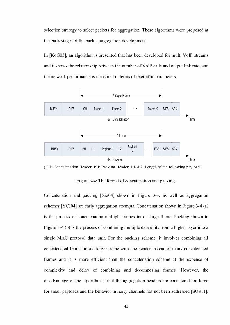
43
selection strategy to select packets for aggregation. These algorithms were proposed at
the early stages of the packet aggregation development.
In [KoG03], an algorithm is presented that has been developed for multi VoIP streams
and it shows the relationship between the number of VoIP calls and output link rate, and
the network performance is measured in terms of teletraffic parameters.
…
(a) Concatenation Time
(b) Packing Time
BUSY DIFS PH L 1 Payload 1 L 2Payload
2…... FCS SIFS ACK
BUSY DIFS CH Frame 1 Frame 2 Frame K SIFS ACK
A Super Frame
A frame
(CH: Concatenation Header; PH: Packing Header; L1~L2: Length of the following payload.)
Figure 3-4: The format of concatenation and packing.
Concatenation and packing [Xia04] shown in Figure 3-4, as well as aggregation
schemes [YCJ04] are early aggregation attempts. Concatenation shown in Figure 3-4 (a)
is the process of concatenating multiple frames into a large frame. Packing shown in
Figure 3-4 (b) is the process of combining multiple data units from a higher layer into a
single MAC protocol data unit. For the packing scheme, it involves combining all
concatenated frames into a larger frame with one header instead of many concatenated
frames and it is more efficient than the concatenation scheme at the expense of
complexity and delay of combining and decomposing frames. However, the
disadvantage of the algorithm is that the aggregation headers are considered too large
for small payloads and the behavior in noisy channels has not been addressed [SOS11].

44
In [YCJ04], the performance of frame aggregation is evaluated by both numerical
analysis and experimental measurements obtained from a test-bed. According to the
measurement results, the frame aggregation can improve the throughput performance of
the IEEE 802.11b WLAN by 2 to 3 Mbps, when multiple frames are aggregated.
However, it does not consider the delay.
There has been renewed interested in their applications for wireless networks [KGL06]
[RLI06], where fairness and inefficiency issues in the IEEE 802.11-based wireless
systems are examined. In [KGL06], a distributed packet aggregation algorithm is
proposed for Voice over IP (VoIP) used in multi-hop wireless networks. The
experimental results demonstrate that the number of calls supported increases to 8 for
the proposed aggregation algorithm compared to 1 in the case of no aggregation. The
disadvantage of the proposed algorithm is that it only operates for a single application,
i.e. VoIP. VoIP is one of the most important applications to be researched in the
development of packet aggregation algorithms as the average size of a VoIP packet is
small. However it imposes a constraint on the maximum delay allowed, typically less
than 150 ms [ITU03]. Normally, the packet aggregation algorithms for the time
sensitive applications (e.g. VoIP or video streaming) are focused on the increased delay
resulting from an improvement the throughput.
In [Hud09], a scheme called the frame aggregation and block acknowledge (FABA) is
proposed which is shown to be capable of providing a throughput that is sufficient for
multimedia applications, even at rates of over 100 Mbps. FABA combines the packet
aggregation mechanism and the block acknowledgement mechanism to improve the
throughput. In this scheme, a number of aggregate packets will be transmitted from the
sender in a single back-off period and a special ACK frame will be sent to the sender
45
from the receiver. However, it is based on a new MAC scheme designed by the author
and not easily implemented.
In [LNM09] [MaE07], the authors proposed a scheme called Aggregation and Fragment
Retransmission (AFR) scheme to aggregate as many packets as possible into a large
frame. This large frame is, in turn, fragmented into smaller fragments before being
transmitted. If transmission errors occur during the transmission, only the corrupted
fragments of the large frame are re-transmitted. The simulation results show that AFR
achieves between 2.5 and 3 times the throughput of DCF over a range of network
conditions for TCP traffic. However, a new data format is developed and an ACK frame
which has a new format is proposed by the author and it should be received for every
fragment transmitted by the source node which significantly affects the throughput even
if some packets are divided into fragments. And the new format ACK is larger than the
typical ACK frame. This algorithm has some disadvantages as it can only improve the
throughput in the high packet rate wireless networks and cannot be easily implemented
as a new format data and ACK are required.
In [JDB10], the authors have proposed three packet aggregation algorithms to improve
the throughput for VoIP applications. Here, the simulation results show that these
algorithms have better performances than those without packet aggregation. For the
proposed scheme, the supported VoIP calls increased to 80 from 33. However, it just
considers improving the system efficiency of uplink VoIP packet transmission and
assumes the AP is equipped with a special smart antenna with a beam width of 900 with
gain. Furthermore, this scheme produces the aggregation packets at a fixed rate.
3.3.2 Fixed with Non-FIFO Packet Aggregation Algorithms (FNF)
46
The FNF packet aggregation algorithm is the algorithm that does not automatically
adjust the parameters of the algorithm to adapt to variations in the network conditions
but employs a Non-FIFO selection strategy to select packets for aggregation.
In [EEV06], the authors describe a packet aggregation algorithm that can increase the
throughput of WLAN for voice communication by decreasing the overhead of the back-
off process at the beginning of each packet transmission. It also implements the packet
aggregation on the IEEE 802.11 WLANs and an analysis of the results shows that it can
considerably improve the performance of VoIP. The algorithm picks the VoIP packet
from the buffer (based on the packet size) assuming that the VoIP packet size is smaller
than others. So it is easy to miss the VoIP packet and also easy to pick the wrong packet
which is not a VoIP packet but has a similar size.
3.3.3 Adaptive with FIFO Packet Aggregation Algorithms (AF)
The AF aggregation algorithm has parameters that can be automatically adjusted to
follow the variations in the network conditions and employs the FIFO selection strategy.
These algorithms have been proposed to satisfy the variations in the application’s
demands and under changing network conditions.
An adaptive algorithm proposed by Yuxia and Vincent [Lin06], defines an optimal
packet size based on the A-MSDU aggregation scheme. The algorithm operates in three
steps as follows: (i) the source station evaluates the channel BER before transmitting an
aggregate packet; (ii) it calculates the optimal packet size for unidirectional and bi-
directional transmissions respectively; (iii) it assembles the aggregate packet with a size
as close as possible to the optimal packet size. The research demonstrated that the
adaptive packet aggregation has a better performance in terms of throughput than that
for both the fixed packet aggregation and randomized packet aggregation where the
aggregate packet sizes are randomly distributed in a range.
47
In [ZIF08], the authors proposed a packet aggregation algorithm called PRMA (Packet
Reservation Multiple Access) to improve throughput for data traffic. According to the
proposed scheme, a generic Markov chain model is developed. It shows that the
throughput increases as the packet arrival rate increases. When the arrival rate is low,
the achievable throughput has no difference with or without packet aggregation. In
[HLF09], a scheme based upon automatic repeat request (ARQ) is employed called
aggregated selective repeat ARQ (ASR-ARQ) to improve the throughput based on the
Markov chain. It confirms that the aggregate packet successful transmission probability
increases as the BER decreases. The authors in [WeL11] proposed an adaptive scheme
also based on the Markov chain to constrain the delay by adjusting the times of re-
transmission due to collisions and transmission errors respectively. The proposed
algorithm achieves a better performance in terms of average delay by limiting the re-
transmission time than the normal fixed packet aggregation. However, the packet loss
rate is high if a large number of stations try to transmit packets at the same time using
the proposed algorithm.
The algorithm described in [KCK11] is a joint rate and fragment size adaption packet
aggregation algorithm which is implemented within the context of the proposed
algorithm AFR (Aggregation and Fragment Retransmission) in [LNM09] to improve
the throughput. This scheme is based on the current estimated fragment error probability
which can characterize channel quality without using explicit feedback information. But
this estimation sometimes may not accurately characterize the channel quality as the
channel quality can change rapidly. It also has the same disadvantage with [MaE07] as
it needs a large buffer and an extra ACK. Generally, the feedback control scheme is a
good approach to determine the channel quality. In this thesis, a feedback control
scheme is also employed by the proposed AAM algorithm.

48
3.3.4 Adaptive with Non-FIFO Packet Aggregation Algorithms (ANF)
The ANF algorithm has parameters that are automatically adjusted to adapt to variations
in the network conditions and uses a Non-FIFO selection strategy. These algorithms are
adaptive and employ different selection strategies based on different characteristics to
select the packets for aggregation, such as based on packet size, packet life time,
priority etc.
In [LeP07], a scheme is proposed to manage the delay budget and control the packet
aggregation which is based upon a rotating priority queue (RPQ) scheme [LWM96] at
the cost of large number of queues as it requires queues for every traffic types. The
proposed scheme uses a priority strategy to select the packets for assembling that is
similar to [RMP08]. In [WaH08], the authors also find that the scheduling of packet
aggregation is a knapsack problem which is a NP-hard problem and an algorithm is
proposed called Largest Unit Urgency First (LUUF) to approximate the optimal
solution. The largest unit urgency packet is selected at first to be aggregated. The
analysis result shows that the total LUUF complexity can be reduced to O(n) from
O(nlog n) in each cycle. But it requires that all users have the same QoS (Quality of
Service) requirements.
An adaptive aggregation and differentiation scheme, in which a priority mechanism and
scheduling is implemented at the top of the MAC, was proposed by Riggio [RMP08].
The priority selection strategy is employed in the proposed algorithm where the packets
are pushed into 4 different aggregating buffer based on the different priorities. The test
results on a Wi-Fi test-bed show that the proposed scheme can attain a large gain in the
voice call capacity. The proposed algorithm can effectively differentiate services and
improve the network scalability. The disadvantage of the scheme is that it needs a large
memory for the pool of queues and only works for the packets which use tagging.

49
Another aggregation scheduler presented by Selvam and Srikanth [SeS10] adaptively
estimates the deadline of packet transmission and selects the aggregation type based on
the size of the aggregation buffer which has the smallest size packet. The results show
that the different packet aggregation algorithms (e.g. A-MSDU, A-MPDU) have
different advantages in different network environments to improve the throughput. For
example, the A-MSDU algorithm is very effective under ideal channel conditions due to
the reduced protocol overhead. However, in error-prone wireless networks it yields poor
performance due to the lack of an individual FCS (Frame Check Sequence) for each
sub-packet. On the other hand, A-MPDU is robust against transmission errors as the
presence of individual CRC (Cycle Redundancy Check) per MPDU and the aggregated
packet size can be up to 64 KB. But the receiver nodes have a large delay to reorder the
large size packet. The proposed aggregation scheduler employs the selection strategy
based on the packet size where the frames are saved in ascending order to wait for
aggregation which is used as the comparison algorithm with the AAM algorithm.
In [MaA12], an aggregation scheme is proposed to improve the throughput. It first
formulates the problem of optimal aggregation as being NP-Hard and then proposes two
heuristics to solve the aggregation problem for multi-rate WLANs. The first heuristic is
called Data Rate based Aggregation protocol (DRA) that divides packets in the MAC
queue into different groups based on the data rate with which they are to be transmitted.
DRA also achieves up to a 200% increase in the number of VoIP calls supported by a
single IEEE 802.11g AP compared to using the Destination based Aggregation (DA), a
state-of-the-art aggregation protocol. DA combines these packets that have the same
destination address and then sends them in a single aggregate packet to the destination
node [CDK07]. The second heuristic is called Data Rate based Aggregation with
Selective Demotion (DRASD) which enables cross data rate aggregation and allows
limited cross data rate aggregation, and it shows that selective packet demotion could be

50
used to reduce WLAN delays in certain cases. In [MaA12], the algorithm selects the
packets based on the life time and the priority. The first packet selected is the packet
which has the smallest life time, or has the highest priority if two of more packets have
the same life time. It is shown that selectively demoting packets can further improve
performance. However, this algorithm may not accurately characterize the data rate as
the channel conditions can change rapidly.
3.3.5 Transmission Errors and Packet Aggregation Algorithms
As discussed in chapter 2, transmission errors can have a detrimental impact on the
performance of packet aggregation in wireless networks as corrupting a large size
aggregated packet may waste a long period of channel time and leads to a lower MAC
efficiency. Therefore some packet aggregation algorithms were proposed to reduce the
detrimental impact on the performance of wireless networks.
[YWA04] experimentally studied the effect of packet size in an error-prone channel for
the IEEE 802.11 DCF and concluded that there is an optimal packet size under a certain
BER to achieve the maximum throughput with the saturated traffic. A model based on
an optimal frame size adaptation algorithm was proposed to study the saturation
throughput and delay performance in [Lin06] which was introduced previously. This
performance for the proposed model was investigated under error-prone channels by
using the A-MPDU and A-MSDU packet aggregation algorithms. However, it cannot
always accurately characterize the channel BERs as the channel conditions can change
rapidly. In [KSP12], the authors proposed the adaptive frame size estimation (FSE)
depending on the channel condition which can improve the throughput for A-MSDU in
the error-prone WLAN environments. In this thesis, the proposed AAM algorithm will
be implemented in an error-prone WLAN.
3.3.6 Discussion of Packet Aggregation Algorithms
51
This survey provides a good insight into the different packet aggregation algorithms that
have been developed for wireless networks. We have divided these proposed packet
aggregation algorithm into 4 categories, FF, FNF, AF and ANF based on the
aggregation discipline and the selection strategy. Some proposed packet aggregation
algorithms whose goal is to ameliorate the detrimental impact on the performance of
wireless networks are introduced.
It is shown that the adaptive packet aggregation algorithm has a better performance than
the fixed packet aggregation, [Lin06] [WeL11], as the adaptive packet aggregation
algorithm can adaptively adjust the parameters to suit different types of traffic loads.
FIFO selection strategy is the most popular selection strategy [RLI06] [MaE07] [SOS11]
[KCK11] [KSP12]. Some other Non-FIFO selection strategies, such as based on packet
size, life time, priority, are used in some proposed packet aggregation algorithms.
However, if the packet sizes are all similar, the selection strategy cannot significantly
impact on the performance of packet aggregation [LYY09]. The different selection
strategies have different advantages and disadvantages. For example, the biggest
advantage of the FIFO selection strategy is a short waiting time in the queue and the
disadvantage of the FIFO selection strategy is that it cannot always achieve the
maximum throughput. The performance of the selection strategy of Smallest-Size First-
Served (SSFS) is the opposite to that of the FIFO selection strategy. This means that the
SSFS can aggregate a larger number of sub-packets in an aggregate packet but it needs
longer waiting time in the queue. Table 3-2 highlights the contributions and
disadvantages of some of the reported packet aggregation algorithms sorted by the
aggregation discipline and the selection strategy. In this thesis, the A-MSDU [IEn09] is
a typical FIFO algorithm used to compare with the AAM algorithm which will be
described in the next section and the other comparison algorithm in [SeS10] used the

52
typical SSFS algorithm will also be introduced in the next section as the Non-FIFO
selection strategy algorithm.
Table 3-2: A comparison between some packet aggregation algorithms
Reference Approach Main Contribution Main Disadvantage
[IEn09] FF
Proposes two aggregation algorithms, A-MSDU and A-MPDU, which are widely used and employed by the
IEEE 802.11ac standard. It defines the new format of
the two packet aggregation algorithms.
Whole A-MSDU aggregation packets
need to be re-transmitted when a bit is corrupted [KML12].
[LNM09] FF
Aggregates as many packets as possible into a large packet and only the corrupted sub-packet needs to be
re-transmitted. It is can significantly improve the
throughput.
It is not easily implemented as a new
format ACK and a new data format are used [KCK11].
[Hud09] FF Supports the multimedia applications and improves the throughput even up to 100Mbps
Based on a new MAC mechanism
proposed by author and is not easily
implemented [ZKH13].
[SOS10] FF
Adjusts the header size so that it has a more significant impact for the small size packet than that of larger size
packet and proposes algorithm on the small size
packets.
Only works well for the small size
application packets. [ArS12]
[EEV06] FNF Can considerably improve the performance of VoIP
operating on IEEE 802.11 WLANs.
Easy to miss VoIP packets as
assumption the VoIP packets sizes are
smaller than other type packets sizes [LCB10].
[KCK11] AF
Proposes a joint rate and fragment size adaption packet
aggregation algorithm based on the current estimated
fragment error probability to improve the throughput.
The estimation sometimes may not
accurately characterize the channel quality and it needs a large buffer and
an extra ACK [SaA12].
[Lin06] AF Defines the saturation throughput and delay on the A-
MSDU aggregation scheme.
Cannot always accurately characterize
the channel BERs as the channel conditions can change rapidly
[LFH13].
[ZIF08] AF
(i) long aggregation delay if the packet arrival rate is
low or if a large target aggregate packet size with fixed
arrival rate; (ii) cannot achieve throughput gain by packet aggregation at the expense of high delay when
the packet arrival rate is low; (iii) there is a trade-off
between throughput and delay by using packet aggregation.
Operation of the proposed model is based on the PRMA protocol.
[MaS11]
[HLL08] AF
Proposes an adaptive target aggregate packet size
algorithm for A-MPDU in the IEEE 802.11n networks to maximize the throughput by selecting the optimal
frame length under different channel conditions.
Cannot accurately determine the
optimal target packet size by selecting
the optimal packet size that is calculated off-line under typical
BERs. [ZaL13]
[WeL11] AF Has better performance in delay by limiting the packet
re-transmission times.
Has a high loss rate if large numbers
of stations try to transmit.
[KSP12] AF Determines the optimal packet size for the next
transmission by using the current channel conditions.
May not accurately characterize the
channel quality as the channel rapidly
changes.
[MBR12] AF Supports time sensitive applications and satisfies the
QoS requirement.
May produce high loss as the packet
waits too long.
[LeP07] ANF Supports the management of the delay budget and controls the packet aggregate by using the priority
strategy.
Needs a large numbers of queues. [MBR12]
[WaH08] ANF The scheduling of packet aggregation is a knapsack problem and the proposed algorithm can reduce the
complexity to O(n) from O(n log n).
Assumes that the users have the same
QoS requirements.
[MaA12] ANF
Formulates the optimal aggregation is the NP-hard
problem and proposes 2 algorithms to resolve and the selection strategy is based on the data rate and priority.
May not accurately characterize the
data rate as the channel rapid change. [KJL13]
[RMP08] ANF Attains a large gain in the voice call capacity by the
priority selection strategy.
Needs large memory for the pool of
queue and only works for the tagging packets [SOS10].
[SeS10] ANF
Proves that the A-MSDU and A-MPDU have different
advantages based on the packet size in which the
smallest size packet is first service.
Needs the packet to be ordered in the
queue and the determinable optimal
waiting time is not accurate [MAH12].

53
3.4 A-MSDU and A-MPDU Schemes
In the IEEE 802.11n [IEn09] standard there are two aggregation algorithms defined,
namely Aggregate MAC Service Data Unit (A-MSDU) and Aggregate MAC Protocol
Data Unit (A-MPDU). The IEEE 802.11n MAC sub-layers can be divided into two
entities, upper and lower MACs, based on its time sensitivity [KML11]. The A-MSDU
operates at the upper MAC while the A-MPDU is performed at the lower MAC.
For the A-MSDU algorithm, multiple MSDUs are aggregated into a single A-MSDU
with a single MAC header and then it is transmitted within a single MPDU [KML11]
[LYY09]. The A-MSDU increases the maximum frame transmission size from 2304
bytes to 7935 bytes. The frame format of A-MSDU is shown in Figure 3-5. All the sub-
frames in a single A-MSDU should have the same transmitter address and receiver
address, which means that all the sub-frames are intended to be received by a single
receiver and necessarily they are all transmitted by the same transmitter. However, the
sub-frames (i.e. MSDUs) are allowed to have different source and destination addresses
which are indicated in the sub-frame header. There is a distinction between the source
address and the transmitter address and a parallel distinction between the destination
address and the receiver address. The transmitter address is the address of the
transmitter which sends a frame onto the wireless medium but does not necessarily to
create the frame, while source creates a frame and sends it. A similar distinction holds
for destination address and receiver address. A receiver may be an intermediate
destination, but frames are processed by higher protocol levels only when they reach the
destination.

54
Sub-frame 1 Sub-frame 2 Sub-frame 3 ... Sub-frame n
Destination
AddressSource
AddressLength MSDU Padding
bytes 6 6 2 0 -- 2304 0 -- 3
A-MSDU
FCSPHY Header MAC Header
Figure 3-5: The format of A-MSDU frame.
Sub-frame 1 Sub-frame 2 Sub-frame 3 ... Sub-frame n
ReservedMPDU
LengthCRC
Delimiter
SignatureMPDU
bits 4 12 8 8
Pad
MPDU Delimiter
A-MPDU
bytes 4 variable 0 -- 3
PHY Header FCS
Figure 3-6: The format of A-MPDU frame.
As the unit for an ACK is an MPDU, if any bit within an A-MSDU is corrupted at the
receiver, the whole A-MSDU has to be re-transmitted. In the A-MPDU algorithm,
multiple MPDUs are aggregated into a single A-MPDU which is delivered to the PHY
layer as a single Physical Layer Service Data Unit (PSDU). It is then processed as a
single Physical Layer Protocol Unit (PPDU) to be sent to the channel. Figure 3-6 shows
the frame format of an A-MPDU. Like the A-MSDU, all the sub-frames have the same
sender and receiver addresses in a single A-MPDU. If one or more frames are received
with errors, the structure of the A-MPDU can usually be recovered [KML11] as each
sub-frame is preceded by an MPDU delimiter signature as shown in Table 3-6. As
already mentioned in the IEEE 802.11n MAC, the ACK unit is an MPDU, each sub-
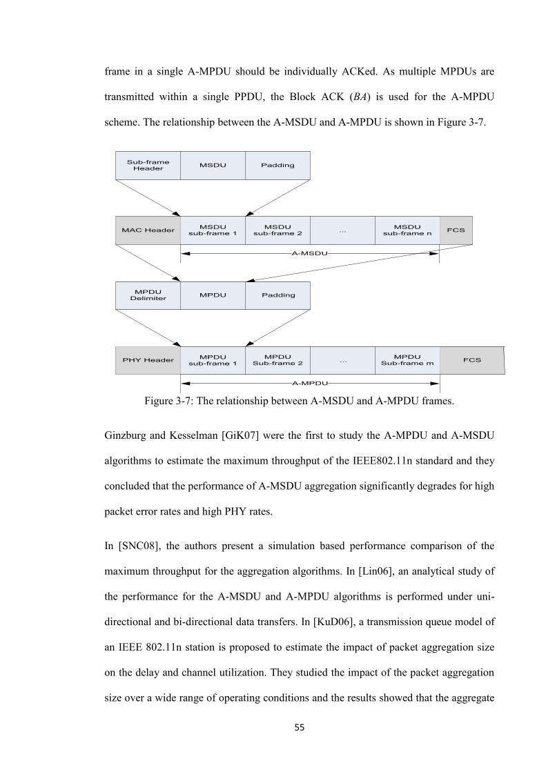
55
frame in a single A-MPDU should be individually ACKed. As multiple MPDUs are
transmitted within a single PPDU, the Block ACK (BA) is used for the A-MPDU
scheme. The relationship between the A-MSDU and A-MPDU is shown in Figure 3-7.
Sub-frame
HeaderMSDU Padding
MAC HeaderMSDU
sub-frame 1
MSDU
sub-frame 2...
MSDU
sub-frame nFCS
MPDU
DelimiterMPDU Padding
PHY HeaderMPDU
sub-frame 1
MPDU
Sub-frame 2...
MPDU
Sub-frame m
A-MSDU
A-MPDU
FCS
Figure 3-7: The relationship between A-MSDU and A-MPDU frames.
Ginzburg and Kesselman [GiK07] were the first to study the A-MPDU and A-MSDU
algorithms to estimate the maximum throughput of the IEEE802.11n standard and they
concluded that the performance of A-MSDU aggregation significantly degrades for high
packet error rates and high PHY rates.
In [SNC08], the authors present a simulation based performance comparison of the
maximum throughput for the aggregation algorithms. In [Lin06], an analytical study of
the performance for the A-MSDU and A-MPDU algorithms is performed under uni-
directional and bi-directional data transfers. In [KuD06], a transmission queue model of
an IEEE 802.11n station is proposed to estimate the impact of packet aggregation size
on the delay and channel utilization. They studied the impact of the packet aggregation
size over a wide range of operating conditions and the results showed that the aggregate
56
packet size is impacted by the packet arrival rate and data frame size. The authors in
[KHS08] propose an analytical model to evaluate the throughput performance based on
an enhanced discrete time Markov chain (DTMC). The results have shown that the
target aggregate packet size has little impact on the throughput in an unsaturated
network, while the throughput varies according to the target packet size in a saturated
network and the larger target aggregate packet size do not always yield better
throughput performance.
In [HLL08], an adaptive target aggregate packet size algorithm for A-MPDU in the
IEEE 802.11n networks is proposed to maximize the throughput by selecting the
optimal frame length under different channel conditions. The network throughput can
be further improved if it is employed together with the PHY rate adaption mechanism.
The performance of the algorithm with adaptive target aggregate packet size is better
than that of the algorithm with fixed target aggregate packet size. The idea of combining
fragmentation with A-MPDU aggregation is also presented in [SYC06] while the
authors in [SeS10] proposed a simple scheduling algorithm to determine which
aggregation option is used based on the packet size where the smallest size packet is
served first and this is referred to SSFS. However, in [SYC06], the authors ignore the
delay and just consider the reliability and throughput. It has the disadvantage that it
needs to change the format of MSDU which is not easy to implement.
In [SWS10], the authors compare the throughput performance of A-MSDU, A-MPDU
and PHY super-frames on different aggregation types and fragmentation types under
delay limits in an ultrahigh-speed WLAN. The authors in [SOS10] show that the header
size has a larger significant impact for the small sized MSDUs than that of large sized
MSDUs by using the packet aggregation algorithm. They present a packet aggregation
algorithm (mA-MSDU) which is described in [SOS11] to reduce the protocol overheads
57
and implement a re-transmission control over the individual sub-packets at the MSDU
level. The simulations results and analysis show a significant performance improvement
in terms of throughput for the proposed scheme particularly for applications that have a
small packet size such as VoIP.
[AbA11] shows the impact of the multi-rate operation on the A-MSDU and A-MPDU
based on the experiments using certified IEEE 802.11n equipment. Within A-MSDU
operation, an A-MSDU enabled station that operates at low data rate affects the
performance of A-MSDU disabled stations transmitting at higher rates. However,
within A-MPDU operation, the effect of not enabling A-MPDU for all stations is even
worse than the effect of multi-rate operation.
In [KML11], an adaptive aggregation scheme is proposed in order to resolve the
potential problem in A-MPDU where the sender transmits A-MSDUs within A-MPDUs
in an adaptive manner. A new analytical model to evaluate the performance of A-
MSDU and A-MPDU aggregation schemes is defined in [DAM11] where the model is
defined for a reliable multicast transport and allows the estimation of the MAC layer
efficiency. The proposed algorithm can improve the throughput over A-MSDU by up to
19% in the single hop network topology but it has poor performance in a multiple hop
network.
There are also some researchers who have studied some special applications (e.g. video)
for the A-MSDU and A-MPDU algorithms. The authors in [BaA12] study the
performance of packet aggregation to improve the efficiency and quality of the video
transmissions over the IEEE 802.11n wireless networks. In [ZCY10], they study the
impact of the video transmission for the packet aggregation, especially for the A-MPDU
algorithm in IEEE 802.11n wireless networks. It was found that when the optimal
58
packet aggregation size was changed following the channel conditions the throughput
was improved but this had little effect on the video quality.
For the technique described in [SeS10] may drop the packets in the queue as the packet
waits too long. This disadvantage is similar to [MBR12] where a real time scheduler
scheme is proposed which relies on traffic priority in order to support time sensitive
applications and satisfy the QoS requirements by employing A-MSDU. A scheme is
proposed in [KSP12] to determine the optimal frame size for the next transmission
using current channel information. In [KSP12], the authors employ frame size
estimation (FSE) with extended Kalman Filter (EKF) which uses a tight frame error rate
(FER) bound for OFDM system to obtain the instantaneous link quality. The
researchers found that the number of video streams that can be supported on the IEEE
802.11n networks depends on the implementation of the packet aggregation in [LYK08].
3.4.1 Discussion of A-MSDU and A-MPDU Schemes
A-MSDU and A-MPDU are the most popular packet aggregation algorithms which are
defined in the IEEE 802.11n standard and employed by the IEEE 802.11ac standard
draft to achieve the goal of high-throughput. The algorithm of A-MSDU combines
several MSDU packets into a large packet with a single MAC header and the A-MPDU
algorithm aggregates multiple MPDU packets into a large frame with a single PHY
header. Research studies on these two methods can be divided into two categories:
comparison of the performance for the two algorithms and determining the optimal
packet aggregation size and selection schemes to aggregate the packets.
Generally speaking, under a high BER environment, the A-MPDU algorithm is more
efficient in terms of throughput than that of the A-MSDU algorithm as only the
corrupted sub-packet needs to be re-transmitted in the A-MPDU algorithm while the
whole aggregate packet has to be re-transmitted in the A-MSDU algorithm if an error

59
occurs. Until now, a significant number of the proposed packet aggregation algorithms
based on the A-MSDU and A-MPDU algorithms try to determine the optimal target
aggregate packet size in different environments. Some proposed algorithms have good
performance in terms of throughput [KML11] [MBR12], however, they are not based
on the real live traffic loads. In this thesis, the A-MSDU algorithm is the typical FIFO
algorithm that is employed as the benchmark algorithm to be compared with the
proposed AAM algorithm. The other comparison algorithm used is the SSFS algorithm
[SeS10].
3.5 Chapter Summary
In this chapter, we have reviewed a number of different packet aggregation algorithms
which have been proposed by other researchers. As an upper limit on throughput and a
lower limit on delay exist in wireless networks, packet aggregation needs to be used to
improve the throughput. There exists a trade-off between the maximizing throughout
and minimizing delay. However, most of these researches were focused either on the
improvement in throughput or the reduction in delay. A number of different categories
of packet aggregation algorithms have been presented and the effect of the packet
aggregation algorithm on throughput and delay performances was studied in IEEE
802.11 WLANs. Some algorithms were presented that attempt to reduce the delay
increase to asymptotically approach the lower limit delay. The proposed packet
aggregation algorithms were divided into 4 categories: FF, FNF, AF and ANF. Two
most important packet aggregation algorithms, A-MSDU and A-MPDU, were
introduced which are defined in the IEEE 802.11n and IEEE 802.11ac standards. Many
studies of the two algorithms have been carried out.
60
Chapter 4 Proposed Packet Aggregation Algorithm
In chapter 2 and chapter 3, we discussed the background and the performance of the
packet aggregation algorithms proposed by other researchers. The most important
performance metrics for the packet aggregation algorithms are the throughput and the
delay. As described in the chapter 3, most of the proposed packet aggregation
algorithms attempt to optimize a single metric, i.e. either to maximize throughput or
minimize delay. These packet aggregation algorithms don’t take account of the varying
nature of the traffic load particularly the random nature of the packet size and packet
rate. For example, in [ZhN08] [SWC99], [BMS09], the authors focus on the optimal
aggregate packet size to achieve the maximum throughput but they don’t consider the
delay, while in [WeL11] and [LeP07] they just consider how to achieve the minimum
delay.
In this chapter we will outline the proposed packet aggregation algorithm called
Adaptive Aggregation Mechanism (AAM) which has been designed to achieve the goal
of the best aggregation trade-off in terms of realizing the maximum average throughput
with the minimum average delay compared to a number of popular aggregation
algorithms for different traffic loads in wireless network environments. The AAM
algorithm is an adaptive algorithm in that it responds to the varying nature of the packet
size and packet rate and attempts to assemble the target size aggregate packet with the
minimum delay.
In Figure 4-1, the structure of the AAM algorithm is shown. As can be seen, the AAM
algorithm is essentially a feedback control system which comprises three elements. The
first of these is the Adjustable Aggregation Algorithm (A3) which aggregates the
packets that are selected from a selection window in the input buffer. The selection
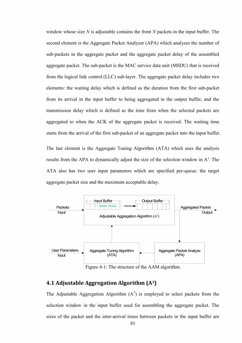
61
window whose size N is adjustable contains the front N packets in the input buffer. The
second element is the Aggregate Packet Analyzer (APA) which analyzes the number of
sub-packets in the aggregate packet and the aggregate packet delay of the assembled
aggregate packet. The sub-packet is the MAC service data unit (MSDU) that is received
from the logical link control (LLC) sub-layer. The aggregate packet delay includes two
elements: the waiting delay which is defined as the duration from the first sub-packet
from its arrival in the input buffer to being aggregated in the output buffer, and the
transmission delay which is defined as the time from when the selected packets are
aggregated to when the ACK of the aggregate packet is received. The waiting time
starts from the arrival of the first sub-packet of an aggregate packet into the input buffer.
The last element is the Aggregate Tuning Algorithm (ATA) which uses the analysis
results from the APA to dynamically adjust the size of the selection window in A3. The
ATA also has two user input parameters which are specified per-queue: the target
aggregate packet size and the maximum acceptable delay.
Adjustable Aggregation Algorithm (A3)
Aggregate Packet Analyze (APA)
Aggregate Tuning Algorithm (ATA)
Packets
Input
Aggregated Packet
Output
User Parameters
Input
Output BufferInput Buffer
Selection Window Selection
Figure 4-1: The structure of the AAM algorithm.
4.1 Adjustable Aggregation Algorithm (A3)
The Adjustable Aggregation Algorithm (A3) is employed to select packets from the
selection window in the input buffer used for assembling the aggregate packet. The
sizes of the packet and the inter-arrival times between packets in the input buffer are
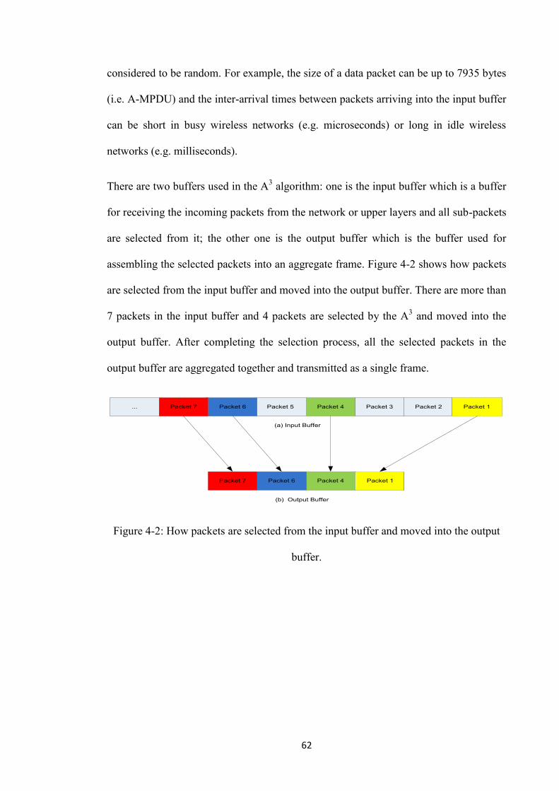
62
considered to be random. For example, the size of a data packet can be up to 7935 bytes
(i.e. A-MPDU) and the inter-arrival times between packets arriving into the input buffer
can be short in busy wireless networks (e.g. microseconds) or long in idle wireless
networks (e.g. milliseconds).
There are two buffers used in the A3 algorithm: one is the input buffer which is a buffer
for receiving the incoming packets from the network or upper layers and all sub-packets
are selected from it; the other one is the output buffer which is the buffer used for
assembling the selected packets into an aggregate frame. Figure 4-2 shows how packets
are selected from the input buffer and moved into the output buffer. There are more than
7 packets in the input buffer and 4 packets are selected by the A3 and moved into the
output buffer. After completing the selection process, all the selected packets in the
output buffer are aggregated together and transmitted as a single frame.
Packet 1Packet 2Packet 3Packet 4Packet 5...Packet 6Packet 7...
Packet 1Packet 4Packet 6
(a) Input Buffer
(b) Output Buffer
Packet 7
Figure 4-2: How packets are selected from the input buffer and moved into the output
buffer.
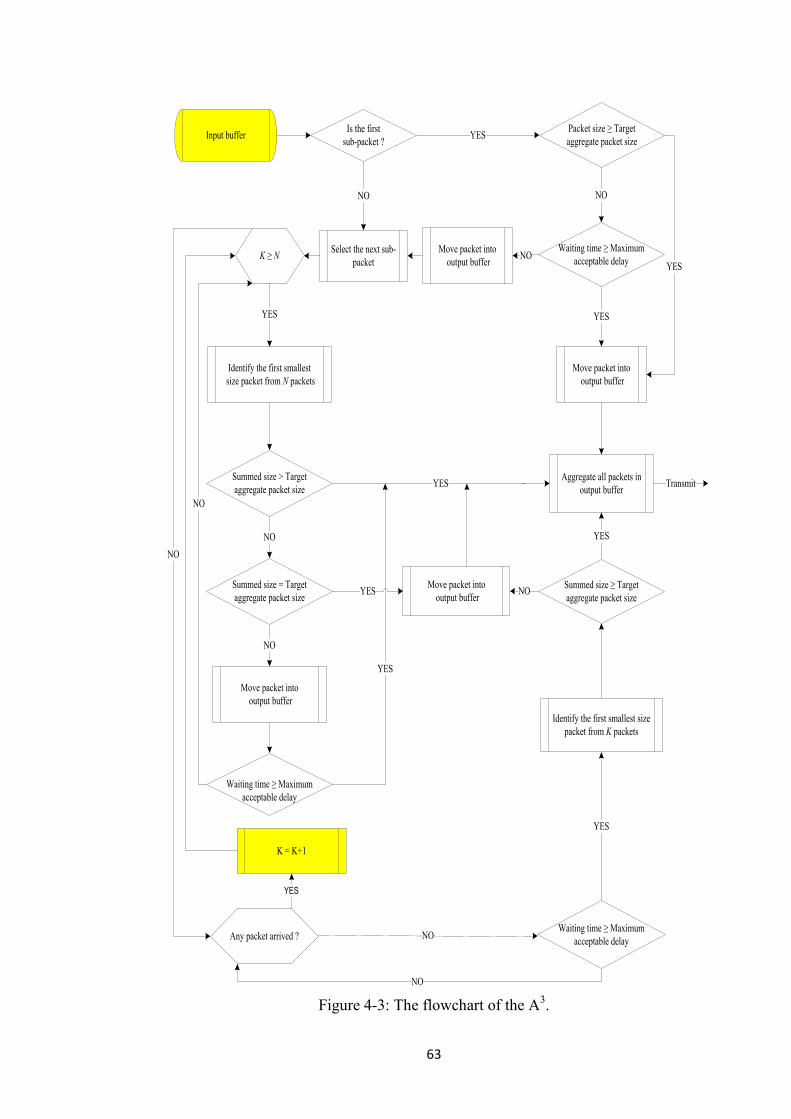
63
Input buffer
Move packet into
output buffer
Aggregate all packets in
output buffer
Waiting time ≥ Maximum
acceptable delay
Waiting time ≥ Maximum
acceptable delayNO
NO
Identify the first smallest size
packet from K packets
YES
Summed size ≥ Target
aggregate packet size
Move packet into
output buffer
Summed size = Target
aggregate packet size
Packet size ≥ Target
aggregate packet size YES
Move packet into
output buffer
Waiting time ≥ Maximum
acceptable delay
NO
Select the next sub-
packet
Identify the first smallest
size packet from N packets
Summed size > Target
aggregate packet size
YES
YES
NO
YES
NO
YES
NO
YES
NO
YES
Transmit
NO
K ≥ N
NO
Is the first
sub-packet ?
Any packet arrived ?
Move packet into
output buffer
YES
NO
K = K+1
YES
Figure 4-3: The flowchart of the A3.

64
The flowchart of A3 is shown in Figure 4-3. The size, N, is first initialised. Next, the
front packet in the input buffer is selected as the first sub-packet and its size is
compared with the target aggregate packet size.
(1) The packet is moved into the output buffer and transmitted if its size is greater
than or equal to the target aggregate packet size.
(2) If the packet size is smaller than the target aggregate packet size, the packet
waiting time in the input buffer is compared with the maximum acceptable
delay.
(3) If the waiting time is greater than or equal to the maximum acceptable delay,
the packet is moved into the output buffer and transmitted as soon as possible
without waiting for other packets to arrive.
(4) If the waiting time is less than the maximum acceptable delay, the packet is
moved into the output buffer and the algorithm selects the next sub-packet.
Assuming that the number of packets in the input buffer is K and the selection window
size is N, there are two outcomes that result from a comparison of K and N.
When K ≥ N, there are sufficient packets available for selection in the selection
window. At first, the first smallest size packet in the selection window is identified
where the first smallest size packet is the minimum length packet or the first one to have
arrived if more than one packet has the same minimum length in the selection window.
A3 compares the sum of this packet size and the selected packets sizes (i.e. the summed
size) with the target aggregate packet size.

65
(i) If the summed size is greater than the target aggregate packet size, the first
smallest size packet is not selected and all the selected packets in the output
buffer are aggregated together and transmitted as soon as possible.
(ii) If the summed size equals the target aggregate packet size, the first smallest size
packet is selected and moved into the output buffer to be aggregated with other
selected packets. Then the aggregate packet is transmitted as soon as possible.
(iii) If the summed size is less than the target aggregate packet size, the first smallest
size packet is selected and moved into the output buffer. Then the algorithm
checks the waiting time of the first sub-packet in the output buffer.
(iv) If it exceeds the maximum acceptable delay, all the selected packets in the
output buffer are aggregated into a single packet to be transmitted.
(v) Otherwise, the A3 resumes the process of selecting another sub-packet.
When K < N, there are insufficient packets to be selected from the selection window in
the input buffer and the algorithm must wait for packets to arrive. The maximum time to
wait is determined by the waiting time of the first sub-packet and the specified
maximum acceptable delay. During this time, if there are further packet arrivals into the
input buffer, the algorithm checks whether the inequality K < N applies or not.
(a) The case where K ≥ N has been described above.
(b) If K < N applies, then the A3 waits until the waiting time of first sub-packet
exceeds the maximum acceptable delay or K ≥ N applies.
(c) If the waiting time of first sub-packet exceeds the maximum acceptable delay
and K < N still applies, the first smallest size packet is selected from the K
packets. Then the algorithm processes the packet according to steps (i), (ii) and
(iii) described above until the summed size reaches the target aggregate packet
size or all K packets are selected. However, in step (iii) the algorithm does not

66
wait for more sub-packets and all the selected packets are aggregated and
transmitted as soon as possible.
The first sub-packet in every aggregate packet is always the front packet in the input
buffer. This rule ensures that the waiting time of the first sub-packet does not increase
indefinitely which can happen if the front packet were to be the biggest size packet in
the selection window.
In this scheme, the sub-packets may need to be reordered in the receiver. Based on the
IEEE 802.11n standard, the receiver contains a reordering buffer which is responsible
for reordering packets, so that the packets are eventually passed up to the next MAC
process in the order of received sequence number [IEn09]. The reordering process may
increase the delay as a packet may need to wait for other packets to arrive.
4.2 Aggregate Packet Analyzer (APA)
The aggregate packet analyzer (APA) is used to analyze the number of sub-packets and
the aggregate packet delay of the aggregate packet in order to determine the selection
window size for the next aggregate packet.
The APA analyses the current aggregate packet and the previous aggregate packet in
order to determine the value of N for the next aggregate packet where two registers are
used. Each register has two members, one is a counter used to record the number of sub-
packets and the other one is a timer used to record the aggregate packet delay. The value
of the counter of the number of sub-packets is incremented by 1 when a packet is
moved into the output buffer. When the first sub-packet is moved into the output buffer,
the waiting time of this packet in the input buffer is set as the value of the aggregate
packet delay timer and then it is incremented until the ACK for the aggregate packet is
received or the life time of the aggregate packet has been exceeded. The selection

67
process is stopped when the waiting time of the first sub-packet exceeds the maximum
acceptable delay or the summed size is greater than or equal to the target aggregate
packet size. The timer of the aggregate packet delay is frozen when an ACK for the
aggregate packet is received which also means the aggregate packet delay can be
determined. Each register counter and timer will be reset when the ACK for the
aggregate packet is received.
After an ACK frame is received, the APA algorithm calculates the differences in the
number of sub-packets and the aggregate packet delay between the current aggregate
packet and the previous aggregate packet. The outcomes are used to determine the
selection window size N in the ATA algorithm.
4.3 Aggregate Tuning Algorithm (ATA)
The third element of the AAM algorithm is the aggregate tuning algorithm (ATA)
which uses the analysis results from the APA to dynamically adjust the selection
window size N. The basic idea in developing the tuning rules is that the selection
window size is increased in order to improve the throughput when the network
performance is improved, while the selection window size is decreased in order to
reduce the delay when the network performance deteriorates. The analysis results from
the APA are used in ATA to determine the performance of network. The analysis results
are the change in the number of sub-packets and the change in the aggregate packet
delay, both of which are calculated between the current and the previous aggregate
packets. There are three outcomes for the change in the number of sub-packets: increase,
decrease and unchanged, and two outcomes for the change in the aggregate packet delay:
decrease and no decrease. Generally, a decrease in the aggregate packet delay means
that the performance of network is improving while an increase in the aggregate packet
delay means that the performance of network is getting worse.
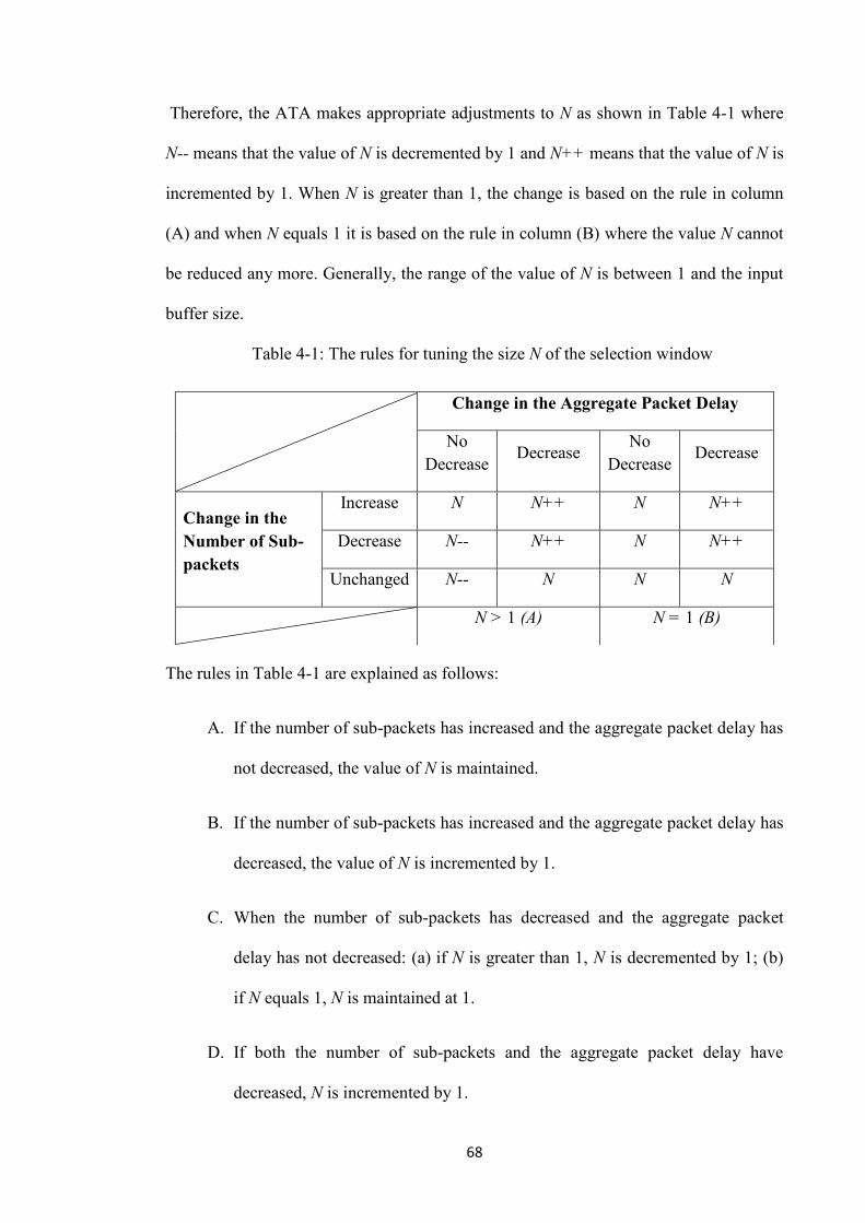
68
Therefore, the ATA makes appropriate adjustments to N as shown in Table 4-1 where
N-- means that the value of N is decremented by 1 and N++ means that the value of N is
incremented by 1. When N is greater than 1, the change is based on the rule in column
(A) and when N equals 1 it is based on the rule in column (B) where the value N cannot
be reduced any more. Generally, the range of the value of N is between 1 and the input
buffer size.
Table 4-1: The rules for tuning the size N of the selection window
The rules in Table 4-1 are explained as follows:
A. If the number of sub-packets has increased and the aggregate packet delay has
not decreased, the value of N is maintained.
B. If the number of sub-packets has increased and the aggregate packet delay has
decreased, the value of N is incremented by 1.
C. When the number of sub-packets has decreased and the aggregate packet
delay has not decreased: (a) if N is greater than 1, N is decremented by 1; (b)
if N equals 1, N is maintained at 1.
D. If both the number of sub-packets and the aggregate packet delay have
decreased, N is incremented by 1.
Change in the Aggregate Packet Delay
No
Decrease Decrease
No
Decrease Decrease
Change in the
Number of Sub-
packets
Increase N N++ N N++
Decrease N-- N++ N N++
Unchanged N-- N N N
N > 1 (A) N = 1 (B)
69
E. When the number of sub-packets is maintained and the aggregate packet delay
has not decreased: (a) if N is greater than 1, N is decremented by 1; (b) if N
equals 1, N is maintained at 1.
F. If the number of sub-packets is maintained and the aggregate packet delay has
decreased, N is maintained.
Increasing N increases the probability of achieving the target size of the aggregate
packet, but at the expense of a delay increase. Conversely, decreasing N reduces the
delay, but also may reduce the probability of achieving the target size of the aggregate
packet.
4.4 User Specified Input Parameters
In the AAM algorithm, the target aggregate packet size and the maximum acceptable
delay are specified by the user. The target aggregate packet size is the maximum size of
the aggregate packet and the maximum acceptable delay is the maximum time that the
A3 is allowed to wait in order to achieve the target aggregate packet size. The values of
these parameters are determined by the application being used. For example, if the user
wants to use a VoIP application (e.g. skype), the value of maximum acceptable delay is
set to 150 ms or less and the maximum acceptable delay could be set to 1 second when
the user wishes to use an email application. If the user wants to use both of them at the
same time, the maximum acceptable delay could be set to some appropriate value by the
user. Both of these user specified parameters, the target aggregate packet size and the
maximum acceptable delay, are the threshold values used to control the aggregation
process. The two parameters are set in the ATA and the values are sent to the A3 with
the selection window size N.

70
4.5 Analysis of All Three Aggregation Algorithms
In this thesis, the AAM algorithm is compared to two other packet aggregation
algorithms, FIFO and SSFS. The FIFO algorithm is used as the benchmark algorithm
which employs the most basic and popular packet selection strategy where all packets
are aggregated based on the packet arrival time and a selection window scheme is not
employed. The flow chart of the FIFO is shown in Figure 4-4. The A-MSDU algorithm
[IEn09] is employed as the typical FIFO algorithm to compare with the AAM algorithm.
The other algorithm is the SSFS algorithm (Smallest-Size First-Served) where all
packets are aggregated based on their size and a selection window scheme is also not
employed. The goal of the SSFS algorithm is to achieve the maximum number of sub-
packets in an aggregate packet [SeS10] associated with a large delay as it always tries to
wait for the smallest size packet to arrive. The flow chart of the SSFS is shown in
Figure 4-5. The AAM algorithm employs a selection window scheme and a hybrid
selection strategy which combines the FIFO and SSFS selection strategies where the
first sub-packet uses the FIFO selection strategy and the other sub-packets use the SSFS
selection strategy. The FIFO selection strategy ensures that the delay does not increase
indefinitely, while the SSFS selection strategy ensures that the maximum number of
sub-packets in an aggregate packet is achieved. The net result of this hybrid approach is
that the AAM algorithm can achieve the largest average aggregate packet size for all
three algorithms considered.
The throughput improvement is dependent upon the number of packets combined into
an aggregate packet in unit time compared to the non-aggregation case. In general, the
larger the number of packets that are assembled in unit time, the greater the throughput
improvement. As discussed in section 4.2, the aggregate packet delay includes two
elements, the waiting delay and the transmission delay. When the packet rate is high (i.e.

71
the inter-arrival time is small), the packet aggregation does not require extra time for
packets to arrive compared to non-aggregation [ZIF08]. Therefore, the aggregate packet
delay is dependent upon the transmission delay which is dependent on the PHY rate and
the aggregate packet size based on the equation (3.2) [XiR02]. With a fixed PHY rate,
the aggregate packet delay is dependent on the aggregate packet size for small values of
the inter-arrival time. The reason is that generally a larger average size of the aggregate
packet corresponds to a larger average number of sub-packets per aggregate packet
which can reduce some of the delays associated with each transmission such as the
access medium time (e.g. DIFS) for the sub-packet and the transmission time of the
MAC header and ACK.
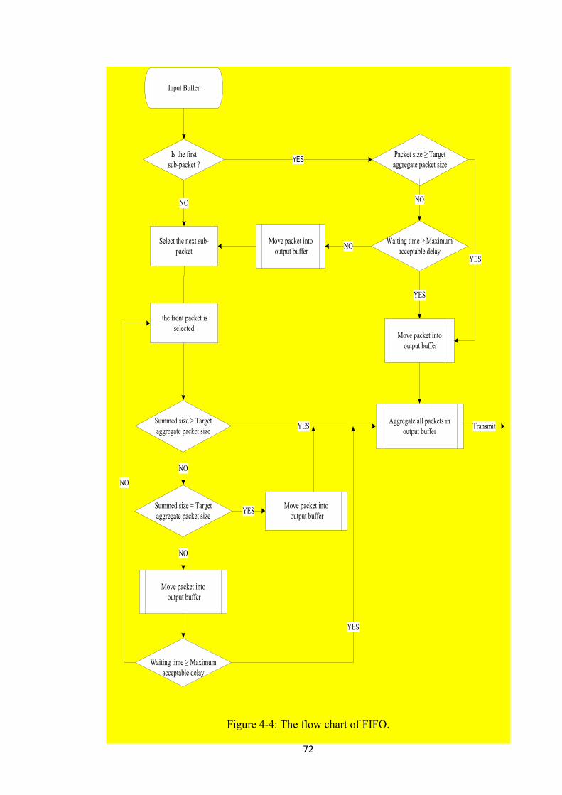
72
Input Buffer
Move packet into
output buffer
Aggregate all packets in
output buffer
Waiting time ≥ Maximum
acceptable delay
Move packet into
output buffer
Summed size = Target
aggregate packet size
Packet size ≥ Target
aggregate packet size
Move packet into
output buffer
Waiting time ≥ Maximum
acceptable delay
NO
the front packet is
selected
Summed size > Target
aggregate packet size YES
NO
YES
NO
YES
NO
YES
Transmit
NO
Is the first
sub-packet ?
Move packet into
output buffer
YES
NOSelect the next sub-
packet
YES
Figure 4-4: The flow chart of FIFO.

73
Input Buffer
Aggregate all packets in
output buffer
Packet size ≥ Target
aggregate packet size
YES
Move packet into
output buffer
Is the input buffer
full ?
NO
Waiting time ≥ Maximum
acceptable delay
Identify the first
smallest size packet
YES
NO
Move packet into
output bufferNO
Transmit
YES
Figure 4-5: The flow chart of SSFS.
In this section, we will discuss the interactions between the different parameters for the
three packet aggregation algorithms. Figure 4-6 shows the interaction between the
different parameters of the FIFO algorithm which is an example of an open control
system. The positive sign is used to indicate that if the inter-arrival time increases this
causes an increase in waiting delay because the FIFO algorithm aggregates the packets
based on the packet arrival time. The negative sign is used to indicate that if the arrival
packet size decreases this causes an increase in the number of sub-packets per aggregate
packet because it requires a combining of more packets into an aggregate packet in
order to reach the target aggregate packet size. This can be explained as follows: if the
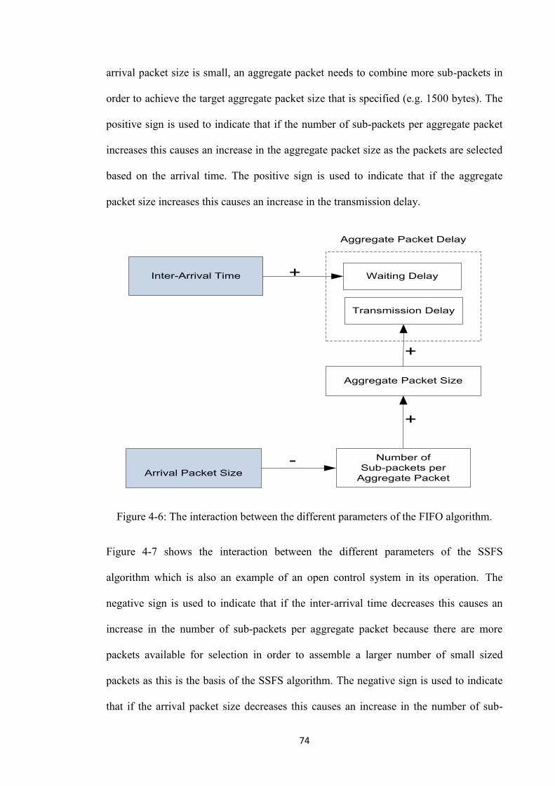
74
arrival packet size is small, an aggregate packet needs to combine more sub-packets in
order to achieve the target aggregate packet size that is specified (e.g. 1500 bytes). The
positive sign is used to indicate that if the number of sub-packets per aggregate packet
increases this causes an increase in the aggregate packet size as the packets are selected
based on the arrival time. The positive sign is used to indicate that if the aggregate
packet size increases this causes an increase in the transmission delay.
Inter-Arrival Time +
Arrival Packet Size
- Number of
Sub-packets per
Aggregate Packet
Aggregate Packet Size
+
+
Waiting Delay
Transmission Delay
Aggregate Packet Delay
Figure 4-6: The interaction between the different parameters of the FIFO algorithm.
Figure 4-7 shows the interaction between the different parameters of the SSFS
algorithm which is also an example of an open control system in its operation. The
negative sign is used to indicate that if the inter-arrival time decreases this causes an
increase in the number of sub-packets per aggregate packet because there are more
packets available for selection in order to assemble a larger number of small sized
packets as this is the basis of the SSFS algorithm. The negative sign is used to indicate
that if the arrival packet size decreases this causes an increase in the number of sub-

75
packets per aggregate packet as it requires assembling more packets to reach the target
aggregate packet size.
Number
of Sub-packets per
Aggregate Packet
-Inter-Arrival Time
Arrival Packet Size
-
Figure 4-7: The interaction between the different parameters of the SSFS algorithm.
Inter-Arrival Time
Number of
Sub-packets per
Aggregate Packet
Aggregate
Packet Size
Selection Window
Size
-+
-
+ Arrival Packet Size+
Waiting Delay
Transmission Delay
Aggregate Packet Delay
-
+
Figure 4-8: The interaction between the different parameters of the AAM algorithm.
Figure 4-8 presents the interaction between the different parameters of the AAM
algorithm which is an example of a feedback control system. The negative sign is used
to indicate that if the inter-arrival time decreases this causes an increase in the number
of sub-packets per aggregate packet where the explanation is the same as that for the
SSFS algorithm. The positive sign is used to indicate that if the inter-arrival time
increases this causes an increase in waiting delay because the first sub-packet is selected
based on the arrival time. The negative sign is used to indicate that if the arrival packet

76
size decreases this causes an increase in the number of sub-packets per aggregate packet
where the explanation is the same as that for the SSFS algorithm. The positive sign is
used to indicate that if the number of sub-packets per aggregate packet increases this
causes an increase in the aggregate packet size where the explanation is the same as that
for the FIFO algorithm. The positive sign is used to indicate that if the aggregate packet
size increases this causes an increase in the transmission delay. The negative sign is
used to indicate that if the aggregate packet delay decreases this causes an increase in
the selection window size according to the tuning rules shown in Table 4-1. The
positive sign is used to indicate that if the selection window size increases this causes an
increase in the probability of achieving a larger number of sub-packets per aggregate
packet.
In Figure 4-8, there is a negative feedback loop formed between the number of sub-
packets per aggregate packet, aggregate packet size, aggregate packet delay and
selection window size when raw packets can be aggregated (i.e. when packet
aggregation can occur). Increasing the number of sub-packets per aggregate packet
leads to an increase in the aggregate packet size and an increase in the aggregate packet
size increases the aggregate packet delay as the transmission delay increases. An
increase in the aggregate packet delay decreases the selection window size according to
the tuning rules shown in Table 4-1 and a decrease in the selection window size
decreases the probability of achieving a larger number of sub-packets per aggregate
packet.
Based on the previous discussion, the AAM algorithm is a feedback control system and
can operate with random packet size and packet rate. The AAM algorithm has a better
performance compared to the other two algorithms (i.e. FIFO and SSFS) as will be
demonstrated by the results presented in chapter 5.
77
4.6 Simulation
In this thesis, the AAM algorithm is implemented in two scenarios. In the first scenario,
the aggregation process of the AAM algorithm is implemented as a standalone C++
computer program. In this test scenario, there are two objectives: (i) To demonstrate that
the AAM algorithm is an adaptive algorithm that can operate over a wide range of
different traffic loads; (ii) To demonstrate that the AAM algorithm has a superior
performance compared to that of the FIFO and SSFS algorithms in terms of the number
of sub-packets per aggregate packet for a given delay (i.e. waiting delay) by employing
a selection window scheme associated with the hybrid selection strategy. In the second
test scenario, the AAM algorithm is implemented in a wireless network containing an
AP and a client station. This test scenario has been implemented in the ns-3 simulator.
The objectives of the second scenario is to demonstrate that the AAM algorithm (i) has
a superior performance compared to the other two algorithms in terms of the
aggregation trade-off in achieving the maximum average throughput with the minimum
average delay in wireless networks; and (ii) can significantly improve the performance
in terms of the average throughput in error-prone wireless networks.
In the two test scenarios, 16 captured traffic trace files are used as the input. All of these
traffic trace files were captured from live Wi-Fi hotspot networks by using the network
sniffer tool wireshark. These traffic trace files were captured at different locations, such
as in a library, university campus, coffee shop, train station and airport, and were also
captured at different times from 29th
May 2012 to 17th
July 2012. The details of the 16
captured traffic trace files are shown in Table 4-2.
There are two parameters selected as input to the simulation namely the packet size and
the packet arrival time. The advantages of using this approach to generate the network
test traffic profiles are the following: Firstly, these captured traffic trace files better

78
represent the typical traffic patterns found on data networks. Secondly, these captured
traffic trace files represent the characteristics of a traffic load containing different types
of application. These captured traffic trace files differ from each other in terms of the
packet size and the inter-arrival time between packets.
Table 4-2: The details of the 16 captured traffic trace files
ID Capture Date Capture
Time
Number of
captured
Packets
Average
Packet Size
(bytes)
Average
Packet
Rate (pps)
Capture Location
1 29th May 2012 10:30—11:30 331649 552 92.1 JAVA City, DIT, Dublin
2 29th May 2012 12:00—13:00 410444 576 114.0 JAVA City, DIT, Dublin
3 29th May 2012 14:00—15:00 272349 550 75.7 JAVA City, DIT, Dublin
4 29th May 2012 16:00—17:00 400514 588 111.3 JAVA City, DIT, Dublin
5 29th May 2012 17:30—19:30 393944 590 109.4 JAVA City, DIT, Dublin
6 19th June 2012 09:30—10:30 33958 442 9.4 Costa Coffee, Dawson St, Dublin
7 19th June 2012 11:00—12:00 20255 235 5.6 Parliament Square, TCD, Dublin
8 19th June 2012 12:30—13:30 33156 440 9.2 Costa Coffee, Dawson St, Dublin
9 19th June 2012 16:00—17:00 12998 223 3.6 Parliament Square, TCD, Dublin
10 19th June 2012 17:00—18:00 23933 571 6.6 Costa Coffee, Dawson St, Dublin
11 24th June 2012 12:00-13:00 24747 317 6.9 Hueston train station, Dublin
12 24th June 2012 13:30-14:30 15242 94 4.2 Hueston train station, Dublin
13 24th June 2012 15:00—16:00 22358 137 6.2 Hueston train station, Dublin
14 26th June 2012 10:30—11:30 69299 399 19.2 Library, Kevin Str., DIT, Dublin
15 26th June 2012 12:00—13:00 13785 155 3.8 Library, Kevin Str., DIT, Dublin
16 17th July 2012 19:00—19:50 24962 694 8.3
Shuangliu Airport, Chengdu,
China
Where JAVA City is a name of a popular student coffee shop on the campus of Dublin
Institute of Technology and TCD is Trinity College Dublin. As a lot of RTS/CTS
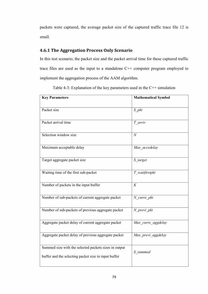
79
packets were captured, the average packet size of the captured traffic trace file 12 is
small.
4.6.1 The Aggregation Process Only Scenario
In this test scenario, the packet size and the packet arrival time for these captured traffic
trace files are used as the input to a standalone C++ computer program employed to
implement the aggregation process of the AAM algorithm.
Table 4-3: Explanation of the key parameters used in the C++ simulation
Key Parameters Mathematical Symbol
Packet size S_pkt
Packet arrival time T_arriv
Selection window size N
Maximum acceptable delay Max_accedelay
Target aggregate packet size S_target
Waiting time of the first sub-packet T_waitfirstpkt
Number of packets in the input buffer K
Number of sub-packets of current aggregate packet N_curre_pkt
Number of sub-packets of previous aggregate packet N_previ_pkt
Aggregate packet delay of current aggregate packet Max_curre_aggdelay
Aggregate packet delay of previous aggregate packet Max_previ_aggdelay
Summed size with the selected packets sizes in output
buffer and the selecting packet size in input buffer
S_summed
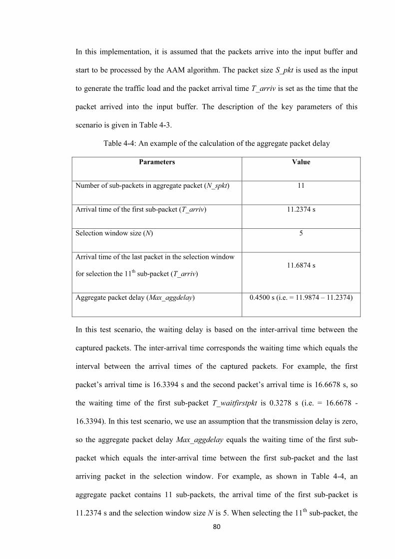
80
In this implementation, it is assumed that the packets arrive into the input buffer and
start to be processed by the AAM algorithm. The packet size S_pkt is used as the input
to generate the traffic load and the packet arrival time T_arriv is set as the time that the
packet arrived into the input buffer. The description of the key parameters of this
scenario is given in Table 4-3.
Table 4-4: An example of the calculation of the aggregate packet delay
Parameters Value
Number of sub-packets in aggregate packet (N_spkt) 11
Arrival time of the first sub-packet (T_arriv) 11.2374 s
Selection window size (N) 5
Arrival time of the last packet in the selection window
for selection the 11th sub-packet (T_arriv)
11.6874 s
Aggregate packet delay (Max_aggdelay) 0.4500 s (i.e. = 11.9874 – 11.2374)
In this test scenario, the waiting delay is based on the inter-arrival time between the
captured packets. The inter-arrival time corresponds the waiting time which equals the
interval between the arrival times of the captured packets. For example, the first
packet’s arrival time is 16.3394 s and the second packet’s arrival time is 16.6678 s, so
the waiting time of the first sub-packet T_waitfirstpkt is 0.3278 s (i.e. = 16.6678 -
16.3394). In this test scenario, we use an assumption that the transmission delay is zero,
so the aggregate packet delay Max_aggdelay equals the waiting time of the first sub-
packet which equals the inter-arrival time between the first sub-packet and the last
arriving packet in the selection window. For example, as shown in Table 4-4, an
aggregate packet contains 11 sub-packets, the arrival time of the first sub-packet is
11.2374 s and the selection window size N is 5. When selecting the 11th
sub-packet, the
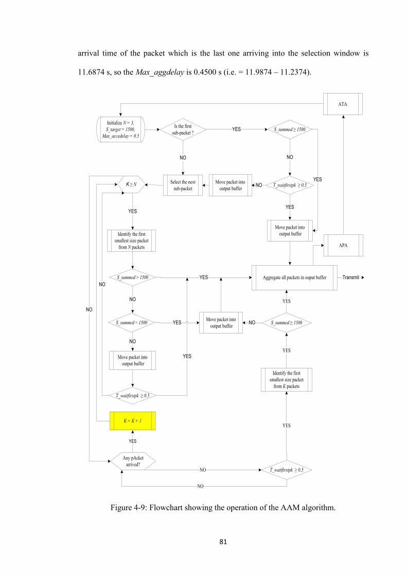
81
arrival time of the packet which is the last one arriving into the selection window is
11.6874 s, so the Max_aggdelay is 0.4500 s (i.e. = 11.9874 – 11.2374).
Initialize N = 3,
S_target = 1500,
Max_accedelay = 0.5
Move packet into
output buffer
Aggregate all packets in ouput buffer
T_waitfirstpk ≥ 0.5
T_waitfirstpk ≥ 0.5NO
NO
Identify the first
smallest size packet
from K packets
YES
S_summed ≥ 1500
YES
Move packet into
output bufferS_summed = 1500
S_summed ≥ 1500 YES
Move packet into
output buffer
T_waitfirstpk ≥ 0.5
NO
Select the next
sub-packet
Identify the first
smallest size packet
from N packets
S_summed > 1500
YES
YES
NO
YES
NO
YES
NO
YES
NO
Transmit
NO
K ≥ N
NO
Is the first
sub-packet ?
Any pAcket
arrived?
Move packet into
output buffer
YES
NO
APA
ATA
YES
K = K + 1
YES
Figure 4-9: Flowchart showing the operation of the AAM algorithm.
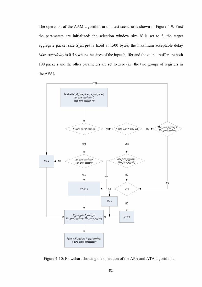
82
The operation of the AAM algorithm in this test scenario is shown in Figure 4-9. First
the parameters are initialized; the selection window size N is set to 3, the target
aggregate packet size S_target is fixed at 1500 bytes, the maximum acceptable delay
Max_accedelay is 0.5 s where the sizes of the input buffer and the output buffer are both
100 packets and the other parameters are set to zero (i.e. the two groups of registers in
the APA).
Initialize N =3, N_curre_pkt = 0, N_previ_pkt = 0,
Max_curre_aggdelay = 0,
Max_previ_aggdelay = 0
N_curre_pkt > N_previ_pkt
Max_curre_aggdelay <
Max_previ_aggdelay
YES
N = N + 1
YES
N = N NO
N_previ_pkt = N_curre_pkt
Max_previ_aggdelay = Max_curre_aggdelay
N_curre_pkt < N_previ_pktNO
Max_curre_aggdelay <
Max_previ_aggdelay
YES
YES
N = 1
NO
N = N
N = N-1
NO
YES
NOMax_curre_aggdelay <
Max_previ_aggdelay
YES
NO
Return N, N_previ_pkt, N_previ_aggdelay,
N_curre_pkt,N_curreaggdelay
Figure 4-10: Flowchart showing the operation of the APA and ATA algorithms.
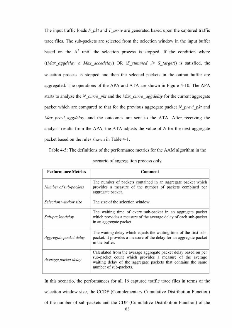
83
The input traffic loads S_pkt and T_arriv are generated based upon the captured traffic
trace files. The sub-packets are selected from the selection window in the input buffer
based on the A3 until the selection process is stopped. If the condition where
((Max_aggdelay ≥ Max_accedelay) OR (S_summed ≥ S_target)) is satisfied, the
selection process is stopped and then the selected packets in the output buffer are
aggregated. The operations of the APA and ATA are shown in Figure 4-10. The APA
starts to analyze the N_curre_pkt and the Max_curre_aggdelay for the current aggregate
packet which are compared to that for the previous aggregate packet N_previ_pkt and
Max_previ_aggdelay, and the outcomes are sent to the ATA. After receiving the
analysis results from the APA, the ATA adjusts the value of N for the next aggregate
packet based on the rules shown in Table 4-1.
Table 4-5: The definitions of the performance metrics for the AAM algorithm in the
scenario of aggregation process only
Performance Metrics Comment
Number of sub-packets
The number of packets contained in an aggregate packet which
provides a measure of the number of packets combined per
aggregate packet.
Selection window size The size of the selection window.
Sub-packet delay
The waiting time of every sub-packet in an aggregate packet
which provides a measure of the average delay of each sub-packet
in an aggregate packet.
Aggregate packet delay
The waiting delay which equals the waiting time of the first sub-
packet. It provides a measure of the delay for an aggregate packet
in the buffer.
Average packet delay
Calculated from the average aggregate packet delay based on per
sub-packet count which provides a measure of the average
waiting delay of the aggregate packets that contains the same
number of sub-packets.
In this scenario, the performances for all 16 captured traffic trace files in terms of the
selection window size, the CCDF (Complementary Cumulative Distribution Function)
of the number of sub-packets and the CDF (Cumulative Distribution Function) of the

84
sub-packet delay, the number of sub-packets against the average aggregate packet delay
for the AAM algorithm will be presented in chapter 5. The average packet delay is the
mean aggregate packet delay based on the per sub-packet count. This means that all
aggregate packets which have the same number of sub-packets are used to calculate the
average packet delay. For example, an average packet delay is calculated for all
aggregate packets containing 7 sub-packets aggregate packets and similarly for all
aggregate packets containing 8 sub-packets and so on. The parameters used to analyze
the performance of the AAM algorithm in this scenario are shown in Table 4-5.
4.6.2 Deployment Scenario in Wireless Networks
The second test scenario is implemented on the ns-3.14 simulation tool where the AAM
algorithm has been deployed in a wireless network. The AAM algorithm is
implemented in an IEEE 802.11 WLAN with and without transmission errors present,
and the payloads of the packets are based on the packet sizes found in the captured
traffic trace files.
Figure 4-11: The topology of the wireless network in the ns-3 simulation.
The topology used is shown in Figure 4-11. The wireless network contains two stations,
one station is the receiver station (i.e. with IP address 196.168.1.2) which is also the
access point (AP), and the other one is operated as the source station (i.e. with IP
address 196.168.1.1) which is also the client station. The distance between the stations
is 50 meters.
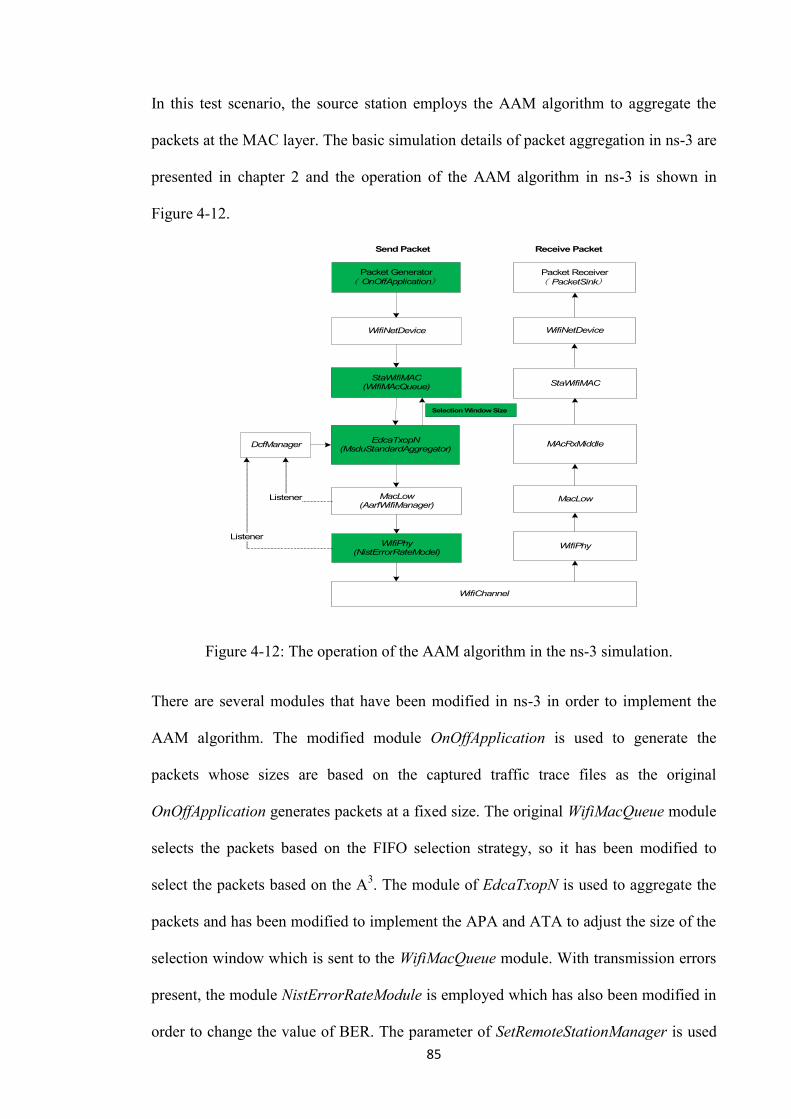
85
In this test scenario, the source station employs the AAM algorithm to aggregate the
packets at the MAC layer. The basic simulation details of packet aggregation in ns-3 are
presented in chapter 2 and the operation of the AAM algorithm in ns-3 is shown in
Figure 4-12.
Packet Generator
( OnOffApplication)
WifiNetDevice
StaWifiMAC (WifiMAcQueue)
EdcaTxopN(MsduStandardAggregator)
MacLow(AarfWifiManager)
WifiPhy(NistErrorRateModel)
WifiChannel
DcfManager
Listener
Listener
Packet Receiver
( PacketSink)
MAcRxMiddle
MacLow
WifiPhy
StaWifiMAC
Send Packet Receive Packet
WifiNetDevice
Selection Window Size
Figure 4-12: The operation of the AAM algorithm in the ns-3 simulation.
There are several modules that have been modified in ns-3 in order to implement the
AAM algorithm. The modified module OnOffApplication is used to generate the
packets whose sizes are based on the captured traffic trace files as the original
OnOffApplication generates packets at a fixed size. The original WifiMacQueue module
selects the packets based on the FIFO selection strategy, so it has been modified to
select the packets based on the A3. The module of EdcaTxopN is used to aggregate the
packets and has been modified to implement the APA and ATA to adjust the size of the
selection window which is sent to the WifiMacQueue module. With transmission errors
present, the module NistErrorRateModule is employed which has also been modified in
order to change the value of BER. The parameter of SetRemoteStationManager is used
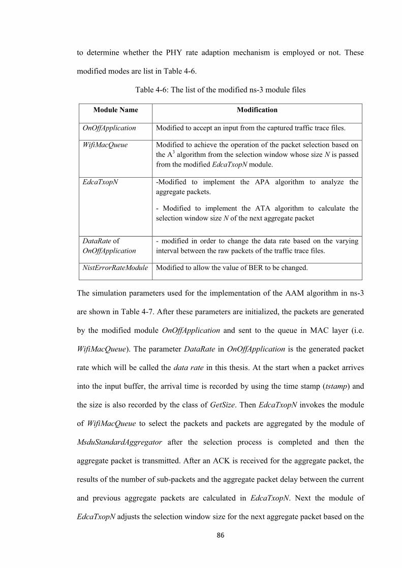
86
to determine whether the PHY rate adaption mechanism is employed or not. These
modified modes are list in Table 4-6.
Table 4-6: The list of the modified ns-3 module files
Module Name Modification
OnOffApplication Modified to accept an input from the captured traffic trace files.
WifiMacQueue Modified to achieve the operation of the packet selection based on
the A3 algorithm from the selection window whose size N is passed
from the modified EdcaTxopN module.
EdcaTxopN -Modified to implement the APA algorithm to analyze the
aggregate packets.
- Modified to implement the ATA algorithm to calculate the
selection window size N of the next aggregate packet
DataRate of
OnOffApplication
- modified in order to change the data rate based on the varying
interval between the raw packets of the traffic trace files.
NistErrorRateModule Modified to allow the value of BER to be changed.
The simulation parameters used for the implementation of the AAM algorithm in ns-3
are shown in Table 4-7. After these parameters are initialized, the packets are generated
by the modified module OnOffApplication and sent to the queue in MAC layer (i.e.
WifiMacQueue). The parameter DataRate in OnOffApplication is the generated packet
rate which will be called the data rate in this thesis. At the start when a packet arrives
into the input buffer, the arrival time is recorded by using the time stamp (tstamp) and
the size is also recorded by the class of GetSize. Then EdcaTxopN invokes the module
of WifiMacQueue to select the packets and packets are aggregated by the module of
MsduStandardAggregator after the selection process is completed and then the
aggregate packet is transmitted. After an ACK is received for the aggregate packet, the
results of the number of sub-packets and the aggregate packet delay between the current
and previous aggregate packets are calculated in EdcaTxopN. Next the module of
EdcaTxopN adjusts the selection window size for the next aggregate packet based on the

87
rules shown in Table 4-1 and then it sends the updated value of N to the module of
WifiMacQueue.
Table 4-7: The simulation parameters used to implement the AAM algorithm in ns-3
Parameter Value
Number of stations 2
Initial size of the selection window 3
Distance between stations (m) 50
Maxpacketnumber in WifiMacQueu 400
Max. acceptable delay in EdcaTxopN (second) 0.05
MaxSlrc in AarfWifiManager 10
MaxSuccessThreshold in AarfWifiManager 100
MaxAmsduSize in MsduStandardAggregator 1500
PHY rate adaption module AarfWifiManager
Transmission errors module NistErrorRateModule
PHY rate (Mbps) 6, 9, 12, 18, 24, 36, 48, 54
DataRate in OnOffApplication 2, 4, 6, 8, 10, 12, 14, 16,18, 20, 22, 24, 26,
28,30
BER in NistErrorRateModule
10-5
, 10-4
, 5×10⁻⁴
, 10-3
, 1.5×10⁻³
, 1.6×10⁻³
,
1.7×10⁻³
, 1.8×10⁻³
, 1.9×10⁻³
, 2×10⁻³
,
2.1×10⁻³
, 2.2×10⁻³
, 2.3×10⁻³
, 2.5×10⁻³
,
3×10⁻³
, 4×10⁻³
, 6×10⁻³
, 8×10⁻³
, 10-2
, 2×10⁻²
When the AAM algorithm is implemented in a wireless network without transmission
errors present and also without employing the PHY rate adaption mechanism, the PHY
rate can be set to 6 Mbps, 9 Mbps, 12 Mbps, 18 Mbps, 24 Mbps, 36 Mbps, 48 Mbps and
54 Mbps, which is implemented by the parameter SetRemoteStationManager set to
ConstantRateWifiManager, and the data rate is changed by controlling the parameter
DataRate in the OnOffApplication module. The transmission errors module

88
NistErrorRateModule and PHY rate adaption mechanism module AarfWifiManager are
not employed.
Table 4-8: The performance metrics for analysis the AAM algorithm in the deployment
scenario in wireless networks
Performance Metric Definition
Throughput The average payload in bits per second successfully
transmitted from the source node to the destination node.
Maximum average throughput The average throughput when the wireless network is
saturated.
Average delay
The average time required to successfully transmit packets
from the MAC layer of the source node to the MAC layer of
the destination node.
Minimum average delay The average delay when the wireless network is saturated.
Aggregation trade-off The maximum average throughput with the minimum average
delay in wireless networks.
Deviation Defined as the difference between the target aggregate
packet size and the aggregate packet size.
Mean square deviation The average value of the square of the deviation.
Data rate
The data rate (in bits per second) arriving into the buffer which
equals the generated data rate of the generator (i.e. DataRate in
OnOffApplication)
BER The Bit Error Rate used to characterize the transmission errors
In this test scenario, different values of BER are used (as shown in Table 4-7) in order
to demonstrate that the AAM algorithm is a robust algorithm. When the AAM
algorithm is implemented in the error-prone wireless networks the
NistErrorRateModule is modified to set the different values of the BER. The PHY rate
adaption module AarfWifiManager which is based on the adaptive auto rate fallback
(AARF) [LMT04] is employed to select the PHY rate, where the module
AarfWifiManager is invoked by the parameter SetRemoteStationManager.
89
The performance metrics used to analyze these performances for the AAM algorithm in
this scenario are shown in Table 4-8 and the results will be presented in chapter 5.
4.7 Chapter Summary
This chapter has presented the proposed packet aggregation algorithm AAM that is an
adaptive algorithm and is essentially a feedback control system which tries to achieve
the best aggregation trade-off in terms of realizing the maximum average throughput
with the minimum average delay for the different traffic loads typically found in real
wireless networks. To the best of our knowledge the AAM algorithm is the first packet
aggregation algorithm to employ a tunable selection window scheme for the selection of
sub-packets.
The AAM algorithm comprises three elements: Adjustable Aggregation Algorithm (A3),
Aggregate Packet Analyzer (APA) and Aggregate Tuning Algorithm (ATA). The
adjustable aggregation algorithm (A3) assembles the aggregate packet by selecting
packets from a selection window. The size of this selection window is adaptive.
Increasing the size of the selection window increases the probability of achieving the
target aggregate packet size of the aggregate packet at the expense of a delay increase.
Conversely, decreasing the size of the selection window reduces the delay, but also
reduces the probability of achieving the target aggregate packet size. The aggregate
packet analyzer (APA) analyzes the number of sub-packets in the aggregate packet and
the aggregate packet delay associated with assembling the aggregate packet. The
aggregate tuning algorithm (ATA) uses the analysis results from the APA to adaptively
adjust the size of the selection window. The ATA has two input parameters specified by
the user: the target aggregate packet size and the maximum acceptable delay which are
the threshold values used to control the aggregation process of the AAM algorithm. The

90
interaction between the different parameters for all three algorithms considered (i.e.
FIFO, SSFS and AAM) is discussed.
After an introduction and an analysis of the proposed AAM algorithm, the two test
scenarios which are employed to implement the AAM algorithm were described. The
first test scenario was used to demonstrate that the AAM algorithm is an adaptive
algorithm that has a superior performance in terms of the number of sub-packets per
aggregate packet for a given average packet delay. In this test scenario, a standalone
computer program was developed using C++ and 16 captured traffic trace files which
were captured from live Wi-Fi hotspot networks and were used to provide an input
traffic profile. In the second test scenario, the AAM algorithm was deployed in a
wireless network by using the ns-3 simulator. The AAM algorithm was implemented in
the source node to analyze the performances in terms of throughput, delay and
aggregation trade-off in achieving the maximum average throughput with the minimum
average delay in wireless networks with and without transmission errors present.
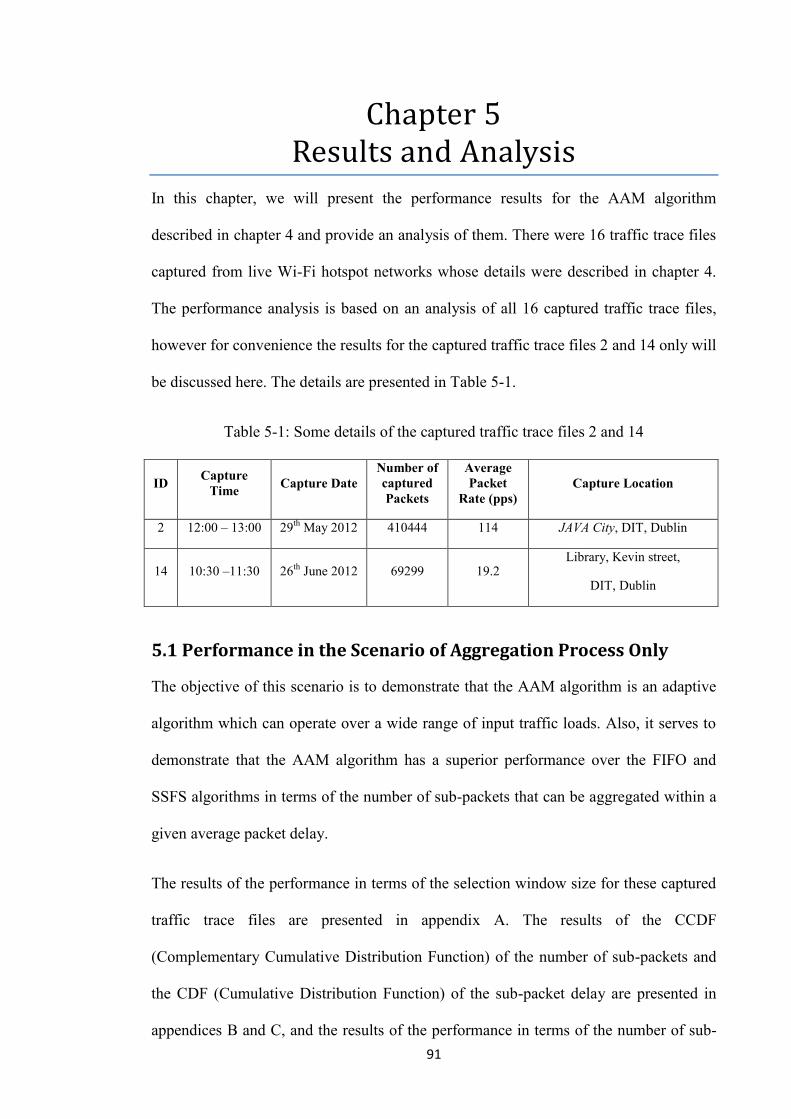
91
Chapter 5 Results and Analysis
In this chapter, we will present the performance results for the AAM algorithm
described in chapter 4 and provide an analysis of them. There were 16 traffic trace files
captured from live Wi-Fi hotspot networks whose details were described in chapter 4.
The performance analysis is based on an analysis of all 16 captured traffic trace files,
however for convenience the results for the captured traffic trace files 2 and 14 only will
be discussed here. The details are presented in Table 5-1.
Table 5-1: Some details of the captured traffic trace files 2 and 14
ID Capture
Time Capture Date
Number of
captured
Packets
Average
Packet
Rate (pps)
Capture Location
2 12:00 – 13:00 29th
May 2012 410444 114 JAVA City, DIT, Dublin
14 10:30 –11:30 26th
June 2012 69299 19.2 Library, Kevin street,
DIT, Dublin
5.1 Performance in the Scenario of Aggregation Process Only
The objective of this scenario is to demonstrate that the AAM algorithm is an adaptive
algorithm which can operate over a wide range of input traffic loads. Also, it serves to
demonstrate that the AAM algorithm has a superior performance over the FIFO and
SSFS algorithms in terms of the number of sub-packets that can be aggregated within a
given average packet delay.
The results of the performance in terms of the selection window size for these captured
traffic trace files are presented in appendix A. The results of the CCDF
(Complementary Cumulative Distribution Function) of the number of sub-packets and
the CDF (Cumulative Distribution Function) of the sub-packet delay are presented in
appendices B and C, and the results of the performance in terms of the number of sub-
92
packets against the average packet delay are presented in appendix D. The CCDF of the
number of sub-packets and the CDF of the sub-packet delay are used to analyze the
performance of the AAM algorithm. The CCDF and CDF allow us to make a
meaningful comparison of the performances for the different algorithms. The CCDF of
the number of sub-packets is the probability that the number of sub-packets takes on a
value greater than or equal to a certain value which allows us to compare the
performance in terms of the average number of sub-packets per aggregate packet for the
different algorithms. The CDF of the sub-packet delay is the probability that the sub-
packet delay has a value less than or equal to a certain value which allows us to
compare the performance in terms of the average sub-packet delay for the different
algorithms.
In this scenario, the target aggregate packet size is set at 1500 bytes with a maximum
acceptable delay of 0.5 seconds and the sizes of input buffer and output buffer are both
100 packets and the selection window size is initialized to 3.
5.1.1 Impact of the Selection Window Size on Performance
As the captured traffic trace file 2 contains over 410,000 raw packets in a 3600 second
period, we present the average packet rate based on a 10-second interval. The average
packet rate for the captured traffic trace file 2 is shown in Figure 5-1. The
corresponding performance in terms of the selection window size is presented in Figure
5-2 where the selection window sizes are sampled every ten aggregated packets.
Figure 5-3 and Figure 5-4 show the average packet rate and the selection window size
for the captured traffic trace file 14.
From Figure 5-1 and Figure 5-2, it can be seen that the selection window size follows
the variation in the average packet rate. When the average packet rate is high the
selection window size is large and when the average packet rate is low the selection

93
window size is small. The same conclusion also can be drawn by observing Figure 5-3
and Figure 5-4. A similar result is shown for all captured traffic trace files in appendix
A. These results clearly demonstrate that the selection window size can successfully
track the changes in the traffic load as the AAM algorithm is an adaptive feedback
control system.
Figure 5-1: The average packet rate for the captured traffic trace file 2.
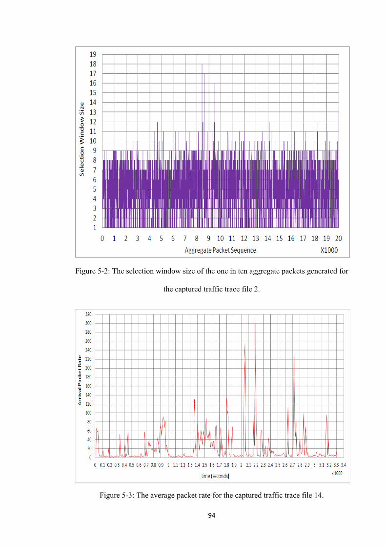
94
Figure 5-2: The selection window size of the one in ten aggregate packets generated for
the captured traffic trace file 2.
Figure 5-3: The average packet rate for the captured traffic trace file 14.

95
Figure 5-4: The selection window size for the aggregate packets generated for all raw
packets input for the captured traffic trace file 14.
5.1.2 CCDF of the Number of Sub-packets
The CCDF of the number of sub-packets is the probability that the number of sub-
packets has a value greater than or equal to a certain value. The CCDF allows us to
compare the performances in terms of the average number of sub-packets per aggregate
packet for the different algorithms. The CCDF of the number of sub-packets for the
captured traffic trace file 2 is shown in Figure 5-5 and that for the captured traffic trace
file 14 is shown in Figure 5-6.
As shown in Figure 5-5, Figure 5-6 and in appendix B, the captured traffic trace files
are tested in a number of different cases:
(1) The FIFO algorithm;
(2) The SSFS algorithm;
(3) The AAM algorithm;
(4) The AAM algorithm with a fixed selection window size at 3, 8 and 10.

96
Figure 5-5: The CCDF of the number of sub-packets for the captured traffic trace file 2.
From the result for the FIFO algorithm in Figure 5-5, over 50% of the aggregate packets
contain just 1 sub-packet and the probability is less than 0.1 that the number of sub-
packets is greater than 2. While for the AAM algorithm, the probability is over 0.6 that
the number of sub-packets is greater than 2. This indicates that the average number of
sub-packets per aggregate packet produced by the AAM algorithm is greater than that
generated by the FIFO algorithm. The performance in terms of the CCDF of the number
of sub-packets for the SSFS algorithm is the best for all three algorithms considered.
This means that the SSFS algorithm produces the largest average number of sub-packets
per aggregate packet and the FIFO algorithm produces the smallest average number of
sub-packets per aggregate packet.
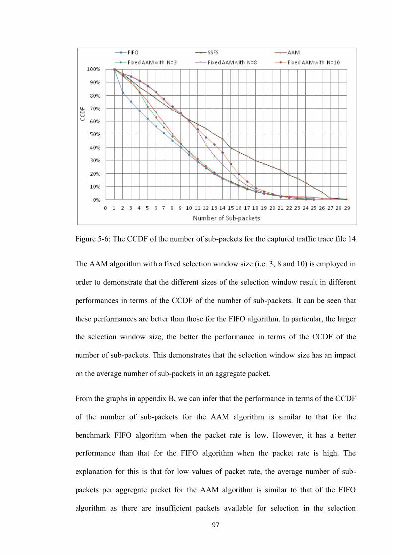
97
Figure 5-6: The CCDF of the number of sub-packets for the captured traffic trace file 14.
The AAM algorithm with a fixed selection window size (i.e. 3, 8 and 10) is employed in
order to demonstrate that the different sizes of the selection window result in different
performances in terms of the CCDF of the number of sub-packets. It can be seen that
these performances are better than those for the FIFO algorithm. In particular, the larger
the selection window size, the better the performance in terms of the CCDF of the
number of sub-packets. This demonstrates that the selection window size has an impact
on the average number of sub-packets in an aggregate packet.
From the graphs in appendix B, we can infer that the performance in terms of the CCDF
of the number of sub-packets for the AAM algorithm is similar to that for the
benchmark FIFO algorithm when the packet rate is low. However, it has a better
performance than that for the FIFO algorithm when the packet rate is high. The
explanation for this is that for low values of packet rate, the average number of sub-
packets per aggregate packet for the AAM algorithm is similar to that of the FIFO
algorithm as there are insufficient packets available for selection in the selection

98
window. While for large values of packet rate, the average number of sub-packets per
aggregate packet for the AAM algorithm is larger than that for the FIFO algorithm as
there are sufficient packets available for selection in the selection window.
The performance in terms of the CCDF of the number of sub-packets for the AAM
algorithm is always poorer than that for the SSFS algorithm as the SSFS algorithm tries
to aggregate as many sub-packets as possible associated with a large delay.
5.1.3 CDF of the Sub-packet Delay
The CDF of the sub-packet delay represents the probability that the sub-packet delay
takes on a value less than or equal to a certain value which allows us to compare the
performance in terms of the average sub-packet delay for the different algorithms. The
CDF of the sub-packet delay for all three algorithms considered SSFS, FIFO and AAM
are shown in Figure 5-7 and Figure 5-8 for the captured traffic trace files 2 and 14
respectively.
From the two graphs, it can be seen that the benchmark FIFO algorithm has the best
performance in terms of the CDF of the sub-packet delay and the performance for the
AAM algorithm is poorer than that of the FIFO algorithm, but it is better than that of the
SSFS algorithm. This means that the average sub-packet delay for the FIFO algorithm is
the lowest and for the SSFS algorithm is the largest. As shown in Figure 5-7, the sub-
packet delays are less than 0.05 seconds for over 90% of the sub-packets for the FIFO
algorithm and 80% of the sub-packets for the AAM algorithm, while only 20% of the
sub-packets for the SSFS algorithm. However, in Figure 5-8, the number of sub-packets
whose delay is less than 0.05 seconds is reduced to 60% for the FIFO algorithm, 50%
for the AAM algorithm and 10% for the SSFS algorithm.

99
Figure 5-7: The CDF of the sub-packet delay for the captured traffic trace file 2.
Figure 5-8: The CDF of the sub-packet delay for the captured traffic trace file 14.
By observing the results in appendix C, it can be seen that when the packet rate is low,
the performances in terms of the CDF of the sub-packet delay for the AAM and FIFO
algorithms are similar. However, they still have a superior performance over the SSFS
algorithm in terms of the CDF of the sub-packet delay. This means that the average sub-
packet delay for the AAM algorithm is similar to that for the FIFO algorithms but it is
smaller than that for the SSFS algorithm when the packet rate is low as the AAM
algorithm may need a longer time to wait for the packets to arrive. It also shows that the
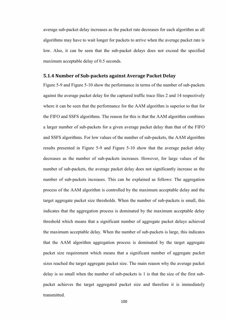
100
average sub-packet delay increases as the packet rate decreases for each algorithm as all
algorithms may have to wait longer for packets to arrive when the average packet rate is
low. Also, it can be seen that the sub-packet delays does not exceed the specified
maximum acceptable delay of 0.5 seconds.
5.1.4 Number of Sub-packets against Average Packet Delay
Figure 5-9 and Figure 5-10 show the performance in terms of the number of sub-packets
against the average packet delay for the captured traffic trace files 2 and 14 respectively
where it can be seen that the performance for the AAM algorithm is superior to that for
the FIFO and SSFS algorithms. The reason for this is that the AAM algorithm combines
a larger number of sub-packets for a given average packet delay than that of the FIFO
and SSFS algorithms. For low values of the number of sub-packets, the AAM algorithm
results presented in Figure 5-9 and Figure 5-10 show that the average packet delay
decreases as the number of sub-packets increases. However, for large values of the
number of sub-packets, the average packet delay does not significantly increase as the
number of sub-packets increases. This can be explained as follows: The aggregation
process of the AAM algorithm is controlled by the maximum acceptable delay and the
target aggregate packet size thresholds. When the number of sub-packets is small, this
indicates that the aggregation process is dominated by the maximum acceptable delay
threshold which means that a significant number of aggregate packet delays achieved
the maximum acceptable delay. When the number of sub-packets is large, this indicates
that the AAM algorithm aggregation process is dominated by the target aggregate
packet size requirement which means that a significant number of aggregate packet
sizes reached the target aggregate packet size. The main reason why the average packet
delay is so small when the number of sub-packets is 1 is that the size of the first sub-
packet achieves the target aggregated packet size and therefore it is immediately
transmitted.

101
Figure 5-9: The number of sub-packets against the average packet delay for the captured
traffic trace file 2.
Figure 5-10: The number of sub-packets against the average packet delay for the
captured traffic trace file 14.
The two figures have quite different shapes as the two captured traffic trace files have
different packet rates which are shown in Table 4-2. The packet rate of the captured
traffic trace file 2 is 114 pps while it is 19.2 pps for the captured traffic trace file 14.
From all the graphs for the 16 captured traffic trace files presented in appendix D, when

102
the packet rate is large, the performance in terms of the number of sub-packets against
the average packet delay for the AAM algorithm is the best for all three algorithms
considered. For low values of the packet rate, the performance for the AAM algorithm
is similar to that for the FIFO algorithm as the number of sub-packets that can be
combined into an aggregate packet by the AAM algorithm is similar to that for the
FIFO algorithm because there are insufficient packets available for selection from the
selection window.
5.1.5 Conclusion
The performances in terms of the selection window size, the CCDF of the number of
sub-packets, the CDF of the sub-packet delay and the number of sub-packets against the
average packet delay for all three algorithms considered have been presented. The
following conclusions can be drawn:
The AAM algorithm is an adaptive algorithm which can operate over a wide
range of different traffic loads. The selection window size is adaptively adjusted
to follow the variations in the packet rate of the traffic load. The size of the
selection window has an impact on the performance in terms of the CCDF of
the number of sub-packets. In particular, the larger the size of the selection
window, the better the performance in terms of the CCDF of the number of sub-
packets.
The AAM algorithm has a better performance in terms of the CCDF of the
number of sub-packets than that for the benchmark FIFO algorithm but is
poorer than that for the SSFS algorithm. This means that the average number of
sub-packets per aggregate packet generated by the AAM algorithm is larger
than that for the FIFO algorithm but is smaller than that for the SSFS algorithm.

103
The AAM algorithm has a better performance in terms of the CDF of the sub-
packet delay than that for the SSFS algorithm but is poorer than that for the
FIFO algorithm. This means that the AAM algorithm has a shorter average sub-
packet delay than that for the SSFS algorithm but is longer than that for the
FIFO algorithm.
The performance in terms of the number of sub-packet against the average
packet delay for the AAM algorithm is the best for all three algorithms
considered. This means that the AAM algorithm can aggregate a larger number
of sub-packets for a given average packet delay than the other two algorithms
considered due to its adaptive nature. However, when the packet rate is low, the
performance for the AAM algorithm is similar to that for the FIFO algorithm as
there are insufficient packets available for selection in the selection window.
5.2 Performance in Wireless Networks
In this section, we will present the results for the AAM algorithm implemented in a
wireless network test scenario which was described in chapter 4. The performance of
the FIFO and SSFS algorithms will also be shown. In this test scenario, the AAM
algorithm is implemented in a wireless network under two different operating
environments. The first one is an ideal environment where transmission errors are
absent and the PHY rate adaption mechanism is also disabled and the other one is the
same wireless network but with transmission errors present where the PHY rate
adaption mechanism is employed. The objective of this test scenario is to demonstrate
that the AAM algorithm has a superior performance over the other two algorithms in
terms of the aggregation trade-off. It is also to demonstrate that the AAM algorithm is a
robust algorithm which has a superior performance over the other two algorithms in
terms of the throughput in error-prone wireless networks.
104
5.2.1 Performance in an Ideal Wireless Network
The AAM, FIFO and SSFS algorithms were implemented in an ns-3 simulation wireless
network where transmission errors are absent and the PHY rate adaption mechanism is
disabled. In this scenario, as described in section 4.6.2, the DataRate parameter of
OnOffApplication is modified in order to change the data rate by changing the interval
between the raw packets of the captured traffic trace files. The interval can be changed
by using the OffTime parameter of OnOffApplication module. Figure 5-11 and Figure
5-12 show the performances in terms of the throughput against the data rate for the
different IEEE 802.11 PHY rates for the captured traffic trace files 2 and 14
respectively. It can be seen that the AAM algorithm has the best performance in terms
of the throughput for the 8 different PHY rates for all three algorithms considered. The
FIFO algorithm has the poorest performance in terms of the throughput. The
improvement in the throughput increases as the PHY rate increases. When the PHY rate
is 6 Mbps, the throughput improvement is 6% compared with 30% when the PHY rate
is 54 Mbps for the AAM compared to the FIFO algorithm. For example, as shown in
Figure 5-11, when the PHY rate is fixed at 54 Mbps, the maximum throughput for the
FIFO algorithm is 20 Mbps and for the SSFS algorithm it is 23 Mbps, while the
maximum throughput for the AAM algorithm is as large as 26 Mbps. This is because
the AAM algorithm can combine a larger number of packets per aggregate packet for a
given delay in wireless networks where the delay is defined as the maximum acceptable
delay.
From Figure 5-11 and Figure 5-12, it can be seen that when the PHY rate is fixed and
the data rate is low, the AAM, FIFO and SSFS algorithms have similar performances in
terms of their throughput. However, if the data rate is large, the AAM algorithm has a
superior performance compared to the other two algorithms in terms of the throughput.
For example, when the data rate is below 19 Mbps with a PHY rate fixed at 54 Mbps,

105
the performances in terms of the throughput are similar for all three algorithms
considered; while if the data rate is greater than 23 Mbps, the throughput for the AAM
algorithm is greater than that of both the FIFO and SSFS algorithms. The reason is that
when the data rate is low, the performance of the AAM algorithm degrades to that for
the FIFO algorithm as there are insufficient packets to be selected from the selection
window. When the data rate is large, there are sufficient packets for selection in the
selection window to generate a larger size aggregate packet for a given delay by the
AAM algorithm.
Figure 5-11: The throughput against data rate for the different PHY rates for the
captured traffic trace file 2.
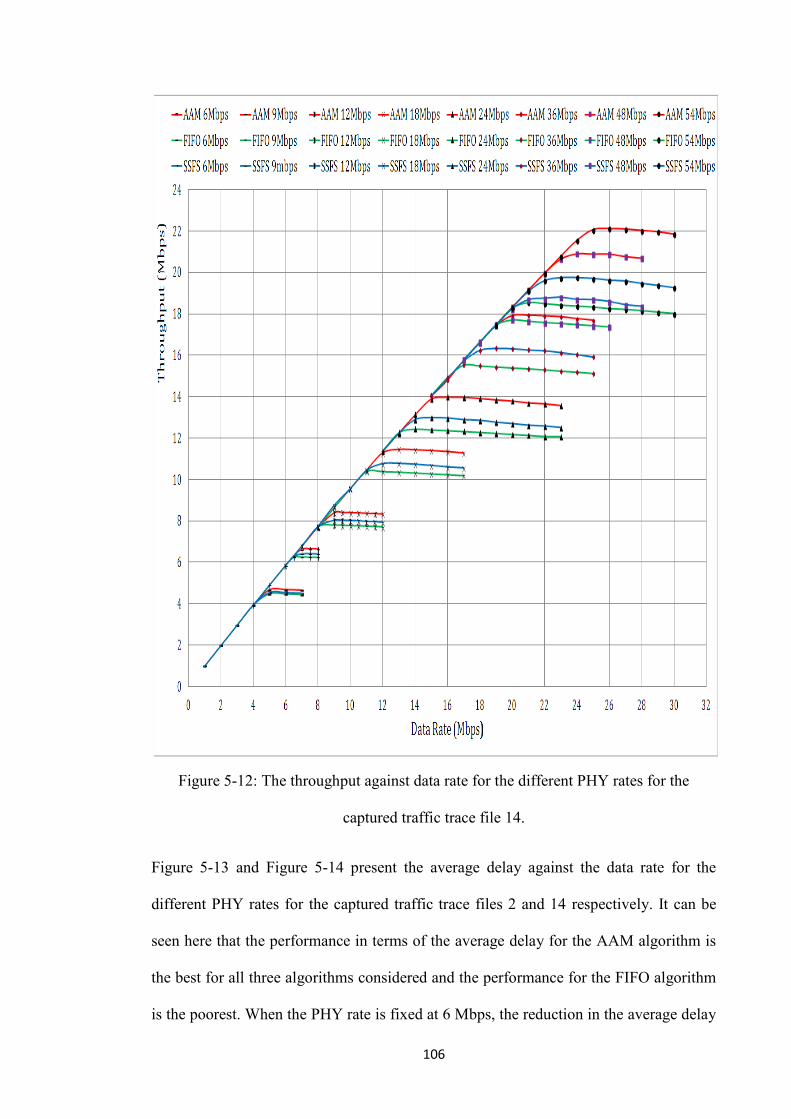
106
Figure 5-12: The throughput against data rate for the different PHY rates for the
captured traffic trace file 14.
Figure 5-13 and Figure 5-14 present the average delay against the data rate for the
different PHY rates for the captured traffic trace files 2 and 14 respectively. It can be
seen here that the performance in terms of the average delay for the AAM algorithm is
the best for all three algorithms considered and the performance for the FIFO algorithm
is the poorest. When the PHY rate is fixed at 6 Mbps, the reduction in the average delay
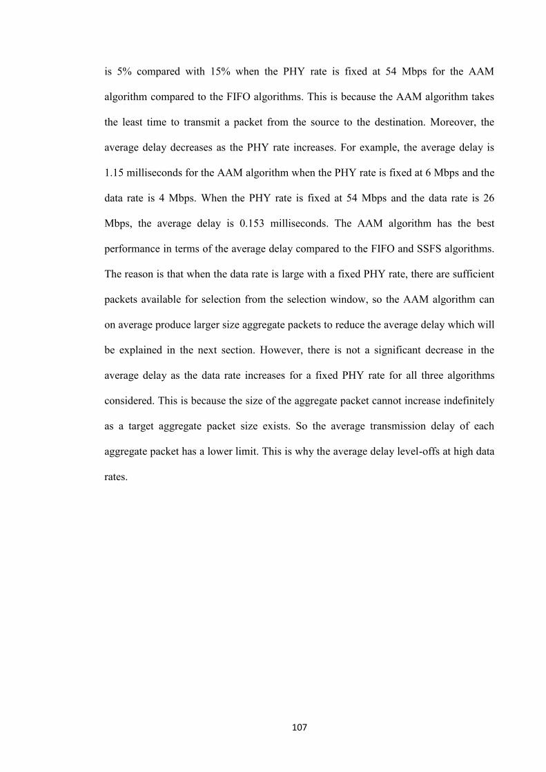
107
is 5% compared with 15% when the PHY rate is fixed at 54 Mbps for the AAM
algorithm compared to the FIFO algorithms. This is because the AAM algorithm takes
the least time to transmit a packet from the source to the destination. Moreover, the
average delay decreases as the PHY rate increases. For example, the average delay is
1.15 milliseconds for the AAM algorithm when the PHY rate is fixed at 6 Mbps and the
data rate is 4 Mbps. When the PHY rate is fixed at 54 Mbps and the data rate is 26
Mbps, the average delay is 0.153 milliseconds. The AAM algorithm has the best
performance in terms of the average delay compared to the FIFO and SSFS algorithms.
The reason is that when the data rate is large with a fixed PHY rate, there are sufficient
packets available for selection from the selection window, so the AAM algorithm can
on average produce larger size aggregate packets to reduce the average delay which will
be explained in the next section. However, there is not a significant decrease in the
average delay as the data rate increases for a fixed PHY rate for all three algorithms
considered. This is because the size of the aggregate packet cannot increase indefinitely
as a target aggregate packet size exists. So the average transmission delay of each
aggregate packet has a lower limit. This is why the average delay level-offs at high data
rates.
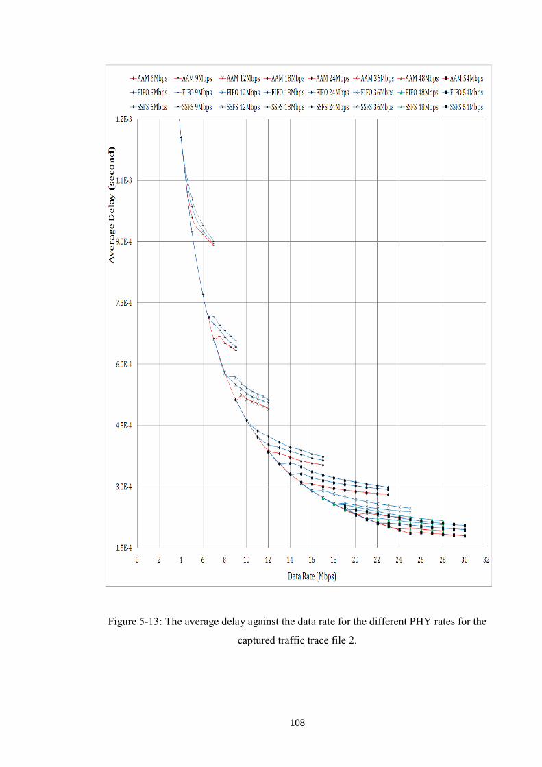
108
Figure 5-13: The average delay against the data rate for the different PHY rates for the
captured traffic trace file 2.
109
Figure 5-14: The average delay against the data rate for the different PHY rates for the
captured traffic trace file 14.
Figure 5-15 and Figure 5-16 present the performance in terms of the average aggregate
packet size for the different PHY rates under saturation for all three algorithms
considered. It can be seen that the AAM algorithm has the largest average aggregate
packet size for the different PHY rates in saturated wireless networks, while the FIFO
algorithm has the smallest average aggregate packet size. It can be seen that the AAM
algorithm can improve the average aggregate packet size by as much as 50% compared
to the FIFO algorithm for the captured trace file 2 as the average size of an AAM
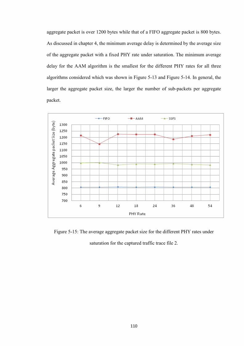
110
aggregate packet is over 1200 bytes while that of a FIFO aggregate packet is 800 bytes.
As discussed in chapter 4, the minimum average delay is determined by the average size
of the aggregate packet with a fixed PHY rate under saturation. The minimum average
delay for the AAM algorithm is the smallest for the different PHY rates for all three
algorithms considered which was shown in Figure 5-13 and Figure 5-14. In general, the
larger the aggregate packet size, the larger the number of sub-packets per aggregate
packet.
Figure 5-15: The average aggregate packet size for the different PHY rates under
saturation for the captured traffic trace file 2.
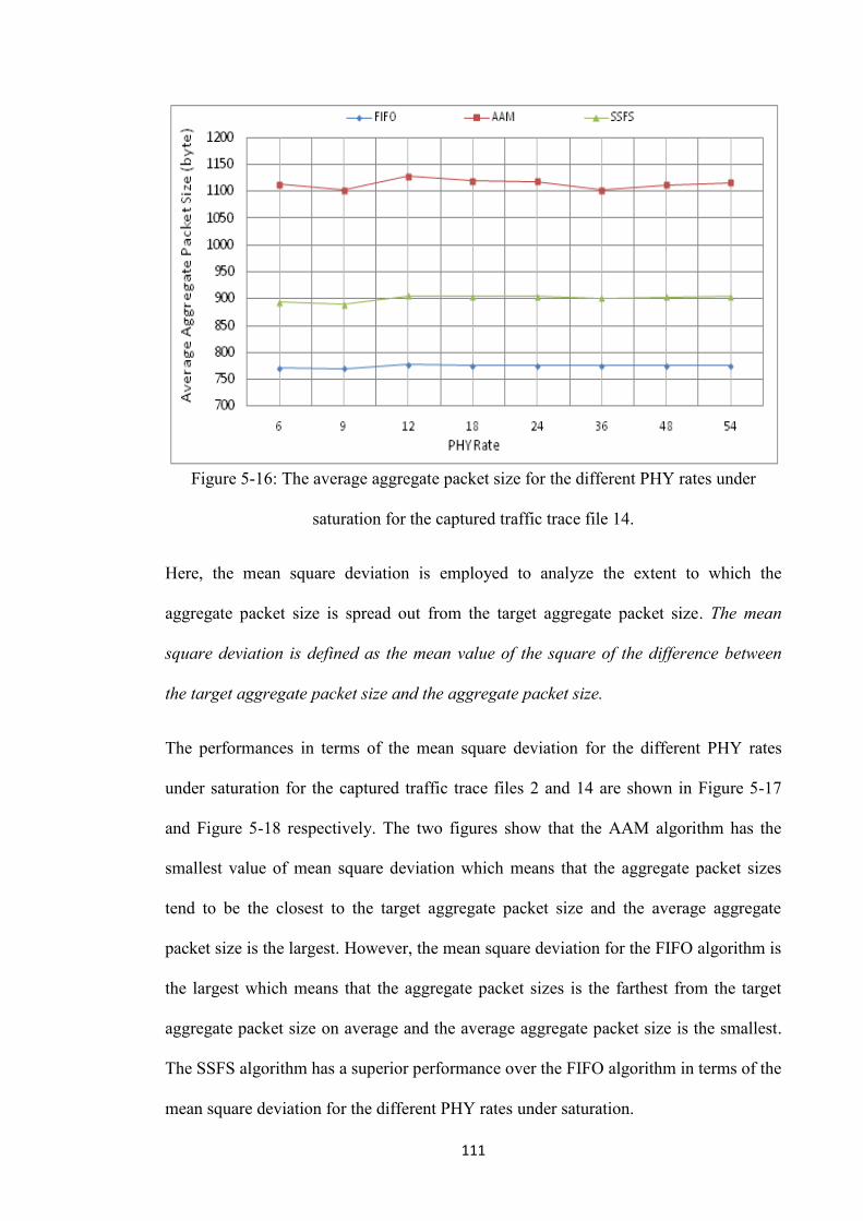
111
Figure 5-16: The average aggregate packet size for the different PHY rates under
saturation for the captured traffic trace file 14.
Here, the mean square deviation is employed to analyze the extent to which the
aggregate packet size is spread out from the target aggregate packet size. The mean
square deviation is defined as the mean value of the square of the difference between
the target aggregate packet size and the aggregate packet size.
The performances in terms of the mean square deviation for the different PHY rates
under saturation for the captured traffic trace files 2 and 14 are shown in Figure 5-17
and Figure 5-18 respectively. The two figures show that the AAM algorithm has the
smallest value of mean square deviation which means that the aggregate packet sizes
tend to be the closest to the target aggregate packet size and the average aggregate
packet size is the largest. However, the mean square deviation for the FIFO algorithm is
the largest which means that the aggregate packet sizes is the farthest from the target
aggregate packet size on average and the average aggregate packet size is the smallest.
The SSFS algorithm has a superior performance over the FIFO algorithm in terms of the
mean square deviation for the different PHY rates under saturation.
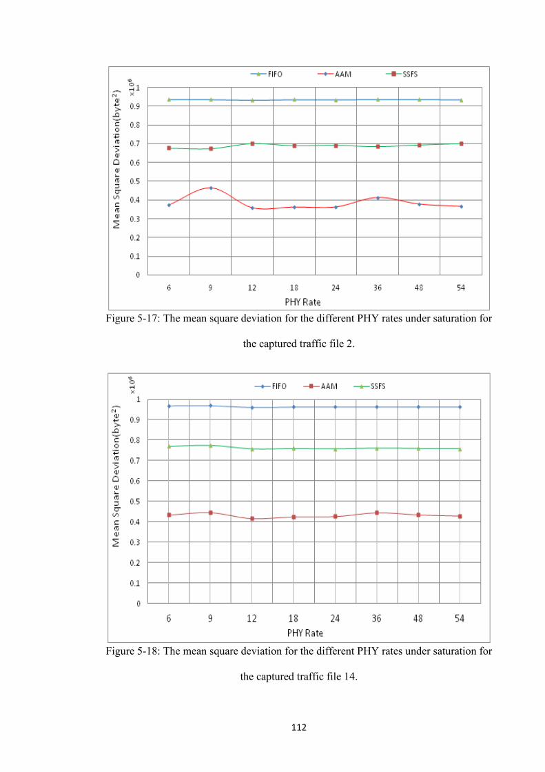
112
Figure 5-17: The mean square deviation for the different PHY rates under saturation for
the captured traffic file 2.
Figure 5-18: The mean square deviation for the different PHY rates under saturation for
the captured traffic file 14.
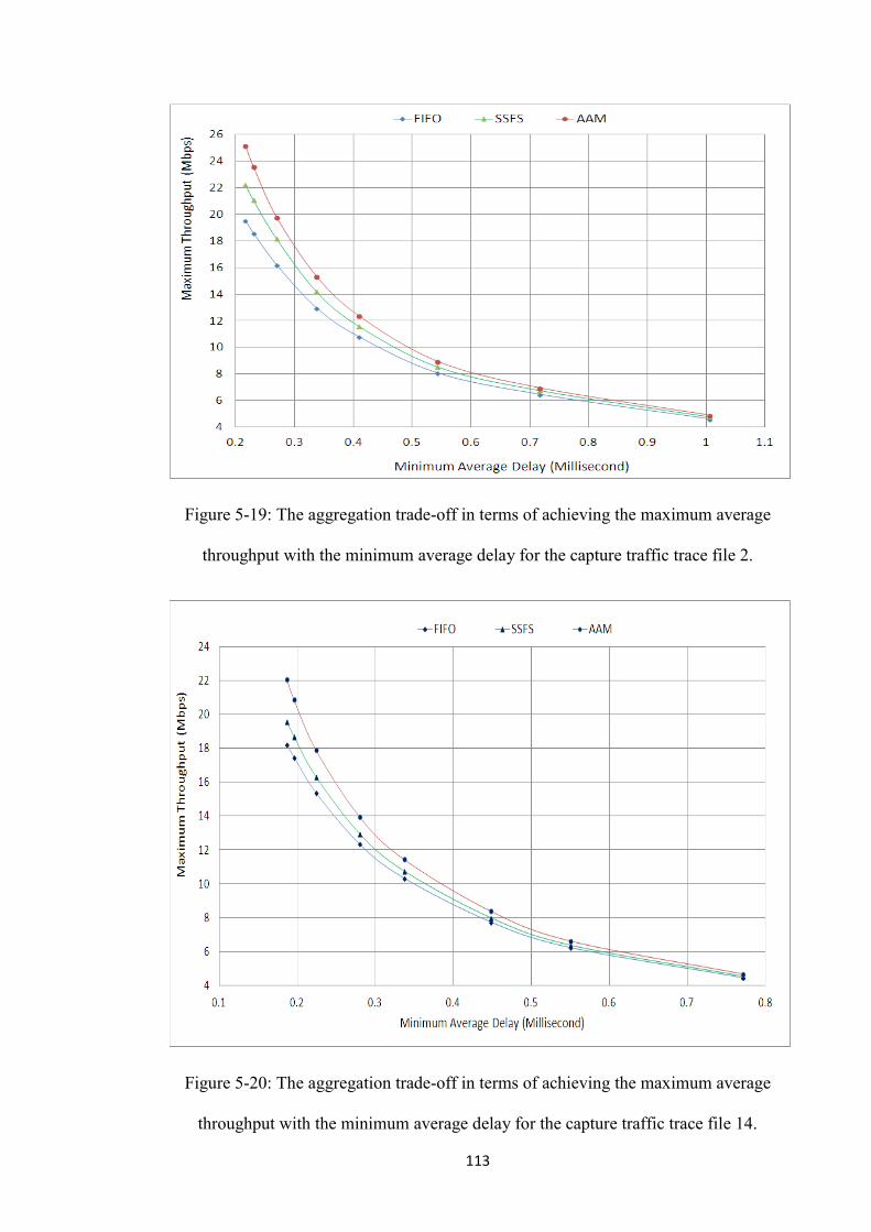
113
Figure 5-19: The aggregation trade-off in terms of achieving the maximum average
throughput with the minimum average delay for the capture traffic trace file 2.
Figure 5-20: The aggregation trade-off in terms of achieving the maximum average
throughput with the minimum average delay for the capture traffic trace file 14.

114
Figure 5-19 and Figure 5-20 show the performance in terms of the aggregation trade-off
in achieving the maximum average throughput with the minimum average delay for the
captured traffic trace files 2 and 14 respectively. It can be seen here that the AAM
algorithm has the best performance in terms of the aggregation trade-off due to the
adaptive nature of the AAM algorithm. As the minimum average delay is dependent
upon the PHY rate, a low value of the minimum average delay corresponds to a large
PHY rate. From these two figures, it can be seen that the improvement in the
aggregation trade-off increases as the PHY rate increases. When the PHY rate is large
(i.e. for a low value of minimum average delay), the aggregation trade-off improvement
is the best for the AAM algorithm compared to the other two algorithms as the AAM
algorithm can successfully transmit more data for a given minimum average delay.
When the PHY rate is low (i.e. for a large value of minimum average delay), the
performance in terms of aggregation trade-off for the AAM algorithm is similar to that
for the other two algorithms. This shows that when the PHY rate is low, the AAM
algorithm still can improve the performance in terms of aggregation trade-off compared
to the FIFO algorithm but cannot significantly improve it.
Conclusion
Based on the previous discussions for the AAM algorithm implemented in a wireless
network without transmission errors present and with the PHY rate adaption mechanism
disabled, a number of conclusions can be draw:
The AAM algorithm has the best performance in terms of the throughput for all
three algorithms considered and the improvement in the throughput increases as
the PHY rate increases. It improves the throughout from 6% with a PHY rate
fixed at 6 Mbps up to 30% with a PHY rate fixed at 54 Mbps compared to the
FIFO algorithm.

115
The AAM algorithm has a similar performance to the other algorithms in terms
of the throughput when the data rate is low with a fixed PHY rate. The reason is
that the wireless network is unsaturated which can be determined by checking
the AAM algorithm to see if it needs to wait for further packet arrival or not. If it
needs to do it, the network is unsaturated. When the data rate is large, the AAM
algorithm has a superior performance over the other algorithms in terms of the
throughput as there are sufficient packets for selection from the selection
window to generate a larger size aggregate packet for a given delay.
The AAM algorithm has the best performance in terms of the average delay. The
AAM algorithm has the best performance in terms of the average delay for all
three algorithms considered and it reduces the average delay by up to 15%
compared to the FIFO algorithm with a PHY rate at 54 Mbps. The average delay
decreases as the PHY rate increases for all three algorithms considered.
The AAM algorithm has the best performances in terms of the average
aggregate packet size and the mean square deviation under saturation for all
three algorithms considered. The average size of an AAM aggregate packet is
1.5 times that for a FIFO aggregate packet. This demonstrates that the AAM
algorithm produces the largest average size of the aggregate packet. The AAM
algorithm has the smallest value of the mean square deviation which
demonstrates that it has the largest number of aggregate packets whose sizes are
closest to the target aggregate packet size.
The AAM algorithm has the best performance in terms of the aggregation trade-
off in achieving the maximum average throughput with the minimum average
delay for all three algorithms considered as it achieves the largest throughput at
the cost of the least average delay.

116
5.2.2 Performance in an Error-Prone Wireless Network
The AAM, SSFS and FIFO algorithms are implemented in the same wireless network
simulation but with transmission errors present and the PHY rate adaption mechanism
enabled. The transmission errors are characterized by the BER and the PHY rate
adaption mechanism is implemented by the AarfWifiManager module in the ns-3
simulator. As described in chapter 4, the objective of the PHY rate adaption mechanism
is to improve the throughput by selecting the most effective PHY rate to transmit the
frames. However, in this case it will be shown that the AARF mechanism is not the
main factor contributing to the throughput improvement when using the AAM
algorithm.
Figure 5-21: The throughput against data rate for the different BERs for the captured
trace file 2.
Figure 5-21 and Figure 5-22 show the performance in terms of the throughput against
data rate for the different BERs (i.e. 10-4
, 10-3
and 5×10⁻³
) for the captured traffic trace
files 2 and 14 respectively. The graphs show that the throughput improvement increases
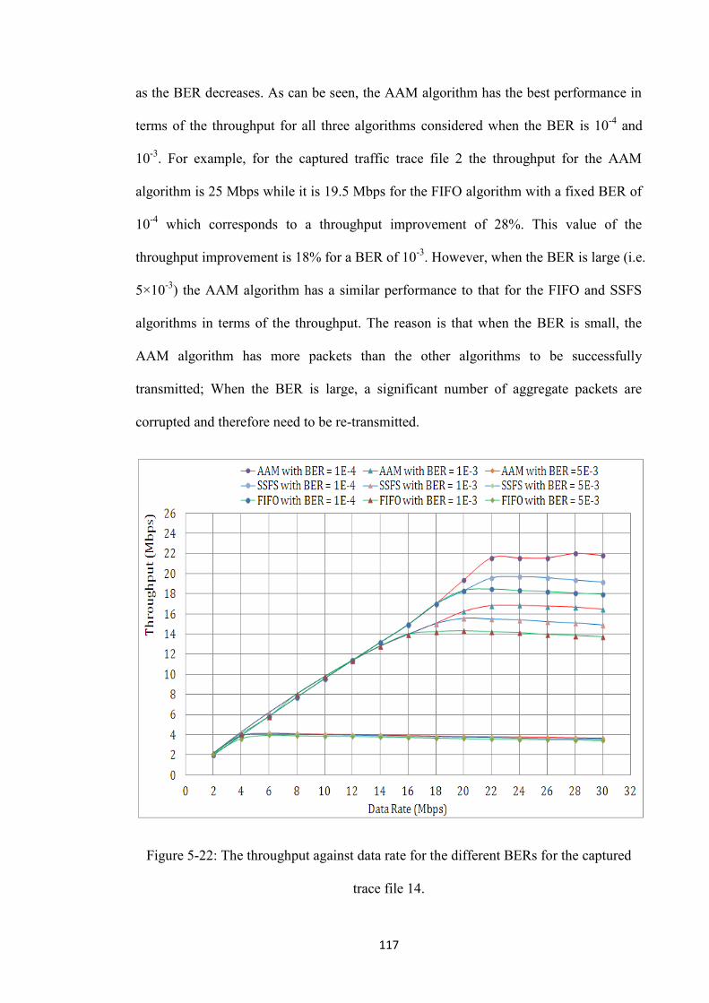
117
as the BER decreases. As can be seen, the AAM algorithm has the best performance in
terms of the throughput for all three algorithms considered when the BER is 10-4
and
10-3
. For example, for the captured traffic trace file 2 the throughput for the AAM
algorithm is 25 Mbps while it is 19.5 Mbps for the FIFO algorithm with a fixed BER of
10-4
which corresponds to a throughput improvement of 28%. This value of the
throughput improvement is 18% for a BER of 10-3
. However, when the BER is large (i.e.
5×10⁻³
) the AAM algorithm has a similar performance to that for the FIFO and SSFS
algorithms in terms of the throughput. The reason is that when the BER is small, the
AAM algorithm has more packets than the other algorithms to be successfully
transmitted; When the BER is large, a significant number of aggregate packets are
corrupted and therefore need to be re-transmitted.
Figure 5-22: The throughput against data rate for the different BERs for the captured
trace file 14.
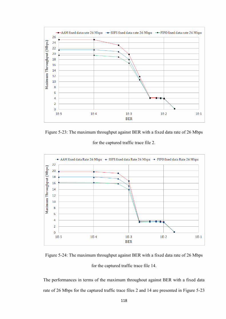
118
Figure 5-23: The maximum throughput against BER with a fixed data rate of 26 Mbps
for the captured traffic trace file 2.
Figure 5-24: The maximum throughput against BER with a fixed data rate of 26 Mbps
for the captured traffic trace file 14.
The performances in terms of the maximum throughout against BER with a fixed data
rate of 26 Mbps for the captured traffic trace files 2 and 14 are presented in Figure 5-23
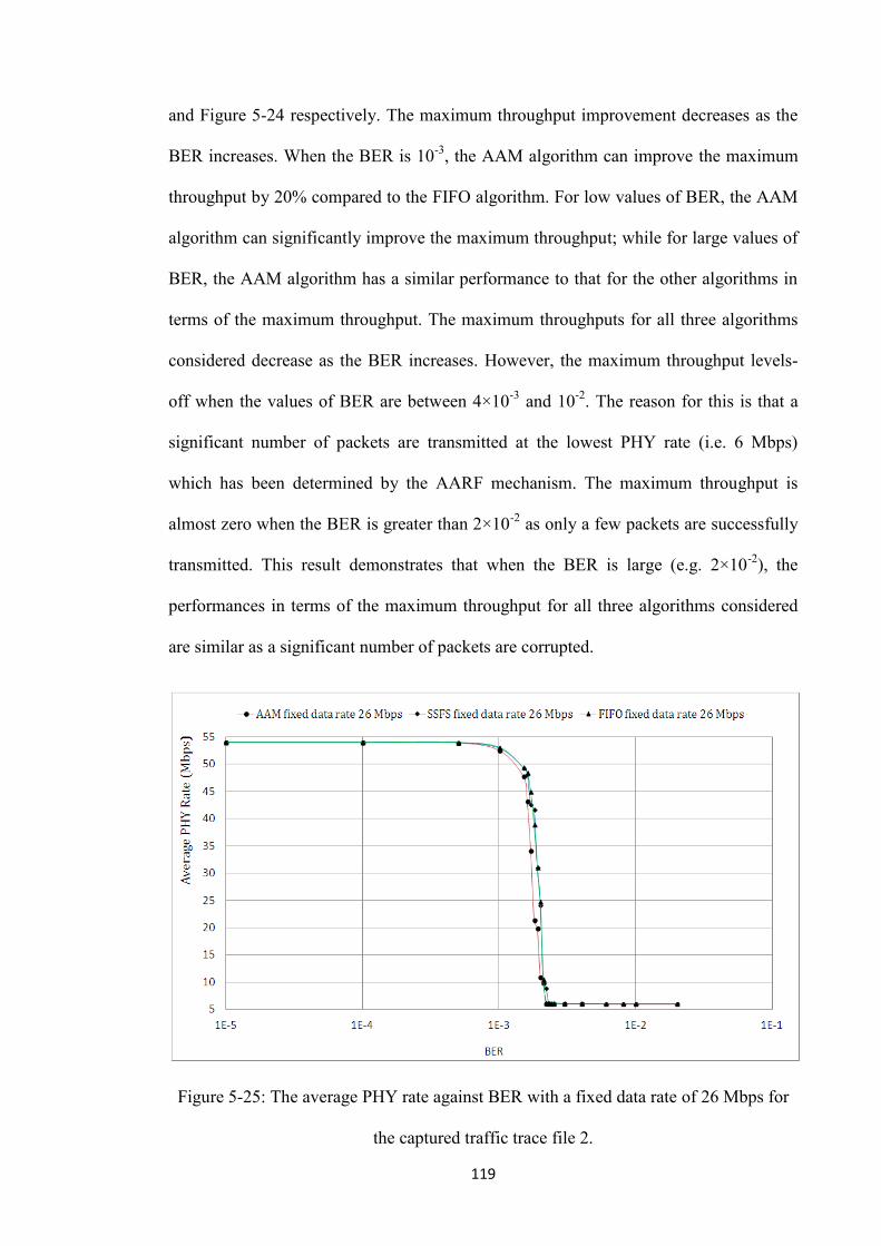
119
and Figure 5-24 respectively. The maximum throughput improvement decreases as the
BER increases. When the BER is 10-3
, the AAM algorithm can improve the maximum
throughput by 20% compared to the FIFO algorithm. For low values of BER, the AAM
algorithm can significantly improve the maximum throughput; while for large values of
BER, the AAM algorithm has a similar performance to that for the other algorithms in
terms of the maximum throughput. The maximum throughputs for all three algorithms
considered decrease as the BER increases. However, the maximum throughput levels-
off when the values of BER are between 4×10⁻³
and 10-2
. The reason for this is that a
significant number of packets are transmitted at the lowest PHY rate (i.e. 6 Mbps)
which has been determined by the AARF mechanism. The maximum throughput is
almost zero when the BER is greater than 2×10⁻²
as only a few packets are successfully
transmitted. This result demonstrates that when the BER is large (e.g. 2×10⁻²
), the
performances in terms of the maximum throughput for all three algorithms considered
are similar as a significant number of packets are corrupted.
Figure 5-25: The average PHY rate against BER with a fixed data rate of 26 Mbps for
the captured traffic trace file 2.

120
Figure 5-26: The average PHY rate against BER with a fixed data rate of 26 Mbps for
the captured traffic trace file 14.
The performances in terms of the average PHY rate against BER with a fixed data rate
of 26 Mbps for the captured traffic trace files 2 and 14 are presented in Figure 5-25 and
Figure 5-26 respectively. It can be clearly seen that the performances in terms of the
average PHY rates are similar for all three algorithms considered. When the BER is less
than 10-3
the PHY rate is close to 54 Mbps and the PHY rate is almost 6 Mbps if the
BER is greater than 4×10⁻³
. The PHY rate sharply decreases from 54 Mbps to 6 Mbps
when the BER increases from 10-3
to 4×10⁻³
. The result shows that the PHY rate
adaption mechanism AARF is not the main factor contributing to the improvement in
the throughput by using the AAM algorithm but rather the adaptive nature of the AAM
algorithm.
Conclusion
Based on the previous discussions for the AAM algorithm implemented in a wireless
network with transmission errors present and with the PHY rate adaption mechanism
enabled, the following conclusions can be draw:

121
The AAM algorithm has a superior performance compared to the other two
algorithms in terms of the throughput. Moreover, the improvement in the
throughput decreases as the BER increases. When the BER is 10-4
, the AAM
algorithm improves the throughput by 28%, while it cannot significantly
improve the throughput when the BER is large (i.e. 5×10⁻³
).
The PHY rate adaption mechanism AARF is not the main factor responsible for
the improvement in the throughput as the performances are similar for all three
algorithms considered in terms of the average PHY rate against BER with a
fixed data rate of 26 Mbps. The main factor that contributes to the improvement
in the throughput is the adaptive nature of the AAM algorithm.
5.3 Chapter Summary
In this chapter the main findings of the analysis of the AAM algorithm implemented in
two test scenarios have been presented. The performance of the AAM algorithm
implemented in the first scenario involving the aggregation process only demonstrated
that the AAM algorithm is an adaptive packet aggregation algorithm which can operate
over a wide range of different traffic loads by employing a tunable selection window
scheme and a hybrid selection strategy. An analysis of the CCDF of the number of sub-
packets and the CDF of the sub-packet delay demonstrated that the AAM algorithm has
a superior performance compared to the FIFO and SSFO algorithms.
The AAM algorithm also has the best performance in terms of the number of sub-
packets against the average packet delay as it can combine a larger number of sub-
packets per aggregate packet for a given average packet delay. It was also shown that
when the packet rate is low, the performances are similar in terms of the number of sub-
packets against the average packet delay as the performance for the AAM algorithm
degrades towards that for the FIFO algorithm.
122
The results of the second scenario where the AAM algorithm has been deployed in a
simulated wireless network with and without transmission errors present were presented.
In the ideal wireless network (i.e. without transmission errors present) where the PHY
rate adaption mechanism is not employed, the AAM algorithm has the best performance
in terms of the throughput and the average delay for the different IEEE 802.11 PHY
rates. The AAM algorithm can improve the throughput by 30% and reduce the average
delay by 15% compared to the FIFO algorithm with a fixed PHY rate of 54 Mbps.
However, when the data rate is low with a fixed PHY rate, the performances are similar
in terms of the throughput and the average delay for all three algorithms considered.
The performances in terms of the average aggregate packet size and the mean square
deviation for the AAM algorithm are the best for all three algorithms considered. The
AAM algorithm also has the best performance in terms of the aggregation trade-off in
achieving the maximum average throughput with the minimum average delay for all
three algorithms considered. The improvement in this performance increases as the
PHY rate increases. When the PHY rate is 6 Mbps, the performances are similar in
terms of the aggregation trade-off in achieving the maximum average throughput with
the minimum average delay for all three algorithms considered.
In the case of a wireless network with transmission errors present where the PHY rate
adaption mechanism is employed, the AAM algorithm has the best performance in
terms of the throughput when the BER is low. The AAM algorithm can improve the
throughput by 28% compared to the FIFO algorithm when the BER is 10-4
. The
improvement in the throughput decreases as the BER increases. When the BER is 10-3
,
the AAM algorithm can improve the throughout by 20% compared to the FIFO
algorithm. However, the throughputs are almost zero for all three algorithms considered
when the BER is 2×10⁻²
. Therefore the AAM algorithm cannot provide any significant
benefits in a simulated wireless networks with large values of BER as a significant
123
number of packets are corrupted and need to be re-transmitted. Furthermore, the results
demonstrate that the PHY rate adaption mechanism is not the main factor contributing
to the improvement in the throughput but rather the adaptive nature of the AAM
algorithm.
124
Chapter 6 Conclusions and Future Work
Packet aggregation is a technique which combines a number of data packets into a
single large data packet in order to achieve higher throughputs by reducing the overhead
associated with protocol headers in packet-based communications networks. In the
IEEE 802.11n standard, two packet aggregation algorithms have been proposed to
improve the throughput: A-MSDU and A-MPDU. However, a packet aggregation
algorithm can also increase the delay as it may need to wait for more packets to arrive in
order to be aggregated into an aggregate packet. Consequently, there exists a trade-off
between the throughput and the delay for all packet aggregation algorithms. However,
most of the packet aggregation algorithms proposed so far just tend to optimize a single
metric, i.e. either to maximize throughput or to minimize delay. In other words, they do
not take account of the varying nature of the mixed traffic load particularly the random
nature of the packet size and inter-arrival time.
In this thesis, an adaptive packet aggregation algorithm called the Adaptive Aggregation
Mechanism (AAM) has been proposed to achieve the best aggregation trade-off in
realizing the maximum average throughput with the minimum average delay compared
to two other packet aggregation algorithms (i.e. FIFO and SSFS) for different traffic
loads. The AAM algorithm is essentially a feedback control system that can operate
over a wide range of different traffic loads by employing an adaptive selection window
mechanism and a hybrid selection strategy. There are three elements to the AAM
algorithm: Adjustable Aggregation Algorithm (A3), Aggregate Packer Analyzer (APA)
and Aggregate Tuning Algorithm (ATA). The A3
selects packets from the selection
window in the input buffer based on a hybrid selection strategy and then aggregates
them together in the output buffer. The hybrid selection strategy results in the first sub-

125
packet being selected based on the packet arrival time and the other sub-packets being
selected based on the packet size. The selection window size can be adaptively adjusted.
The APA analyses the number of sub-packets and the aggregate packet delay between
the current and previous aggregate packet. The ATA determines the size of the selection
window for the next aggregate packet based on the analysis results from the APA. The
aggregation process is determined by two user specified threshold values: the target
aggregate packet size and the maximum acceptable delay.
In order to demonstrate the performance for the AAM algorithm over a wide range of
different traffic loads, there were 16 traffic trace files used which were captured from a
number of live Wi-Fi hotspot networks at different times and locations. These captured
traffic trace files were used as the input traffic source in the test simulations. There were
two test scenarios used to analyze the performance of the AAM algorithm:
In the first test scenario, the AAM algorithm was implemented as a standalone
aggregation process only. This scenario was used to demonstrate that the AAM
algorithm is an adaptive packet aggregation algorithm which can combine the
largest number of sub-packets per aggregate packet for a given average packet
delay compared to other two aggregation algorithms, namely the FIFO and
SSFS algorithms.
In the second test scenario, the AAM algorithm was implemented in the ns-3
simulator and deployed in a test wireless network with and without
transmission errors present. This scenario was used to demonstrate that the
AAM algorithm has the best performance in terms of the aggregation trade-off
in achieving the maximum average throughput with the minimum average
delay compared to other two aggregation algorithms for different traffic loads.
In the same wireless network with transmission errors present where the PHY
126
rate adaption mechanism AARF was employed, it was demonstrated that the
AAM algorithm is also a robust algorithm. The AAM algorithm can
significantly improve the performance in terms of the throughput for low
values of BER (e.g. not greater than 10-3
), while for large values of BER (e.g.
10-2
) the AAM algorithm can still improve the throughput but cannot
significantly improve it.
We briefly summarize the key contributions of this work and discuss several future
research directions. The central claim of this thesis is that the adaptive packet
aggregation algorithm AAM can significantly improve the aggregation trade-off in
terms of achieving the maximum average throughput with the minimum average delay
over a wide range of different traffic loads in wireless networks. Moreover, it is a robust
algorithm as it has the best performance in terms of the throughput compared to the
FIFO and SSFS algorithms in error-prone wireless networks. The results of the
performance investigation for the AAM algorithm presented in chapter 5 support this
claim.
6.1 Summary of Contributions and Achievements
Throughout this thesis, we have presented arguments as to why this work represents an
important contribution to the development of packet aggregation. The objective of this
section is to collect these arguments together in order to create a more coherent and
concise picture of how this work contributes to the packet aggregation research.
Specific contributions include:
An adaptive adjustable selection window mechanism for aggregating packets.
This adaptive selection window mechanism for the AAM algorithm helps to
achieve the best aggregation trade-off in terms of realizing the maximum
average throughput with the minimum average delay for all three algorithms

127
considered (i.e. AAM, FIFO and SSFS) under different traffic loads. To the best
knowledge of the author, the AAM algorithm is the first packet aggregation
algorithm that employs an adaptive selection window mechanism. Chapter 5
presented the performances in terms of the size of the selection window and the
average packet rate to show that the selection window size follows the variations
in the average packet rate. The performance in terms of the number of sub-
packets against the average packet delay, and the aggregation trade-off in
achieving the maximum average throughput with the minimum average delay in
wireless networks are presented which demonstrate that the adaptive adjustable
selection window mechanism can help to achieve the goal of the best
performance in terms of the aggregation trade-off for the AAM algorithm in
wireless networks.
A hybrid selection strategy for selecting packets. In the AAM algorithm, a
hybrid selection strategy is employed to take account of the random packet rate
and the packet size where the front packet is always selected as the first sub-
packet in order to avoid the possibility of the delay for the first sub-packet
increasing indefinitely and other sub-packets are selected based on their size in
order to maximize the number of sub-packets in an aggregate packet. Chapter 5
showed that the AAM algorithm has the best performance in terms of the
throughput for different PHY rates; even in error-prone wireless networks, the
AAM algorithm still can improve the throughput by up to 28% compared to the
FIFO algorithm. The AAM algorithm also achieves the goal of the best
aggregation trade-off in terms of realizing the maximum average throughput
with the minimum average delay for all three algorithms considered by
employing this hybrid selection strategy.

128
An adaptive feedback mechanism that ensures robustness in error-prone
wireless networks. The AAM algorithm is based upon an adaptive feedback
mechanism that allows it to operate over a wide range of different traffic loads
in error-prone wireless networks. Chapter 5 presented the performances for the
AAM algorithm in a wireless network where transmission errors were present
and it showed that the throughput can be improved by up to 28% compared to
the FIFO algorithm. Even if the BER is increased up to 10-3
, the AAM
algorithms still can improve the throughput by 18%.
In other words, the three elements (i.e. A3, ATA and APA) that comprise the AAM
algorithm allow it to achieve the best aggregation trade-off in terms of realizing the
maximum average throughput with the minimum average delay compared to the FIFO
and SSFS algorithms for different traffic loads in wireless networks.
6.2 Open Problems and Future Work
The research in this thesis represents important progress in using packet aggregation to
improve the throughput in WLANs. However, every new solution naturally generates
more questions. Therefore, this section introduces some of the research directions which
are closely related to the work in this thesis and appear promising for future research:
Employing a more appropriate channel model for the analysis of the
performance of the AAM algorithm. The AAM algorithm has been shown to
have good performances under different levels of static BER conditions in
wireless networks. However, the simulation scenario used here for the
performance analysis is poor in the sense that it uses a simplistic and unrealistic
loss model for the wireless channels. This would suggest that it needs to use a
more appropriate channel model that includes the time-varying and the busty
nature of real wireless channels where transmission errors tend to occur in bursts
129
due to the effects of fading and interference. A number of models may be
employed to demonstrate the performance of the AAM algorithm, such as the
log-distance path loss model [Rap96] which assumes an exponential path loss
based on the distance from the sender to the receiver, or the Jakes model [ZeX03]
which calculates the propagation loss by modeling a set of rays transmitted from
the sender to the receiver via different paths.
Carrying out an experimental validation of the AAM algorithm to better gauge
its performance under realistic wireless network conditions. In this thesis, the
AAM algorithm is simulated using the ns-3 simulator. The AAM algorithm can
be implemented in the MAC layer of the station nodes in an experimental
wireless network by modifying the open source ath9k [ath9] or ath10k [ath10]
driver. The ath9k driver can support all the Atheros IEEE 802.11n WLAN based
chipsets and the ath10k driver can support the IEEE 802.11ac chipsets. There is
a need to develop three modules to implement the three algorithms considered
(i.e. AAM, FIFO and SSFS) and these modules then need to be incorporated into
the ath9k or ath10k driver. The modified driver is deployed in the MAC layer of
all the stations in a multiple-hop wireless network which contains an AP station
and multiple client stations. The 16 captured traffic trace files can still be used as
the input in the sender stations. After that, other applications (e.g. VoIP) can be
used to test the performance of the AAM algorithm in the same test-bed scenario.
Employing an adaptive step size for tuning the size of the selection window. The
current tuning rules used in the ATA increase/decrease the size of the selection
window in steps of 1 which has been shown to produce a good performance in
terms of the throughput and the delay. An adaptive step size for
increasing/decreasing the step size may achieve an even better performance. For

130
example, the AIMD (Additive Increase Multiplicative Decrease) [ChJ89]
strategy which combines the linear growth of the selection window size with an
exponential reduction could be used by the AAM algorithm. The AIMD strategy
may further improve the throughput and reduce the delay. Another adaptive
strategy can be used to adaptively tune the step size of the selection window
which is still based on the analysis results from the APA. The rules for tuning
the step size of the selection window are shown in Table 6-1 where MI means
multiplicative increase, MD means multiplicative decrease, AI means additive
increase and AD means additive decrease. These rules can be explained as
follows: (1) If the delay has increased and the number of sub-packets has not
decreased, this means that the network performance is slowly deteriorating and
the selection window size needs to be slowly decreased. Therefore, the step size
is additively decremented. (2) If the delay has increased and the number of sub-
packets has decreased, this means that the network is rapidly deteriorating.
Therefore, the selection window size needs to be rapidly reduced by using a
multiplicative decrement. (3) If the delay has decreased and the number of sub-
packets has increased, this means that the network performance is slowly
improving and the selection window size needs to be slowly increased.
Therefore, the step size is additively incremented. (4) If the delay has decreased
and the number of sub-packets has not increased, the step size is additively
incremented. (5) If the delay has maintained, the step size is additively
incremented. The biggest challenge of this adaptive strategy is that one needs to
determine what values for the multiplicative factors and additive steps to use in
order to achieve the best network performance.
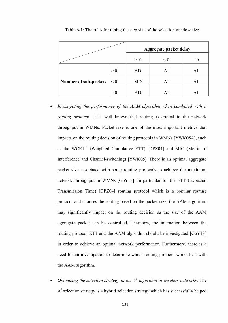
131
Table 6-1: The rules for tuning the step size of the selection window size
Investigating the performance of the AAM algorithm when combined with a
routing protocol. It is well known that routing is critical to the network
throughput in WMNs. Packet size is one of the most important metrics that
impacts on the routing decision of routing protocols in WMNs [YWK05A], such
as the WCETT (Weighted Cumulative ETT) [DPZ04] and MIC (Metric of
Interference and Channel-switching) [YWK05]. There is an optimal aggregate
packet size associated with some routing protocols to achieve the maximum
network throughput in WMNs [GoY13]. In particular for the ETT (Expected
Transmission Time) [DPZ04] routing protocol which is a popular routing
protocol and chooses the routing based on the packet size, the AAM algorithm
may significantly impact on the routing decision as the size of the AAM
aggregate packet can be controlled. Therefore, the interaction between the
routing protocol ETT and the AAM algorithm should be investigated [GoY13]
in order to achieve an optimal network performance. Furthermore, there is a
need for an investigation to determine which routing protocol works best with
the AAM algorithm.
Optimizing the selection strategy in the A3 algorithm in wireless networks. The
A3
selection strategy is a hybrid selection strategy which has successfully helped
Aggregate packet delay
> 0 < 0 = 0
Number of sub-packets
> 0 AD AI AI
< 0 MD AI AI
= 0 AD AI AI

132
to achieve the goal of the best aggregation trade-off in terms of realizing the
maximum average throughput with the minimum average delay. There may be
some other selection strategies that could be used to further improve the
throughput. For example, a priority strategy based on the least life time could be
used to reduce the delay by selecting the packets which have the smallest life
time [LYY09]. In particular, for the multi-hop wireless networks, the value
density selection strategy [Mod82] can be used where the packets are selected
based on the value density. The value density of a packet is defined as the
number of transmitted hop-counts per payload in byte. The largest value density
packet in the input buffer is serviced first in order to reduce the packet dropped.
Specifying the values of the target aggregate packet size and the maximum
acceptable delay parameters for different application types. Currently, the
values of the both parameters are fixed and specified by the user at the outset.
There may be further benefits in terms of network performance if these
parameters can be specified according to the application types. There is one
method that can be implemented in several steps. At first, all the applications
within a mixed traffic load are divided into two classes based on tagging and
packet size [EEV06], the time sensitive application (e.g. VoIP, video streaming)
and the time insensitive application (e.g. E-mail) which are pushed into separate
buffers. Here, the biggest drawback is that it may fail to identify the time
sensitive application packets as they tend not to use tagging. Then the values of
the two parameters for each class of application can be specified for the different
applications in order to improve the network performance. For example, for the
time sensitive applications the maximum acceptable delay and the target
aggregate packet size can be specified in order to minimize the delay. For the
133
time insensitive applications, the values of the two parameters can be specified
in order to maximize the throughput. After that, the two classes of applications
each employ separate AAM algorithms to aggregate packets based on the
different specified input parameters. Finally, the aggregate packets are moved
into the output buffer and are transmitted based on the arrival time. The
aggregate packet of the time sensitive application is moved into the output
buffer first if there are two aggregate packets arrivals into the output buffer at
the same time. Another method that can be used is to develop a smart algorithm
which can adaptively adjust the values of the two parameters based on the
different traffic loads. The values of the two parameters can be adaptively
adjusted based on the ratio of the small size packets to the overall packets which
arrive within a certain duration of time (e.g. 20 ms). The values of the two
parameters are inversely proportional to the value of this ratio. The reason for
this is that the VoIP packet is a small size packet and is time sensitive packet.
Here, the biggest challenge is that how to determine what constitutes a small
size packet and what time duration to use and how to adjust the values of the
two parameters based on the ratio in order to achieve the best network
performance.
134
6.3 Publications
The publications arising from this thesis are as followings:
[1] Jianhua Deng, Mark Davis, “An Adaptive Packet Aggregation Algorithm for
Wireless Networks,” International Conference on Wireless Communications and Signal
Processing 2013 (WCSP 2013), pp. 449-504, Hangzhou, China, 24 -26 October 2013.
[2] Jianhua Deng, Mark Davis, “The Performance of the Adaptive Aggregation
Mechanism (AAM) in Lossy Wireless Networks,” acceptable for publication at 20th
IEEE Symposium on Communications and Vehicular Technology in the Benelux 2013
(IEEE SCVT 2013), Namur, Belgium, 21 November 2013.

135
References
A
[AbA11] O. M. F. Abu-sharkh, M. J. Abdelhadi, “The Impact of Multi-Rate Operation
on A-MSDU, A-MPDU and Block Acknowledgment in Greenfield IEEE802.11n
wireless LANs,” IEEE Wireless Advanced (WiAd), pp. 116-121, London, UK, 20-22
June 2011.
[AbZ08] A. Abdrabou, W. Zhang , “Service Time Approximation in IEEE 802.11
Single-Hop Ad Hoc Networks”, IEEE Transactions on Wireless Communications, vol.
7, no. 1, pp. 305-313, January 2008.
[ACB11] P. H. Azevêdo, M. F. Caetano, J. L. Bordim, “A Packet Aggregation
Mechanism for Real Time Applications over Wireless Networks,” IEEE International
Symposium on Parallel and Distributed Processing Workshops and PhD Forum 2011,
pp. 648-655, Shanghai, China, 16-20 May 2011.
[AGS03] S. Ansari, R. S. G, and C. H.S, “Packet Sniffing: Brief Introduction,” IEEE
Potentials, vol. 21, pp. 17-19, December 2002.
[AhE10] S. S. Ahmeda, E. a. Esseid, “Review of routing metrics and protocols for
wireless mesh network,” Second Pacific-Asia Conference on Circuits, Communications
and System 2010, no. 1, pp. 27-30, Beijing, China, 1-2 August 2010.
[Any12] C. Anymore, “IEEE 802.11ac - Wi-Fi for the Mobile and Video Generation,”
2012 BROADCOM CORPORATION, pp. 1-6, January 2012. [Online]. Available at:
http://www.5gwifi.org/images/uploads/add/Wi-Fi-Primer100-R.pdf, [last accessed on 9
October 2013]
136
[ARC02] S. Ansari, S.G. Rajeev, H.S. Chandrashekar, “Packet sniffing: a brief
introduction”, IEEE Potentials, vol. 21, issue 5, pp. 17 – 19, December 2002 - January
2003.
[ArS12] T.Y. Arif, R.F. Sari, "An analytical model of A-MSDU scheme with
enhanced Block ACK for IEEE 802.11n networks", 2012 18th IEEE International
Conference on Networks (ICON), pp. 291 – 298, 12 – 14 December 2012.
[ath9] ath9k, 2013. [Online]: Available at
http://wireless.kernel.org/en/users/Drivers/ath9k, [last accessed on 29 January 2014]
[ath10] ath10k, 2013. [Online]: Available at
http://wireless.kernel.org/en/users/Drivers/ath10k, [last accessed on 29 January 2014]
B
[BaA12] G. Barreira, J. Ascenso, “Impact of the IEEE 802.11n Frame Aggregation
Mechanisms on Video Streaming Quality,” 20th
International Conference on Software,
Telecommunications and Computer Networks (SoftCOM), pp. 1-5, Split, Croatia, 11-13
September 2012.
[BBC10] J. L. Bordim, A. V. Barbosa, M. F. Caetano, P. S. Barreto, “IEEE802.11b/g
Standard: Theoretical Maximum Throughput,” First International Conference on
Networking and Computing 2010, pp. 197-201, Higashi-Hiroshima, Japan, 17-19
November 2010.
[BBE99] S. Bajaj, L. Breslau, D. Estrin, “Improving Simulation for Network Research”,
Technical Report 99-702, University of Southern California, 4 March, 1999. [Online].
Available at: http://ilab.cs.byu.edu/zappala/pubs/usc-cs-tr-99-702.pdf, [last accessed on
9 October 2013]

137
[BEF00] L. Breslau, D. Estrin, K. Fall, S. Floyd, J. Heidemann, a. Helmy, P. Huang, S.
McCanne, K. Varadhan, “Advances in network simulation,” Computer, vol. 33, pp. 59-
67, May 2000.
[BMS09] G. Bhanage, R. Mahindra, I. Seskar, D. Raychaudhuri, “Implication of MAC
Frame Aggregation on Empirical Wireless Experimentation,” IEEE Global
Telecommunications Conference 2009 (GLOBECOM 2009), pp. 1-7, Honolulu, HI,
USA, 30 November -4 December 2009.
C
[CDK07] M. Castro, P. Dely, J. Karlsson, A. Kassler, “Capacity increase for voice
over ip traffic through packet aggregation in wireless multihop mesh networks,” Future
Generation Communication and Networking (FGCN 2007), Jeju, South Korea, pp. 350
- 355, 6-8 December 2007.
[CiS00] S.Ci, H. Sharif, “Adaptive Approaches to Enhance Throughput of IEEE
802.11 Wireless LAN with Bursty Channel,” 25th
Annual IEEE Conference Local
Computer Networks, Tampa, Florida, USA, pp. 44-45, 8-10 November 2000.
[CIS13] CISCO, 2013. [Online]. Available at:
http://www.cisco.com/en/US/tech/tk722/tk809/tsd_technology_support_protocol_home.
html, [last accessed on 9 October 2013]
[CLC07] Y. Chang, C. Lee, and J. A. Copeland, “Dynamic Optimal Fragmentation for
Goodput Enhancement in IEEE 802.11 WLAN,” 3rd
International Conference on
Testbeds and Research Infrastructure for the Development of Networks and
Communities 2007 (TridentCom 2007), pp. 1-9, Lake Buena Vista, Florida, USA, 21-23
May 2007
D

138
[DAM11] Y. Daldoul, T. Ahmed, D. Meddour, “IEEE 802.11n Aggregation
Performance Study for the Multicast,” Wireless Days (WD), 2011 IFIP, pp. 4-9,
Niagara Falls, USA, 10-12 October 2011.
[DPZ04] R. Draves, J. Padhye, B. Zill, “Routing in Multi-Radio Multi-Hop Wireless
Mesh Networks,” Tenth Annual International Conference on Mobile Computing and
Networking 2004 (ACM MobiCom’04), Philadelphia, Pennsylvania, USA, 26 September
- 1 October 2004.
[DPZ04] R. Draves, J. Padhye, B. Zill, “Routing in Multi-Radio, Multi-Hop Wireless
Mesh Networks,” 10th
annual international conference on Mobile computing and
networking 2004 (ACM Mobicom 2004), Philadelphia, Pennsylvania, USA, 26
September - 1 October, 2004
E
[EEV06] M. Ergen, S. C. Ergen, P. Varaiya, “Throughput Performance of a Wireless
VoIP Model with Packet Aggregation in IEEE 802.11,” IEEE Wireless
Communications and Networking Conference 2006 (WCNC 2006), vol. 4, pp. 2235-
2239, Las Vegas, NV, USA, 3-6 April, 2006.
F
[Fra03] T. Franklin, “Wireless Local Area Networks in Education,” TechLearn
Technical Report, New York, 2003. [Online]. Available at:
http://www.jisc.ac.uk/media/documents/publications/wirelesslantechrep.pdf, [last
accessed on 9 October 2013]
G
139
[Gas05] M. S. Gast, “802.11 Wireless Networks: The Definitive Guide”, Second
Edition, published by O’Reilly Media, Inc., 2005. ISBN 978-0-596-10052-0
[GiK07] B. Ginzburg, A. Kesselman, “Performance Analysis of A-MPDU and A-
MSDU Aggregation in IEEE 802.11n,” IEEE Sarnoff Symposium, pp. 1-5, Nassau Inn,
Princeton, NJ, USA, 30 April -2 May 2007
[Gop03] R.A. Gopalakrishna, “Network Packet Aggregation,” U.S. Patent US 6614808
B1, Date of patent, 2 September 2003.
[GoY13] D. Gong, Y. Yang, “Distributed Algorithms for Joint Routing and Frame
Aggregation in 802.11n Wireless Mesh Networks,” IEEE 27th
International Symposium
on Parallel & Distributed Processing, pp. 1122-1132, Boston, MA, USA, 20-24 May
2013.
[GuL12] S. Gübner, C. Lindemann, “Evaluating the Impact of Frame Aggregation on
Video-Streaming over IEEE 802.11n multihop Networks,” IEEE World of Wireless,
Mobile and Multimedia Networks (WoWMoM), pp. 1-6, San Francisco, CA, USA, 25-
28 June 2012.
H
[HeC03] J. He, S. H. G. Chan, “TCP and UDP performance for Internet over optical
packet switched networks,” IEEE International Conference on Communications (ICC
'03), vol. 2, pp. 1350-1354, 11-15 May 2003.
[HLL08] X. He, F. Y. Li, J. Lin, “Link Adaptation with Combined Optimal Frame Size
and Rate Selection in Error-Prone 802.11n Networks,” IEEE International Symposium
on Wireless Communication Systems 2008 (ISWCS '08), pp. 733-737, Reykjavik,
Iceland, 21-24 October 2008.
140
[Hud09] T. M. N. Huda, “Throughput Enhancement of IEEE 802.11 WLAN for
Multimedia Communications,” First Asian Himalayas International Conference (AH-
ICI), pp. 1-6, Kathmandu, Nepal, 3-5 November 2009.
[PiH08] R. Pierre, F. Hoefel, “IEEE 802.11n MAC Improvements: A MAC and PHY
Cross-Layer Model to Estimate the Throughput,” IEEE 68th
Vehicular Technology
Conference 2008 (VTC 2008-Fall), pp. 1-5, Calgary, BC, Canada, 21-24 September
2008.
[HLF09] Y. Huang, J. Lin, K. Feng, “Performance Analysis for Aggregated Selective
Repeat ARQ Scheme in IEEE 802.11n Networks,” IEEE 20th
International Symposium
on Personal, Indoor and Mobile Radio Communications 2009, pp. 37-41, Tokyo, Japan,
13-16 September 2009.
I
[IEa99] IEEE Standard for Information technology — Telecommunications and
information exchange between systems — Local and metropolitan area networks —
Specific requirements — Part 11: Wireless LAN Medium Access Control (MAC) and
Physical Layer (PHY) specifications: High-speed Physical Layer in the 5 GHZ Band
(vol. 1999). [Online]. Available at:
http://ieeexplore.ieee.org/stamp/stamp.jsp?tp=&arnumber=815305, [last accessed on 9
October 2013]
[IEEb99] IEEE Standard for Information technology — Telecommunications and
information exchange between systems — Local and metropolitan area networks —
Specific requirements — Part 11: Wireless LAN Medium Access Control (MAC) and
Physical Layer (PHY) specifications: Higher-Speed Physical Layer Extension in the 2.4
GHz Band (vol. 1999). [Online]. Available at:

141
http://ieeexplore.ieee.org/stamp/stamp.jsp?tp=&arnumber=817038, [last accessed on 9
October 2013]
[IEE03] IEEE Standard for Information technology — Telecommunications and
information exchange between systems — Local and metropolitan area networks —
Specific requirements — Part 11: Wireless LAN Medium Access Control (MAC) and
Physical Layer (PHY) specifications Amendment 4: Further Higher Data Rate
Extension in the 2.4 GHz Band (vol. 2003). [Online]. Available at:
http://ieeexplore.ieee.org/stamp/stamp.jsp?tp=&arnumber=4014509, [last accessed on 9
October 2013]
[IEE05] IEEE Standard for Information technology - Telecommunications and
information exchange between systems - Local and metropolitan area networks -
Specific requirements-Part 15.1: Wireless Medium Access Control (MAC) and Physical
Layer (PHY) Specifications for Wireless Personal Area Networks (WPANs) (vol. 2005)
[Online]. Available at:
http://ieeexplore.ieee.org/stamp/stamp.jsp?tp=&arnumber=1490827, [last accessed on 9
October 2013]
[IEE09] IEEE Standard for Information technology —Local and metropolitan area
networks — Specific requirements — Part 11: Wireless LAN Medium Access Control
(MAC) and Physical Layer (PHY) specifications Amendment 5: Enhancements for
Higher Throughput (vol. 2008). [Online]. Available at:
http://ieeexplore.ieee.org/servlet/opac?punumber=4749842, [last accessed on 9 October
2013]
[IEE11] IEEE Draft Standard for Information Technology-Telecommunications and
information exchange between systems-Local and metropolitan area networks-Specific

142
requirements-Part 11: Wireless LAN Medium Access Control (MAC) and Physical
Layer (PHY) specifications-Amendment 10: Mesh Networking. (vol. 2011). [Online].
Available at: http://ieeexplore.ieee.org/servlet/opac?punumber=5741228, [last accessed
on 9 October 2013]
[IEE13] “IEEE P802.11ac/D 7.0”, Institute of Electrical and Electronic Engineers,
2013. [Online]. Available at: http://www.techstreet.com/ieee/products/vendor_id/4473,
[last accessed on 9 October 2013]
[IEE97] IEEE Standard for Information technology — Telecommunications and
information Local and metropolitan area networks — Part 11: Wireless LAN Medium
Access Control (MAC) and Physical Layer (PHY) Specifications (vol. 1999). [Online].
Available at: http://ieeexplore.ieee.org/servlet/opac?punumber=5258, [last accessed on
9 October 2013]
[IEn09] IEEE Standard for Information technology-- Local and metropolitan area
networks-- Specific requirements-- Part 11: Wireless LAN Medium Access Control
(MAC) and Physical Layer (PHY) Specifications Amendment 5: Enhancements for
Higher Throughput. (vol. 2009). [Online]. Available at:
http://ieeexplore.ieee.org/servlet/opac?punumber=5307291, [last accessed on 9 October
2013]
[IES09] IEEE Standard for Local and metropolitan area networks Part 16: Air Interface
for Broadband Wireless Access Systems Amendment 1: Multi-hop Relay Specification.
(vol. 2009). [Online]. Available at:
http://ieeexplore.ieee.org/servlet/opac?punumber=5167146, [last accessed on 9 October
2013]

143
[ITU03] ITU, standard, “ITU-T-G.114- One-way transmission time,” International
Telecommunication Union, May 2007. [Online]. Available at: http://www.itu.int/ITU-
T/recommendations/rec.aspx?rec=6254, [last accessed on 9 October 2013]
J
[JDB10] M. G. Jibukumar, R. Datta, P. K. Biswas. “New Packet Aggregation Schemes
for Multimedia Applications in WLAN,” IEEE Network Operations and Management
Symposium (NOMS), pp. 424-431, Osaka, Japan, 19-23 April 2010.
[JGN03] A. Jain, M. Gruteser, M. Neufeld, D. Grunwald, “Benefits of Packet
Aggregation in Ad-Hoc Wireless Network,” Technical Report CU-CS-960-03,
Department of Computer Science, University of Colorado, August 2003. [Online].
Available at:
http://citeseerx.ist.psu.edu/viewdoc/download?doi=10.1.1.86.6126&rep=rep1&type=pd
f, [last accessed on 9 October 2013]
K
[KCK11] M. Kim, C. Choi, A. R. U. Kljk, V. Q. Zh, S. D. Mrlqw, “Joint Rate and
Fragment Size Adaptation in IEEE 802.11n Wireless LANs,” IEEE Consumer
Communications and Networking Conference (CCNC), pp. 942-947, Las Vegas, NV,
USA, 9-12 January 2011.
[KFW03] B. S. Kim, Y. Fang, T. F. Wong, and Y. Kwon, “Dynamic fragmentation
scheme for rate-adaptive wireless LANs,” 14th
IEEE International Symposium
Proceedings on Personal, lndoor and Mobile Radio Communication 2003, vol. 3, pp.
2591-2595, Beijing, China, 7-10 September 2003.
[KGL06] K. Kim, S. Ganguly, R. Lzmailov, S. Hong “On packet aggregation
mechanisms for improving VoIP quality in mesh networks,” IEEE 63rd
Vehicular

144
Technology Conference 2006, (VTC 2006), pp. 891-895, Melbourne, Victoria, Australia,
7-10 May 2006.
[KHS08] B. S. Kim, H. Y. Hwang, D. K. Sung, “Effect of Frame Aggregation on the
Throughput Performance of IEEE 802.11n,” IEEE Wireless Communications and
Networking Conference 2008 (WCNC 2008), pp. 1740-1744, Las Vegas, NV, USA, 31
March -3 April 2008.
[KJL13] J. Kim, S. Jung, K. Lee, J. Kim, “Frame Aggregation Scheme based on Voice
Quality in VoIP Systems”, 2013 International Conference on Electronics, Information
and Communication (ICEIC 2013), pp. 15 - 16 , Bali, Indonesia , 30January - 2
February 2013.
[KML12] Y. Kim, E. Monroy, O. Lee, K. Park, S. Choi, “Adaptive Two-Level Frame
Aggregation in IEEE 802.11n WLAN,” 18th
Asia-Pacific Conference on
Communications (APCC), pp. 658-663, Jeju Island, South Korea, 15-17 October 2012.
[KoG03] O. Komolafe, R. Gardner, “Aggregation of VoIP Streams in a 3G Mobile
Network: A Teletraffic Perspective”, 5th
European Personal Mobile Communications
Conference (EPMCC), pp. 3-7, Glasgow, UK, 22-25 April 2003.
[KSP12] G. Kim, C. Shin, H. Park, “Adaptive frame size estimation using extended
Kalman filter for high-stressed WLANs,” IEEE 23rd
International Symposium on
Personal, Indoor and Mobile Radio Communications 2012 (PIMRC), pp. 272-277,
Sydney, Australia, 9-12 September 2012.
[KuD06] S. Kuppa, G. R. Dattatreya, “Modeling and Analysis of Frame Aggregation in
Unsaturated WLANs with Finite Buffer Stations,” IEEE International Conference on

145
Communications 2006 (ICC '06), vol. 3, pp. 967-972, Istanbul, Turkey, 11-15 June
2006.
L
[LCB10] I. Lopetegui, R.A. Carrasco, S. Boussakta, "VoIP design and implementation
with network coding schemes for wireless networks", 2010 7th International
Symposium on Communication Systems Networks and Digital Signal Processing
(CSNDSP), pp. 857 - 861, Newcastle upon Tyne, 21-23 July 2010.
[LeP07] S. Lee, S. Park, “Rotating Priority Queue based Scheduling Algorithm for
IEEE 802.11n WLAN,” 9th
International Conference on Advanced Communication
Technology, vol. 3, pp. 1702-1706, Gangwon-Do, South Korea, 12-14 February 2007.
[LeS98] P. Lettieri, M. B. Srivastava, “Adaptive frame length control for improving
wireless link throughput, range, and energy efficiency,” Seventeenth Annual Joint
Conference of the IEEE Computer and Communications Societies Gateway to the 21st
Century 1998 (IEEE INFOCOM’98), vol. 2, pp. 564-571, San Francisco, CA, USA, 29
March - 2 April 1998.
[LFH13] J. Lin, K. Feng, Y. Huang, Li-Chun Wang "Novel Design and Analysis of
Aggregated ARQ Protocols for IEEE 802.11n Networks", IEEE Transactions on
Mobile Computing, pp. 556 – 570, Vol. 12, Issue 3, March 2013.
[LHH05] Y. Li, J. Harnes, R. Holte, "Impact of Lossy Links on Performance of Multi-
hop Wireless Networks", IEEE 14th
International Conference on Computer
Communications and Networks 2005, pp. 303-308, San Diego, CA, USA, 17-19
October 2005.
[Lin06] Y. Lin, V. W.S. Wong, “Wsn01-1: Frame aggregation and optimal frame size
adaptation for IEEE 802.11n WLANs,” IEEE Global Telecommunications Conference
146
2006 (GLOBECOM ’06), pp. 1-6, San Francisco, CA, USA, 27 November - 1
December 2006.
[LMT04] M. Lacage, M. H. Manshaei, T. Turletti, and S. Antipolis, “IEEE 802.11 Rate
Adaptation: A Practical Approach,” 7th
ACM international symposium on Modeling,
analysis and simulation of wireless and mobile systems of 2004 (MSWiM'04), pp. 126-
134, Venezia, Italy, 4-6 October 2004.
[LNM09] T. Li, Q. Ni, D. Malone, D. Leith, Y. Xiao, “Aggregation with fragment
retransmission for very high-speed WLANs,” IEEE/ACM Transactions on Networking,
vol. 17, pp. 591-604, April 2009.
[LWM96] J. Liebeherr, D. E. Wrege, S. Member, and D. Ferrari, “Exact Admission
Control for Networks with a Bounded Delay Service,” IEEE/ACM Transactions on
Networking, vol. 4, pp. 885-901, December 1996.
[LYK08] K. Lee, S. Yun, H. Kim, “Boosting Video Capacity of IEEE 802.11n through
Multiple Receiver Frame Aggregation,” IEEE Vehicular Technology Conference 2008
(VTC Spring 2008), pp. 2587-2591, Singapore, 11-14 May 2008.
[LYY09] Y. Lin, J. Yeh, T. Yang, C. Ku, S. Tsao, and Y. Lai, “Efficient dynamic
frame aggregation in IEEE 802.11s mesh networks,” International Journal of
Communication Systems, pp. 1319-1338, June 2009.
M
[MaA12] A. Majeed, N. B. Abu-Ghazaleh, “Packet aggregation in multi-rate wireless
LANs,” 9th
Annual IEEE Communications Society Conference on Sensor, Mesh and Ad
Hoc Communications and Networks (SECON), pp. 452-460, Seoul, South Korea, 18-21
June 2012.

147
[MaE07] S. Maaroufi and H. Elbiaze, “Performance Evaluation of New MAC
Mechanisms for IEEE 802.11n,” Global Information Infrastructure Symposium 2007
(GIIS 2007), pp. 39-45, Marrakech, Morocco, 26 July 2007.
[MAH12] E. Makkiya, E.H. Al-Hemiary, "Impact of video transcoding profiles in
wireless multicast streaming", 2012 International Conference on Future
Communication Networks (ICFCN), pp. 111 – 116, Baghdad, 2-5 April 2012.
[MAG09] M. Malekzadeh, A. Azim, A. Ghani, J. Desa, S. Subramaniam, “Empirical
Analysis of Virtual Carrier Sense Flooding Attacks Over Wireless Local Area Network,”
Journal of Computer Science, vol. 5, no. 3, pp. 214-220, March 2009.
[MaS11] K. Marwah, G. Singh “VoIP over WMN: Effect of packet aggregation”,
International Journal on Computer Science and Engineering (IJCSE), pp. 2323 – 2331,
Vol. 3, 6 June 2011
[MBR12] B. Maqhat, M. D. Baba, R. A. Rahman, “A-MSDU Real Time Traffic
Scheduler for IEEE 802.11n WLANs,” IEEE Symposium on Wireless Technology and
Applications 2012 (ISWTA), pp. 286-290, Bandung, Indonesia, 23-26 September 2012
[Mod82] E. J. Moder, “The knapsack problem,” Journal of Parabola, vol. 18, pp. 6-
12, 1982.
[Mol11] A. F. Molisch, “wireless communication,” pp.128-130, First Edition, John
Wiley & Sons Ltd, United Kingdom, 2011. ISBN 0-47084888-X
N
[NGI03] V. Naoumov, T. Gross, D. Informatik, “Simulation of Large Ad Hoc
Networks,” the Sixth ACM International Workshop on Modeling, Analysis and

148
Simulation of Wireless and Mobile Systems 2003 (MSWiM 2003), San Diego, California,
USA, 19 September, 2003.
[NS212] ns-2, 2012. [Online]. Available at: http://www.isi.edu/nsnam/, [last accessed
on 9 October 2013]
[NS312] ns-3, 2012. [Online]. Available at:
http://www.nsnam.org/docs/release/3.18/tutorial/ns-3-tutorial.pdf, [last accessed on 9
October 2013]
[NS313] ns-3, 2013. [Online]. Available at: http://www.nsnam.org/overview/key-
technologies/, [last accessed on 9 October 2013]
[NsP12] ns-3 project, 2012, “ns-3 Manual - Release 3.14,” [Online]. Available at:
http://www2.nsnam.org/docs/release/3.14/manual/html/organization.html, [last
accessed on 9 October 2013]
O
[OPN12] OPNET Technology, 2012. [Online]. Available: http://www.opnet.com/,
[last accessed on 9 October 2013]
Q
[QCS02] D. Qiao, S. Choi, K. G. Shin, “Goodput Analysis and Link Adaptation for
IEEE 802.11a Wireless LANs,” IEEE Transaction on Mobile Computing (TMC), vol. 1,
Issue 4, pp. 278-292, October-December 2002.
[QiC01] D. Qiao, S. Choi “Goodput Enhancement of IEEE 802.1l a Wireless LAN via
Link Adaptation,” IEEE International Conference on Communications 2001 (ICC
2001), vol. 7, pp. 1995-2000, Helsinki, Finland, 11-14 June 2001.
149
[QIZ10] M. A. Qadeer, A. Iqbal, M. Zahid, M. R. Siddiqui, “Network Traffic Analysis
and Intrusion Detection Using Packet Sniffer,” Second International Conference on
Communication Software and Networks 2010 (ICCSN’10), pp. 313-317, Singapore, 26-
28 February 2010.
R
[R&S11] Rohde&Schwarz, “IEEE 802.11n/IEEE 802.11 ac digital standards for signal
generators Operating Manual,” pp. 10-12, 2011. [Online]. Available at:
http://www.rohde-schwarz.de/file/RS_SigGen_IEEE80211_Operating_en_15.pdf, [last
accessed on 9 October 2013]
[Rap02] T. S. Rappaport. “Wireless Communications, Principles and Practice”, second
edition, Prentice Hall, pp. 66, 2002. ISBN-10: 0130422320
[RLI06] T. Razafindralambo, I. G. Lassous, L. Iannone, S. Fdida, “Dynamic packet
aggregation to solve performance anomaly in 802.11 wireless networks,” 9th
ACM
international symposium on Modeling analysis and simulation of wireless and mobile
systems 2006 (MSWiM '06), pp. 247-254, Torremolinos, Spain, 2-6 October 2006.
[RMP08] R. Riggio, D. Miorandi, F. De. Pellegrini, F. Granelli, “A traffic aggregation
and differentiation scheme for enhanced QoS in IEEE 802.11-based wireless mesh
networks,” Computer Communications, vol. 31, Issue 7, pp. 1290-1300, May 2008.
[RoD01] Roddy, Dennis, “Satellite Communications”, pp. 89, third edition, McGraw-
Hill, 2001. ISBN 0070077851
S
[SaA12] M. Samih, E. Al-Hemiary, “Impact of TCP Congestion Control Algorithms on
IEEE802.11n MAC Frame Aggregation”, International Journal of Computer Science
Engineering and Technology (IJCSET), pp. 1410 – 1414, vol. 2, September 2012.

150
[SeS10] T. Selvam, S. Srikanth, “A Frame Aggregation Scheduler for IEEE 802.11n,”
National Conference on Communications 2010 (NCC’10), pp. 1-5, Chennai, India, 29-
31 January 2010.
[SHW10] P. Sedtheetorn, K. Hamdi, L. Wuttisittikuljit, “Accurate packet error rate
analysis of variable spreading gain-code division multiaccess and multicode-code
division multiaccess wireless communication networks”, IET Communications, Vol.
5 , Issue 16, pp. 2407 – 2417, November 2011.
[SNC08] D. Skordoulis, Q. Ni, H. H. Chen, A. P. Stephens, C. Liu, A. Jamalipour,
“IEEE 802.11n MAC frame aggregation mechanisms for next-generation high-
throughput WLANs,” IEEE Wireless Communications, vol. 5, Issue 1, pp. 40-47,
February 2008.
[SOA11] M. Seyedzadegan, M. Othman, B. M. Ali, S. Subramaniam, “Wireless Mesh
Networks: WMN Overview, WMN Architecture,” International Conference on
Communication Engineering and Networks 2011 (IPCSIT), vol. 19, pp. 12-18, Hong
Kong, China, 25-27 November 2011
[SOS10] A. Saif, M. Othman, S. Subramaniam, N. Abdulhamid, “Impact of
aggregation headers on aggregating small MSDUs in 802.11n WLANs,” International
Conference on Computer Applications and Industrial Electronics 2010 (ICCAIE’10), pp.
630-635, Kuala Lumpur, Malaysian, 5-8 December 2010.
[SOS11] A. Saif, M. Othman, S. Subramaniam, N. A. W. A. Hamid, “An Enhanced
A-MSDU Frame Aggregation Scheme for 802.11n Wireless Networks,” Wireless
Personal Communications, vol. 66, no. 4, pp. 683-706, June 2011.
151
[SWC99] S. Shaffer, D. Weiss J. Casuba, “Method for constructing and adaptive
packet lengths in a congested network,” U.S. Patent US 6003089, Filed Mar.31, 1997,
Date of patent, 14 December 1999.
[SWS10] D. Shen, X. Wang, Y. Sun, N. Bao, M. Wu, L. Shen, “The performance of
adaptive frame aggregation with delay limits in ultrahigh-speed WLAN,” IEEE 12th
International Conference on Communication Technology 2010, pp. 1364-1368, Nanjing,
China, 11-14 November 2010.
[SYC06] A. Sidelnikov, J. Yu, S. Choi, “Fragmentation / Aggregation Scheme for
Throughput Enhancement of IEEE 802.11n WLAN,” 3rd
IEEE VTS Asia Pacific
Wireless Communications Symposium 2006 (APWCS 2006), pp. 37-39, Daejon, Korea,
24-25 August 2006.
T
[TeY13] P. Teymoori, N. Yazdani, “Delay-Constrained Optimized Packet Aggregation
in High-Speed Wireless Networks,” Journal of Computer Science and Technology, vol.
28, pp. 525-539, May 2013.
[ThW12] Wireshark, 2012. [Online]: https://www.wireshark.org/, [last accessed on 9
October 2013]
[Tim13] Timeline of IEEE 802.11 ac, 2013. [Online]. Available at:
http://grouper.ieee.org/groups/802/11/Reports/802.11_Timelines.htm, [last accessed on
9 October 2013]
[TNS12] The Network Simulator, 2012. [Online]. Available at:
http://www.nsnam.org/overview/publications, [last accessed on 9 October 2013]

152
[TYH10] P. Teymoori, N. Yazdani, S. A. Hoseini, “Analyzing Delay Limits of High-
Speed Wireless Ad hoc Networks Based on IEEE 802.11n,” 5th
International
Symposium on Telecommunications 2010 (IST 2010), pp. 489-495, Tehran, Iran, 4-6
December 2010.
W
[WaH08] F. Wang, M. Hamdi, “A Scheduler for the Downlink of Multi-user Wire-
less Systems with Frame Aggregation,” Global Telecommunications Conference 2008
(IEEE GLOBECOM 2008), pp. 1-5, New Orleans, LO, USA, 30 November - 4
December 2008.
[War12] L. Ward, “802.11ac technology Introduction White Paper,” BROADCOM
CORPORATION, pp. 92, 2012. [Online]. Available at:
http://www.5gwifi.org/images/uploads/add/Wi-Fi-Primer100-R.pdf, [last accessed on 9
October 2013]
[WeL11] W. Wen, D. Liu, “An adaptive retry scheme for delay-constrained service
transmission in 802.11n system,” International Conference on Computational Problem-
Solving 2011 (ICCP), pp. 97-101, Chengdu, China, 21-23 October 2011.
[Wik13] wikipedia, 2013. [Online]. Available at:
http://en.wikipedia.org/wiki/IEEE_802.11ac-cite_note-timelines-1/, [last accessed on 9
October 2013]
[Wir13] Wireshark version 1.8.6, 2013. [Online]. Available at:
http://www.wireshark.org/, [last accessed on 9 October 2013]
[Wla12] P. Teymoori, A. Dadlani, K. Sohraby, K. Kim, “An Optimal Packet Aggregation
Scheme in Delay-Constrained IEEE 802.11n WLANs,” 8th
International Conference on

153
Wireless Communications, Networking and Mobile Computing 2012 (WiCOM 2012),
pp. 1-4, Shanghai, China, 21-23 September 2012.
X
[Xia04] Y.Xiao, “Packing Mechanisms for the IEEE 802.11n Wireless LANs,” IEEE
Global Telecommunications Conference 2004 (GLOBECOM '04), pp. 3275-3279, vol. 5,
29 November - 3 December 2004.
[Xia05] Y.Xiao. “IEEE 802.11n: Enhancements for higher throughput in wireless
LANs,” IEEE Wireless Communications, vol. 12, Issue 6, pp. 82-91, December 2005.
[XiR02] Y.Xiao, J. Rosdahl, “Throughput and Delay Limits of IEEE 802.11,” IEEE
Communications Letters, vol. 6, Issue 8, pp. 355-357, August 2002.
[XiR03] Y.Xiao, J. Rosdahl, “Performance analysis and enhancement for the current
and future IEEE 802.11 MAC protocols,” ACM SIGMOBILE Mobile Computing
Communications Review, vol. 7, Issue 2, pp. 6-19, April 2003.
Y
[YCJ04] K. Youngsoo, S. Choi, K. Jang, “Throughput enhancement of IEEE 802.11
WLAN via frame aggregation,” IEEE 60th
Vehicular Technology Conference 2004
(VTC2004), vol. 4, pp. 3030-3034, 26-29 September 2004.
[YCL08] W. Yoon, S. Chung, S. Lee, and Y. Lee, “An efficient cooperation of on-
demand and proactive modes in Hybrid Wireless Mesh Protocol,” 33rd
IEEE
Conference on Local Computer Networks 2008 (LCN 2008), pp. 52-57, 14-17 October
2008.
[YLF09] Y. Huang, J. Lin, K. Feng “Performance Analysis for Aggregated Selective
Repeat ARQ Scheme in IEEE 802.11n Networks,” IEEE 20th
International Symposium
154
on Personal, Indoor and Mobile Radio Communications 2009, pp. 37-41, Tokyo, Japan,
13-16 September 2009.
[YWA04] J. Yin, X. Wang, D. P. Agrawal, “Optimal Packet Size in Error-prone
Channel for IEEE 802.11Distributed Coordination Function,” IEEE Wireless
Communications and Networking Conference 2004 (WCNC 2004). vol. 3, pp. 1654-
1659, Atlanta, Georgia, USA, 21-25 March 2004.
[YWK05A] Y. Yang, J. Wang, R. Kravets, “Designing Routing Metrics for Mesh
Networks,” IEEE Workshop on Wireless Mesh Networks 2005, pp. 1-5, Santa Clara, CA,
USA, 26 September 2005.
[YWK05] Y. Yang, J. Wang, R. Kravets, “Interference-aware Load Balancing for
Multi-hop Wireless Networks,” Tech. Report UIUCDCS-R-2005-2526, Department of
Computer Science, University of Illinois at Urbana-Champaign, October 2005. [Online].
Available at: https://www.ideals.illinois.edu/bitstream/handle/2142/10974/Interference-
aware%20Load%20Balancing%20for%20Multihop%20Wireless%20Networks.pdf?seq
uence=2, [last accessed on 9 October 2013]
Z
[ZaL13] B.W. Zarikoff, D.J. Leith, "Measuring Pulsed Interference in 802.11
Links", IEEE/ACM Transactions on Networking, pp. 509 - 521 Vol. 21, Issue 2, April
2013.
[ZCY10] H. Zheng, G. Chen, and L. Yu, “Video Transmission over IEEE 802.11n
WLAN with Adaptive Aggregation Scheme,” IEEE International Symposium on
Broadband Multimedia Systems and Broadcasting 2010 (BMSB), pp. 1-5, Shanghai,
China, 24-26 March 2010.
155
[ZeX03] Y. R. Zheng C. Xiao, “ Simulation Models with Correct Statistical
Properties for Rayleigh Fading Channels,” IEEE Transactions on Communications,
vol. 51, no. 6, pp. 920-928, June 2003.
[ZhN08] F. Zheng and J. Nelson, “Adaptive Design for the Packet Length of IEEE
802.11n Networks,” IEEE International Conference on Communications 2008 (ICC
'08), pp. 2490-2495, Beijing, China, 19-23 May 2008.
[ZIF08] Q. Zhang, V. B. Iversen, F. H. P. Fitzek, “Throughput and Delay Performance
Analysis of Packet Aggregation Scheme for PRMA,” IEEE Wireless Communications
and Networking Conference 2008 (WCNC 2008), pp. 1380-1384, Las Vegas, NV, USA,
31 March - 3 April 2008.
[ZKH13] W. Zhang, K. Kwak, L. Hou, “Frame aggregation scheme based on dynamic
pricing”, Communications, China, vol.10, Issue 10, pp. 115 – 124, October 2013.
[ZNN10] B. Zhang, T. S. E. Ng, A. Nandi, R. Riedi, P. Druschel, G. Wang,
“Measurement based analysis, modeling, and synthesis of the internet delay space,”
IEEE/ACM Transactions on Networking, vol. 18, Issue 1, pp. 229-242, February 2010.
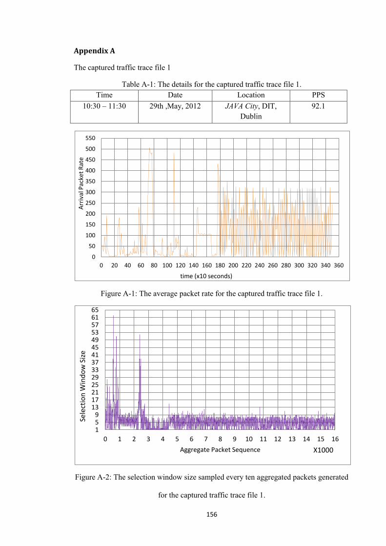
156
Appendix A
The captured traffic trace file 1
Table A-1: The details for the captured traffic trace file 1.
Time Date Location PPS
10:30 – 11:30 29th ,May, 2012 JAVA City, DIT,
Dublin
92.1
Figure A-1: The average packet rate for the captured traffic trace file 1.
Figure A-2: The selection window size sampled every ten aggregated packets generated
for the captured traffic trace file 1.
0
50
100
150
200
250
300
350
400
450
500
550
0 20 40 60 80 100 120 140 160 180 200 220 240 260 280 300 320 340 360
Arr
ival
Pac
ket
Rat
e
time (x10 seconds)
1 5 9
13 17 21 25 29 33 37 41 45 49 53 57 61 65
0 1 2 3 4 5 6 7 8 9 10 11 12 13 14 15 16
Sele
ctio
n W
ind
ow
Siz
e
Aggregate Packet Sequence X1000

157
The captured traffic trace file 2
Table A-2: The details for the captured traffic trace file 2.
Time Date Location PPS
12:00 – 13:00 29th ,May, 2012 JAVA City, DIT,
Dublin
114
Figure A-3: The average packet rate for the captured traffic trace file 2.
Figure A-4: The selection window size sampled every ten aggregated packets generated
for the captured traffic trace file 2.
0
50
100
150
200
250
300
350
400
450
0 20 40 60 80 100 120 140 160 180 200 220 240 260 280 300 320 340 360
Arr
ival
Pac
ket
Rat
e
time (x10 seconds)

158
The captured traffic trace file 3
Table A-3: The details for the captured traffic trace file 3.
Time Date Location PPS
14:00 – 15:00 29th ,May, 2012 JAVA City, DIT,
Dublin
75.7
Figure A-5: The average packet rate for the captured traffic trace file 3.
Figure A-6: The selection window size sampled every ten aggregated packets generated
for the captured traffic trace file 3.
0
50
100
150
200
250
300
350
400
450
0 20 40 60 80 100 120 140 160 180 200 220 240 260 280 300 320 340 360
Arr
ival
Pac
ket
Rat
e
time (x10 seconds)
1
3
5
7
9
11
13
15
17
19
21
23
25
0 1 2 3 4 5 6 7 8 9 10 11 12
Slec
eti
on
Win
do
w S
ize
Aggregate Packet Sequence x1000
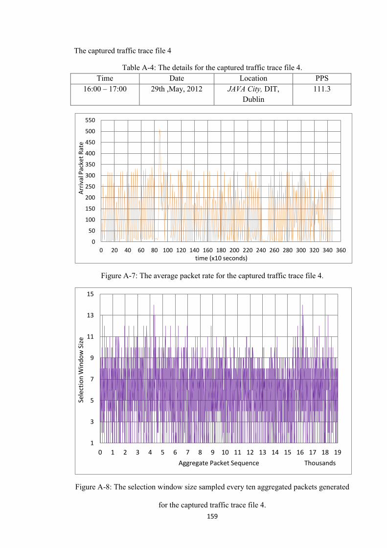
159
The captured traffic trace file 4
Table A-4: The details for the captured traffic trace file 4.
Time Date Location PPS
16:00 – 17:00 29th ,May, 2012 JAVA City, DIT,
Dublin
111.3
Figure A-7: The average packet rate for the captured traffic trace file 4.
Figure A-8: The selection window size sampled every ten aggregated packets generated
for the captured traffic trace file 4.
0
50
100
150
200
250
300
350
400
450
500
550
0 20 40 60 80 100 120 140 160 180 200 220 240 260 280 300 320 340 360
Arr
ival
Pac
ket
Rat
e
time (x10 seconds)
1
3
5
7
9
11
13
15
0 1 2 3 4 5 6 7 8 9 10 11 12 13 14 15 16 17 18 19
Sele
ctio
n W
ind
ow
Siz
e
Aggregate Packet Sequence Thousands

160
The captured traffic trace file 5
Table A-5: The details for the captured traffic trace file 5.
Time Date Location PPS
17:30 – 18:30 29th ,May, 2012 JAVA City, DIT,
Dublin
109.4
Figure A-9: The average packet rate for the captured traffic trace file 5.
Figure A-10: The selection window size sampled every ten aggregated packets
generated for the captured traffic trace file 5.
0
50
100
150
200
250
300
350
400
450
500
0 20 40 60 80 100 120 140 160 180 200 220 240 260 280 300 320 340 360
Arr
ival
Pac
ket
Rat
e
time (x10 seconds)
1
3
5
7
9
11
13
15
17
19
0 1 2 3 4 5 6 7 8 9 10 11 12 13 14 15 16 17 18 19 20
Sele
ctio
n W
ind
ow
Siz
e
Aggregate Packet Sequence X1000

161
The captured traffic trace file 6
Table A-6: The details for the captured traffic trace file 6
Time Date Location PPS
09:30 – 10:30 19th, June, 2012 Costa coffee shop, Dublin 9.4
Figure A-11: The average packet rate for the captured traffic trace file 6.
Figure A-12: The selection window size generated by the AAM algorithm for the
captured traffic trace file 6.
0 10 20 30 40 50 60 70 80 90
100 110 120 130 140 150 160 170 180
0 20 40 60 80 100 120 140 160 180 200 220 240 260 280 300 320
Arr
ival
Pac
ket
Rat
e
time (x10 seconds)
1
3
5
7
9
11
13
15
17
19
21
23
25
27
29
31
0 5 10 15 20 25 30 35 40 45 50 55 60 65 70 75 80 85
Sele
ctio
n W
ind
ow
Siz
e
Aggregate packet Sequence x 100

162
The captured traffic trace file 7
Table A-7: The details for the captured traffic trace file 7
Time Date Location PPS
11:00 –12:00 19th, June, 2012 Parliament Square, TCD,
Dublin
5.6
Figure A-13: The average packet rate for the captured traffic trace file 7.
Figure A-14: The selection window size generated by the AAM algorithm for the
captured traffic trace file 7.
0
5
10
15
20
25
30
35
40
45
50
0 20 40 60 80 100 120 140 160 180 200 220 240 260 280 300 320 340 360
Arr
ival
Pac
ket
Rat
e
time (x10 seconds)
1
2
3
4
5
6
7
8
9
10
11
12
0 3 6 9 12 15 18 21 24 27 30 33 36 39 42 45
Sele
ctio
n W
ind
ow
Siz
e
aggregate Packet Sequence x 100
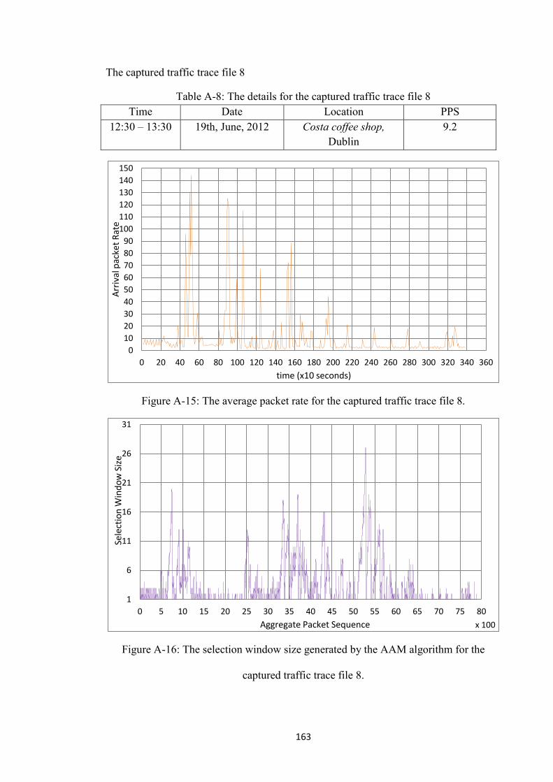
163
The captured traffic trace file 8
Table A-8: The details for the captured traffic trace file 8
Time Date Location PPS
12:30 – 13:30 19th, June, 2012 Costa coffee shop,
Dublin
9.2
Figure A-15: The average packet rate for the captured traffic trace file 8.
Figure A-16: The selection window size generated by the AAM algorithm for the
captured traffic trace file 8.
0
10
20
30
40
50
60
70
80
90
100
110
120
130
140
150
0 20 40 60 80 100 120 140 160 180 200 220 240 260 280 300 320 340 360
Arr
ival
pac
ket
Rat
e
time (x10 seconds)
1
6
11
16
21
26
31
0 5 10 15 20 25 30 35 40 45 50 55 60 65 70 75 80
Sele
ctio
n W
ind
ow
Siz
e
Aggregate Packet Sequence x 100
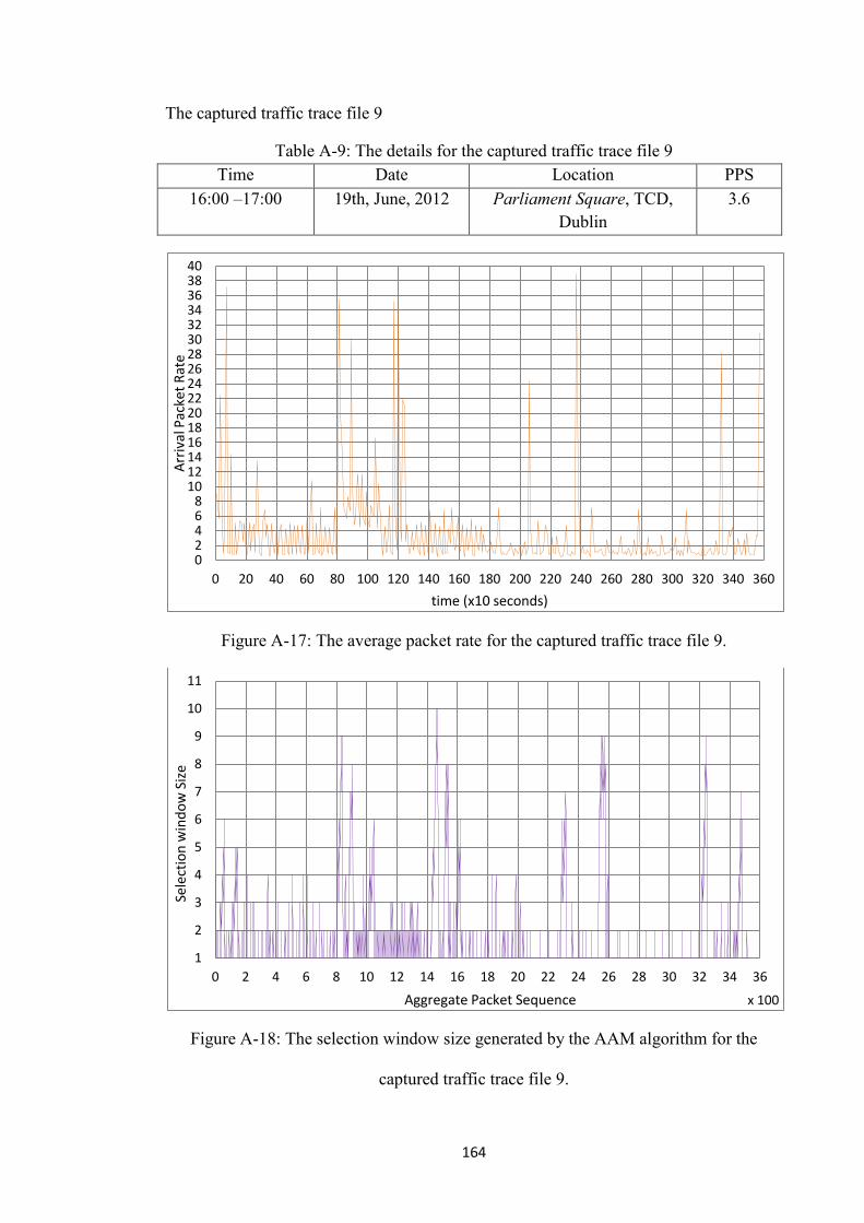
164
The captured traffic trace file 9
Table A-9: The details for the captured traffic trace file 9
Time Date Location PPS
16:00 –17:00 19th, June, 2012 Parliament Square, TCD,
Dublin
3.6
Figure A-17: The average packet rate for the captured traffic trace file 9.
Figure A-18: The selection window size generated by the AAM algorithm for the
captured traffic trace file 9.
0 2 4 6 8
10 12 14 16 18 20 22 24 26 28 30 32 34 36 38 40
0 20 40 60 80 100 120 140 160 180 200 220 240 260 280 300 320 340 360
Arr
ival
Pac
ket
Rat
e
time (x10 seconds)
1
2
3
4
5
6
7
8
9
10
11
0 2 4 6 8 10 12 14 16 18 20 22 24 26 28 30 32 34 36
Sele
ctio
n w
ind
ow
Siz
e
Aggregate Packet Sequence x 100

165
The captured traffic trace file 10
Table A-10: The details for the captured traffic trace file 10
Time Date Location PPS
17:00 – 18:00 19th, June, 2012 Costa coffee shop,
Dublin
6.6
Figure A-19: The average packet rate for the captured traffic trace file 10.
Figure A-20: The selection window size generated by the AAM algorithm for the
captured traffic trace file 10.
0
10
20
30
40
50
60
70
80
90
100
110
120
130
0 20 40 60 80 100 120 140 160 180 200 220 240 260 280 300 320 340
Arr
ival
Pac
ket
Rat
e
time (x10 seconds)
1 2 3 4 5 6 7 8 9
10 11 12 13 14 15 16 17 18 19 20
0 3 6 9 12 15 18 21 24 27 30 33 36 39 42 45 48 51 54 57 60 63
Slec
tio
n W
ino
dw
Siz
e
Aggregate Packet Sequence x 100
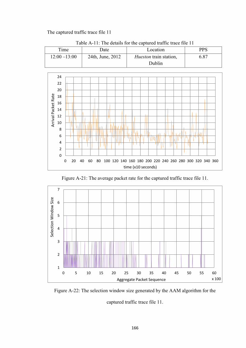
166
The captured traffic trace file 11
Table A-11: The details for the captured traffic trace file 11
Time Date Location PPS
12:00 –13:00 24th, June, 2012 Hueston train station,
Dublin
6.87
Figure A-21: The average packet rate for the captured traffic trace file 11.
Figure A-22: The selection window size generated by the AAM algorithm for the
captured traffic trace file 11.
0
2
4
6
8
10
12
14
16
18
20
22
24
0 20 40 60 80 100 120 140 160 180 200 220 240 260 280 300 320 340 360
Arr
ival
Pac
ket
Rat
e
time (x10 seconds)
1
2
3
4
5
6
7
0 5 10 15 20 25 30 35 40 45 50 55 60
Sele
ctio
n W
ind
ow
Siz
e
Aggregate Packet Sequence x 100

167
The captured traffic trace file 12
Table A-12: The details for the captured traffic trace file 12
Time Date Location PPS
13:30 – 14:30 24th, June, 2012 Hueston train station,
Dublin
4.2
Figure A-23: The average packet rate for the captured traffic trace file 12.
Figure A-24: The selection window size generated by the AAM algorithm for the
captured traffic trace file 12.
0
2
4
6
8
10
12
14
16
18
20
22
24
26
28
0 20 40 60 80 100 120 140 160 180 200 220 240 260 280 300 320 340 360
Arr
ival
pac
ket
Rat
e
time (x10 seconds)
1
2
3
4
5
6
0 2 4 6 8 10 12 14 16 18 20 22 24 26 28 30 32 34 36 38 40 42
Sele
ctio
n W
ind
ow
Siz
e
Aggregate Packet Sequence x 100
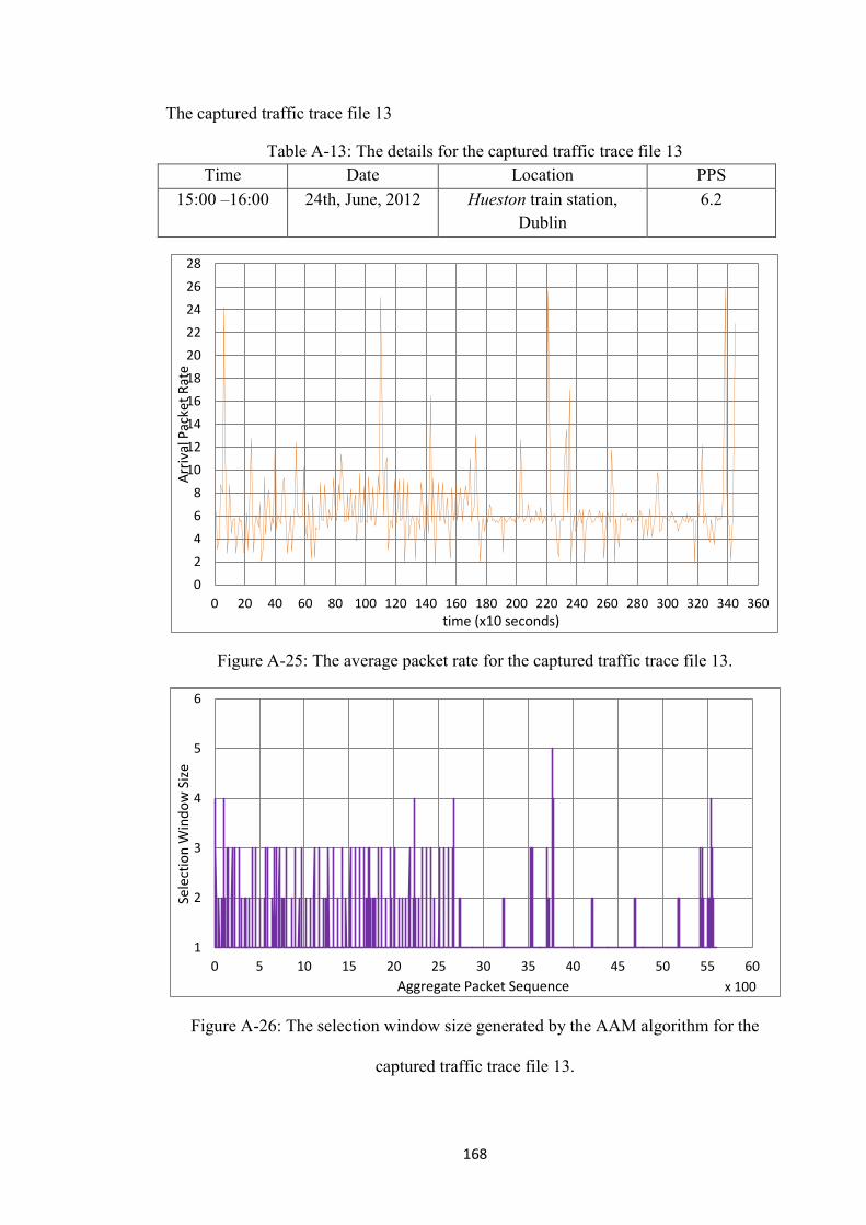
168
The captured traffic trace file 13
Table A-13: The details for the captured traffic trace file 13
Time Date Location PPS
15:00 –16:00 24th, June, 2012 Hueston train station,
Dublin
6.2
Figure A-25: The average packet rate for the captured traffic trace file 13.
Figure A-26: The selection window size generated by the AAM algorithm for the
captured traffic trace file 13.
0
2
4
6
8
10
12
14
16
18
20
22
24
26
28
0 20 40 60 80 100 120 140 160 180 200 220 240 260 280 300 320 340 360
Arr
ival
Pac
ket
Rat
e
time (x10 seconds)
1
2
3
4
5
6
0 5 10 15 20 25 30 35 40 45 50 55 60
Sele
ctio
n W
ind
ow
Siz
e
Aggregate Packet Sequence x 100

169
The captured traffic trace file 14
Table A-14: The details for the captured traffic trace file 14
Time Date Location PPS
10:30 –11:30 26th, June, 2012 Library, Kevin street, DIT,
Dublin
19.2
Figure A-27: The average packet rate for the captured traffic trace file 14.
Figure A-28: The selection window size generated by the AAM algorithm for the
captured traffic trace file 14.
0
20
40
60
80
100
120
140
160
180
200
220
240
260
280
300
320
0 20 40 60 80 100 120 140 160 180 200 220 240 260 280 300 320 340 360
Arr
ival
Pac
ketR
ate
time (x10 seconds)
1
6
11
16
21
26
31
36
0 1 2 3 4 5 6 7 8 9 10 11 12 13 14 15 16 17 18 19 20 21 22 23 24 25
Sele
ctio
n W
ind
ow
Siz
e
Aggregate Packet Sequence x 1000
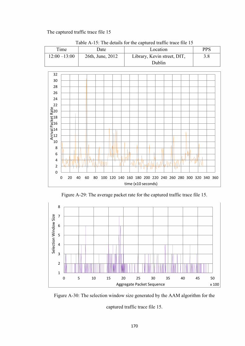
170
The captured traffic trace file 15
Table A-15: The details for the captured traffic trace file 15
Time Date Location PPS
12:00 –13:00 26th, June, 2012 Library, Kevin street, DIT,
Dublin
3.8
Figure A-29: The average packet rate for the captured traffic trace file 15.
Figure A-30: The selection window size generated by the AAM algorithm for the
captured traffic trace file 15.
0
2
4
6
8
10
12
14
16
18
20
22
24
26
28
30
32
0 20 40 60 80 100 120 140 160 180 200 220 240 260 280 300 320 340 360
Arr
ival
Pac
ket
Rat
e
time (x10 seconds)
1
2
3
4
5
6
7
8
0 5 10 15 20 25 30 35 40 45 50
Sele
ctio
n W
ind
ow
Siz
e
Aggregate Packet Sequence x 100
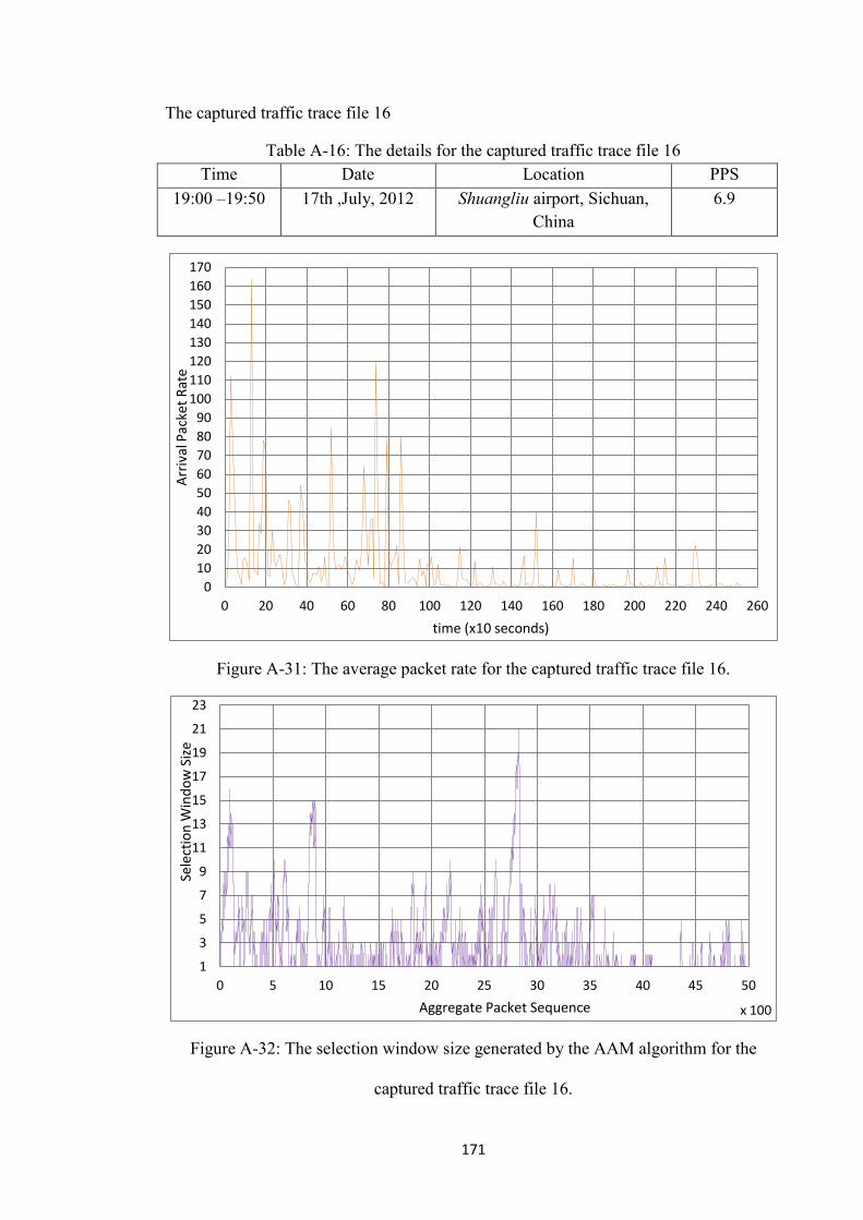
171
The captured traffic trace file 16
Table A-16: The details for the captured traffic trace file 16
Time Date Location PPS
19:00 –19:50 17th ,July, 2012 Shuangliu airport, Sichuan,
China
6.9
Figure A-31: The average packet rate for the captured traffic trace file 16.
Figure A-32: The selection window size generated by the AAM algorithm for the
captured traffic trace file 16.
0
10
20
30
40
50
60
70
80
90
100
110
120
130
140
150
160
170
0 20 40 60 80 100 120 140 160 180 200 220 240 260
Arr
ival
Pac
ket
Rat
e
time (x10 seconds)
1
3
5
7
9
11
13
15
17
19
21
23
0 5 10 15 20 25 30 35 40 45 50
Sele
ctio
n W
ind
ow
Siz
e
Aggregate Packet Sequence x 100

172
Appendix B
The captured traffic trace file 1
Table B-1: The details for the captured traffic trace file 1
Time Date Location PPS
10:30 – 11:30 29th ,May, 2012 JAVA City, DIT, Dublin 92.1
Figure B-1: The CCDF of the number of sub-packets for the captured traffic trace file 1.
0%
10%
20%
30%
40%
50%
60%
70%
80%
90%
100%
1 2 3 4 5 6 7 8 9 10 11 12 13 14 15 16 17 18 19 20 21 22 23 24 25 26 27 28
CC
DF
Number of sub-packets
FIFO SSFS AAM Fixed AAM with N=3 Fixed AAM with N=8 Fixed AAM with N=10
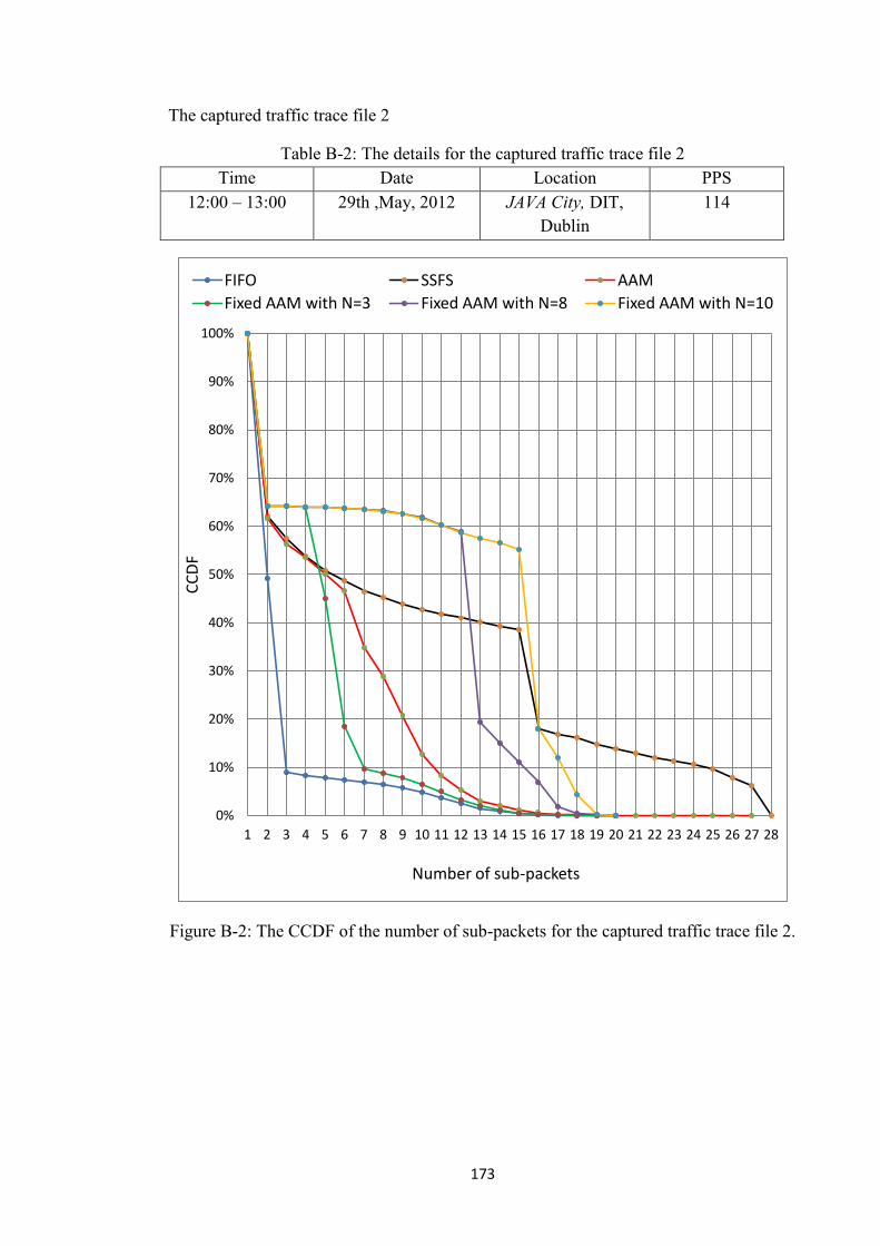
173
The captured traffic trace file 2
Table B-2: The details for the captured traffic trace file 2
Time Date Location PPS
12:00 – 13:00 29th ,May, 2012 JAVA City, DIT,
Dublin
114
Figure B-2: The CCDF of the number of sub-packets for the captured traffic trace file 2.
0%
10%
20%
30%
40%
50%
60%
70%
80%
90%
100%
1 2 3 4 5 6 7 8 9 10 11 12 13 14 15 16 17 18 19 20 21 22 23 24 25 26 27 28
CC
DF
Number of sub-packets
FIFO SSFS AAM
Fixed AAM with N=3 Fixed AAM with N=8 Fixed AAM with N=10

174
The captured traffic trace file 3
Table B-3: The details for the captured traffic trace file 3
Time Date Location PPS
14:00 – 15:00 29th ,May, 2012 JAVA City, DIT,
Dublin
75.7
Figure B-3: The CCDF of the number of sub-packets for the captured traffic trace file 3.
0%
10%
20%
30%
40%
50%
60%
70%
80%
90%
100%
1 2 3 4 5 6 7 8 9 10 11 12 13 14 15 16 17 18 19 20 21 22 23 24 25 26 27 28
CC
DF
Number of sub-packets
FIFO SSFS AAM
Fixed AAM with N=3 Fixed AAM with N=8 Fixed AAM with N=10

175
The captured traffic trace file 4
Table B-4: The details for the captured traffic trace file 4
Time Date Location PPS
16:00 – 17:00 29th ,May, 2012 JAVA City, DIT,
Dublin
111.3
Figure B-4: The CCDF of the number of sub-packets for the captured traffic trace file 4.
0%
10%
20%
30%
40%
50%
60%
70%
80%
90%
100%
1 2 3 4 5 6 7 8 9 10 11 12 13 14 15 16 17 18 19 20 21 22 23 24 25 26 27 28
CC
DF
Number of sub-packets
FIFO SSFS AAM
Fixed AAM with N=3 Fixed AAM with N=8 Fixed AAM with N=10

176
The captured traffic trace file 5
Table B-5: The details for the captured traffic trace file 5
Time Date Location PPS
17:30 – 18:30 29th ,May, 2012 JAVA City, DIT,
Dublin
109.4
Figure B-5: The CCDF of the number of sub-packets for the captured traffic trace file 5.
0%
10%
20%
30%
40%
50%
60%
70%
80%
90%
100%
1 2 3 4 5 6 7 8 9 10 11 12 13 14 15 16 17 18 19 20 21 22 23 24 25 26 27 28
CC
DF
Number of sub-packets
FIFO SSFS AAM
Fixed AAM with N=3 Fixed AAM with N=8 Fixed AAM with N=10

177
The captured traffic trace file 6
Table B-6: The details for the captured traffic trace file 6
Time Date Location PPS
09:30 – 10:30 19th, June, 2012 Costa coffee shop, Dublin 9.4
Figure B-6: The CCDF of the number of sub-packets for the captured traffic trace file 6.
0%
10%
20%
30%
40%
50%
60%
70%
80%
90%
100%
1 2 3 4 5 6 7 8 9 10 11 12 13 14 15 16 17 18 19 20 21 22 23 24 25 26 27 28
CC
DF
number of sub-packets
FIFO SSFS AAM
Fixed AAM with N=3 Fixed AAMwith N=8 Fixed AAM with N=10

178
The captured traffic trace file 7
Table B-7: The details for the captured traffic trace file 7
Time Date Location PPS
11:00 –12:00 19th, June, 2012 Parliament Square, TCD,
Dublin
5.6
Figure B-7: The CCDF of the number of sub-packets for the captured traffic trace file 7.
0%
10%
20%
30%
40%
50%
60%
70%
80%
90%
100%
1 2 3 4 5 6 7 8 9 10 11 12 13 14 15 16 17 18 19 20 21 22 23 24 25 26 27 28
CC
DF
Number of sub-packets
FIFO SSFS AAM
Fixed AAM with N=3 Fixed AAM with N=8 Fixed AAM with N=10

179
The captured traffic trace file 8
Table B-8: The details for the captured traffic trace file 8
Time Date Location PPS
12:30 – 13:30 19th, June, 2012 Costa coffee shop,
Dublin
9.2
Figure B-8: The CCDF of the number of sub-packets for the captured traffic trace file 8.
0%
10%
20%
30%
40%
50%
60%
70%
80%
90%
100%
1 2 3 4 5 6 7 8 9 10 11 12 13 14 15 16 17 18 19 20 21 22 23 24 25 26 27 28
CC
DF
Number of sub-packets
FIFO SSFS AAM
Fixed AAM with N=3 Fixed AAM with N=8 Fixed AAM with N=10

180
The captured traffic trace file 9
Table B-9: The details for the captured traffic trace file 9
Time Date Location PPS
16:00 –17:00 19th, June, 2012 Parliament Square, TCD,
Dublin
3.6
Figure B-9: The CCDF of the number of sub-packets for the captured traffic trace file 9.
0%
10%
20%
30%
40%
50%
60%
70%
80%
90%
100%
1 2 3 4 5 6 7 8 9 10 11 12 13 14 15 16 17 18 19 20 21 22 23 24 25 26 27 28
CC
DF
Number of sub-packets
FIFO SSFS AAM
Fixed AAM with N=3 Fixed AAMwith N=8 Fixed AAM with N=10
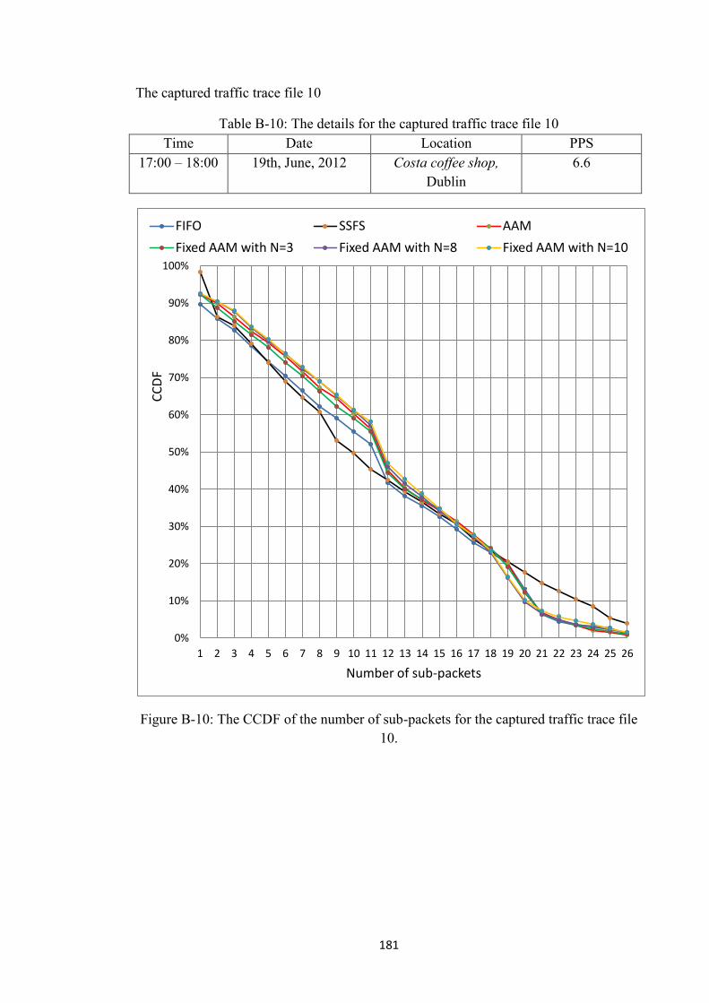
181
The captured traffic trace file 10
Table B-10: The details for the captured traffic trace file 10
Time Date Location PPS
17:00 – 18:00 19th, June, 2012 Costa coffee shop,
Dublin
6.6
Figure B-10: The CCDF of the number of sub-packets for the captured traffic trace file
10.
0%
10%
20%
30%
40%
50%
60%
70%
80%
90%
100%
1 2 3 4 5 6 7 8 9 10 11 12 13 14 15 16 17 18 19 20 21 22 23 24 25 26
CC
DF
Number of sub-packets
FIFO SSFS AAM
Fixed AAM with N=3 Fixed AAM with N=8 Fixed AAM with N=10

182
The captured traffic trace file 11
Table B-11: The details for the captured traffic trace file 11
Time Date Location PPS
12:00 –13:00 24th, June, 2012 Hueston train station,
Dublin
6.87
Figure B-11: The CCDF of the number of sub-packets for the captured traffic trace file
11.
0%
10%
20%
30%
40%
50%
60%
70%
80%
90%
100%
0 1 2 3 4 5 6 7 8 9 10 11 12 13 14 15 16 17 18 19 20 21 22 23 24 25
CC
DF
Number of sub-packets
FIFO AAM SSFS
Fixed AAM with N=3 Fixed AAM with N=8 Fixed AAM with N=10

183
The captured traffic trace file 12
Table B-12: The details for the captured traffic trace file 12
Time Date Location PPS
13:30 – 14:30 24th, June, 2012 Hueston train station,
Dublin
4.2
Figure B-12: The CCDF of the number of sub-packets for the captured traffic trace file
12.
0%
10%
20%
30%
40%
50%
60%
70%
80%
90%
100%
1 2 3 4 5 6 7 8 9 10 11 12 13 14 15 16 17 18 19 20 21 22 23 24 25
CC
DF
Number of sub-packets
FIFO AAM SSFS
Fixed AAM with N=3 Fixed AAM with N=8 Fixed AAM with N=10
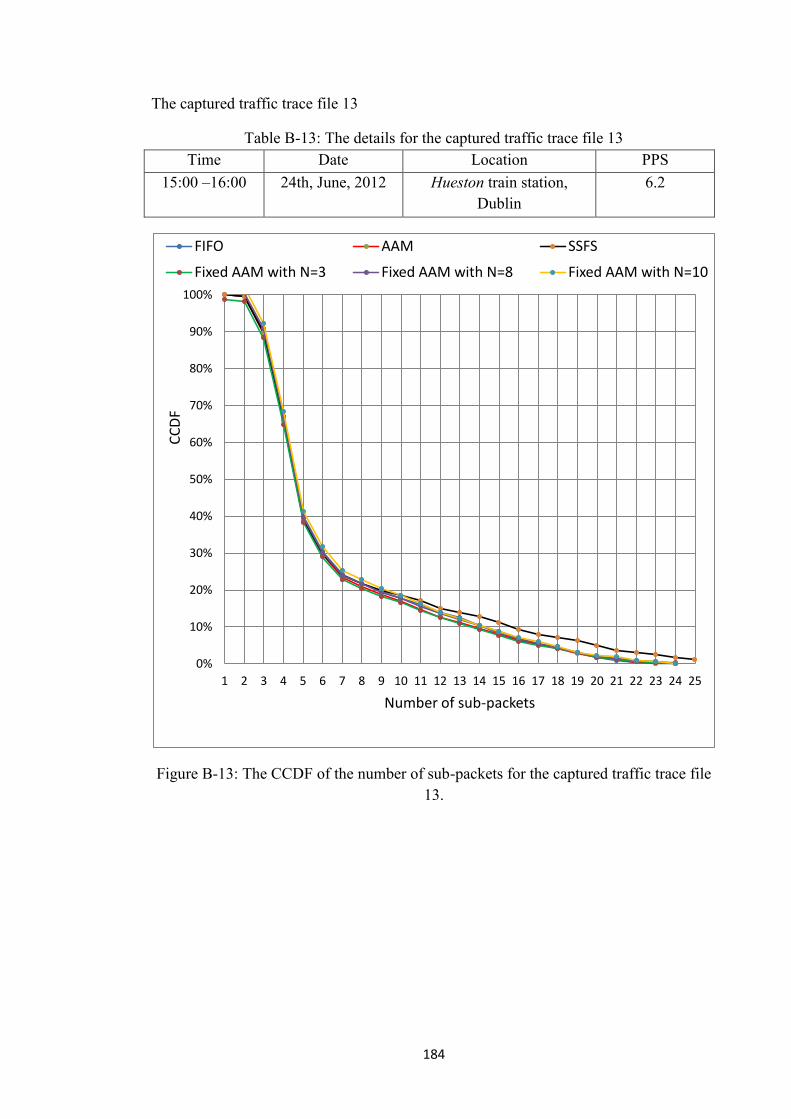
184
The captured traffic trace file 13
Table B-13: The details for the captured traffic trace file 13
Time Date Location PPS
15:00 –16:00 24th, June, 2012 Hueston train station,
Dublin
6.2
Figure B-13: The CCDF of the number of sub-packets for the captured traffic trace file
13.
0%
10%
20%
30%
40%
50%
60%
70%
80%
90%
100%
1 2 3 4 5 6 7 8 9 10 11 12 13 14 15 16 17 18 19 20 21 22 23 24 25
CC
DF
Number of sub-packets
FIFO AAM SSFS
Fixed AAM with N=3 Fixed AAM with N=8 Fixed AAM with N=10

185
The captured traffic trace file 14
Table B-14: The details for the captured traffic trace file 14
Time Date Location PPS
10:30 –11:30 26th, June, 2012 Library, Kevin street, DIT,
Dublin
19.2
Figure B-14: The CCDF of the number of sub-packets for the captured traffic trace file
14.
0%
10%
20%
30%
40%
50%
60%
70%
80%
90%
100%
1 2 3 4 5 6 7 8 9 10 11 12 13 14 15 16 17 18 19 20 21 22 23 24 25 26 27 28 29
CC
DF
Number of Sub-packets
FIFO SSFS AAM
Fixed AAM with N=3 Fixed AAM with N=8 Fixed AAM with N=10

186
The captured traffic trace file 15
Table B-15: The details for the captured traffic trace file 15
Time Date Location PPS
12:00 –13:00 26th, June, 2012 Library, Kevin street, DIT,
Dublin
3.8
Figure B-15: The CCDF of the number of sub-packets for the captured traffic trace file
15.
0%
10%
20%
30%
40%
50%
60%
70%
80%
90%
100%
1 2 3 4 5 6 7 8 9 10 11 12 13 14 15 16 17 18 19 20
CC
DF
Number of sub-packets
FIFO SSFS AAM
Fixed AAM with N=3 Fixed AAMwith N=8 Fixed AAM with N=10
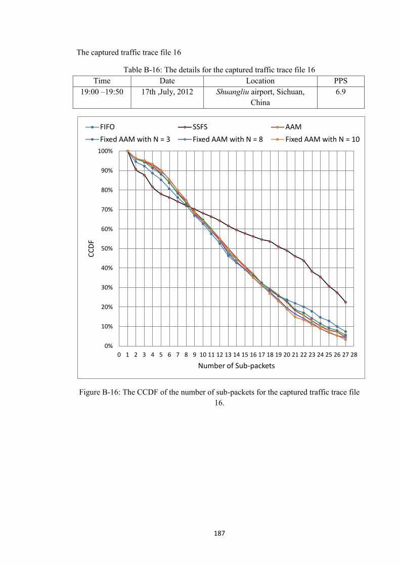
187
The captured traffic trace file 16
Table B-16: The details for the captured traffic trace file 16
Time Date Location PPS
19:00 –19:50 17th ,July, 2012 Shuangliu airport, Sichuan,
China
6.9
Figure B-16: The CCDF of the number of sub-packets for the captured traffic trace file
16.
0%
10%
20%
30%
40%
50%
60%
70%
80%
90%
100%
0 1 2 3 4 5 6 7 8 9 10 11 12 13 14 15 16 17 18 19 20 21 22 23 24 25 26 27 28
CC
DF
Number of Sub-packets
FIFO SSFS AAM
Fixed AAM with N = 3 Fixed AAM with N = 8 Fixed AAM with N = 10
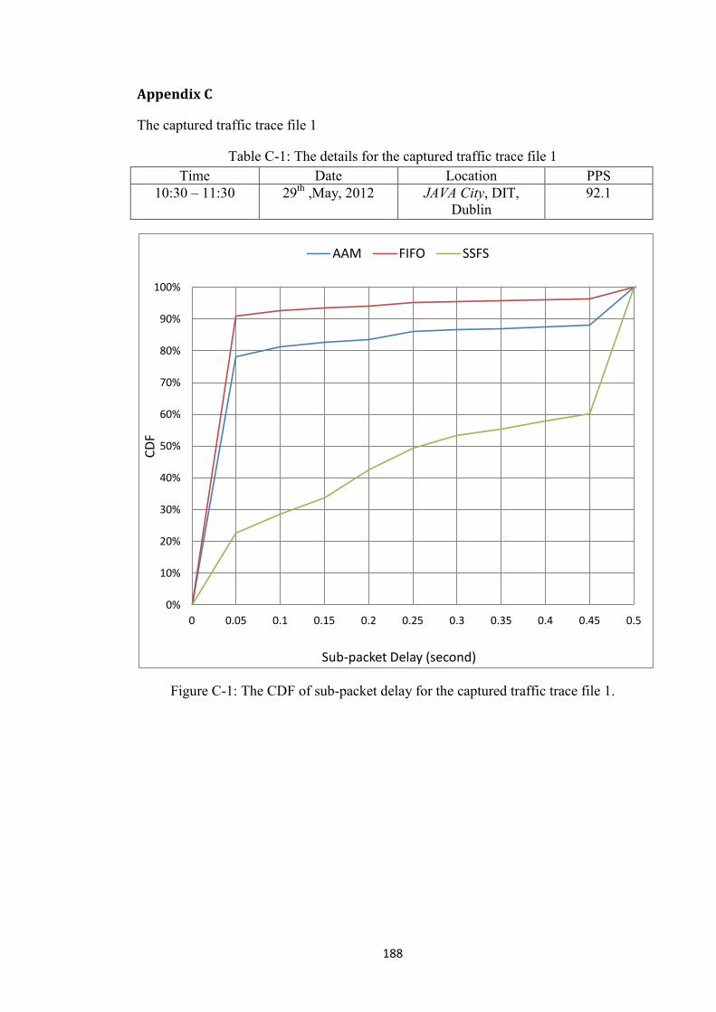
188
Appendix C
The captured traffic trace file 1
Table C-1: The details for the captured traffic trace file 1
Time Date Location PPS
10:30 – 11:30 29th
,May, 2012 JAVA City, DIT,
Dublin
92.1
Figure C-1: The CDF of sub-packet delay for the captured traffic trace file 1.
0%
10%
20%
30%
40%
50%
60%
70%
80%
90%
100%
0 0.05 0.1 0.15 0.2 0.25 0.3 0.35 0.4 0.45 0.5
CD
F
Sub-packet Delay (second)
AAM FIFO SSFS
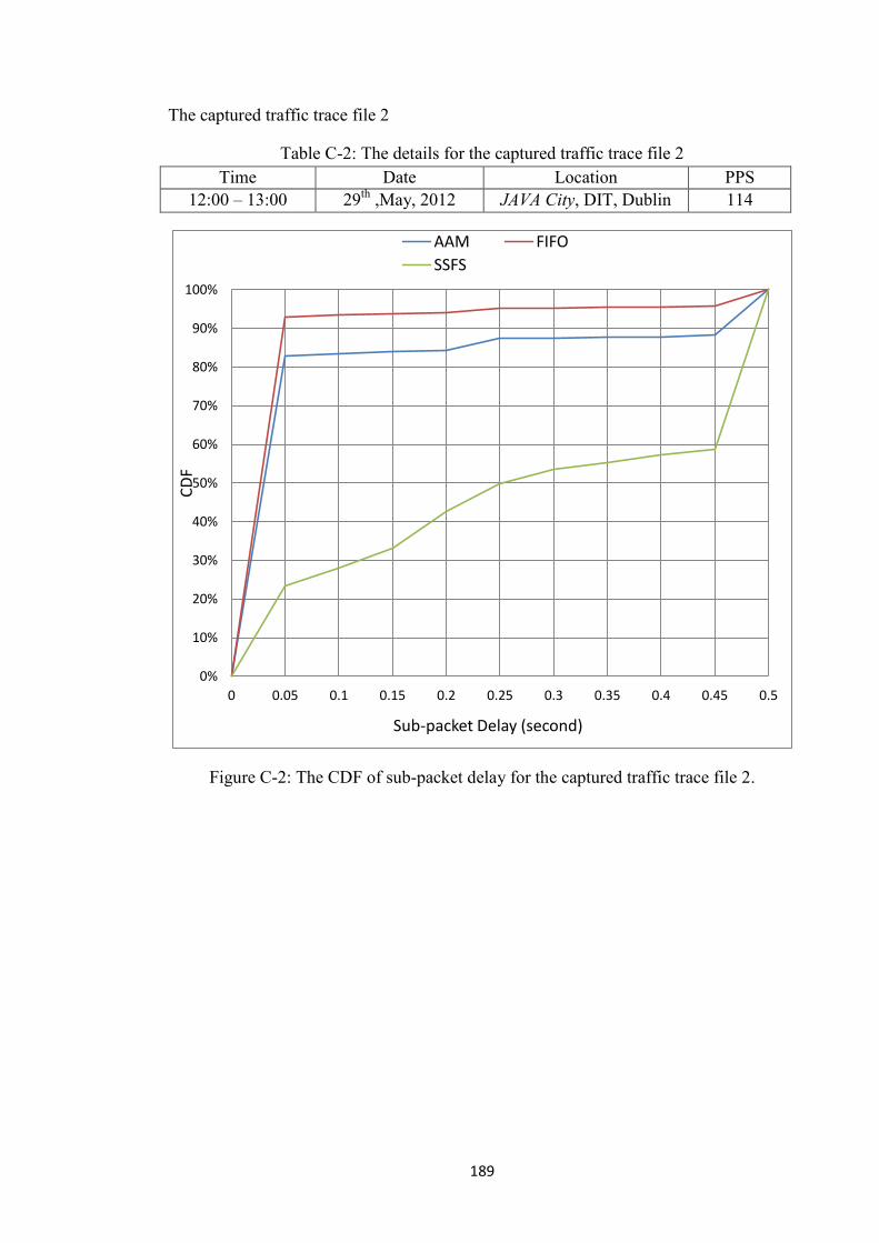
189
The captured traffic trace file 2
Table C-2: The details for the captured traffic trace file 2
Time Date Location PPS
12:00 – 13:00 29th
,May, 2012 JAVA City, DIT, Dublin 114
Figure C-2: The CDF of sub-packet delay for the captured traffic trace file 2.
0%
10%
20%
30%
40%
50%
60%
70%
80%
90%
100%
0 0.05 0.1 0.15 0.2 0.25 0.3 0.35 0.4 0.45 0.5
CD
F
Sub-packet Delay (second)
AAM FIFO
SSFS
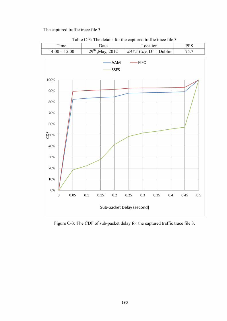
190
The captured traffic trace file 3
Table C-3: The details for the captured traffic trace file 3
Time Date Location PPS
14:00 – 15:00 29th
,May, 2012 JAVA City, DIT, Dublin 75.7
Figure C-3: The CDF of sub-packet delay for the captured traffic trace file 3.
0%
10%
20%
30%
40%
50%
60%
70%
80%
90%
100%
0 0.05 0.1 0.15 0.2 0.25 0.3 0.35 0.4 0.45 0.5
CD
F
Sub-packet Delay (second)
AAM FIFO
SSFS
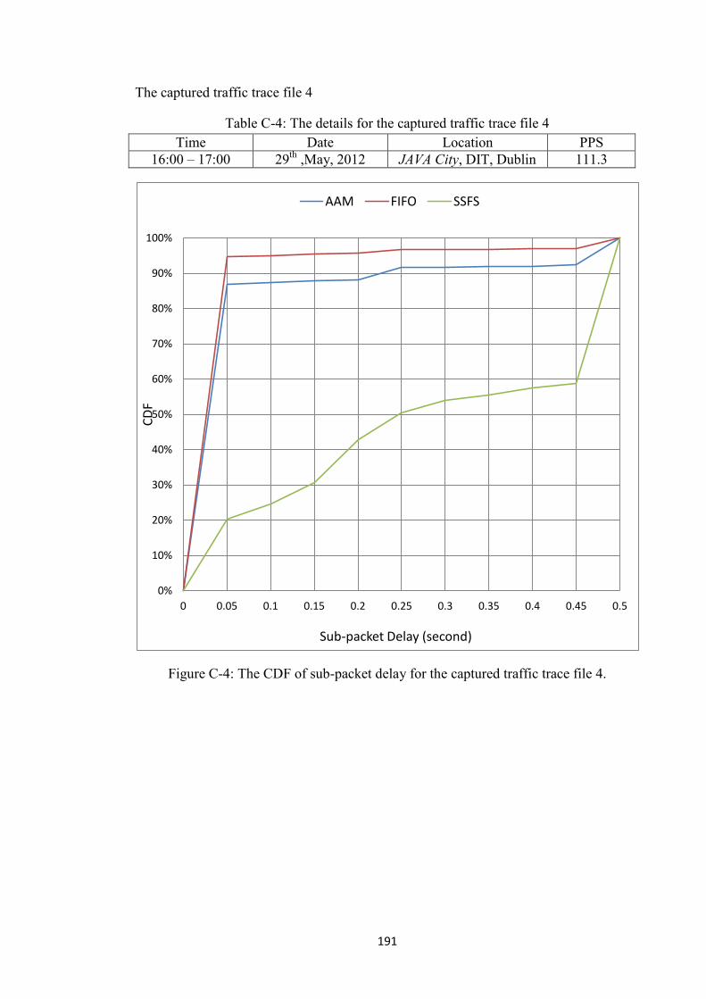
191
The captured traffic trace file 4
Table C-4: The details for the captured traffic trace file 4
Time Date Location PPS
16:00 – 17:00 29th
,May, 2012 JAVA City, DIT, Dublin 111.3
Figure C-4: The CDF of sub-packet delay for the captured traffic trace file 4.
0%
10%
20%
30%
40%
50%
60%
70%
80%
90%
100%
0 0.05 0.1 0.15 0.2 0.25 0.3 0.35 0.4 0.45 0.5
CD
F
Sub-packet Delay (second)
AAM FIFO SSFS
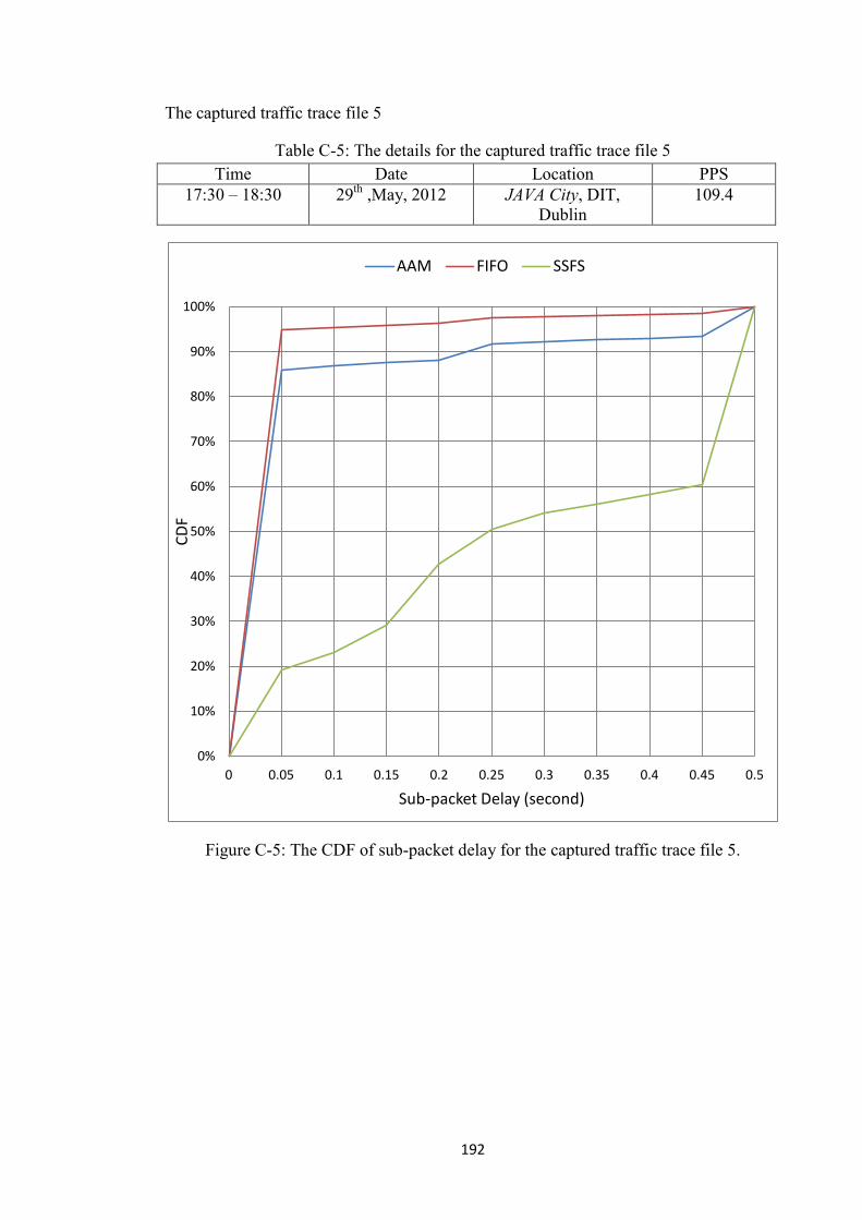
192
The captured traffic trace file 5
Table C-5: The details for the captured traffic trace file 5
Time Date Location PPS
17:30 – 18:30 29th
,May, 2012 JAVA City, DIT,
Dublin
109.4
Figure C-5: The CDF of sub-packet delay for the captured traffic trace file 5.
0%
10%
20%
30%
40%
50%
60%
70%
80%
90%
100%
0 0.05 0.1 0.15 0.2 0.25 0.3 0.35 0.4 0.45 0.5
CD
F
Sub-packet Delay (second)
AAM FIFO SSFS
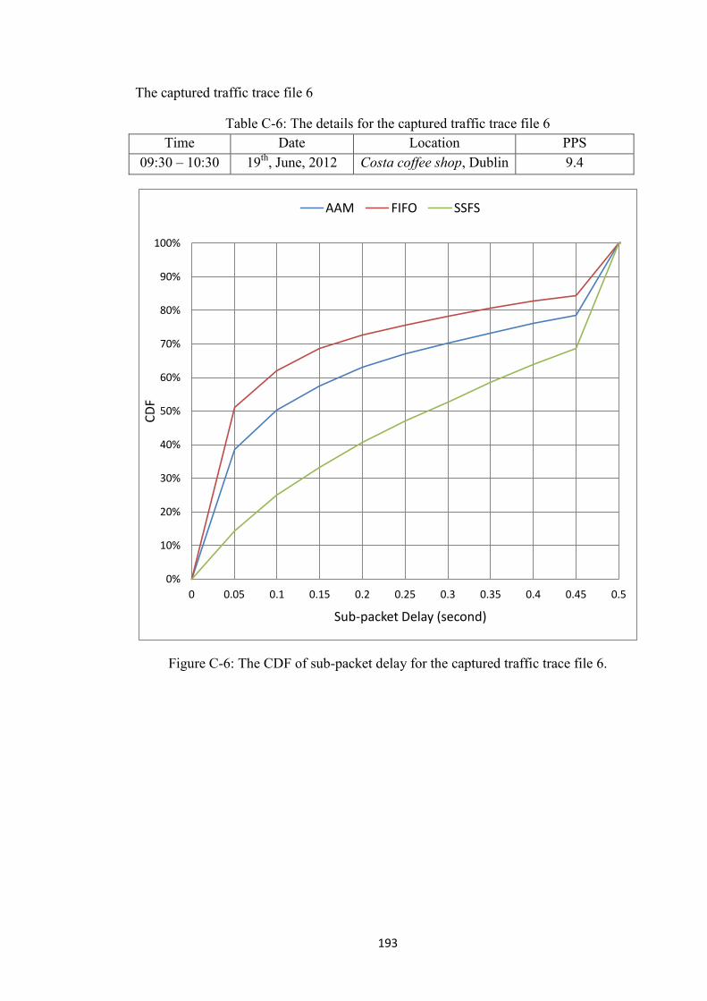
193
The captured traffic trace file 6
Table C-6: The details for the captured traffic trace file 6
Time Date Location PPS
09:30 – 10:30 19th
, June, 2012 Costa coffee shop, Dublin 9.4
Figure C-6: The CDF of sub-packet delay for the captured traffic trace file 6.
0%
10%
20%
30%
40%
50%
60%
70%
80%
90%
100%
0 0.05 0.1 0.15 0.2 0.25 0.3 0.35 0.4 0.45 0.5
CD
F
Sub-packet Delay (second)
AAM FIFO SSFS

194
The captured traffic trace file 7
Table C-7: The details for the captured traffic trace file 7
Time Date Location PPS
11:00 –12:00 19th
, June, 2012 Parliament Square, TCD,
Dublin
5.6
Figure C-7: The CDF of sub-packet delay for the captured traffic trace file 7.
0%
10%
20%
30%
40%
50%
60%
70%
80%
90%
100%
0 0.05 0.1 0.15 0.2 0.25 0.3 0.35 0.4 0.45 0.5
CD
F
Sub-packet Delay (second)
AAM FIFO SSFS
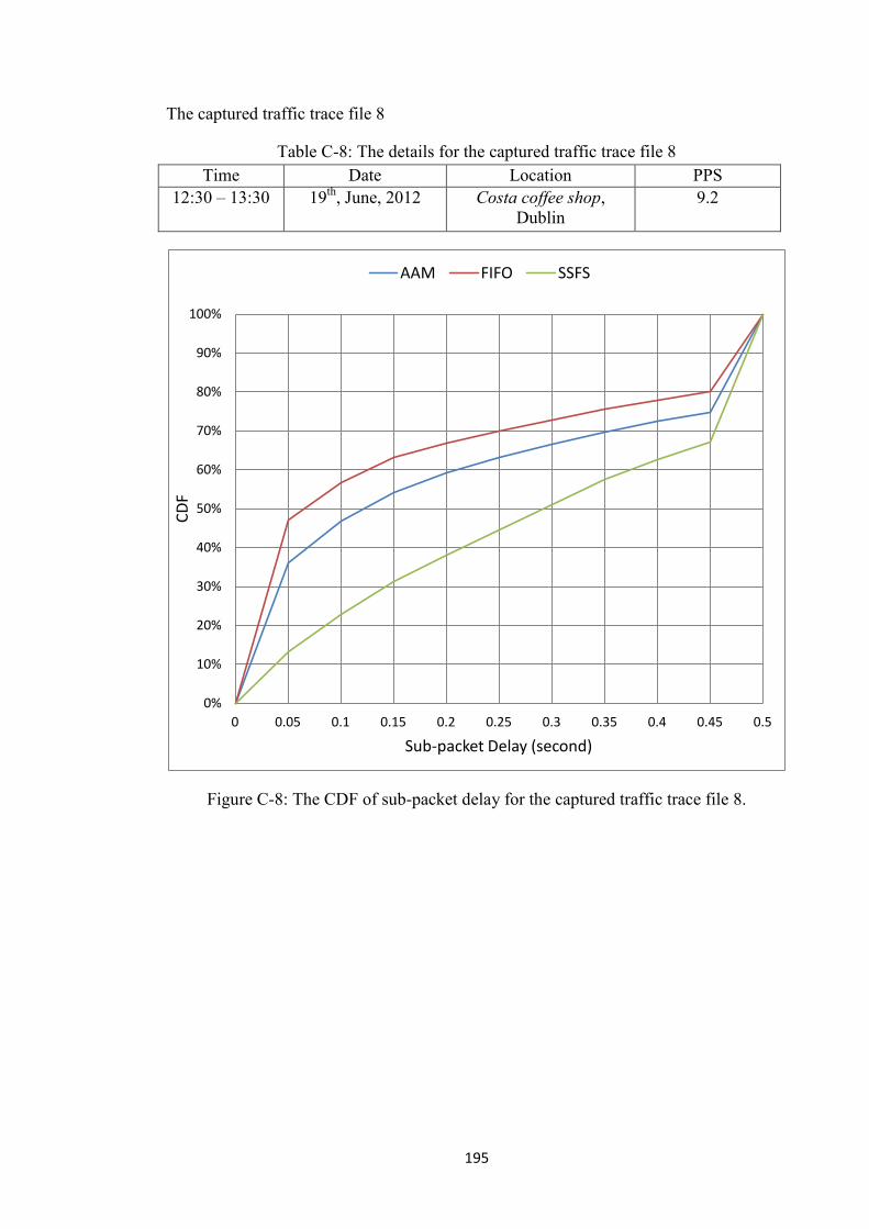
195
The captured traffic trace file 8
Table C-8: The details for the captured traffic trace file 8
Time Date Location PPS
12:30 – 13:30 19th
, June, 2012 Costa coffee shop,
Dublin
9.2
Figure C-8: The CDF of sub-packet delay for the captured traffic trace file 8.
0%
10%
20%
30%
40%
50%
60%
70%
80%
90%
100%
0 0.05 0.1 0.15 0.2 0.25 0.3 0.35 0.4 0.45 0.5
CD
F
Sub-packet Delay (second)
AAM FIFO SSFS

196
The captured traffic trace file 9
Table C-9: The details for the captured traffic trace file 9
Time Date Location PPS
16:00 –17:00 19th
, June, 2012 Parliament Square, TCD,
Dublin
3.6
Figure C-9: The CDF of sub-packet delay for the captured traffic trace file 9.
0%
10%
20%
30%
40%
50%
60%
70%
80%
90%
100%
0 0.05 0.1 0.15 0.2 0.25 0.3 0.35 0.4 0.45 0.5
CD
F
Sub-packet Delay (second)
AAM FIFO SSFS

197
The captured traffic trace file 10
Table C-10: The details for the captured traffic trace file 10
Time Date Location PPS
17:00 – 18:00 19th
, June, 2012 Costa coffee shop,
Dublin
6.6
Figure C-10: The CDF of sub-packet delay for the captured traffic trace file 10.
0%
10%
20%
30%
40%
50%
60%
70%
80%
90%
100%
0 0.05 0.1 0.15 0.2 0.25 0.3 0.35 0.4 0.45 0.5
CD
F
Sub-packet Delay (second)
AAM FIFO SSFS
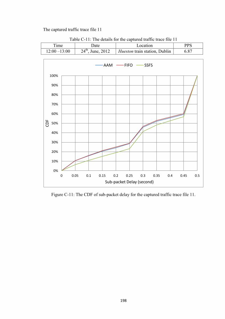
198
The captured traffic trace file 11
Table C-11: The details for the captured traffic trace file 11
Time Date Location PPS
12:00 –13:00 24th
, June, 2012 Hueston train station, Dublin 6.87
Figure C-11: The CDF of sub-packet delay for the captured traffic trace file 11.
0%
10%
20%
30%
40%
50%
60%
70%
80%
90%
100%
0 0.05 0.1 0.15 0.2 0.25 0.3 0.35 0.4 0.45 0.5
CD
F
Sub-packet Delay (second)
AAM FIFO SSFS
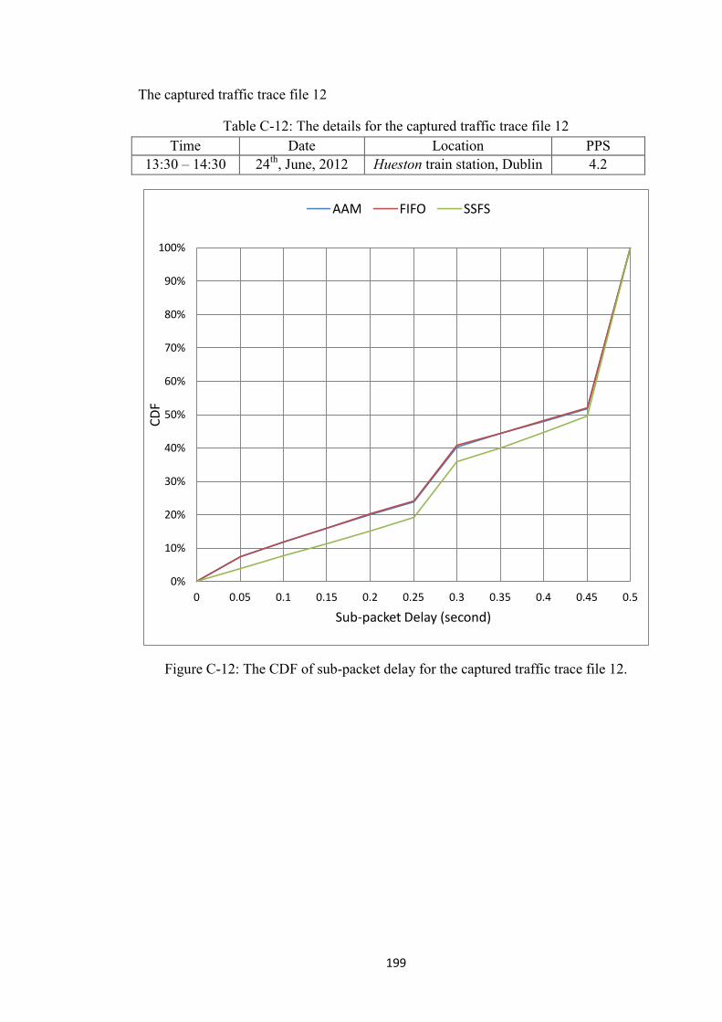
199
The captured traffic trace file 12
Table C-12: The details for the captured traffic trace file 12
Time Date Location PPS
13:30 – 14:30 24th
, June, 2012 Hueston train station, Dublin 4.2
Figure C-12: The CDF of sub-packet delay for the captured traffic trace file 12.
0%
10%
20%
30%
40%
50%
60%
70%
80%
90%
100%
0 0.05 0.1 0.15 0.2 0.25 0.3 0.35 0.4 0.45 0.5
CD
F
Sub-packet Delay (second)
AAM FIFO SSFS
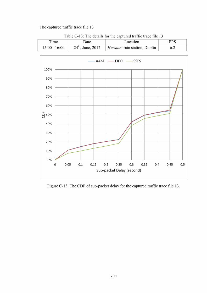
200
The captured traffic trace file 13
Table C-13: The details for the captured traffic trace file 13
Time Date Location PPS
15:00 –16:00 24th
, June, 2012 Hueston train station, Dublin 6.2
Figure C-13: The CDF of sub-packet delay for the captured traffic trace file 13.
0%
10%
20%
30%
40%
50%
60%
70%
80%
90%
100%
0 0.05 0.1 0.15 0.2 0.25 0.3 0.35 0.4 0.45 0.5
CD
F
Sub-packet Delay (second)
AAM FIFO SSFS

201
The captured traffic trace file 14
Table C-14: The details for the captured traffic trace file 14
Time Date Location PPS
10:30 –11:30 26th
, June, 2012 Library, Kevin street, DIT,
Dublin
19.2
Figure C-14: The CDF of sub-packet delay for the captured traffic trace file 14.
0%
10%
20%
30%
40%
50%
60%
70%
80%
90%
100%
0 0.05 0.1 0.15 0.2 0.25 0.3 0.35 0.4 0.45 0.5
CD
F
Sub-packet Delay (second)
AAM FIFO SSFS

202
The captured traffic trace file 15
Table C-15: The details for the captured traffic trace file 15
Time Date Location PPS
12:00 –13:00 26th
, June, 2012 Library, Kevin street, DIT,
Dublin
3.8
Figure C-15: The CDF of sub-packet delay for the captured traffic trace file 15.
0%
10%
20%
30%
40%
50%
60%
70%
80%
90%
100%
0 0.05 0.1 0.15 0.2 0.25 0.3 0.35 0.4 0.45 0.5
CD
F
Sub-packet Delay (second)
AAM FIFO SSFS

203
The captured traffic trace file 16
Table C-16: The details for the captured traffic trace file 16
Time Date Location PPS
19:00 –19:50 17th
,July, 2012 Shuangliu airport, Sichuan,
China
6.9
Figure C-16: The CDF of sub-packet delay for the captured traffic trace file 16.
0%
10%
20%
30%
40%
50%
60%
70%
80%
90%
100%
0 0.05 0.1 0.15 0.2 0.25 0.3 0.35 0.4 0.45 0.5
CD
F
Sub-packet Delay (second)
AAM FIFO SSFS

204
Appendix D
The captured traffic trace file 1
Table D-1: The details for the captured traffic trace file 1
Time Date Location PPS
10:30 – 11:30 29th
,May, 2012 JAVA City, DIT, Dublin 92.1
Figure D-1: The number of sub-packets against the average packet delay for the
captured traffic trace file1.
0
0.05
0.1
0.15
0.2
0.25
0.3
0.35
0.4
0.45
0.5
1 2 3 4 5 6 7 8 9 10 11 12 13
Ave
rage
Pac
ket
Del
ay (
seco
nd
)
Number of Sub-packets
AAM SSFS FIFO
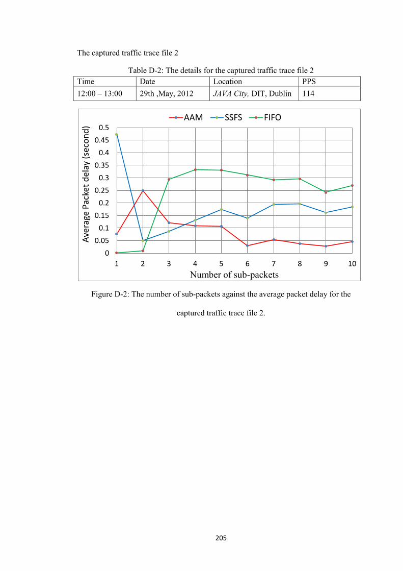
205
The captured traffic trace file 2
Table D-2: The details for the captured traffic trace file 2
Time Date Location PPS
12:00 – 13:00 29th ,May, 2012 JAVA City, DIT, Dublin 114
Figure D-2: The number of sub-packets against the average packet delay for the
captured traffic trace file 2.
0
0.05
0.1
0.15
0.2
0.25
0.3
0.35
0.4
0.45
0.5
1 2 3 4 5 6 7 8 9 10
Ave
rage
Pac
ket
del
ay (
seco
nd
)
Number of sub-packets
AAM SSFS FIFO
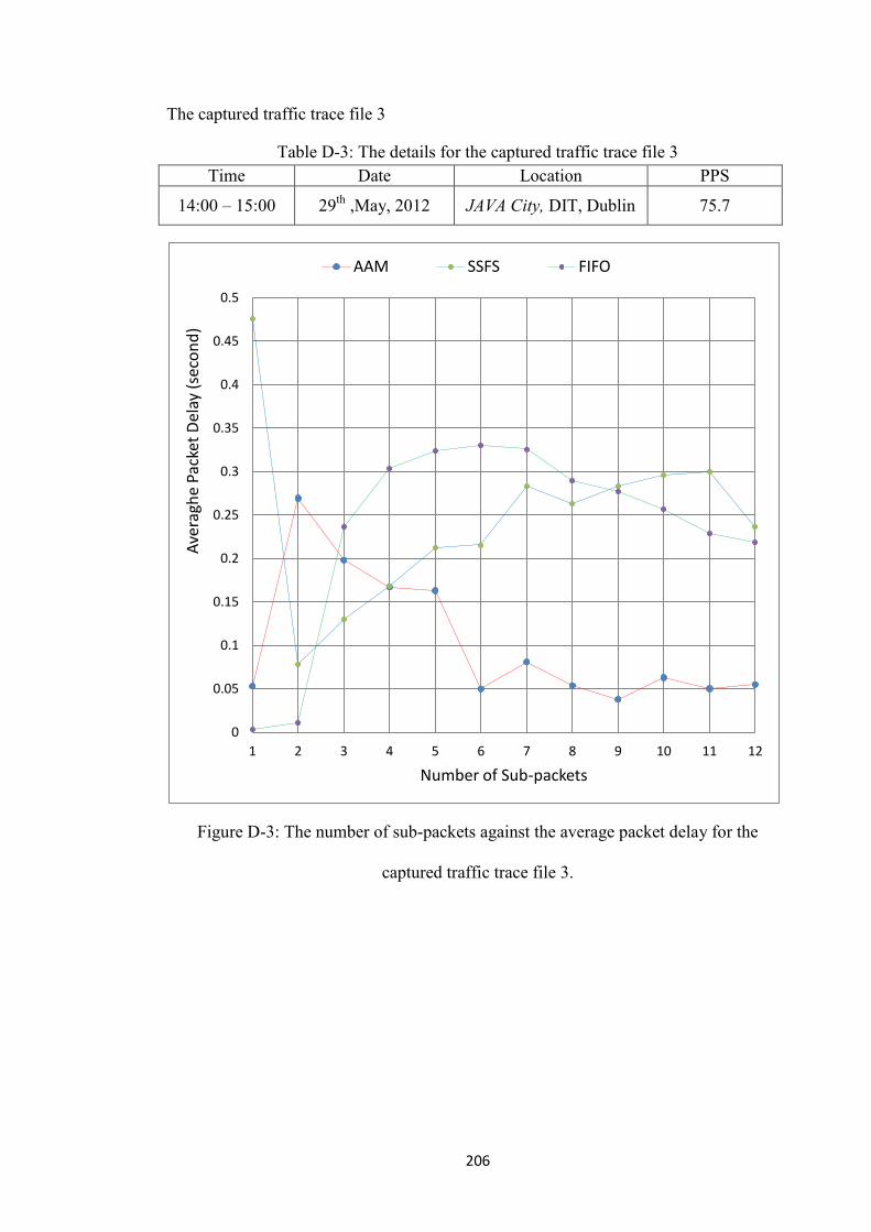
206
The captured traffic trace file 3
Table D-3: The details for the captured traffic trace file 3
Time Date Location PPS
14:00 – 15:00 29th
,May, 2012 JAVA City, DIT, Dublin 75.7
Figure D-3: The number of sub-packets against the average packet delay for the
captured traffic trace file 3.
0
0.05
0.1
0.15
0.2
0.25
0.3
0.35
0.4
0.45
0.5
1 2 3 4 5 6 7 8 9 10 11 12
Ave
ragh
e P
acke
t D
elay
(se
con
d)
Number of Sub-packets
AAM SSFS FIFO
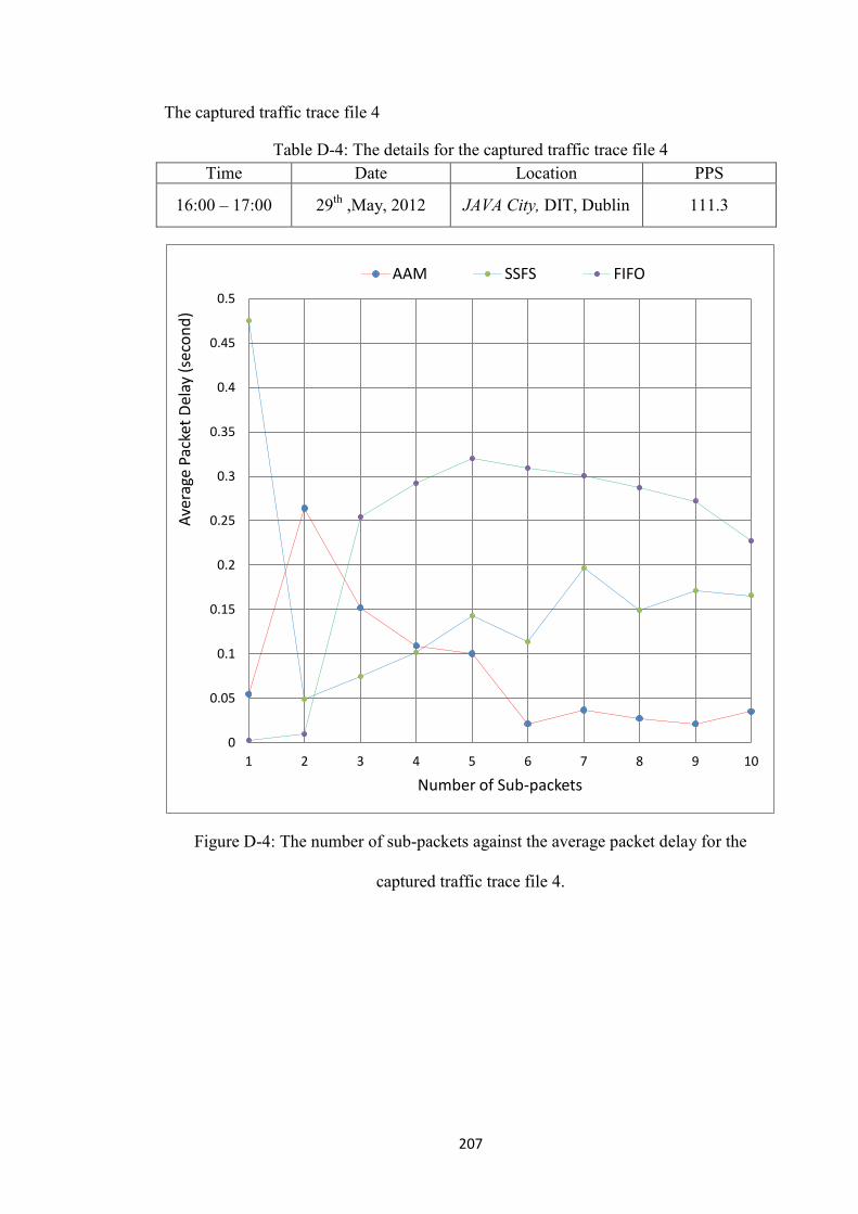
207
The captured traffic trace file 4
Table D-4: The details for the captured traffic trace file 4
Time Date Location PPS
16:00 – 17:00 29th
,May, 2012 JAVA City, DIT, Dublin 111.3
Figure D-4: The number of sub-packets against the average packet delay for the
captured traffic trace file 4.
0
0.05
0.1
0.15
0.2
0.25
0.3
0.35
0.4
0.45
0.5
1 2 3 4 5 6 7 8 9 10
Ave
rage
Pac
ket
Del
ay (
seco
nd
)
Number of Sub-packets
AAM SSFS FIFO
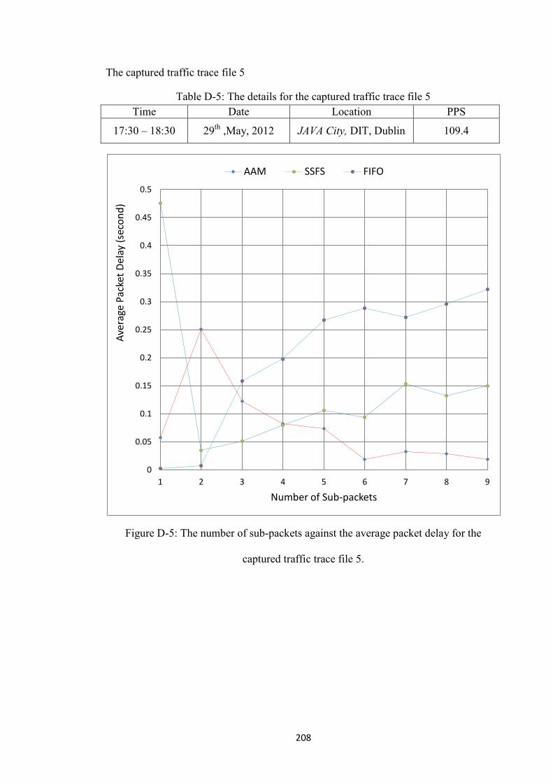
208
The captured traffic trace file 5
Table D-5: The details for the captured traffic trace file 5
Time Date Location PPS
17:30 – 18:30 29th
,May, 2012 JAVA City, DIT, Dublin 109.4
Figure D-5: The number of sub-packets against the average packet delay for the
captured traffic trace file 5.
0
0.05
0.1
0.15
0.2
0.25
0.3
0.35
0.4
0.45
0.5
1 2 3 4 5 6 7 8 9
Ave
rage
Pac
ket
Del
ay (
seco
nd
)
Number of Sub-packets
AAM SSFS FIFO

209
The captured traffic trace file 6
Table D-6: The details for the captured traffic trace file 6
Time Date Location PPS
09:30 – 10:30 19th
, June, 2012 Costa coffee shop,
Dublin 9.4
Figure D-6: The number of sub-packets against the average packet delay for the
captured traffic trace file 6.
0
0.05
0.1
0.15
0.2
0.25
0.3
0.35
0.4
0.45
0.5
1 2 3 4 5 6 7 8 9 10 11 12 13 14
Ave
rage
Pac
ket
Del
ay (
seco
nd
)
Number of Sub-packets
AAM SSFS FIFO
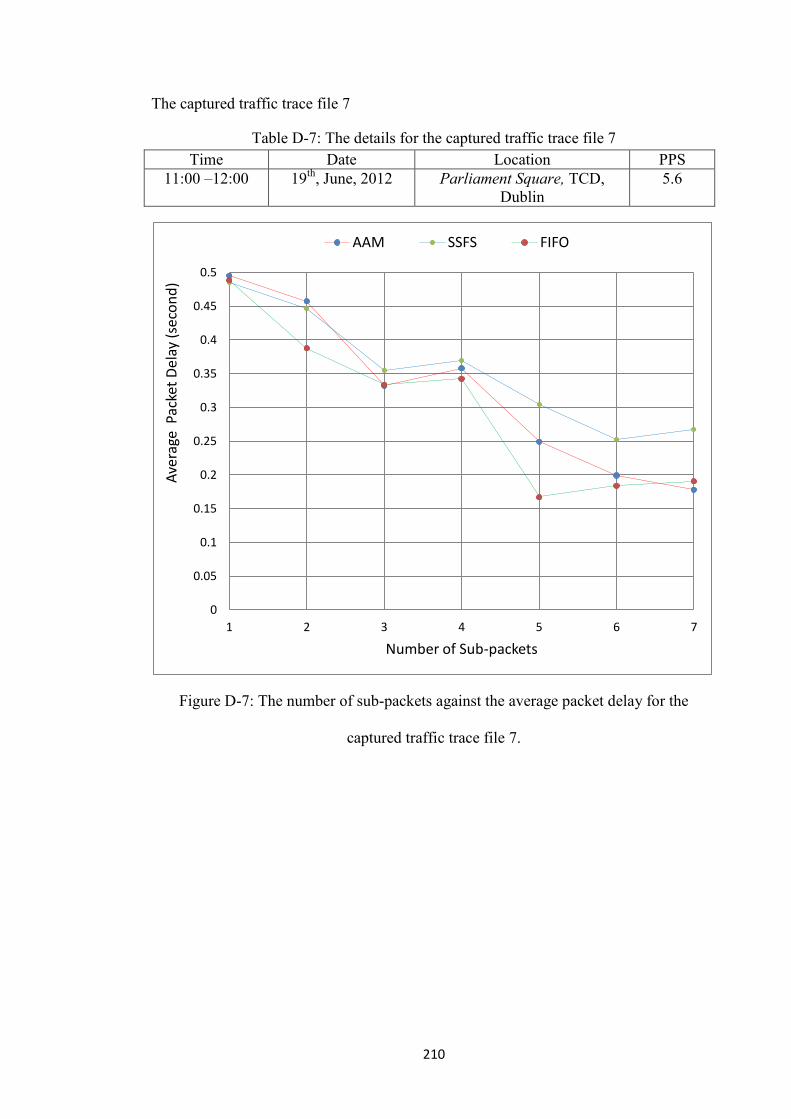
210
The captured traffic trace file 7
Table D-7: The details for the captured traffic trace file 7
Time Date Location PPS
11:00 –12:00 19th
, June, 2012 Parliament Square, TCD,
Dublin
5.6
Figure D-7: The number of sub-packets against the average packet delay for the
captured traffic trace file 7.
0
0.05
0.1
0.15
0.2
0.25
0.3
0.35
0.4
0.45
0.5
1 2 3 4 5 6 7
Ave
rage
Pac
ket
Del
ay (
seco
nd
)
Number of Sub-packets
AAM SSFS FIFO

211
The captured traffic trace file 8
Table D-8: The details for the captured traffic trace file 8
Time Date Location PPS
12:30 – 13:30 19th
, June, 2012 Costa coffee shop,
Dublin 9.2
Figure D-8: The number of sub-packets against the average packet delay for the
captured traffic trace file8.
0
0.05
0.1
0.15
0.2
0.25
0.3
0.35
0.4
0.45
0.5
1 2 3 4 5 6 7 8 9 10 11 12
Ave
rage
Pac
ket
Del
ay (
seco
nd
)
Number of Sub-packets
AAM SSFS FIFO
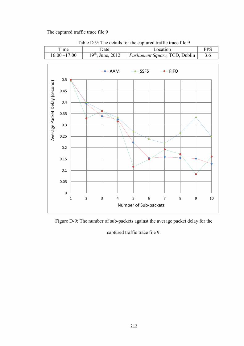
212
The captured traffic trace file 9
Table D-9: The details for the captured traffic trace file 9
Time Date Location PPS
16:00 –17:00 19th
, June, 2012 Parliament Square, TCD, Dublin 3.6
Figure D-9: The number of sub-packets against the average packet delay for the
captured traffic trace file 9.
0
0.05
0.1
0.15
0.2
0.25
0.3
0.35
0.4
0.45
0.5
1 2 3 4 5 6 7 8 9 10
Ave
rage
Pac
ket
Del
ay (
seco
nd
)
Number of Sub-packets
AAM SSFS FIFO
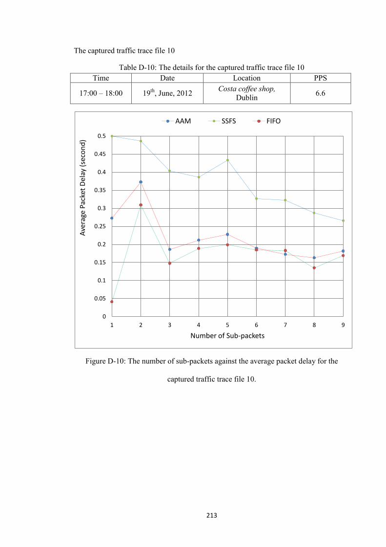
213
The captured traffic trace file 10
Table D-10: The details for the captured traffic trace file 10
Time Date Location PPS
17:00 – 18:00 19th
, June, 2012 Costa coffee shop,
Dublin 6.6
Figure D-10: The number of sub-packets against the average packet delay for the
captured traffic trace file 10.
0
0.05
0.1
0.15
0.2
0.25
0.3
0.35
0.4
0.45
0.5
1 2 3 4 5 6 7 8 9
Ave
rage
Pac
ket
Del
ay (
seco
nd
)
Number of Sub-packets
AAM SSFS FIFO

214
The captured traffic trace file 11
Table D-11: The details for the captured traffic trace file 11
Time Date Location PPS
12:00 –13:00 24th
, June, 2012 Hueston train station,
Dublin 6.87
Figure D-11: The number of sub-packets against the average packet delay for the
captured traffic trace file 11.
0
0.05
0.1
0.15
0.2
0.25
0.3
0.35
0.4
0.45
0.5
1 2 3 4 5 6 7 8 9 10 11 12 13 14
Ave
rage
Pac
ket
Del
ay (
seco
nd
)
Number of Sub-packets
AAM SSFS FIFO
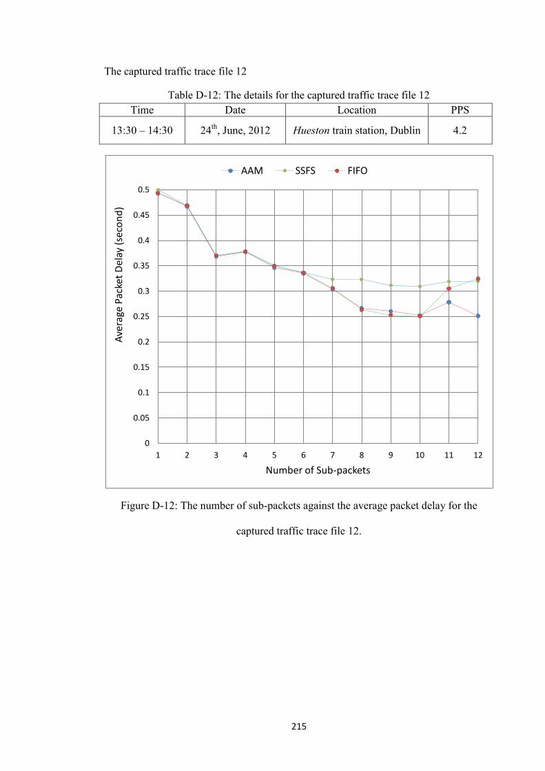
215
The captured traffic trace file 12
Table D-12: The details for the captured traffic trace file 12
Time Date Location PPS
13:30 – 14:30 24th
, June, 2012 Hueston train station, Dublin 4.2
Figure D-12: The number of sub-packets against the average packet delay for the
captured traffic trace file 12.
0
0.05
0.1
0.15
0.2
0.25
0.3
0.35
0.4
0.45
0.5
1 2 3 4 5 6 7 8 9 10 11 12
Ave
rage
Pac
ket
Del
ay (
seco
nd
)
Number of Sub-packets
AAM SSFS FIFO

216
The captured traffic trace file 13
Table D-13: The details for the captured traffic trace file 13
Time Date Location PPS
15:00 –16:00 24th
, June, 2012 Hueston train station,
Dublin 6.2
Figure D-13: The number of sub-packets against the average packet delay for the
captured traffic trace file 13.
0
0.05
0.1
0.15
0.2
0.25
0.3
0.35
0.4
0.45
0.5
1 2 3 4 5 6 7 8 9 10
Ave
rage
Pac
ket
Del
ay (
seco
nd
)
Number of Sub-packets
AAM SSFS FIFO
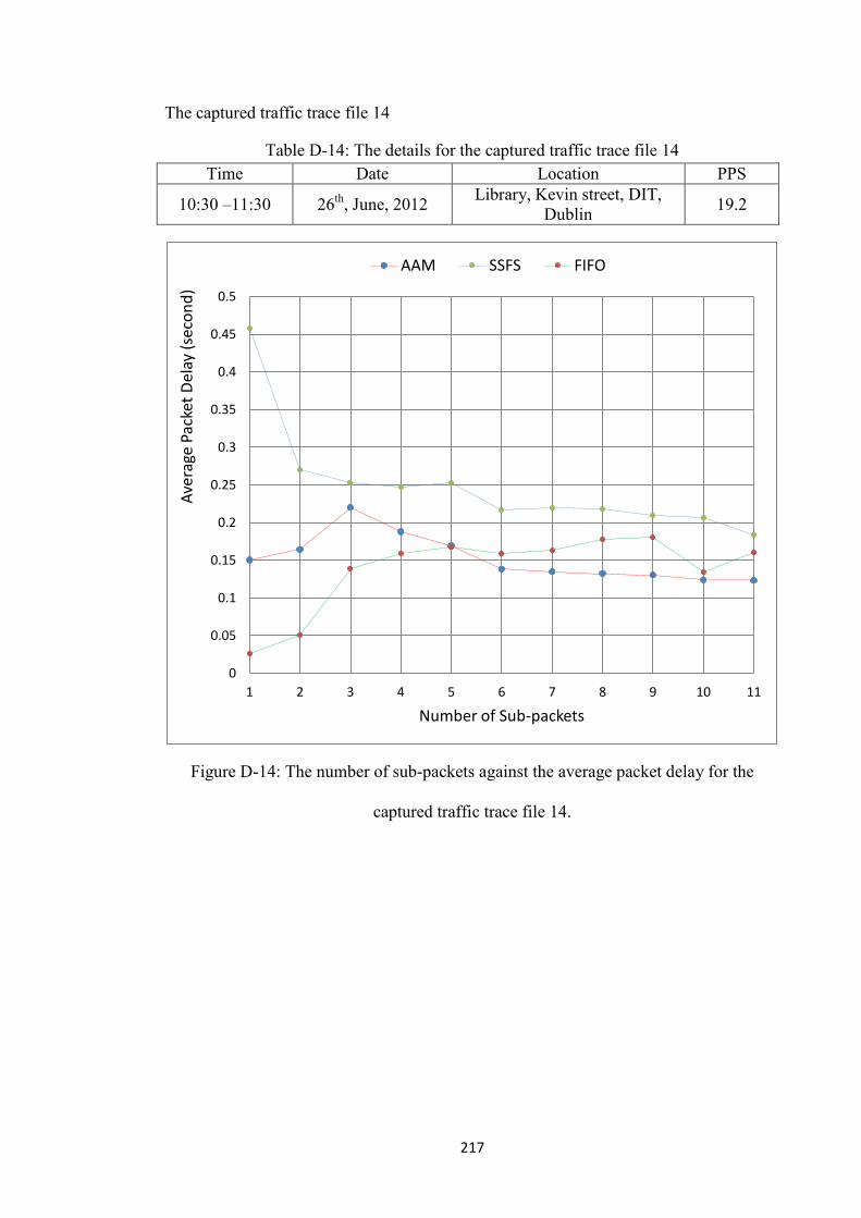
217
The captured traffic trace file 14
Table D-14: The details for the captured traffic trace file 14
Time Date Location PPS
10:30 –11:30 26th
, June, 2012 Library, Kevin street, DIT,
Dublin 19.2
Figure D-14: The number of sub-packets against the average packet delay for the
captured traffic trace file 14.
0
0.05
0.1
0.15
0.2
0.25
0.3
0.35
0.4
0.45
0.5
1 2 3 4 5 6 7 8 9 10 11
Ave
rage
Pac
ket
Del
ay (
seco
nd
)
Number of Sub-packets
AAM SSFS FIFO
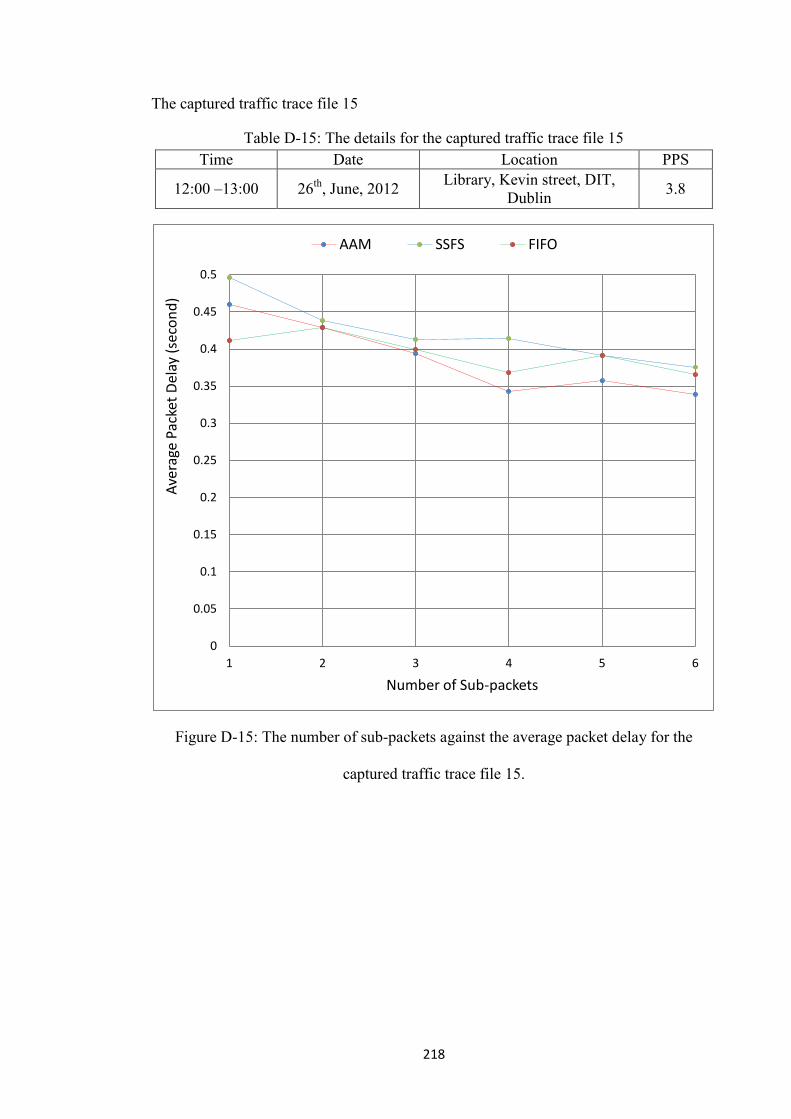
218
The captured traffic trace file 15
Table D-15: The details for the captured traffic trace file 15
Time Date Location PPS
12:00 –13:00 26th
, June, 2012 Library, Kevin street, DIT,
Dublin 3.8
Figure D-15: The number of sub-packets against the average packet delay for the
captured traffic trace file 15.
0
0.05
0.1
0.15
0.2
0.25
0.3
0.35
0.4
0.45
0.5
1 2 3 4 5 6
Ave
rage
Pac
ket
Del
ay (
seco
nd
)
Number of Sub-packets
AAM SSFS FIFO
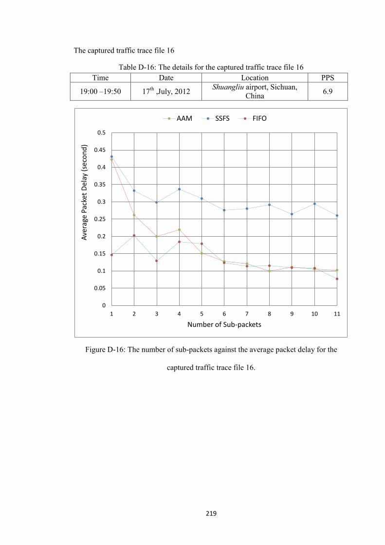
219
The captured traffic trace file 16
Table D-16: The details for the captured traffic trace file 16
Time Date Location PPS
19:00 –19:50 17th
,July, 2012 Shuangliu airport, Sichuan,
China 6.9
Figure D-16: The number of sub-packets against the average packet delay for the
captured traffic trace file 16.
0
0.05
0.1
0.15
0.2
0.25
0.3
0.35
0.4
0.45
0.5
1 2 3 4 5 6 7 8 9 10 11
Ave
rage
Pac
ket
Del
ay (
seco
nd
)
Number of Sub-packets
AAM SSFS FIFO