An accurate and efficient Lagrangian sub-grid model

Citation for published version (APA):Mazzitelli, I. M., Toschi, F., & Lanotte, A. S. (2014). An accurate and efficient Lagrangian sub-grid model.Physics of Fluids, 26(9), 095101-1/17. DOI: 10.1063/1.4894149

DOI:10.1063/1.4894149

Document status and date:Published: 01/01/2014

Document Version:Publisher’s PDF, also known as Version of Record (includes final page, issue and volume numbers)

Please check the document version of this publication:

• A submitted manuscript is the version of the article upon submission and before peer-review. There can beimportant differences between the submitted version and the official published version of record. Peopleinterested in the research are advised to contact the author for the final version of the publication, or visit theDOI to the publisher's website.• The final author version and the galley proof are versions of the publication after peer review.• The final published version features the final layout of the paper including the volume, issue and pagenumbers.Link to publication

General rightsCopyright and moral rights for the publications made accessible in the public portal are retained by the authors and/or other copyright ownersand it is a condition of accessing publications that users recognise and abide by the legal requirements associated with these rights.

• Users may download and print one copy of any publication from the public portal for the purpose of private study or research. • You may not further distribute the material or use it for any profit-making activity or commercial gain • You may freely distribute the URL identifying the publication in the public portal.

If the publication is distributed under the terms of Article 25fa of the Dutch Copyright Act, indicated by the “Taverne” license above, pleasefollow below link for the End User Agreement:

www.tue.nl/taverne

Take down policyIf you believe that this document breaches copyright please contact us at:

openaccess@tue.nl

providing details and we will investigate your claim.

Download date: 18. Feb. 2019

PHYSICS OF FLUIDS 26, 095101 (2014)

An accurate and efficient Lagrangian sub-grid modelIrene M. Mazzitelli,1 Federico Toschi,2 and Alessandra S. Lanotte3,a)

1Dip. Ingegneria dell’Innovazione, Univ. Salento, 73100 Lecce, Italy and CNR-ISAC,Via Fosso del Cavaliere 100, 00133 Roma, Italy2Department of Applied Physics and Department of Mathematics and Computer Science,Eindhoven University of Technology, Eindhoven 5600 MB, The Netherlands and CNR-IAC,Via dei Taurini 19, 00185 Rome, Italy3CNR ISAC and INFN, Sez. di Lecce, Str. Prov. Lecce Monteroni, 73100 Lecce, Italy

(Received 18 February 2014; accepted 18 August 2014; published online 3 September 2014)

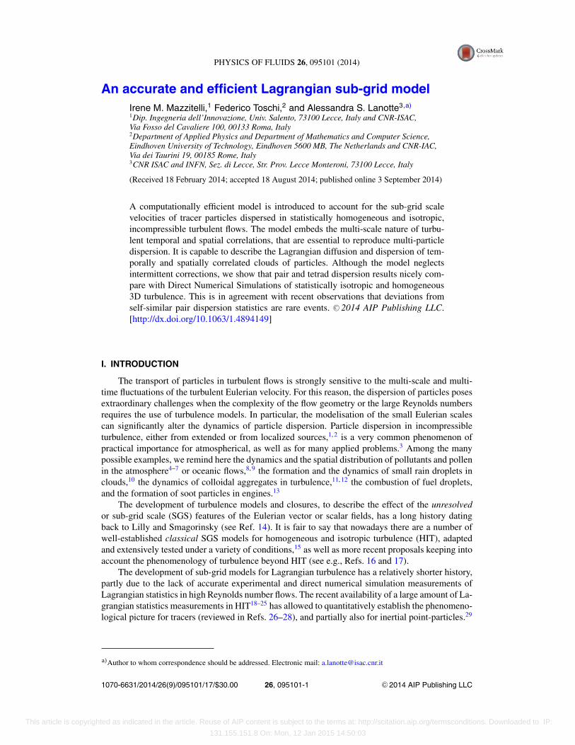
A computationally efficient model is introduced to account for the sub-grid scalevelocities of tracer particles dispersed in statistically homogeneous and isotropic,incompressible turbulent flows. The model embeds the multi-scale nature of turbu-lent temporal and spatial correlations, that are essential to reproduce multi-particledispersion. It is capable to describe the Lagrangian diffusion and dispersion of tem-porally and spatially correlated clouds of particles. Although the model neglectsintermittent corrections, we show that pair and tetrad dispersion results nicely com-pare with Direct Numerical Simulations of statistically isotropic and homogeneous3D turbulence. This is in agreement with recent observations that deviations fromself-similar pair dispersion statistics are rare events. C© 2014 AIP Publishing LLC.[http://dx.doi.org/10.1063/1.4894149]

I. INTRODUCTION

The transport of particles in turbulent flows is strongly sensitive to the multi-scale and multi-time fluctuations of the turbulent Eulerian velocity. For this reason, the dispersion of particles posesextraordinary challenges when the complexity of the flow geometry or the large Reynolds numbersrequires the use of turbulence models. In particular, the modelisation of the small Eulerian scalescan significantly alter the dynamics of particle dispersion. Particle dispersion in incompressibleturbulence, either from extended or from localized sources,1, 2 is a very common phenomenon ofpractical importance for atmospherical, as well as for many applied problems.3 Among the manypossible examples, we remind here the dynamics and the spatial distribution of pollutants and pollenin the atmosphere4–7 or oceanic flows,8, 9 the formation and the dynamics of small rain droplets inclouds,10 the dynamics of colloidal aggregates in turbulence,11, 12 the combustion of fuel droplets,and the formation of soot particles in engines.13

The development of turbulence models and closures, to describe the effect of the unresolvedor sub-grid scale (SGS) features of the Eulerian vector or scalar fields, has a long history datingback to Lilly and Smagorinsky (see Ref. 14). It is fair to say that nowadays there are a number ofwell-established classical SGS models for homogeneous and isotropic turbulence (HIT), adaptedand extensively tested under a variety of conditions,15 as well as more recent proposals keeping intoaccount the phenomenology of turbulence beyond HIT (see e.g., Refs. 16 and 17).

The development of sub-grid models for Lagrangian turbulence has a relatively shorter history,partly due to the lack of accurate experimental and direct numerical simulation measurements ofLagrangian statistics in high Reynolds number flows. The recent availability of a large amount of La-grangian statistics measurements in HIT18–25 has allowed to quantitatively establish the phenomeno-logical picture for tracers (reviewed in Refs. 26–28), and partially also for inertial point-particles.29

a)Author to whom correspondence should be addressed. Electronic mail: a.lanotte@isac.cnr.it

1070-6631/2014/26(9)/095101/17/$30.00 C©2014 AIP Publishing LLC26, 095101-1

This article is copyrighted as indicated in the article. Reuse of AIP content is subject to the terms at: http://scitation.aip.org/termsconditions. Downloaded to IP:

131.155.151.8 On: Mon, 12 Jan 2015 14:50:03

095101-2 Mazzitelli, Toschi, and Lanotte Phys. Fluids 26, 095101 (2014)

The knowledge borrowed from experiments and direct numerical simulations has then promotednew research on Lagrangian sub-grid scale models for tracers, and inertial particles also (see e.g.,Refs. 6, 30, and 31). The effects of small-scale temporal and spatial correlations on the dynamics ofparticles are an important problem.32 In particular beyond classical measurements of the Lagrangiandynamics of a single particle and of particle pairs, the geometric features of multiparticles dispersionhas also been investigated.33–36

Within the complex picture of Lagrangian dynamics, one of the most important point is thatLagrangian turbulence is more intermittent than Eulerian turbulence37 and, as a result, one mayhave to pay additional care when using Gaussian models to model the Lagrangian velocity fields.Moreover, in HIT, the relative dispersion of tracers is mainly dominated by small-scale fluid motions:if these are neglected, particle pairs disperse at a much slower rate than the actual one (ballistic vsRichardson dispersion).

Traditionally, Lagrangian SGS motions are described by means of stochastic models. These arebased on stochastic differential equations for the evolution of the velocity, assumed to be Markovian,along a particle trajectory. Stochastic models can be built up for single particle trajectories,38 two-particle39–41 and four-particle dispersion.42, 43 The literature on the topic is vast and we cannotreview it here. What is important for the present discussion is that stochastic models for two-particledispersion are generally inconsistent with single particle statistics, so that depending on the problemat hand one has to change model.

A different approach was developed in Lacorata et al.,6 where a multiscale kinematic velocityfield was introduced to model turbulent relative dispersion at sub-grid scales. The authors exploitedLagrangian chaotic mixing generated by a nonlinear deterministic function, periodic in space andtime. This approach differs from kinematic models (e.g., Refs. 44 and 45), as it reproduces the effectof large-scale sweeping on particle trajectories.46–48

In the context of wall-bounded flows, Lagrangian SGS schemes have been proposed in termsof approximate deconvolution models based on the Eulerian field (see, e.g., Ref. 49), or in terms offorce-based models.50 Observables capable to discriminate between model error and drift inducederrors were proposed.51

Most of these models rely on the knowledge of the resolved Eulerian velocity field. However,we note that models have been proposed to solve the Lagrangian dynamics self-consistently withoutan underlying Eulerian velocity field. This is for example the idea behind Smoothed Particle Hy-drodynamics (SPH), i.e., a purely Lagrangian scheme to solve the Navier-Stokes equation, recentlyreviewed in Ref. 52. In Smoothed Particle Hydrodynamics, instead of solving the fluid equations ona grid, a set of particles are used , whose equations of motion are determined from the continuumNavier-Stokes equations.

An important issue concerns the possibility to build up models accounting for multi-particledispersion, N > 2, going beyond the pair separation dynamics. Multi-particle Lagrangian modelsinvariably need to incorporate a mechanism correlating the sub-grid-scale velocities of the particles.Different approaches are possible. In Sawford et al.,53 a two-particle stochastic model for 3DGaussian turbulence40, 54 has been generalised to the problem of N tracers: these are constrained bypair-wise spatial correlations, implying that multi-point correlations are neglected. Interestingly, themodel shows a good agreement of multi-point statistics with direct numerical simulations results.Alternatively, Burgener et al.55 proposed to build spatial correlations between the fluid particles byminimising a Heisenberg-like Hamiltonian. In the Hamiltonian, the two-object coupling function isdistance-dependent and with a power law behaviour. Ballistic separation and Taylor diffusion regimesin pair dispersion are clearly observed, while turbulent inertial-range dispersion a la Richardson isobserved in specific conditions, only.

In this paper, we introduce a novel, accurate, and computationally efficient Lagrangian Sub-GridScale model (LSGS) for the dispersion of an arbitrary number of tracers in 3D statistically homo-geneous and isotropic turbulent flows. The model is purely Lagrangian and it defines and evolvesthe velocities of tracers at their positions. The trajectories of N particles are simply obtained bytime-integrating the Lagrangian velocities. It is primarily meant to reproduce Lagrangian dispersionat sub-grid scales, but it may be used as well as a rudimentary Lagrangian Navier-Stokes solver,much in the spirit of SPH.

This article is copyrighted as indicated in the article. Reuse of AIP content is subject to the terms at: http://scitation.aip.org/termsconditions. Downloaded to IP:

131.155.151.8 On: Mon, 12 Jan 2015 14:50:03

095101-3 Mazzitelli, Toschi, and Lanotte Phys. Fluids 26, 095101 (2014)

The model encodes velocity fluctuations that scale in space and in time consistently withKolmogorov’s 1941 theory,56 hence without intermittentcy corrections, and is self-consistent for anarbitrary number or density of tracers. An essential prescription for the model is the capability tocorrectly reproduce single-particle absolute diffusion together with multi-particle dispersion. For thelatter, we require proper reproduction of inertial range pair dispersion (Richardson dispersion25, 27, 28),as well as the dynamics and the deformation of tetrads.

In a nutshell, the idea of the LSGS model is to define a multiscale relative velocity differencebetween two tracers, consistent with Kolmogorov inertial range scaling. Such velocity difference,characterized by the proper eddy turnover time, is able to reproduce Richardson dispersion for asingle pair of tracers. The model is built up in a similar spirit of what done in Ref. 6 for tracerpair dispersion, but it is capable of ensuring consistent correlations between an arbitrary numberof tracers according to their positions and relative distances. By accounting for spatial correlationsamong nearby tracers, we ensure that tracers close in space will experience very similar SGSvelocities.

Beyond pair dispersion, we quantitatively validate the temporal evolution and dispersion proper-ties of groups of four particles (tetrads), against Direct Numerical Simulations results.34 An importantproperty of any Lagrangian model for incompressible turbulence is the maintenance of a uniformspatial distribution of tracer particles. This issue is related to the incompressibility of the modeledvelocity field. We investigate this issue at length in the Appendix. Our conclusion is that the degreeof homogeneity can be kept controlled, and that possible small deviations from uniformity becomenegligible when the model is used as a SGS model in large-eddy simulations or any other large-scalenumerical model.

The paper is organised as follows. In Sec. II, we introduce the LSGS model for an arbitrarynumber of tracers, and with an arbitrary large inertial range of scales. In Sec. III, we specify themodel parameters and discuss the results for absolute, pair, and tetrad dispersion. Section IV isdevoted to the concluding remarks.

II. THE LAGRANGIAN PARTICLE MODEL

In large-eddy simulations, the full tracer velocity is defined as the sum of the resolved Lagrangianvelocity component, V i (xi , t), and the sub-grid-scale contribution, vi (xi (t), t). The larger scalecomponents of the velocity, characterized by larger correlation times, sweep the smaller ones thusadvecting both particles and small-scale eddies. This is a crucial feature of Lagrangian turbulence,sometimes neglected in synthetic models of Eulerian turbulence, that incorrectly describe pairdispersion.46–48

The Lagrangian sub-grid-scale model describes the 3D velocity, vi (xi (t), t), at the position,xi (t), of the ith of the N tracer particles. The velocity fluctuations along each particle trajectory arethe superposition of different contributions from eddies of different sizes. These eddies constitute aturbulent field, decomposed for convenience in terms of logarithmically spaced shells.

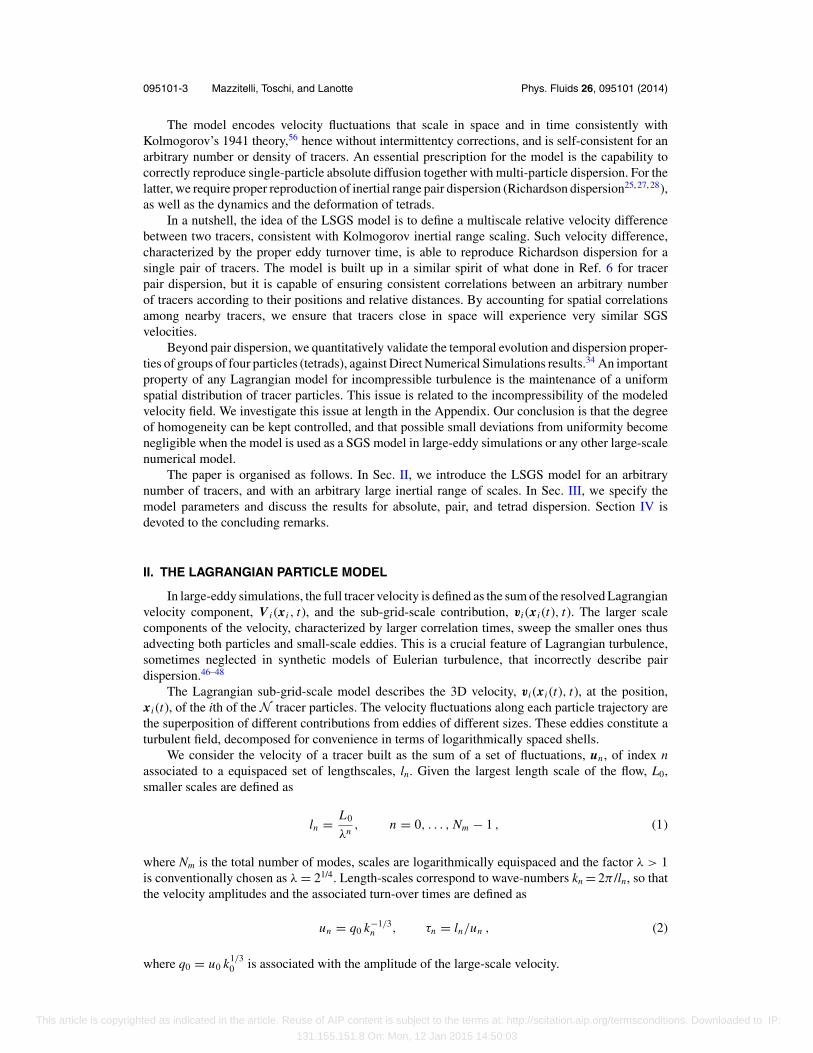
We consider the velocity of a tracer built as the sum of a set of fluctuations, un , of index nassociated to a equispaced set of lengthscales, ln. Given the largest length scale of the flow, L0,smaller scales are defined as

ln = L0

λn, n = 0, . . . , Nm − 1 , (1)

where Nm is the total number of modes, scales are logarithmically equispaced and the factor λ > 1is conventionally chosen as λ = 21/4. Length-scales correspond to wave-numbers kn = 2π /ln, so thatthe velocity amplitudes and the associated turn-over times are defined as

un = q0 k−1/3n , τn = ln/un , (2)

where q0 = u0 k1/30 is associated with the amplitude of the large-scale velocity.

This article is copyrighted as indicated in the article. Reuse of AIP content is subject to the terms at: http://scitation.aip.org/termsconditions. Downloaded to IP:

131.155.151.8 On: Mon, 12 Jan 2015 14:50:03

095101-4 Mazzitelli, Toschi, and Lanotte Phys. Fluids 26, 095101 (2014)

A. Implementation of the LSGS

With the aim of making the description as clear as possible, we consider that the model is bestillustrated by the following two-steps procedure:

Step 1: At time t, the positions xi(t) of all N particles are given. The algorithm then generates—for each tracer i and for each lengthscale ln—a first set of velocity vectors ζ (i)

n (t) (the three velocitycomponents along the space directions x, y, z that are chosen independently from each other). Eachof these velocities is the outcome of an Ornstein-Uhlenbeck (OU) process with correlation timeτ n = ln/un and variance u2

n , at the scale ln. The time evolution of the OU process, for each spatialcomponent of the velocity field of the ith particle at lengthscale ln, is obtained according to57

ζ (i)n (t + dt) = ζ (i)

n (t) e−dt/τn + un

√1 − e−2dt/τn β , (3)

where, for simplicity, we have omitted the sub-script for the spatial components. In (3), the variableβ is a random number, normally distributed in the range [0; 1]. According to our definitions, eachOU process is a normally distributed, random variable, ζ (i)

n (t), whose mean value μ(i)n and standard

deviation σ (i)n are :

μ(i)n = ζn0 exp [−(t − t0)/τn] , (4)

σ (i)n = un

√1 − exp [−2(t − t0)/τn]. (5)

The equilibrium time O(τ 0) is needed for each mode to relax to a zero mean velocity and to thevariance u2

n . The velocity associated to the ith tracer particle is the superposition of Nm modes givenby

v(i)(t) =Nm−1∑n=0

ζ (i)n (t) . (6)

So doing, each particle has a multiscale, single-point velocity field which has the physical timecorrelations, but which does not respect space correlations yet. Indeed, based on the above algorithm,very different velocity fields could be assigned to particles residing in very close spatial position.

Step 2: In order to build up the proper spatial correlations and establish a correspondencebetween the modelled particle velocities and the two-point Eulerian statistics, we redefine for the ithparticle the fluctuation associated to the nth mode as follows:

v(i)n (t) =

N∑j=1

ζ ( j)n (t) · (

1 − fln (|xi − x j |))

. (7)

Here the decorrelation function is such that f(r) ∝ r for r � 1 and f(r) � 1 for r � 1. Its preciseshape is not important and it may be as well a linear function, e.g.:

f (r ) = |xi − x j |/ ln if |xi − x j | < ln, (8)

f (r ) = 1 if |xi − x j | ≥ ln. (9)

Note that in (7), the nth mode velocity fluctuation for the ith particle is determined by the valueof the nth mode velocity fluctuation of the particle j, with j = 1, . . . ,N spanning over the entireparticle ensemble. Clearly, only particles closeby matter, while particles located very far from theith particle will not matter.

The particle velocity resulting from the contributions of different eddies is then evaluated as

v(i)(t) =Nm−1∑n=0

1

A(i)n

v(i)n (t). (10)

This article is copyrighted as indicated in the article. Reuse of AIP content is subject to the terms at: http://scitation.aip.org/termsconditions. Downloaded to IP:

131.155.151.8 On: Mon, 12 Jan 2015 14:50:03

095101-5 Mazzitelli, Toschi, and Lanotte Phys. Fluids 26, 095101 (2014)

3

rab

rbc

rac 2

(b)

(a)

(c)

1

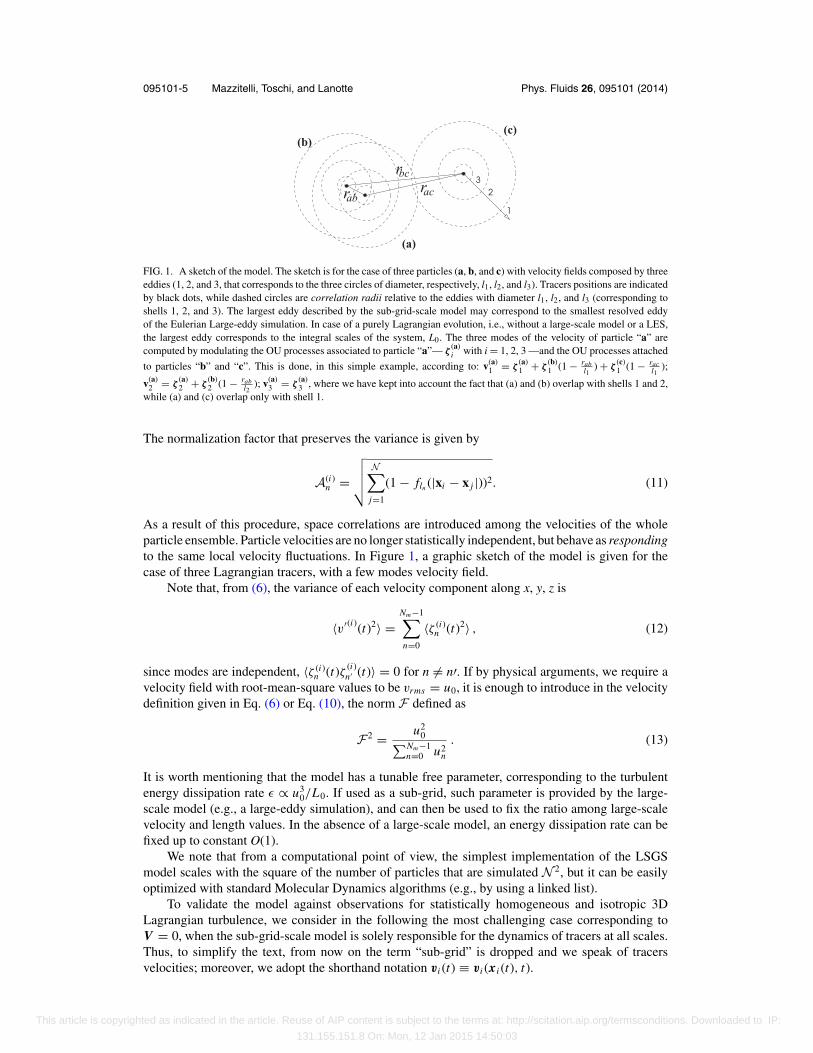
FIG. 1. A sketch of the model. The sketch is for the case of three particles (a, b, and c) with velocity fields composed by threeeddies (1, 2, and 3, that corresponds to the three circles of diameter, respectively, l1, l2, and l3). Tracers positions are indicatedby black dots, while dashed circles are correlation radii relative to the eddies with diameter l1, l2, and l3 (corresponding toshells 1, 2, and 3). The largest eddy described by the sub-grid-scale model may correspond to the smallest resolved eddyof the Eulerian Large-eddy simulation. In case of a purely Lagrangian evolution, i.e., without a large-scale model or a LES,the largest eddy corresponds to the integral scales of the system, L0. The three modes of the velocity of particle “a” arecomputed by modulating the OU processes associated to particle “a”— ζ

(a)i with i = 1, 2, 3 —and the OU processes attached

to particles “b” and “c”. This is done, in this simple example, according to: v(a)1 = ζ

(a)1 + ζ

(b)1 (1 − rab

l1) + ζ

(c)1 (1 − rac

l1);

v(a)2 = ζ

(a)2 + ζ

(b)2 (1 − rab

l2); v(a)

3 = ζ(a)3 , where we have kept into account the fact that (a) and (b) overlap with shells 1 and 2,

while (a) and (c) overlap only with shell 1.

The normalization factor that preserves the variance is given by

A(i)n =

√√√√ N∑j=1

(1 − fln (|xi − x j |))2. (11)

As a result of this procedure, space correlations are introduced among the velocities of the wholeparticle ensemble. Particle velocities are no longer statistically independent, but behave as respondingto the same local velocity fluctuations. In Figure 1, a graphic sketch of the model is given for thecase of three Lagrangian tracers, with a few modes velocity field.

Note that, from (6), the variance of each velocity component along x, y, z is

〈v′(i)(t)2〉 =Nm−1∑n=0

〈ζ (i)n (t)2〉 , (12)

since modes are independent, 〈ζ (i)n (t)ζ (i)

n′ (t)〉 = 0 for n = n′. If by physical arguments, we require avelocity field with root-mean-square values to be vrms = u0, it is enough to introduce in the velocitydefinition given in Eq. (6) or Eq. (10), the norm F defined as

F2 = u20∑Nm−1

n=0 u2n

. (13)

It is worth mentioning that the model has a tunable free parameter, corresponding to the turbulentenergy dissipation rate ε ∝ u3

0/L0. If used as a sub-grid, such parameter is provided by the large-scale model (e.g., a large-eddy simulation), and can then be used to fix the ratio among large-scalevelocity and length values. In the absence of a large-scale model, an energy dissipation rate can befixed up to constant O(1).

We note that from a computational point of view, the simplest implementation of the LSGSmodel scales with the square of the number of particles that are simulated N 2, but it can be easilyoptimized with standard Molecular Dynamics algorithms (e.g., by using a linked list).

To validate the model against observations for statistically homogeneous and isotropic 3DLagrangian turbulence, we consider in the following the most challenging case corresponding toV = 0, when the sub-grid-scale model is solely responsible for the dynamics of tracers at all scales.Thus, to simplify the text, from now on the term “sub-grid” is dropped and we speak of tracersvelocities; moreover, we adopt the shorthand notation vi (t) ≡ vi (xi (t), t).

This article is copyrighted as indicated in the article. Reuse of AIP content is subject to the terms at: http://scitation.aip.org/termsconditions. Downloaded to IP:

131.155.151.8 On: Mon, 12 Jan 2015 14:50:03

095101-6 Mazzitelli, Toschi, and Lanotte Phys. Fluids 26, 095101 (2014)

-0.20

0.20.40.6

v 1x-0.2

0

0.2

0.4

v 10x

0 0.05 0.1 0.15 0.2t / τ0

10-3

10-2

10-1

100

r(t)

/ L0

particle 1

particle 2

particle 1

particle 2

l1 / L0

l10 / L0

t10 / τ0 t1 / τ0

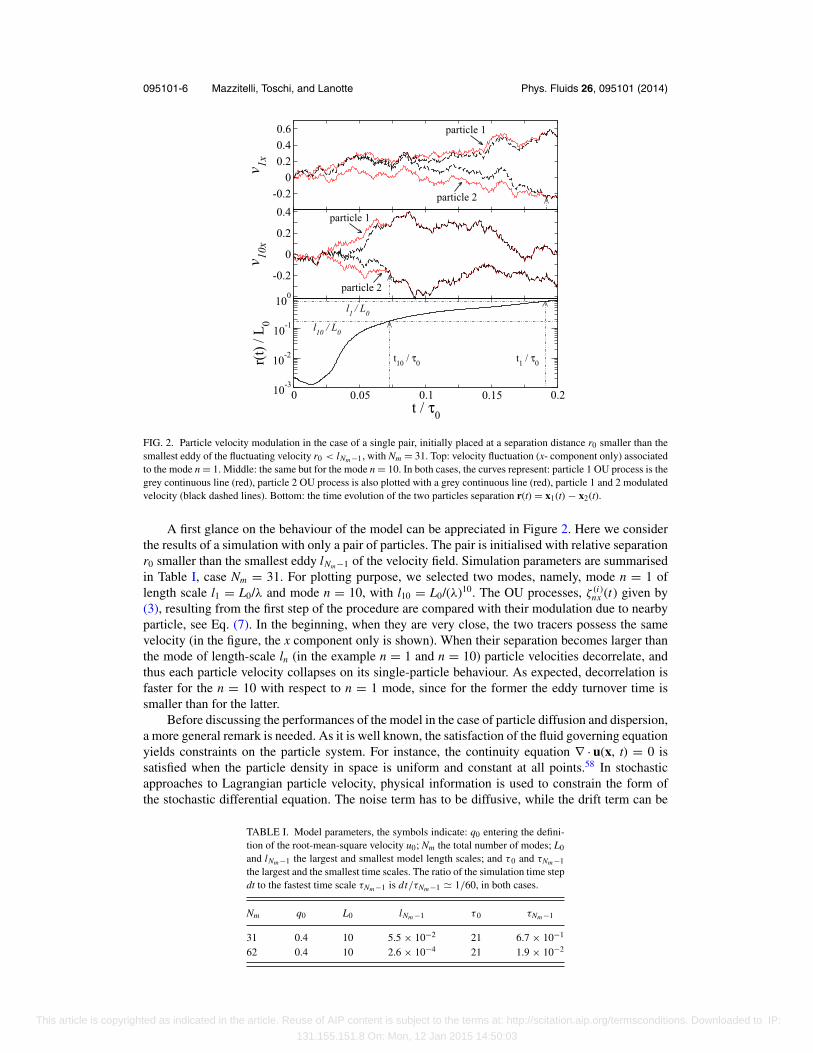
FIG. 2. Particle velocity modulation in the case of a single pair, initially placed at a separation distance r0 smaller than thesmallest eddy of the fluctuating velocity r0 < lNm−1, with Nm = 31. Top: velocity fluctuation (x- component only) associatedto the mode n = 1. Middle: the same but for the mode n = 10. In both cases, the curves represent: particle 1 OU process is thegrey continuous line (red), particle 2 OU process is also plotted with a grey continuous line (red), particle 1 and 2 modulatedvelocity (black dashed lines). Bottom: the time evolution of the two particles separation r(t) = x1(t) − x2(t).

A first glance on the behaviour of the model can be appreciated in Figure 2. Here we considerthe results of a simulation with only a pair of particles. The pair is initialised with relative separationr0 smaller than the smallest eddy lNm−1 of the velocity field. Simulation parameters are summarisedin Table I, case Nm = 31. For plotting purpose, we selected two modes, namely, mode n = 1 oflength scale l1 = L0/λ and mode n = 10, with l10 = L0/(λ)10. The OU processes, ζ (i)

nx (t) given by(3), resulting from the first step of the procedure are compared with their modulation due to nearbyparticle, see Eq. (7). In the beginning, when they are very close, the two tracers possess the samevelocity (in the figure, the x component only is shown). When their separation becomes larger thanthe mode of length-scale ln (in the example n = 1 and n = 10) particle velocities decorrelate, andthus each particle velocity collapses on its single-particle behaviour. As expected, decorrelation isfaster for the n = 10 with respect to n = 1 mode, since for the former the eddy turnover time issmaller than for the latter.

Before discussing the performances of the model in the case of particle diffusion and dispersion,a more general remark is needed. As it is well known, the satisfaction of the fluid governing equationyields constraints on the particle system. For instance, the continuity equation ∇ · u(x, t) = 0 issatisfied when the particle density in space is uniform and constant at all points.58 In stochasticapproaches to Lagrangian particle velocity, physical information is used to constrain the form ofthe stochastic differential equation. The noise term has to be diffusive, while the drift term can be

TABLE I. Model parameters, the symbols indicate: q0 entering the defini-tion of the root-mean-square velocity u0; Nm the total number of modes; L0

and lNm−1 the largest and smallest model length scales; and τ 0 and τNm−1

the largest and the smallest time scales. The ratio of the simulation time stepdt to the fastest time scale τNm−1 is dt/τNm−1 � 1/60, in both cases.

Nm q0 L0 lNm−1 τ 0 τNm−1

31 0.4 10 5.5 × 10−2 21 6.7 × 10−1

62 0.4 10 2.6 × 10−4 21 1.9 × 10−2

This article is copyrighted as indicated in the article. Reuse of AIP content is subject to the terms at: http://scitation.aip.org/termsconditions. Downloaded to IP:

131.155.151.8 On: Mon, 12 Jan 2015 14:50:03

095101-7 Mazzitelli, Toschi, and Lanotte Phys. Fluids 26, 095101 (2014)

specified on the basis of the Eulerian statistics of the flow. The physical request is that an initiallyuniform particle distribution will remain such, after Lagrangian evolution (from the Eulerian pointof view, a well-mixed scalar field remains so). In 3D there is no unique form for the drift term, butthere are a number of available solutions.40, 54

Tracer uniform distribution is clearly a crucial feature for a SGS model for incompressibleturbulence. In the Appendix, we discuss a series of tests we performed to assess the spatial distributionproperties of the Lagrangian tracers, or in other words to assess the incompressibility of the particlevelocity field.

III. RESULTS

We now discuss the results of two sets of numerical simulations, characterized by differentvalues of the total number of modes Nm, at fixed values of the integral scale L0 and root-mean-squarevelocity u0. Increasing the number of modes at fixed L0 and u0 results in an extension of the inertialrange of turbulence. For each set of numerical simulations, mean values are computed by ensembleaveraging over 50 simulations, each containing 100 particle pairs. Particles are initially uniformlydistributed in space, and such that the initial pair separation is smaller than the smallest eddy in thevelocity, lNm−1. Their total number is N = 104. The simulation parameters are reported in Table I.

We first consider the absolute dispersion, that is, the mean displacement of a single particlewith respect to its initial position. The statistical behaviour is expected to be ballistic for correlatedscales, followed by simple diffusion a la Taylor at scales larger than the velocity integral scale L0.To this aim we compute:

D(t) = 〈[x(t) − x(0)]2〉, (14)

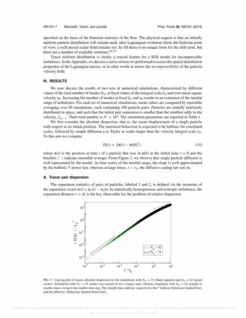
where x(t) is the position at time t of a particle that was in x(0) at the initial time t = 0 and thebrackets 〈 · 〉 indicate ensemble average. From Figure 3, we observe that single particle diffusion iswell represented by the model. At time scales of the inertial range, the slope is well approximatedby the ballistic t2 power law, whereas at large times, t > τ 0, the diffusive scaling law sets in.

A. Tracer pair dispersion

The separation statistics of pairs of particles, labeled 1 and 2, is defined via the moments ofthe separation vector r(t) = x1(t) − x2(t). In statistically homogeneous and isotropic turbulence, theseparation distance r = |r| is the key observable for the problem of relative dispersion.

10-4 10-3 10-2 10-1 100 101

t / τ0

10-6

10-4

10-2

100

102

< D

(t)

> / L

02

Nm = 62Nm = 31

FIG. 3. Log-log plot of tracers absolute dispersion for the simulations with Nm = 31 (black squares) and Nm = 62 (greencircles). Simulation with Nm = 31 modes was carried on for a longer time, whereas simulation with Nm = 62 extends tosmaller times, owing to the smaller time step. The straight lines indicate, respectively, the t2 ballistic behaviour (dashed line),and the diffusive t behaviour (dashed dotted line).

This article is copyrighted as indicated in the article. Reuse of AIP content is subject to the terms at: http://scitation.aip.org/termsconditions. Downloaded to IP:

131.155.151.8 On: Mon, 12 Jan 2015 14:50:03

095101-8 Mazzitelli, Toschi, and Lanotte Phys. Fluids 26, 095101 (2014)

10-4 10-3 10-2 10-1 100 101

t / τ0

10-8

10-6

10-4

10-2

100

102

< [ r

(t) -

r 0 ]2 > /

L 02

Nm = 62Nm = 31

t3

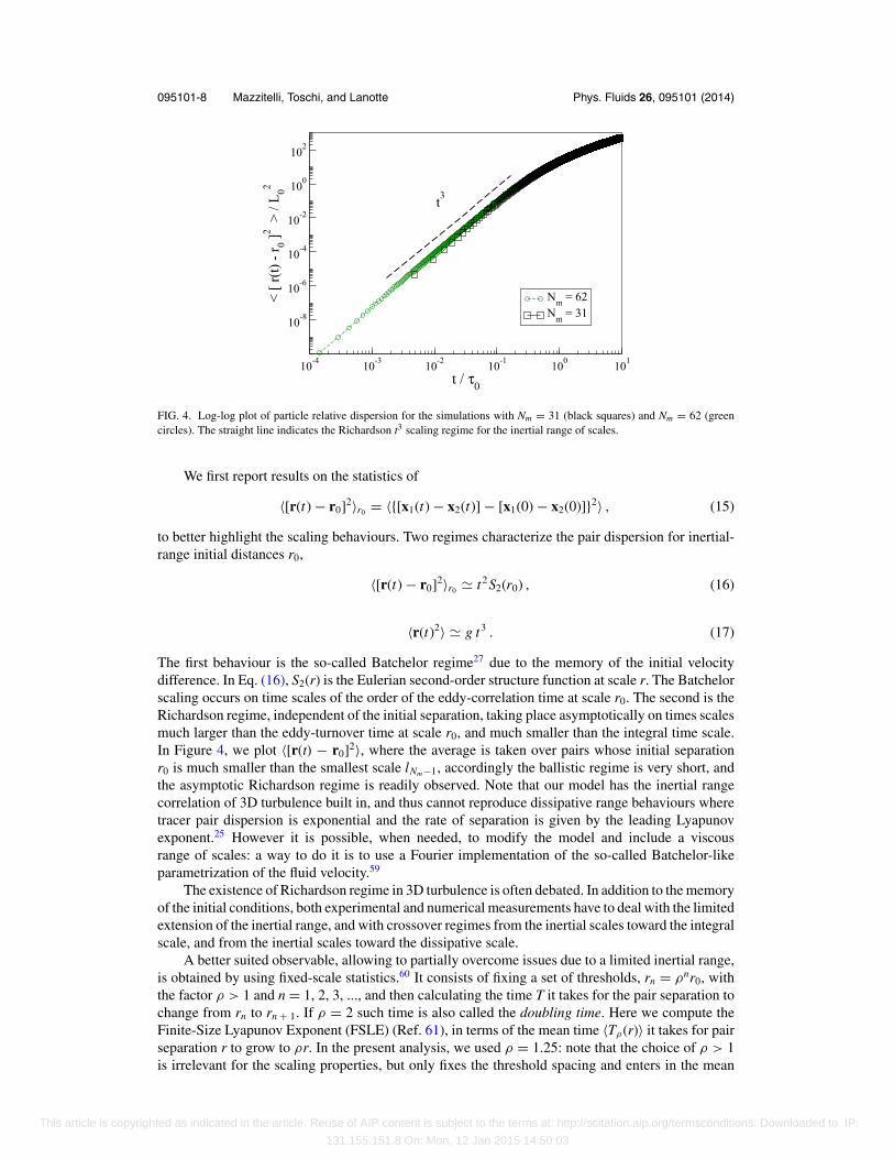
FIG. 4. Log-log plot of particle relative dispersion for the simulations with Nm = 31 (black squares) and Nm = 62 (greencircles). The straight line indicates the Richardson t3 scaling regime for the inertial range of scales.

We first report results on the statistics of

〈[r(t) − r0]2〉r0 = 〈{[x1(t) − x2(t)] − [x1(0) − x2(0)]}2〉 , (15)

to better highlight the scaling behaviours. Two regimes characterize the pair dispersion for inertial-range initial distances r0,

〈[r(t) − r0]2〉r0 � t2S2(r0) , (16)

〈r(t)2〉 � g t3 . (17)

The first behaviour is the so-called Batchelor regime27 due to the memory of the initial velocitydifference. In Eq. (16), S2(r) is the Eulerian second-order structure function at scale r. The Batchelorscaling occurs on time scales of the order of the eddy-correlation time at scale r0. The second is theRichardson regime, independent of the initial separation, taking place asymptotically on times scalesmuch larger than the eddy-turnover time at scale r0, and much smaller than the integral time scale.In Figure 4, we plot 〈[r(t) − r0]2〉, where the average is taken over pairs whose initial separationr0 is much smaller than the smallest scale lNm−1, accordingly the ballistic regime is very short, andthe asymptotic Richardson regime is readily observed. Note that our model has the inertial rangecorrelation of 3D turbulence built in, and thus cannot reproduce dissipative range behaviours wheretracer pair dispersion is exponential and the rate of separation is given by the leading Lyapunovexponent.25 However it is possible, when needed, to modify the model and include a viscousrange of scales: a way to do it is to use a Fourier implementation of the so-called Batchelor-likeparametrization of the fluid velocity.59

The existence of Richardson regime in 3D turbulence is often debated. In addition to the memoryof the initial conditions, both experimental and numerical measurements have to deal with the limitedextension of the inertial range, and with crossover regimes from the inertial scales toward the integralscale, and from the inertial scales toward the dissipative scale.

A better suited observable, allowing to partially overcome issues due to a limited inertial range,is obtained by using fixed-scale statistics.60 It consists of fixing a set of thresholds, rn = ρnr0, withthe factor ρ > 1 and n = 1, 2, 3, ..., and then calculating the time T it takes for the pair separation tochange from rn to rn + 1. If ρ = 2 such time is also called the doubling time. Here we compute theFinite-Size Lyapunov Exponent (FSLE) (Ref. 61), in terms of the mean time 〈Tρ(r)〉 it takes for pairseparation r to grow to ρr. In the present analysis, we used ρ = 1.25: note that the choice of ρ > 1is irrelevant for the scaling properties, but only fixes the threshold spacing and enters in the mean

This article is copyrighted as indicated in the article. Reuse of AIP content is subject to the terms at: http://scitation.aip.org/termsconditions. Downloaded to IP:

131.155.151.8 On: Mon, 12 Jan 2015 14:50:03

095101-9 Mazzitelli, Toschi, and Lanotte Phys. Fluids 26, 095101 (2014)

10-5 10-4 10-3 10-2 10-1 100 101

r / L0

10-2

10-1

100100

101

λ(r)

τ 0

Nm = 31Nm = 62

r-2/3

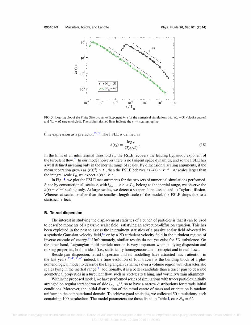
FIG. 5. Log-log plot of the Finite Size Lyapunov Exponent λ(r) for the numerical simulations with Nm = 31 (black squares)and Nm = 62 (green circles). The straight dashed lines indicate the r−2/3 scaling regime.

time expression as a prefactor.25, 62 The FSLE is defined as

λ(rn) = log ρ

〈Tρ(rn)〉 . (18)

In the limit of an infinitesimal threshold rn, the FSLE recovers the leading Lypanuov exponent ofthe turbulent flow.61 In our model however there is no tangent space dynamics, and so the FSLE hasa well defined meaning only in the inertial range of scales. By dimensional scaling arguments, if themean separation grows as 〈r(t)2〉 ∼ t3, then the FSLE behaves as λ(r) ∼ r−2/3. At scales larger thanthe integral scale L0, we expect λ(r) ∼ r−2.

In Fig. 5, we plot the FSLE measurements for the two sets of numerical simulations performed.Since by construction all scales r, with lNm−1 < r < L0, belong to the inertial range, we observe theλ(r) ∼ r−2/3 scaling only. At large scales, we detect a steeper slope, associated to Taylor diffusion.Whereas at scales smaller than the smallest length-scale of the model, the FSLE drops due to astatistical effect.

B. Tetrad dispersion

The interest in studying the displacement statistics of a bunch of particles is that it can be usedto describe moments of a passive scalar field, satisfying an advection-diffusion equation. This hasbeen exploited in the past to assess the intermittent statistics of a passive scalar field advected bya synthetic Gaussian velocity field,63 or by a 2D turbulent velocity field in the turbulent regime ofinverse cascade of energy.64 Unfortunately, similar results do not yet exist for 3D turbulence. Onthe other hand, Lagrangian multi-particle motion is very important when studying dispersion andmixing properties, both in ideal (i.e., statistically homogeneous and isotropic) and in real flows.

Beside pair dispersion, tetrad dispersion and its modelling have attracted much attention inthe last years:25, 43, 53, 65 indeed, the time evolution of four tracers is the building block of a phe-nomenological model to describe the Lagrangian dynamics over a volume region with characteristicscales lying in the inertial range;33 additionally, it is a better candidate than a tracer pair to describegeometrical properties in a turbulent flow, such as vortex stretching, and vorticity/strain alignment.

Within the proposed model, we have performed series of simulations with tracer particles initiallyarranged on regular tetrahedron of side lNm−1/2, so to have a narrow distributions for tetrads initialconditions. Moreover, the initial distribution of the tetrad centre of mass and orientation is randomuniform in the computational domain. To achieve good statistics, we collected 50 simulations, eachcontaining 100 tetrahedron. The model parameters are those listed in Table I, case Nm = 62.

This article is copyrighted as indicated in the article. Reuse of AIP content is subject to the terms at: http://scitation.aip.org/termsconditions. Downloaded to IP:

131.155.151.8 On: Mon, 12 Jan 2015 14:50:03

095101-10 Mazzitelli, Toschi, and Lanotte Phys. Fluids 26, 095101 (2014)

10-2

10-1

100

101

102

103

t / τNm-1

10-2

100

102

104

106

108

1010

< g

i > /

l 2 Nm

-1 t3

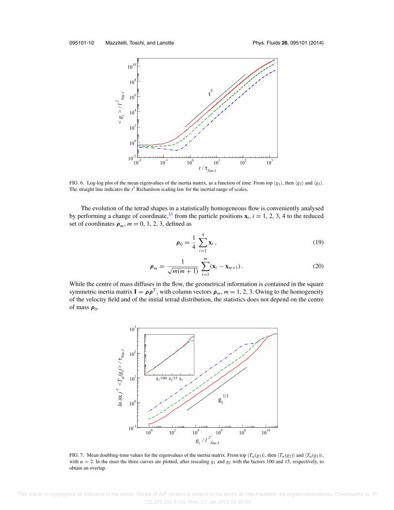
FIG. 6. Log-log plot of the mean eigenvalues of the inertia matrix, as a function of time. From top 〈g1〉, then 〈g2〉 and 〈g3〉.The straight line indicates the t3 Richardson scaling law for the inertial range of scales.

The evolution of the tetrad shapes in a statistically homogeneous flow is conveniently analysedby performing a change of coordinate,33 from the particle positions xi, i = 1, 2, 3, 4 to the reducedset of coordinates ρm , m = 0, 1, 2, 3, defined as

ρ0 = 1

4

4∑i=1

xi , (19)

ρm = 1√m(m + 1)

m∑i=1

(xi − xm+1) . (20)

While the centre of mass diffuses in the flow, the geometrical information is contained in the squaresymmetric inertia matrix I = ρρT , with column vectors ρm , m = 1, 2, 3. Owing to the homogeneityof the velocity field and of the initial tetrad distribution, the statistics does not depend on the centreof mass ρ0.

100

102

104

106

108

1010

gi / l

2

Nm-1

10-1

100

101

102

103

ln (

α )-1

<T

α(gi)>

/ τ N

m-1

g1/100 g

2/15 g

3

gi

1/3

FIG. 7. Mean doubling-time values for the eigenvalues of the inertia matrix. From top 〈Tα(g3)〉, then 〈Tα(g2)〉 and 〈Tα(g1)〉,with α = 2. In the inset the three curves are plotted, after rescaling g1 and g2 with the factors 100 and 15, respectively, toobtain an overlap.

This article is copyrighted as indicated in the article. Reuse of AIP content is subject to the terms at: http://scitation.aip.org/termsconditions. Downloaded to IP:

131.155.151.8 On: Mon, 12 Jan 2015 14:50:03

095101-11 Mazzitelli, Toschi, and Lanotte Phys. Fluids 26, 095101 (2014)

The matrix admits real positive eigenvalues, gi, that can be ordered according to: g1 ≥ g2 ≥ g3.The tetrahedron dimension is given by r = √

2/3 tr (I) = √2/3(g1 + g2 + g3) and the volume is

V = 1/3√

det(I) = 1/3√

g1g2g3. It is convenient to introduce the adimensional quantities Ii = gi/r2

(where I1 + I2 + I3 = 1), whose relative values give an indication of the tetrahedron shape. For aregular tetrahedron I1 = I2 = I3 = 1/3; when the four points are coplanar I3 = 0; when they arealigned I2 = I3 = 0.

We remark that by means of a stochastic model for tetrad dispersion, Devenish43 recentlyobtained values for the Ii indices in agreement with those of Direct Numerical Simulations of 3Dturbulence.

In Fig. 6, we present the temporal evolution of the mean eigenvalues of I. Numerical resultsshow good agreement with Richardson prediction, i.e., 〈gi〉 � t3. This issue is further verified bymeasuring fixed scale statistics. To this aim, we compute the average time 〈Tα(gi)〉 it takes for eacheigenvalue gi to increase its value of a factor α, with α = 2. Hence we measure the average doublingtimes of the eigenvalues gi, 〈Tα(gi)〉.

Results are plotted in Fig. 7. They indicate the existence of a wide inertial range, where theslope of the exit-time is g1/3

i , matching Richardson prediction.34 In addition, as shown in the inset,

10-2

100

102

t / τNm-1

0.0

0.2

0.4

0.6

0.8

1.0

< I

i >

10-1

100

101

102

103

t / τNm-1

0.0

0.2

0.4

0.6

0.8

1.0

< I

i >

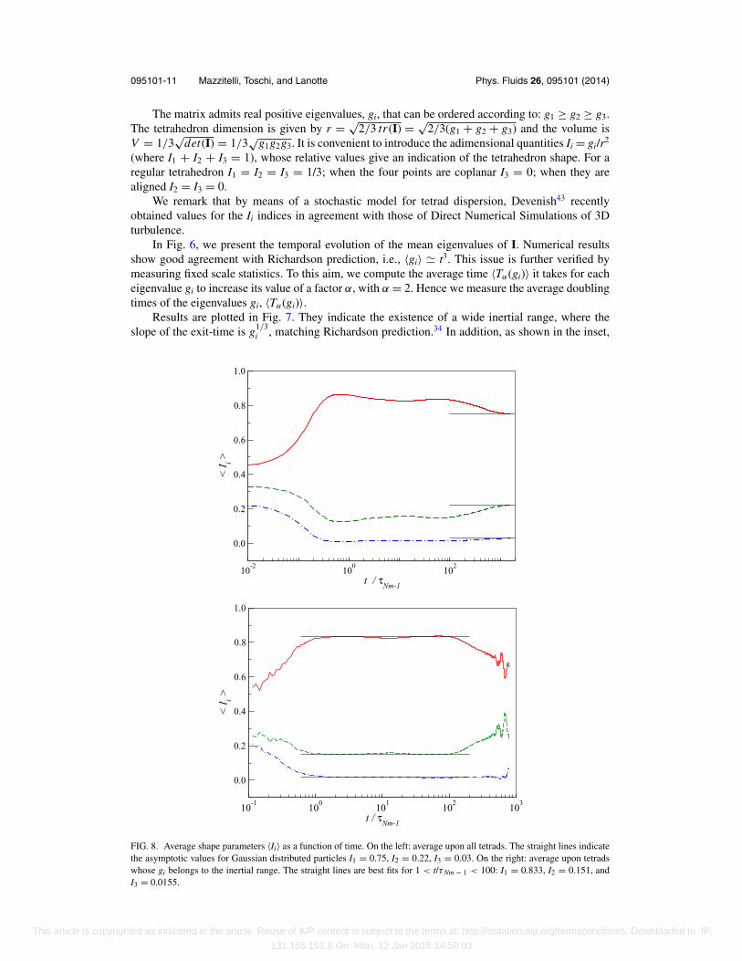
FIG. 8. Average shape parameters 〈Ii〉 as a function of time. On the left: average upon all tetrads. The straight lines indicatethe asymptotic values for Gaussian distributed particles I1 = 0.75, I2 = 0.22, I3 = 0.03. On the right: average upon tetradswhose gi belongs to the inertial range. The straight lines are best fits for 1 < t/τNm − 1 < 100: I1 = 0.833, I2 = 0.151, andI3 = 0.0155.

This article is copyrighted as indicated in the article. Reuse of AIP content is subject to the terms at: http://scitation.aip.org/termsconditions. Downloaded to IP:

131.155.151.8 On: Mon, 12 Jan 2015 14:50:03

095101-12 Mazzitelli, Toschi, and Lanotte Phys. Fluids 26, 095101 (2014)

the three eigenvalues overlap after rescaling g1 and g2 respectively with the factors 100 and 15.These scaling factors yield to I1 � 0.862, I2 � 0.129, I3 � 0.0086, i.e., on average very elongatedtetrahedra prevail.

The existence of a range where, after rescaling on the horizontal axis, the values of the doubling-times are the same for the three eigenvalues implies that the tetrads increase their dimension whilemaintaining the same (elongated) shape. These results can be compared with the DNS of Ref. 34.They show qualitative agreement, though the values of the rescaling factors applied to achieve theexit-times collapse are different.

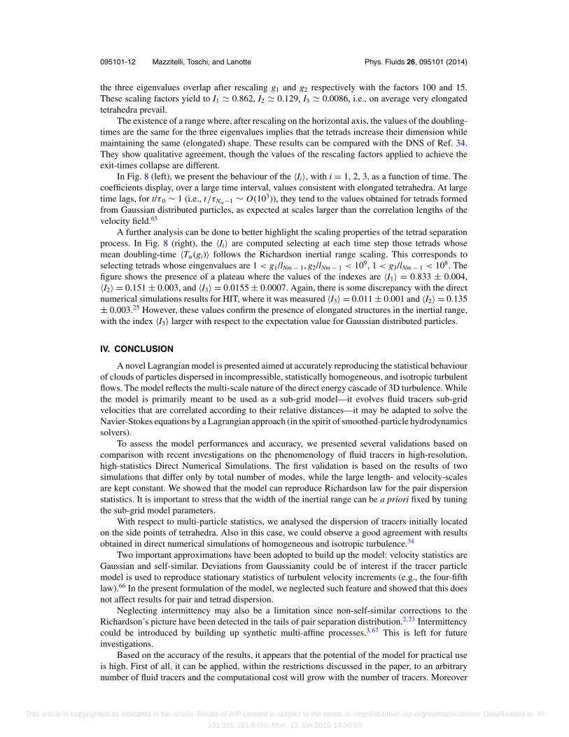
In Fig. 8 (left), we present the behaviour of the 〈Ii〉, with i = 1, 2, 3, as a function of time. Thecoefficients display, over a large time interval, values consistent with elongated tetrahedra. At largetime lags, for t/τ 0 ∼ 1 (i.e., t/τNm−1 ∼ O(103)), they tend to the values obtained for tetrads formedfrom Gaussian distributed particles, as expected at scales larger than the correlation lengths of thevelocity field.65

A further analysis can be done to better highlight the scaling properties of the tetrad separationprocess. In Fig. 8 (right), the 〈Ii〉 are computed selecting at each time step those tetrads whosemean doubling-time 〈Tα(gi)〉 follows the Richardson inertial range scaling. This corresponds toselecting tetrads whose eingenvalues are 1 < g1/lNm − 1, g2/lNm − 1 < 109, 1 < g3/lNm − 1 < 108. Thefigure shows the presence of a plateau where the values of the indexes are 〈I1〉 = 0.833 ± 0.004,〈I2〉 = 0.151 ± 0.003, and 〈I3〉 = 0.0155 ± 0.0007. Again, there is some discrepancy with the directnumerical simulations results for HIT, where it was measured 〈I3〉 = 0.011 ± 0.001 and 〈I2〉 = 0.135± 0.003.25 However, these values confirm the presence of elongated structures in the inertial range,with the index 〈I3〉 larger with respect to the expectation value for Gaussian distributed particles.

IV. CONCLUSION

A novel Lagrangian model is presented aimed at accurately reproducing the statistical behaviourof clouds of particles dispersed in incompressible, statistically homogeneous, and isotropic turbulentflows. The model reflects the multi-scale nature of the direct energy cascade of 3D turbulence. Whilethe model is primarily meant to be used as a sub-grid model—it evolves fluid tracers sub-gridvelocities that are correlated according to their relative distances—it may be adapted to solve theNavier-Stokes equations by a Lagrangian approach (in the spirit of smoothed-particle hydrodynamicssolvers).

To assess the model performances and accuracy, we presented several validations based oncomparison with recent investigations on the phenomenology of fluid tracers in high-resolution,high-statistics Direct Numerical Simulations. The first validation is based on the results of twosimulations that differ only by total number of modes, while the large length- and velocity-scalesare kept constant. We showed that the model can reproduce Richardson law for the pair dispersionstatistics. It is important to stress that the width of the inertial range can be a priori fixed by tuningthe sub-grid model parameters.

With respect to multi-particle statistics, we analysed the dispersion of tracers initially locatedon the side points of tetrahedra. Also in this case, we could observe a good agreement with resultsobtained in direct numerical simulations of homogeneous and isotropic turbulence.34

Two important approximations have been adopted to build up the model: velocity statistics areGaussian and self-similar. Deviations from Gaussianity could be of interest if the tracer particlemodel is used to reproduce stationary statistics of turbulent velocity increments (e.g., the four-fifthlaw).66 In the present formulation of the model, we neglected such feature and showed that this doesnot affect results for pair and tetrad dispersion.

Neglecting intermittency may also be a limitation since non-self-similar corrections to theRichardson’s picture have been detected in the tails of pair separation distribution.2, 23 Intermittencycould be introduced by building up synthetic multi-affine processes.3, 67 This is left for futureinvestigations.

Based on the accuracy of the results, it appears that the potential of the model for practical useis high. First of all, it can be applied, within the restrictions discussed in the paper, to an arbitrarynumber of fluid tracers and the computational cost will grow with the number of tracers. Moreover

This article is copyrighted as indicated in the article. Reuse of AIP content is subject to the terms at: http://scitation.aip.org/termsconditions. Downloaded to IP:

131.155.151.8 On: Mon, 12 Jan 2015 14:50:03

095101-13 Mazzitelli, Toschi, and Lanotte Phys. Fluids 26, 095101 (2014)

the model parameters can be chosen to achieve the desired extension of the inertial range. Finally,the absence of a grid makes the method suitable also for complex situations, for instance in thepresence of free surfaces. The capabilities of the model in more complex flows, e.g., shear andchannel flows, will be a matter of future investigations. Finally, the model may be easily modifiedto describe inertial heavy point-like particles.68

ACKNOWLEDGMENTS

We acknowledge useful discussions with Luca Biferale, Ben Devenish, and Guglielmo Lacorata.We acknowledge support from the EU COST Action MP0806. I.M.M. was supported by FIRB underGrant No. RBFR08QIP5_001. This work was partially supported by the Foundation for FundamentalResearch on Matter (FOM), a part of the Netherlands Organisation for Scientific Research (NWO).Numerical Simulations were performed on the Linux Cluster Socrate at CNR-ISAC (Lecce, Italy).We thank Dr. Fabio Grasso for technical support.

APPENDIX: PARTICLE SPATIAL DISTRIBUTION

In order to test particle model incompressibility, we performed the following experiment. Weseeded a periodic cubic domain withN = 1000 particles, uniformly distributed. The particle velocityfield has Nm = 31 velocity modes, that we followed for a few large eddy-turnover times, τ 0. Anuniform distribution of N particles in the volume V means that, after coarse-graining the volumein cells of size R, the number of particles in each cell, dubbed n(R), will be a random variable withPoisson distribution,

pR(n) = (λR)n

n!exp (−λR) . (A1)

Here λR = N /(L/R)3 is the average number of particles in a cell of size R3 and V = L3 is the totalvolume considered. From (A1), it is easy to derive

〈n2〉 = 〈n〉2 + 〈n〉. (A2)

Possible deviations from the uniform distribution can be systematically quantified, scale by scale, interms of the coefficient:

μ(R) = σ 2R

λ2R

= 〈n2〉 − 〈n〉2

〈n〉2, (A3)

where for a uniform distribution 〈n(R)〉 = λR = ρR3 and ρ = N /V is the particle number density,thus μ(R) = 1/(ρR3). Deviation from such behaviour can be also quantified in terms of the two-pointscorrelation in the particle distribution.

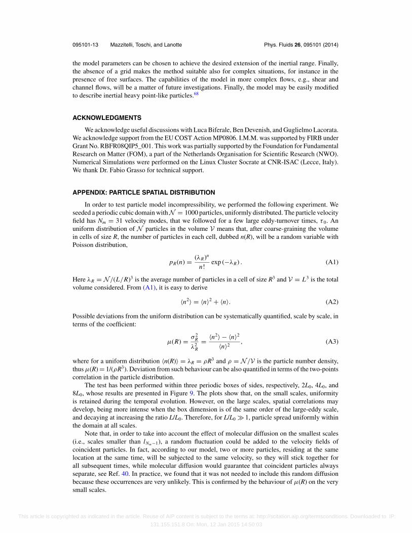
The test has been performed within three periodic boxes of sides, respectively, 2L0, 4L0, and8L0, whose results are presented in Figure 9. The plots show that, on the small scales, uniformityis retained during the temporal evolution. However, on the large scales, spatial correlations maydevelop, being more intense when the box dimension is of the same order of the large-eddy scale,and decaying at increasing the ratio L/L0. Therefore, for L/L0 � 1, particle spread uniformly withinthe domain at all scales.

Note that, in order to take into account the effect of molecular diffusion on the smallest scales(i.e., scales smaller than lNm−1), a random fluctuation could be added to the velocity fields ofcoincident particles. In fact, according to our model, two or more particles, residing at the samelocation at the same time, will be subjected to the same velocity, so they will stick together forall subsequent times, while molecular diffusion would guarantee that coincident particles alwaysseparate, see Ref. 40. In practice, we found that it was not needed to include this random diffusionbecause these occurrences are very unlikely. This is confirmed by the behaviour of μ(R) on the verysmall scales.

This article is copyrighted as indicated in the article. Reuse of AIP content is subject to the terms at: http://scitation.aip.org/termsconditions. Downloaded to IP:

131.155.151.8 On: Mon, 12 Jan 2015 14:50:03

095101-14 Mazzitelli, Toschi, and Lanotte Phys. Fluids 26, 095101 (2014)

FIG. 9. Coefficient μ(R) as a function of R/L for simulation with L = 2L0 (left), L = 4L0 (centre), and L = 8L0 (right).Results indicate: time t = 0 (black pluses), time t = 2τ 0 (red crosses), and the uniform distribution expectation, 1/(ρR3)(black straight line).

Results of Fig. 9 have a clear interpretation: particles tend to spread uniformly, but the velocitymodulation on the large scale induces spatial correlations. These can be further quantified andcontrolled according to the simple arguments that follows.

Starting from any initial spatial condition, when t > τ 0 the average distance of one particle toits closest neighbour, d1, can be estimated by the expression:69

d1 = 1

π1/2

[�

( D

2+ 1

)]1/D�

(1 + 1

D

)( VN

)1/D, (A4)

where � is the Euler Gamma function, D = 3 the space dimension, V the volume, and N thetotal number of particles. Numerical results agree with the theoretical expectation for randomlydistributed particles, Eq. (A4). The deviation of μ(R) from 1/(ρR3) occurs at a scale R ∼ d1 (i.e., R/L∼ 0.055 for N = 1000), because mode velocities on all scales larger than d1 are correlated. Clearly,the larger the number of correlated modes, the stronger the deviations from uniformity.

We remark that, when L0 = 10 and Nm = 31, there are 13 modes with length scale larger thand1 = 1.1 (average particle distance in simulations with L = 2L0) and only 5 modes with length scalelarger than d1 = 4.4 (average distance when L = 8L0). This explains the more intense deviationsdetected in the first plot of Figure 9 (first from the left), with respect to the third plot (third from theleft).

In general, the number of correlated modes Nc depends on the integral scale L0, on the modelparameter λ, and on the particle density ρ, according to

Nc = int

(1 + logλ

L0

d1

), (A5)

= int

(1 + logλ

( √π L0 ρ1/3

�(5/2)1/3 �(4/3)

)). (A6)

The average distance dn of a particle to its nth neighbour can also be computed. Recalling thatone point is the nth neighbor of another one if there are exactly n − 1 other points that are closer tothe latter than the former, the distance dn, in the case of N uniformly distributed particles, is:70

dn

L= 1

π1/2

[�(

D

2+ 1)

]1/D �(n + 1D )

�(n)

( 1

N)1/D

, (A7)

with the mean square fluctuation,(�dn

L

)2

= 1

π

[�(

D

2+ 1)

]2/D[

�(n + 2D )

�(n)− �2(n + 1

D )

�2(n)

] (1

N

)2/D

. (A8)

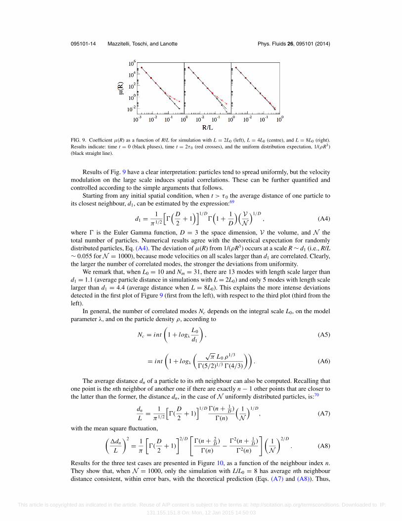
Results for the three test cases are presented in Figure 10, as a function of the neighbour index n.They show that, when N = 1000, only the simulation with L/L0 = 8 has average nth neighbourdistance consistent, within error bars, with the theoretical prediction (Eqs. (A7) and (A8)). Thus,

This article is copyrighted as indicated in the article. Reuse of AIP content is subject to the terms at: http://scitation.aip.org/termsconditions. Downloaded to IP:

131.155.151.8 On: Mon, 12 Jan 2015 14:50:03

095101-15 Mazzitelli, Toschi, and Lanotte Phys. Fluids 26, 095101 (2014)

FIG. 10. Average nth neighbour distance for n < 100. The curves represent: the theoretical expectation with error bars(cyan), simulation with L/L0 respectively equal to 8 (black pluses), 4 (green crosses), and 2 (red circles).

we infer that the ratio of correlated modes, Nc, to the total number of modes, Nm, has to be rathersmall in order for the model to satisfy incompressibility. The present indication is that Nc/Nm � 1/6is enough to produce uniformity at all scales (see Figure 9), with such a stringent test. When thepresent model is employed as a subgrid-scale Lagrangian model, this restriction can be relaxed asthe evolution on the larger scales will be matched with the resolved modes of the LES.

1 H. J. S. Fernando, D. Zajic, S. Di Sabatino, R. Dimitrova, B. Hedquist, and A. Dallman, “Flow, turbulence and pollutantdispersion in urban atmospheres,” Phys. Fluids 22, 051301 (2010).

2 R. Scatamacchia, L. Biferale, and F. Toschi, “Extreme events in the dispersions of two neighboring particles under theinfluence of fluid turbulence,” Phys. Rev. Lett. 109, 144501 (2012).

3 F. Toschi and E. Bodenschatz, “Lagrangian properties of particles in turbulence,” Annu. Rev. Fluid Mech. 41, 375 (2009).4 N. S. Holmes and L. Morawska, “Review of dispersion modelling and its application to the dispersion of particles: An

overview of different dispersion models available,” Atmos. Environ. 40, 5902 (2006).5 M. Chamecki and C. Meneveau, “Particle boundary layer above and downstream of an area source: Scaling, simulations,

and pollen transport,” J. Fluid Mech. 683, 1 (2011).6 G. Lacorata, A. Mazzino, and U. Rizza, “3D chaotic model for subgrid turbulent dispersion in large Eddy simulations,” J.

Atmos. Sci. 65(7), 2389 (2008).7 A. S. Lanotte and I. M. Mazzitelli, “Scalar turbulence in convective boundary layers by changing the entrainment flux,” J.

Atmos. Sci. 70, 248 (2013).8 S. Berti, F. A. Dos Santos, G. Lacorata, and A. Vulpiani, “Lagrangian drifter dispersion in the southwestern Atlantic ocean,”

J. Phys. Oceanogr. 41, 1659 (2011).9 L. Palatella, F. Bignami, F. Falcini, G. Lacorata, A. S. Lanotte, and R. Santoleri, “Lagrangian simulations and inter-annual

variability of anchovy egg and larva dispersal in the in the Sicily Channel,” J. Geophys. Res.: Oceans 119(2), 1306,doi:10.1002/2013JC009384 (2014).

10 R. A. Shaw, “Particle-turbulence interactions in atmospheric clouds,” Annu. Rev. Fluid Mech. 35, 183 (2003).11 M. U. Baebler, M. Morbidelli, and J. Badyga, “Modelling the breakup of solid aggregates in turbulent flows,” J. Fluid

Mech. 612, 261 (2008).12 M. U. Baebler, L. Biferale, and A. S. Lanotte, “Breakup of small aggregates driven by turbulent hydrodynamical stress,”

Phys. Rev. E 85, 025301(R) (2012).13 S. Post and J. Abraham, “Modeling the outcome of drop-drop collisions in Diesel sprays,” Int. J. Multiphase Flow 28, 997

(2002).14 P. Segaut, Large Eddy Simulation for Incompressible Flows, 3rd ed. (Springer, 2006).15 C. Meneveau and J. Katz, “Scale-invariance and turbulence models for large-Eddy simulation,” Annu. Rev. Fluid Mech.

32(1), 1 (2000).16 P. P. Sullivan, J. C. McWilliams, and C.-H. Moeng, “A sub-grid-scale model for large-eddy simulation of planetary

boundary layer flows,” Bound.-Layer Meteorol. 71, 247 (1994).17 E. Leveque, F. Toschi, L. Shao, and J.-P. Bertoglio, “Shear-improved Smagorinsky model for large-eddy simulation of

wall-bounded turbulent flows,” J. Fluid Mech. 570, 491 (2007).18 S. Ott and J. Mann, “An experimental investigation of the relative diffusion of particle pairs in three-dimensional turbulent

flows,” J. Fluid Mech. 422, 207 (2000).19 A. La Porta, G. A. Voth, A. M. Crawford, J. Alexander, and E. Bodenschatz, “Fluid particle accelerations in fully developed

turbulence,” Nature (London) 409, 1017 (2001).20 N. Mordant, P. Metz, O. Michel, and J. F. Pinton, “Measurement of Lagrangian velocity in fully developed turbulence,”

Phys. Rev. Lett. 87, 214501 (2001).

This article is copyrighted as indicated in the article. Reuse of AIP content is subject to the terms at: http://scitation.aip.org/termsconditions. Downloaded to IP:

131.155.151.8 On: Mon, 12 Jan 2015 14:50:03

095101-16 Mazzitelli, Toschi, and Lanotte Phys. Fluids 26, 095101 (2014)

21 T. Ishihara and Y. Kaneda, “Relative diffusion of a pair of fluid particles in the inertial subrange of turbulence,” Phys.Fluids 14(11), L69 (2002).

22 P. K. Yeung and M. S. Borgas, “Relative dispersion in isotropic turbulence: Part 1. Direct numerical simulations andReynolds number dependence,” J. Fluid Mech. 503, 125 (2004).

23 G. Boffetta and I. M. Sokolov, “Relative dispersion in fully developed turbulence: The Richardson’s law and intermittencycorrections,” Phys. Rev. Lett. 88, 094501 (2002).

24 L. Biferale, G. Boffetta, A. Celani, B. J. Devenish, A. Lanotte, and F. Toschi, “Multifractal statistics of Lagrangian velocityand acceleration in turbulence,” Phys. Rev. Lett. 93, 064502 (2004).

25 L. Biferale, G. Boffetta, A. Celani, B. J. Devenish, A. Lanotte, and F. Toschi, “Lagrangian statistics of particle pairs inhomogeneous isotropic turbulence,” Phys. Fluids 17, 115101 (2005).

26 P. K. Yeung, “Lagrangian investigations of turbulence,” Annu. Rev. Fluid Mech. 34, 115 (2002).27 B. Sawford, “Turbulent relative dispersion,” Annu. Rev. Fluid Mech. 33, 289 (2001).28 J. P. L. C. Salazar and L. R. Collins, “Two-particle dispersion in isotropic turbulent flows,” Annu. Rev. Fluid Mech. 41,

405 (2009).29 J. Bec, L. Biferale, A. S. Lanotte, A. Scagliarini, and F. Toschi, “Turbulent pair dispersion of inertial particles,” J. Fluid

Mech. 645, 497 (2010).30 J. C. Weil, P. P. Sullivan, and C.-H. Moeng, “The use of large-Eddy simulations in Lagrangian particle dispersion models,”

J. Atmos. Sci. 61, 2877 (2004).31 G. Jin and G.-W. He, “A nonlinear model for the subgrid timescale experienced by heavy particles in large eddy simulation

of isotropic turbulence with a stochastic differential equation,” New J. Phys. 15, 035011 (2013).32 G. Falkovich, K. Gawedzki, and M. Vergassola, “Particles and fields in fluid turbulence,” Rev. Mod. Phys. 73, 913 (2001).33 M. Chertkov, A. Pumir, and B. Shraiman, “Lagrangian tetrad dynamics and the phenomenology of turbulence,” Phys.

Fluids 11, 2394 (1999).34 L. Biferale, G. Boffetta, A. Celani, B. J. Devenish, A. Lanotte, and F. Toschi, “Multiparticle dispersion in fully developed

turbulence,” Phys. Fluids 17, 111701 (2005).35 H. Xu, N. T. Ouellette, and E. Bodenschatz, “Evolution of geometric structures in intense turbulence,” New J. Phys. 10,

013012 (2008).36 J. F. Hackl, P. K. Yeung, and B. L. Sawford, “Multi-particle and tetrad statistics in numerical simulations of turbulent

relative dispersion,” Phys. Fluids 23, 065103 (2011).37 A. Arneodo et al., “Universal intermittent properties of particle trajectories in highly turbulent flows,” Phys. Rev. Lett. 100,

254504 (2008).38 D. J. Thomson, “Criteria for the selection of stochastic models of particle trajectories in turbulent flows,” J. Fluid Mech.

180, 529 (1987).39 H. Kaplan and N. Dinar, “A three dimensional stochastic model for concentration fluctuation statistics in isotropic

homogeneous turbulence,” J. Comput. Phys. 79, 317 (1988).40 D. J. Thomson, “A stochastic model for the motion of particle pairs in isotropic high-Reynolds number turbulence, and its

application to the problem of concentration variance,” J. Fluid Mech. 210, 113 (1990).41 O. A. Kurbanmuradov, “Stochastic Lagrangian models for two-particle relative dispersion in high-Reynolds number

turbulence,” Monte Carlo Methods Appl. 3, 37 (1997).42 B. J. Devenish and D. J. Thomson, “A Lagrangian stochastic model for tetrad dispersion,” J. Turbul. 14(3), 107 (2013).43 B. J. Devenish, “Geometrical properties of turbulent dispersion,” Phys. Rev. Lett. 110, 064504 (2013).44 J. C. H. Fung, J. C. R. Hunt, N. A. Malik, and R. J. Perkins, “Kinematic simulation of homogeneous turbulent flows

generated by unsteady random Fourier modes,” J. Fluid Mech. 236, 281 (1992).45 J. C. H. Fung and J. C. Vassilicos, “Two-particle dispersion in turbulentlike flows,” Phys. Rev. E 57, 1677 (1998).46 M. Chaves, K. Gawedzki, P. Horvai, A. Kupiainen, and M. Vergassola, “Lagrangian dispersion in Gaussian self-similar

velocity ensembles,” J. Stat. Phys. 113, 643 (2003).47 D. J. Thomson and B. J. Devenish, “Particle pair separation in kinematic simulations,” J. Fluid Mech. 526, 277 (2005).48 G. L. Eyink and D. Benveniste, “Suppression of particle dispersion by sweeping effects in synthetic turbulence,” Phys.

Rev. E 87(2), 023011 (2013).49 J. G. M. Kuerten, “Subgrid modeling in particle-laden channel flow,” Phys. Fluids 18, 025108 (2006).50 C. Marchioli, M. V. Salvetti, and A. Soldati, “Some issues concerning large-Eddy simulation of inertial particle dispersion

in turbulent bounded flows,” Phys. Fluids 20, 040603 (2008).51 E. Calzavarini, A. Donini, V. Lavezzo, C. Marchioli, E. Pitton, A. Soldati, and F. Toschi, “On the error estimate in sub-grid

models for particles in turbulent flows,” in Direct and Large-Eddy Simulation VIII, ERCOFTAC Series Vol. 15 (Springer,Netherlands, 2011), 171–176.

52 J. J. Monaghan, “Smoothed particle hydrodynamics and its diverse applications,” Annu. Rev. Fluid Mech. 44, 323 (2012).53 B. L. Sawford, S. B. Pope, and P. K. Yeung, “Gaussian Lagrangian stochastic models for multi-particle dispersion,” Phys.

Fluids 25, 055101 (2013).54 M. S. Borgas and B. L. Sawford, “A family of stochastic models for two-particle dispersion in isotropic homogeneous

stationary turbulence,” J. Fluid Mech. 279, 69 (1994).55 T. Burgener, D. Kadau, and H. Herrmann, “Particle and particle pair dispersion in turbulence modeled with spatially and

temporally correlated stochastic processes,” Phys. Rev. E 86, 046308 (2012).56 U. Frisch, Turbulence: The legacy of A. N. Kolmogorov (Cambridge University Press, New York, 1995).57 D. T. Gillespie, “Exact numerical simulation of the Ornstein-Uhlenbeck process and its integral,” Phys. Rev. E 54, 2084

(1996).58 S. B. Pope, Turbulent Flows (Cambridge University Press, 2000).59 C. Meneveau, “Transition between viscous and inertial-range scaling of turbulence structure functions,” Phys. Rev. E 54,

3657 (1996).

This article is copyrighted as indicated in the article. Reuse of AIP content is subject to the terms at: http://scitation.aip.org/termsconditions. Downloaded to IP:

131.155.151.8 On: Mon, 12 Jan 2015 14:50:03

095101-17 Mazzitelli, Toschi, and Lanotte Phys. Fluids 26, 095101 (2014)

60 V. Artale, G. Boffetta, A. Celani, M. Cencini, and A. Vulpiani, “Dispersion of passive tracers in closed basins: Beyond thediffusion coefficient,” Phys. Fluids 9, 3162 (1997).

61 M. Cencini and A. Vulpiani, “Finite size Lyapunov exponent: Review on applications,” J. Phys. A: Math. Theor. 46, 254019(2013).

62 G. Boffetta and I. M. Sokolov, “Statistics of two-particle dispersion in two-dimensional turbulence,” Phys. Fluids 14, 3224(2002).

63 U. Frisch, A. Mazzino, and M. Vergassola, “Intermittency in passive scalar advection,” Phys. Rev. Lett. 80, 5532 (1998).64 A. Celani and M. Vergassola, “Statistical geometry in scalar turbulence,” Phys. Rev. Lett. 86(3), 424 (2001).65 A. Pumir, B. I. Shraiman, and M. Chertkov, “Geometry of Lagrangian dispersion in turbulence,” Phys. Rev. Lett. 85, 5324

(2000).66 G. Pagnini, “Lagrangian stochastic models for turbulent relative dispersion based on particle pair rotation,” J. Fluid Mech.

616, 357 (2008).67 L. Biferale, G. Boffetta, A. Celani, A. Crisanti, and A. Vulpiani, “Mimicking a turbulent signal: Sequential multiaffine

processes,” Phys. Rev. E 57(6), R6261 (1998).68 M. R. Maxey and J. Riley, “Equation of motion of a small rigid sphere in a nonuniform flow,” Phys. Fluids 26, 883 (1983).69 S. Chandrasekhar, “Stochastic problems in physics and astronomy,” Rev. Mod. Phys. 15, 1 (1943).70 A. G. Percus and O. C. Martin, “Finite size and dimensional dependence in the Euclidean traveling salesman problem,”

Phys. Rev. Lett. 76, 1188 (1996).

This article is copyrighted as indicated in the article. Reuse of AIP content is subject to the terms at: http://scitation.aip.org/termsconditions. Downloaded to IP:

131.155.151.8 On: Mon, 12 Jan 2015 14:50:03