An Accounting Exercise for the Shift in Life-Cycle

Employment Profiles of Married Women Born

Between 1940 and 1960

Sebastien Buttet and Alice Schoonbroodt∗

September 30, 2006

Abstract

Life-cycle employment profiles of married women born between 1940 and 1960

shifted upwards and became flatter. We calibrate a dynamic life-cycle model of

employment decisions of married women to assess the quantitative importance of

three competing explanations of the change in employment profiles: the decrease

and delay in fertility, the increase in relative wages of women to men, and the

decline in child-care costs. We find that the decrease and delay in fertility and the

decline in child-care cost affect employment very early in life, while increases in

relative wages affect employment increasingly with age. Changes in relative wages,

∗Cleveland State University and University of Southampton. We thank Michele Boldrin, and Larry

Jones for their support and advice. We have benefitted a lot from discussions with Stefania Albanesi, My-

ong Chang, V.V. Chari, Zvi Eckstein, Alessandra Fogli, Mikhail Golosov, Jeremy Greenwood, Claudia

Olivetti, Ellen McGrattan, B. RaviKumar, Michele Tertilt, participants at the Midwest Macro Con-

ference 2005, SITE 2005, and Vienna Macro Workshop 2005. All errors are ours. Correspondence:

alicesch@soton.ac.uk or s.buttet@csuohio.edu.

1

in particular returns to experience, account for the bulk (67 percent) of changes in

life-cycle employment of married women.

1 Introduction

In the United States, as well as in many other developed countries, life-cycle employment

profiles of married women born around mid-century changed in a noticeable way. Em-

ployment rates of women born in 1940 and earlier are low at childbearing ages (between

age 20 to 35) and increase over the life-cycle. Changes in employment across cohorts are

not uniform along the life-cycle, however. They are very pronounced at childbearing ages

and more modest at later ages. As a result, life-cycle employment profiles of women born

in 1960 not only shift upwards but also become much flatter.

In this paper, we build a dynamic life-cycle model of employment decisions of married

women to assess the quantitative importance of three competing explanations of the

change in life-cycle employment profiles: the decrease and delay in fertility, the increase

in relative wages of women to men, and the decline in child-care costs. The incentives at

work are not new. First, because child-rearing is intensive in women’s time, employment

at childbearing ages increases as fertility is reduced. Second, postponing fertility allows

women to reach childbearing ages with a higher stock of accumulated work experience,

thereby increasing their incentives to remain employed when having children. Finally,

either an increase in women’s wages relative to men or a decline in the cost of child-care

makes working more attractive at childbearing ages, which feeds back on employment

decisions later on in life because of experience accumulation.

After calibrating the model to the life-cycle facts characterizing the 1940 cohort, we

show that the decrease and delay in fertility and the decline in child-care cost affect

employment very early in life, while increases in relative wages affect employment in-

creasingly with age. Assuming that the three forces account for 100 percent of the shift

2

in life-cycle employment profiles, we find that changes in women’s wages (in particular,

returns to experience) account for 67 percent of the increase, versus 22 percent for cost

of child-care, and 9 percent for fertility patterns (the residual term is equal to 2 percent).

The effects of decrease and delay in fertility offset each other. Employment rates tend to

increase following a decrease in fertility since reservation rates increase with the number

of children. However, because of the presence of young children in the household, a delay

in the timing of births tends to decrease fertility at later ages, since young children are

more costly.

Our calibration procedure is new, as dynamic life-cycle models of employment deci-

sions of married women are often estimated using maximum likelihood techniques (e.g.,

Eckstein and Wolpin 1989, Van der Klauuw 1996, or Francesconi 2002, to name only a

few papers). Maximum likelihood is a more refined statistical procedure since it takes

into account higher order moments, while we only match the average employment along

the life-cycle.1 Since large panel data sets are not available yet for the early cohorts we

consider, we use a sequence of cross-sectional data from the Current Population Survey

(CPS) from 1962 to 2004. Hence, we do not have all the information necessary to perform

the maximum likelihood (i.e., conditional means and variances). We believe that calibrat-

ing the model is appropriate for the question at hand and find that it yields surprisingly

good results. We obtain a very tight fit not only for the entire life-cycle employment

profile of the 1940 cohort, but also for the employment by number of children at various

ages. Moreover, we conduct sensitivity analysis to assess the robustness of our choice of

parameter values.

The contribution of our accounting exercise is clear. Three influential papers have

stressed the importance of changes in the pure gender wage gap (Jones, Manuelli, and

McGrattan 2003), changes in returns to experience (Olivetti 2006), and changes in child-

1See Schoonbroodt (2002) and Eckstein and van der Berg (2005) for advantages and disadvantages of

maximum likelihood versus moments estimation.

3

care costs relative to life-time earnings (Attanasio, Low, and Sanchez-Marcos 2004) to

account for changes in women’s labor supply either over time or across cohorts. Since our

model nests these three potential explanations and adds another one (the decrease and

delay in fertility), we can assess the quantitative importance of each of these forces sepa-

rately. We find that they affect employment of women in distinct age groups differently

and that changes in returns to experience have the largest impact on women’s employ-

ment. Moreover, we show that a careful modeling of the distributions for number and

timing of births is fruitful. First, it allows us to match the entire life-cycle employment of

married women born in 1940. Second, once we control for changes in fertility patterns, ex-

ogenous changes in women’s wages and cost of children that are needed to match changes

in employment across cohorts are smaller in magnitude compared to the ones found in

Jones, Manuelli, and McGrattan (2003) for the gender wage gap, Olivetti (2006) for re-

turns to experience, and Attanasio, Low, and Sanchez-Marcos (2004) for decreases in the

cost of child-care.

Numerous other explanations for the increase in employment of married women, either

over time or across cohorts, have been proposed. These include falling prices of home

appliances (Greenwood, Seshadri, and Yorukoglu 2005), changes in the perceived value

of marriage (Caucutt, Guner, and Knowles 2002), the introduction of the pill (Goldin

and Katz 2002), changes in social norms (Fernandes, Fogli, and Olivetti 2004), or gender-

biased technological change favoring women (Galor and Weil 1996), to name only a few.

These papers are certainly important. However, it is virtually impossible, let alone not

desirable, to include all of the aforementioned forces into one single model. To perform

our accounting exercise, we chose the ones which could be modeled without too much

controversy and seemed the most likely to influence women’s employment decisions at

childbearing ages.

The paper is built as follows. In Section 2, we present evidence for the change in

4

life-cycle patterns of employment and fertility for two cohorts of married women born in

the United States in 1940 and 1960. In Section 3, we describe a dynamic life-cycle model

of employment decisions of married women with experience accumulation. In Section 4,

we explain our procedure for the calibration of the model. In Section 5, we perform the

accounting exercise and, finally, we provide some concluding remarks in Section 6.

2 Data

We use data from the Current Population Survey (CPS) for the survey years 1964-2003

and from the decennial Census for the survey years 1970-2000 to describe the life-cycle

patterns of employment and fertility for two cohorts of married women born in the United

States in 1940 and 1960.2

2.1 Employment

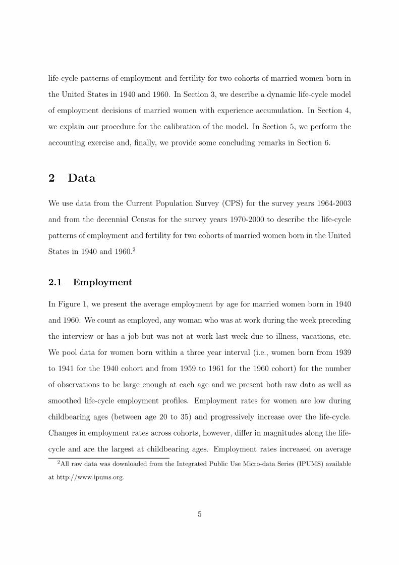
In Figure 1, we present the average employment by age for married women born in 1940

and 1960. We count as employed, any woman who was at work during the week preceding

the interview or has a job but was not at work last week due to illness, vacations, etc.

We pool data for women born within a three year interval (i.e., women born from 1939

to 1941 for the 1940 cohort and from 1959 to 1961 for the 1960 cohort) for the number

of observations to be large enough at each age and we present both raw data as well as

smoothed life-cycle employment profiles. Employment rates for women are low during

childbearing ages (between age 20 to 35) and progressively increase over the life-cycle.

Changes in employment rates across cohorts, however, differ in magnitudes along the life-

cycle and are the largest at childbearing ages. Employment rates increased on average

2All raw data was downloaded from the Integrated Public Use Micro-data Series (IPUMS) available

at http://www.ipums.org.

5

by 24 percentage points between age 20 and 35, compared to only 11 percentage points

between age 36 and 50 (see Table 1). This fact is the focus of our analysis.3

Fig. 1: Life-Cycle Employment Profile of Married Women by Cohort

20 25 30 35 40 45 500

0.1

0.2

0.3

0.4

0.5

0.6

0.7

0.8

0.9

1

Age

Par

ticip

atio

nBorn in 19401960

Tab. 1: Employment Rates of Married Women by Cohort and

Age Group

Age 20-35 a Age 36-50 b Age 20-50 c,d

1940 Cohort 37 62 52

1960 Cohort 61 73 65

Change (in pct. points) +24 +11 +13

aAge 24-35 for 1940 cohort. bAge 36-43 for 1960 cohort. cAge 24-50

for 1940 cohort. dAge 20-43 for 1960 cohort.

3In the Appendix, we show that increases in employment rates are the largest at childbearing ages

throughout the education ladder. As a result, the increase in the fraction of women with a college degree

can only account for a small fraction of the increase in women’s employment across cohorts.

6

2.2 Fertility

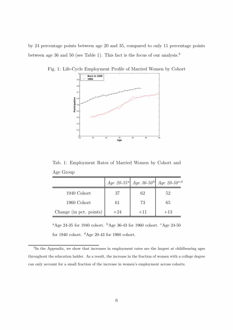
We use Census data for the years between 1980 and 2000 to describe the distributions

for the total number of children ever born and the age of mother at birth of first child of

married women born in 1940 and 1960. We consider married women at age 40, assuming

that fertility is close to completion at that age, and record the fraction with 0, 1,..., 4+

children, where 4+ denotes married women with at least 4 children. On average, women

born in 1940 had 2.6 children by age 40, while those born in 1960 had 1.9 (see Table 2).

Moreover, the decrease in the total number of children ever born mainly occurred from

a redistribution of mass away from 3 and 4 children towards 0, 1, and 2 children (see

Figure 2).

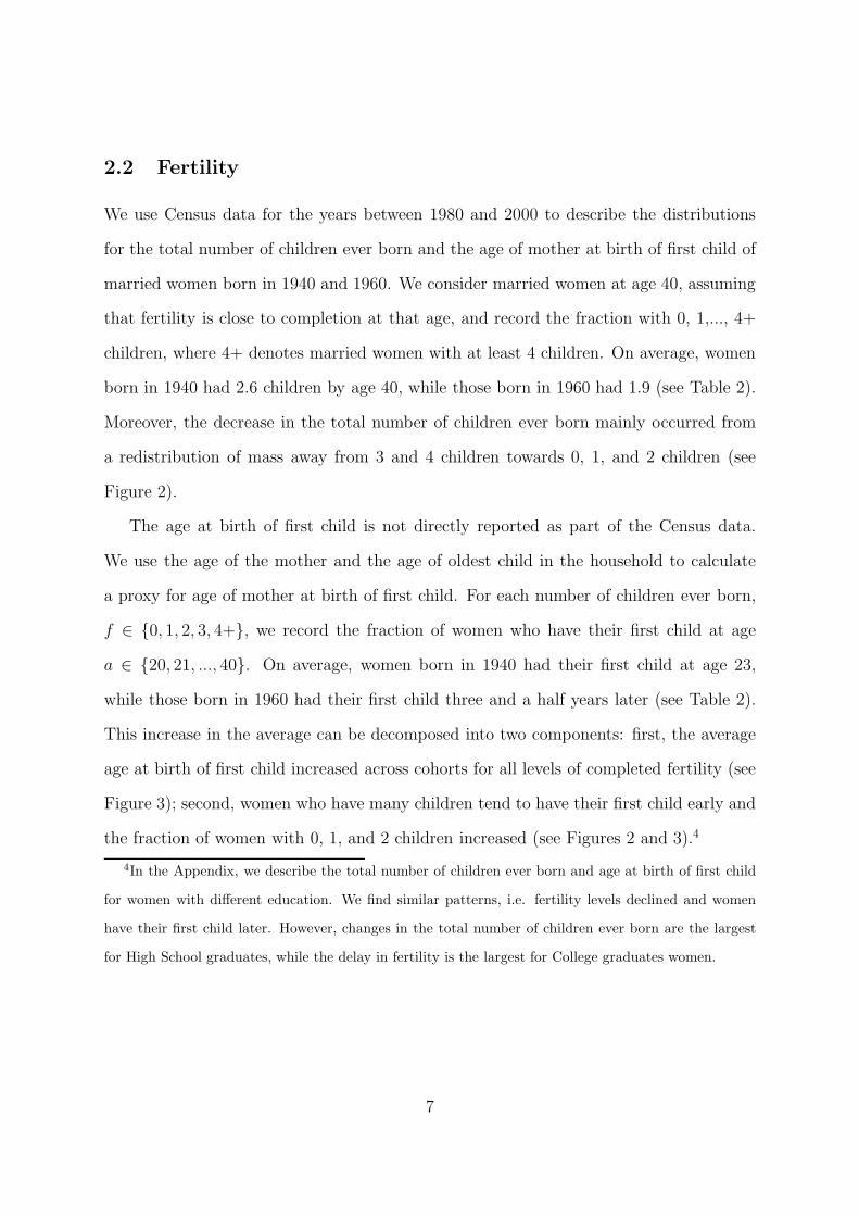
The age at birth of first child is not directly reported as part of the Census data.

We use the age of the mother and the age of oldest child in the household to calculate

a proxy for age of mother at birth of first child. For each number of children ever born,

f ∈ {0, 1, 2, 3, 4+}, we record the fraction of women who have their first child at age

a ∈ {20, 21, ..., 40}. On average, women born in 1940 had their first child at age 23,

while those born in 1960 had their first child three and a half years later (see Table 2).

This increase in the average can be decomposed into two components: first, the average

age at birth of first child increased across cohorts for all levels of completed fertility (see

Figure 3); second, women who have many children tend to have their first child early and

the fraction of women with 0, 1, and 2 children increased (see Figures 2 and 3).4

4In the Appendix, we describe the total number of children ever born and age at birth of first child

for women with different education. We find similar patterns, i.e. fertility levels declined and women

have their first child later. However, changes in the total number of children ever born are the largest

for High School graduates, while the delay in fertility is the largest for College graduates women.

7

Tab. 2: Fertility Levels and Timing of Births by Cohort - (Std. Dev.)

Cohort 1940 Cohort 1960

Total Number of Children Ever Born : 2.6 (1.2) 1.9 (1.1)

Age of Mother at Birth of First Child: 23.2 (2.9) 26.7 (4.7)

Fig. 2: Completed Fertility by Cohort

0 1 2 3 40

0.05

0.1

0.15

0.2

0.25

0.3

0.35

0.4

0.45

Number of Children Ever Born

Mean = 2.6Mean = 1.9

1940 Cohort

1960 Cohort

Fig. 3: Timing of Births by Completed Fertility and Cohort

15 20 25 30 35 40 450

0.05

0.1

0.15

Age

1 Child

15 20 25 30 35 40 450

0.05

0.1

0.15

Age

2 Children

15 20 25 30 35 40 450

0.05

0.1

0.15

Age

3 Children

15 20 25 30 35 40 450

0.05

0.1

0.15

Age

4 Children

19401960

8

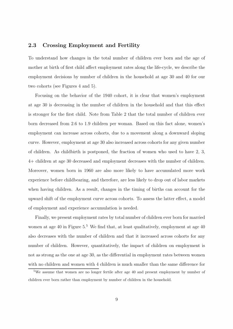
2.3 Crossing Employment and Fertility

To understand how changes in the total number of children ever born and the age of

mother at birth of first child affect employment rates along the life-cycle, we describe the

employment decisions by number of children in the household at age 30 and 40 for our

two cohorts (see Figures 4 and 5).

Focusing on the behavior of the 1940 cohort, it is clear that women’s employment

at age 30 is decreasing in the number of children in the household and that this effect

is stronger for the first child. Note from Table 2 that the total number of children ever

born decreased from 2.6 to 1.9 children per woman. Based on this fact alone, women’s

employment can increase across cohorts, due to a movement along a downward sloping

curve. However, employment at age 30 also increased across cohorts for any given number

of children. As childbirth is postponed, the fraction of women who used to have 2, 3,

4+ children at age 30 decreased and employment decreases with the number of children.

Moreover, women born in 1960 are also more likely to have accumulated more work

experience before childbearing, and therefore, are less likely to drop out of labor markets

when having children. As a result, changes in the timing of births can account for the

upward shift of the employment curve across cohorts. To assess the latter effect, a model

of employment and experience accumulation is needed.

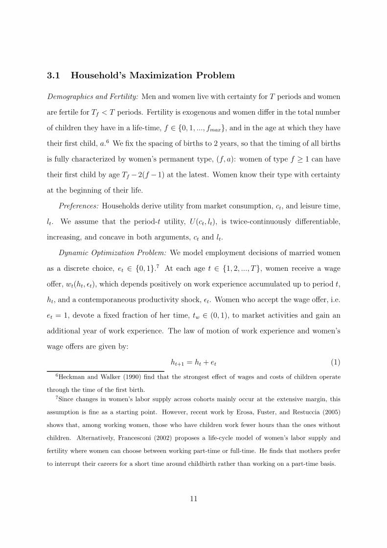
Finally, we present employment rates by total number of children ever born for married

women at age 40 in Figure 5.5 We find that, at least qualitatively, employment at age 40

also decreases with the number of children and that it increased across cohorts for any

number of children. However, quantitatively, the impact of children on employment is

not as strong as the one at age 30, as the differential in employment rates between women

with no children and women with 4 children is much smaller than the same difference for

5We assume that women are no longer fertile after age 40 and present employment by number of

children ever born rather than employment by number of children in the household.

9

Fig. 4: Employment of Married Women at Age 30 by Number of Children and Cohort

0 1 2 3 4+0

0.1

0.2

0.3

0.4

0.5

0.6

0.7

0.8

0.9

1

Number of Children in the Household

Par

ticip

atio

n

1940 Cohort1960 Cohort

Fig. 5: Employment of Married Women at Age 40 by Number of Children and Cohort

0 1 2 3 4+0

0.1

0.2

0.3

0.4

0.5

0.6

0.7

0.8

0.9

1

Number of Children Ever Born

Par

ticip

atio

n

1940 Cohort1960 Cohort

women at age 30.

3 A Life-Cycle Model

In this section, we build the aforementioned economic mechanisms into a life-cycle model

of employment decisions of married women with heterogenous agents and experience

accumulation. Our model is close to Eckstein and Wolpin (1989).

10

3.1 Household’s Maximization Problem

Demographics and Fertility: Men and women live with certainty for T periods and women

are fertile for Tf < T periods. Fertility is exogenous and women differ in the total number

of children they have in a life-time, f ∈ {0, 1, ..., fmax}, and in the age at which they have

their first child, a.6 We fix the spacing of births to 2 years, so that the timing of all births

is fully characterized by women’s permanent type, (f, a): women of type f ≥ 1 can have

their first child by age Tf −2(f −1) at the latest. Women know their type with certainty

at the beginning of their life.

Preferences: Households derive utility from market consumption, ct, and leisure time,

lt. We assume that the period-t utility, U(ct, lt), is twice-continuously differentiable,

increasing, and concave in both arguments, ct and lt.

Dynamic Optimization Problem: We model employment decisions of married women

as a discrete choice, et ∈ {0, 1}.7 At each age t ∈ {1, 2, ..., T}, women receive a wage

offer, wt(ht, ǫt), which depends positively on work experience accumulated up to period t,

ht, and a contemporaneous productivity shock, ǫt. Women who accept the wage offer, i.e.

et = 1, devote a fixed fraction of her time, tw ∈ (0, 1), to market activities and gain an

additional year of work experience. The law of motion of work experience and women’s

wage offers are given by:

ht+1 = ht + et (1)

6Heckman and Walker (1990) find that the strongest effect of wages and costs of children operate

through the time of the first birth.7Since changes in women’s labor supply across cohorts mainly occur at the extensive margin, this

assumption is fine as a starting point. However, recent work by Erosa, Fuster, and Restuccia (2005)

shows that, among working women, those who have children work fewer hours than the ones without

children. Alternatively, Francesconi (2002) proposes a life-cycle model of women’s labor supply and

fertility where women can choose between working part-time or full-time. He finds that mothers prefer

to interrupt their careers for a short time around childbirth rather than working on a part-time basis.

11

and

ln(wt(ht, ǫt)) = β0 + β1ht + β2h2t + ǫt (2)

where ǫt is normally distributed with mean 0 and standard deviation, σ2ǫ , and is i.i.d.

over time.8 We do not model joint participation decisions between husbands and wives.

Men work with certainty in each period and their (deterministic) wage in period t is

equal to wmt.9 Given the time discount factor, δ ∈ (0, 1), women of type (f, a) choose

employment, et, to maximize the expected discounted utility, Et−1

∑T

s=t δs−tU(cs, ls),

subject to a sequence of budget and time constraints and the law of motion for work

experience. In period t, the budget and time constraints are given by:

ct + g(f, a, et) ≤ wmt + wt(ht, ǫt)et

lt + ettw + t(f, a, et) = 1

et ∈ {0, 1}

(3)

where the time-invariant functions, g(·, ·, ·) and t(·, ·, ·), denote the goods and time cost of

children, respectively. Notice that we model the costs of children carefully, allowing them

to depend on the age of children and women’s participation choices. Following the work

of Hotz and Miller (1988), we assume that both functions are increasing in the number

of children and decreasing in age of children. On the other hand, goods costs increase

8The i.i.d assumption considerably reduces the dimension of the state space since we only need to

keep track the current productivity shock as opposed to the entire history of shocks. In recent work,

Meghir and Pistaferri (2004) and Guvenen (2005) reject the hypothesis that men’s wage shocks are i.i.d

over time and find strong empirical support for permanent and transitory wage shocks. However, since

work experience is endogenous in our model, women’s wages are serially correlated across periods even

though productivity shocks are i.i.d.. Note that, if the woman works every period, work experience

coincides with age and equation (2) boils down to a simple Mincer equation.9Husband’s wages are realized only after women’s participation is made in Eckstein and Wolpin (1989)

or Van der Klaauw (1996). Since they assume that utility is linear in consumption, women’s participation

decisions depend on husband’s expected income.

12

with participation, while time costs decrease. This reflects the necessity of some sort of

child-care when the woman works.

Our model abstracts from three important features. First, households cannot borrow

or lend, implying that the only way to smooth consumption over the life-cycle is through

women’s labor supply.10 Second, there is no depreciation in skills when women drop

out of labor markets and only the stock of accumulated work experience, as opposed

to the entire history of past employment decisions, matters to determine the average

wage offers. Although these assumptions considerably reduce the dimension for the state

space, Altug and Miller (1998) show that recent work experience is more valuable than

distant one to determine women’s wage offers. Finally, there are no permanent differ-

ences in women’s market ability (fixed effects). Francesconi (2002) and Heckman and

Walker (1990) find that high ability women are more likely to postpone fertility. Simi-

larly, Van der Klaauw (1996) and Caucutt, Guner, and Knowles (2002) show that women

with high market ability tend to postpone marriage (they wait for a suitable match),

which, in turn, influences the age at which they have their first child and their employ-

ment decisions along the life-cycle. We briefly address this issue in Section 4.2.

3.2 Dynamic Program

We denote by Vt(h, ǫ; θ) the maximum expected life-time utility discounted back to period

t for women of type θ = (f, a), who are in state (h, ǫ). The household maximization

problem can be formulated as a dynamic program, whose Bellman equation is given by:

Vt(h, ǫ; θ) = maxet∈(0,1)

{

U(c, l) + δEtVt+1

(

h′, ǫ′; θ)}

(4)

10Attanasio, Low, and Sanchez-Marcos (2004) study a life-cycle model of women’s employment with

borrowing and savings. They show that the elasticity of women’s employment increases once savings

and borrowing are allowed.

13

subject to the law of motion (1), the earnings equation (2), and the budget and time

constraints (3). Plugging the budget and time constraints into women’s utility, we define

the function, W et

t (h, θ, ǫ), as:

W et

t (h, θ, ǫ) = U(wmt + wt(h, ǫ)et − g(f, a, et), 1 − ettw − t(f, a, et))

+ δEtVt+1

(

h + et, ǫ′, θ)

(5)

Notice that W 0t is independent of ǫt, while W 1

t is an increasing concave function of ǫt. As

a result, there exists a reservation productivity shock, ǫ∗(h, βi, θ), such that women are

indifferent between working and not-working, i.e. W 0t (h, θ) = W 1

t (h, θ, ǫ∗t ), and women

work if and only if ǫt ≥ ǫ∗t (h, βi, θ).11 In the Appendix, we derive the comparative statics of

the productivity threshold. We show that, holding everything else the same, it decreases

with work experience and the coefficients of Mincer wage equation, while it increases with

the total number of children. As a result, life-cycle employment rates unambiguously

increase following a left-shift in the distribution of total number of children ever born,

or an increase in the coefficients of the Mincer wage equation, (β0, β1, β2). A shift in the

distribution towards delay in fertility increases employment early on. However, there are

two counterbalancing effects for later ages: (1) women born in 1960 are more likely to

work since they have accumulated more work experience, (2) they are less likely to work

since eventually they will have younger (i.e. more costly) children.

We solve the dynamic program using a standard backward induction procedure, as-

suming that the continuation value in period T + 1 is a function of work experience,

VT+1(h). Given the expression for ǫ∗t , the expected utility at time t− 1 is equal to:

Et−1Vt(h, θ) = Φ(

ǫ∗t (h, θ))

W 0t (h, θ) +

∫

ǫ∗t(h,θ)

W 1t (h, θ, ǫ)φ(ǫ)dǫ (6)

where φ and Φ denote the probability density function and the normal cumulative distri-

bution for the productivity shocks. We use the functions ǫt and EtVt+1 to calculate the

11Note that, because of the i.i.d. assumption, the contemporaneous productivity shock enters the

expression in (5) only once, through the woman’s wage offer.

14

aggregate employment rates over the life-cycle in three steps. First, since women work

when the productivity shock is higher than the reservation productivity, the average

employment for women of type θ is equal to:

pt(h, θ) = 1 − Φ(ǫ∗(h, θ)) (7)

Second, we calculate the fraction of women, µt(h, θ), of type θ who have accumulated

h years of work experience at the beginning of period t. It is given by the following

formula:12

µt+1(h, θ) = µt(h, θ)(

1 − pt(h, θ))

+ µt(h− 1, θ)pt(h− 1, θ) (8)

with initial condition µ1(0, θ) = 1 and µ1(h, θ) = 0 for h > 0. Finally, the aggregate

employment rate of married women in period t is equal to:

Pt =∑

(h,θ)

ϕ(θ)µt(h, θ)pt(h, θ) (9)

where ϕ(θ) denotes the distribution over fertility types.

4 Calibration: 1940 Birth Cohort

In this section, we calibrate our model to the life-cycle facts characterizing the 1940 co-

hort.13 We stress the importance of the distributions for the number and timing of births

presented in the data section. Although dynamic discrete choice life-cycle models are

usually estimated using maximum likelihood techniques (e.g., Eckstein and Wolpin 1989,

12The law of motion for µ is given by: µt+1(h, θ) = µt(h, θ)(

1− pt(h, θ))

for women who have no prior

work experience, i.e. h = 0. On the other hand, it is equal to µt+1(h, θ) = µt(h − 1, θ)pt(h − 1, θ) for

women who have worked in all periods, i.e. h = t.13The calibration tool was introduced by Prescott (1986) and Kydland and Prescott (1982). It is now

widely used in macroeconomics to assess the quantitative importance of dynamic general equilibrium

model. Hansen and Heckman (1996) examine the empirical foundations of calibration.

15

Van der Klauuw 1996, or Francesconi 2002), the calibration yields surprisingly good re-

sults. We obtain a very tight fit not only for the entire life-cycle employment profile of

the 1940 cohort, but also for the employment by number of children at various ages.

4.1 Parameter Values

1. Demographics & Fertility : The model period is one year. We consider women

between age 20 to 60, i.e. T = 41. We assume that women are fertile between age

20 to 40, so Tf = 21. We set the maximum number of children, fmax = 4, so that

women can have f ∈ {0, 1, 2, 3, 4} children. We characterize the joint distribution

ϕ(θ) in equation (9) using the distributions of number and timing of births for the

1940 cohort. Let ϕ1940f (f) the marginal distribution of total number of children

ever born as presented in Figure 2 of the data section and ϕ1940a|f (a) the conditional

distribution of the age of mother at birth of first child as presented in Figure 3.

Then, the joint distribution in equation (9) is equal to: ϕ(θ) = ϕ1940f (f)ϕ1940

a|f (a).

2. Preferences: Agents’ utility is separable between consumption and leisure and is of

the constant relative risk aversion form (CRRA). The period-t utility is given by:

U(ct, lt) =(ct)

1−σc − 1

1 − σc+ A

(lt)1−σl − 1

1 − σl(10)

for all values of σc and σl different from 1 and

U(ct, lt) = ln(ct) + A ln(lt) (11)

when σc = σl = 1. A is a positive constant. Following Keane and Wolpin (2001)

and Imai and Keane (2004), we set σc = 0.52, which implies a high value for

the intertempotal elasticity of substitution in consumption (IESC) compared to

previous studies.14 They find that the introduction of borrowing constraints in life-

cycle models significantly increase the value for IESC. We set σl = 1, following the

14With CRRA utility, the intertemporal elasticity of substitution in consumption (IESC) is equal to

16

indivisible labor supply model of Hansen (1985).15 Sensitivity analysis shows that

the model predictions crucially depend on the value of σc and σl.

3. Costs of Children: The goods and time cost of children functions, g(f, a, es) and

t(f, a, es), are given by:

g(f, a, es)

wmt= g1ns(f, a)

η + g2es

ns(f,a)∑

i=1

ρs−ai

t(f, a, es) = (t1 + t2(1 − es))

ns(f,a)∑

i=1

ρs−ai ,

with (g1, g2, t1, t2, ρ, η) ∈ (0, 1)6

(12)

where ns(f, a) denotes the number of costly children in the household at time s and

ai = a + 2(i − 1) denotes the age of the ith child. Notice that the goods cost of

children is expressed as a fraction of husband’s income and includes a base cost, g1

and an additional cost, g2, when women work. We interpret the latter as market

child-care costs that arise when women work and have to find someone else to look

after their child. We experiment on this parameter in relation to Attanasio, Low,

and Sanchez-Marcos (2004).

Since η < 1, there are economies of scale in the goods cost of children. Similarly,

the time cost of children includes a base cost, t1 as well as an additional cost, t2,

the inverse of the coefficient of risk aversion, σc (see Kimball 1990). Hubbard, Skinner, and Zeldes (1994)

survey the literature on life-cycle consumption, savings, and wealth accumulation and conclude that a

conventional value for σc is equal to −3, which implies a value for IESC of − 1

3. They do not consider,

however, imperfection in capital markets.15A high IESL value is typically used in the real business literature in order to generate labor supply

volatility close to that of the US data (e.g., Kydland 1995). On the other hand, estimates from micro

panel data suggest that the intertemporal elasticity of labor supply of men in their prime-age is close to

0 (see Altonji 1986 or MaCurdy 1981). Using lotteries, Hansen (1985) shows that the indivisible labor

supply model generates a large inter-temporal elasticity of labor supply at the aggregate level despite

the fact that hours worked conditional on being employed are constant.

17

when women do not work. Following Hotz and Miller (1988), we assume that the

time costs of children decreases at rate, ρ < 1, when children grow. Finally, we

assume that children are costly until age 13.

We use evidence and estimates from the micro-econometrics literature to calibrate

the parameters for the costs of children: (g1, g2, t1, t2, ρ, η). Our main reference is

Hotz and Miller (1988) who use a structural life-cycle model to estimate the time

and goods of children. First, they find that the time cost of children decreases

at rate 0.89 with age of children. Accordingly, we fix ρ = 0.89. Second, we set

g1 = 0.09 and g2 = 0.07. This is in the upper range of Hotz and Miller estimates,

who find that the goods cost per child per week ranges from 11 to 17 percent of

husband’s income.16 Third, we fix t1 = 0.10 and t2 = 0.06, which compares well

to their estimates. They find that the time cost of a newborn is about 13 percent

of a woman’s time after sleeping and eating hours have been subtracted.17 Finally,

Lazear and Michael (1980) find large economies of scale, while Espenshade (1984)

find that they are of the order of five percent for an additional child. We take an

intermediate stand and fix η = 0.92.

4. Discount factor : We set δ = 0.96 to match an annual interest rate of roughly 4%.

5. Male Wages: We calculate the average weekly wage by age for married men born

in 1940.18 Assuming that men participate in labor markets in all period with

16Note that it is very common to find wide ranges of goods cost estimates in the literature. See also

Bernal (2004) who finds a comparable wide range for child-care expenditures.17Hill and Stafford (1980) analyzing time use data in 1976 find that women spend 550 minutes per

child per week in child-care if they have one preschooler and 440 minutes per child per week if they have

two (p.237). This corresponds to about 10 percent of a woman’s total time after sleeping and eating

hours have been subtracted. However, housework time can to some extent be viewed as time spent where

watching children is possible at the same time.18The Current Population Survey (CPS) provides individual data on total labor income earned in the

18

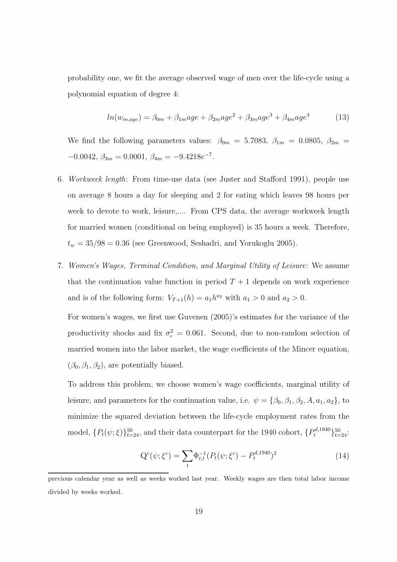
probability one, we fit the average observed wage of men over the life-cycle using a

polynomial equation of degree 4:

ln(wm,age) = β0m + β1mage+ β2mage2 + β3mage

3 + β4mage4 (13)

We find the following parameters values: β0m = 5.7083, β1m = 0.0805, β2m =

−0.0042, β3m = 0.0001, β4m = −9.4218e−7.

6. Workweek length: From time-use data (see Juster and Stafford 1991), people use

on average 8 hours a day for sleeping and 2 for eating which leaves 98 hours per

week to devote to work, leisure,.... From CPS data, the average workweek length

for married women (conditional on being employed) is 35 hours a week. Therefore,

tw = 35/98 = 0.36 (see Greenwood, Seshadri, and Yorukoglu 2005).

7. Women’s Wages, Terminal Condition, and Marginal Utility of Leisure: We assume

that the continuation value function in period T + 1 depends on work experience

and is of the following form: VT+1(h) = a1ha2 with a1 > 0 and a2 > 0.

For women’s wages, we first use Guvenen (2005)’s estimates for the variance of the

productivity shocks and fix σ2ǫ = 0.061. Second, due to non-random selection of

married women into the labor market, the wage coefficients of the Mincer equation,

(β0, β1, β2), are potentially biased.

To address this problem, we choose women’s wage coefficients, marginal utility of

leisure, and parameters for the continuation value, i.e. ψ = {β0, β1, β2, A, a1, a2}, to

minimize the squared deviation between the life-cycle employment rates from the

model, {Pt(ψ; ξ)}50t=24, and their data counterpart for the 1940 cohort, {P d,1940

t }50t=24:

Qc(ψ; ξc) =∑

t

Φ−1t,t (Pt(ψ; ξc) − P d,1940

t )2 (14)

previous calendar year as well as weeks worked last year. Weekly wages are then total labor income

divided by weeks worked.

19

where the elements of the weighting matrix, Φ−1, are equal to the variance of partici-

pation rates over the life-cycle on the diagonal and zero otherwise. The vector of cal-

ibrated parameters, ξc, is equal to: ξc = {{ϕ1940f }, {ϕ1940

a|f }, σc, σl, g1, g2, t1, t2, ρ, η, δ,

{βmi }, tw, σǫ}.19

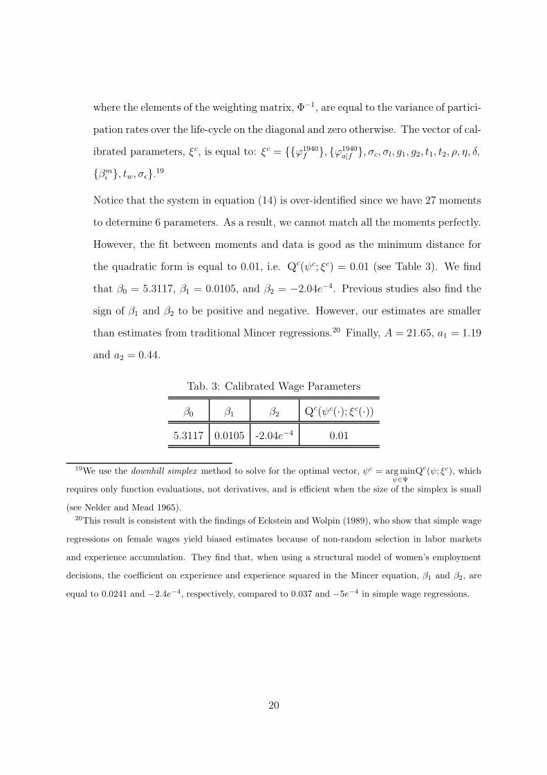
Notice that the system in equation (14) is over-identified since we have 27 moments

to determine 6 parameters. As a result, we cannot match all the moments perfectly.

However, the fit between moments and data is good as the minimum distance for

the quadratic form is equal to 0.01, i.e. Qc(ψc; ξc) = 0.01 (see Table 3). We find

that β0 = 5.3117, β1 = 0.0105, and β2 = −2.04e−4. Previous studies also find the

sign of β1 and β2 to be positive and negative. However, our estimates are smaller

than estimates from traditional Mincer regressions.20 Finally, A = 21.65, a1 = 1.19

and a2 = 0.44.

Tab. 3: Calibrated Wage Parameters

β0 β1 β2 Qc(ψc(·); ξc(·))

5.3117 0.0105 -2.04e−4 0.01

19We use the downhill simplex method to solve for the optimal vector, ψc = argminψ∈Ψ

Qc(ψ; ξc), which

requires only function evaluations, not derivatives, and is efficient when the size of the simplex is small

(see Nelder and Mead 1965).20This result is consistent with the findings of Eckstein and Wolpin (1989), who show that simple wage

regressions on female wages yield biased estimates because of non-random selection in labor markets

and experience accumulation. They find that, when using a structural model of women’s employment

decisions, the coefficient on experience and experience squared in the Mincer equation, β1 and β2, are

equal to 0.0241 and −2.4e−4, respectively, compared to 0.037 and −5e−4 in simple wage regressions.

20

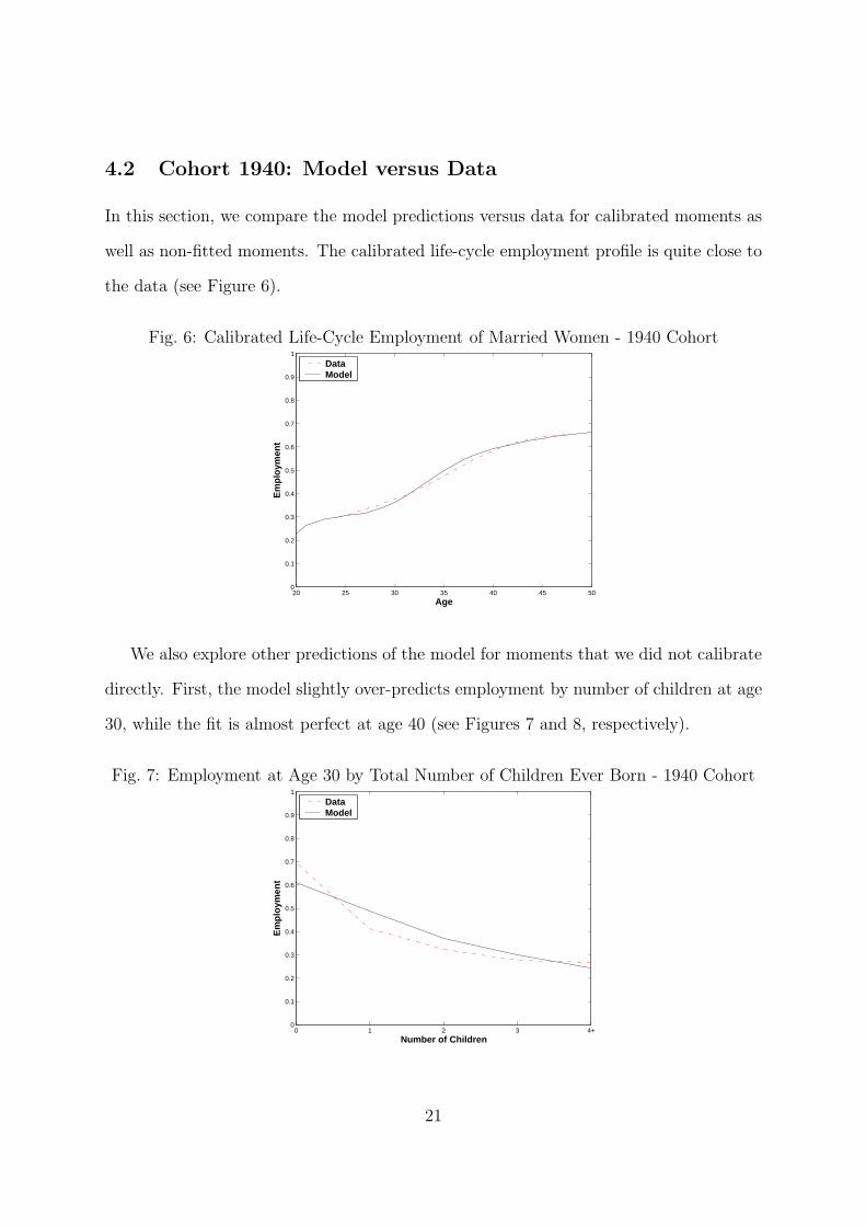
4.2 Cohort 1940: Model versus Data

In this section, we compare the model predictions versus data for calibrated moments as

well as non-fitted moments. The calibrated life-cycle employment profile is quite close to

the data (see Figure 6).

Fig. 6: Calibrated Life-Cycle Employment of Married Women - 1940 Cohort

20 25 30 35 40 45 500

0.1

0.2

0.3

0.4

0.5

0.6

0.7

0.8

0.9

1

Age

Em

ploy

men

t

DataModel

We also explore other predictions of the model for moments that we did not calibrate

directly. First, the model slightly over-predicts employment by number of children at age

30, while the fit is almost perfect at age 40 (see Figures 7 and 8, respectively).

Fig. 7: Employment at Age 30 by Total Number of Children Ever Born - 1940 Cohort

0 1 2 3 4+0

0.1

0.2

0.3

0.4

0.5

0.6

0.7

0.8

0.9

1

Number of Children

Em

ploy

men

t

DataModel

21

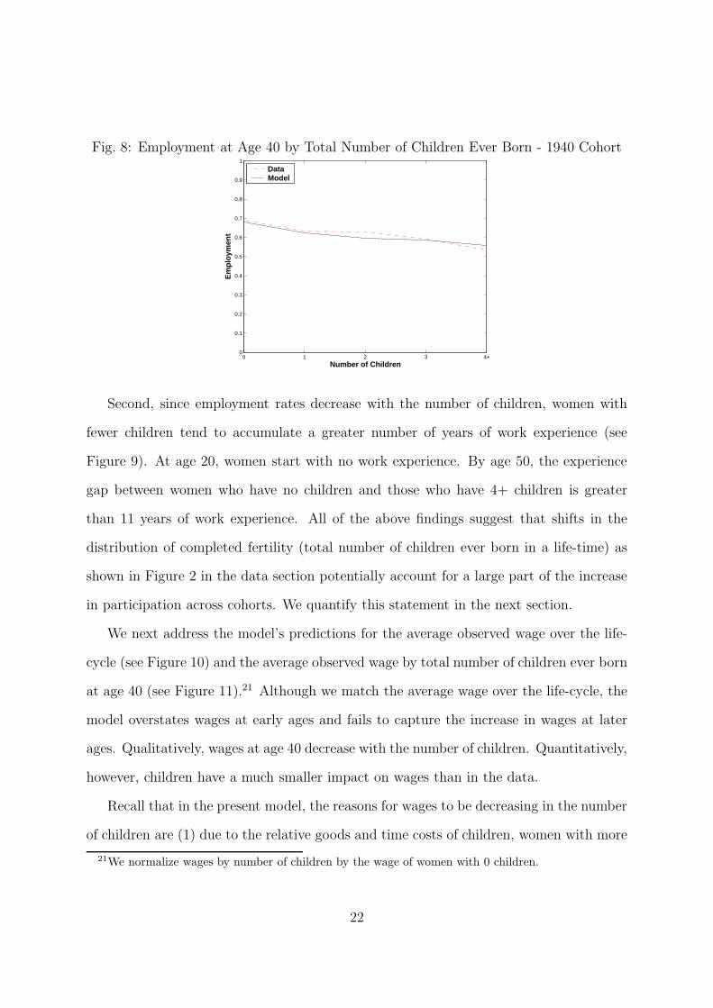
Fig. 8: Employment at Age 40 by Total Number of Children Ever Born - 1940 Cohort

0 1 2 3 4+0

0.1

0.2

0.3

0.4

0.5

0.6

0.7

0.8

0.9

1

Number of Children

Em

ploy

men

t

DataModel

Second, since employment rates decrease with the number of children, women with

fewer children tend to accumulate a greater number of years of work experience (see

Figure 9). At age 20, women start with no work experience. By age 50, the experience

gap between women who have no children and those who have 4+ children is greater

than 11 years of work experience. All of the above findings suggest that shifts in the

distribution of completed fertility (total number of children ever born in a life-time) as

shown in Figure 2 in the data section potentially account for a large part of the increase

in participation across cohorts. We quantify this statement in the next section.

We next address the model’s predictions for the average observed wage over the life-

cycle (see Figure 10) and the average observed wage by total number of children ever born

at age 40 (see Figure 11).21 Although we match the average wage over the life-cycle, the

model overstates wages at early ages and fails to capture the increase in wages at later

ages. Qualitatively, wages at age 40 decrease with the number of children. Quantitatively,

however, children have a much smaller impact on wages than in the data.

Recall that in the present model, the reasons for wages to be decreasing in the number

of children are (1) due to the relative goods and time costs of children, women with more

21We normalize wages by number of children by the wage of women with 0 children.

22

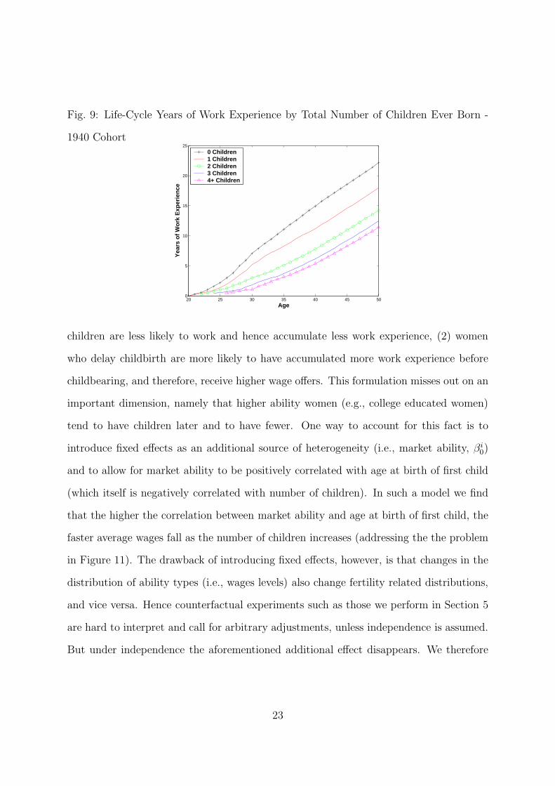
Fig. 9: Life-Cycle Years of Work Experience by Total Number of Children Ever Born -

1940 Cohort

20 25 30 35 40 45 500

5

10

15

20

25

Age

Yea

rs o

f Wor

k E

xper

ienc

e

0 Children1 Children2 Children3 Children4+ Children

children are less likely to work and hence accumulate less work experience, (2) women

who delay childbirth are more likely to have accumulated more work experience before

childbearing, and therefore, receive higher wage offers. This formulation misses out on an

important dimension, namely that higher ability women (e.g., college educated women)

tend to have children later and to have fewer. One way to account for this fact is to

introduce fixed effects as an additional source of heterogeneity (i.e., market ability, βi0)

and to allow for market ability to be positively correlated with age at birth of first child

(which itself is negatively correlated with number of children). In such a model we find

that the higher the correlation between market ability and age at birth of first child, the

faster average wages fall as the number of children increases (addressing the the problem

in Figure 11). The drawback of introducing fixed effects, however, is that changes in the

distribution of ability types (i.e., wages levels) also change fertility related distributions,

and vice versa. Hence counterfactual experiments such as those we perform in Section 5

are hard to interpret and call for arbitrary adjustments, unless independence is assumed.

But under independence the aforementioned additional effect disappears. We therefore

23

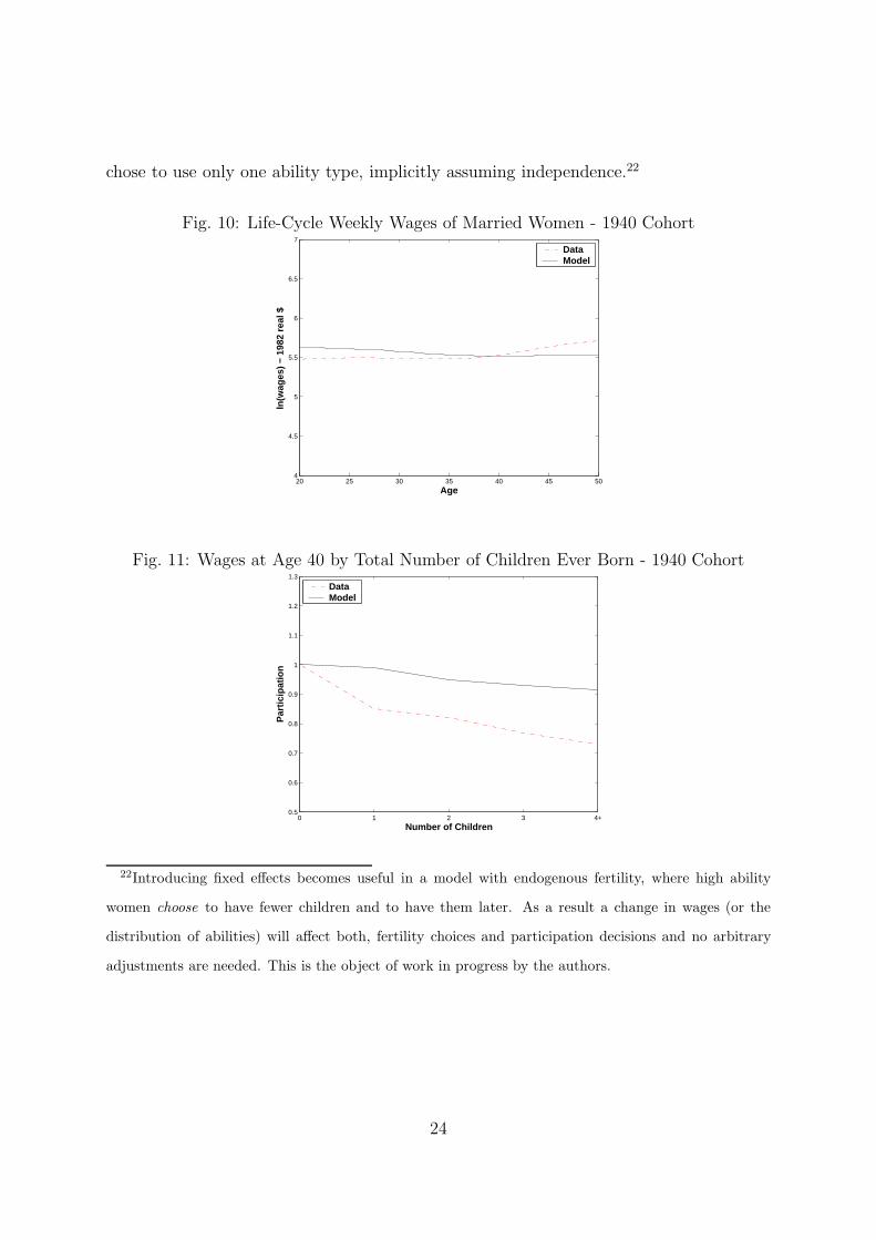
chose to use only one ability type, implicitly assuming independence.22

Fig. 10: Life-Cycle Weekly Wages of Married Women - 1940 Cohort

20 25 30 35 40 45 504

4.5

5

5.5

6

6.5

7

Age

ln(w

ages

) −

1982

rea

l $

DataModel

Fig. 11: Wages at Age 40 by Total Number of Children Ever Born - 1940 Cohort

0 1 2 3 4+0.5

0.6

0.7

0.8

0.9

1

1.1

1.2

1.3

Number of Children

Par

ticip

atio

n

DataModel

22Introducing fixed effects becomes useful in a model with endogenous fertility, where high ability

women choose to have fewer children and to have them later. As a result a change in wages (or the

distribution of abilities) will affect both, fertility choices and participation decisions and no arbitrary

adjustments are needed. This is the object of work in progress by the authors.

24

4.3 Sensitivity Analysis

In this section, we perform sensitivity analysis to assess the robustness of our calibrated

parameters. We analyze the impact of a 10-percent change in our calibrated parameters

on the goodness of fit for life-cycle participation and participation by number of children

at age 30 and 40. Changing only 1 parameter at a time, we choose women’s wages

coefficients, the marginal utility of leisure, and parameters for the continuation value to

minimize the squared deviation between the life-cycle employment rates from the model

and their data counterpart. For example, to assess the impact of a 10-percent increase

in the base goods cost, g1, we set the vector, ψ = {β0, β1, β2, A, a1, a2}, to minimize the

following quadratic form:

Qs(ψ; ξs(g1)) =∑

t

Φ−1t,t (Pt(ψ; ξs(g1)) − P d,1940

t )2 (15)

where ξs(g1) = {{ϕ1940f }, {ϕ1940

a|f }, σc, σl, 1.1g1, g2, t1, t2, ρ, η, δ, {βmi }, tw, σǫ}. Let ψs(g1) =

arg minψ∈Ψ

Qs(ψ; ξs(g1)), the solution to the above system. We calculate the percentage

change (elasticity) in the coefficients of women’s wages and marginal utility of leisure as

follows: λψi,g1 =ψs

i(g1)−ψc

i

ψc

i

/∆g1g1

. We assess the impact of a 10-percent change in parameters

for preferences, cost of children, and the standard deviation of the productivity shock and

present our results in Table 4.

Since the marginal utility of consumption for women with children is very high, the re-

lationship between employment and number of children flattens out following an increase

in the base goods cost of children, g1 (relative to g2).23 The decrease in employment rates

of women with 0 and 1 child is achieved through an increase in the marginal utility of

leisure, A, and a decrease in returns to work experience, (β1, β2). On the other hand,

when the base time cost t1 is high relative to t2, the marginal utility of leisure for women

with children is very high. As a result, the relationship between employment and number

23For very high values of g1 relative to g2, the marginal utility of consumption for women with children

is so high that employment rates increases with the number of children, which is counterfactual.

25

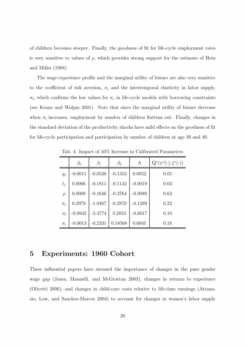
of children becomes steeper. Finally, the goodness of fit for life-cycle employment rates

is very sensitive to values of ρ, which provides strong support for the estimate of Hotz

and Miller (1988).

The wage-experience profile and the marginal utility of leisure are also very sensitive

to the coefficient of risk aversion, σc and the intertemporal elasticity in labor supply,

σl, which confirms the low values for σc in life-cycle models with borrowing constraints

(see Keane and Wolpin 2001). Note that since the marginal utility of leisure decrease

when σl increases, employment by number of children flattens out. Finally, changes in

the standard deviation of the productivity shocks have mild effects on the goodness of fit

for life-cycle participation and participation by number of children at age 30 and 40.

Tab. 4: Impact of 10% Increase in Calibrated Parameters

β0 β1 β2 A Qs(ψs(·); ξs(·))

g1 -0.0011 -0.0538 -0.1353 0.0052 0.05

t1 0.0006 -0.1811 -0.1142 -0.0019 0.03

ρ 0.0008 -0.1646 -0.3764 -0.0080 0.63

σc 0.2979 -1.0467 -0.2870 -0.1289 0.22

σl -0.0942 -3.4774 3.2853 -0.6017 0.10

σǫ -0.0013 -0.2331 0.18568 0.0045 0.18

5 Experiments: 1960 Cohort

Three influential papers have stressed the importance of changes in the pure gender

wage gap (Jones, Manuelli, and McGrattan 2003), changes in returns to experience

(Olivetti 2006), and changes in child-care costs relative to life-time earnings (Attana-

sio, Low, and Sanchez-Marcos 2004) to account for changes in women’s labor supply

26

either over time or across cohorts. In this section, we assess the quantitative importance

of these 3 forces as follows.

Taking changes in fertility patterns into account, we use our model to quantify what

changes in women’s wages and child-care cost are needed to match the life-cycle par-

ticipation choices of women born in 1960. Using distributions for number and timing

of births of the 1960 cohort, we choose the pure gender wage gap, β0 (relative to β0m),

the returns to experience, β1, β2, and the cost of child-care, g2, to match the life-cycle

employment rates of the 1960 cohort, holding all other calibrated parameters constant.

We set the vector, ψ = {β0, β1, β2, g2}, to minimize the following quadratic form:

Qe(ψ; ξe) =∑

t

Φ−1t,t (Pt(ψ; ξe) − P d,1960

t )2 (16)

where ξe = {{ϕ1960f }, {ϕ1960

a|f }, σc, σl, A, g1, t1, t2, ρ, η, δ, {βmi }, tw, σǫ, a1, a2}.

Let ψe = arg minψ∈Ψ

Qe(ψ; ξe), the solution to the above system. This exercise allows us to

answer questions such as: taking into account changes in fertility patterns, by how much

do the coefficients of women’s Mincer wage equation and child-care cost need to change

to explain the observed patterns in women’s employment?

Our model has the same qualitative predictions as in Jones, Manuelli, and McGrat-

tan (2003), Olivetti (2006), or Attanasio, Low, and Sanchez-Marcos (2004). The pure

gender wage gap and the child-care cost decrease, while returns to experience increase

across cohorts in order to match changes in women’s employment across cohorts (see

Table 5). Quantitatively, however, we find that these changes are smaller than previously

reported in these papers. The pure gender wage gap decreases, i.e. β0 increases by less

than 1 percent, returns to experience increase as the coefficient on experience, β1, and

experience squared, β2, increase by 43 percent and 21 percent, respectively, and finally

the price of child-care, g2, decreases by 18 percent.

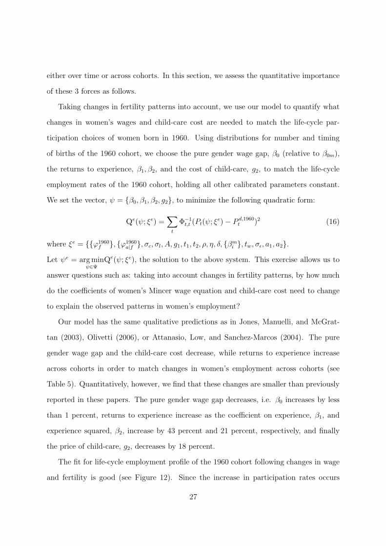
The fit for life-cycle employment profile of the 1960 cohort following changes in wage

and fertility is good (see Figure 12). Since the increase in participation rates occurs

27

mainly for women with 1 and 2 children, the experience gap between women with 0 and

1 child is less than 1.5 year at age 43 compared to more than 5 years for women born in

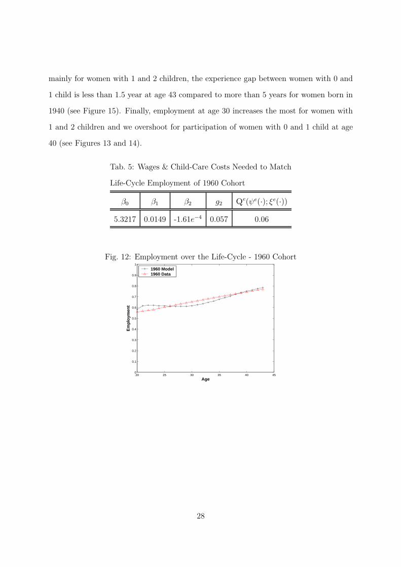
1940 (see Figure 15). Finally, employment at age 30 increases the most for women with

1 and 2 children and we overshoot for participation of women with 0 and 1 child at age

40 (see Figures 13 and 14).

Tab. 5: Wages & Child-Care Costs Needed to Match

Life-Cycle Employment of 1960 Cohort

β0 β1 β2 g2 Qe(ψe(·); ξe(·))

5.3217 0.0149 -1.61e−4 0.057 0.06

Fig. 12: Employment over the Life-Cycle - 1960 Cohort

20 25 30 35 40 450

0.1

0.2

0.3

0.4

0.5

0.6

0.7

0.8

0.9

1

Age

Em

ploy

men

t

1960 Model1960 Data

28

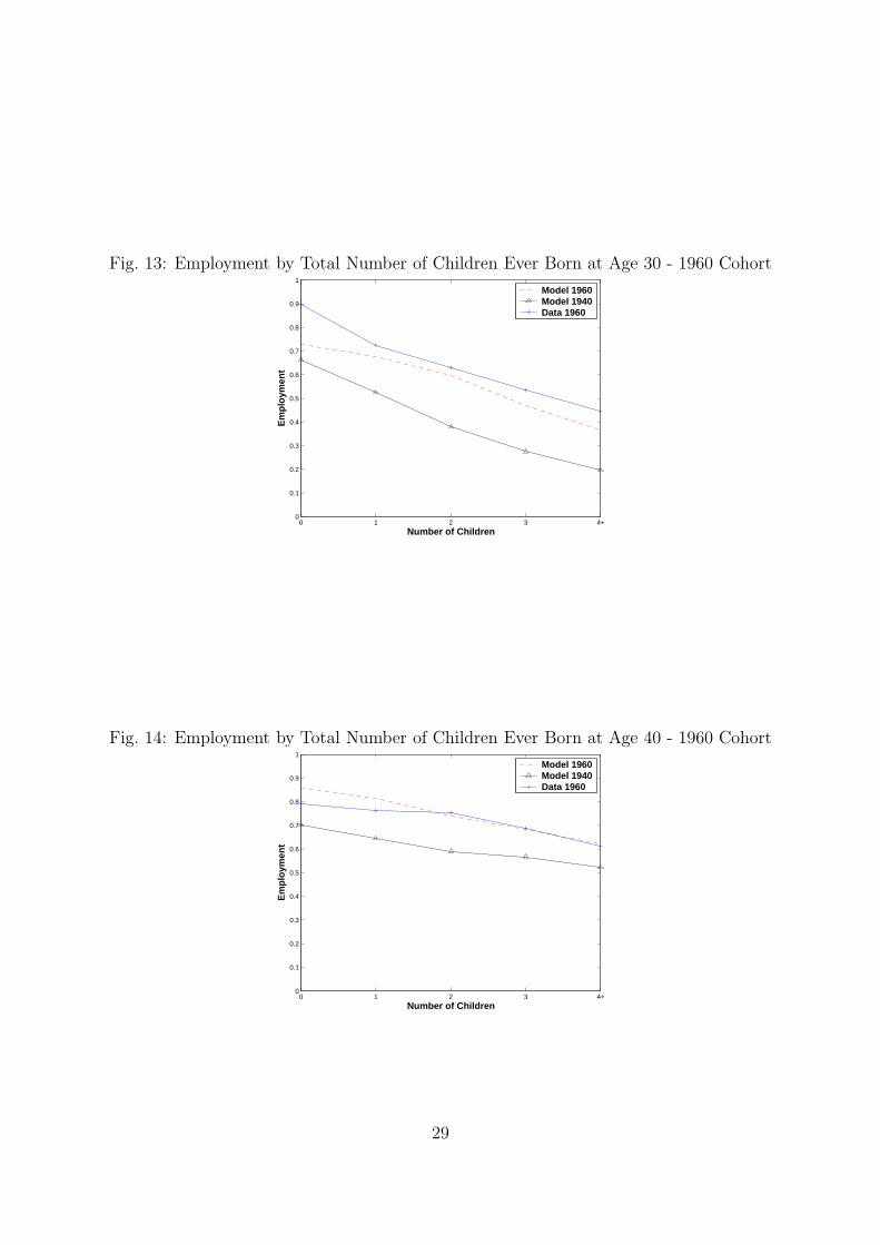
Fig. 13: Employment by Total Number of Children Ever Born at Age 30 - 1960 Cohort

0 1 2 3 4+0

0.1

0.2

0.3

0.4

0.5

0.6

0.7

0.8

0.9

1

Number of Children

Em

ploy

men

tModel 1960Model 1940Data 1960

Fig. 14: Employment by Total Number of Children Ever Born at Age 40 - 1960 Cohort

0 1 2 3 4+0

0.1

0.2

0.3

0.4

0.5

0.6

0.7

0.8

0.9

1

Number of Children

Em

ploy

men

t

Model 1960Model 1940Data 1960

29

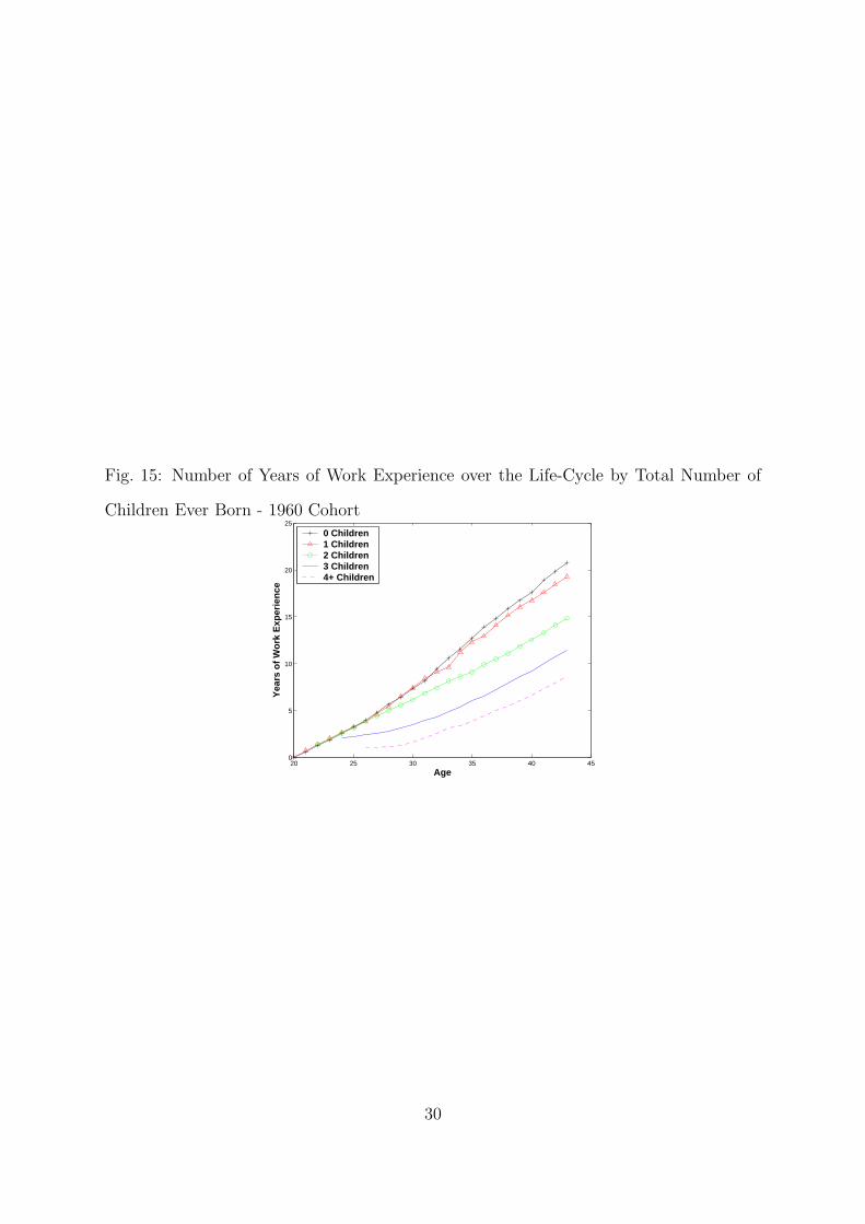
Fig. 15: Number of Years of Work Experience over the Life-Cycle by Total Number of

Children Ever Born - 1960 Cohort

20 25 30 35 40 450

5

10

15

20

25

Age

Yea

rs o

f Wor

k E

xper

ienc

e

0 Children1 Children2 Children3 Children4+ Children

30

Since we implicitly assumed that changes in fertility patterns, gender wage differen-

tials, and cost of child-care account for 100-percent of changes in women’s employment

across cohorts, we perform a decomposition exercise to assess their relative (quantitative)

importance. We write:

1 = ∆(Fertility) + ∆(Wages) + ∆(Child-Care) +R (17)

where changes in fertility include changes in number and timing of births, changes in

wages include changes in the pure gender wage gap and returns to experience, and R is a

residual term to account for potential interaction between all the variables. We present

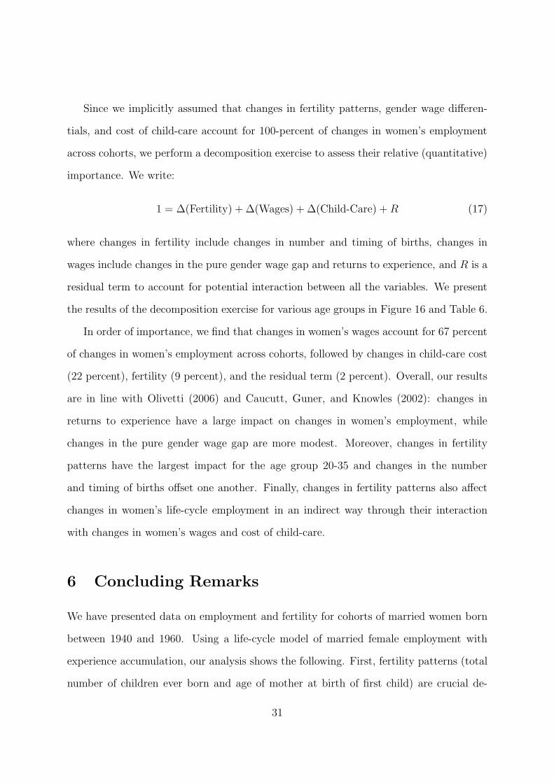
the results of the decomposition exercise for various age groups in Figure 16 and Table 6.

In order of importance, we find that changes in women’s wages account for 67 percent

of changes in women’s employment across cohorts, followed by changes in child-care cost

(22 percent), fertility (9 percent), and the residual term (2 percent). Overall, our results

are in line with Olivetti (2006) and Caucutt, Guner, and Knowles (2002): changes in

returns to experience have a large impact on changes in women’s employment, while

changes in the pure gender wage gap are more modest. Moreover, changes in fertility

patterns have the largest impact for the age group 20-35 and changes in the number

and timing of births offset one another. Finally, changes in fertility patterns also affect

changes in women’s life-cycle employment in an indirect way through their interaction

with changes in women’s wages and cost of child-care.

6 Concluding Remarks

We have presented data on employment and fertility for cohorts of married women born

between 1940 and 1960. Using a life-cycle model of married female employment with

experience accumulation, our analysis shows the following. First, fertility patterns (total

number of children ever born and age of mother at birth of first child) are crucial de-

31

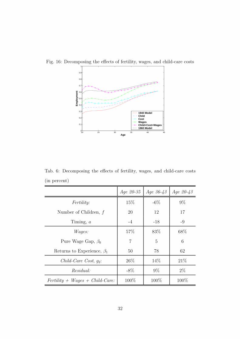
Fig. 16: Decomposing the effects of fertility, wages, and child-care costs

20 25 30 35 40 450

0.1

0.2

0.3

0.4

0.5

0.6

0.7

0.8

0.9

1

Age

Em

ploy

men

t

1940 ModelChildCostWagesChild+Cost+Wages1960 Model

Tab. 6: Decomposing the effects of fertility, wages, and child-care costs

(in percent)

Age 20-35 Age 36-43 Age 20-43

Fertility: 15% -6% 9%

Number of Children, f 20 12 17

Timing, a -4 -18 -9

Wages: 57% 83% 68%

Pure Wage Gap, β0 7 5 6

Returns to Experience, β1 50 78 62

Child-Care Cost, g2: 26% 14% 21%

Residual: -8% 9% 2%

Fertility + Wages + Child-Care: 100% 100% 100%

32

terminants of the life-cycle employment profile for married women. Second, changes in

gender wage differentials and costs of children needed to account for changes in women’s

life-cycle employment are smaller than previously found in the literature once we take

into account changes in fertility patterns. Third, changes in women’s wages (in particular,

returns to experience) have the largest impact on women’s employment decisions.

One open question is: What caused the decrease and delay in fertility? Our current

work in progress is to endogenize fertility and timing of births decisions to ask whether

changes in wages can also account for the delay in fertility. Preliminary results show

that the delay, though positive, is largely left unaccounted for. Something else seems

to have caused the delay in fertility. Several related questions come to mind: How is

fertility related to the marriage decision? Was the change in fertility decisions simply

due to cultural changes and changes in social norms? In what sense and can we attempt

to measure these changes? The answers to these questions are closely intermingled and

hard to disentangle from the question about why women tend to have children later and

take care of them differently than they used to. They are however crucial to set up

a useful model of fertility choices in terms of number and timing of births as well as

child-care arrangements.

The other open question is why wage levels and returns to experience changed more

for women than they did for men. Besides straight out discrimination, many other more

readily quantifiable hypotheses can be considered. Changing occupational opportunities

due to the rise in the service sector, changing educational investments pertaining more

to women than men because of initial conditions are only a few avenues to be explored

further.

33

7 Appendix

7.1 Life-cycle Patterns by Education

We present data for life-cycle employment profiles and fertility by education.

7.1.1 Employment

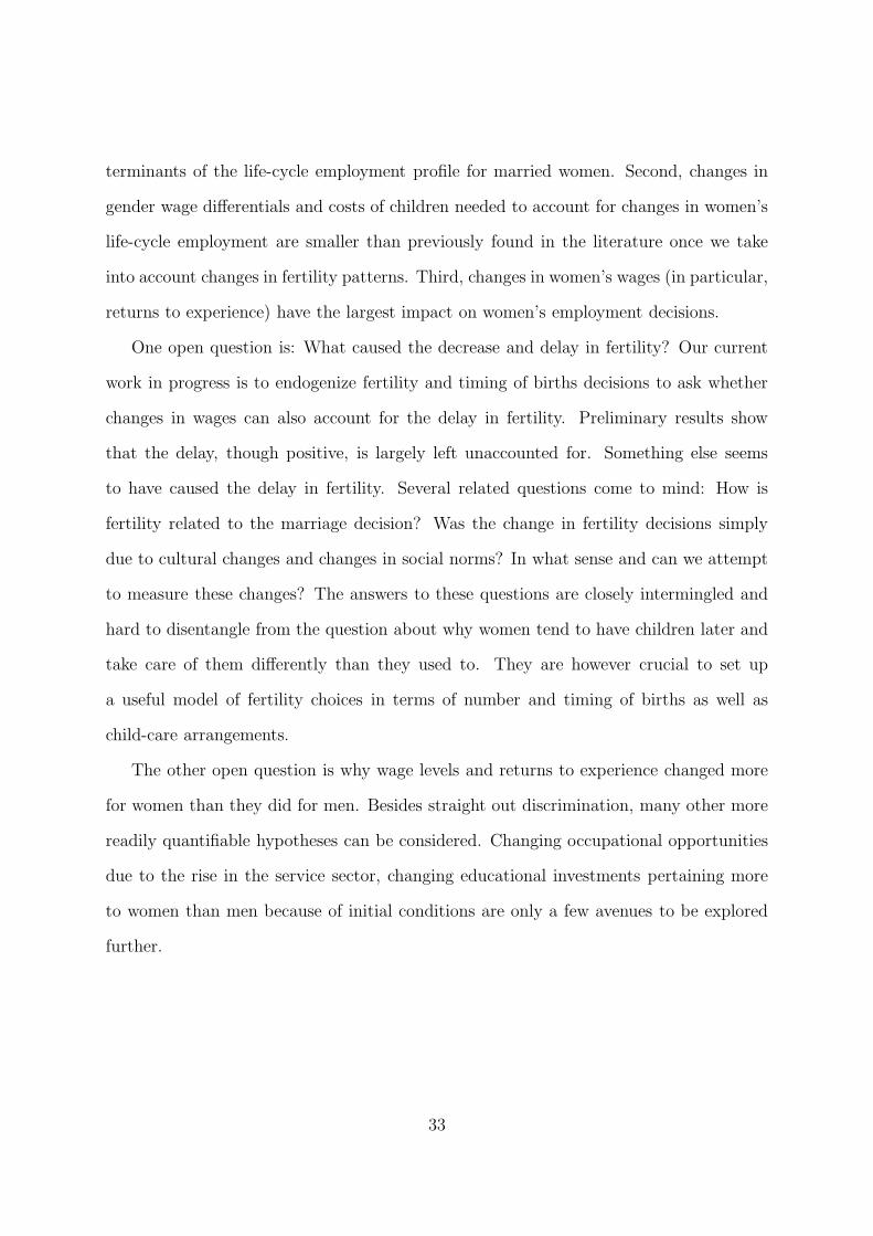
Employment profiles over the life-cycle and their changes across cohorts differ consider-

ably by education. They are mostly increasing in age for high school graduates, while

college women tend to work a lot before childbearing ages, then drop out of the labor

force and finally join the labor force again after childbearing ages (see Figures 17 and 18,

respectively).

Fig. 17: Life-Cycle Employment Profile of Married Women by Cohort - High School

Graduates

20 25 30 35 40 45 500

0.1

0.2

0.3

0.4

0.5

0.6

0.7

0.8

0.9

1

Age

Par

ticip

atio

n

Born in 19401960

However, changes in employment rates across cohorts are the largest at childbearing

ages. Between age 20 and 35, employment rates increased on average by 26 and 27

percentage points for high school and college graduates respectively. Between age 36

and 50, employment only increases by 10 and 4 percentage points for HS and College

graduates.

34

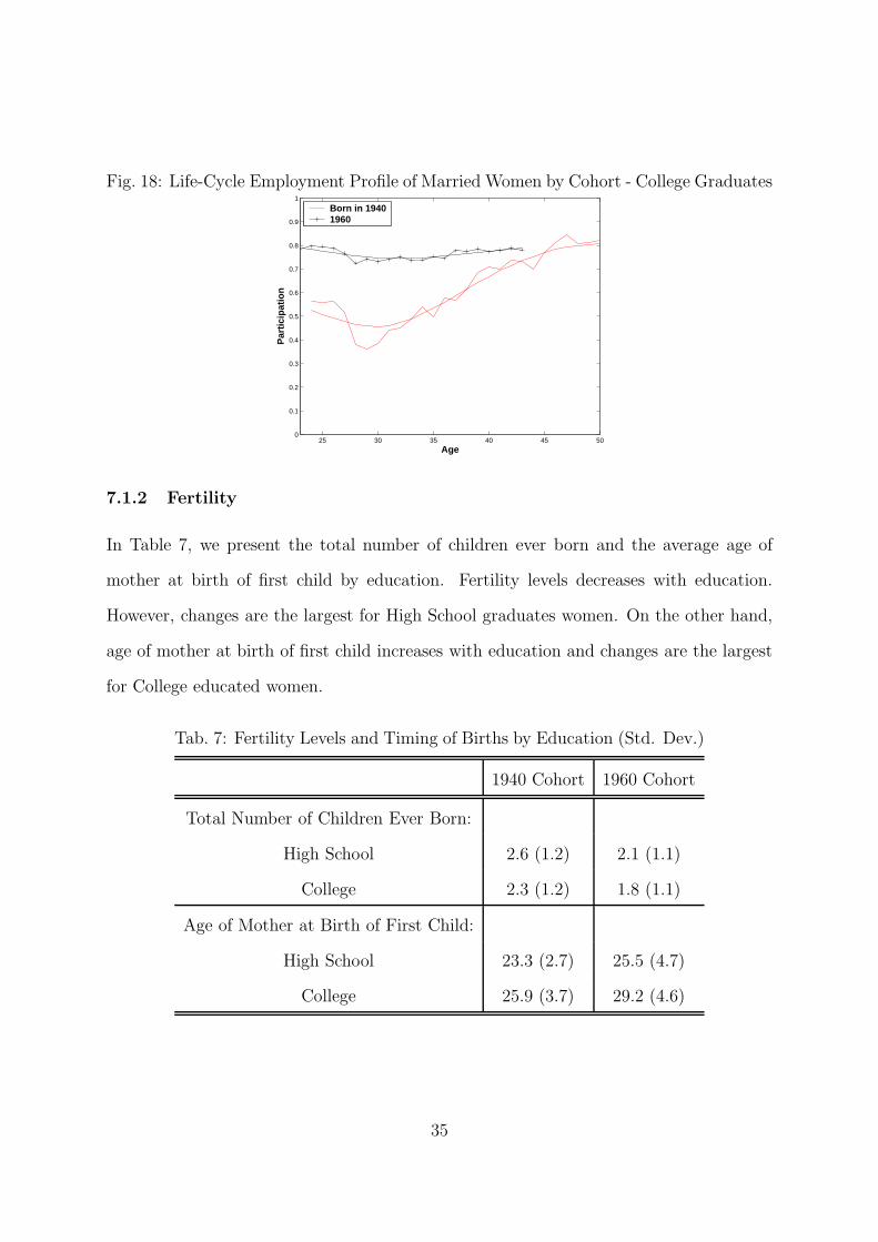
Fig. 18: Life-Cycle Employment Profile of Married Women by Cohort - College Graduates

25 30 35 40 45 500

0.1

0.2

0.3

0.4

0.5

0.6

0.7

0.8

0.9

1

Age

Par

ticip

atio

n

Born in 19401960

7.1.2 Fertility

In Table 7, we present the total number of children ever born and the average age of

mother at birth of first child by education. Fertility levels decreases with education.

However, changes are the largest for High School graduates women. On the other hand,

age of mother at birth of first child increases with education and changes are the largest

for College educated women.

Tab. 7: Fertility Levels and Timing of Births by Education (Std. Dev.)

1940 Cohort 1960 Cohort

Total Number of Children Ever Born:

High School 2.6 (1.2) 2.1 (1.1)

College 2.3 (1.2) 1.8 (1.1)

Age of Mother at Birth of First Child:

High School 23.3 (2.7) 25.5 (4.7)

College 25.9 (3.7) 29.2 (4.6)

35

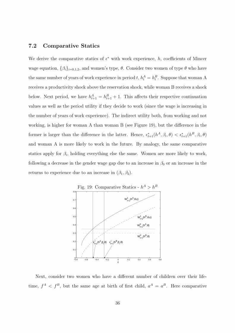
7.2 Comparative Statics

We derive the comparative statics of ǫ∗ with work experience, h, coefficients of Mincer

wage equation, {βi}i=0,1,2, and women’s type, θ. Consider two women of type θ who have

the same number of years of work experience in period t, hAt = hBt . Suppose that woman A

receives a productivity shock above the reservation shock, while woman B receives a shock

below. Next period, we have hAt+1 = hBt+1 + 1. This affects their respective continuation

values as well as the period utility if they decide to work (since the wage is increasing in

the number of years of work experience). The indirect utility both, from working and not

working, is higher for woman A than woman B (see Figure 19), but the difference in the

former is larger than the difference in the latter. Hence, ǫ∗t+1(hA, βi, θ) < ǫ∗t+1(h

B, βi, θ)

and woman A is more likely to work in the future. By analogy, the same comparative

statics apply for βi, holding everything else the same. Women are more likely to work,

following a decrease in the gender wage gap due to an increase in β0 or an increase in the

returns to experience due to an increase in (β1, β2).

Fig. 19: Comparative Statics - hA > hB

−0.8 −0.6 −0.4 −0.2 0 0.2 0.4 0.6 0.80

0.1

0.2

0.3

0.4

0.5

0.6

0.7

0.8

ε

εt+1∗ (hB,β

i,θ) ε

t+1∗ (hA,β

i,θ)

W0t+1

(hA,θ)

W0t+1

(hB,θ)

W1t+1

(hA,θ,ε)

W1t+1

(hB,θ,ε)

Next, consider two women who have a different number of children over their life-

time, fA < fB, but the same age at birth of first child, aA = aB. Here comparative

36

statics depend on the relative magnitudes of time and goods costs. For sake of intuition,

consider two extreme cases. In the first case, children are costly if the woman works,

while in the second, they are costly if she doesn’t work. Therefore, in case (1) (case (2)),

women with fewer children are more (less) likely to work. In the data section above,

we described employment by number of children in the household and found that it is

decreasing. Calibrating to this fact, parameters adjust such that a version of case (1)

applies. Therefore, under our parameters, the reservation shock is higher for women

who have more children over their life-time. Thus, they are less likely to work. Finally,

consider two women who differ in their age at birth of first child, i.e. aA > aB, but will

have the same number of children over their life-time, fA = fB. Then for some periods,

woman A will have fewer children than woman B. She will therefore be more likely to

work, everything else the same. However, once she starts to have children herself, she

will have younger children in the household than woman B. Since younger children are

costlier, she is less likely to work during those periods.

37

References

[1] Joseph G. Altonji. Intertemporal substitution in labor supply: Evidence from micro

data. Journal of Political Economy, 94(3):S176–S215, June 1986.

[2] Sumru Altug and Robert A. Miller. The effect of work experience on female wages

and labor supply. Review of Economic Studies, 65(1):45–85, January 1998.

[3] Orazio Attanasio, Hamish Low, and Virginia Sanchez-Marcos. Explaining changes

in female labour supply in a life-cycle model. Working Paper, University College

London, March 2004.

[4] Raquel Bernal. The effect of maternal employment and child care on children’s

cognitive development. Working Paper, Northwestern University, 2004.

[5] Elizabeth M. Caucutt, Nezih Guner, and John Knowles. Why do women wait?

matching, wage inequality, and the incentives for fertility delay. The Review of

Economic Dynamics, 5(4):815–855, oct 2002.

[6] Zvi Eckstein and Gerard J. van der Berg. Empirical labor search: A survey. Journal

of Econometrics, forthcoming, 2006.

[7] Zvi Eckstein and Kenneth I. Wolpin. Dynamic labour force participation of mar-

ried women and endogenous work experience. The Review of Economic Studies,

56(3):375–390, July 1989.

[8] Andres Erosa, Luisa Fuster, and Diego Restuccia. A quantitative theory of the

gender wage gap in wages. Working Paper, University of Toronto, 2005.

[9] Thomas J. Espenshade. Investing in Children: New Estimates of Parental Expendi-

tures. Washington, D.C.: Urban Institute Press, 1984.

38

[10] Raquel Fernandez, Alessandra Fogli, and Claudia Olivetti. Preference formation

and the rise of women’s labor force participation: Evidence from WWII. NBER

Working Paper 10589, National Bureau of Economic Research, 2004.

[11] Marco Francesconi. A joint dynamic model of fertility and work of married women.

Journal of Labor Economics, 20(2):336–380, 2002.

[12] Oded Galor and David N. Weil. The gender gap, fertility and growth. American

Economic Review, 86(3):374–87, June 1996.

[13] Claudia Goldin and Lawrence F. Katz. The power of the pill: Oral contraceptives and

women’s career and marriage decisions. Journal of Political Economy, 110(4):730–

770, August 2002.

[14] Jeremy Greenwood, Ananth Seshadri, and Mehmet Yorukoglu. Engines of liberation.

The Review of Economic Studies, 72(1):109–133, January 2005.

[15] Fatih Guvenen. Learning your income: Are labor income shocks really very persis-

tent? Working Paper, University of Rochester, 2005.

[16] Gary D. Hansen. Indivisible labor and the business cycle. Journal of Monetary

Economics, 16:309–27, November 1985.

[17] Lars Peter Hansen and James J. Heckman. The empirical foundations of calibration.

Journal of Economic Perspectives, 10(1):87–104, Winter 1996.

[18] James J. Heckman, Lance J. Lochner, and Petra E. Todd. Fifty years of mincer

earnings regressions. Working Paper 9732, National Bureau of Economic Research,

2003.

[19] James J. Heckman and James R. Walker. The relationship between wages and

39

income and the timing and spacing of births: Evidence from swedish longitudinal

data. Econometrica, 58(6):1411–1441, November 1990.

[20] Russell C. Hill and Frank P. Stafford. Parental care of children: Time diaries

estimates of quantity, predictability, and variety. Journal of Human Resources,

15(2):220–239, Spring 1980.

[21] Joseph V. Hotz and Robert A. Miller. An empirical analysis of life cycle fertility and

female labor supply. Econometrica, 56(1):91–118, January 1988.

[22] Glenn R. Hubbard, Jonathan Skinner, and Stephen P. Zeldes. The importance

of precautionary motives in explaining individual and aggregate saving. Carnegie-

Rochester Conference Series on Public Policy, 40:59–125, June 1994.

[23] Susumu Imai and Michael P. Keane. Intertemporal labor supply and human capital

accumulation. International Economic Review, 45(2):601–641, May 2004.

[24] Larry E. Jones, Rodolfo Manuelli, and Ellen S. McGrattan. Why are married women

working so much? Federal Reserve Bank of Minneapolis Staff Report, May 2003.

[25] Thomas F. Juster and Frank P. Stafford. The allocation of time: Empirical findings,

behavioral models, and problems of measurement. Journal of Economic Literature,

29(2):471–522, June 1991.

[26] Michael P. Keane and Kenneth I. Wolpin. The effect of parental transfers and

borrowing constraints on educational attainment. International Economic Review,

42(4):1051–1103, November 2001.

[27] Miles S. Kimball. Precautionary saving in the small and in the large. Econometrica,

58(1):53–73, January 1990.

40

[28] Finn E. Kydland. Cycles and aggregate labor market fluctuations. In Thomas F.

Cooley, editor, Frontiers of Business Cycle Research, chapter 5, pages 126–156.

Princeton University Press, Princeton, NJ, 1995.

[29] Finn E. Kydland and Edward C. Prescott. Time to build and aggregate fluctuations.

Econometrica, 50(6):1345–1370, November 1982.

[30] Edward P. Lazear and Robert T. Michael. Family size and the distribution of real

per capita income. American Economic Review, 70(1):91–107, March 1980.

[31] Thomas E. MaCurdi. An empirical model of labor supply in a life-cycle setting.

Journal of Political Economy, 89(6):1059–85, December 1981.

[32] Costas Meghir and Luigi Pistaferri. Income variance dynamics and heterogeneity.

Econometrica, 72(1):1–32, January 2004.

[33] John A. Nelder and Roger Mead. A simplex method for function minimization.

Computer Journal, 7:308–313, 1965.

[34] Claudia Olivetti. Changes in women’s hours of work: The effect of changing returns

to experience. Review of Economics Dynamics, forthcoming, June 2006.

[35] Edward C. Prescott. Theory ahead of business cycle measurement. Quarterly Review

Minneapolis Federal Reserve Bank, 10:9–22, Fall 1986.

[36] Alice Schoonbroodt. Small sample bias using maximum likelihood versus moments:

The case of a simple search model of the labor market. Working Paper, University

of Minnesota, September 2002.

[37] Wilbert Van der Klaauw. Female labour supply and marital status decisions: A

life-cycle model. Review of Economic Studies, 63(2):199–235, April 1996.

41